Data-driven unsteady aeroelastic modeling for control

Data-driven unsteady aeroelastic modeling for controlMichelle K. Hickner∗ and Urban Fasel†

University of Washington, Seattle, WA 98195

Aditya G. Nair‡University of Nevada, Reno, NV 89557

Bingni W. Brunton§ and Steven L. Brunton¶

University of Washington, Seattle, WA 98195

Aeroelastic structures, from insect wings to wind turbine blades, experience transient un-

steady aerodynamic loads that are coupled to their motion. Effective real-time control of

flexible structures relies on accurate and efficient predictions of both the unsteady aeroelastic

forces and airfoil deformation. For rigid wings, classical unsteady aerodynamic models have

recently been reformulated in state-space for control and extended to include viscous effects.

Here we further extend this modeling framework to include the deformation of a flexible wing

in addition to the quasi-steady, added mass, and unsteady viscous forces. We develop low-order

linear models based on data from direct numerical simulations of flow past a flexible wing at

low Reynolds number. We demonstrate the effectiveness of these models to track aggressive

maneuvers with model predictive control while constraining maximum wing deformation. This

system identification approach provides an interpretable, accurate, and low-dimensional repre-

sentation of an aeroelastic system that can aid in system and controller design for applications

where transients play an important role.

Keywords– Aeroelasticity, unsteady aerodynamics, system identification, reduced order model-

ing, Theodorsen’s model, flutter, model predictive control∗PhD Student, Department of Mechanical Engineering, Box 352600, corresponding author ([email protected])†Postdoctoral Researcher, Department of Mechanical Engineering‡Assistant Professor, Department of Mechanical Engineering§Associate Professor, Department of Biology¶Professor, Department of Mechanical Engineering

arX

iv:2

111.

1129

9v2

[ph

ysic

s.fl

u-dy

n] 1

2 Ja

n 20

22

Nomenclature𝛼 angle of attack of plate

^ curvature near leading edge of plate

a kinematic viscosity

𝜏 convective time (dimensionless), 𝜏 ≡ 𝑡𝑈∞/𝑐

Δ𝜏 time step

Δ𝜏𝑐 coarse time step, duration of impulse

𝑎 pitch axis location relative to the 1/2 chord

𝑐 chord length of plate

𝑟 model rank

𝑡 time

x state vector of state-space model

A, B, C state-space matrices identified by ERA

𝐶𝛼 angle of attack (lift slope) coefficient

𝐶 ¤𝛼, 𝐶 ¥𝛼 added mass coefficients

𝐶𝐿 coefficient of lift

𝐸𝐼 plate flexural rigidity

H Hankel matrix, time-delay matrix of measurements

𝐾𝐵 plate bending stiffness

𝑀𝜌 mass ratio

Q MPC weights for outputs

R MPC weights for inputs

𝑅𝑒 Reynolds number, 𝑅𝑒 ≡ 𝑈∞𝑐/a

RΔ𝑢 MPC weights for input rate of change

𝑇𝑐 MPC control horizon

𝑇𝑝 MPC prediction horizon

𝑈∞ free stream velocity

Y matrix of measurements

Y Markov parameters 2

I. IntroductionWing flexibility plays a major role in aerodynamic systems, both natural and engineered, by increasing efficiency

and mitigating structural damage from sudden loading [1, 2]. The effect of wing flexibility has been long studied in

the context of bio-locomotion [3–23], where it is known that flexibility has favorable aerodynamic and hydrodynamic

properties.

There is an increasing need to develop unsteady aeroelastic models to realize these benefits for engineering systems,

for example to control autonomous flight vehicles, including at sizes comparable to insects and birds. The benefits of

wing flexibility are often the consequences of subtle aeroelastic effects, and for many applications it is important to

capture unsteady viscous fluid transients. This work develops accurate and efficient models to capture these effects in

design and control efforts.

Aeroelastic modeling is challenging because of the strongly coupled fluid-structure interactions, which are difficult

to capture in reduced-order models. Existing high-fidelity models can simulate the coupled fluid flow fields and the

deformation profile of a structure [24–26], but they are computationally intensive and do not fit readily into model-based

control design. Medium fidelity models, such as doublet-lattice methods [27], strip theory [28], and panel methods [29]

are widely-used approaches that can be combined with optimization to aid in aeroelastic design [30], but they neglect

viscous effects and are not well suited for real-time control. The unsteady vortex-lattice method provides some balance

between accuracy and tractability for control; however, it has limitations for wings with significant camber or viscous

effects [31, 32]. Other nonlinear modeling approaches include Volterra kernels [33, 34] and modal models [35–37],

although there are considerably fewer control techniques for nonlinear systems [38, 39]. Moreover, linear models are

often sufficient for even large amplitude motions [40] until leading edge separation and stall [41].

Reduced-order models have been developed for the control of lift, including those with significant viscous and

unsteady effects, extending the classic inviscid Theodorsen [42] and Wagner models [43] based on viscous flow

data [40, 44–47]. These linear unsteady aerodynamic models take advantage of data-driven system identification

methods, such as the eigensystem realization algorithm (ERA) [48] and quasi-linear parameter varying techniques

(qLPV) to develop minimal realizations that are both accurate and computationally efficient enough for real-time

control. Data-driven techniques avoid the simplifying assumptions built into some analytical models, such as inviscid or

quasi-steady flow, allowing models to be used in a wider range of flow conditions, including low Reynolds number flows

and those resulting from rapid, large-amplitude maneuvers.

In this work, we extend these rigid low-order unsteady aerodynamic models to include the effect of wing flexibility

and demonstrate these models for the control of aggressive maneuvers. The resulting linear state-space models are

purely data-driven, so that they may be tailored to specific wing geometries and flow conditions. In particular, time

series data of lift and wing deformation are used to build a model without requiring information about the material

properties or mass distribution of the wing. Extending the model to predict wing deformation is key for control in

3

Fig. 1 A linear state-space model of an aeroelastic wing is developed from lift and deformation observations.The model separates the contributions from transients, quasi-steady pitch effects, and added mass. The modelis used to track reference 𝐶𝐿 and curvature, ^.

aeroelastic applications, to reduce material fatigue due to vibrations or structural failures due to large stresses. The ERA

algorithm is used to augment the limited measurement data with time delayed information, enabling a reduced-order

model for fast computation in real-time control. We demonstrate this approach on data from a high-fidelity direct

numerical simulation of a flexible wing in a low Reynolds number flow. Specifically, this model is used for model

predictive control (MPC) of an aggressive lift trajectory, while simultaneously minimizing deflection.

Figure 1 shows a schematic of the modeling framework, including the training data, the state-space model, and

control results. The model developed is in linear state-space form, allowing straightforward conversion to the frequency

domain, providing information about resonance behavior. While flutter suppression is often done by tuning mass

distribution in the design process, or more recently, with active control of the wing shape, this method shows promise

for flutter suppression through pitching motions only, without any need for actively morphing wings.

II. BackgroundHere we provide a brief overview of some of the most relevant background material on data-driven unsteady

aerodynamic modeling and control. Section II.A introduces Theodorsen’s model and describes a data-driven extension

for a rigid plate [45], which serves as the foundation for the aeroelastic modelling procedure developed in this paper.

This modelling procedure uses the eigensystem realization algorithm, which is described in section II.B. Finally, model

predictive control is introduced in section II.C because it is well suited to aeroelastic control due to its ability to constrain

deformation.

4

A. Empirical Theodorsen model: a data-driven approach

Two of the earliest and most important unsteady aerodynamic models for the lift on a flat plate in response to motion

are those developed by Wagner [43] in 1925 and Theodorsen [42] in 1935. These models, which would later be shown to

be equivalent [49, 50], describe the unsteady lift on a two-dimensional pitching and/or plunging flat plate in an inviscid,

incompressible fluid. Both models analytically represent the unsteady lift as a function of angle of attack, added mass

effects, and the vorticity of an idealized planar wake.

Theodorsen’s model for thin airfoils describes the forces and moments on an airfoil for harmonic motions.

Theodorsen’s model assumes an idealized planar wake in an inviscid, incompressible flow. For pure pitching motion

with dimensional frequency 𝑓 , the contributions to the lift coefficient 𝐶𝐿 from both circulation and added mass can be

determined as a function of the reduced frequency, 𝑘 = 𝜋 𝑓 𝑐/𝑈∞, the pitch axis, 𝑎, and the angle of attack 𝛼 and its

derivatives ¤𝛼 and ¥𝛼:

𝐶𝐿 =𝜋

2( ¤𝛼 − 𝑎

2¥𝛼) + 2𝜋(𝛼 + ¤𝛼

2(1/2 − 𝑎))𝐶 (𝑘). (1)

Lengths are nondimensionalized by the chord length, 𝑐, velocities are nondimensionalized by the free stream velocity,

𝑈∞, and 𝑎 represents the pitch axis as a number from −1 (leading edge) to 1 (trailing edge). Theodorsen’s transfer

function 𝐶 (𝑘) is defined as

𝐶 (𝑘) =𝐻

(2)1 (𝑘)

𝐻(2)1 (𝑘) + 𝑖𝐻 (2)

0 (𝑘); (2a)

𝐻(2)𝑣 = 𝐽𝑣 − 𝑖𝑌𝑣 , (2b)

where 𝐽𝑣 and 𝑌𝑣 are Bessel functions of the first and second kind, respectively. See Leishman [51] for a more complete

description of Theodorsen’s model.

For control applications, state-space models in terms of ordinary differential equations are preferable. There are

numerous examples in the literature of state-space representations of Theodorsen’s and Wagner’s models [44, 50, 52].

The coefficients in Theodorsen’s model, in particular the 2𝜋 coefficient for the quasi-steady lift, become inaccurate in

regimes with significant viscous effects. More accurate coefficients can be obtained from experimental data, as is done

5

in the state-space modelling method developed for rigid airfoils [44, 45]:

𝑑

𝑑𝑡

x

𝛼

¤𝛼

=

A 0 B

0 0 1

0 0 0

x

𝛼

¤𝛼

+

0

0

1

¥𝛼, (3a)

𝐶𝐿 =

[C 𝐶𝛼 𝐶 ¤𝛼

]

x

𝛼

¤𝛼

+ 𝐶 ¥𝛼 ¥𝛼. (3b)

The model coefficients are empirically determined, with 𝐶𝛼 replacing the 2𝜋 quasi-steady coefficient and the

coefficients 𝐶 ¤𝛼 and 𝐶 ¥𝛼 representing the contributions from added mass. The dynamics of the model states, x, are found

using the eigensystem realization algorithm (ERA). These dynamics take the place of Theodorsen’s transfer function,

describing the unsteady transient behaviour of the fluid wake.

B. Eigensystem realization algorithm

ERA generates a linear state-space model from an impulse response, without requiring prior knowledge of the

model. If enough data is taken so that all transients decay, ERA produces a balanced model for which the observability

and controllability Gramians are equal [53]. To develop an impulse response for a pitching airfoil in direct numerical

simulations, a fast smoothed linear step maneuver is implemented in 𝛼, which may be viewed approximately as a

discrete-time impulse in ¤𝛼. The output measurements of interest are denoted by Y. These measurements of the

observables of interest, such as lift and drag, are sampled at the same time scale as the length of the impulse, and formed

into two Hankel matrices, H and H′:

H =

Y(𝑡1) Y(𝑡2) · · · Y(𝑡𝑁 /2−1)

Y(𝑡2) Y(𝑡3) · · · Y(𝑡𝑁 /2)...

.... . .

...

Y(𝑡𝑁 /2−1) Y(𝑡𝑁 /2) · · · Y(𝑡𝑁−1)

; (4a)

6

H′ =

Y(𝑡2) Y(𝑡3) · · · Y(𝑡𝑁 /2)

Y(𝑡3) Y(𝑡4) · · · Y(𝑡𝑁 /2+1)...

.... . .

...

Y(𝑡𝑁 /2) Y(𝑡𝑁 /2+1) · · · Y(𝑡𝑁 )

, (4b)

shown here for a square Hankel matrix. Each Y(𝑡𝑖) may include measurements of multiple observables, such as lift and

drag, at time 𝑡𝑖 , and they are sometimes referred to as Markov parameters. Next, H is decomposed using a truncated

singular value decomposition (SVD),

H = U𝚺V∗ =

[U U𝑇

] �� 0

0 𝚺𝑇

V∗

V∗𝑇

, (5)

where 𝚺𝑇 are the truncated singular values, and �� are the largest singular values. The rank of the model can be chosen

based on the singular value spectrum 𝚺, or based on the model error on a validation data maneuver. The rank-reduced

SVD decomposition is used, along with H′, to determine the reduced-order, discrete-time state space model of the

system,

x𝑘+1 = Ax𝑘 + Bu𝑘 , (6a)

y𝑘 = Cx𝑘 + Du𝑘 , (6b)

where the system matrices are given by

A = ��−1/2U∗H′V��

−1/2; (7a)

B = ��1/2V∗

I𝑞

0

; (7b)

C =

[I𝑝 0

]U��

1/2, (7c)

and D is the first Markov parameter in H. Here, 𝑞 is the number of control inputs and I𝑞 is the 𝑞 × 𝑞 identity matrix; 𝑝

is the number of system outputs and I𝑝 is the 𝑝 × 𝑝 identity matrix.

C. Model predictive control

In this work, we will use our unsteady aeroelastic models for model predictive control (MPC) to track aggressive lift

maneuvers while minimizing wing bending. Model predictive control is a widely-used control optimization technique,

7

due to the ability to handle uncertain and nonlinear dynamics and to include constraints. Each control action is

determined based on minimizing a highly customizable cost function over a receding predictive horizon. Both input and

output constraints can be incorporated into the control optimization. In the context of flight, this means that actuation

can be constrained to match motor specifications, angle of attack can be constrained to avoid stall, and wing deformation

can be constrained to avoid structural damage.

A drawback of MPC is an increase in on-board computation, which can be mitigated by the use of low-order

and linear models. As with all model-based control, accurate models enhance performance. Some key parameters

for achieving accurate control while limiting the computational cost are the prediction and control horizons, which

determine how many time steps in the future the system output and control inputs are calculated, respectively. The

control horizon, 𝑇𝑐 = 𝑚𝑐Δ𝑡, is generally less than or equal to the prediction horizon, 𝑇𝑝 = 𝑚𝑝Δ𝑡. The cost function

used to find the optimal control sequence, u(x 𝑗 ) = {u 𝑗+1, ..., u 𝑗+𝑚𝑐}, for the current state estimate or measurement, x 𝑗 ,

over the prediction horizon is

𝐽 =

𝑚𝑝−1∑𝑘=0

‖x 𝑗+𝑘 − r𝑘 ‖2Q +𝑚𝑐−1∑𝑘=1

(‖u 𝑗+𝑘 ‖2R𝑢+ ‖Δu 𝑗+𝑘 ‖2RΔ𝑢

) , (8)

subject to constraints. The weighting matrices Q, R𝑢 , and RΔ𝑢 , are used to prioritize the outputs, inputs, and rate of

change of the inputs, respectively.

III. Low-dimensional aeroelastic modeling frameworkThe model in equation (3) is formulated for a rigid wing and does not provide predictions of wing deformation.

Prediction of deformation is essential for active control of flexible wing shapes. Flutter and wing vibrations have been a

recognized problem since the early days of flight, and was a key reason for the development of Theodorsen’s model.

The aerodynamics community now recognizes the benefits of flexible structures, especially for increased efficiency, and

advances in sensors, actuators, and algorithms are leading to successes in active flutter and vibration control.

We extend the rigid model in equation (3) to include wing deformation, resulting in a low-order, linear aeroelastic

model. Because the rigid model has been widely studied, we seek to minimally modify this structure so that our model

can fit naturally into existing model-based control efforts. This modeling method does not require any information

about the structure, such as the flexural rigidity or mass distribution, as an input. The aeroelastic model developed

here is designed for wings that passively bend, without any direct control over camber. Instead, wing vibrations can be

attenuated using only pitch control in concert with a controller designed based on the linear model.

We describe two methods for obtaining a model, one which determines the state-space matrices using ERA directly

from the response to an impulse in ¤𝛼, and one which integrates the signal to better capture low-amplitude bending

modes.

8

A. Aeroelastic model identification from an integrated impulse in ¤𝛼

In the first model identification formulation, time series data of 𝐶𝐿 and ^ are collected after an impulse response in

¤𝛼. In this work, wing deformation is described using the local curvature, ^, 0.015𝑐 downstream of the leading edge. A

diagram of ^ is shown in Fig. 1. Other locations could be chosen, based on any areas of particular structural concern or

expectations about bending mode shapes, and higher order structural modes may be learned with higher-dimensional

measurements along the chord.

As discussed earlier, because of added mass forces, it is impractical to command an actual impulse in ¤𝛼 in direct

numerical simulations or in experiments. Instead, a smoothed linear ramp-up in 𝛼 is commanded over a short time

Δ𝑡, which approximately corresponds to a discrete-time delta input to ¤𝛼. The measurements are integrated to obtain

the response to an approximate impulse in ¥𝛼. The smoothed linear ramp-up maneuver is modified from the Eldredge

maneuver [54, 55]. Using 𝐶𝐿 and ^ data from the response to an impulse in pitch velocity, a model of the following

form is built using a similar procedure as for the rigid unsteady aerodynamic models [45]:

𝑑

𝑑𝑡

x

𝛼

¤𝛼

=

A 0 0

0 0 1

0 0 0

x

𝛼

¤𝛼

+

B

0

1

¥𝛼, (9a)

𝐶𝐿

^

=

| | |

C 𝐶𝛼 𝐶 ¤𝛼

| | |

x

𝛼

¤𝛼

+

|

𝐶 ¥𝛼

|

¥𝛼. (9b)

In particular, the coefficients 𝐶𝛼, 𝐶 ¤𝛼, and 𝐶 ¥𝛼 are identified by isolating specific components of the output response,

and the remaining transient lift is modeled by the ODE in x using ERA. The vector of coefficients associated with

the quasi-steady lift and deformation, 𝐶𝛼 = Y𝑁 /Δ𝛼, is found by dividing the steady state outputs by the magnitude

of the step change in angle of attack, Δ𝛼. Y𝑁 is the last measurement, taken when transients have largely decayed.

𝐶 ¤𝛼 = Y𝑚/ ¤𝛼𝑚 is found from the moment of maximum impulse in ¤𝛼, when ¥𝛼 = 0, at time 𝜏𝑚. 𝐶 ¥𝛼 and the Markov

parameters for ERA are found from the response of an impulse in ¥𝛼, which is achieved with integration, Y =∫

Y𝑑𝜏𝑐 ,

starting at the point of maximum impulse, 𝜏𝑚. As mentioned below, this integration has benefits when the second

bending mode is strongly dominant. The added mass from acceleration is𝐶 ¥𝛼 = Δ𝜏𝑐Y0/Δ𝛼, where Δ𝜏𝑐 is the time length

of the impulse maneuver. The accuracy of the identified coefficients is improved by using sampling with a finer time step

than the Markov parameters during the maneuver, to determine the empirical coefficients. Once the Theodorsen-like

coefficients have been determined, ERA is used to identify the remaining transients using the coarsely-sampled Markov

parameters.

9

B. Aeroelastic model identification from an impulse in ¤𝛼

It may be advantageous to modify the system identification method by omitting the signal integration step, which

results in a model of the form

𝑑

𝑑𝑡

x

𝛼

¤𝛼

=

A 0 B

0 0 1

0 0 0

x

𝛼

¤𝛼

+

0

0

1

¥𝛼, (10)

with the observables in the same form as equation (9b). This alternate method is problematic if there are several orders of

magnitude between the spectral power contained in the first several bending modes. In that case, the model rank required

to capture the low amplitude modes may generate spurious resonance peaks. However, an advantage to generating the

model without integrating is that the model may capture higher frequency bending modes in a low noise signal.

To determine 𝐶 ¥𝛼, identify the time 𝜏𝑛 at which the added mass forces dominate, during maximum acceleration or

deceleration; 𝐶 ¥𝛼 = ¥𝛼†𝑛Y𝑛, where † indicates the pseudo-inverse. Because the impulse in this version of the method is

from ¤𝛼, 𝐶 ¤𝛼 is found from the first Markov parameter; 𝐶 ¤𝛼 = Δ𝜏𝑐Y0/Δ𝛼. As with the method previously described, A,

B, C & x, are found using ERA. Details of the methods described in this section can be found in the appendix.

IV. ResultsWe demonstrate the modeling approach above, specifically the formulation in section III.A, using data from a high

fidelity fluid-structure interaction numerical simulation [26]. The data is generated at 𝑅𝑒 = 100, with plate length and

stiffness parameters that are similar to those of a insect wing. These parameters were chosen to model a system with

significant effects from viscosity and wing deformation [56].

We show that the the low-rank linear model matches the high fidelity simulation for a rapid test maneuver, as long as

the model rank is sufficient to capture the important plate bending modes. For model interpretation and control planning

purposes, the predicted lift and deformation can be separated into contributions from quasi-steady and added mass

effects, as well as the transient contributions from the viscous wake.

An important use of this aeroelastic model is to enable simultaneous control of unsteady aerodynamic forces and

plate bending by actuation with only pitching motions. This is demonstrated in the high-fidelity FSI simulation by

tracking an aggressive reference lift, followed by fast attenuation of plate vibrations, with control planning done with the

low-rank linear model and model predictive control (MPC).

A. Direct numerical simulation

We generate training data to develop the low-rank model by performing direct numerical simulation of a flow over

a two-dimensional thin deforming plate with a strongly-coupled immersed boundary projection method [26]. The

10

Fig. 2 Linear low-rank model agreement with direct numerical simulation. When the model order is too low,the quasi-steady and added mass effects are captured, but not the transients associated with the viscous wakeand plate bending modes. The models have one state for 𝛼, one for ¤𝛼, and the remaining states are associatedwith transients. The maneuver used for this test can be seen in the bottom panels of Fig. 4. The data shown isfor bending stiffness 𝐾𝐵 = 3.1.

fluid-structure interaction system is governed by three dimensionless parameters: Reynolds number 𝑅𝑒 = 𝑐𝑈∞/a, mass

ratio 𝑀𝜌 =𝜌𝑠ℎ

𝜌 𝑓 𝑐, and bending stiffness 𝐾𝐵 = 𝐸𝐼

𝜌 𝑓 𝑈2∞𝑐3. Here, 𝜌𝑠 and 𝜌 𝑓 are the density of the plate and fluid, respectively,

𝑐 is the chord length of the two dimensional plate, ℎ is the thickness of the plate, and a is the kinematic viscosity. We

fix 𝑅𝑒 = 100 and 𝑀𝜌 = 3 for all simulations in this work. Three different bending stiffnesses of varying orders of

magnitude are considered with 𝐾𝐵 = {0.3125, 3.125, 31.25}. The bending stiffness values were chosen to be similar to

those of the leading and trailing edges of an insect wing [57], to model a system with significant wing deformation.

Further details of the numerical simulation can be found in the appendix.

B. Model accuracy and comparison with Theodorsen’s model

For the systems described in this paper, the low-order linear model shows excellent agreement with the high fidelity

simulation with a model rank of roughly eight. In this work, the model rank was chosen by comparison to high fidelity

simulation data from an aggressive pitch-up, pitch-down test maneuver [45, 54, 55]. The error, 𝑒, reported in Fig. 2

(left) of the output of the reduced order model, Y𝑅𝑂𝑀 , compared to the output of the numerical simulation, Y𝐷𝑁𝑆 , is

𝑒 = 100√∑(Y𝐷𝑁𝑆 − Y𝑅𝑂𝑀 )2∑

Y2𝐷𝑁𝑆

. (11)

The rank is chosen to capture the most energetic bending modes, which is achieved in the example shown in Fig. 2

with a rank of eight: six states to represent fluid transients and plate bending, and one state each for 𝛼 and ¤𝛼. A frequency

11

Fig. 3 Frequency response of lift and deformation from forcing with ¥𝛼. The Theodorsen model does notcapture resonance behavior from bending modes or vortex shedding. The vertical lines indicating naturalfrequencies of the bending modes are based on analytically calculated, undamped, bending modes based on theplate dimensions and flexural rigidity.

response plot, shown in Fig. 3, indicates that two bending modes are captured for this system. The models shown in the

frequency response plot were developed using the method in section III.A. Models developed using the alternate method,

in the form of equation III.B, can capture additional bending modes if they are present in the signal, but are prone to

overfitting if the chosen rank is too high, due to the higher-variance frequency content of the signal prior to integrating.

The empirically determined model captures resonance responses that are not captured with Theodorsen’s model.

For context, the first two natural frequencies of an undamped beam matching the plate properties were analytically

calculated and are shown in the vertical lines in Fig. 3. The analytically calculated natural frequencies do not exactly

match the model generated from data, likely due to fluid damping, although they are quite close. An advantage of the

empirical models shown is they do not require knowledge of the fluid damping or the wing’s natural frequencies to

generate an accurate model.

C. Model interpretation

This modeling method allows the contributions from i) quasi-steady effects from 𝛼, ii) added mass effects due

to ¤𝛼 and ¥𝛼, and iii) plate vibrations, wake vorticity, and transients to be analyzed independently of each other. This

information can be used to understand the physics driving the system behavior, and to design controllers that take

advantage of these physical phenomena.

12

Fig. 4 Contributions to lift and curvature from pitch angle, velocity, acceleration, and transients. In the toppanels, the complete model is shown, and agrees well with the DNS. The middle panels show the contributionsfrom each component of the model. The bottom panels show the test maneuver used. The data shown is for𝐾𝐵 = 3.1, with reduced-order model rank of 9 (7 transient states).

Fig. 4 shows these contributions for the test case described in section IV.B. The most important contributions to

leading edge curvature are 𝛼 and the latent states representing transients and bending modes, while ¤𝛼 and ¥𝛼 contributing

relatively little. This can also be intuited by looking directly at the sign and magnitudes of the empirically determined C

matrix, shown below for the model used in Figs. 2 and 4, with 𝛼 in degrees:

𝐶𝐿

^

=C𝐶𝐿

7.1 × 10−2 7.9 × 10−2

C^ 1.6 × 10−3 4.0 × 10−4

x

𝛼

¤𝛼

+

1.2 × 10−2

−6.1 × 10−7

¥𝛼. (12)

For 𝐶𝐿 , all of the components have important contributions. In this example, the contributions from 𝐶 ¤𝛼 may be inflated,

but the modeling procedure is robust and adjusts for this in the full model by decreasing the contribution due to transients

and wing bending. The overestimate of 𝐶 ¤𝛼 may be due to lift enhancement from transient plate bending at the point of

maximum ¤𝛼 in the data used to develop the model.

D. Model demonstration with feedback control

To demonstrate how the reduced-order aeroelastic models can aid in controller design, feedback control is used to

track an aggressive reference lift trajectory while minimizing wing deformation. Model predictive control is chosen

13

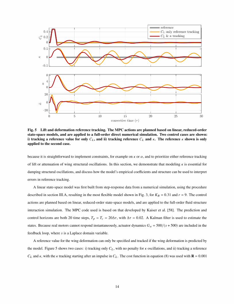
Fig. 5 Lift and deformation reference tracking. The MPC actions are planned based on linear, reduced-orderstate-space models, and are applied to a full-order direct numerical simulation. Two control cases are shown:i) tracking a reference value for only 𝐶𝐿 , and ii) tracking reference 𝐶𝐿 and ^. The reference ^ shown is onlyapplied to the second case.

because it is straightforward to implement constraints, for example on ^ or 𝛼, and to prioritize either reference tracking

of lift or attenuation of wing structural oscillations. In this section, we demonstrate that modeling ^ is essential for

damping structural oscillations, and discuss how the model’s empirical coefficients and structure can be used to interpret

errors in reference tracking.

A linear state-space model was first built from step-response data from a numerical simulation, using the procedure

described in section III.A, resulting in the most flexible model shown in Fig. 3, for 𝐾𝐵 = 0.31 and 𝑟 = 9. The control

actions are planned based on linear, reduced-order state-space models, and are applied to the full-order fluid structure

interaction simulation. The MPC code used is based on that developed by Kaiser et al. [58]. The prediction and

control horizons are both 20 time steps, 𝑇𝑝 = 𝑇𝑐 = 20Δ𝜏, with Δ𝜏 = 0.02. A Kalman filter is used to estimate the

states. Because real motors cannot respond instantaneously, actuator dynamics 𝐺𝑎 = 500/(𝑠 + 500) are included in the

feedback loop, where 𝑠 is a Laplace domain variable.

A reference value for the wing deformation can only be specified and tracked if the wing deformation is predicted by

the model. Figure 5 shows two cases: i) tracking only 𝐶𝐿 , with no penalty for ^ oscillations, and ii) tracking a reference

𝐶𝐿 and ^, with the ^ tracking starting after an impulse in 𝐶𝐿 . The cost function in equation (8) was used with R = 0.001

14

Fig. 6 The maximum wing deformation depends strongly on the duration of the reference 𝐶𝐿 step. (left)Reference 𝐶𝐿 is increased, held, and decreased with three different rates of increase and hold time. If the holdtime is too short, the system is unable to respond quickly enough. As the hold time increases, the maximum ^

and 𝛼 also increase. (right) By choosing reference 𝐶𝐿 with short enough hold times, moderate constraints onmaximum ^ do not affect reference tracking accuracy.

and

Q1 =

1 0

0 0

and Q2 =

1 0

0 10

, (13)

where Q1 is used during periods with non-zero reference 𝐶𝐿 , and Q2 is applied for the second case to minimize

structural vibrations when the magnitude of the reference 𝐶𝐿 is zero. The first case, where only a reference for 𝐶𝐿

is specified, shows that wing vibrations from rapid maneuvers persist for a long time after the maneuver, despite the

well-controlled lift. When a reference deformation is specified, vibrations are quickly attenuated. There is some trade

off in lift tracking performance when deformation is included in the MPC cost function. This model makes it possible to

tune the optimization weights and control constraints to decide the right trade-off for a given control application, rather

than relying only on lift tracking.

Limiting the maximum wing deformation is another goal of deformation control, to avoid damage from large stresses.

Similar to the model described in Fig. 4 and equation (12), the model used in this section has significant contributions to

𝐶𝐿 from ¥𝛼, due to added mass; however, the largest contribution to ^ is from 𝛼. Shown in Fig. 6 (left), this results in

small deformations when the reference 𝐶𝐿 is stepped-up and then stepped back down in a short time, because the MPC

15

Fig. 7 For systems with significant added mass effects on𝐶𝐿 , constraints on deformation decrease performancewhen 𝐶𝐿 is held constant, but does not affect accuracy at the beginning of maneuvers.

optimization is able to use added mass forces to generate most of the increase in 𝐶𝐿 . However, if the high reference 𝐶𝐿

is held for longer, there is no longer added mass due to acceleration, and the angle of attack must increase to sustain the

𝐶𝐿 at the reference value. When the reference maneuver is too rapid, the controller is unable to respond quickly enough.

An understanding of the relative contributions from added mass and angle of attack can be used to balance the

need for constraining deformation with desired trajectories. In Fig. 6 (right), the ^ constraint does not affect shorter

maneuvers, but leads to significant error for a longer maneuver. In this regime, constraining ^ effectively also constrains

𝛼. As constraints on deformation become more aggressive, the lift of the controlled system falter earlier, as shown in

Fig. 7.

V. DiscussionIn this work, we describe a method for obtaining accurate low order, linear state space aeroelastic models for

control. The method uses lift and deformation data from an impulse response to construct the model, providing accurate

predictions without requiring information about the surrounding flow field or wing structural properties. Interpretable

coefficients relating to added mass, lift slope, and transient effects are built in to the model, providing insights about

the underlying physics. The remaining dynamics are modeled using ERA, which accurately captures the transients

dynamics due to the viscous wake. The resulting model is low dimensional and captures the dominant dynamics,

extending rigid state-space aerodynamic models [45] to account for wing flexibility. Two variations of the modeling

method were presented. One variation integrates the training data, and is recommended for cases where the amplitude

16

of the bending modes is separated by several orders of magnitude. The other variation is recommended for cases where

the wing bending modes are strongly dominant over signal noise in the training data.

These models are well-suited for use with standard control techniques, which is demonstrated using MPC to track

an aggressive reference lift while attenuating oscillations in leading edge curvature. These state-space models allow

analysis and control design in both the time and frequency domains, including identification of resonant frequencies

of the flexible structure. Because the wing deformation can be predicted, wing vibrations or flutter can be actively

controlled by modulating only the angle of attack.

There are several interesting directions in which this work may be extended. Although the results here were

demonstrated for two-dimensional wings in simulations, the modeling procedure should generalize to three-dimensional

wings and data from experiments. For experimental data, it may be necessary to employ the observer-Kalman filter

identification (OKID) approach [59], which has been demonstrated for the identifiation of rigid unsteady aerodynamic

models from data [40, 45]. It will also be important to extend these models to handle larger amplitude maneuvers, either

by combining multiple linear models using LPV models [46] or by including nonlinear terms in the model.

Curvature was used as the measure of deformation in this paper because the data was based on a simulation

without a well-defined plate thickness. In real-world and experimental settings, strain may be a more appropriate

deformation observable due to ease of measurement. Expanding the modeling algorithm to include a preprocessing step

of determining the optimal strain sensor location may be of value [60]. Another possible extension of this modeling

method is to include coefficient of thrust as an observable, giving a more complete picture of the forces on the wing,

making the work more relevant for flapping and hovering flight.

While this data-driven modelling method can be used in regimes relevant to aircraft or wind turbines, its development

was particularly motivated by development of MAVs and to investigate control strategies used in animal flight, due

to the inclusion of viscous effects. Managing wing loading while increasing efficiency at small scales is an ongoing

challenge, which these models are designed to address. Animals achieve impressive maneuverability and stability with

limited computation, and one goal of low-order models is to enable similar performance in engineered vehicles. This

modeling framework fills a need for control-oriented models for flying or swimming animals and for micro air vehicles

(MAVs), both of which rely on viscous and unsteady forces, with passive wing or fin flexibility playing a major role in

efficient locomotion [61–64].

17

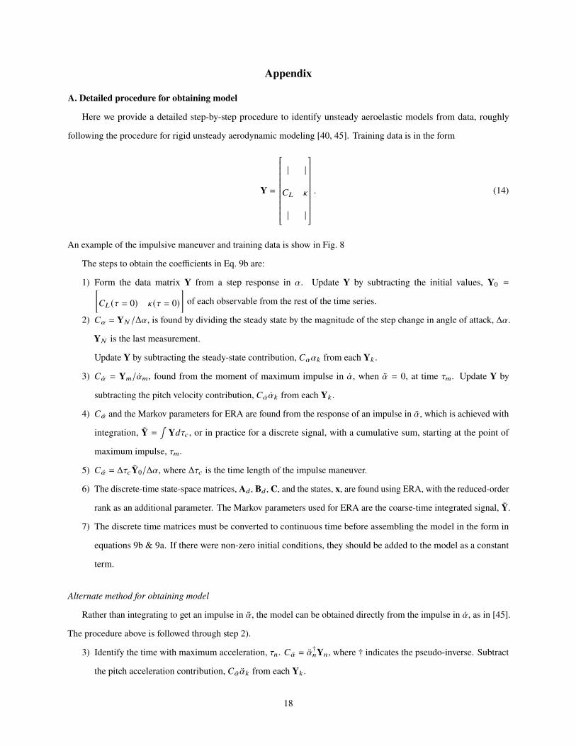
Appendix

A. Detailed procedure for obtaining model

Here we provide a detailed step-by-step procedure to identify unsteady aeroelastic models from data, roughly

following the procedure for rigid unsteady aerodynamic modeling [40, 45]. Training data is in the form

Y =

| |

𝐶𝐿 ^

| |

. (14)

An example of the impulsive maneuver and training data is show in Fig. 8

The steps to obtain the coefficients in Eq. 9b are:

1) Form the data matrix Y from a step response in 𝛼. Update Y by subtracting the initial values, Y0 =[𝐶𝐿 (𝜏 = 0) ^(𝜏 = 0)

]of each observable from the rest of the time series.

2) 𝐶𝛼 = Y𝑁 /Δ𝛼, is found by dividing the steady state by the magnitude of the step change in angle of attack, Δ𝛼.

Y𝑁 is the last measurement.

Update Y by subtracting the steady-state contribution, 𝐶𝛼𝛼𝑘 from each Y𝑘 .

3) 𝐶 ¤𝛼 = Y𝑚/ ¤𝛼𝑚, found from the moment of maximum impulse in ¤𝛼, when ¥𝛼 = 0, at time 𝜏𝑚. Update Y by

subtracting the pitch velocity contribution, 𝐶 ¤𝛼 ¤𝛼𝑘 from each Y𝑘 .

4) 𝐶 ¥𝛼 and the Markov parameters for ERA are found from the response of an impulse in ¥𝛼, which is achieved with

integration, Y =∫

Y𝑑𝜏𝑐 , or in practice for a discrete signal, with a cumulative sum, starting at the point of

maximum impulse, 𝜏𝑚.

5) 𝐶 ¥𝛼 = Δ𝜏𝑐Y0/Δ𝛼, where Δ𝜏𝑐 is the time length of the impulse maneuver.

6) The discrete-time state-space matrices, A𝑑 , B𝑑 , C, and the states, x, are found using ERA, with the reduced-order

rank as an additional parameter. The Markov parameters used for ERA are the coarse-time integrated signal, Y.

7) The discrete time matrices must be converted to continuous time before assembling the model in the form in

equations 9b & 9a. If there were non-zero initial conditions, they should be added to the model as a constant

term.

Alternate method for obtaining model

Rather than integrating to get an impulse in ¥𝛼, the model can be obtained directly from the impulse in ¤𝛼, as in [45].

The procedure above is followed through step 2).

3) Identify the time with maximum acceleration, 𝜏𝑛. 𝐶 ¥𝛼 = ¥𝛼†𝑛Y𝑛, where † indicates the pseudo-inverse. Subtract

the pitch acceleration contribution, 𝐶 ¥𝛼 ¥𝛼𝑘 from each Y𝑘 .

18

Fig. 8 An impulse in ¤𝛼 is used to generate training data used for the system identification algorithm. The datashown is for 𝐾𝐵 = 0.31, and represents a short time window during and after the impulse. Data should be takenuntil all transients and wing bending cease.

4) The Markov parameters,Y, are the signal Y sampled at intervals of the coarse time step, Δ𝜏𝑐 , starting at the time

of maximum impulse, 𝜏𝑚.

5) 𝐶 ¤𝛼 = Δ𝜏𝑐Y0/Δ𝛼.

6) A𝑑 , B𝑑 , C & x, are found using ERA with Y, and then converted to continuous time and assembled into the form

in equations 10 & 9b. If there were non-zero initial conditions, they should be added to the model as a constant

term.

B. Fluid-structure interaction model

We performed direct numerical simulation of a flow over a two-dimensional thin deforming plate with a strongly-

coupled immersed boundary projection method [19]. The incompressible Navier–Stokes equation for the fluid was

discretized in the vorticity-streamfunction form [65] with accurate surface stresses and forces to enforce the boundary

condition at the plate [66]. At the far-field boundaries, uniform flow with free stream velocity 𝑈∞ was prescribed.

The solver uses an explicit Adam-Bashforth method and an implicit Crank-Nicolson scheme for discretization of the

advective and viscous terms of the Navier–Stokes equation, respectively. To speed up the computations, a multi-domain

technique with five grid levels was implemented [67]. The finest domain was fixed at −0.2 ≤ 𝑥/𝑐 ≤ 1.8,−1 ≤ 𝑦/𝑐 ≤ 1

with a grid spacing of Δ𝑥/𝑐 ≈ 0.0077. Here 𝑐 is the length of the plate. The Reynolds number for all the simulations in

this work is 𝑅𝑒 ≡ 𝑈∞𝑐/a = 100, where a is the kinematic viscosity.

The Euler-Bernoulli equation for the plate was discretized using a co-rotational finite element formulation [68]. This

formulation enables arbitrary large displacements and rotations by attaching a local coordinate frame to each element.

19

The plate was discretized into 65 elements with the leading edge placed at (𝑥/𝑐, 𝑦/𝑐) = (0, 0).

Data accessibilityThe code used in this work is available at https://github.com/mhickner/aeroelastic-ss-model, including sample data

which can be used to generate the models shown in section IV.

AcknowledgementsThe authors acknowledge support from the Air Force Office of Scientific Research (AFOSR FA9550-19-1-0386)

and the National Science Foundation AI Institute in Dynamic Systems (Grant No. 2112085).

References[1] Fernández-Gutiérrez, D., and Van Rees, W. M., “Effect of leading-edge curvature actuation on flapping fin performance,” J.

Fluid Mech, Vol. 921, 2021, p. 22. https://doi.org/10.1017/jfm.2021.469, URL https://doi.org/10.1017/jfm.2021.469.

[2] Hang, H., Heydari, S., Costello, J. H., and Kanso, E., “Active tail flexion in concert with passive hydrodynamic forces improvesswimming speed and efficiency,” arXiv, 2021. URL http://arxiv.org/abs/2104.11869.

[3] Daniel, T. L., “Forward flapping flight from flexible fins,” Canadian journal of zoology, Vol. 66, No. 3, 1988, pp. 630–638.

[4] Fish, F. E., and Hui, C. A., “Dolphin swimming–a review,”Mammal Review, Vol. 21, No. 4, 1991, pp. 181–195.

[5] Dickinson, M. H., and G otz, K. G., “The wake dynamics and flight forces of the fruit fly Drosophila melanogaster,” TheJournal of Experimental Biology, Vol. 199, 1996, pp. 2085–2104.

[6] Fish, F. E., “Transitions from drag-based to lift-based propulsion in mammalian swimming,” American Zoologist, Vol. 36,No. 6, 1996, pp. 628–641.

[7] Dickinson, M. H., Lehmann, F. O., and Sane, S. P., “Wing rotation and the aerodynamic basis of insect flight,” Science, Vol.284, No. 5422, 1999, pp. 1954–1960.

[8] Birch, J., and Dickinson, M., “Spanwise flow and the attachment of the leading-edge vortex on insect wings.” Nature, Vol. 412,2001, pp. 729–733.

[9] Combes, S. A., and Daniel, T. L., “Shape, flapping and flexion: wing and fin design for forward flight,” The Journal ofExperimental Biology, Vol. 204, 2001, pp. 2073–2085.

[10] Sane, S. P., and Dickinson, M. H., “The control of flight force by a flapping wing: lift and drag production,” The Journal ofExperimental Biology, Vol. 204, 2001, pp. 2607–2626.

[11] Liao, J. C., Beal, D. N., Lauder, G. V., and Triantafyllou, M. S., “Fish exploiting vortices decrease muscle activity,” Science,Vol. 302, No. 5650, 2003, pp. 1566–1569.

[12] Tytell, E. D., and Lauder, G. V., “The hydrodynamics of eel swimming I. Wake structure,” The Journal of Experimental Biology,Vol. 207, 2004, pp. 1825–1841.

[13] Lauder, G. V., and Tytell, E. D., “Hydrodynamics of undulatory propulsion,” Fish physiology, Vol. 23, 2005, pp. 425–468.

[14] Wang, Z. J., “Dissecting Insect Flight,” Annual Review of Fluid Mechanics, Vol. 37, 2005, pp. 183–210.

[15] Hedenström, A., Johansson, L., Wolf, M., Von Busse, R., Winter, Y., and Spedding, G., “Bat flight generates complexaerodynamic tracks,” Science, Vol. 316, No. 5826, 2007, pp. 894–897.

[16] Peng, J., and Dabiri, J. O., “The ‘upstream wake’ of swimming and flying animals and its correlation with propulsive efficiency,”The Journal of Experimental Biology, Vol. 211, 2008, pp. 2669–2677.

[17] Riskin, D. K., Willis, D. J., Iriarte-Díaz, J., Hedrick, T. L., Kostandov, M., Chen, J., Laidlaw, D. H., Breuer, K. S., and Swartz,S. M., “Quantifying the complexity of bat wing kinematics,” Journal of Theoretical Biology, Vol. 254, No. 3, 2008, pp. 604–615.

[18] Dabiri, J. O., “Optimal vortex formation as a unifying principle in biological propulsion,” Annual Review of Fluid Mechanics,Vol. 41, 2009, pp. 17–33.

20

[19] Shelley, M. J., and Zhang, J., “Flapping and bending bodies interacting with fluid flows,” Annual Review of Fluid Mechanics,Vol. 43, 2011, pp. 449–465.

[20] Wu, T. Y., “Fish swimming and bird/insect flight,” Annual Review of Fluid Mechanics, Vol. 43, 2011, pp. 25–58.

[21] Leftwich, M. C., Tytell, E. D., Cohen, A. H., and Smits, A. J., “Wake structures behind a swimming robotic lamprey with apassively flexible tail,” The Journal of Experimental Biology, Vol. 215, No. 3, 2012, pp. 416–425.

[22] Nawroth, J. C., Lee, H., Feinberg, A. W., Ripplinger, C. M., McCain, M. L., Grosberg, A., Dabiri, J. O., and Parker, K. K., “Atissue-engineered jellyfish with biomimetic propulsion,” Nature Biotechnology, Vol. 30, 2012, pp. 792–797.

[23] Floryan, D., and Rowley, C. W., “Distributed flexibility in inertial swimmers,” Journal of Fluid Mechanics, Vol. 888, 2020.https://doi.org/10.1017/jfm.2020.49.

[24] Peskin, C. S., “The immersed boundary method,” Acta Numerica, Vol. 11, 2002, p. 479–517. https://doi.org/10.1017/S0962492902000077.

[25] Mittal, R., and Iaccarino, G., “Immersed boundary methods,” Annual Review of Fluid Mechanics, Vol. 37, 2005, pp. 239–261.https://doi.org/10.1146/annurev.fluid.37.061903.175743, URL https://www-annualreviews-org.offcampus.lib.washington.edu/doi/abs/10.1146/annurev.fluid.37.061903.175743.

[26] Goza, A., and Colonius, T., “A strongly-coupled immersed-boundary formulation for thin elastic structures,” Journal ofComputational Physics, Vol. 336, 2017, pp. 401–411. https://doi.org/10.1016/j.jcp.2017.02.027, URL www.elsevier.com/locate/jcp.

[27] Albano, E., and Rodden, W. P., “A doublet-lattice method for calculating lift distributions on oscillating surfaces in subsonicflows,” AIAA Journal, Vol. 7, No. 11, 1969, pp. 2192a–2192a. https://doi.org/10.2514/3.55530.

[28] Kim, D.-K., Lee, J.-S., Lee, J.-Y., and Han, J.-H., “An aeroelastic analysis of a flexible flapping wing using modified striptheory,” Active and Passive Smart Structures and Integrated Systems 2008, Vol. 6928, 2008. https://doi.org/10.1117/12.776137.

[29] Wang, Y., Zhao, X., Palacios, R., and Otsuka, K., “Aeroelastic Simulation of High-Aspect Ratio Wings with IntermittentLeading-Edge Separation,” AIAA JOURNAL, 2021. https://doi.org/10.2514/1.J060909, URL https://doi.org/10.2514/1.J060909.

[30] Fasel, U., Tiso, P., Keidel, D., and Ermanni, P., “Concurrent Design and Flight Mission Optimization of Morphing AirborneWind Energy Wings,” AIAA Journal, Vol. 59, No. 4, 2021, pp. 1254–1268.

[31] Hesse, H., and Palacios, R., “Reduced-order aeroelastic models for dynamics of maneuvering flexible aircraft,” AIAA Journal,Vol. 52, No. 8, 2014, pp. 1717–1732. https://doi.org/10.2514/1.J052684, URL http://arc.aiaa.org.

[32] Murua, J., Palacios, R., and Graham, J. M. R., “Applications of the unsteady vortex-lattice method in aircraft aeroelasticity andflight dynamics,” Progress in Aerospace Sciences, Vol. 55, 2012, pp. 46–72. https://doi.org/10.1016/j.paerosci.2012.06.001.

[33] Brockett, R. W., “Volterra Series and Geometric Control Theory,” Automatica, Vol. 12, 1976, pp. 167–176.

[34] Balajewicz, M., and Dowell, E., “Reduced-Order Modeling of Flutter and Limit-Cycle Oscillations Using the Sparse VolterraSeries,” Journal of Aircraft, Vol. 49, No. 6, 2012, pp. 1803–1812. https://doi.org/10.2514/1.C031637, URL http://arc.aiaa.org.

[35] Fonzi, N., Brunton, S. L., and Fasel, U., “Data-driven nonlinear aeroelastic models of morphing wings for control: Data-drivennonlinear aeroelastic models,” Proceedings of the Royal Society A: Mathematical, Physical and Engineering Sciences, Vol. 476,No. 2239, 2020. https://doi.org/10.1098/rspa.2020.0079rspa20200079.

[36] Artola, M., Goizueta, N., Wynn, A., and Palacios, R., “Aeroelastic Control and Estimation with a Minimal NonlinearModal Description,” AIAA Journal, Vol. 59, No. 7, 2021, pp. 2697–2713. https://doi.org/10.2514/1.j060018, URL https://doi.org/10.2514/1.J060018.

[37] Lucia, D. J., Beran, P. S., and Silva, W. A., “Aeroelastic system development using proper orthogonal decomposition andvolterra theory,” Journal of Aircraft, Vol. 42, No. 2, 2005, pp. 509–518. https://doi.org/10.2514/1.2176.

[38] Dullerud, G. E., and Paganini, F., A course in robust control theory: A convex approach, Texts in Applied Mathematics,Springer, Berlin, Heidelberg, 2000.

[39] Skogestad, S., and Postlethwaite, I.,Multivariable feedback control: analysis and design, 2nd ed., John Wiley & Sons, Inc.,Hoboken, New Jersey, 2005.

[40] Brunton, S. L., Rowley, C. W., and Williams, D. R., “Reduced-order unsteady aerodynamic models at low Reynolds numbers,”Journal of Fluid Mechanics, Vol. 724, 2013, pp. 203–233. https://doi.org/10.1017/jfm.2013.163.

[41] Eldredge, J. D., and Jones, A. R., “Leading-edge vortices: mechanics and modeling,” Annual Review of Fluid Mechanics,Vol. 51, 2019, pp. 75–104.

21

[42] Theodorsen, T., “General Theory of Aerodynamic Instability and the Mechanism of Flutter,” Technical Report, NACA, , No.496, 1935, pp. 291–311.

[43] Wagner, H., “Über die Entstehung des dynamischen Auftriebes von Tragflügeln,” ZAMM - Journal of Applied Mathematics andMechanics / Zeitschrift für Angewandte Mathematik und Mechanik, Vol. 5, No. 1, 1925, pp. 17–35. https://doi.org/10.1002/zamm.19250050103.

[44] Brunton, S. L., and Rowley, C. W., “Empirical state-space representations for Theodorsen’s lift model,” Journal of Fluids andStructures, Vol. 38, 2013, pp. 174–186. https://doi.org/10.1016/j.jfluidstructs.2012.10.005, URL http://dx.doi.org/10.1016/j.jfluidstructs.2012.10.005.

[45] Brunton, S. L., Dawson, S. T., and Rowley, C.W., “State-spacemodel identification and feedback control of unsteady aerodynamicforces,” Journal of Fluids and Structures, Vol. 50, 2014, pp. 253–270. https://doi.org/10.1016/j.jfluidstructs.2014.06.026.

[46] Hemati, M. S., Dawson, S. T., and Rowley, C. W., “Parameter-varying aerodynamics models for aggressive pitching-responseprediction,” AIAA Journal, Vol. 55, No. 3, 2017, pp. 693–701. https://doi.org/10.2514/1.J055193.

[47] Nardini, M., Illingworth, S. J., and Sandberg, R. D., “Reduced-order modeling and feedback control of a flexible wing at lowReynolds numbers,” Journal of Fluids and Structures, Vol. 79, 2018, pp. 137–157. https://doi.org/10.1016/j.jfluidstructs.2018.02.003, URL https://doi.org/10.1016/j.jfluidstructs.2018.02.003.

[48] Juang, J.-N., and Pappa, R. S., “An eigensystem realization algorithm for modal parameter identification and model reduction,”Journal of Guidance, Control, and Dynamics, Vol. 8, No. 5, 1985, pp. 620–627. https://doi.org/10.2514/3.20031, URLhttps://arc.aiaa.org/doi/10.2514/3.20031.

[49] Garrick, I. E., “On Some Reciprocal Relations in the Theory of Nonstationary Flow,” NACA Report 629, 1938, pp. 347–350.

[50] Jones, R. T., “Operational treatment of the nonuniform-lift theory in airplane dynamics,” NACA, , No. Technical Note 667,1938, pp. 0–11. URL http://hdl.handle.net/2060/19930081472.

[51] Leishman, J. G., Principles of Helicopter Aerodynamics, Cambridge University Press, 2006.

[52] Vepa, R., “Finite state modeling of aeroelastic systems,” NASA Contracter Report, Vol. CR-2779, No. February 1977, 1977.URL http://ntrs.nasa.gov/search.jsp?R=19770012545.

[53] Ma, Z., Ahuja, S., and Rowley, C. W., “Reduced-order models for control of fluids using the eigensystem realization algorithm,”Theoretical and Computational Fluid Dynamics 2010 25:1, Vol. 25, No. 1, 2010, pp. 233–247. https://doi.org/10.1007/S00162-010-0184-8.

[54] Eldredge, J. D., Wang, C., and OL, M. V., “A computational study of a canonical pitch-up, pitch-down wing maneuver,” AIAAPaper 2009-3687, 39th Fluid Dynamics Conference, June 2009.

[55] OL, M. V., Altman, A., Eldredge, J. D., Garmann, D. J., and Lian, Y., “Résumé of the AIAA FDTC Low Reynolds NumberDiscussion Group’s canonical cases,” 48th AIAA Aerospace Sciences Meeting Including the New Horizons Forum and AerospaceExposition, , No. January, 2010. https://doi.org/10.2514/6.2010-1085.

[56] Cheng, B., Deng, X., and Hedrick, T. L., “The mechanics and control of pitching manoeuvres in a freely flying hawkmoth(Manduca sexta),” Journal of Experimental Biology, Vol. 214, No. 24, 2011, pp. 4092–4106. https://doi.org/10.1242/jeb.062760.

[57] Combes, S. A., and Daniel, T. L., “Flexural stiffness in insect wings II. Spatial distribution and dynamic wing bending,” Journalof Experimental Biology, Vol. 206, No. 17, 2003, pp. 2989–2997. https://doi.org/10.1242/jeb.00524.

[58] Kaiser, E., Kutz, J. N., and Brunton, S. L., “Sparse identification of nonlinear dynamics for model predictive control in thelow-data limit,” Proceedings of the Royal Society A: Mathematical, Physical and Engineering Sciences, Vol. 474, No. 2219,2018. https://doi.org/10.1098/rspa.2018.0335.

[59] Juang, J.-N., Phan, M., Horta, L. G., and Longman, R. W., “Identification of Observer/Kalman Filter Markov Parameters:Theory and Experiments,” NASA Technical Memorandum, , No. 104069, 1991.

[60] Mohren, T. L., Daniel, T. L., Brunton, S. L., and Brunton, B. W., “Neural-inspired sensors enable sparse, efficient classificationof spatiotemporal data,” Proceedings of the National Academy of Sciences, Vol. 115, No. 42, 2018, pp. 10564–10569.

[61] Daniel, T. L., and Combes, S. A., “Flexible wings and fins: Bending by inertial or fluid-dynamic forces?” Integrative andComparative Biology, Vol. 42, 2002, pp. 1044–1049. https://doi.org/10.1093/icb/42.5.1044.

[62] Mountcastle, A. M., and Combes, S. A., “Wing flexibility enhances load-lifting capacity in bumblebees,” Proceedingsof the Royal Society B: Biological Sciences, Vol. 280, No. 1759, 2013. https://doi.org/10.1098/rspb.2013.0531, URLhttp://rspb.royalsocietypublishing.org.

22

[63] Song, A., Tian, X., Israeli, E., Galvao, R., Bishop, K., Swartz, S., and Breuer, K., “Aeromechanics of membrane wings withimplications for animal flight,” AIAA Journal, Vol. 46, No. 8, 2008, pp. 2096–2106. https://doi.org/10.2514/1.36694, URLhttp://arc.aiaa.org.

[64] Tytell, E. D., Leftwich, M. C., Hsu, C. Y., Griffith, B. E., Cohen, A. H., Smits, A. J., Hamlet, C., and Fauci, L. J., “Role of bodystiffness in undulatory swimming: Insights from robotic and computational models,” Physical Review Fluids, Vol. 1, No. 7,2016, p. 073202. https://doi.org/10.1103/PHYSREVFLUIDS.1.073202.

[65] Taira, K., and Colonius, T., “The immersed boundary method: a projection approach,” Journal of Computational Physics, Vol.225, 2007, pp. 2118–2137.

[66] Goza, A., Liska, S., Morley, B., and Colonius, T., “Accurate computation of surface stresses and forces with immersed boundarymethods,” Journal of Computational Physics, Vol. 321, 2016, pp. 860–873.

[67] Colonius, T., and Taira, K., “A fast immersed boundary method using a nullspace approach and multi-domain far-field boundaryconditions,” Computer Methods in Applied Mechanics and Engineering, Vol. 197, 2008, pp. 2131–2146.

[68] Criesfield, M., “Non-linear finite element analysis of solids and structures, vol. 1,” , 1991.

23