Data dissemination using the energy map

Data Dissemination Using the Energy Map

Max do V. Machado1, Olga Goussevskaia1, Raquel A.F. Mini2, Cristiano G. Rezende1

Antonio A.F. Loureiro1, Geraldo R Mateus1 and Jose Marcos Nogueira1

1Federal University of Minas Gerais, Brazil2Pontifical University Catholic of Minas Gerais, Brazil

E-mail:{maxm,olga,raquel,rezende,loureiro,mateus,jmarcos }@dcc.ufmg.br

Abstract

One of the most important resources in wireless sensornetworks is energy, since, in general, batteries cannot berecharged. The information about the amount of energyavailable at each part of the network is called the energymap and can be explored by routing algorithms. In thiswork, a new routing algorithm for wireless sensor networksis proposed. The key idea is to combine concepts presentedin trajectory-based forwarding with the information pro-vided by the energy map to determine routes in a dynamicfashion. Simulation results revealed that the energy spentwith routing activity can be concentrated on nodes with highenergy reserves, whereas low-energy nodes can use theirenergy only to perform sensing activity. In this manner, par-titions of the network due to nodes that ran out of energy canbe significantly delayed and the network lifetime extended.

1 Introduction

Wireless sensor networks (WSNs) pose new researchchallenges related to the design of algorithms, network pro-tocols, and software that will enable the development of ap-plications based on sensor devices [2], [6]. In WSNs, theenergy expenditure in data communication is much morecompared to data processing. Thus, any communication so-lution to this kind of network must be power efficient toextend its lifetime.

In WSNs, data communication, from the point of view ofthe communicating entities, can be divided into three cases:from sink node to sensor nodes, from sensor nodes to sinknode, and among neighbor nodes. In each case, it is possibleto have a different goal. Data communication from a sinknode to a set of sensor nodes is often used to disseminate apiece of information that is important to those nodes. Forinstance, a sink node could disseminate a new interest of adata to be sensed to a set of nodes. This kind of data com-

munication is often called data dissemination. Data com-munication from sensor nodes to a sink node is used to sendthe sensed data collected by the sensors to a monitoringapplication. Finally, data communication among neighbornodes often happens when some kind of cooperation amongnodes is needed. In this work, we are interested in data dis-semination from sink node to sensor nodes.

In [10], Niculescu and Nath propose theTrajectoryBased Forwarding(TBF) algorithm that is a technique todisseminate packets from a sink node to a set of nodes alonga predefined curve in a wireless dense network. In TBF,the trajectory is embedded in each packet and the interme-diate nodes make the forwarding decisions based on theirdistances from the desired trajectory. The innovation of thisapproach comes from the definition and treatment of routepaths as a continuous function as opposed to a discrete setof points. Therefore, TBF is suitable for large scale, densewireless ad-hoc and sensor networks.

In WSNs, the data communication cost can be repre-sented by the energy consumption. The information aboutthe amount of energy available at each part of the networkis called the energy map. This map can be represented byan image in tones of gray. The darker the tone of gray, thelesser is the amount of energy available at that network re-gion. Knowing which are the areas of low energy can beuseful in many activities of a WSN, such as routing, recon-figuration, data fusion, or network management algorithms.For instance, a routing protocol can make a better use ofthe energy reserves if it selectively chooses routes that usenodes with more remaining energy. The important pointhere is that the map can be useful in prolonging the networklifetime. In this work, a prediction-based approach to con-struct the energy map, presented in [8], is going to be used.

Most of the issues related to determining and specifyingthe trajectory for TBF are still open topics of research. Inthis work, we propose a method not only for representingthe trajectories, but also for specifying them dynamicallybased on the energy map. The main idea is to select a set ofnodes in the network that are most suitable for forwarding

the packets sent by the sink and to find the best set of curvespassing through or near these selected points. Multiple lin-ear regressing [9] was used to perform the curve fitting. Thetrajectory generation procedure was designed to be directedby the requirements of the application, which can aim tomaximize the amount of energy available at the forwardingnodes, or maximize the percentage of nodes the informationdisseminated by the sink has to reach.

Moreover, we propose a new forwarding mechanism,called TBF+, which is much more effective in terms ofenergy consumption and presents a more robust behaviorin a dynamic topology scenario, where nodes can period-ically go into sleeping mode. Results show that the en-ergy spent with data communication can be concentrated onthose nodes that have high-energy reserves, whereas low-energy nodes can use their energy only in other network ac-tivities such as sensing activity and reception of informationaddressed to them. Therefore, partitions of the network dueto nodes that ran out of energy can be significantly delayedand the network lifetime can be extended.

The rest of this work is organized as follows. Section 2shows the related work. The two parts of our proposal, thetrajectory generation process and the TBF+, are presentedin Section 3 and 4, respectively. In Section 5, we show thesimulation process and analyze the experimental results ofthe TBF+. Section 6 presents an analytical model for mea-suring our protocol performance bounds. Finally, Section 7shows the conclusions and the future directions of this work.

2 Related work

Several different routing protocols for WSNs have beenproposed in the literature [1]. Due to the nature of thesenetworks, the basic requirements for routing techniques arescalability and robustness for data dissemination [3]. Thealgorithms for these networks have to be designed aiming toextend the network lifetime and, therefore, have to provideboth robust communication mechanisms and efficient en-ergy consumption. Some examples of the existing data dis-semination techniques are Directed Diffusion and TBF (It isgoing to be analyzed in Section 4). In [4], [5], Intanagonwi-wat et. al propose the Directed Diffusion, a framework fordata communication in sensor networks. This protocol aimsto establish efficient communication between sensors andthe sink node. The operation of Directed Diffusion can beshortly described as follows. The sink node disseminatesthroughout the network a sensing task or an interest andthe intermediate nodes propagate the interest over the net-work using local interactions and aggregating the receivedevents into a unique event, in order to reduce the number oftransmissions and the amount of data stored by the network.The propagation route of the interest determines the reversepath for the locally collected data which matches with the

interest. This dissemination creates a gradient based on thetopology of the network, which becomes directed by events.The gradient guarantees that the collected data uses uniquepaths when routed back to the sink.

The information about the amount of energy availableat each part of the network is very useful in WSNs. Thework presented in [8] focuses on proposing mechanisms topredict the energy consumption of a sensor node in order toconstruct the energy map of a WSN. There are situations inwhich the node can predict its energy consumption based onits own past history. If a sensor can predict efficiently theamount of energy it will dissipate in the future, it will not benecessary to transmit frequently its available energy. Thisnode can just send one message with its available energyand the parameters of the model that describes its energydissipation. With this information, the monitoring node canupdate often its local information about the available energyof this node. Simulation results presented in [8] showedthat prediction-based models decrease the amount of energynecessary to construct the energy map.

3 Dynamic Trajectory Generation

In [10], Niculescu and Nath suggest a number of choicesfor representing a trajectory. Some of these methods arelisted below:

• Functional(e.g.,y = f(x));

• Equational(e.g.,x2 + y2 = r2);

• Parametric(e.g.,x = X(t), y = Y (t));

• Complex trajectories: can be specified as a number ofsimple components such as Fourier components;

• Recursive representation: suitable for multicast for-warding, where the entire distribution tree has to bespecified; however, would work only in certain cases,when such a tree has a regular shape and its recursiverepresentation can be sufficiently compact.

In spite of having given several insights into the prob-lems that might arise during the process of determining andspecifying a forwarding trajectory, in [10] it is not addressedthis issue, specially for the problem of how and based onwhat kind of information the trajectory should be deter-mined.

In this work, we propose a method not only for repre-senting the trajectories, but also for specifying them dynam-ically based on the energy map. The main idea is to selecta set of nodes in the network that are most suitable for for-warding the packets sent by the sink and to find the best setof curves passing through or near these selected points. Thechoice of the best set of curves can be based on different

criteria, such as the amount of energy available at the for-warding nodes, or the percentage of nodes the informationdisseminated by the sink is supposed to reach.

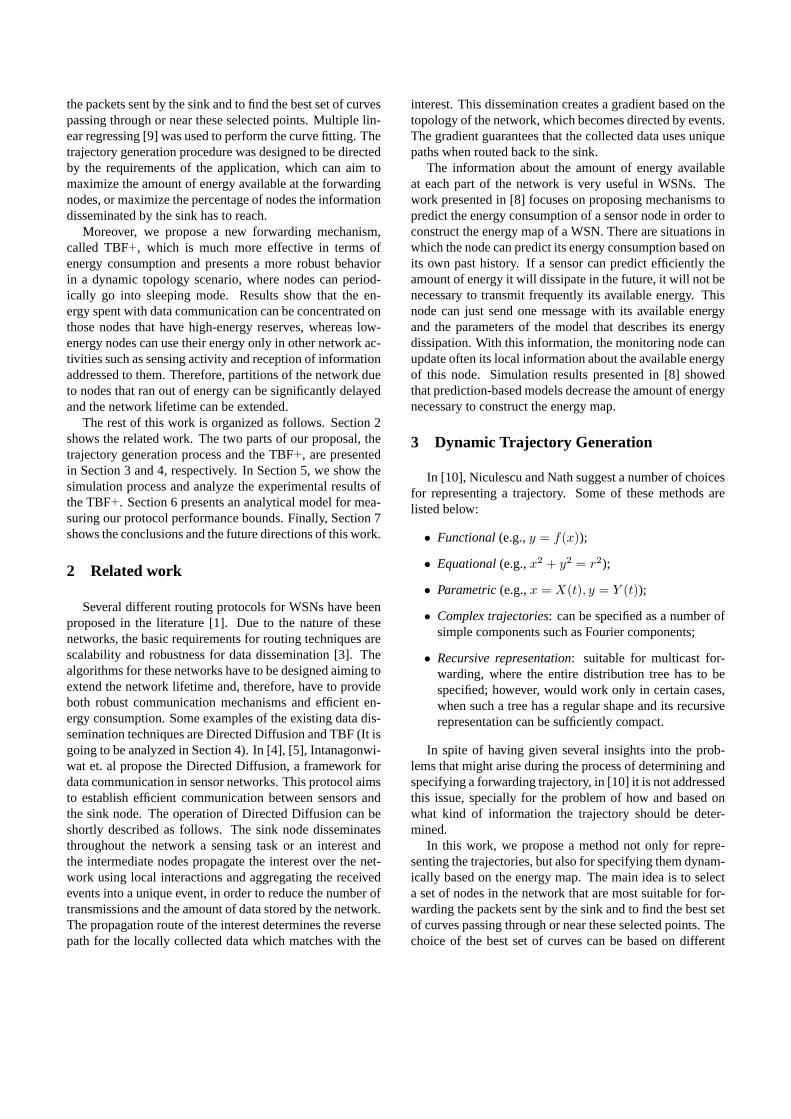
Since we intend to base the trajectory generation onthe energy map, we decided to use functional and equa-tional representations, allowing more than one trajectory tobe encoded at each forwarded packet. We consider thesetwo types of representation expressive enough to guaranteethe flexibility required to forward packets through areas ofgreater energy reserves. It is worth noting that low energyareas can change along time due to localized event occur-rences or other factors causing irregular energy distributionover the network. The process of generating a set of trajec-tories is illustrated in Figure 1, as discussed in the rest ofthis section.

3.1 Point/Node Selection

The first step in the trajectory generation process is thepoint or node selection, as shown in Figure 1, pointA. Inorder to perform the curve fitting process, a set of points hasto be selected from the area covered by the wireless sensornetwork to serve as input data for the fitting process. Thereare two different ways of interpreting the network: as a setof geographic points or a set of sensor nodes. If the networkis treated as a set of points in space, the energy associatedwith each point is an interpolation of the energy available atall nodes that cover (sense) each point and the distance fromthese nodes to each point. If the network is treated as a setof nodes (sensors) in space, the set of points to be selectedare the coordinates of the nodes. The energy associated witheach point in this case is simply the energy available at thenode that is located at each point.

Given the mapping of the network to a set of points, sev-eral strategies can be used to select a subset of the total num-ber of points to serve as input for the curve fitting procedure.The main criterion for this selection is the energy availableat each of these points. The idea is to force the trajectoriesto pass through points with greater energy reserves in or-der to avoid that nodes with little energy participate in theforwarding process.

3.2 Curve Fitting

The next step in the trajectory generation process is thecurve fitting, as shown in Figure 1, pointB. Due mainlyto its simplicity, we decided to use multiple linear regress-ing [9] to fit the curves into a set of points. Two types ofcurves were chosen in this work to represent the trajectories:polynomials and conic sections (e.g., ellipses). Polynomi-als were chosen because of their compact encoding capabil-ity for arbitrary network sizes and their flexibility to avoidobstacles or undesired areas. In some scenarios, however,

where there are areas of low energy surrounded by areasof high energy, polynomial fitting is not very satisfactory,since it tends to trace the curve through the middle of thelow energy area, which is exactly what has to be avoided.Conic sections were chosen because of their better ability toavoid low energy areas in these scenarios.

3.3 Network Sectors

Given a set of points that we would like to force to par-ticipate in the forwarding process and given the curve types(polynomial or conic section), we have to decide how manycurves/trajectories would be sufficient to achieve a certaingoal. The goal could be to disseminate information to aparticular area of the network or just perform a broadcast toall nodes.

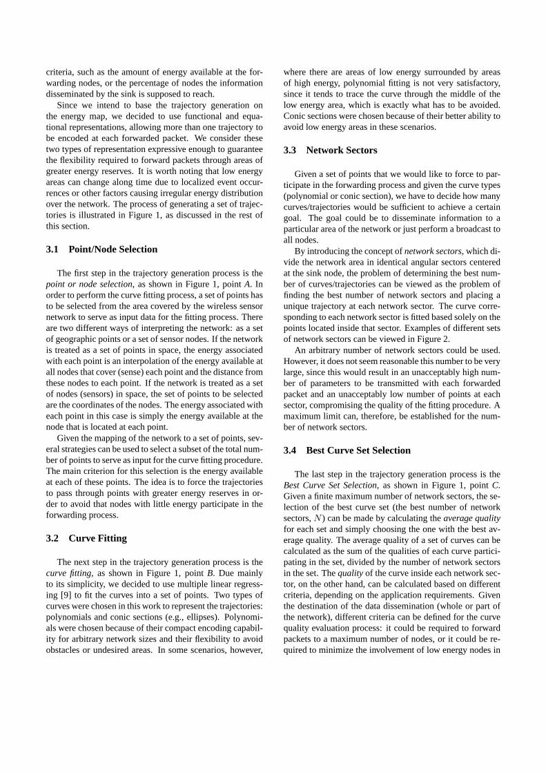
By introducing the concept ofnetwork sectors, which di-vide the network area in identical angular sectors centeredat the sink node, the problem of determining the best num-ber of curves/trajectories can be viewed as the problem offinding the best number of network sectors and placing aunique trajectory at each network sector. The curve corre-sponding to each network sector is fitted based solely on thepoints located inside that sector. Examples of different setsof network sectors can be viewed in Figure 2.

An arbitrary number of network sectors could be used.However, it does not seem reasonable this number to be verylarge, since this would result in an unacceptably high num-ber of parameters to be transmitted with each forwardedpacket and an unacceptably low number of points at eachsector, compromising the quality of the fitting procedure. Amaximum limit can, therefore, be established for the num-ber of network sectors.

3.4 Best Curve Set Selection

The last step in the trajectory generation process is theBest Curve Set Selection, as shown in Figure 1, pointC.Given a finite maximum number of network sectors, the se-lection of the best curve set (the best number of networksectors,N ) can be made by calculating theaverage qualityfor each set and simply choosing the one with the best av-erage quality. The average quality of a set of curves can becalculated as the sum of the qualities of each curve partici-pating in the set, divided by the number of network sectorsin the set. Thequalityof the curve inside each network sec-tor, on the other hand, can be calculated based on differentcriteria, depending on the application requirements. Giventhe destination of the data dissemination (whole or part ofthe network), different criteria can be defined for the curvequality evaluation process: it could be required to forwardpackets to a maximum number of nodes, or it could be re-quired to minimize the involvement of low energy nodes in

POINT/NODESELECTION FOR ANETWORK SECTOR

CURVE FITTINGFOR A

NETWORK SECTOR

BEST CURVE SET

SELECTION

EnergyMap

Set ofPoints

AllSets ofCurves

CurveEquations

Fit EvaluationCriterion

Destinationof the Data

Dissamination

NA B C

Figure 1. Trajectory generation process.

the forwarding process. Throughout this work, the follow-ing fit evaluation criteriawere used:

• Maximum average energy: calculates the aver-age energy of the nodes within the coveringrange of the curve (distance(node, curve) ≤node sensing range);

• Maximum coverage: calculates the total number ofnodes within the covering range of the curve.

In Figure 2, several snapshots of generated curve setsare shown for a given energy map. Figures 2-a through 2-cshow the sets of conic sections generated for that scenario.It can be observed that the trajectories avoid the low energyareas. Ifmaximum average energyor maximum coveragecriteria are used to select one of these sets of curves, thebest set is the one with four sectors. This result is obtainedsince theaverage qualityof the four participating curves inthis set was the best using both fit evaluation criteria. Fig-ures 2-d through 2-f show sets of fourth-degree polynomialsgenerated for the same network scenario. It can be observedthat once again most of the trajectories avoid the low energyareas. Ifmaximum average energycriterion is used to selectone of these sets of curves, the set of trajectories using onenetwork sector is chosen. This result is obtained becausethe average energy of the nodes within the covering rangeof this curve was lower than the average energy of the restof the curve sets. Ifmaximum coveragecriterion is used, onthe other hand, the best set is the one that uses eight sec-tors. This behavior is natural, since the greater the numberof curves, the greater the amount of nodes within their cov-ering range.

3.5 Some Remarks

It is important to point out that the trajectory generationstrategy proposed here is not restricted to the network sce-nario illustrated in Figure 2. An energy map of a networkwith an arbitrary shape and an arbitrary number of randomlydistributed sink nodes can be used as input to this procedure.In this situation, each node would be able to participate inmore than one trajectory, possibly forwarding packets orig-inated by different sink nodes.

Another relevant consideration is about the process ofencoding the trajectories. Curve parameters can be embed-ded in the packet header or can be pre-configured in thenodes before delivering them. However, in the latter, thesink node should be able to update those values periodically.

4 Data Dissemination

This section describes the TBF technique and introducesthe second part of our solution, which consists of a newforwarding policy mechanism, called TBF+.

4.1 Basic Operation of TBF

TBF is a data dissemination algorithm that uses curveequations to route messages. The trajectory is embeddedin each packet and the intermediate nodes make the for-warding decisions based on the trajectory and a neighbor ta-ble. To update the neighbor tables, nodes exchange beaconpackets periodically. The innovation of this approach comesfrom the definition and treatment of route paths as a contin-uous function as opposed to a discrete set of points. Twomain advantages of TBF are compact representation, sincecurves can be described using few parameters, and node in-dependence, since no particular node address is specified inthe trajectory.

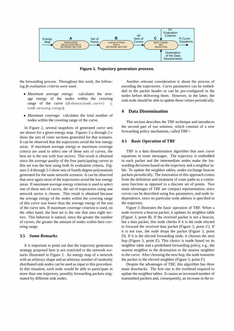
Figure 3 illustrates the basic operation of TBF. When anode receives a beacon packet, it updates its neighbor table(Figure 3, pointB). If the received packet is not a beacon,but a data packet, this node checks if it is the node electedto forward the received data packet (Figure 3, pointC). Ifit is not true, the node drops the packet (Figure 3, pointD). If it is the elected forwarding node, it chooses the nexthop (Figure 3, pointE). This choice is made based on itsneighbor table and a predefined forwarding policy, e.g., thenearest neighbor to the destination or the nearest neighborto the curve. After choosing the next hop, the node transmitsthe packet to the elected neighbor (Figure 3, pointF).

Despite the advantages of TBF, this algorithm has threemain drawbacks. The first one is the overhead required toupdate the neighbor tables. It causes an increased number oftransmitted packets and, consequently, an increase in the to-

(a) Curve set with one networksector.

(b) Curve set with two networksectors.

(c) Curve set with four net-work sectors.

(d) Curve set with one networksector.

(e) Curve set with five networksectors.

(f) Curve set with eight net-work sectors.

Figure 2. Conic sections and fourth degree polynomial trajectories traced upon the energy map.

DATA ORBEACON?

UPDATENEIGHBOR TABLE DROP

AM I THECHOSEN NODE?

CHOOSE THE NEXT NODE

FORWARDPACKET

ReceivedPacket

DataPacket Yes Next

Hop

NoBeacon

A

B

C

D

E F

Figure 3. Basic Operation of TBF.

INSIDENETWORK SECTOR?

EVALUATEDISTANCE

FROM CURVE

CALCULATEDISSAMINATION

DELAY TIMEWAIT

FORWARDPACKET

RECEIVED THE SAME

PACKET AGAIN?DROP

ReceivedPacket Yes Continue

DissaminationDelay Time

DissaminationDelay Time

No NoYes

TimeoutDrop

Packet

A

B

C D E

F G

Figure 4. Basic Operation of TBF +.

tal energy spent. The second disadvantage is its weak faulttolerance. This is due to the fact that the next node in aroute is determined based on the neighbor table of the pre-viously elected node. Since the decision of forwarding apacket is not made by the node itself, it can be in sleepingmode at the moment when the packet is transmitted to it.The more outdated the node table is, the higher the proba-bility of this problem to appear. The last weakness is dueto the fact that each packet embeds exactly one curve, sincepackets are relayed in a unicast manner. Therefore, a nodecan select only one neighbor to continue the process and,consequently, only one curve, which may not be sufficientto perform data dissemination to a significant part of thenetwork.

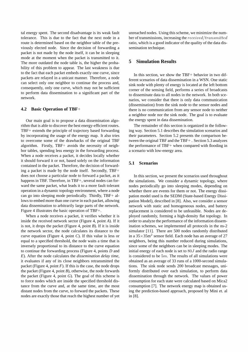
4.2 Basic Operation of TBF+

Our main goal is to propose a data dissemination algo-rithm that is able to discover the best energy-efficient routes.TBF+ extends the principle of trajectory based forwardingby incorporating the usage of the energy map. It also triesto overcome some of the drawbacks of the original TBFalgorithm. Firstly, TBF+ avoids the necessity of neigh-bor tables, spending less energy in the forwarding process.When a node receives a packet, it decides locally whetherit should forward it or not, based solely on the informationcontained in the packet. Therefore, the decision of forward-ing a packet is made by the node itself. Secondly, TBF+

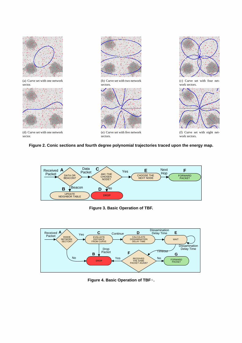
does not choose a particular node to forward a packet, as ithappens in TBF. Therefore, in TBF+, several nodes can for-ward the same packet, what leads it to a more fault tolerantoperation in a dynamic topology environment, where a nodecan go into sleeping mode periodically. Thirdly, TBF+ al-lows to embed more than one curve in each packet, allowingdata dissemination to arbitrarily large parts of the network.Figure 4 illustrates the basic operation of TBF+.

When a node receives a packet, it verifies whether it isinside the received network sector (Figure 4, pointA). If itis not, it drops the packet (Figure 4, pointB). If it is insidethe network sector, the node calculates its distance to thecurve equation (Figure 4, pointC). If this value is less orequal to a specified threshold, the node waits a time that isinversely proportional to its distance to the curve equationto continue the forwarding process (Figure 4, pointsD andE). After the node calculates thedissemination delay time,it evaluates if any of its close neighbors retransmitted thepacket (Figure 4, pointF). If this is the case, the node dropsthe packet (Figure 4, pointB), otherwise, the node forwardsthe packet (Figure 4, pointG). The goal of this scheme isto force nodes which are inside the specified threshold dis-tance from the curve and, at the same time, are the mostdistant nodes from the curve, to forward the packets. Thesenodes are exactly those that reach the highest number of yet

unreached nodes. Using this scheme, we minimize the num-ber of transmissions, increasing thereceived/transmittedratio, which is a good indicator of the quality of the data dis-semination technique.

5 Simulation Results

In this section, we show the TBF+ behavior in two dif-ferent scenarios of data dissemination in a WSN. One staticsink node with plenty of energy is located at the left bottomcorner of the sensing field, performs a series of broadcaststo disseminate data to all nodes in the network. In both sce-narios, we consider that there is only data communication(dissemination) from the sink node to the sensor nodes andthere is no communication from any sensor node to neithera neighbor node nor the sink node. The goal is to evaluatethe energy spent in data dissemination.

The remainder of this section is organized in the follow-ing way. Section 5.1 describes the simulation scenarios andtheir parameters. Section 5.2 presents the comparison be-tween the original TBF and the TBF+ . Section 5.3 analyzesthe performance of TBF+ when compared with flooding ina scenario with low-energy area.

5.1 Scenarios

In this section, we present the scenarios used throughoutthe simulations. We consider a dynamic topology, wherenodes periodically go into sleeping modes, depending onwhether there are events for them or not. The energy dissi-pation model used is the SEDM (State-based Energy Dissi-pation Model), described in [8]. Also, we consider a sensornetwork with static and homogeneous nodes, and batteryreplacement is considered to be unfeasible. Nodes are de-ployed randomly, forming a high-density flat topology. Inorder to analyze the performance of the information dissem-ination schemes, we implemented all protocols in the ns-2simulator [11]. There are 500 nodes randomly distributedin a 35×35m2 sensor field. Each node has an average of 27neighbors, being this number reduced during simulations,since some of the neighbors can be in sleeping modes. Theinitial energy of each node is set to80J and the radio rangeis considered to be5m. The results of all simulations wereobtained as an average of 33 runs of a 1000-second simula-tions. The sink node sends 200 broadcast messages, uni-formly distributed over each simulation, to perform datadissemination through the network. The values of powerconsumption for each state were calculated based on Mica2consumption [7]. The network energy map is obtained us-ing the prediction-based approach, proposed by Mini et. alin [8].

(a) TBF, time = 0s: coverage =86%, energy = 100%.

(b) TBF, time = 500s: cover-age = 40.7%, energy = 64.83%.

(c) TBF, time = 1000s: cover-age = 0%, energy = 31%.

(d) TBF+, time = 0s: coverage= 100%, energy = 100%.

(e) TBF+, time = 500s: cover-age = 54%, energy = 73.23%.

(f) TBF+, time = 1000s: cov-erage = 54%, energy = 46.5%.

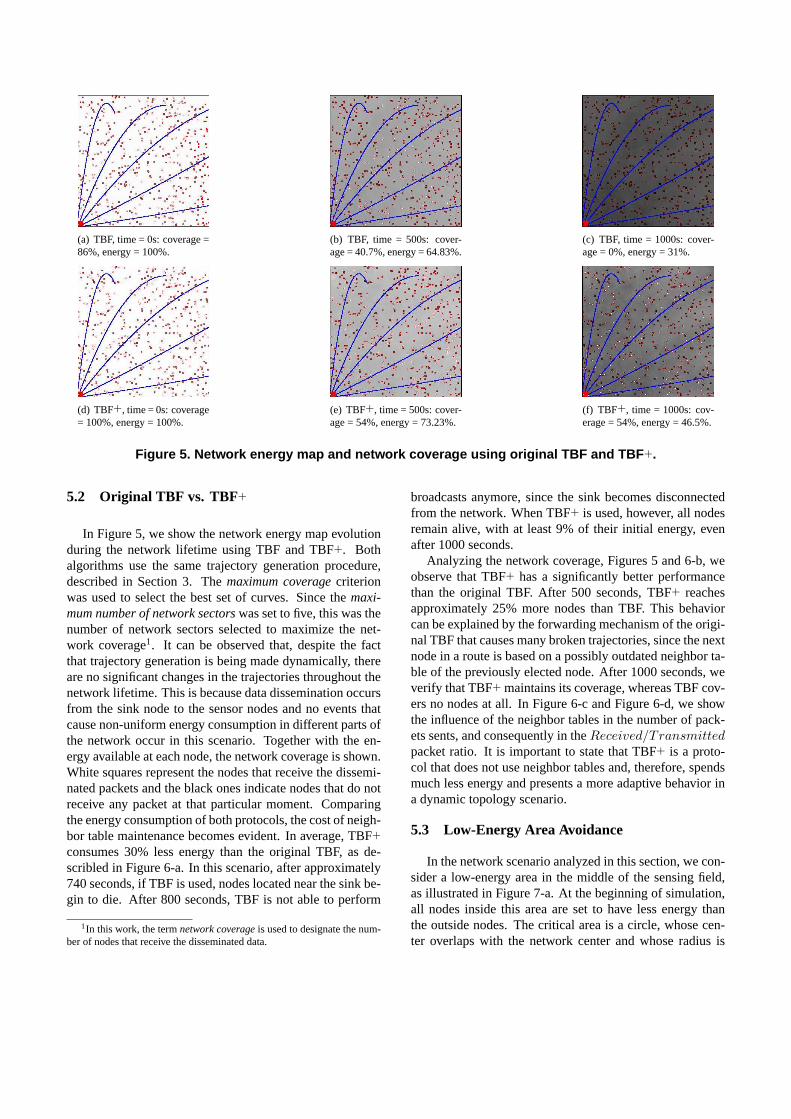
Figure 5. Network energy map and network coverage using original TBF and TBF +.

5.2 Original TBF vs. TBF+

In Figure 5, we show the network energy map evolutionduring the network lifetime using TBF and TBF+. Bothalgorithms use the same trajectory generation procedure,described in Section 3. Themaximum coveragecriterionwas used to select the best set of curves. Since themaxi-mum number of network sectorswas set to five, this was thenumber of network sectors selected to maximize the net-work coverage1. It can be observed that, despite the factthat trajectory generation is being made dynamically, thereare no significant changes in the trajectories throughout thenetwork lifetime. This is because data dissemination occursfrom the sink node to the sensor nodes and no events thatcause non-uniform energy consumption in different parts ofthe network occur in this scenario. Together with the en-ergy available at each node, the network coverage is shown.White squares represent the nodes that receive the dissemi-nated packets and the black ones indicate nodes that do notreceive any packet at that particular moment. Comparingthe energy consumption of both protocols, the cost of neigh-bor table maintenance becomes evident. In average, TBF+

consumes 30% less energy than the original TBF, as de-scribled in Figure 6-a. In this scenario, after approximately740 seconds, if TBF is used, nodes located near the sink be-gin to die. After 800 seconds, TBF is not able to perform

1In this work, the termnetwork coverageis used to designate the num-ber of nodes that receive the disseminated data.

broadcasts anymore, since the sink becomes disconnectedfrom the network. When TBF+ is used, however, all nodesremain alive, with at least 9% of their initial energy, evenafter 1000 seconds.

Analyzing the network coverage, Figures 5 and 6-b, weobserve that TBF+ has a significantly better performancethan the original TBF. After 500 seconds, TBF+ reachesapproximately 25% more nodes than TBF. This behaviorcan be explained by the forwarding mechanism of the origi-nal TBF that causes many broken trajectories, since the nextnode in a route is based on a possibly outdated neighbor ta-ble of the previously elected node. After 1000 seconds, weverify that TBF+ maintains its coverage, whereas TBF cov-ers no nodes at all. In Figure 6-c and Figure 6-d, we showthe influence of the neighbor tables in the number of pack-ets sents, and consequently in theReceived/Transmittedpacket ratio. It is important to state that TBF+ is a proto-col that does not use neighbor tables and, therefore, spendsmuch less energy and presents a more adaptive behavior ina dynamic topology scenario.

5.3 Low-Energy Area Avoidance

In the network scenario analyzed in this section, we con-sider a low-energy area in the middle of the sensing field,as illustrated in Figure 7-a. At the beginning of simulation,all nodes inside this area are set to have less energy thanthe outside nodes. The critical area is a circle, whose cen-ter overlaps with the network center and whose radius is

0

20

40

60

80

100

0 100 200 300 400 500 600 700 800 900 1000

Mea

n E

nerg

y (%

)

Time (s)

TBF+TBF

(a) Mean Energy.

0

20

40

60

80

100

0 100 200 300 400 500 600 700 800 900 1000

Rea

ched

Nod

es p

er b

road

cast

(%

)

Time (s)

TBF+TBF

(b) Reached nodes.

0

20000

40000

60000

80000

100000

120000

140000

0 100 200 300 400 500 600 700 800 900 1000

Num

ber

of T

rans

mitt

ed P

acke

ts

Time (s)

TBF+TBF

(c) Packets transmitted.

0

0.5

1

1.5

2

2.5

3

3.5

4

4.5

0 100 200 300 400 500 600 700 800 900 1000

Rec

eive

d / T

rans

mitt

ed R

atio

Time (s)

TBF+TBF

(d) Received/Transmitted ratio.

Figure 6. Results for the Original TBF and the TBF + .

equals to 7 m. The number of nodes randomly deployedinside the critical region is 53. The comparisons are madewith flooding and gossiping-based approaches with proba-bility. The maximum average energy criterion, described inSection 3.4, is used to generate the trajectories for TBF+.It can be observed that the generated trajectories avoid thelow-energy area (Figure 8-a), however, once again no sig-nificant changes occur in their shapes along time. This iscaused by the fact that the relation between the averageenergy of the nodes located inside the low-energy and thehigh-energy areas is maintained. In the beginning of thenetwork lifetime, (Figure 7-a and 7-c), it can be seen thatflooding covers 100% of the nodes located inside the lowenergy area, whereas TBF+, due to its trajectory generationfeature, reaches only 31.4% of the low-energy nodes (Fig-ure 8-b). The cost of this difference can be seen after 500seconds (Figure 7-b and 7-e). Flooding kills the majority ofnodes inside the low-energy area (Figure 8-c), achieving anetwork coverage approximately 25% lower than TBF+ in-side this area. The average energy of these nodes decreasesapproximately 60% when TBF+ is used and 100% whenflooding is used (Figure 8-d). Outside the low-energy area,however, flooding still maintains a significantly better net-work coverage.

The cost of this high coverage can be seen in the nexttime snapshot (Figure 7-c and 7-f). After 1000 seconds,when flooding is used, the average energy of nodes locatedoutside the low-energy area is nearly 10% and the networkis completely disconnected, whereas when TBF+ is used,the average energy remains above above 35% and the net-work coverage is approximately 30% of the network.

It can be concluded that avoiding packet transmission bynodes with little energy, it is possible to prolong the life-time of these nodes, still guaranteeing that they receive thedata disseminated by the sink node. Despite providing abetter network coverage, flooding-based data disseminationimposes extremely high costs in terms of energy consump-tion. This fact compromises, firstly, the low-energy nodesand, eventually, the network lifetime as a whole.

6 Analytical Model

In this section, we propose an analytical model to val-idate the simulation results for TBF+ . Given a networkconfiguration (node locations) and a set of curves, the goalis to obtain the upper and the lower bounds of the expectednetwork coverage. Moreover, this model determines if thereis a possibility of broken trajectory occurrence during theforwarding process. This happens when there are no nodeswithin a specified threshold.

The upper bound of network coverage is computed as-suming that all nodes have their radios on, and, thus, all ofthem are able to receive and relay packets. The upper boundfor the number of nodes that receive a certain broadcast is,therefore, equal to the number of nodes within the specifiedthreshold distance from the curves, plus all nodes within theradio range distance from them.

To calculate the lower bound, we would have to assumethat all nodes have their radios off. However, since it is atrivial scenario, we defined the lower bound as the worstreceived/transmitted packet ratio. It means that, in theworst case, only the transmitting nodes would receive thebroadcasted data. The lower bound is, therefore, equal tothe number of nodes that decide to transmit the dissemi-nated information according to the three criteria presentedin Section 4.

We also analyze the broken trajectory occurrence. Tothis end, we defined a probabilityP of a node within the∆-curve to be with its radio off. We also defined a desiredrate of reliabilityR, that represents the number of neighborsthat a node has to have for the forwarding process to be con-tinued. In this case, the node must have at leastn neighborswithin the∆-curve at a more advanced point on the trajec-tory (backward nodes are not considered). The value ofncan be calculated if the probability of at least one neighborbeing awake is higher or equals the reliability rate. This isrepresented by the equations below:

(1− Pn) ≥ RPn ≤ 1−R

n ≥ logP (1−R)n = dlogP (1−R)e

(1)

(a) Flooding, time = 0s: Ci =100%, Ei = 33%, Co = 100%,Eo = 100%.

(b) Flooding, time = 500s: Ci= 9.4%, Ei = 0,2%, Co =79,2%, Eo = 59.4%.

(c) Flooding, time = 1000s: Ci= 0%, Ei = 0%, Co = 0%, Eo =9.4%.

(d) TBF+, time = 0s: Ci =31.4%, Ei = 33%, Co = 84.1%,Eo = 100%.

(e) TBF+, time = 500s: Ci =12.3%, Ei = 12,1%, Co = 35%,Eo = 75.4%.

(f) TBF+, time = 1000s: Ci =0%, Ei = 0%, Co = 35%, Eo =41%.

Legend: Ci/Co = Coverage inside/outside the low-energy areaEi/Eo = Energy inside/outside the low-energy area

Figure 7. Network energy map and network coverage using flooding and TBF + in a low-energy-areascenario.

0

500

1000

1500

2000

2500

3000

3500

0 100 200 300 400 500 600 700 800 900 1000

Num

ber

of T

rans

mitt

ed P

acke

ts

Time (s)

TBF+Flooding

(a) Number of transmitted packets.

0

20

40

60

80

100

0 100 200 300 400 500 600 700 800 900 1000

Rea

ched

Nod

es p

er b

road

cast

(%

)

Time (s)

TBF+Flooding

(b) Reached nodes.

0

20

40

60

80

100

0 100 200 300 400 500 600 700 800 900 1000

Dea

d N

ode

(%)

Time (s)

TBF+Flooding

(c) Number of dead nodes.

0

20

40

60

80

100

0 100 200 300 400 500 600 700 800 900 1000

Mea

n E

nerg

y (%

)

Time (s)

TBF+Flooding

(d) Mean energy.

Figure 8. Results for nodes inside the low-energy area

Figure 9. A snapshot ofthe network for the upperbound scenario.

Figure 10. A snapshot ofthe network for the lowerbound scenario.

Figure 11. An example of abroken trajectory.

In Table 1, we show the network covering bounds for theset of curves illustrated in Figures 9, 10 and 11. This set ofcurves was selected by the trajectory definition algorithm,presented in Section 3, and was used during one of the per-formed simulations. In all of these figures, we consider thenetwork scenario used in Section 5.3. It is worth noting thatthroughout the simulations, described in Section 5, TBF+

performance was near the upper bound. In Figure 9, weshow the upper bound coverage. In this case, the nodes thattransmit packets are in black, those that only receive pack-ets are in gray and the others are in light gray. In Figure 10,we show the same aspects for the lower bound scenario. Fi-nally, in Figure 11, we present an example of a broken tra-jectory. In this figure, we observe that the trajectory brakesonly in the upper network sector curve.

Table 1. The network covering for the upperand the lower bounds.

Case Reached Nodes

Upper Bound 77.8%Lower Bound 10.8%Simulation Result 63.51%

7 Conclusions and Future Work

In this paper, we propose TBF+, a new data dissemina-tion scheme for WSNs. The key idea is to combine conceptspresented in trajectory-based forwarding with the informa-tion provided by the energy map of the network. We pro-posed a method not only for representing the trajectories,but also for specifying them dynamically based on the en-ergy map, which changes along the network lifetime. Inthe original TBF, nodes use a forwarding technique basedon neighbor tables. This technique requires a high energyoverhead to be updated, and its mechanism is not suitablefor operating in dynamic topology models, where nodes canoften go into sleeping modes. TBF+ replaces this mecha-nism with a new forwarding technique: when a node re-ceives a packet, it decides by itself if it should forward thepacket based solely on its own location and the equationembedded in the packet. The simulations showed that ifTBF+ is used, the routing process becomes more adaptiveto changes in network topology. Moreover, the energy spentwith the routing activity can be concentrated on those nodesthat have high energy reserves, whereas low-energy nodescan be left to use their energy only to perform the sensingactivity or to receive information addressed to them.

There are several improvements that we are planning tointroduce to the curve generation procedure. One aspect to

be explored is the way of interpreting the network. Cur-rently, we are representing the network as a set of sensors,whose coordinates are used as input to the curve fitting pro-cedure. Another interesting manner of performing the map-ping is by viewing the network as a set of geographic points,whose energy reserves are calculated as an interpolation ofthe energy of those sensor nodes that cover each point. Inthis work, we established two criteria to select the best setof curves from all sets of curves generated using differentcurve types and different numbers of sectors. We plan topropose new selection criteria, possibly combining or alter-nating them in a dynamic fashion, depending on the applica-tion requirements. Another future work is to introduce othertechniques to avoid transmissions inside the low-energy re-gion. For example, we can use a energy threshold to al-low nodes that have less energy than a certain pre-definedamount to not forward data.

References

[1] I. F. Akyildiz, W. Su, Y. Sankarasubramaniam, andE. Cayirci. Wireless sensor networks: A survey.ComputerNetworks, 38(4):393–422, 2002.

[2] D. Estrin, R. Govindan, J. Heidemann, and S. Kumar. Nextcentury challenges: scalable coordination in sensor net-works. InMOBICOM 99, pages 263–270, USA, 1999.

[3] D. Ganesan, R. Govindan, S. Shenker, and D. Estrin.Highly-resilient, energy-efficient multipath routing in wire-less sensor networks.ACM Mobile Computing and Commu-nications Review, 5(4), October 2001.

[4] C. Intanagonwiwat, D. Estrin, R. Govindan, and J. Heide-mann. Directed diffusion: a scalable and robust communi-cation paradigm for sensor networks. InICDCS 02, Vienna,Austria, 2002.

[5] C. Intanagonwiwat, R. Govindan, and D. Estrin. Directeddiffusion: a scalable and robust communication paradigmfor sensor networks. InProceedings of the sixth annual in-ternational conference on Mobile computing and network-ing, pages 56–67, Boston, MA USA, 2000.

[6] J. M. Kahn, R. H. Katz, and K. S. J. Pister. Next centurychallenges: Mobile networking for smart dust. InIn Pro-ceedings of MOBICOM, pages 271–278, Seattle, 1999.

[7] Mica2. Mts/mda sensor and data acquisition boards user’smanual. www.xbow.com, 2004.

[8] R. A. F. Mini, M. do Val Machado, A. A. F. Loureiro, andB. Nath. Prediction-based energy map for wireless sensornetworks.Ad Hoc Networks Journal, 2004. To appear.

[9] D. C. Montgomery, E. A. Peck, and G. G. Vining.Intro-duction to Linear Regression Analysis. John Wiley & Sons,2001.

[10] D. Niculescu and B. Nath. Trajectory-Based Forwarding andits Applications. InMOBICOM 03, pages 260–272, USA,2003.

[11] ns2. The network simulator. www.isi.edu/nsnam/ns, 2002.