Data Augmentation with Variational Autoencoders and ...

HAL Id: hal-03180775https://hal.archives-ouvertes.fr/hal-03180775v2

Submitted on 21 Oct 2021

HAL is a multi-disciplinary open accessarchive for the deposit and dissemination of sci-entific research documents, whether they are pub-lished or not. The documents may come fromteaching and research institutions in France orabroad, or from public or private research centers.

L’archive ouverte pluridisciplinaire HAL, estdestinée au dépôt et à la diffusion de documentsscientifiques de niveau recherche, publiés ou non,émanant des établissements d’enseignement et derecherche français ou étrangers, des laboratoirespublics ou privés.

Data Augmentation with Variational Autoencoders andManifold Sampling

Clément Chadebec, Stéphanie Allassonnière

To cite this version:Clément Chadebec, Stéphanie Allassonnière. Data Augmentation with Variational Autoencoders andManifold Sampling. DALI 2021 : 1st MICCAI Workshop on Data Augmentation, Labeling, andImperfections, Oct 2021, Strasbourg, France. �hal-03180775v2�

Data Augmentation with VariationalAutoencoders and Manifold Sampling

Clement Chadebec and Stephanie Allassonniere

Universite de Paris, INRIA, Centre de recherche des Cordeliers, INSERM, SorbonneUniversite, Paris, France

{clement.chadebec, stephanie.allassonniere}@inria.fr

Abstract. We propose a new efficient way to sample from a VariationalAutoencoder in the challenging low sample size setting1. This methodreveals particularly well suited to perform data augmentation in such alow data regime and is validated across various standard and real-lifedata sets. In particular, this scheme allows to greatly improve classifica-tion results on the OASIS database where balanced accuracy jumps from80.7% for a classifier trained with the raw data to 88.6% when trainedonly with the synthetic data generated by our method. Such results werealso observed on 3 standard data sets and with other classifiers.

Keywords: Data Augmentation · VAE · Latent space modelling

1 Introduction

Despite the apparent availability of always bigger data sets, the lack of dataremains a key issue for many fields of application. One of them is medicinewhere practitioners have to deal with potentially very high dimensional data(e.g. functional Magnetic Resonance Imaging for neuroimaging) along with verylow sample sizes (e.g. rare diseases or heterogeneous cancers) which make statis-tical analysis challenging and unreliable. In addition, the wide use of algorithmsheavily relying on the deep learning framework [6] and requiring a large amountof data has made the need for data augmentation (DA) crucial to avoid poorperformance or over-fitting [19]. As an example, a classic way to perform DA onimages consists in applying simple transformations such as adding random noise,rotations etc. However, it may be easily understood that such augmentation tech-niques are strongly data dependent2 and may still require the intervention of anexpert assessing the relevance of the augmented samples. The recent develop-ment of generative models such as Generative Adversarial Networks (GAN) [7]or Variational AutoEncoders (VAE) [10,17] paves the way for consideration ofanother way to augment the training data. While GANs have already seen somesuccess [4,22,2] and even for medical data [13,18] VAEs have been of least inter-est. One limitation of the use of both generative models relies in their need of a

1 A code is available at https://github.com/clementchadebec/Data Augmentationwith VAE-DALI

2 Think of digits where rotating a 6 gives a 9 for example.

2 Chadebec and Allassonniere

large amount of data to be able to generate faithfully. In this paper, we arguethat VAEs can actually be used to perform DA in challenging contexts providedthat we amend the way we generate the data. Hence, we propose:

– A new non prior-dependent generation method using the learned geometryof the latent space and consisting in exploring it by sampling along geodesics.

– To use this method to perform DA in the small sample size setting on stan-dard data sets and real data from OASIS database [16] where it allows toremarkably improve classification results.

2 Variational Autoencoder

Given a set of data x ∈ X , a VAE aims at maximizing the likelihood of the asso-ciated parametric model {Pθ, θ ∈ Θ}. Assuming that there exist latent variablesz ∈ Z living in a lower dimensional space Z, the marginal distribution writes

pθ(x) =

∫Z

pθ(x|z)q(z)dz , (1)

where q is a prior distribution over the latent variables and pθ(x|z) is most ofthe time a simple distribution and is referred to as the decoder. A variationaldistribution qϕ (often taken as Gaussian) aiming at approximating the true pos-terior distribution and referred to as the encoder is then introduced. Using Im-portance Sampling allows to derive an unbiased estimate of pθ(x) such thatEz∼qϕ

[pθ]

= pθ(x). Therefore, a lower bound on the logarithm of the objectivefunction of Eq. (1) can be derived using Jensen’s inequality:

log pθ(x) ≥ Ez∼qϕ[

log pθ(x, z)− log qϕ(z|x)]

= ELBO . (2)

Using the reparametrization trick makes the ELBO tractable and so can beoptimised with respect to both θ and ϕ, the encoder and decoder parameters.Once the model is trained, the decoder acts as a generative model and new datacan be generated by simply drawing a sample using the prior q and feeding it tothe decoder. Several axes of improvement of this model were recently explored.One of them consists in trying to bring geometry into the model by learning thelatent structure of the data seen as a Riemannian manifold [3,5].

3 Some Elements on Riemannian Geometry

In the framework of differential geometry, one may define a Riemannian manifoldM as a smooth manifold endowed with a Riemannian metric G which is a smoothinner product G : p → 〈·|·〉p on the tangent space TpM defined at each pointp of the manifold. The length of a curve γ between two points of the manifoldz1, z2 ∈ M and parametrized by t ∈ [0, 1] such that γ(0) = z1 and γ(1) = z2 is

given by L(γ) =1∫0

‖γ(t)‖γ(t)dt =1∫0

√〈γ(t)|γ(t)〉γ(t)dt . Curves minimizing such

Data Augmentation with Variational Autoencoders and Manifold Sampling 3

a length are called geodesics. For any p ∈ M, the exponential map at p, Expp,maps a vector v of the tangent space TpM to a point of the manifold p ∈ Msuch that the geodesic starting at p with initial velocity v reaches p at time 1.In particular, if the manifold is geodesically complete, then Expp is defined onthe entire tangent space TpM.

4 The Proposed Method

We propose a new sampling method exploiting the structure of the latent spaceseen as a Riemannian manifold and independent from the choice of the priordistribution. The view we adopt is to consider the VAE as a tool to performdimensionality reduction by extracting the latent structure of the data within alower dimensional space. Having learned such a structure, we propose to exploit itto enhance the data generation process. This differs from the fully probabilisticview which uses the prior to generate. We believe that this is far from beingoptimal since the prior appears quite strongly data dependent. We will adoptthe same setting as [5] and so use a RHVAE since the metric used by the authorsis easily computable, constraints geodesic path to travel through most populatedareas of the latent space and the learned Riemannian manifold is geodesicallycomplete. Nonetheless, the proposed method can be used with different metricsas well as long as the exponential map remains computable. We now assumethat we are given a latent space with a Riemannian structure where the metrichas been estimated from the input data.

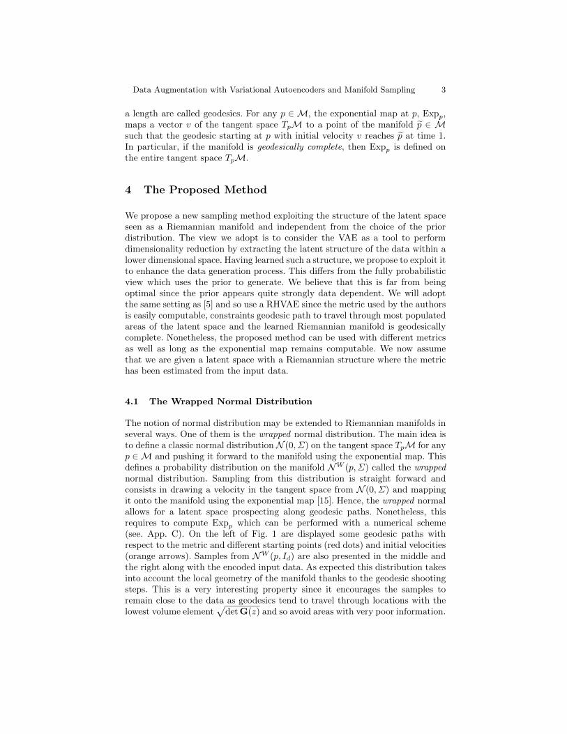
4.1 The Wrapped Normal Distribution

The notion of normal distribution may be extended to Riemannian manifolds inseveral ways. One of them is the wrapped normal distribution. The main idea isto define a classic normal distribution N (0, Σ) on the tangent space TpM for anyp ∈M and pushing it forward to the manifold using the exponential map. Thisdefines a probability distribution on the manifold NW (p,Σ) called the wrappednormal distribution. Sampling from this distribution is straight forward andconsists in drawing a velocity in the tangent space from N (0, Σ) and mappingit onto the manifold using the exponential map [15]. Hence, the wrapped normalallows for a latent space prospecting along geodesic paths. Nonetheless, thisrequires to compute Expp which can be performed with a numerical scheme(see. App. C). On the left of Fig. 1 are displayed some geodesic paths withrespect to the metric and different starting points (red dots) and initial velocities(orange arrows). Samples from NW (p, Id) are also presented in the middle andthe right along with the encoded input data. As expected this distribution takesinto account the local geometry of the manifold thanks to the geodesic shootingsteps. This is a very interesting property since it encourages the samples toremain close to the data as geodesics tend to travel through locations with thelowest volume element

√det G(z) and so avoid areas with very poor information.

4 Chadebec and Allassonniere

−10 −5 0 5 10

−10

−5

0

5

10geodesic

velocity

starting point

−0.5

0.0

0.5

1.0

1.5

2.0

2.5

3.0

−10 −5 0 5 10−10.0

−7.5

−5.0

−2.5

0.0

2.5

5.0

7.5

10.0

rings

circles

samples

−0.5

0.0

0.5

1.0

1.5

2.0

2.5

3.0

−10 −5 0 5 10−10.0

−7.5

−5.0

−2.5

0.0

2.5

5.0

7.5

10.0

rings

circles

samples

−0.5

0.0

0.5

1.0

1.5

2.0

2.5

3.0

Fig. 1: Left : Geodesic shooting in a latent space learned by a RHVAE with dif-ferent starting points (red dots) and initial velocities (orange arrows). Middleand right : Samples from the wrapped normal NW (p, Id). The log metric volumeelement log

√det G(z) is presented in gray scale.

4.2 Riemannian Random Walk

A natural way to explore the latent space of a VAE consists in using a randomwalk like algorithm which moves from one location to another with a certainprobability. The idea here is to create a geometry-aware Markov Chain (zt)t∈Nwhere zt+1 is sampled using the wrapped normal zt+1 ∼ NW (zt, Σ). However,a drawback of such a method is that every sample of the chain is acceptedregardless of its relevance. Nonetheless, by design, the learned metric is suchthat it has a high volume element far from the data [5]. This implies that itencodes in a way the amount of information contained at a specific location ofthe latent space. The higher the volume element, the less information we have.The same idea was used in [11] where the author proposed to see the inversemetric volume element as a maximum likelihood objective to perform metriclearning. In our case the likelihood definition writes

L(z) =ρS(z)

√det G−1(z)∫

RdρS(z)

√det G−1(z)dz

, (3)

where ρS(z) = 1 if z ∈ S, 0 otherwise, and S is taken as a compact set so thatthe integral is well defined. Hence, we propose to use this measure to assess thesamples quality as an acceptance-rejection rate α in the chain where α(z, z) =

min

(1,

√detG−1(z)√detG−1(z)

), z is the current state of the chain and z is the proposal

obtained by sampling from the wrapped Gaussian NW (z,Σ). The idea is tocompare the relevance of the proposed sample to the current one. The ratio issuch that any new sample improving the likelihood metric L is automaticallyaccepted while a sample degrading the measure is more likely to be rejected inthe spirit of Hasting-Metropolis sampler. A pseudo-code is provided in Alg. 1.

Data Augmentation with Variational Autoencoders and Manifold Sampling 5

Algorithm 1 Riemannian random walk

Input: z0, Σfor t = 1→ T do

Draw vt ∼ N (0, Σ)zt ← Expzt−1

(vt)Accept the proposal zt with probability α

end for

4.3 Discussion

It may be easily understood that the choice of the covariance matrix Σ in Alg. 1has quite an influence on the resulting sampling. On the one hand, a Σ withstrong eigenvalues will imply drawing velocities of potentially high magnitudeallowing for a better prospecting but proposals are more likely to be rejected.On the other hand, small eigenvalues involve a high acceptance rate but it willtake longer to prospect the manifold. An adaptive method where Σ depends onG may be considered and will be part of future work.

Remark 1 If Σ has small enough eigenvalues then Alg. 1 samples from Eq. (3)

For the following DA experiments we will assume that Σ has small eigenvaluesand so will sample directly using this distribution. See app. A for sampling resultsusing the aforementioned method.

5 Data Augmentation Experiments For Classification

In this section, we explore the ability of the method to enrich data sets to improveclassification results.

5.1 Augmentation Setting

We first test the augmentation method on three reduced data sets extractedfrom well-known databases MNIST and EMNIST. For MNIST, we select 500samples applying either a balanced split or a random split ensuring that someclasses are far more represented. For EMNIST, we select 500 samples from 10classes such that they are composed of both lowercase and uppercase charactersso that we end up with a small database with strong variability within classes.These data sets are then split such that 80% is allocated for training (referredto as the raw data) and 20% for validation. For a fair comparison, we use theoriginal test set (e.g. ∼1000 samples per class for MNIST) to test the classifiers.This ensures statistically meaningful results while assessing the generalisationpower on unseen data. We also validate the proposed DA method on the OASISdatabase which represents a nice example of day-to-day challenges practitionershave to face and is a benchmark database. We use 2D gray scale MR Images(208x176) with a mask notifying brain tissues and are referred to as the masked

6 Chadebec and Allassonniere

Table 1: Summary of OASIS database demographics, mini-mental state exami-nation (MMSE) and global clinical dementia rating (CDR) scores.

Data set Label Obs. Age Sex M/F MMSE CDR

OASISCN 316 45.1± 23.9 119/197 29.1± 1.1 0: 316AD 100 76.8± 7.1 41/59 24.3± 4.1 0.5: 70 , 1: 28, 2: 2

TrainCN 220 45.6± 23.6 86/134 29.1± 1.2 0: 220AD 70 77.4± 6.8 29/41 23.7± 4.3 0.5: 47 , 1: 21, 2: 2

ValCN 30 48.9± 24.1 11/19 29.2± 0.8 0: 30AD 12 75.4± 7.2 4/8 25.8± 4.2 0.5: 7 , 1: 5, 2: 0

TestCN 66 41.7± 24.3 22/44 29.0± 1.0 0: 66AD 18 75.1± 7.5 8/10 25.8± 2.7 0.5: 16 , 1: 2, 2: 0

T88 images in [16]. We refer the reader to their paper for further image pre-processing details. We consider the binary classification problem consisting intrying to detect MRI of patients having been diagnosed with Alzheimer Disease(AD). We split the 416 images into a training set (70%) (raw data), a valida-tion set (10%) and a test set (20%). A summary of demographics, mini-mentalstate examination (MMSE) and global clinical dementia rating (CDR) is madeavailable in Table. 1. On the one hand, for each data set, the train set (rawdata) is augmented by a factor 5, 10 and 15 using classic DA methods (randomnoise, cropping etc.). On the other hand, VAE models are trained individuallyon each class of the raw data. The generative models are then used to produce200, 500, 1k or 2k synthetic samples per class with either the classic generationscheme (i.e. the prior) or the proposed method. We then train classifiers with 5independent runs on 1) the raw data; 2) the augmented data using basic trans-formations; 3) the augmented data using the VAE models; 4) only the syntheticdata generated by the VAEs. A DenseNet model3 [8] is used for the toy datawhile we also train hand made MLP and CNN models on OASIS (See App. E).The main metrics obtained on the test set are reported in Tables. 2 and 3.

5.2 Results

Toy Data As expected generating new samples using the proposed methodimproves their relevance. The method indeed allows for a quite impressive gain inthe model accuracy when synthetic samples are added to the real ones (leftmostcolumn of Table. 2). This is even more striking when looking at the rightmostcolumn where only synthetic samples are used to train the classifier. For instance,when only 200 synthetic samples per class for MNIST are generated with a VAEand used to train the classifier, the classic method fails to produce meaningfulsamples since a loss of 20 pts in accuracy is observed when compared to theraw data. Interestingly, our method seems to avoid such an effect. Even more

3 We use the code in [1] (See App. E).

Data Augmentation with Variational Autoencoders and Manifold Sampling 7

Table 2: DA on toy data sets. Mean accuracy and standard deviation across 5independent runs are reported. In gray are the cells where the accuracy is higheron synthetic data than on the raw data.

Data sets MNIST MNIST** EMNIST** MNIST MNIST** EMNIST**

Raw data 89.9 (0.6) 81.6 (0.7) 82.6 (1.4) - - -

Raw + Synthetic Synthetic only

Aug. (X5) 92.8 (0.4) 86.5 (0.9) 85.6 (1.3) - - -Aug. (X10) 88.3 (2.2) 82.0 (2.4) 85.8 (0.3) - - -Aug. (X15) 92.8 (0.7) 85.9 (3.4) 86.6 (0.8) - - -

VAE-200* 88.5 (0.9) 84.1 (2.0) 81.7 (3.0) 69.9 (1.5) 64.6 (1.8) 65.7 (2.6)VAE-500* 90.4 (1.4) 87.3 (1.2) 83.4 (1.6) 72.3 (4.2) 69.4 (4.1) 67.3 (2.4)VAE-1k* 91.2 (1.0) 86.0 (2.5) 84.4 (1.6) 83.4 (2.4) 74.7 (3.2) 75.3 (1.4)VAE-2k* 92.2 (1.6) 88.0 (2.2) 86.0 (0.2) 86.6 (2.2) 79.6 (3.8) 78.9 (3.0)

RHVAE-200* 89.9 (0.5) 82.3 (0.9) 83.0 (1.3) 76.0 (1.8) 61.5 (2.9) 59.8 (2.6)RHVAE-500* 90.9 (1.1) 84.0 (3.2) 84.4 (1.2) 80.0 (2.2) 66.8 (3.3) 67.0 (4.0)RHVAE-1k* 91.7 (0.8) 84.7 (1.8) 84.7 (2.4) 82.0 (2.9) 69.3 (1.8) 73.7 (4.1)RHVAE-2k* 92.7 (1.4) 86.8 (1.0) 84.9 (2.1) 85.2 (3.9) 77.3 (3.2) 68.6 (2.3)

Ours-200* 91.0 (1.1) 84.1 (2.0) 85.1 (1.1) 87.2 (1.1) 79.5 (1.6) 77.1 (1.6)Ours-500* 92.3 (1.1) 87.7 (0.9) 85.1 (1.1) 89.1 (1.3) 80.4 (2.1) 80.2 (2.0)Ours-1k* 93.3 (0.8) 89.7 (0.8) 87.0 (1.0) 90.2 (1.4) 86.2 (1.8) 82.6 (1.3)Ours-2k* 94.3 (0.8) 89.1 (1.9) 87.6 (0.8) 92.6 (1.1) 87.6 (1.3) 86.0 (1.0)

* Number of generated samples ** Unbalanced data sets

impressive is the fact that we are able to produce synthetic data sets on whichthe classifier outperforms greatly the results observed on the raw data (3 to 6pts gain in accuracy) while keeping a relatively low standard deviation (see graycells). Secondly, this example also shows why geometric DA is still questionableand remains data dependent. For instance, augmenting the raw data by a factor10 (including flips and rotations) does not seem to have a notable effect on theMNIST data sets but still improves results on EMNIST. On the contrary, ourmethod seems quite robust to data set changes.

OASIS Balanced accuracy obtained on OASIS with 3 classifiers is made avail-able in Table. 3. In this experiment, using the new generation scheme againimproves overall the metric for each classifier when compared to the raw dataand other augmentation methods. Moreover, the strong relevance of the cre-ated samples is again supported by the fact that the classifiers are again ableto strongly outperform the results on the raw data even when trained only withsynthetic ones. Finally, the method appears robust to classifiers and can beused with high-dimensional complex data such as MRI.

6 Conclusion

In this paper, we proposed a new way to generate new data from a VariationalAutoencoder which has learned the latent geometry of the input data. Thismethod was then used to perform DA to improve classification tasks in the low

8 Chadebec and Allassonniere

Table 3: DA on OASIS data base. Mean balanced accuracy on independent 5runs with several classifiers.

Networks MLP CNN Densenet

Raw data 80.7 (4.1) - 72.5 (3.5) - 77.4 (3.3) -

Raw + Synthetic Raw + Synthetic Raw + SyntheticSynthetic Only Synthetic Only Synthetic Only

Aug. (X5) 84.3 (1.3) - 80.0 (3.5) - 73.9 (5.1) -Aug. (X10) 76.0 (2.8) - 82.8 (3.7) - 78.3 (4.1) -Aug. (X15) 78.7 (5.3) - 80.3 (3.7) - 76.6 (1.1) -

VAE-200∗ 80.7 (1.5) 77.8 (1.3) 79.4 (3.6) 65.0 (12.3) 76.5 (3.2) 74.0 (3.0)VAE-500∗ 79.7 (1.4) 77.4 (1.5) 72.6 (7.0) 70.2 (5.0) 74.9 (4.3) 72.8 (1.8)VAE-1000∗ 81.3 (0.0) 76.5 (0.6) 74.4 (9.4) 73.0 (3.3) 73.5 (1.3) 74.9 (2.6)VAE-2000∗ 80.7 (0.3) 78.1 (1.6) 71.1 (4.9) 76.9 (2.6) 74.0 (4.9) 73.3 (3.4)

Ours-200∗ 84.3 (0.0) 86.7 (0.4) 76.4 (5.0) 75.4 (6.6) 78.2 (3.0) 74.3 (4.8)Ours-500∗ 87.2 (1.2) 88.6 (1.1) 81.8 (4.6) 81.8 (3.7) 80.2 (2.8) 84.2 (2.8)Ours-1000∗ 84.2 (0.3) 84.4 (1.8) 83.5 (3.2) 79.8 (2.8) 82.2 (4.7) 76.7 (3.8)Ours-2000∗ 85.3 (1.9) 84.2 (3.3) 84.5 (1.9) 83.9 (1.9) 82.9 (1.8) 73.6 (5.8)

* Number of generated samples

sample size setting on both toy and real data and with different kind of classi-fiers. In each case, the method allows for an impressive gain in the classificationmetrics (e.g. balanced accuracy jumps from 80.7 to 88.6 on OASIS). Moreover,the relevance of the generated data was supported by the fact that classifierswere able to perform better when trained with only synthetic data than on theraw data in all cases. Future work would consist in using the method on evenmore challenging data such as 3D volumes and using smaller data sets.

Acknowledgment

The research leading to these results has received funding from the French gov-ernment under management of Agence Nationale de la Recherche as part of the“Investissements d’avenir” program, reference ANR-19-P3IA-0001 (PRAIRIE3IA Institute) and reference ANR-10-IAIHU-06 (Agence Nationale de la Recher-che-10-IA Institut Hospitalo-Universitaire-6). Data were provided in part by OA-SIS: Cross-Sectional: Principal Investigators: D. Marcus, R, Buckner, J, Cser-nansky J. Morris; P50 AG05681, P01 AG03991, P01 AG026276, R01 AG021910,P20 MH071616, U24 RR021382

Data Augmentation with Variational Autoencoders and Manifold Sampling 9

References

1. Amos, B.: bamos/densenet.pytorch (2020), https://github.com/bamos/densenet.pytorch, original-date: 2017-02-09T15:33:23Z

2. Antoniou, A., Storkey, A., Edwards, H.: Data augmentation generative adversarialnetworks. arXiv:1711.04340 [cs, stat] (2018)

3. Arvanitidis, G., Hansen, L.K., Hauberg, S.: Latent space oddity: On the curvatureof deep generative models. In: 6th International Conference on Learning Represen-tations, ICLR 2018 (2018)

4. Calimeri, F., Marzullo, A., Stamile, C., Terracina, G.: Biomedical data augmen-tation using generative adversarial neural networks. In: Lintas, A., Rovetta, S.,Verschure, P.F., Villa, A.E. (eds.) Artificial Neural Networks and Machine Learn-ing – ICANN 2017, vol. 10614, pp. 626–634. Springer International Publishing(2017), http://link.springer.com/10.1007/978-3-319-68612-7 71, series Title: Lec-ture Notes in Computer Science

5. Chadebec, C., Mantoux, C., Allassonniere, S.: Geometry-aware hamiltonian vari-ational auto-encoder. arXiv:2010.11518 [cs, math, stat] (2020)

6. Goodfellow, I., Bengio, Y., Courville, A., Bengio, Y.: Deep learning, vol. 1. MITpress Cambridge (2016), issue: 2

7. Goodfellow, I., Pouget-Abadie, J., Mirza, M., Xu, B., Warde-Farley, D., Ozair,S., Courville, A., Bengio, Y.: Generative adversarial nets. In: Advances in NeuralInformation Processing Systems. pp. 2672–2680 (2014)

8. Huang, G., Liu, Z., Van Der Maaten, L., Weinberger, K.Q.: Densely connected con-volutional networks. In: 2017 IEEE Conference on Computer Vision and PatternRecognition (CVPR). pp. 2261–2269. IEEE (2017)

9. Kingma, D.P., Ba, J.: Adam: A method for stochastic optimization. arXiv preprintarXiv:1412.6980 (2014)

10. Kingma, D.P., Welling, M.: Auto-encoding variational bayes. arXiv:1312.6114 [cs,stat] (2014)

11. Lebanon, G.: Metric learning for text documents. IEEE Transactions on PatternAnalysis and Machine Intelligence 28(4), 497–508 (2006)

12. LeCun, Y.: The MNIST database of handwritten digits (1998)13. Liu, Y., Zhou, Y., Liu, X., Dong, F., Wang, C., Wang, Z.: Wasserstein gan-based

small-sample augmentation for new-generation artificial intelligence: a case studyof cancer-staging data in biology. Engineering 5(1), 156–163 (2019)

14. Louis, M.: Computational and statistical methods for trajectory analysis in a Rie-mannian geometry setting. PhD Thesis, Sorbonnes universites (2019)

15. Mallasto, A., Feragen, A.: Wrapped gaussian process regression on riemannianmanifolds. In: 2018 IEEE/CVF Conference on Computer Vision and PatternRecognition. pp. 5580–5588. IEEE (2018)

16. Marcus, D.S., Wang, T.H., Parker, J., Csernansky, J.G., Morris, J.C., Buckner,R.L.: Open access series of imaging studies (OASIS): Cross-sectional MRI data inyoung, middle aged, nondemented, and demented older adults. Journal of CognitiveNeuroscience 19(9), 1498–1507 (2007)

17. Rezende, D.J., Mohamed, S., Wierstra, D.: Stochastic backpropagation and ap-proximate inference in deep generative models. In: International conference onmachine learning. pp. 1278–1286. PMLR (2014)

18. Sandfort, V., Yan, K., Pickhardt, P.J., Summers, R.M.: Data augmentation usinggenerative adversarial networks (CycleGAN) to improve generalizability in CTsegmentation tasks. Scientific reports 9(1), 16884 (2019)

10 Chadebec and Allassonniere

19. Shorten, C., Khoshgoftaar, T.M.: A survey on Image Data Augmentation for DeepLearning. Journal of Big Data 6(1), 60 (2019)

20. Tomczak, J., Welling, M.: Vae with a vampprior. In: International Conference onArtificial Intelligence and Statistics. pp. 1214–1223. PMLR (2018)

21. Xiao, H., Rasul, K., Vollgraf, R.: Fashion-mnist: a novel image dataset for bench-marking machine learning algorithms. arXiv preprint arXiv:1708.07747 (2017)

22. Zhu, X., Liu, Y., Qin, Z., Li, J.: Data augmentation in emotion classification usinggenerative adversarial networks. arXiv:1711.00648 [cs] (2017)

Data Augmentation with Variational Autoencoders and Manifold Sampling 11

Appendix A: Comparison with Prior-Based Methods

In this section, we compare the samples quality between prior-based methodsand ours on various standard and real-life data sets.

Latentspace

VAE - N (0, Id)

−5 0 5

−6

−4

−2

0

2

4

6 circles

rings

samples

VAMP - VAE

−40 −20 0 20 40

−75

−50

−25

0

25

50

75 circles

rings

samples

RHVAE

−10 −5 0 5 10−10.0

−7.5

−5.0

−2.5

0.0

2.5

5.0

7.5

10.0

circles

rings

samples

−0.5

0.0

0.5

1.0

1.5

2.0

2.5

3.0

Ours

−10 −5 0 5 10−10.0

−7.5

−5.0

−2.5

0.0

2.5

5.0

7.5

10.0

circles

rings

samples

−0.5

0.0

0.5

1.0

1.5

2.0

2.5

3.0

Decodedsamples

Fig. 2: Comparison between prior-based generation methods and the proposedRiemannian random walk (ours). Top: the learned latent space with the encodedtraining data (crosses) and 100 samples for each method (blue dots). Bottom:the resulting decoded images. The models are trained on 180 binary circles andrings with the same neural network architectures.

Standard Data Sets The method is first validated on a hand-made syntheticdata set composed of 180 binary images of circles and rings of different diametersand thicknesses (see training samples in Fig. 3). We then train a VAE with anormal prior, a VAE with a VAMP prior [20] and a RHVAE until the ELBOdoes not improve for 50 epochs. Any relevant parameters setting is stated inApp. D.

Fig. 2 highlights the obtained samplings with each model using either theprior-based generation procedure or the one proposed in this paper. The firstrow presents the learned latent space along with the means of the posteriorsassociated to the training data (crosses) and 100 latent space samples for eachgeneration method (blue dots). The second row displays the corresponding de-coded images. The first outcome of such a study is that sampling from the priordistribution N (0, Id) leads to a poor latent space prospecting. Therefore, evenwith balanced training classes, we end up with a model over-representing certainelements of a given class (rings). This is even more striking with the RHVAEsince it tends to stretch the resulting latent space. This effect seems nonetheless

12 Chadebec and Allassonniere

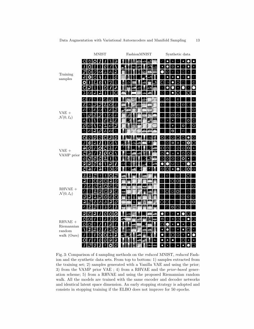
mitigated by the use of a multimodal prior such as the VAMP. However, anotherlimitation of prior-based methods is that they may sample in locations of thelatent space potentially containing very few information (i.e. where no data isavailable). Since the decoder appears to interpolate quite linearly, the classicscheme will generate images which mainly correspond to a superposition of sam-ples (see an example with the red dots in Fig. 2 and the corresponding samplesframed in red). Moreover, there is no way to assess a sample quality before de-coding it and assessing visually its relevance. These limitations may lead to a(very) poor representation of the actual data set diversity while presenting quitea few irrelevant samples. Impressively, sampling along geodesic paths leads tofar more diverse and sharper samples. The new sampling scheme avoids regionsthat have been poorly prospected so that almost every decoded sample is visu-ally satisfying and accounts for the data set diversity. In Fig. 3, we also comparethe models on a reduced MNIST [12] data set composed of 120 samples of 3different classes and a reduced FashionMNIST [21] data set composed again of120 samples from 3 distinct classes. The models are trained with the same neuralnetwork architectures, batch size and learning rate. An early stopping strategyis adopted and consists in stopping training if the ELBO does not improve for 50epochs. As discussed earlier, changing the prior may indeed improve the modelgeneration capacity. For instance samples from the VAE with the VAMP prior(3rd row of Fig. 3) are closer to the training data (1st row of Fig. 3) than withthe Gaussian prior (2nd and 4th row). The model is for instance able to generatecircles when trained with the synthetic data while models using a standard nor-mal prior are not. Nonetheless, a non negligible part of the generated samplesare degraded (see saturated images for the reduced MNIST data for instance).This aspect is mitigated with the proposed generation method which generatesmore diverse and sharper samples.

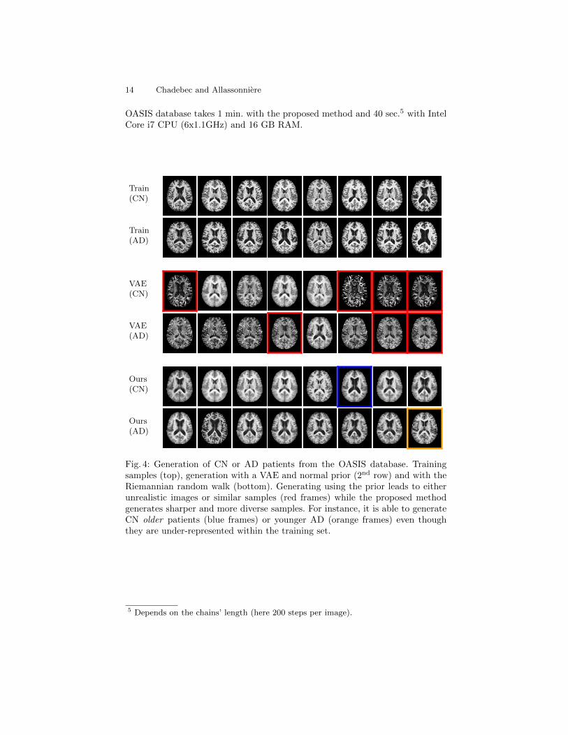
OASIS Database The new generation scheme is then assessed on the publiclyavailable OASIS database composed of 416 patients aged 18 to 96, 100 of whomhave been diagnosed with very mild to moderate Alzheimer disease (AD). AVAE and a RHVAE are then trained to generate either cognitively normal (CN)or AD patients with the same early stopping criteria as before. Fig. 4 showssamples extracted from the training set (top), MRI generated by a vanilla VAE(2nd row) and images from the Riemannian random walk we propose (3rd row).For each method, the upper row shows images of patients diagnosed CN whilethe bottom row presents an AD diagnosis. Again the proposed sampling seemsable to generate a wider range of sharp samples while the VAE appears toproduce non-realistic degraded images which are very similar (see red frames).For example, the proposed scheme allows us to generate realistic old4 patientswith no AD (blue frames) or younger patients with AD (orange frames) eventhough they are under-represented in the training set. Generating 100 images of

4 An older person is characterised by larger ventricles.

Data Augmentation with Variational Autoencoders and Manifold Sampling 13

Trainingsamples

MNIST FashionMNIST Synthetic data

VAE +N (0, Id)

VAE +VAMP prior

RHVAE +N (0, Id)

RHVAE +Riemannianrandomwalk (Ours)

Fig. 3: Comparison of 4 sampling methods on the reduced MNIST, reduced Fash-ion and the synthetic data sets. From top to bottom: 1) samples extracted fromthe training set; 2) samples generated with a Vanilla VAE and using the prior;3) from the VAMP prior VAE ; 4) from a RHVAE and the prior-based gener-ation scheme; 5) from a RHVAE and using the proposed Riemannian randomwalk. All the models are trained with the same encoder and decoder networksand identical latent space dimension. An early stopping strategy is adopted andconsists in stopping training if the ELBO does not improve for 50 epochs.

14 Chadebec and Allassonniere

OASIS database takes 1 min. with the proposed method and 40 sec.5 with IntelCore i7 CPU (6x1.1GHz) and 16 GB RAM.

Train(CN)

Train(AD)

VAE(CN)

VAE(AD)

Ours(CN)

Ours(AD)

Fig. 4: Generation of CN or AD patients from the OASIS database. Trainingsamples (top), generation with a VAE and normal prior (2nd row) and with theRiemannian random walk (bottom). Generating using the prior leads to eitherunrealistic images or similar samples (red frames) while the proposed methodgenerates sharper and more diverse samples. For instance, it is able to generateCN older patients (blue frames) or younger AD (orange frames) even thoughthey are under-represented within the training set.

5 Depends on the chains’ length (here 200 steps per image).

Data Augmentation with Variational Autoencoders and Manifold Sampling 15

Appendix B: Discussion of Remark. 1

Remark 2 If Σ has small enough eigenvalues then Alg. 1 samples from

L(z) =ρS(z)

√det G−1(z)∫

RdρS(z)

√det G−1(z)dz

, (4)

where ρS(z) = 1 if z ∈ S, 0 otherwise, and S is taken as a compact set so thatthe integral is well defined.

If Σ has small enough eigenvalues, it means that the initial velocity v ∼N (0, Σ) will have a low magnitude with high probability. In such a case, we canshow with some approximation that the ratio α in the Riemannian random walkis a Hasting-Metropolis ratio with target density given by Eq. (4). We recall thatthe classic Hasting-Metropolis ratio writes

α(x, y) =π(y)

π(x)· q(x, y)

q(y, x),

where π is the target distribution and q a proposal distribution. In the case ofsmall magnitude velocities, one may show that q is symmetric that is

q(x, y) = q(y, x) .

In our setting, a proposal z is made by computing the geodesic γ starting atγ(0) = z with initial velocity γ(0) = v where v ∼ N (0, Σ) and evaluating it attime 1. First, we remark that γ is well defined since the Riemnanian manifoldM = (R, g) is geodesically complete and γ is unique. Moreover, we have that ←−γis the unique geodesic with initial position ←−γ (0) = z = γ(1) and initial velocity←−γ (0) = −γ(1) and we have

←−γ (t) = γ(1− t), ∀ t ∈ [0, 1] .

In the case of small enough initial velocity, a taylor expansion of the exponentialmay be performed next to 0 ∈ TzM and consists in approximating geodesiccurves with straight lines. That is, for t ∈ [0, 1]

Expz(vt) ≈ z + vt ,

where v = z − z. In such a case we have

γ(t) = v = γ(0) = γ(1) = −←−γ (0) .

Moreover, we have on the one hand

q(z, z) = p(z|z) = p(Expz(v)|z) ' N (z,Σ) .

On the other hand

q(z, z) = p(z|z) = p(Expz(−v)|z) ' N (z, Σ)

16 Chadebec and Allassonniere

Therefore,q(z, z) = q(z, z) .

Finally, the ratio α in the Riemannian random walk may be seen as a Hasting-Metropolis ratio where the target density is given by Eq. (3) and so the algorithmsamples from such a distribution.

Data Augmentation with Variational Autoencoders and Manifold Sampling 17

Appendix C: Computing the Exponential map

To compute the exponential map at any given point p ∈M and for any tangentvector v ∈ TpM we rely on the Hamiltonian definition of geodesic curves. First,for any given v ∈ TpM, the linear form:

qv :

{TpM→ Ru → gp(u, v)

,

is called a moment and is a representation of v in the dual space. In short, wemay write qv(u) = u>Gv. Then, the definition of the Hamiltonian follows

H(p, q) =1

2g∗p(q, q) ,

where g∗p is the dual metric whose local representation is given by G−1(p), theinverse of the metric tensor. Finally, all along geodesic curves the following equa-tions hold

∂p

∂t=∂H

∂q,

∂q

∂t= −∂H

∂p. (5)

Such a system of differential equations may be integrated pretty straight for-wardly using simple numerical schemes such as the second order Runge Kuttaintegration method and Alg. 2 as in [14]. Noteworthy is the fact that such analgorithm only involves one metric tensor inversion at initialization to recoverthe initial moment from the initial velocity. Moreover, it involves closed formoperations since the inverse metric tensor G−1 is known (in our case) and so thegradients in Eq. (5) can be easily computed.

Algorithm 2 Computing the Exponential map

Input: z0 ∈M, v ∈ Tz0M and Tq ← G · vdt← 1

T

for t = 1→ T dopt+ 1

2← pt + 1

2· dt · ∇qH(pt, qt)

qt+ 12← qt − 1

2· dt · ∇pH(pt, qt)

pt+1 ← pt + dt · ∇qH(pt+ 12, qt+ 1

2)

qt+1 ← qt − dt · ∇pH(pt+ 12, qt+ 1

2)

end forReturn pT

18 Chadebec and Allassonniere

Appendix D: VAEs Parameters Setting

Table. 4 summarizes the main hyper-parameters we use to perform the exper-iments presented in the paper while Table. 5 shows the neural networks archi-tectures employed. As to training parameters, we use a Adam optimizer [9] witha learning of 10−3. For the augmentation experiments, we stop training if theELBO does not improve for 20 epochs for all data sets except for OASIS wherethe learning rate is decreased to 10−4 and training is stopped if the ELBO doesnot improve for 50 epochs.

Table 4: RHVAE parameters for each data set.

Data sets Parametersd∗ nlf εlf T λ

√β0

Synthetic 2 3 10−2 0.8 10−3 0.3

reduced Fashion 2 3 10−2 0.8 10−3 0.3

MNIST (bal.) 2 3 10−2 0.8 10−3 0.3

MNIST (unbal.) 2 3 10−2 0.8 10−3 0.3

EMNIST 2 3 10−2 0.8 10−3 0.3

OASIS 2 3 10−3 0.8 10−2 0.3

* Latent space dimension (same for VAE and VAMP-VAE)

Table 5: Neural networks architectures of the VAE, VAMP-VAE and RHVAEfor each data set. The encoder and decoder are the same for all models.

Synthetic, MNIST & Fashion

Net Layer 1 Layer 2 Layer 3

µ∗φ (D, 400, relu)

(400, d, lin.) -Σ∗φ (400, d, lin.) -

π∗θ (d, 400, relu) (400, D, sig.) -

Lψ (diag.)(D, 400, relu)

(400, d, lin.) -

Lψ (low.) (400,d(d−1)

2 , lin.) -

OASIS

µ∗φ (D, 1k, relu) (1k, 400, relu)

(400, d, lin.)Σ∗φ (400, d, lin.)

π∗θ (d, 400, relu) (400, 1k, relu) (1k, D, sig.)

Lψ (diag.)(D, 400, relu)

(400, d, lin.) -

Lψ (low.) (400, d(d−1)2

, lin.) -

* Same for all VAE models

Data Augmentation with Variational Autoencoders and Manifold Sampling 19

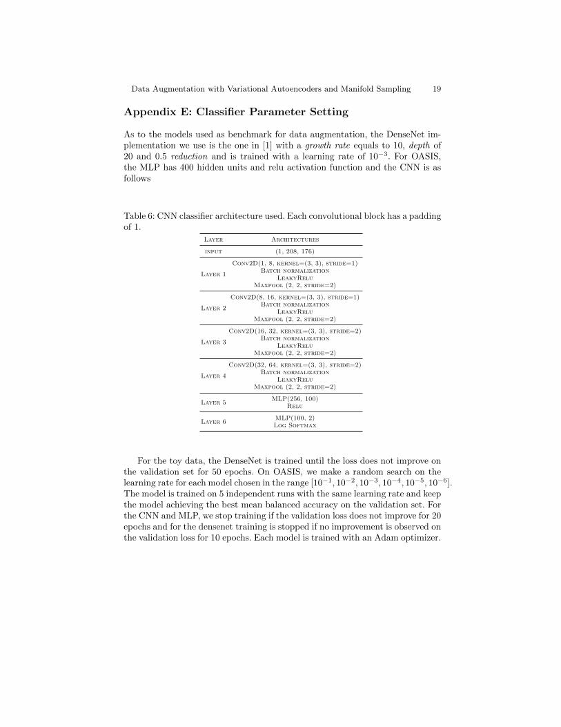
Appendix E: Classifier Parameter Setting

As to the models used as benchmark for data augmentation, the DenseNet im-plementation we use is the one in [1] with a growth rate equals to 10, depth of20 and 0.5 reduction and is trained with a learning rate of 10−3. For OASIS,the MLP has 400 hidden units and relu activation function and the CNN is asfollows

Table 6: CNN classifier architecture used. Each convolutional block has a paddingof 1.

Layer Architectures

input (1, 208, 176)

Layer 1

Conv2D(1, 8, kernel=(3, 3), stride=1)Batch normalization

LeakyReluMaxpool (2, 2, stride=2)

Layer 2

Conv2D(8, 16, kernel=(3, 3), stride=1)Batch normalization

LeakyReluMaxpool (2, 2, stride=2)

Layer 3

Conv2D(16, 32, kernel=(3, 3), stride=2)Batch normalization

LeakyReluMaxpool (2, 2, stride=2)

Layer 4

Conv2D(32, 64, kernel=(3, 3), stride=2)Batch normalization

LeakyReluMaxpool (2, 2, stride=2)

Layer 5MLP(256, 100)

Relu

Layer 6MLP(100, 2)Log Softmax

For the toy data, the DenseNet is trained until the loss does not improve onthe validation set for 50 epochs. On OASIS, we make a random search on thelearning rate for each model chosen in the range [10−1, 10−2, 10−3, 10−4, 10−5, 10−6].The model is trained on 5 independent runs with the same learning rate and keepthe model achieving the best mean balanced accuracy on the validation set. Forthe CNN and MLP, we stop training if the validation loss does not improve for 20epochs and for the densenet training is stopped if no improvement is observed onthe validation loss for 10 epochs. Each model is trained with an Adam optimizer.