FACULTEIT ECONOMIE EN BEDRIJFSWETENSCHAPPEN KU LEUVEN Data analytics for insurance loss modeling, telematics pricing and claims reserving Proefschrift Voorgedragen tot het Behalen van de Graad van Doctor in de Toegepaste Economische Wetenschappen door Roel VERBELEN NUMMER 563 2017

Welcome message from author
This document is posted to help you gain knowledge. Please leave a comment to let me know what you think about it! Share it to your friends and learn new things together.
Transcript

FACULTEIT ECONOMIE ENBEDRIJFSWETENSCHAPPEN
KU LEUVEN
Data analytics for insurance loss modeling,telematics pricing and claims reserving
Proefschrift Voorgedragen tothet Behalen van de Graad vanDoctor in de ToegepasteEconomische Wetenschappen
door
Roel VERBELEN
NUMMER 563 2017


Committee
Advisor:Prof. Dr. Gerda Claeskens KU Leuven
Co-Advisor:Prof. Dr. Katrien Antonio KU Leuven and University of Amsterdam
Chair:Prof. Dr. Robert Boute KU Leuven and Vlerick Business School
Members:Prof. Dr. Jan Beirlant KU Leuven and University of the Free StateProf. Dr. Jan Dhaene KU LeuvenProf. Dr. Edward W. Frees University of Wisconsin–MadisonProf. Dr. Montserrat Guillen University of Barcelona
Daar de proefschriften in de reeks van de Faculteit Economie enBedrijfswetenschappen het persoonlijk werk zijn van hun auteurs, zijn alleen
deze laatsten daarvoor verantwoordelijk.
i

Acknowledgments
“Pursuing a PhD? No thanks, not for me. . . ”
That I needed quite some convincing is something that Katrien will surely confirm.In fact, she already started about 6 years ago when she guided me to the bestpossible educational path after my bachelor studies in mathematics at GhentUniversity. I started wondering about a future career in actuarial science andreached out to Katrien requesting help on the next step to take. I was blownaway by her well-founded and comprehensive reply – that she wrote while beingon vacation. She invited me for a personal meeting at her office in Leuven andconvinced me to switch to KU Leuven and start a master program in statistics.Already back then, she suggested the possibility of afterwards starting a PhD. Assupervisor of my master thesis, she continued to advocate a PhD and togetherwith Gerda eventually persuaded me to embark on an interdisciplinary researchproject, combining actuarial science and statistics. Not a moment has gone bythat I regretted this decision.
First and foremost, I would like to express my profound gratitude to Gerdaand Katrien. During all these years, I have had the privilege to work closely withthem and have them as mentors. Thank you for convincing me to take up thischallenge and supporting me along the way. You were always there for me whenI needed guidance, answered promptly to any of my questions and read articledrafts with the utmost attention to detail. I have been impressed and inspiredby your level of dedication to the university and to research and how you bothmanage to combine it with your family life.
Further, I want to thank my doctoral committee members from KU Leuven(Prof. Jan Beirlant and Prof. Jan Dhaene), my external jury members (Prof. Ed-ward W. Frees and Prof. Montserrat Guillen) and chairman Prof. Robert Boute.Thank you for the thorough reading of my thesis and for all insightful comments
iii

iv Acknowledgements
during the doctoral seminars and preliminary defense. Your constructive sug-gestions helped to improve the quality of this thesis. In particular, thank youProf. Montserrat Guillen for travelling to Leuven to be present at my public de-fense.
I would also like to thank my co-authors of several research papers. Thanksto Prof. Andrei Badescu, Prof. Sheldon Lin and Lan Gong from the Universityof Toronto to introduce me to the class of mixtures of Erlang distributions whichformed the starting point of my research in the field of loss modeling. I’m gratefulfor the collaboration with Tom Reynkens and Prof. Jan Beirlant which lead to arelated follow-up paper. Thank you Jonas Crevecoeur for the joint brainstormsand your feedback on the reserving project. I also very much enjoyed workingwith Maxime Clijsters and Roel Henckaerts on a research topic in the context ofinsurance pricing. I am proud to have co-supervised your master theses whichwere both rewarded with the IA
∣∣BE thesis prize and additionally with the Johande Witt thesis prize for Maxime.
Data have been indispensable for the success of my project in actuarial statis-tics. In this regards, I could benefit from the professional network of Katrien inthe actuarial community and the academic network of Gerda in the statisticalcommunity. Special thanks go out to Jonas Onkelinx for going to great lengthsto share the telematics data with us and for his valuable support in handling thischallenging data set. These telematics data created a strategic advantage andwere of crucial importance for our research on usage-based insurance pricing. Ialso wish to thank Hans Laevens for permission to use the interesting mastitisdata in the multivariate mixture of Erlangs chapter.
I am very grateful to the government agency for Innovation by Science andTechnology (IWT), now called Flanders Innovation & Entrepreneurship (VLAIO),for financing this doctorate and to the Flemish Supercomputer Centre VSC forcomputational support involving simulation studies and analyzing big data sets.
Thanks to KU Leuven for providing me with the facilities to carry out thisdoctoral research. I have enjoyed being part of the stimulating, interactive andinternational research environment that the Faculty of Economics and Businesshas to offer. Since this Faculty hosts both a research group in statistics, as well asin actuarial science, this has been the perfect place to conduct my PhD research.
I am very thankful for having been surrounded by so many nice colleaguesfrom ORSTAT, AFI, LSTAT in Heverlee, down the hall... It has been a pleasureto be part of the statistics group at ORSTAT as well as of the insurance groupat AFI. I have been fortunate to get close with many of you and you formed a

Acknowledgements v
big part in my life over the recent years. Thanks for all those social activitieswe shared together: the barbecues at Thomas’s, the Turkish dinners at Denizand Mehmet’s, Peter’s wedding, the Romania trip for the Pircalabelu wedding,the volleyball games, the soccer with the guys from MSI, the kayaking in theArdennes, organizing the EDC quiz, the nights out at Oude Markt... I haveenjoyed them all very much! In particular, I would like to thank Lore for havingbeen such an incredible office mate. Thanks for all those laughs as well as sincerediscussions on both life and research. I am lucky to have had an office mate whogrew into a close friend. When Lore left for Boston, I was lucky once more to haveDaumantas join the office. Thank you for all those little jokes and creating sucha pleasant working atmosphere. Special thanks go out to Ines for all the advice,support and practical help over the years and for compensating my forgetfulnessfrom time to time.
I want to thank Prof. Meelis Kaarik for the enriching research stay at theUniversity of Tartu in the final months of my doctorate. My office mate Annikahas made me feel very welcome, aitah!
Pursuing a PhD gave me the opportunity to present my work at internationalconferences, to attend scientific workshops and to meet many academics from allover the world. Above all, I was fortunate to have met Liivika in this way. Ourimpressive series of foreign encounters has turned into more than I could everdream of. Thank you for all the wonderful journeys and experiences together. Asa graduating PhD student yourself you understood as no one else how intensivethese doctoral years have been for me and you managed to calm me down wheneverI was stressed. I felt strengthened having you by my side and your support whilewriting this dissertation was invaluable. I’m grateful and proud to have you as apartner in life and I am excited to discover what lies ahead in our future together.
Last but definitely not least I want to thank my family. Words can do nojustice to what you mean to me. You have my deepest and sincerest gratitude foryour encouragement and unconditional support in every step of my life.
Roel Verbelen Leuven, June 2017.

Table of Contents
Committee i
Acknowledgements iii
1 Introduction 11.1 Innovations in loss modeling . . . . . . . . . . . . . . . . . . . . . . 21.2 Innovations in car insurance pricing through telematics technology 41.3 Innovations in claims reserving . . . . . . . . . . . . . . . . . . . . 5
2 Fitting mixtures of Erlangs to censored and truncated data usingthe EM algorithm 92.1 Introduction . . . . . . . . . . . . . . . . . . . . . . . . . . . . . . . 92.2 Mixtures of Erlangs with a common scale parameter . . . . . . . . 132.3 The EM algorithm for censored and truncated data . . . . . . . . . 14
2.3.1 Truncated mixture of Erlangs . . . . . . . . . . . . . . . . . 152.3.2 Construction of the complete data vector . . . . . . . . . . 162.3.3 Initial step . . . . . . . . . . . . . . . . . . . . . . . . . . . 172.3.4 E-step . . . . . . . . . . . . . . . . . . . . . . . . . . . . . . 172.3.5 M-step . . . . . . . . . . . . . . . . . . . . . . . . . . . . . . 20
2.4 Choice of the shape parameters . . . . . . . . . . . . . . . . . . . . 222.4.1 Initialization . . . . . . . . . . . . . . . . . . . . . . . . . . 222.4.2 Adjusting the shapes . . . . . . . . . . . . . . . . . . . . . . 222.4.3 Reducing the number of Erlangs . . . . . . . . . . . . . . . 232.4.4 Compare the resulting fit using different initializing param-
eters . . . . . . . . . . . . . . . . . . . . . . . . . . . . . . . 242.5 Examples . . . . . . . . . . . . . . . . . . . . . . . . . . . . . . . . 25
2.5.1 Simulated censored and truncated bimodal data . . . . . . 25
vii

viii Table of Contents
2.5.2 Unemployment duration . . . . . . . . . . . . . . . . . . . . 292.5.3 Secura Re, Belgian insurance data . . . . . . . . . . . . . . 312.5.4 Simulated generalized Pareto data . . . . . . . . . . . . . . 35
2.6 Discussion . . . . . . . . . . . . . . . . . . . . . . . . . . . . . . . . 382.7 Appendix A: Denseness . . . . . . . . . . . . . . . . . . . . . . . . 392.8 Appendix B: Partial derivative of Q . . . . . . . . . . . . . . . . . 39
3 Multivariate mixtures of Erlangs for density estimation undercensoring 433.1 Introduction . . . . . . . . . . . . . . . . . . . . . . . . . . . . . . . 433.2 Multivariate Erlang mixtures with a common scale parameter . . . 463.3 Parameter estimation . . . . . . . . . . . . . . . . . . . . . . . . . 48
3.3.1 Randomly censored and fixed truncated data . . . . . . . . 483.3.2 Construction of the complete data likelihood . . . . . . . . 503.3.3 The EM algorithm for censored and truncated data . . . . 51
3.4 Computational details . . . . . . . . . . . . . . . . . . . . . . . . . 543.4.1 Initialization and first run of the EM algorithm . . . . . . . 543.4.2 Reduction of the shape vectors . . . . . . . . . . . . . . . . 573.4.3 Adjustment of the shape vectors . . . . . . . . . . . . . . . 59
3.5 Examples . . . . . . . . . . . . . . . . . . . . . . . . . . . . . . . . 613.5.1 Simulated data . . . . . . . . . . . . . . . . . . . . . . . . . 613.5.2 Old faithful geyser data . . . . . . . . . . . . . . . . . . . . 653.5.3 Mastitis study . . . . . . . . . . . . . . . . . . . . . . . . . 68
3.6 Discussion . . . . . . . . . . . . . . . . . . . . . . . . . . . . . . . . 713.7 Appendix: Partial derivative of Q . . . . . . . . . . . . . . . . . . . 72
4 Unraveling the predictive power of telematics data in car insur-ance pricing 754.1 Introduction . . . . . . . . . . . . . . . . . . . . . . . . . . . . . . . 764.2 Statistical background and related modeling literature . . . . . . . 794.3 Telematics insurance data . . . . . . . . . . . . . . . . . . . . . . . 81
4.3.1 Data processing . . . . . . . . . . . . . . . . . . . . . . . . . 814.3.2 Risk classification using policy and telematics information . 85
4.4 Model building and selection . . . . . . . . . . . . . . . . . . . . . 894.4.1 Generalized additive models . . . . . . . . . . . . . . . . . . 904.4.2 Compositional data . . . . . . . . . . . . . . . . . . . . . . 914.4.3 Model selection and assessment . . . . . . . . . . . . . . . . 97
4.5 Results . . . . . . . . . . . . . . . . . . . . . . . . . . . . . . . . . . 99

Table of Contents ix
4.5.1 Model selection . . . . . . . . . . . . . . . . . . . . . . . . . 994.5.2 Model assessment . . . . . . . . . . . . . . . . . . . . . . . . 1014.5.3 Visualization and discussion . . . . . . . . . . . . . . . . . . 103
4.6 Conclusion . . . . . . . . . . . . . . . . . . . . . . . . . . . . . . . 1074.7 Appendix A: Structural zero patterns of the compositional telem-
atics predictors . . . . . . . . . . . . . . . . . . . . . . . . . . . . . 1094.8 Appendix B: Functional forms of the selected best models . . . . . 1114.9 Appendix C: Graphical model displays . . . . . . . . . . . . . . . . 1124.10 Appendix D: Relative importance . . . . . . . . . . . . . . . . . . . 115
5 Predicting daily IBNR claim counts using a regression approachfor the occurrence of claims and their reporting delay 1195.1 Introduction . . . . . . . . . . . . . . . . . . . . . . . . . . . . . . . 1205.2 Data and first insights . . . . . . . . . . . . . . . . . . . . . . . . . 1245.3 The statistical model . . . . . . . . . . . . . . . . . . . . . . . . . . 129
5.3.1 Daily claim count data . . . . . . . . . . . . . . . . . . . . . 1295.3.2 Model assumptions . . . . . . . . . . . . . . . . . . . . . . . 1305.3.3 Parameter estimation using the EM algorithm . . . . . . . 1325.3.4 Asymptotic variance-covariance matrix . . . . . . . . . . . . 1375.3.5 Prediction of IBNR claim counts . . . . . . . . . . . . . . . 139
5.4 Results . . . . . . . . . . . . . . . . . . . . . . . . . . . . . . . . . . 1395.4.1 Parameter estimates . . . . . . . . . . . . . . . . . . . . . . 1405.4.2 Prediction of IBNR claim counts . . . . . . . . . . . . . . . 1435.4.3 Prediction of total IBNR claim counts over time . . . . . . 145
5.5 Conclusions and outlook . . . . . . . . . . . . . . . . . . . . . . . . 1475.6 Appendix: Derivation of the asymptotic variance-covariance matrix 148
6 Outlook 1536.1 Further developments in loss modeling . . . . . . . . . . . . . . . . 1536.2 Further developments in telematics insurance . . . . . . . . . . . . 1556.3 Further developments in claims reserving . . . . . . . . . . . . . . 157
List of Figures 164
List of Tables 167
Bibliography 181
Doctoral dissertations of the Faculty of Economics and Business 183

Chapter 1
Introduction
Today’s society generates data more rapidly than ever before, creating manyopportunities as well as challenges for statisticians. Many industries become in-creasingly dependent on high-quality data, and the demand for sound statisticalanalysis of these data is rising accordingly.
In the insurance sector, data have always played a major role. When sellinga contract to a client, the insurance company is liable for the claims arising fromthis contract and will hold capital aside to meet these future liabilities. As such,the insurance premium has to be paid before the real costs are known. This isreferred to as the inversion of the production cycle. It implies that the activitiesof pricing and reserving are strongly interconnected in actuarial practice. Onthe one hand, pricing actuaries have to determine a fair price for the insuranceproducts they want to sell. Setting the premium levels charged to the insuredsis done in a data driven way where statistical models are essential. Risk-basedpricing is crucial in a competitive and well-functioning insurance market. Onthe other hand, an insurance company must safeguard its solvency and reservecapital to fulfill outstanding liabilities. Reserving actuaries thus must predict,with maximum accuracy, the total amount needed to pay claims that the insurerhas legally committed himself to cover for. These reserves form the main itemon the liability side of the balance sheet of the insurance company and thereforehave an important economic impact.
The ambition of this research is the development of new, accurate predictivemodels for the actuarial work field. Non-life (e.g. motor, fire, liability), life andhealth insurers are constantly confronted with the challenges created by rapidlyincreasing computer facilities for data collection, storage and analysis. However,
1
2 Introduction
using their state-of-the-art methodologies the insurance business will not be ableto formulate an adequate response to these challenges, and interactions with thedisciplines of statistics and big data analytics are necessary. Moreover, the in-creased focus on internal risk management and the changing supervisory guide-lines motivate the relevance of improved tools for actuarial predictive modeling.In particular, the European Solvency II Directive1 imposes new solvency require-ments to enhance policyholder protection. With the recent introduction of thesenew regulatory guidelines, the measurement of future cash flows and their uncer-tainty becomes more important. At the same time, actuarial predictive modelshave to comply with existing and pending regulations. The Gender Directive2
has prohibited the use of gender as a risk factor in insurance pricing and antidis-crimination laws may progress in the near future further limiting the contractualfreedom of insurance companies.
The overall objective in this work is to improve actuarial practices for pricingand reserving by using sound and flexible statistical methods shaped for the actu-arial data at hand. The tools we develop should lead to a better understanding ofactuarial risks and an improved risk management. This thesis focuses on three re-lated research avenues in the domain of non-life insurance: (1) flexible univariateand multivariate loss modeling in the presence of censoring and truncation, (2)car insurance pricing using telematics data and (3) micro-level claims reserving.
1.1 Innovations in loss modeling
Modeling claim losses – also called claim sizes or severities – is crucial when pricinginsurance products, determining capital requirements, or managing risks withinfinancial institutions. Various basic continuous distributions, such as the gammaor lognormal, have been employed to model nonnegative losses. However, theseparametric distributions are not always appropriate for actuarial data, which maybe multimodal or heavy-tailed. Furthermore, when constructing collective riskmodels or combining actuarial risks from multiple lines of business, these severitydistributions do not lead to an analytical form for the corresponding aggregateloss distribution. While numerical or simulation algorithms are available, it isnevertheless convenient to utilize analytical techniques when possible. Of course,there is always a tradeoff between mathematical simplicity on the one hand andrealistic modeling on the other. Ideally, loss models require on the one hand the
1 See http://eur-lex.europa.eu/legal-content/EN/ALL/?uri=CELEX:32009L0138.2 See http://europa.eu/rapid/press-release_IP-12-1430_en.htm.
1.1. Innovations in loss modeling 3
flexibility of nonparametric approaches to describe the claims and on the otherhand the feasibility to analytically quantify the risk.
In actuarial literature, the use of mixtures of Erlang distributions with a com-mon scale parameter has been suggested to model insurance losses. An Erlangdistribution is in fact a gamma distribution with an integer shape parameter andcan be decomposed as the sum of independent, exponentially distributed randomvariables with the same mean (equal to the inverse of the scale parameter). A mix-ture of such distributions with a common scale parameter can be considered as acompound distribution of a random sum of exponential random variables with thesame mean. The resulting class of distributions enjoys a wide variety of analyticproperties because it can exploit the mathematical tractability of the exponentialdistribution. Many quantities of interest in connection with the aggregation ofclaims and stop-loss analysis are easily computable under the mixture of Erlangsassumption. At the same time, mixtures of Erlangs are extremely versatile interms of possible shapes of the probability density function and are capable ofmultimodality as well as a wide range of degrees of skewness in the right tail,often the region of particular interest for risk management purposes. In fact, thisclass of distributions is dense in the space of positive continuous distributions. Assuch, any continuous distribution can be approximated to an arbitrary degree ofaccuracy by a mixture of Erlang distribution.
In Chapter 2, we discuss how to estimate mixtures of Erlangs using censoredand truncated data. Parameter estimation is of course of utmost importancewhen we want to apply these mixtures of Erlangs in real-life applications. Ourwork is further inspired by the omnipresence of censoring and truncation in anactuarial context. Insurance contracts often do not provide full coverage of aloss. A policy modification such as a (franchise) deductible of e500 causes theinsurer to only pay for the claim if it exceeds e500. Such kind of deductible isalso used in excess-of-loss reinsurance treaties when an insurance company on histurn buys protection for a certain loss layer. As a consequence, only paymentsthat exceed this threshold will be recorded by the reinsurer and can be used toestimate the loss distribution. The insurance losses are said to be left truncatedat that threshold. Policy limits on the other hand define the maximum amountof coverage provided by the insurer. This policy modification has as effect thatthe observed insurance losses are right censored, meaning that the exact value ofthe loss, in case it exceeds this limit, is not recorded. Right censoring also ariseswhen claims are not yet fully settled. For such unsettled claims only the paymentto date is known whereas the final total payment will be at least as much.
4 Introduction
In Chapter 3, we extend the estimation procedure under censoring and trun-cation to multivariate mixtures of Erlang distributions. This multivariate distri-bution generalizes the univariate mixture of Erlang distributions while preservingits flexibility and analytical tractability. When modeling multivariate insurancelosses or dependent risks from different portfolios or lines of business, the inherentshape versatility of multivariate mixtures of Erlangs allows one to adequately cap-ture both the marginals and the dependence structure. Moreover, its desirableanalytical properties are particularly convenient in a wide variety of insurancerelated modeling situations.
1.2 Innovations in car insurance pricing throughtelematics technology
Telematics technology – the integrated use of telecommunication and informatics– may fundamentally change the car insurance industry by allowing insurers tobase their prices on the real driving behavior instead of on traditional policyholdercharacteristics and historical claims information. The use of this technology ininsured vehicles enables to transmit and receive information that allows an insur-ance company to better assess the accident risk of drivers and adjust the premiumsaccordingly through usage-based insurance. A small black box device is installedin the insured’s car containing a GPS system, electronics that capture hundredsof sensor inputs, a SIM card and some computer software. It records the drivingbehavior directly and shares this information with the insurer.
On February 23, 2013 The Economist3 reported “Underwriters have tradition-ally used crude demographic data such as age, location and sex to separate thetestosterone-fueled boy racers from their often tamer female counterparts. Nowtechnology is giving insurers the chance to see just how skilled a driver really is.By monitoring their customers’ motoring habits, underwriters can increasinglydistinguish between drivers who are safe on the road from those who merely seemsafe on paper. Many think that ‘telematics insurance’ will become the industrynorm.”
This industry (r)evolution creates multiple opportunities from a business aswell as statistical modeling perspective. With telematics insurance focus will beon how much time a car spends on the road (pay-as-you-drive) or on driver ability(pay-how-you-drive), as an alternative for the current practice where observable
3 How’s my driving? (2013, February 23) The Economist. http: // econ. st/ Yd5x3C
1.3. Innovations in claims reserving 5
risk information (like age or gender) is used as a proxy for unobservable character-istics (like distance driven or driving style). The upswing of telematics data mayalso replace (in the near future) rating variables which are currently being bannedfrom actuarial pricing practice by recent court decisions (such as the gender ban).
The availability of such data collected while driving creates a wide, but unex-plored territory for statisticians. Usage-based insurance forces pricing actuariesto change their current practice and to develop innovative statistical tools to cus-tomize premiums based on the actual driving behavior. Analytic contributionson this topic in scientific research are scarce, probably because the collection ofthis type of data is immature and brand new.
In Chapter 4, we explore the vast potential of telematics insurance from astatistical point of view by analyzing a unique Belgian portfolio. Driving behaviordata are collected in between 2010 and 2014 for young drivers who signed up fora telematics product. Since 2010, the Belgian insurance company offers youngdrivers a premium discount in exchange for a black box to be installed in theircar. This telematics device collects data on when, where and how long the car isbeing used. The aim of our contribution is to develop the statistical methodologyto incorporate this telematics information in statistical rating models, where wefocus on predicting the number of claims, in order to adequately set premiumlevels based on individual policyholder’s driving habits. We propose new toolsand techniques that actuaries can use to improve their current pricing practicesand to design new products that are better aligned with the potential these newtechnologies offer.
1.3 Innovations in claims reserving
To be able to fulfill future liabilities insurance companies will hold sufficient cap-ital reserves. Loss reserving deals with the prediction of the remaining develop-ment of reported, open claims (reported but not settled reserve) and unreportedclaims (incurred but not reported reserve). Accurate, reliable and robust reservingmethods for a wide range of products and lines of business are key factors in thestability and solvability of insurance companies. The industry-wide standard isthe chain-ladder technique, which works on data aggregated in a run-off triangle.A run-off triangle summarizes the information registered during the lifetime ofindividual claims by aggregating loss payments over two dimensions, namely theyear of occurrence of the claim and the period since claim event during which thepayment took place.
6 Introduction
Nowadays, insurance companies keep track of detailed information for eachindividual claim. Rich data sources record, for example, the occurrence date, thereporting delay, the date and amount of each loss payment, and the settlementdate. The existing methods for claims reserving are designed for aggregated data,but through this data compression many useful information is lost. With theadvent of Solvency II, insurers are required to not only provide a best estimate oftheir future liabilities, but also to have a better grasp of their uncertainty. Currenttechniques for loss reserving will have to be improved, adjusted or extended tomeet the requirements of the new regulations.
In Chapter 5, we leave the track of aggregated data and focus on the un-derlying, more granular data. Stochastic loss reserving methods designed at theindividual claim level are referred to as micro-level reserving techniques. The over-all goal is to increase the predictive power of loss reserving methods and improverisk measurement by using the information stored in the insurer’s data base sys-tem, instead of ignoring it. We focus on modeling the claims arrival and reportingdelay using a micro-level approach. Due to time delays between the occurrenceof the insured event and the notification of the claim to the insurer, not all of theclaims that occurred in the past have been observed when the reserve needs tobe calculated. We present a flexible regression framework to model and jointlyestimate the occurrence and reporting of claims. This new technique models theclaim arrival process on a daily basis in order to predict the number of incurredbut not reported claim counts.
The various chapters in this thesis can be found in
(i) Verbelen, R., Gong, L., Antonio, K., Badescu, A., and Lin, X. S. (2015).Fitting mixtures of Erlangs to censored and truncated data using the EMalgorithm. ASTIN Bulletin, 45(3):729-758.
(ii) Verbelen, R., Antonio, K., and Claeskens, G. (2016). Multivariate mixturesof Erlangs for density estimation under censoring. Lifetime Data Analysis,22(3):429-455.
(iii) Verbelen, R., Antonio, K., and Claeskens, G. (2016). Unraveling the pre-dictive power of telematics data in car insurance pricing. FEB ResearchReport KBI 1624.
(iv) Verbelen, R., Antonio, K., Claeskens, G. and Crevecoeur, J. (2017). Predict-ing daily IBNR claim counts using a regression approach for the occurrenceof claims and their reporting delay. Working paper.

1.3. Innovations in claims reserving 7
The author also contributed to the following original publications
(i) Reynkens, T., Verbelen, R., Beirlant, J. and Antonio, K. (2016). Modelingcensored losses using splicing: a global fit strategy with mixed Erlang andextreme value distributions, arXiv:1608.01566.
(ii) Henckaerts, R., Antonio, K., Clijsters, M. and Verbelen, R. (2017). A datadriven binning strategy for the construction of risk classes, Working paper.

Chapter 2
Fitting mixtures of Erlangs to
censored and truncated data using
the EM algorithm
Abstract
We discuss how to fit mixtures of Erlangs to censored and truncated databy iteratively using the EM algorithm. Mixtures of Erlangs form a very ver-satile, yet analytically tractable, class of distributions making them suitablefor loss modeling purposes. The effectiveness of the proposed algorithm isdemonstrated on simulated data as well as real data sets.
This chapter is based on Verbelen, R., Gong, L., Antonio, K., Badescu, A., andLin, X. S. (2015). Fitting mixtures of Erlangs to censored and truncated datausing the EM algorithm. ASTIN Bulletin, 45(3):729-758
2.1 Introduction
The class of mixtures of Erlang distributions with a common scale parameter isvery flexible in terms of the possible shapes of its members. Tijms (1994, p. 163)shows that mixtures of Erlangs are dense in the space of positive distributionsin the sense that there always exists a series of mixtures of Erlangs that weaklyconverges, i.e. converges in distribution, to any positive distribution. As such, anycontinuous distribution can be approximated by a mixture of Erlang distributions
9
10 Mixtures of Erlangs
to any accuracy. Furthermore, via direct manipulation of the Laplace transform,a wide variety of distributions whose membership in this class is not immediatelyobvious can be written as a mixture of Erlangs. The class of mixtures of Erlangswith a common scale is also closed under mixture, convolution and compounding.At the same time, it is possible to work analytically with this class leading toexplicit expressions for e.g. the Laplace transform, the hazard rate, a Tail-Value-at-Risk (TVAR) and stop-loss moments. A quantile or a Value-at-Risk (VaR)can be obtained by numerically inverting the cumulative distribution function.Klugman et al. (2013), Willmot and Lin (2011) and Willmot and Woo (2007)give an overview of these analytical and computational properties of mixtures ofErlangs.
Mixtures of Erlang distributions have received most attention in the field ofactuarial science. Modeling data on claim sizes is crucial when pricing insuranceproducts. Actuarial models help insurance companies to assess the risk associatedwith the portfolio, to set the level of premiums (Frees and Valdez, 2008) and re-serves (Antonio and Plat, 2014), to determine optimal reinsurance levels (Beirlantet al., 2004) or to determine capital requirements for solvency purposes (Bolanceet al., 2012). Insurance data are often modeled using a parametric distributionsuch as a gamma, lognormal or Pareto distribution. The usual way to proceedin loss modeling, pricing and reserving is to calibrate the data using several ofthese parametric distributions and then select, among these, the most appropriatemodel based on a model selection tool (Klugman and Rioux, 2006). These classesof distributions may however not always be flexible enough in terms of the possibleshapes of their members in order to obtain a satisfying fit (e.g. in the presence ofmultimodal data) and resulting models become intractable when aggregating risksin an insurance portfolio or arising from multiple lines of losses. Ideally, it wouldbe useful to have a single approach to fitting loss models (Klugman and Rioux,2006) with on the one hand the flexibility of nonparametric density estimationtechniques to describe the insurance losses and on the other hand the feasibilityto analytically quantify the risk. This is exactly what the class of mixtures of Er-langs has to offer. In particular, using these distributions in aggregate loss modelsleads to an analytical form of the corresponding aggregate loss distribution, whichavoids the need for simulations to evaluate the model.
Mixture models are often used to reflect the heterogeneity in a populationconsisting of multiple groups or clusters (McLachlan and Peel, 2001). In someapplications, these clusters can be physically identified and used to interpret thefitted distributions. This is however not the approach we follow; the components
2.1. Introduction 11
in the mixture will not be identified with existing groups. Mixtures of Erlangs arediscussed here for their great flexibility in modeling data and should be regardedas a semiparametric density estimation technique. The densities in the mixtureare parametrically specified as Erlangs, whereas the associated weights form thenonparametric part. The number of Erlangs in the mixture with non-zero weightscan be viewed as a smoothing parameter. Mixtures of Erlangs have much ofthe flexibility of nonparametric approaches and furthermore allow for tractableresults.
The expectation-maximization (EM) algorithm, first introduced by Dempsteret al. (1977), is an iterative method used to compute maximum likelihood (ML)estimates when the data can be viewed as being incomplete and direct maxi-mization of the incomplete data likelihood is either not desirable or not possible(McLachlan and Krishnan, 2008). The EM algorithm is particularly useful inestimating the parameters of a finite mixture. The clue is to view data from amixture as being incomplete since the associated component-label vectors are notavailable (McLachlan and Peel, 2001).
Lee and Lin (2010) iteratively use the EM algorithm (Dempster et al., 1977)for finite mixtures to estimate the parameters of a mixture of Erlang distributionswith a common scale parameter. For a specified fixed set of shapes, the E- andM-step can be solved analytically without using any optimization method. Thismakes the EM algorithm for mixtures of Erlangs a pure iterative algorithm whichis therefore simple, effective and easy to implement. The initialization is basedon Tijm’s proof of the denseness property of mixtures of Erlangs (Tijms, 1994,p. 163) which ensures good starting values and fast convergence. Since the numberof Erlangs in the mixture and the corresponding shape parameters are pre-fixedand hence not estimated, Lee and Lin (2010) propose an adjustment procedureto identify the ‘optimal’ number of Erlang distributions and the ‘optimal’ shapeparameters of these distributions in the mixture. The authors illustrate the flex-ibility of mixtures of Erlangs by generating data from parametric models (suchas the uniform, lognormal, and generalized Pareto distribution) and by approx-imating the underlying distribution of this sample using a mixture of Erlangs.They further demonstrate the usefulness of mixtures of Erlangs in the contextof quantitative risk management for the insurance business. However, modelingcensored and/or truncated losses is not covered by the approach in Lee and Lin(2010).
In many practical problems data are censored and/or truncated, for example,due to the way how the data is collected or measured or by the design of the
12 Mixtures of Erlangs
experiment. Censoring entails that you only know in which interval an observationof a variable lies without knowing the exact value while truncation implies thatyou only observe values that lie within a given range. Interest however is in theunderlying distribution of the uncensored and untruncated data instead of theobserved censored and/or truncated data. Hence the censoring and truncationhas to be accounted for in the analysis.
Survival analysis is the most common application in which data are oftencensored and truncated. A typical example is a medical study in which one followspatients over a period of time. In case the event of interest has not yet occurredbefore the end of the study, the patient drops out of the study or dies from anothercause, independent of the cause of interest, the event time is right censored. Incase the event of interest is known to have occurred between two dates, but theprecise date is not known, the event time is interval censored. In actuarial science,insurance losses are often censored and truncated due to policy modifications suchas deductibles (left truncation) and policy limits (right censoring). Left truncationis also present in life insurance where members of pension schemes and holders ofinsurance contracts only enter a portfolio at a certain adult age. Censored andtruncated data occur in the context of claim reserving as well (Antonio and Plat,2014). Indeed, the reserving actuary wants to predict the future development ofclaims when setting aside reserves at the present moment and has to deal withclaims being reported but not yet settled (RBNS) and claims being incurred butnot yet reported (IBNR). In operational risk, data are left truncated as they areonly recorded in case they exceed a certain threshold. Badescu et al. (2015) use theEM algorithm to fit the correlated frequencies of such left truncated operationalloss data using an Erlang-based multivariate mixed Poisson distribution.
Motivated by the large number of areas where censored and truncated dataare encountered, the objective in this chapter is to develop an extension of theiterative EM algorithm of Lee and Lin (2010) for fitting mixtures of Erlangs withcommon scale parameter to censored and truncated data. The traditional wayof dealing with (grouped and) truncated data using the EM algorithm involvestreating the unknown number of truncated observations as a random variable andincluding it into the complete data vector (Dempster et al., 1977; McLachlan andKrishnan, 2008, p. 66; McLachlan and Peel, 2001, p. 257; McLachlan and Jones,1988). We do not follow this approach and rather only include the uncensoredobservations and the component-label vectors in the complete data vector as is alsodone in Lee and Scott (2012). The fitting procedure is applicable to a wide rangeof applications. We demonstrate its use in actuarial science and econometrics.

2.2. Mixtures of Erlangs with a common scale parameter 13
In the following, we briefly introduce mixtures of Erlangs with a commonscale parameter in Section 2.2. The adjusted EM algorithm, able to deal withcensored and truncated data, is presented in Section 2.3. The procedures usedto initialize the parameters, to adjust the shapes of the Erlangs in the mixtureand to choose the number of components are discussed in Section 2.4. Examplesfollow in Section 2.5 and Section 2.6 concludes.
2.2 Mixtures of Erlangs with a common scale pa-rameter
The Erlang distribution is a positive continuous distribution with density function
f(x; r, θ) = xr−1e−x/θ
θr(r − 1)! for x > 0 , (2.1)
where r, a positive integer, is the shape parameter and θ > 0 the scale parameter(the inverse λ = 1/θ is called the rate parameter). The cumulative distributionfunction is obtained by integrating (2.1) by parts r times
F (x; r, θ) =∫ x
0
zr−1e−z/θ
θr(r − 1)! dz = 1−r−1∑n=0
e−x/θ (x/θ)n
n! . (2.2)
Following Lee and Lin (2010) we consider mixtures of M Erlang distributionswith common scale parameter θ > 0 and having density
f(x;α, r, θ) =M∑
j=1αj
xrj−1e−x/θ
θrj (rj − 1)! =M∑
j=1αjf(x; rj , θ) for x > 0 , (2.3)
where the positive integers r = (r1, . . . , rM ) with r1 < . . . < rM are the shapeparameters of the Erlang distributions and α = (α1, . . . , αM ) with αj > 0 and∑M
j=1 αj = 1 are the weights used in the mixture. Similarly, the cumulativedistribution function can be written as a weighted sum of terms (2.2) or (2.22).
Tijms (1994, p. 163) shows that the class of mixtures of Erlang distributionswith a common scale parameter is dense in the space of distributions on R+. Theformulation of the Theorem is given in Appendix 2.7. Lee and Lin (2010) give analternative proof using characteristic functions.
14 Mixtures of Erlangs
2.3 The EM algorithm for censored and trun-cated data
Lee and Lin (2010) formulate the EM algorithm customized for fitting mixturesof Erlangs with a common scale parameter to complete data. Here, we constructan adjusted EM algorithm which is able to deal with censored and truncateddata. We represent a censored sample truncated to the range [tl, tu] by X ={ (li, ui)| i = 1, . . . , n}, where tl and tu represent the lower and upper truncationpoints, li and ui the lower and upper censoring points and tl 6 li 6 ui 6 tu
for i = 1, . . . , n. tl = 0 and tu = ∞ mean no truncation from below and above,respectively. The censoring status is determined as follows:
Uncensored: tl 6 li = ui =: xi 6 tu
Left Censored: tl = li < ui < tu
Right Censored: tl < li < ui = tu
Interval Censored: tl < li < ui < tu
For example, when the truncation interval equals [tl, tu] = [0, 10], an uncen-sored observation at 1 gets denoted by (li, ui) = (1, 1), an observation left censoredat 2 by (li, ui) = (0, 2), an observation right censored at 3 by (li, ui) = (3, 10)and an observation censored between 4 and 5 by (li, ui) = (4, 5). Thus, li andui should be seen as the lower and upper endpoints of the interval that containsobservation i.
The parameter vector to be estimated is Θ = (α, θ). The number of ErlangsM in the mixture and the corresponding positive integer shapes r are fixed. Thevalue of M is, in most applications, however unknown and has to be inferred fromthe available data, along with the shape parameters, see Section 2.4. The portionof the likelihood containing the unknown parameter vector Θ is given by
L(Θ;X ) =∏i∈U
f(xi; Θ)F (tu; Θ)− F (tl; Θ)
∏i∈C
F (ui; Θ)− F (li; Θ)F (tu; Θ)− F (tl; Θ)
where U is the subset of observations in {1, . . . , n} which are uncensored and C
is the subset of left, right and interval censored observations. In case there is notruncation, i.e. [tl, tu] = [0,∞], the contribution of a left censored observation tothe likelihood equals F (ui; Θ) since li = 0, of a right censored observation 1 −F (li; Θ) with ui =∞, and of an interval censored observation F (ui; Θ)−F (li; Θ).

2.3. The EM algorithm for censored and truncated data 15
The corresponding log-likelihood is
l(Θ;X ) =∑i∈U
ln
M∑j=1
αjf(xi; rj , θ)
+∑i∈C
ln
M∑j=1
αj (F (ui; rj , θ)− F (li; rj , θ))
− n ln
M∑j=1
αj
(F (tu; rj , θ)− F (tl; rj , θ)
) , (2.4)
which is difficult to optimize numerically.
2.3.1 Truncated mixture of Erlangs
The probability density function evaluated at an uncensored observation xi aftertruncation (tl, tu) is given by
f(xi; tl, tu, Θ) = f(xi; Θ)F (tu; Θ)− F (tl; Θ)
=M∑
j=1αj ·
f(xi; rj , θ)F (tu; Θ)− F (tl; Θ)
=M∑
j=1αj ·
F (tu; rj , θ)− F (tl; rj , θ)F (tu; Θ)− F (tl; Θ) · f(xi; rj , θ)
F (tu; rj , θ)− F (tl; rj , θ)
=M∑
j=1βjf(xi; tl, tu, rj , θ) , (2.5)
for tl 6 xi 6 tu and zero otherwise. This is again a mixture with mixing weightsβj and component density functions given by, respectively,
βj = αj ·F (tu; rj , θ)− F (tl; rj , θ)
F (tu; Θ)− F (tl; Θ) (2.6)
and
f(xi; tl, tu, rj , θ) = f(xi; rj , θ)F (tu; rj , θ)− F (tl; rj , θ) . (2.7)
The component density functions f(xi; tl, tu, rj , θ) are truncated versions of theoriginal component density functions f(xi; rj , θ). The weights βj are obtained byreweighting the original weights αj by means of the probabilities of the corre-sponding component to lie in the truncation interval.
16 Mixtures of Erlangs
2.3.2 Construction of the complete data vector
The EM algorithm provides a computationally easy way to fit this finite mixtureto the censored and truncated data. The main clue is to regard the censoredsample X as being incomplete since the uncensored observations x = (x1, . . . , xn)and their associated component-indicator vectors z = (z1, . . . , zn) with
zij =
1 if observation xi comes from the mixture component (2.7)
corresponding to the shape parameter rj
0 otherwise
(2.8)
for i = 1, . . . , n and j = 1, . . . , M , are not available. The component-label vectorsz1, . . . , zn are distributed according to a multinomial distribution consisting ofone draw on M categories with probabilities β1, . . . , βM where
P (Zi = zi) = βzi11 . . . , βziM
M
for i = 1, . . . , n with zij equal to 0 or 1 and∑M
j=1 zij = 1. We write
Z1, . . . ,Zni.i.d.∼ MultM (1,β) .
Hence, the latent variables Zi reveal which component density generated obser-vation xi. Whereas the unconditional truncated probability density function isgiven by (2.5), the conditional truncated probability density function of Xi givenZij = 1 is given by (2.7).
The complete data vector, Y = (x1, . . . , xn, z) = {(xi, zi)|i = 1 . . . n}, containsall uncensored observations xi and their corresponding mixing component vectorzi. The log-likelihood of the complete sample Y then becomes
l(Θ;Y) =n∑
i=1
M∑j=1
zij ln(βjf(xi; tl, tu, rj , θ)
), (2.9)
which has a simpler form than the incomplete log-likelihood (2.4) as it does notcontain logarithms of sums. The EM algorithm deals with the censored andtruncated data from the mixture of Erlangs with common scale in the followingsteps.

2.3. The EM algorithm for censored and truncated data 17
2.3.3 Initial step
An initial guess for Θ is needed to start the algorithm. The closer the startingvalue is to the true maximum likelihood estimator, the faster the algorithm willconverge. Parameter initialization is often the sore point of an EM implementationand the study of good initial estimates is often not feasible and disregarded.
For mixtures of Erlangs however, the denseness property (see Tijms (1994,p. 163) and Appendix 2.7) provides an excellent way of coming up with goodinitial estimates. In the initial step, we deal with the censoring and truncationin a crude manner. We switch to an initializing data set, denoted by d, in whichwe treat the left and right censored data points as being observed, i.e. we useui and li, respectively, and we replace the interval censored data points with themidpoint, i.e. we use (li + ui)/2. Based on this initial data, we initialize theparameters θ and α as:
θ(0) = max(d)rM
and α(0)j =
∑ni=1 I
(rj−1θ(0) < di 6 rjθ(0))
n, (2.10)
for j = 1, . . . , M , with r0 = 0 for notational convenience. Inspired by Tijms’s for-mulation of the denseness property, the initial scale θ(0) is chosen such that θ(0)rM
equals the maximum data point and the initial weights αj for j = 1, 2, . . . , M areset to be the relative frequency of data points in the interval (rj−1θ(0), rjθ(0)].The truncation is only taken into account to transform the initial values for αinto the initial values for β via (2.6).
2.3.4 E-step
In the kth iteration of the E-step, we take the conditional expectation of thecomplete log-likelihood (2.9) given the incomplete data X and using the currentestimate Θ(k−1) for Θ with
Q(Θ; Θ(k−1)) = E(l(Θ;Y) | X ; Θ(k−1))
= E
∑i∈U
M∑j=1
Zij ln(βjf(xi; tl, tu, rj , θ)
)∣∣∣∣∣∣X ; Θ(k−1)
+ E
∑i∈C
M∑j=1
Zij ln(βjf(Xi; tl, tu, rj , θ)
)∣∣∣∣∣∣X ; Θ(k−1)
= Qu(Θ; Θ(k−1)) + Qc(Θ; Θ(k−1)) , (2.11)
18 Mixtures of Erlangs
where Qu(Θ; Θ(k−1)) and Qc(Θ; Θ(k−1)) are the conditional expectations of theuncensored and censored part of the complete log-likelihood, respectively.
Uncensored case. The truncation does not complicate the computation of theexpectation for the uncensored data as
Qu(Θ; Θ(k−1)) = E
∑i∈U
M∑j=1
Zij ln(βjf(xi; tl, tu, rj , θ)
)∣∣∣∣∣∣X ; Θ(k−1)
=∑i∈U
M∑j=1
E[
Zij | X ; Θ(k−1)]
ln(βjf(xi; tl, tu, rj , θ)
)=∑i∈U
M∑j=1
uz(k)ij ln
(βjf(xi; tl, tu, rj , θ)
)=∑i∈U
M∑j=1
uz(k)ij
[ln(βj) + (rj − 1) ln(xi)−
xi
θ− rj ln(θ)
− ln((rj − 1)!)− ln(F (tu; rj , θ)− F (tl; rj , θ)
)], (2.12)
with, for i ∈ U and j = 1, . . . , M ,
uz(k)ij = P (Zij = 1 | xi, tl, tu; Θ(k−1))
=β
(k−1)j f(xi; tl, tu, rj , θ(k−1))∑M
m=1 β(k−1)m f(xi; tl, tu, rm, θ(k−1))
(2.7)=β
(k−1)j
f(xi;rj ,θ(k−1))F (tu;rj ,θ(k−1))−F (tl;rj ,θ(k−1))∑M
m=1 β(k−1)m
f(xi;rm,θ(k−1))F (tu;rm,θ(k−1))−F (tl;rm,θ(k−1))
(2.6)=α
(k−1)j f(xi; rj , θ(k−1))∑M
m=1 α(k−1)m f(xi; rm, θ(k−1))
, (2.13)
where we plugged in definitions (2.6) and (2.7) of the weights and components ofthe truncated mixture in the last two equations in order to express this probabilityin terms of the original mixing weights and mixing components. The E-step forthe uncensored part only requires the computation of the posterior probabilitiesuz
(k)ij that observation i belongs to the jth component in the mixture, which
remains the same in the truncated case and in the untruncated case.
2.3. The EM algorithm for censored and truncated data 19
Censored case. Denote by cz(k)ij the posterior probability that observation i
belongs to the jth component in the mixture for a censored data point. Then
Qc(Θ; Θ(k−1))
= E
∑i∈C
M∑j=1
Zij ln(βjf(Xi; tl, tu, rj , θ)
)∣∣∣∣∣∣X ; Θ(k−1)
=
∑i∈C
E
M∑j=1
Zij ln(βjf(Xi; tl, tu, rj , θ)
)∣∣∣∣∣∣ li, ui, tl, tu; Θ(k−1)
=
∑i∈C
M∑j=1
cz(k)ij E
[ln(βjf(Xi; tl, tu, rj , θ)
)∣∣Zij = 1, li, ui, tl, tu; θ(k−1)]
=∑i∈C
M∑j=1
cz(k)ij
[ln(βj) + (rj − 1)E
(ln(Xi)
∣∣∣Zij = 1, li, ui, tl, tu; θ(k−1))
−1θ
E(
Xi
∣∣∣Zij = 1, li, ui, tl, tu; θ(k−1))− rj ln(θ)− ln((rj − 1)!)
− ln(F (tu; rj , θ)− F (tl; rj , θ)
)](2.14)
where we used the tower rule in the third equality. Again using Bayes’ rule, wecan compute these posterior probabilities, for i ∈ C and j = 1, . . . , M , as
cz(k)ij = P (Zij = 1 | li, ui, tl, tu; Θ(k−1))
=β
(k−1)j
(F (ui; tl, tu, rj , θ(k−1))− F (li; tl, tu, rj , θ(k−1))
)∑Mj=1 β
(k−1)j
(F (ui; tl, tu, rj , θ(k−1))− F (li; tl, tu, rj , θ(k−1))
)=
β(k−1)j
F (ui;rj ,θ(k−1))−F (li;rj ,θ(k−1))F (tu;rj ,θ(k−1))−F (tl;rj ,θ(k−1))∑M
j=1 β(k−1)j
F (ui;rj ,θ(k−1))−F (li;rj ,θ(k−1))F (tu;rj ,θ(k−1))−F (tl;rj ,θ(k−1))
(2.6)=α
(k−1)j
(F (ui; rj , θ(k−1))− F (li; rj , θ(k−1))
)∑Mj=1 α
(k−1)j
(F (ui; rj , θ(k−1))− F (li; rj , θ(k−1))
) . (2.15)
The expression for the posterior probability in the censored case has the sameform as in the uncensored case (2.13), but with the densities replaced by theprobabilities in between the upper and lower censoring points. The terms in (2.14)for Qc(Θ; Θ(k−1)) containing E(ln(Xi)|Zij = 1, li, ui, tl, tu; θ(k−1)) will not play arole in the EM algorithm as they do not depend on the unknown parameter vectorΘ. The E-step requires the computation of the expected value of Xi conditionalon the censoring times and the mixing component Zi for the current value Θ(k−1)
20 Mixtures of Erlangs
of Θ:
E(
Xi
∣∣∣Zij = 1, li, ui, tl, tu; θ(k−1))
=∫ ui
li
xf(x; rj , θ(k−1))
F (ui; rj , θ(k−1))− F (li; rj , θ(k−1))dx
= rjθ(k−1)
F (ui; rj , θ(k−1))− F (li; rj , θ(k−1))
∫ ui
li
xrj e−x/θ(k−1)(θ(k−1)
)rj+1rj !
dx
=rjθ(k−1) (F (ui; rj + 1, θ(k−1))− F (li; rj + 1, θ(k−1))
)F (ui; rj , θ(k−1))− F (li; rj , θ(k−1))
,
for i ∈ C and j = 1, . . . , M , which has a closed-form expression.
2.3.5 M-step
In the M-step, we maximize the expected value (2.11) of the complete data log-likelihood obtained in the E-step with respect to the parameter vector Θ over all(β, θ) with βj > 0,
∑Mj=1 βj = 1 and θ > 0. The expressions for Qu(Θ; Θ(k−1))
and Qc(Θ; Θ(k−1)) are given in (2.12) and (2.14), respectively. The maximizationover the mixing weights β, requires the maximization of
∑i∈U
M∑j=1
uz(k)ij ln(βj) +
∑i∈C
M∑j=1
cz(k)ij ln(βj) .
We implement the restriction∑M
j=1 βj = 1 by setting βM = 1−∑M−1
j=1 βj . Settingthe partial derivatives at β(k) equal to zero implies that the optimizer satisfies
β(k)j =
∑i∈U
uz(k)ij +
∑i∈C
cz(k)ij∑
i∈Uuz
(k)iM +
∑i∈C
cz(k)iM
β(k)M for j = 1, . . . , M − 1 .
By the sum constraint we have
β(k)M =
∑i∈U
uz(k)iM +
∑i∈C
cz(k)iM
n,
and the same form also follows for j = 1, . . . , M − 1:
β(k)j =
∑i∈U
uz(k)ij +
∑i∈C
cz(k)ij
nfor j = 1, . . . , M . (2.16)
2.3. The EM algorithm for censored and truncated data 21
The new estimate for the prior probability βj in the truncated mixture is theaverage of the posterior probabilities of belonging to the jth component in themixture. The optimizer indeed corresponds to a maximum since the matrix ofsecond order partial derivatives is negative definite matrix with a compound sym-metry structure.
In order to maximize Q(Θ; Θ(k−1)) with respect to θ, we set the first orderpartial derivatives equal to zero (see Appendix 2.8). This leads to the followingM-step equation for θ:
θ(k) =(∑
i∈U xi +∑
i∈C E(Xi
∣∣li, ui, tl, tu; θ(k−1) )) /n− T (k)∑Mj=1 β
(k)j rj
, (2.17)
with
T (k) =M∑
j=1β
(k)j
(tl)rj
e−tl/θ − (tu)rj e−tu/θ
θrj−1(rj − 1)! (F (tu; rj , θ)− F (tl; rj , θ))
∣∣∣∣∣∣θ=θ(k)
.
As in the uncensored case, the new estimate θ(k) in (2.17) for the commonscale parameter θ again has the interpretation of the sample mean divided by theaverage shape parameter in the mixture, but in the formula for the sample mean,we now take the expected value of the censored data points given the censoringtimes and subtract a correction term T (k) due to the truncation. However, T (k) in(2.17) depends on θ(k) and has a complicated form. Therefore, it is not possibleto find an analytical solution and we resort to a Newton-type algorithm to solve(2.17) numerically using the previous value θ(k−1) as starting value.
The E- and M-steps are iterated until l(Θ(k);X )− l(Θ(k−1);X ) is sufficientlysmall. The maximum likelihood estimator of the original mixing weights αj forj = 1, . . . , M can be retrieved by inverting expression (2.6). This is most easilydone by first computing
αj = βj
F (tu; rj , θ)− F (tl; rj , θ)for j = 1, . . . , M ,
where βj and θ denote the values in the final EM step, and then normalizing theweights such that they sum to 1.
22 Mixtures of Erlangs
2.4 Choice of the shape parameters and of thenumber of Erlangs in the mixture
2.4.1 Initialization
We start by making an initial choice for the number of Erlangs M in the mixtureand set the shapes equal to rj = j for j = 1, 2, . . . , M . Extending Lee and Lin(2010), we introduce a spread factor s by which we multiply the shapes in orderto get a wider spread at the initial step, i.e. rj = sj for j = 1, 2, . . . , M .
The initialization of θ and α is based on the denseness of mixtures of Erlangs(see (Tijms, 1994, p. 163) and Appendix 2.7), as explained in Section 2.3.3. Eachweight αj gets initialized as the relative frequency of data points in the intervalcorresponding to the shape parameter rj . In case this interval does not containany data points for some j, the initial weight corresponding to the Erlang in themixture with shape rj will be zero and consequently the weight αj will remainzero at each subsequent iteration. This is clear from the updating scheme (2.16)in the M-step and the expressions (2.13) and (2.15) of the posterior probabilitiesin the E-step. The shapes rj with initial weight αj equal to zero are thereforeremoved from the mixture at the initial step.
Numerical experiments show that the iterative scheme performs well and re-sults in fast convergence using the above choice of initial estimates for θ andα.
2.4.2 Adjusting the shapes
Since the initial shape parameters are pre-fixed and hence not estimated, the fittedmixture might be sub-optimal. Adjustment of the shape parameters is necessary.Ideally, for a given number of Erlangs M , we want to choose optimal values forthe shapes. The choice of the shapes for a given M however is an optimizationproblem over NM which is impossible to solve. We have to resort to a practicalprocedure which explores the parameter space efficiently in order to obtain asatisfying choice for the shapes.
After applying the EM algorithm a first time to obtain the maximum likelihoodestimates corresponding to the initial choice of the shape parameters, we performstepwise variations of the shapes, each time refitting the scale and the weightsusing the EM algorithm, and compare the log-likelihoods of the results. Wehereby follow the procedure proposed by Lee and Lin (2010):

2.4. Choice of the shape parameters 23
(i) Run the algorithm starting from the shapes {r1, . . . , rM−1, rM + 1} withinitial scale θ and weights {β1, . . . , βM−1, βM} equal to the final estimatesof the previous execution of the EM algorithm. Repeat this step for as longas the log-likelihood improves, each time replacing the old set of parametersby the new ones. This procedure is then applied on the (M − 1)th shapeand so forth until all the shapes are treated.
(ii) Run the algorithm starting from the shapes {r1 − 1, r2, . . . , rM} with ini-tial scale θ and weights {β1, β2, . . . , βM} the final estimates of the previousexecution of the EM algorithm. Repeat this step for as long as the log-likelihood improves, each time replacing the old set of parameters by thenew ones. This procedure is then applied on the 2nd shape and so forthuntil all the shapes are treated.
(iii) Repeat the loops described in the previous steps until the log-likelihood canno longer be increased.
Using this algorithm we eventually reach a local maximum of the log-likelihood,by which we mean that the fit can no longer be improved by either increasing ordecreasing any of the rj .
2.4.3 Reducing the number of Erlangs
Too many Erlangs in the mixture will result in an issue of overfitting, whichis always a problem in statistical modeling. A decision rule such as Akaike’sinformation criterion (AIC, Akaike, 1974) or Schwartz’s Bayesian informationcriterion (BIC, Schwarz, 1978) helps to decide on the value of M . Models withsmaller AIC and BIC values are preferred. Any other information criterion (IC)or objective function could be optimized depending on the purpose for which themodel is used.
The problem of testing for the number of components is of both theoreticaland practical importance and has attracted considerable attention of many studiesover the years and still is a major contemporary issue in a mixture modelingcontext where the underlying population can be conceptualized as being composedof a finite number of subpopulations. Since mixtures of Erlangs are employedhere as a semi-parametric density estimation technique and not as model-basedclustering, the commonly used criteria of AIC and BIC are adequate for choosingthe number of components (McLachlan and Peel, 2001).
We use a backward stepwise search. As mixtures of Erlangs are dense in thespace of positive continuous distributions, we start from a close-fitting mixture of
24 Mixtures of Erlangs
M Erlangs resulting from the shape adjustment procedure described in Section2.4.2 and compute the value of the IC. We next reduce the number of Erlangs M inthe mixture by deleting the mixture component of which the shape rj has smallestweight βj , refit the scale and weights using the EM algorithm and readjust theshapes using the same shape adjustment procedure. If the resulting fit with M−1Erlangs attains a lower value of the IC, the new parameter values replace the oldones. We continue reducing the number of Erlangs in the mixture until the valueof the IC does no longer decrease by deleting an additional mixture component.
A backward selection has the advantage of providing initial values close to themaximum likelihood estimates of the new set of shapes which greatly reduces therun time (Lee and Lin (2010)). In contrast, by using a forward stepwise procedureit is not clear which additional shape parameter to use and how the parametersfrom the previous run can be used to provide useful information on parameterinitialization.
As a guideline, we recommend to start from an initial choice for the numberof Erlangs M and a spread s resulting in a close-fitting or even overfitting of thedata.
2.4.4 Compare the resulting fit using different initializingparameters
Since the log-likelihood has multiple local maxima, the value of the initializingparameters M and s can influence the result. Therefore, it is wise to comparethe final fits, after the shape adjustment procedure and reduction of the numberof Erlangs using an IC, starting from different choices for the initial number ofErlangs M and/or the spread factor s in the initial step. Tuning of such initializingparameters is common in different numerical algorithms and fitting strategies aswell (Hastie et al., 2009). Specifically for the case of mixture of Erlangs, manyvalues for the tuning parameters M and s can lead to a satisfying resulting fit,while using a different mixture of Erlangs representation. This is illustrated in thefirst data example (Section 2.5.1, Table 2.1). In order not to limit the flexibility ofthe fitting procedure, we do not prefix the value of M and s up front and do notpropose any stringent rule. The examples in Section 2.5 show how a small searchfor these values is often sufficient to obtain satisfactory results. The freedom ofdoing an even wider search is left as an option to the user.
2.5. Examples 25
2.5 Examples
The usefulness of the proposed fitting procedure is demonstrated using severalexamples. A first example involves simulated data from a bimodal distrubutionwhich we censor and truncate allowing us to compare the original density andthe entire uncensored and untruncated sample to the fitted mixture of Erlangs.The second example illustrates the use of mixtures of Erlangs to represent right-censored unemployment durations. In the third example, we illustrate the use ofmixtures of Erlangs in actuarial science in the context of loss modeling. We fit amixture of Erlang distribution to truncated claim size data and demonstrate howthe fitted mixture can be used to analytically price reinsurance contracts. In thefinal example, we generate data from a generalized Pareto distribution to explorelimitations in modeling heavy-tailed distributions.
2.5.1 Simulated censored and truncated bimodal data
We generate a random sample of 5000 observations from the bimodal mixture ofgamma distributions with density function given by
fu(x) = 0.4f(x; r = 5, θ = 0.5) + 0.6f(x; r = 10, θ = 1) . (2.18)
Next we truncate the data by rejecting all observations beneath the 5% samplequantile or above the 95% sample quantile. The remaining 4500 data points aresubsequently being right censored by generating 4500 observations from anothermixture of gamma distributions with density function
frc(x) = pf(x; r = 5, θ = 2/3) + (1− p)f(x; r = 9, θ = 1.25) , (2.19)
with p = 0.4. The resulting data set is composed of 2595 uncensored and 1905right censored data points, and is used to calibrate the Erlang mixture, keepingthe lower and upper truncation into account.
Using the automatic search from Section 2.4.4 we start from M = 10 Erlangsin the mixture and let the spread factor s used in the initial step range from 1 to10. AIC is used to decide upon the number of Erlangs to use in the mixture asexplained in Section 2.4.3. The right censored data points are treated as beingobserved at the initialization in (2.10). The different values of the initializingspread all lead to a different final Erlang mixture, which are reported in Table2.1. This illustrates the importance of varying the initial spread. Based on the
26 Mixtures of Erlangs
AIC and BIC values (and plots of the fits not shown here), the different modelsall represent the data quite well.
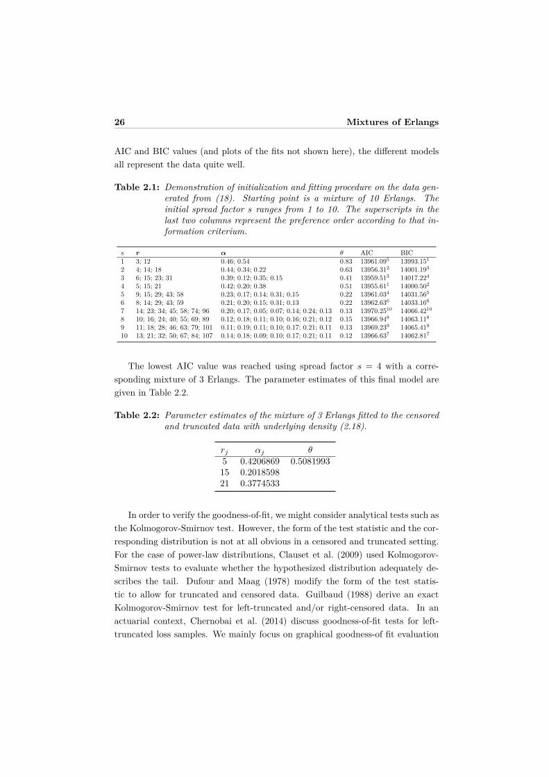
Table 2.1: Demonstration of initialization and fitting procedure on the data gen-erated from (18). Starting point is a mixture of 10 Erlangs. Theinitial spread factor s ranges from 1 to 10. The superscripts in thelast two columns represent the preference order according to that in-formation criterium.
s r α θ AIC BIC1 3; 12 0.46; 0.54 0.83 13961.095 13993.151
2 4; 14; 18 0.44; 0.34; 0.22 0.63 13956.312 14001.193
3 6; 15; 23; 31 0.39; 0.12; 0.35; 0.15 0.41 13959.513 14017.224
4 5; 15; 21 0.42; 0.20; 0.38 0.51 13955.611 14000.502
5 9; 15; 29; 43; 58 0.23; 0.17; 0.14; 0.31; 0.15 0.22 13961.034 14031.565
6 8; 14; 29; 43; 59 0.21; 0.20; 0.15; 0.31; 0.13 0.22 13962.636 14033.166
7 14; 23; 34; 45; 58; 74; 96 0.20; 0.17; 0.05; 0.07; 0.14; 0.24; 0.13 0.13 13970.2510 14066.4210
8 10; 16; 24; 40; 55; 69; 89 0.12; 0.18; 0.11; 0.10; 0.16; 0.21; 0.12 0.15 13966.948 14063.118
9 11; 18; 28; 46; 63; 79; 101 0.11; 0.19; 0.11; 0.10; 0.17; 0.21; 0.11 0.13 13969.239 14065.419
10 13; 21; 32; 50; 67; 84; 107 0.14; 0.18; 0.09; 0.10; 0.17; 0.21; 0.11 0.12 13966.637 14062.817
The lowest AIC value was reached using spread factor s = 4 with a corre-sponding mixture of 3 Erlangs. The parameter estimates of this final model aregiven in Table 2.2.
Table 2.2: Parameter estimates of the mixture of 3 Erlangs fitted to the censoredand truncated data with underlying density (2.18).
rj αj θ5 0.4206869 0.508199315 0.201859821 0.3774533
In order to verify the goodness-of-fit, we might consider analytical tests such asthe Kolmogorov-Smirnov test. However, the form of the test statistic and the cor-responding distribution is not at all obvious in a censored and truncated setting.For the case of power-law distributions, Clauset et al. (2009) used Kolmogorov-Smirnov tests to evaluate whether the hypothesized distribution adequately de-scribes the tail. Dufour and Maag (1978) modify the form of the test statis-tic to allow for truncated and censored data. Guilbaud (1988) derive an exactKolmogorov-Smirnov test for left-truncated and/or right-censored data. In anactuarial context, Chernobai et al. (2014) discuss goodness-of-fit tests for left-truncated loss samples. We mainly focus on graphical goodness-of fit evaluation
2.5. Examples 27
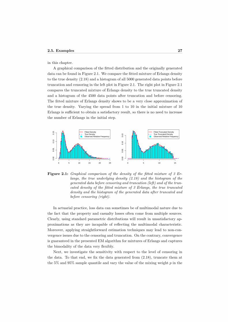
in this chapter.A graphical comparison of the fitted distribution and the originally generated
data can be found in Figure 2.1. We compare the fitted mixture of Erlangs densityto the true density (2.18) and a histogram of all 5000 generated data points beforetruncation and censoring in the left plot in Figure 2.1. The right plot in Figure 2.1compares the truncated mixture of Erlangs density to the true truncated densityand a histogram of the 4500 data points after truncation and before censoring.The fitted mixture of Erlangs density shows to be a very close approximation ofthe true density. Varying the spread from 1 to 10 in the initial mixture of 10Erlangs is sufficient to obtain a satisfactory result, so there is no need to increasethe number of Erlangs in the initial step.
0 5 10 15 20 25
0.00
0.05
0.10
0.15 Fitted Density
True DensityObserved Relative Frequency
0 5 10 15
0.00
0.05
0.10
0.15
Fitted Truncated DensityTrue Truncated DensityObserved Relative Frequency
Figure 2.1: Graphical comparison of the density of the fitted mixture of 3 Er-langs, the true underlying density (2.18) and the histogram of thegenerated data before censoring and truncation (left) and of the trun-cated density of the fitted mixture of 3 Erlangs, the true truncateddensity and the histogram of the generated data after truncated andbefore censoring (right).
In actuarial practice, loss data can sometimes be of multimodal nature due tothe fact that the property and casualty losses often come from multiple sources.Clearly, using standard parametric distributions will result in unsatisfactory ap-proximations as they are incapable of reflecting the multimodal characteristic.Moreover, applying straightforward estimation techniques may lead to non-con-vergence issues due to the censoring and truncation. On the contrary, convergenceis guaranteed in the presented EM algorithm for mixtures of Erlangs and capturesthe bimodality of the data very flexibly.
Next, we investigate the sensitivity with respect to the level of censoring inthe data. To that end, we fix the data generated from (2.18), truncate them atthe 5% and 95% sample quantile and vary the value of the mixing weight p in the
28 Mixtures of Erlangs
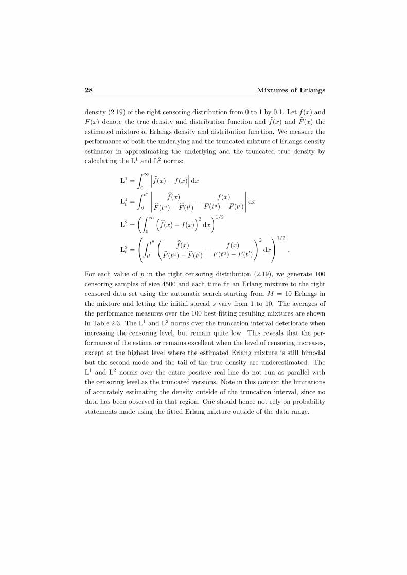
density (2.19) of the right censoring distribution from 0 to 1 by 0.1. Let f(x) andF (x) denote the true density and distribution function and f(x) and F (x) theestimated mixture of Erlangs density and distribution function. We measure theperformance of both the underlying and the truncated mixture of Erlangs densityestimator in approximating the underlying and the truncated true density bycalculating the L1 and L2 norms:
L1 =∫ ∞
0
∣∣∣f(x)− f(x)∣∣∣ dx
L1t =
∫ tu
tl
∣∣∣∣∣ f(x)F (tu)− F (tl)
− f(x)F (tu)− F (tl)
∣∣∣∣∣ dx
L2 =(∫ ∞
0
(f(x)− f(x)
)2dx
)1/2
L2t =
∫ tu
tl
(f(x)
F (tu)− F (tl)− f(x)
F (tu)− F (tl)
)2
dx
1/2
.
For each value of p in the right censoring distribution (2.19), we generate 100censoring samples of size 4500 and each time fit an Erlang mixture to the rightcensored data set using the automatic search starting from M = 10 Erlangs inthe mixture and letting the initial spread s vary from 1 to 10. The averages ofthe performance measures over the 100 best-fitting resulting mixtures are shownin Table 2.3. The L1 and L2 norms over the truncation interval deteriorate whenincreasing the censoring level, but remain quite low. This reveals that the per-formance of the estimator remains excellent when the level of censoring increases,except at the highest level where the estimated Erlang mixture is still bimodalbut the second mode and the tail of the true density are underestimated. TheL1 and L2 norms over the entire positive real line do not run as parallel withthe censoring level as the truncated versions. Note in this context the limitationsof accurately estimating the density outside of the truncation interval, since nodata has been observed in that region. One should hence not rely on probabilitystatements made using the fitted Erlang mixture outside of the data range.
2.5. Examples 29
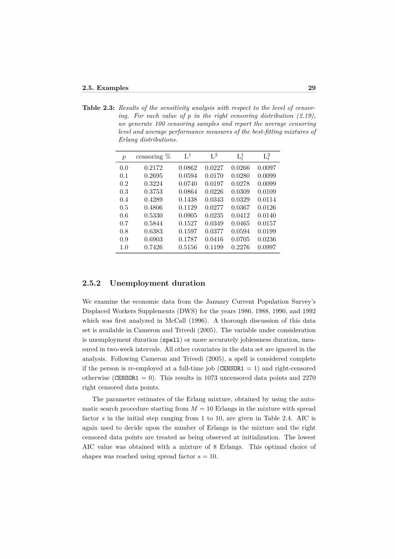
Table 2.3: Results of the sensitivity analysis with respect to the level of censor-ing. For each value of p in the right censoring distribution (2.19),we generate 100 censoring samples and report the average censoringlevel and average performance measures of the best-fitting mixtures ofErlang distributions.
p censoring % L1 L2 L1t L2
t
0.0 0.2172 0.0862 0.0227 0.0266 0.00970.1 0.2695 0.0594 0.0170 0.0280 0.00990.2 0.3224 0.0740 0.0197 0.0278 0.00990.3 0.3753 0.0864 0.0226 0.0309 0.01090.4 0.4289 0.1438 0.0343 0.0329 0.01140.5 0.4806 0.1129 0.0277 0.0367 0.01260.6 0.5330 0.0905 0.0235 0.0412 0.01400.7 0.5844 0.1527 0.0349 0.0465 0.01570.8 0.6383 0.1597 0.0377 0.0594 0.01990.9 0.6903 0.1787 0.0416 0.0705 0.02361.0 0.7426 0.5156 0.1199 0.2276 0.0997
2.5.2 Unemployment duration
We examine the economic data from the January Current Population Survey’sDisplaced Workers Supplements (DWS) for the years 1986, 1988, 1990, and 1992which was first analyzed in McCall (1996). A thorough discussion of this dataset is available in Cameron and Trivedi (2005). The variable under considerationis unemployment duration (spell) or more accurately joblessness duration, mea-sured in two-week intervals. All other covariates in the data set are ignored in theanalysis. Following Cameron and Trivedi (2005), a spell is considered completeif the person is re-employed at a full-time job (CENSOR1 = 1) and right-censoredotherwise (CENSOR1 = 0). This results in 1073 uncensored data points and 2270right censored data points.
The parameter estimates of the Erlang mixture, obtained by using the auto-matic search procedure starting from M = 10 Erlangs in the mixture with spreadfactor s in the initial step ranging from 1 to 10, are given in Table 2.4. AIC isagain used to decide upon the number of Erlangs in the mixture and the rightcensored data points are treated as being observed at initialization. The lowestAIC value was obtained with a mixture of 8 Erlangs. This optimal choice ofshapes was reached using spread factor s = 10.
30 Mixtures of Erlangs
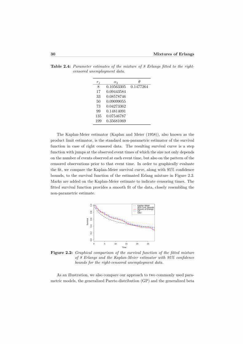
Table 2.4: Parameter estimates of the mixture of 8 Erlangs fitted to the right-censored unemployment data.
rj αj θ8 0.10563305 0.147726417 0.0944358433 0.0857874650 0.0909905573 0.0427336299 0.14814091135 0.07546787199 0.35681069
The Kaplan-Meier estimator (Kaplan and Meier (1958)), also known as theproduct limit estimator, is the standard non-parametric estimator of the survivalfunction in case of right censored data. The resulting survival curve is a stepfunction with jumps at the observed event times of which the size not only dependson the number of events observed at each event time, but also on the pattern of thecensored observations prior to that event time. In order to graphically evaluatethe fit, we compare the Kaplan-Meier survival curve, along with 95% confidencebounds, to the survival function of the estimated Erlang mixture in Figure 2.2.Marks are added on the Kaplan-Meier estimate to indicate censoring times. Thefitted survival function provides a smooth fit of the data, closely resembling thenon-parametric estimate.
0 5 10 15 20 25
0.0
0.2
0.4
0.6
0.8
1.0
Time
Sur
viva
l
Kaplan−Meier95% Conf. BoundsMixture of ErlangsGPGB2
Figure 2.2: Graphical comparison of the survival function of the fitted mixtureof 8 Erlangs and the Kaplan-Meier estimator with 95% confidencebounds for the right-censored unemployment data.
As an illustration, we also compare our approach to two commonly used para-metric models, the generalized Pareto distribution (GP) and the generalized beta

2.5. Examples 31
distribution of the second kind (GB2). In Figure 2.2, we see how mixtures ofErlangs offer much more flexibility and lead to a more appropriate fit for thesedata at the cost of requiring more parameters. However, AIC and BIC stronglyprefer the mixture of Erlangs approach, see Table 2.5.
Table 2.5: Comparison of information criteria for the different models fitted tothe right-censored unemployment data.
Model AIC BICMixtures of Erlangs 8066.281 8170.230Generalized Pareto (GP) 8733.718 8745.947Generalized beta 2 (GB2) 8280.168 8304.627
2.5.3 Secura Re, Belgian insurance data
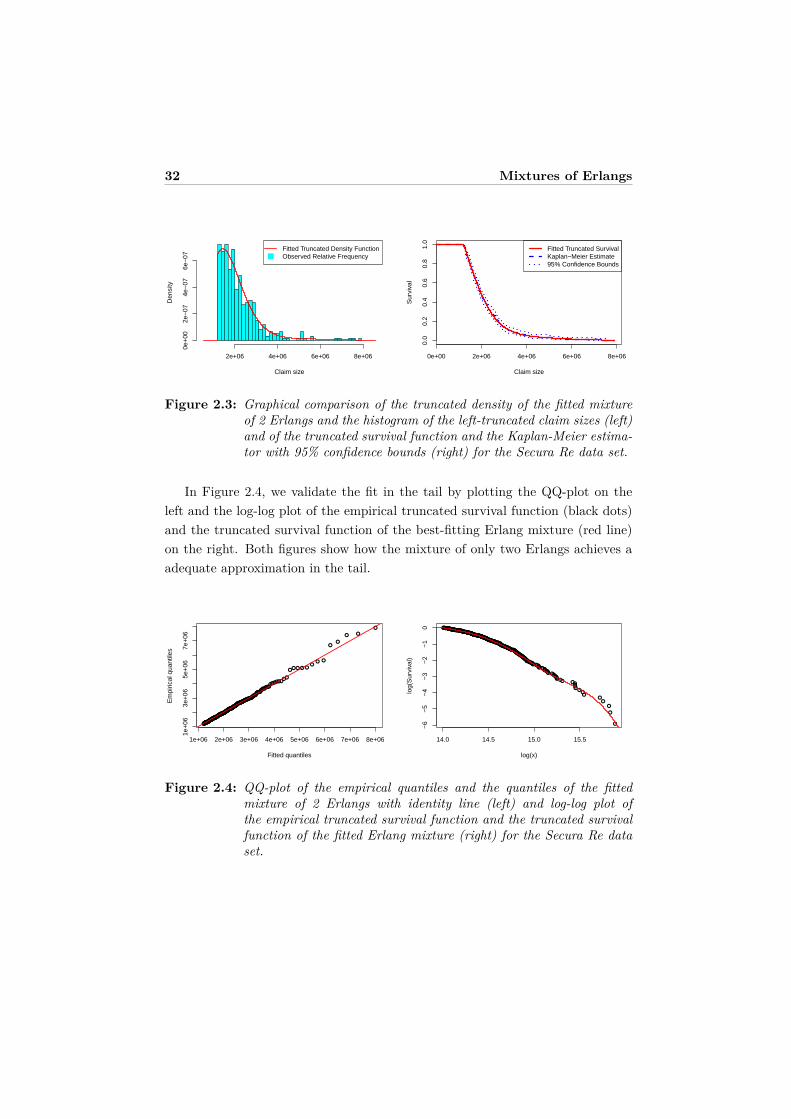
The Secura Re data set discussed in Beirlant et al. (2004) contains 371 automobileclaims from 1988 until 2001 gathered from several European insurance companies.The data are uncensored, but left truncated at 1 200 000 since a claim is onlyreported to the reinsurer if the claim size is at least as large as 1 200 000 euro.The sizes of the claims are corrected among others for inflation. Based on theseobservations, the reinsurer wants to calibrate a model in order to price reinsurancecontracts.
The search procedure using AIC prefers a mixture of only two Erlangs withshapes 5 and 16. The parameter estimates of this best-fitting mixture are shownin Table 2.6. In Figure 2.3 (left) we compare the histogram of the truncateddata to the fitted truncated density. Figure 2.3 (right) illustrates that the trun-cated survival function of the mixture of two Erlangs perfectly coincides with theKaplan-Meier estimate.
Table 2.6: Parameter estimates of the mixture of 2 Erlangs fitted to the left-truncated claim sizes in the Secura Re data set.
rj αj θ5 0.97103229 360 096.116 0.02896771
32 Mixtures of Erlangs
2e+06 4e+06 6e+06 8e+06
0e+
002e
−07
4e−
076e
−07
Claim size
Den
sity
Fitted Truncated Density FunctionObserved Relative Frequency
0e+00 2e+06 4e+06 6e+06 8e+06
0.0
0.2
0.4
0.6
0.8
1.0
Claim size
Sur
viva
l
Fitted Truncated SurvivalKaplan−Meier Estimate95% Confidence Bounds
Figure 2.3: Graphical comparison of the truncated density of the fitted mixtureof 2 Erlangs and the histogram of the left-truncated claim sizes (left)and of the truncated survival function and the Kaplan-Meier estima-tor with 95% confidence bounds (right) for the Secura Re data set.
In Figure 2.4, we validate the fit in the tail by plotting the QQ-plot on theleft and the log-log plot of the empirical truncated survival function (black dots)and the truncated survival function of the best-fitting Erlang mixture (red line)on the right. Both figures show how the mixture of only two Erlangs achieves aadequate approximation in the tail.
●●●●●●●●●●●●●●●●●●●●●●●●●●●●●●●●●●●●●●●●●●●●●●●●●●●●●●●●●●●●●●●●●●●●●
●●●●●●●●●●●●●●●●●●●●●●●●●●●●●●●●●●●●●●●●●●●●●●●●●●●●●●●●●●●●●●●●●●●●●●●●
●●●●●●●●●●●●●●●●●●●●●●●●●●●●●●●●●●●●●●●●●●●●●●●●●●●●●●●●●●●●●●●●●
●●●●●●●●●●●●●●●●●●●●●●●●●●●●●●●●●●●●●●●●●●●●●●
●●●●●●●●●●●●●●●●●●●●●●●●●●●
●●●●●●●●●●●●●●●●●●●●●●●●●●●●●●●●●●
●●●●●●●●●●●●●●●●●●●
●●●●●●●●
●●●●●●●●●
●●●●●●●
●●
●● ● ● ●●
● ●
●●
● ●
●
1e+06 2e+06 3e+06 4e+06 5e+06 6e+06 7e+06 8e+06
1e+
063e
+06
5e+
067e
+06
Fitted quantiles
Em
piric
al q
uant
iles
●●●●●●●●●●●●●●●●●●●●●●●●●●●●●●●●●●●●●●●●●●●●●●●●●●●●●●●●●●●●●●●●●●●●●●●●●●●●●●●●●●●●●●●●●●●●●●●●●●●●●●●●●●●●●●●●●●●●●●●●●●●●●●●●●●●●●●●●●●●●●●●●●●●●●●●●●●●●●●●●●●●●●●●●●●●●●●●●●●●●●●●●●●●●●●●●●●●●●●●●●●●●●●●●●●●●●●●●●●●●●●●●●●●●●●●●●●●●●●●●●●●●●●●●●●●●●●●●●●●●●●●●●●●●●●●●●●●●●●●●●●●●●●●●●●●●●●●●●●●●●●●●●●●●●●●●●●●●●●●●●●●●●●●●●●●●●●●●●●●●●●●●●●●●●●●●●●●●●● ●●●●●●●●
●●
●
●
●
14.0 14.5 15.0 15.5
−6
−5
−4
−3
−2
−1
0
log(x)
log(
Sur
viva
l)
Figure 2.4: QQ-plot of the empirical quantiles and the quantiles of the fittedmixture of 2 Erlangs with identity line (left) and log-log plot ofthe empirical truncated survival function and the truncated survivalfunction of the fitted Erlang mixture (right) for the Secura Re dataset.
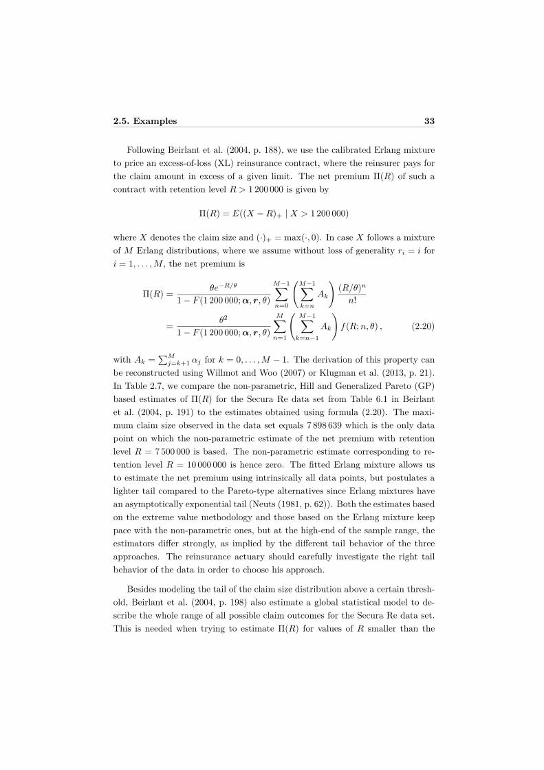
2.5. Examples 33
Following Beirlant et al. (2004, p. 188), we use the calibrated Erlang mixtureto price an excess-of-loss (XL) reinsurance contract, where the reinsurer pays forthe claim amount in excess of a given limit. The net premium Π(R) of such acontract with retention level R > 1 200 000 is given by
Π(R) = E((X −R)+ | X > 1 200 000)
where X denotes the claim size and (·)+ = max(·, 0). In case X follows a mixtureof M Erlang distributions, where we assume without loss of generality ri = i fori = 1, . . . , M , the net premium is
Π(R) = θe−R/θ
1− F (1 200 000;α, r, θ)
M−1∑n=0
(M−1∑k=n
Ak
)(R/θ)n
n!
= θ2
1− F (1 200 000;α, r, θ)
M∑n=1
(M−1∑
k=n−1Ak
)f(R; n, θ) , (2.20)
with Ak =∑M
j=k+1 αj for k = 0, . . . , M − 1. The derivation of this property canbe reconstructed using Willmot and Woo (2007) or Klugman et al. (2013, p. 21).In Table 2.7, we compare the non-parametric, Hill and Generalized Pareto (GP)based estimates of Π(R) for the Secura Re data set from Table 6.1 in Beirlantet al. (2004, p. 191) to the estimates obtained using formula (2.20). The maxi-mum claim size observed in the data set equals 7 898 639 which is the only datapoint on which the non-parametric estimate of the net premium with retentionlevel R = 7 500 000 is based. The non-parametric estimate corresponding to re-tention level R = 10 000 000 is hence zero. The fitted Erlang mixture allows usto estimate the net premium using intrinsically all data points, but postulates alighter tail compared to the Pareto-type alternatives since Erlang mixtures havean asymptotically exponential tail (Neuts (1981, p. 62)). Both the estimates basedon the extreme value methodology and those based on the Erlang mixture keeppace with the non-parametric ones, but at the high-end of the sample range, theestimators differ strongly, as implied by the different tail behavior of the threeapproaches. The reinsurance actuary should carefully investigate the right tailbehavior of the data in order to choose his approach.
Besides modeling the tail of the claim size distribution above a certain thresh-old, Beirlant et al. (2004, p. 198) also estimate a global statistical model to de-scribe the whole range of all possible claim outcomes for the Secura Re data set.This is needed when trying to estimate Π(R) for values of R smaller than the
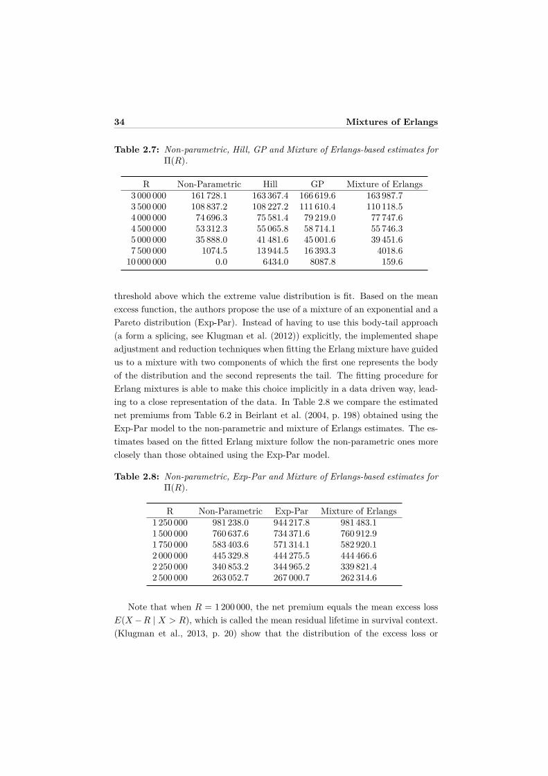
34 Mixtures of Erlangs
Table 2.7: Non-parametric, Hill, GP and Mixture of Erlangs-based estimates forΠ(R).
R Non-Parametric Hill GP Mixture of Erlangs3 000 000 161 728.1 163 367.4 166 619.6 163 987.73 500 000 108 837.2 108 227.2 111 610.4 110 118.54 000 000 74 696.3 75 581.4 79 219.0 77 747.64 500 000 53 312.3 55 065.8 58 714.1 55 746.35 000 000 35 888.0 41 481.6 45 001.6 39 451.67 500 000 1074.5 13 944.5 16 393.3 4018.6
10 000 000 0.0 6434.0 8087.8 159.6
threshold above which the extreme value distribution is fit. Based on the meanexcess function, the authors propose the use of a mixture of an exponential and aPareto distribution (Exp-Par). Instead of having to use this body-tail approach(a form a splicing, see Klugman et al. (2012)) explicitly, the implemented shapeadjustment and reduction techniques when fitting the Erlang mixture have guidedus to a mixture with two components of which the first one represents the bodyof the distribution and the second represents the tail. The fitting procedure forErlang mixtures is able to make this choice implicitly in a data driven way, lead-ing to a close representation of the data. In Table 2.8 we compare the estimatednet premiums from Table 6.2 in Beirlant et al. (2004, p. 198) obtained using theExp-Par model to the non-parametric and mixture of Erlangs estimates. The es-timates based on the fitted Erlang mixture follow the non-parametric ones moreclosely than those obtained using the Exp-Par model.
Table 2.8: Non-parametric, Exp-Par and Mixture of Erlangs-based estimates forΠ(R).
R Non-Parametric Exp-Par Mixture of Erlangs1 250 000 981 238.0 944 217.8 981 483.11 500 000 760 637.6 734 371.6 760 912.91 750 000 583 403.6 571 314.1 582 920.12 000 000 445 329.8 444 275.5 444 466.62 250 000 340 853.2 344 965.2 339 821.42 500 000 263 052.7 267 000.7 262 314.6
Note that when R = 1 200 000, the net premium equals the mean excess lossE(X −R | X > R), which is called the mean residual lifetime in survival context.(Klugman et al., 2013, p. 20) show that the distribution of the excess loss or
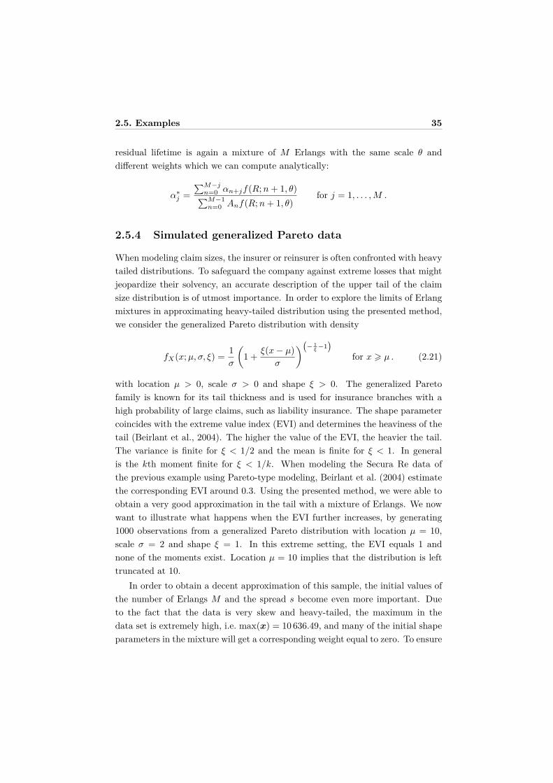
2.5. Examples 35
residual lifetime is again a mixture of M Erlangs with the same scale θ anddifferent weights which we can compute analytically:
α∗j =
∑M−jn=0 αn+jf(R; n + 1, θ)∑M−1
n=0 Anf(R; n + 1, θ)for j = 1, . . . , M .
2.5.4 Simulated generalized Pareto data
When modeling claim sizes, the insurer or reinsurer is often confronted with heavytailed distributions. To safeguard the company against extreme losses that mightjeopardize their solvency, an accurate description of the upper tail of the claimsize distribution is of utmost importance. In order to explore the limits of Erlangmixtures in approximating heavy-tailed distribution using the presented method,we consider the generalized Pareto distribution with density
fX(x; µ, σ, ξ) = 1σ
(1 + ξ(x− µ)
σ
)(− 1ξ −1)
for x > µ . (2.21)
with location µ > 0, scale σ > 0 and shape ξ > 0. The generalized Paretofamily is known for its tail thickness and is used for insurance branches with ahigh probability of large claims, such as liability insurance. The shape parametercoincides with the extreme value index (EVI) and determines the heaviness of thetail (Beirlant et al., 2004). The higher the value of the EVI, the heavier the tail.The variance is finite for ξ < 1/2 and the mean is finite for ξ < 1. In generalis the kth moment finite for ξ < 1/k. When modeling the Secura Re data ofthe previous example using Pareto-type modeling, Beirlant et al. (2004) estimatethe corresponding EVI around 0.3. Using the presented method, we were able toobtain a very good approximation in the tail with a mixture of Erlangs. We nowwant to illustrate what happens when the EVI further increases, by generating1000 observations from a generalized Pareto distribution with location µ = 10,scale σ = 2 and shape ξ = 1. In this extreme setting, the EVI equals 1 andnone of the moments exist. Location µ = 10 implies that the distribution is lefttruncated at 10.
In order to obtain a decent approximation of this sample, the initial values ofthe number of Erlangs M and the spread s become even more important. Dueto the fact that the data is very skew and heavy-tailed, the maximum in thedata set is extremely high, i.e. max(x) = 10 636.49, and many of the initial shapeparameters in the mixture will get a corresponding weight equal to zero. To ensure
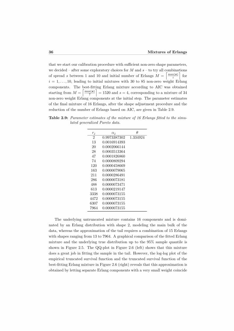
36 Mixtures of Erlangs
that we start our calibration procedure with sufficient non-zero shape parameters,we decided – after some exploratory choices for M and s – to try all combinationsof spread s between 1 and 10 and initial number of Erlangs M =
⌈max(x)
i
⌉for
i = 1, . . . , 10, leading to initial mixtures with 30 to 85 non-zero weight Erlangcomponents. The best-fitting Erlang mixture according to AIC was obtainedstarting from M =
⌈max(x)
7
⌉= 1520 and s = 4, corresponding to a mixture of 34
non-zero weight Erlang components at the initial step. The parameter estimatesof the final mixture of 16 Erlangs, after the shape adjustment procedure and thereduction of the number of Erlangs based on AIC, are given in Table 2.9.
Table 2.9: Parameter estimates of the mixture of 16 Erlangs fitted to the simu-lated generalized Pareto data.
rj αj θ2 0.9973387302 1.33492413 0.001691439320 0.000206614428 0.000351336447 0.000182686074 0.0000809294120 0.0000458669163 0.0000079065211 0.0000286491286 0.0000073181488 0.0000073471613 0.00002191473338 0.00000731554472 0.00000731556307 0.00000731557964 0.0000073155
The underlying untruncated mixture contains 16 components and is domi-nated by an Erlang distribution with shape 2, modeling the main bulk of thedata, whereas the approximation of the tail requires a combination of 15 Erlangswith shapes ranging from 13 to 7964. A graphical comparison of the fitted Erlangmixture and the underlying true distribution up to the 95% sample quantile isshown in Figure 2.5. The QQ-plot in Figure 2.6 (left) shows that this mixturedoes a great job in fitting the sample in the tail. However, the log-log plot of theempirical truncated survival function and the truncated survival function of thebest-fitting Erlang mixture in Figure 2.6 (right) reveals that this approximation isobtained by letting separate Erlang components with a very small weight coincide
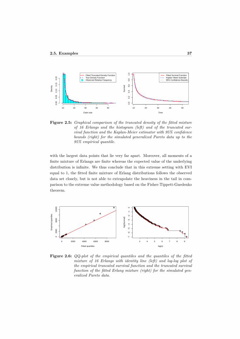
2.5. Examples 37
10 20 30 40 50
0.00
0.05
0.10
0.15
0.20
Claim size
Den
sity
Fitted Truncated Density FunctionTrue Density FunctionObserved Relative Frequency
10 20 30 40 50
0.0
0.2
0.4
0.6
0.8
1.0
Time
Sur
viva
l
Fitted Survival FunctionKaplan−Meier Estimate95% Confidence Bounds
Figure 2.5: Graphical comparison of the truncated density of the fitted mixtureof 16 Erlangs and the histogram (left) and of the truncated sur-vival function and the Kaplan-Meier estimator with 95% confidencebounds (right) for the simulated generalized Pareto data up to the95% empirical quantile.
with the largest data points that lie very far apart. Moreover, all moments of afinite mixture of Erlangs are finite whereas the expected value of the underlyingdistribution is infinite. We thus conclude that in this extreme setting with EVIequal to 1, the fitted finite mixture of Erlang distributions follows the observeddata set closely, but is not able to extrapolate the heaviness in the tail in com-parison to the extreme value methodology based on the Fisher-Tippett-Gnedenkotheorem.
●●●●●●●●●●●●●●●●●●●●●●●●●●●●●●●●●●●●●●●●●●●●●●●●●●●●●●●●●●●●●●●●●●●●●●●●●●●●●●●●●●●●●●●●●●●●●●●●●●●●●●●●●●●●●●●●●●●●●●●●●●●●●●●●●●●●●●●●●●●●●●●●●●●●●●●●●●●●●●●●●●●●●●●●●●●●●●●●●●●●●●●●●●●●●●●●●●●●●●●●●●●●●●●●●●●●●●●●●●●●●●●●●●●●●●●●●●●●●●●●●●●●●●●●●●●●●●●●●●●●●●●●●●●●●●●●●●●●●●●●●●●●●●●●●●●●●●●●●●●●●●●●●●●●●●●●●●●●●●●●●●●●●●●●●●●●●●●●●●●●●●●●●●●●●●●●●●●●●●●●●●●●●●●●●●●●●●●●●●●●●●●●●●●●●●●●●●●●●●●●●●●●●●●●●●●●●●●●●●●●●●●●●●●●●●●●●●●●●●●●●●●●●●●●●●●●●●●●●●●●●●●●●●●●●●●●●●●●●●●●●●●●●●●●●●●●●●●●●●●●●●●●●●●●●●●●●●●●●●●●●●●●●●●●●●●●●●●●●●●●●●●●●●●●●●●●●●●●●●●●●●●●●●●●●●●●●●●●●●●●●●●●●●●●●●●●●●●●●●●●●●●●●●●●●●●●●●●●●●●●●●●●●●●●●●●●●●●●●●●●●●●●●●●●●●●●●●●●●●●●●●●●●●●●●●●●●●●●●●●●●●●●●●●●●●●●●●●●●●●●●●●●●●●●●●●●●●●●●●●●●●●●●●●●●●●●●●●●●●●●●●●●●●●●●●●●●●●●●●●●●●●●●●●●●●●●●●●●●●●●●●●●●●●●●●●●●●●●●●●●●●●●●●●●●●●●●●●●●●●●●●●●●●●●●●●●●●●●●●●●●●●●●●●●●●●●●●●●●●●●●●●●●●●●●●●●●●●●●●●●●●●●●●●●●●●●●●●●●●●●●●●●●●●●●●●●●●●●●●●●●●●●●●●●●●●●●●●●●●●●●●●●●●●●●●●●●●●●●●●●●●●●●●●●●●●●●●●●●●●●●●●●●●●●●●●●
●●●●
●
●
●
●
0 2000 4000 6000 8000
020
0060
0010
000
Fitted quantiles
Em
piric
al q
uant
iles
●●●●●●●●●●●●●●●●●●●●●●●●●●●●●●●●●●●●●●●●●●●●●●●●●●●●●●●●●●●●●●●●●●●●●●●●●●●●●●●●●●●●●●●●●●●●●●●●●●●●●●●●●●●●●●●●●●●●●●●●●●●●●●●●●●●●●●●●●●●●●●●●●●●●●●●●●●●●●●●●●●●●●●●●●●●●●●●●●●●●●●●●●●●●●●●●●●●●●●●●●●●●●●●●●●●●●●●●●●●●●●●●●●●●●●●●●●●●●●●●●●●●●●●●●●●●●●●●●●●●●●●●●●●●●●●●●●●●●●●●●●●●●●●●●●●●●●●●●●●●●●●●●●●●●●●●●●●●●●●●●●●●●●●●●●●●●●●●●●●●●●●●●●●●●●●●●●●●●●●●●●●●●●●●●●●●●●●●●●●●●●●●●●●●●●●●●●●●●●●●●●●●●●●●●●●●●●●●●●●●●●●●●●●●●●●●●●●●●●●●●●●●●●●●●●●●●●●●●●●●●●●●●●●●●●●●●●●●●●●●●●●●●●●●●●●●●●●●●●●●●●●●●●●●●●●●●●●●●●●●●●●●●●●●●●●●●●●●●●●●●●●●●●●●●●●●●●●●●●●●●●●●●●●●●●●●●●●●●●●●●●●●●●●●●●●●●●●●●●●●●●●●●●●●●●●●●●●●●●●●●●●●●●●●●●●●●●●●●●●●●●●●●●●●●●●●●●●●●●●●●●●●●●●●●●●●●●●●●●●●●●●●●●●●●●●●●●●●●●●●●●●●●●●●●●●●●●●●●●●●●●●●●●●●●●●●●●●●●●●●●●●●●●●●●●●●●●●●●●●●●●●●●●●●●●●●●●●●●●●●●●●●●●●●●●●●●●●●●●●●●●●●●●●●●●●●●●●●●●●●●●●●●●●●●●●●●●●●●●●●●●●●●●●●●●●●●●●●●●●●●●●●●●●●●●●●●●●●●●●●●●●●●●●●●●●●●●●●●●●●●●●●●●●●●●●●●●●●●●●●●●●●●●●●●●●●●●●●●●●●●●●●●●●●●●●●●●●●●●●●●●●●●●●●●●●●●●●●●●●● ●●●●●● ● ●●●● ● ●●●●
●●
●
●
3 4 5 6 7 8 9
−7
−6
−5
−4
−3
−2
−1
0
log(x)
log(
Sur
viva
l)
Figure 2.6: QQ-plot of the empirical quantiles and the quantiles of the fittedmixture of 16 Erlangs with identity line (left) and log-log plot ofthe empirical truncated survival function and the truncated survivalfunction of the fitted Erlang mixture (right) for the simulated gen-eralized Pareto data.
38 Mixtures of Erlangs
2.6 Discussion
We extend the Lee and Lin (2010) EM algorithm for fitting mixtures of Erlangswith a common scale parameter to censored and truncated data. The EM algo-rithm able to deal with censored and truncated data remains a simple iterativealgorithm. The initialization of the parameters can be done in a similar way asin Lee and Lin (2010) based on the denseness property (Tijms, 1994, p. 163) andprovides close starting values making the algorithm converge fast. The shape ad-justment procedure explores the parameter space in a clever way such that, whenadjusting and reducing the shapes, the previous estimates for the scale and theweights provide a very close approximation to the maximum likelihood estimatescorresponding to the new set of shapes, which greatly reduces the run time. Ex-tending Lee and Lin (2010), we suggest the use of a spread factor to achieve awider spread for the shapes at the initial step. We recommend comparing theresulting fits starting from different initial values obtained by varying the spreadfactor and changing the initial number of Erlangs.
We implement the fitting procedure in R and show how mixtures of Erlangscan be used to adequately represent any univariate distribution in a wide varietyof applications where data is allowed to be censored and truncated. We focus onthe domain of actuarial science, where claim severity data is often censored andtruncated due to policy modifications such as deductibles and policy limits. Theuse of mixtures of Erlangs offers on the one hand the flexibility of nonparametricdensity estimation techniques to describe the insurance losses and on the otherhand the feasibility to analytically quantify the risk. The examples on severalsimulated and real data sets illustrate the effectiveness of our proposed algorithmand demonstrate the approximation strength of mixtures of Erlangs.
Future research may explore incorporating regressor variables in the mixtureof Erlangs with common scale and introducing the flexibility of this approachin a regression context. We detected some limitations of mixtures of Erlangs inapproximating heavy-tailed distributions and suggest combining our methodologywith the extreme value methodology using a body-tail approach (Lee et al., 2012;Pigeon and Denuit, 2011). Adjusting the EM algorithm tailored to the class ofmultivariate mixtures of Erlangs, introduced by Lee and Lin (2012), to the caseof censored and truncated data is another appealing extension.

2.7. Appendix A: Denseness 39
2.7 Appendix A: Denseness
Theorem 2.7.1. (Tijms, 1994, p. 163) The class of mixtures of Erlang distri-butions with a common scale parameter is dense in the space of distributions onR+. More specifically, let G(x) be the cumulative distribution function of a pos-itive random variable. Define the following cumulative distribution function of amixture of Erlang distributions with a common scale parameter θ > 0,
F (x; θ) =∞∑
j=1αj(θ)F (x; j, θ) ,
where F (x; j, θ) denotes the cumulative distribution function of an Erlang distri-bution with shape j and scale θ,
F (x; j, θ) = 1−j−1∑n=0
e−x/θ (x/θ)n
n! ,
and the mixing weights are given by
αj(θ) = G(jθ)−G((j − 1)θ) for j = 1, 2, . . . .
Thenlimθ→0
F (x; θ) = G(x) ,
for each point x at which G(·) is continuous.
2.8 Appendix B: Partial derivative of Q
We first introduce the lower incomplete gamma function
γ(s, x) =∫ x
0zs−1e−zdz ,
by which we can write the cumulative distribution function of an Erlang distri-bution as
F (x; r, θ) =∫ x
0
zr−1e−z/θ
θr(r − 1)! dz = 1(r − 1)!
∫ x/θ
0ur−1e−udu = γ(r, x/θ)
(r − 1)! . (2.22)
40 Mixtures of Erlangs
In order to maximize Q(Θ; Θ(k−1)) with respect to θ, we set the first order partialderivative at θ(k) equal to zero
∂Q(Θ; Θ(k−1))∂θ
∣∣∣∣∣θ=θ(k)
=∑i∈U
M∑j=1
uz(k)ij
(xi
θ2 −rj
θ−
∂∂θ
[F (tu; rj , θ)− F (tl; rj , θ)
]F (tu; rj , θ)− F (tl; rj , θ)
)
+∑i∈C
M∑j=1
cz(k)ij
(E(Xi
∣∣Zij = 1, li, ui, tl, tu; θ(k−1) )θ2 − rj
θ
−∂
∂θ
[F (tu; rj , θ)− F (tl; rj , θ)
]F (tu; rj , θ)− F (tl; rj , θ)
)∣∣∣∣∣θ=θ(k)
(2.22)= 1θ2
∑i∈U
M∑j=1
uz(k)ij
xi
+ 1θ2
∑i∈C
M∑j=1
cz(k)ij E
(Xi
∣∣∣Zij = 1, li, ui, tl, tu; θ(k−1))
−n
θ
M∑j=1
(∑i∈U
uz(k)ij +
∑i∈C
cz(k)ij
n
)rj
−∑i∈U
M∑j=1
uz(k)ij
∂∂θ
(γ(rj , tu/θ)− γ(rj , tl/θ)
)(rj − 1)! (F (tu; rj , θ)− F (tl; rj , θ))
−∑i∈C
M∑j=1
cz(k)ij
∂∂θ
(γ(rj , tu/θ)− γ(rj , tl/θ)
)(rj − 1)! (F (tu; rj , θ)− F (tl; rj , θ))
∣∣∣∣∣∣θ=θ(k)
(2.16)= 1θ2
∑i∈U
xi + 1θ2
∑i∈C
E(
Xi
∣∣∣li, ui, tl, tu; θ(k−1))− n
θ
M∑j=1
β(k)j rj
−∑i∈U
M∑j=1
uz(k)ij
tl/θ2 (tl/θ)rj−1
e−tl/θ − tu/θ2 (tu/θ)rj−1e−tu/θ
(rj − 1)! (F (tu; rj , θ)− F (tl; rj , θ))
−∑i∈C
M∑j=1
cz(k)ij
tl/θ2 (tl/θ)rj−1
e−tl/θ − tu/θ2 (tu/θ)rj−1e−tu/θ
(rj − 1)! (F (tu; rj , θ)− F (tl; rj , θ))
∣∣∣∣∣∣θ=θ(k)
= 1θ2
∑i∈U
xi + 1θ2
∑i∈C
E(
Xi
∣∣∣li, ui, tl, tu; θ(k−1))− n
θ
M∑j=1
β(k)j rj

2.8. Appendix B: Partial derivative of Q 41
− n
θ2
M∑j=1
β(k)j
(tl)rj
e−tl/θ − (tu)rj e−tu/θ
θrj−1(rj − 1)! (F (tu; rj , θ)− F (tl; rj , θ))
∣∣∣∣∣∣θ=θ(k)
= 0 ,
where we used expression (2.22) of the cumulative distribution of an Erlang.

Chapter 3
Multivariate mixtures of Erlangs
for density estimation under
censoring
Abstract
Multivariate mixtures of Erlang distributions form a versatile, yet analyti-cally tractable, class of distributions making them suitable for multivariatedensity estimation. We present a flexible and effective fitting procedurefor multivariate mixtures of Erlangs, which iteratively uses the EM algo-rithm, by introducing a computationally efficient initialization and adjust-ment strategy for the shape parameter vectors. We furthermore extend theEM algorithm for multivariate mixtures of Erlangs to be able to deal withrandomly censored and fixed truncated data. The effectiveness of the pro-posed algorithm is demonstrated on simulated as well as real data sets.
This chapter is based on Verbelen, R., Antonio, K., and Claeskens, G. (2016).Multivariate mixtures of Erlangs for density estimation under censoring. LifetimeData Analysis, 22(3):429-455.
3.1 Introduction
We present an estimation technique for fitting multivariate mixtures of Erlangdistributions (MME). We suggest an efficient initialization method and adjust-
43
44 Multivariate mixtures of Erlangs
ment strategy for the values of the shape parameter vectors of an MME, whichhas been underexposed in the literature. The fitting procedure is also extendedto take random censoring and fixed truncation into account. Data are censored incase you only observe an interval in which a data point is lying without knowingits exact value. Truncation entails that it is only possible to observe the data ofwhich the values lie in a certain range. Censoring and/or truncation is often thecase in applications such as loss modeling (finance and actuarial science), clini-cal experiments (survival/failure time analysis), veterinary studies (e.g. mastitisstudies), and duration data (econometric studies).
The class of MME is introduced by Lee and Lin (2012). MME form a highlyflexible class of distributions as they are dense in the space of positive continu-ous multivariate distributions in the sense of weak convergence, extending thisproperty of the univariate class (Tijms, 1994). An overview of the analytical anddistributional properties of mixtures of Erlangs can be found in Klugman et al.(2013), Willmot and Lin (2011) and Willmot and Woo (2007). Parameter esti-mation in the univariate case is treated in Lee and Lin (2010) and extended to beable to deal with randomly censored and fixed truncated data in Verbelen et al.(2015).
Mixtures of Erlangs have received most attention in the field of actuarial sci-ence. Cossette et al. (2013a) model the joint distribution of a portfolio of de-pendent risks using univariate mixtures of Erlangs as marginals along with theFarlie-Gumbel-Morgenstern (FGM) copula. Cossette et al. (2013b) and Mailhot(2012) study the bivariate lower and upper orthant Value-at-Risk and use MMEas an illustration. Willmot and Woo (2015) study the analytical properties of theMME class. They motivate the use of MME in actuarial science and illustratehow their tractability leads to closed-form expressions.
The use of MME should be regarded as a multivariate density estimationtechnique, not as a type of model-based clustering. The MME model can beseen as semiparametric, since the mixture components have a specific parametricform, whereas the mixing weights can have a nonparametric nature, and is aninteresting alternative to the use of copulas, which is the dominant choice to modelmultivariate data in a two stage procedure, separating the dependence structurefrom the marginal distributions (see e.g. Joe, 1997; Nelsen, 2006). In contrast,MME are able to model the multivariate data directly on the original scale. TheMME model enjoys many desirable properties of a multivariate model as listedby Joe (1997, p. 84), see Lee and Lin (2012), with regard to interpretability,closure, flexibility and wide range of dependence, and closed-form representation,
3.1. Introduction 45
often not satisfied for the commonly used copula structures. Lee and Lin (2012)demonstrate the flexibility of MME by fitting 12-dimensional data generated froma multivariate lognormal distribution and extremely dependent bivariate datawith Spearman’s rho very close to 1 or −1.
An extensive literature exists on mixtures of multivariate normals (see e.g.McLachlan and Peel, 2001). Lee and Scott (2012) discuss the estimation of mul-tivariate Gaussian mixtures in case the data can be randomly censored and fixedtruncated. Due to the limitations of Gaussian mixtures, such as the difficultyin modeling skewed data, non-Gaussian approaches have received an increasinginterest over the last years. Important examples include mixtures of multivari-ate t-distributions (see e.g. Peel and McLachlan, 2000), mixtures of multivariateskew-normal distributions (see e.g. Lin, 2009), and mixtures of multivariate skew-tdistributions (see e.g. Lee and McLachlan, 2014). All of these mixture models in-volve modeling real-valued multivariate random variables, whereas in this chapterwe consider multivariate positive-valued random variables.
Lee and Lin (2012) show in Theorem 2.3 that a finite multivariate Erlangmixture is a multivariate phase-type distribution, a generalization of the class ofunivariate phase-type distributions introduced by Assaf et al. (1984). Parameterestimation for phase-type distributions in the bivariate case (Eisele, 2005; Zadehand Bilodeau, 2013), as in the univariate case (Asmussen et al., 1996; Olsson,1996), uses the expectation-maximization (EM) algorithm, first introduced byDempster et al. (1977)
The EM algorithm forms the key to fit an MME to multivariate positive data.Taking censoring and truncation into account when calibrating data using copu-las is cumbersome, especially in more than two dimensions, due to complicatedforms of the likelihood (see e.g. Georges et al., 2001) which are hard to optimizenumerically. This is, as we will show, not the case for the MME class due tothe EM algorithm. As opposed to the traditional way of dealing with groupedand truncated data using the EM algorithm (Dempster et al., 1977; McLachlanand Krishnan, 2008, p. 66; McLachlan and Peel, 2001, p. 257; McLachlan andJones, 1988), we follow the approach of Lee and Scott (2012), as was done in theunivariate setting (Verbelen et al., 2015).
We demonstrate the effectiveness of our proposed algorithm and the practicaluse of MME on a simulated data set, the old faithful geyser data and a four-dimensional data set of interval and right censored udder quarter infection times,each time highlighting one of the analytical aspects of MME.
46 Multivariate mixtures of Erlangs
3.2 Multivariate Erlang mixtures with a commonscale parameter
In this section, we briefly revise the definition of a multivariate mixture of Er-lang distributions with a common scale parameter and the denseness property ofthis distributional class. These formulas are extended in Section 3.3.1 and 3.3.2towards censoring and truncation.
The Erlang distribution is a positive continuous distribution with density func-tion
f(x; r, θ) = xr−1e−x/θ
θr(r − 1)! for x > 0 , (3.1)
where r, a positive integer, is the shape parameter and θ > 0 the scale parameter(the inverse λ = 1/θ is called the rate parameter). The cumulative distributionfunction is obtained by integrating (3.1) by parts r times
F (x; r, θ) = 1−r−1∑n=0
e−x/θ (x/θ)n
n! = γ(r, x/θ)(r − 1)! , (3.2)
using the lower incomplete gamma function defined as γ(s, x) =∫ x
0 zs−1e−zdz.A univariate Erlang distribution is in fact a gamma distribution of which the
shape parameter is a positive integer and can therefore be seen as the distributionof a sum of i.i.d. exponential random variables. Lee and Lin (2012) define a d-variate Erlang mixture as a mixture such that each mixture component is thejoint distribution of d independent Erlang distributions with a common scaleparameter θ > 0. The dependence structure is captured by the combinationof the positive integer shape parameters of the Erlangs in each dimension. Wedenote the positive integer shape parameters of the jointly independent Erlangdistributions in a mixture component by the vector r = (r1, . . . , rd) and the set ofall shape vectors with non-zero weight by R. The mixture weights are denoted byα = {αr |r ∈ R} and must satisfy αr > 0 and
∑r∈R αr = 1. The density of a d-
variate Erlang mixture evaluated in x = (x1, . . . , xd) with xj > 0 for j = 1, . . . , d
can then be written as
f(x;α, r, θ) =∑r∈R
αrf(x; r, θ) =∑r∈R
αr
d∏j=1
f(xj ; rj , θ)
=∑r∈R
αr
d∏j=1
xrj−1j e−xj/θ
θrj (rj − 1)! . (3.3)
3.2. Multivariate Erlang mixtures with a common scale parameter 47
The following property states that for any positive multivariate distributionthere exists a sequence of multivariate Erlang distributions that weakly convergesto the target distribution. The proof is given in the appendix of Lee and Lin(2012).
Property 1 (Lee and Lin 2012). The class of multivariate Erlang mixtures ofform (3.3) is dense in the space of positive continuous multivariate distributionsin the sense of weak convergence. More specifically, let g(x) be the density func-tion of a d-variate positive random variable with cumulative distribution functionG(x). For any given θ > 0, define the following d-variate Erlang mixture
f(x; θ) =∞∑
r1=1· · ·
∞∑rd=1
αr(θ)d∏
j=1f(xj ; rj , θ) , (3.4)
with mixing weights
αr(θ) =∫ r1θ
(r1−1)θ
· · ·∫ rdθ
(rd−1)θ
g(x)dx . (3.5)
Then limθ→0
F (x; θ) = G(x) for each point x at which F is continuous.
In Property 1, for any given common scale θ > 0, an infinite multivariatemixture of Erlangs in (3.4) is considered using combinations of shapes from 1to infinity in each marginal dimension. The weights in (3.5) of the componentsin the mixture are defined by integrating the density over the corresponding d-dimensional rectangle of the d-dimensional grid formed by the shape parame-ters multiplied with the common scale. When the value of the common scale θ
decreases, this grid becomes more refined and the sequence of Erlang mixturesconverges to the underlying cumulative distribution function.
Next to its flexibility, Lee and Lin (2012) show that it is easy to work ana-lytically with this class of distributions due to the independence structure of theErlang distributions within each mixture component. This leads to explicit ex-pressions of many distributional quantities such as the characteristic function, thejoint moments and bivariate measures of association (Kendall’s tau and Spear-man’s rho). The authors further reveal interesting closure properties, such asthe fact that each p-variate marginal or conditional distribution with p 6 d canagain be written as a p-variate Erlang distribution. The same property holds forthe distribution of the multivariate excess losses (actuarial science context) ormultivariate residual lifetimes (survival analysis context). Furthermore, the dis-
48 Multivariate mixtures of Erlangs
tribution of the sum of the component random variables of an MME distributedrandom variable is a univariate Erlang mixture distribution.
Willmot and Woo (2015) consider an extension of the MME class, allowingdifferent scale parameters in each dimension. However, in Proposition 1 they showhow a multivariate mixture of Erlangs distribution with different scale parameterscan be rewritten as a multivariate mixture of Erlangs distribution with a commonscale parameter, which is smaller than all original scales. We thus concentrate onmodels with a common scale parameter.
3.3 Parameter estimation
The parameters of an MME to be estimated are the common scale parameter θ,the mixture weights α = {αr |r ∈ R} and the set of corresponding shape param-eter vectors R. Lee and Lin (2012) propose an EM algorithm in order to find themaximum likelihood estimators for Θ = (α, θ), given a fixed set of shape param-eter vectors R. Model selection for the number of mixture components and thecorresponding values of the shape parameter vectors is based on an informationcriterion, similar to the univariate strategy of Lee and Lin (2010) and Verbelenet al. (2015).
The two main novelties we present in this chapter are (i) an extension of theEM algorithm to be able to deal with randomly censored and fixed truncated dataand (ii) a computationally more efficient initialization and adjustment strategyfor the shape parameter vectors in order to make the estimation procedure moreflexible and effective. The improvements (i) and (ii) allow us to analyze realisticdata with diverse forms of dependence in contrast to the simulated example inLee and Lin (2012) with a simple structure.
First we discuss how we represent a censored and truncated sample and evalu-ate the expression of the likelihood. The form of the complete data log-likelihoodis given next, followed by the adjusted EM algorithm and a discussion on someasymptotic properties. In Section 3.4, we present the initialization and selectionof the shape parameter vectors.
3.3.1 Randomly censored and fixed truncated data
We represent a censored sample, truncated to the fixed range [tl, tu], by X ={ (li,ui)| i = 1, . . . , n}. The lower and upper truncation points are tl = (tl
1, . . . , tld)
and tu = (tu1 , . . . , tu
d), which are common to each observation i = 1, . . . , n. The
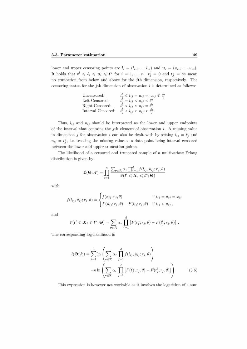
3.3. Parameter estimation 49
lower and upper censoring points are li = (li1, . . . , lid) and ui = (ui1, . . . , uid).It holds that tl 6 li 6 ui 6 tu for i = 1, . . . , n. tl
j = 0 and tuj = ∞ mean
no truncation from below and above for the jth dimension, respectively. Thecensoring status for the jth dimension of observation i is determined as follows:
Uncensored: tlj 6 lij = uij =: xij 6 tu
j
Left Censored: tlj = lij < uij < tu
j
Right Censored: tlj < lij < uij = tu
j
Interval Censored: tlj < lij < uij < tu
j .
Thus, lij and uij should be interpreted as the lower and upper endpointsof the interval that contains the jth element of observation i. A missing valuein dimension j for observation i can also be dealt with by setting lij = tl
j anduij = tu
j , i.e. treating the missing value as a data point being interval censoredbetween the lower and upper truncation points.
The likelihood of a censored and truncated sample of a multivariate Erlangdistribution is given by
L(Θ;X ) =n∏
i=1
∑r∈R αr
∏dj=1 f(lij , uij ; rj , θ)
P(tl 6Xi 6 tu; Θ)
with
f(lij , uij ; rj , θ) =
f(xij ; rj , θ) if lij = uij = xij
F (uij ; rj , θ)− F (lij ; rj , θ) if lij < uij ,
and
P(tl 6Xi 6 tu; Θ) =
∑r∈R
αr
d∏j=1
[F (tu
j ; rj , θ)− F (tlj ; rj , θ)
].
The corresponding log-likelihood is
l(Θ;X ) =n∑
i=1ln
∑r∈R
αr
d∏j=1
f(lij , uij ; rj , θ)
−n ln
∑r∈R
αr
d∏j=1
[F (tu
j ; rj , θ)− F (tlj ; rj , θ)
] . (3.6)
This expression is however not workable as it involves the logarithm of a sum
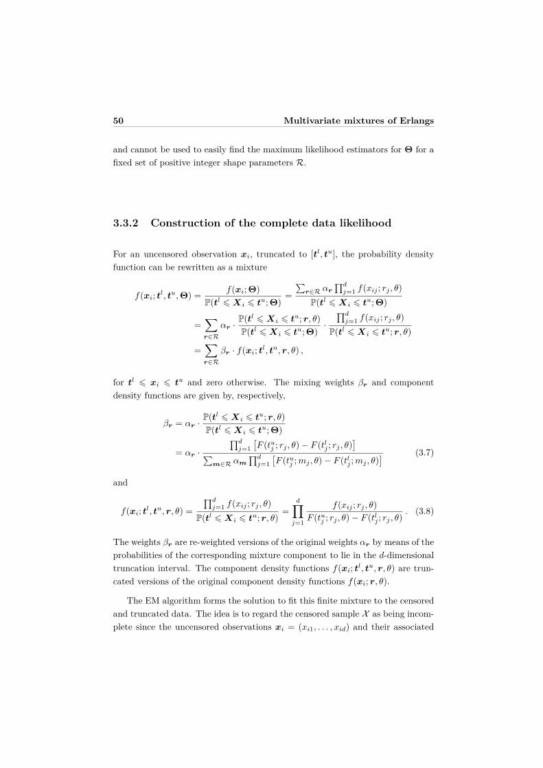
50 Multivariate mixtures of Erlangs
and cannot be used to easily find the maximum likelihood estimators for Θ for afixed set of positive integer shape parameters R.
3.3.2 Construction of the complete data likelihood
For an uncensored observation xi, truncated to [tl, tu], the probability densityfunction can be rewritten as a mixture
f(xi; tl, tu, Θ) = f(xi; Θ)P(tl 6Xi 6 tu; Θ)
=∑
r∈R αr
∏dj=1 f(xij ; rj , θ)
P(tl 6Xi 6 tu; Θ)
=∑r∈R
αr ·P(tl 6Xi 6 tu; r, θ)P(tl 6Xi 6 tu; Θ)
·∏d
j=1 f(xij ; rj , θ)P(tl 6Xi 6 tu; r, θ)
=∑r∈R
βr · f(xi; tl, tu, r, θ) ,
for tl 6 xi 6 tu and zero otherwise. The mixing weights βr and componentdensity functions are given by, respectively,
βr = αr ·P(tl 6Xi 6 tu; r, θ)P(tl 6Xi 6 tu; Θ)
= αr ·∏d
j=1[F (tu
j ; rj , θ)− F (tlj ; rj , θ)
]∑m∈R αm
∏dj=1
[F (tu
j ; mj , θ)− F (tlj ; mj , θ)
] (3.7)
and
f(xi; tl, tu, r, θ) =∏d
j=1 f(xij ; rj , θ)P(tl 6Xi 6 tu; r, θ)
=d∏
j=1
f(xij ; rj , θ)F (tu
j ; rj , θ)− F (tlj ; rj , θ)
. (3.8)
The weights βr are re-weighted versions of the original weights αr by means of theprobabilities of the corresponding mixture component to lie in the d-dimensionaltruncation interval. The component density functions f(xi; tl, tu, r, θ) are trun-cated versions of the original component density functions f(xi; r, θ).
The EM algorithm forms the solution to fit this finite mixture to the censoredand truncated data. The idea is to regard the censored sample X as being incom-plete since the uncensored observations xi = (xi1, . . . , xid) and their associated
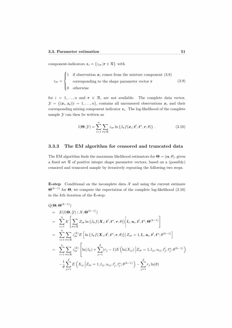
3.3. Parameter estimation 51
component-indicators zi = {zir |r ∈ R} with
zir =
1 if observation xi comes from the mixture component (3.8)
corresponding to the shape parameter vector r
0 otherwise
(3.9)
for i = 1, . . . , n and r ∈ R, are not available. The complete data vector,Y = {(xi, zi)|i = 1, . . . , n}, contains all uncensored observations xi and theircorresponding mixing component indicator zi. The log-likelihood of the completesample Y can then be written as
l(Θ;Y) =n∑
i=1
∑r∈R
zir ln(βrf(xi; tl, tu, r, θ)
). (3.10)
3.3.3 The EM algorithm for censored and truncated data
The EM algorithm finds the maximum likelihood estimators for Θ = (α, θ), givena fixed set R of positive integer shape parameter vectors, based on a (possibly)censored and truncated sample by iteratively repeating the following two steps.
E-step Conditional on the incomplete data X and using the current estimateΘ(k−1) for Θ, we compute the expectation of the complete log-likelihood (3.10)in the kth iteration of the E-step:
Q(Θ; Θ(k−1))
= E(l(Θ;Y) | X ; Θ(k−1))
=n∑
i=1E
[∑r∈R
Zir ln(βrf(Xi; tl, tu, r, θ)
)∣∣∣∣∣ li,ui, tl, tu; Θ(k−1)
]
=n∑
i=1
∑r∈R
z(k)ir E
[ln(βrf(Xi; tl, tu, r, θ)
)∣∣Zir = 1, li,ui, tl, tu; θ(k−1)
]
=n∑
i=1
∑r∈R
z(k)ir
ln(βr) +d∑
j=1(rj − 1)E
(ln(Xij)
∣∣∣Zir = 1, lij , uij , tlj , tu
j ; θ(k−1))
−1θ
d∑j=1
E(
Xij
∣∣∣Zir = 1, lij , uij , tlj , tu
j ; θ(k−1))−
d∑j=1
rj ln(θ)
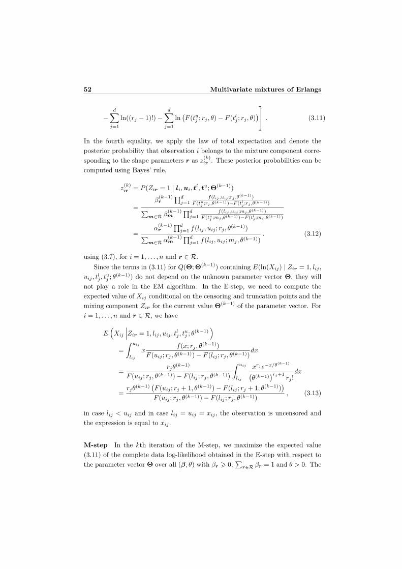
52 Multivariate mixtures of Erlangs
−d∑
j=1ln((rj − 1)!)−
d∑j=1
ln(F (tu
j ; rj , θ)− F (tlj ; rj , θ)
) . (3.11)
In the fourth equality, we apply the law of total expectation and denote theposterior probability that observation i belongs to the mixture component corre-sponding to the shape parameters r as z
(k)ir . These posterior probabilities can be
computed using Bayes’ rule,
z(k)ir = P (Zir = 1 | li,ui, t
l, tu; Θ(k−1))
=β
(k−1)r
∏dj=1
f(lij ,uij ;rj ,θ(k−1))F (tu
j;rj ,θ(k−1))−F (tl
j;rj ,θ(k−1))∑
m∈R β(k−1)m
∏dj=1
f(lij ,uij ;mj ,θ(k−1))F (tu
j;mj ,θ(k−1))−F (tl
j;mj ,θ(k−1))
=α
(k−1)r
∏dj=1 f(lij , uij ; rj , θ(k−1))∑
m∈R α(k−1)m
∏dj=1 f(lij , uij ; mj , θ(k−1))
. (3.12)
using (3.7), for i = 1, . . . , n and r ∈ R.Since the terms in (3.11) for Q(Θ; Θ(k−1)) containing E(ln(Xij) | Zir = 1, lij ,
uij , tlj , tu
j ; θ(k−1)) do not depend on the unknown parameter vector Θ, they willnot play a role in the EM algorithm. In the E-step, we need to compute theexpected value of Xij conditional on the censoring and truncation points and themixing component Zir for the current value Θ(k−1) of the parameter vector. Fori = 1, . . . , n and r ∈ R, we have
E(
Xij
∣∣∣Zir = 1, lij , uij , tlj , tu
j ; θ(k−1))
=∫ uij
lij
xf(x; rj , θ(k−1))
F (uij ; rj , θ(k−1))− F (lij ; rj , θ(k−1))dx
= rjθ(k−1)
F (uij ; rj , θ(k−1))− F (lij ; rj , θ(k−1))
∫ uij
lij
xrj e−x/θ(k−1)(θ(k−1)
)rj+1rj !
dx
=rjθ(k−1) (F (uij ; rj + 1, θ(k−1))− F (lij ; rj + 1, θ(k−1))
)F (uij ; rj , θ(k−1))− F (lij ; rj , θ(k−1))
, (3.13)
in case lij < uij and in case lij = uij = xij , the observation is uncensored andthe expression is equal to xij .
M-step In the kth iteration of the M-step, we maximize the expected value(3.11) of the complete data log-likelihood obtained in the E-step with respect tothe parameter vector Θ over all (β, θ) with βr > 0,
∑r∈R βr = 1 and θ > 0. The
3.3. Parameter estimation 53
maximization with respect to the mixing weights β, requires the maximization of
n∑i=1
∑r∈R
z(k)ir ln(βr) ,
which can be done analogously as in the univariate case, yielding
β(k)r = n−1
n∑i=1
z(k)ir for r ∈ R . (3.14)
The average over the posterior probabilities of belonging to the jth component inthe mixture forms the new estimator for the prior probability βj in the truncatedmixture.
We set the first order partial derivative with respect to θ equal to zero in orderto maximize Q(Θ; Θ(k−1)) over θ (see Appendix 3.7), leading to the following M-step equation:
θ(k) =n−1∑n
i=1∑
r∈R z(k)ir
∑dj=1 E
(Xij
∣∣Zir = 1, lij , uij , tlj , tu
j ; θ(k−1) )− T (k)∑r∈R β
(k)r
∑dj=1 rj
(3.15)
with
T (k) =∑r∈R
β(k)r
d∑j=1
(tlj
)rje−tl
j/θ −(tuj
)rje−tu
j /θ
θrj−1(rj − 1)!(F (tu
j ; rj , θ)− F (tlj ; rj , θ)
)∣∣∣∣∣∣θ=θ(k)
.
Similar to the univariate case (Verbelen et al., 2015), the new estimator θ(k)
in (3.15) for the common scale parameter θ has the interpretation of the expectedtotal mean divided by the weighted total shape parameter in the mixture minusa correction term T (k) due to the truncation. Since T (k) in (3.15) depends onθ(k) and has a complicated form, it is not possible to find an analytical solu-tion. Therefore, we use a Newton-type algorithm, with the previous value of θ,i.e. θ(k−1), as starting value, to solve the equation.
We iterate the E- and M-step until the difference in log-likelihood l(Θ(k);X )−l(Θ(k−1);X ) between two iterations becomes sufficiently small. By inverting ex-pression (3.7), we retrieve the maximum likelihood estimator of the original mixing
54 Multivariate mixtures of Erlangs
weights α(k)r for r ∈ R. We first compute
αr = βr∏dj=1
[F (tu
j ; rj , θ)− F (tlj ; rj , θ)
] for r ∈ R , (3.16)
where βr and θ denote the values in the final EM step, and then normalize theweights such that they sum to 1.
Using the EM algorithm, the log-likelihood (3.6) increases with each itera-tion (McLachlan and Krishnan, 2008). The estimator for Θ = (α, θ) obtainedfrom the EM algorithm has the same limit as the maximum likelihood estimator,whenever the starting value is adequately chosen. Hence, the maximum likelihoodasymptotic theory in terms of consistency, asymptotic normality and asymptoticefficiency applies. Within the EM framework, the asymptotic covariance matrixof the maximum likelihood estimator can be assessed (McLachlan and Krishnan,2008).
These asymptotic results can only be applied with respect to Θ, given a fixedshape set R. However, the number of mixture components and the correspondingvalues of the shape parameter vectors also have to be estimated for which wediscuss a strategy in the next section. The asymptotic results stated here donot take this form of model selection into account. In Section 3.5.3 we applya bootstrap approach to obtain bootstrap confidence intervals for the value ofKendall’s τ and Spearman’s ρ.
3.4 Computational details
An efficient multivariate extension of the univariate EM estimation procedure forErlang mixtures is not straightforward. Indeed, initialization of the parametervalues and model selection are the main difficulties when estimating a multivari-ate Erlang mixture to a data sample and are crucial for its practical use in dataanalysis. We fill this gap and suggest an effective method to initialize the pa-rameters of a multivariate Erlang mixture and a strategy to select the best set ofshape parameter vectors using a model selection criterion.
3.4.1 Initialization and first run of the EM algorithm
Property 1 ensures that any positive continuous distribution can be approximatedby an MME. The formulation of the property also shows how this approximation
3.4. Computational details 55
can be achieved in case the density to be approximated is available. Therefore, itserves as a starting point on how to come up with initial values in case of a sampleof observations. A priori, it is however not clear how to translate the property toa finite sample setting.
Initializing data In a finite sample setting, we do not have the underlyingdensity function at our disposal and initialize the parameters making use of aninitializing data matrix y of dimension n×d which contains xij if the jth elementof observation i is uncensored, lij in the case of right censoring, uij in the caseof left censoring, and (lij + uij)/2 in case of interval censoring. Hence, we usepopular simple imputation techniques (see e.g. Leung et al., 1997) to deal withthe censoring in the initial step. If the jth element of observation i is missing orright censored at 0, we set yij equal to missing.
Shapes For any given initial common scale θ(0), instead of using an infiniteset of positive integer shape parameters in each dimension (cfr. Property 1), werestrict this to a maximum number M of shape parameters in each dimension. Weselect these shape parameters in a sensible way by using M quantiles ranging fromthe minimum to the maximum in each dimension in order to make a data-drivendecision on the locations of the shape parameters. Denoting the p-percent quantileof the initializing data in dimension j by Q(p;yj), and taking into account thatthe expected value of a univariate Erlang distribution with shape r and scale θ
equals rθ, the set of positive integer shapes in dimension j is chosen as
{r1,j , . . . , rMj ,j} ={⌈
Q(p;yj)θ(0)
⌉∣∣∣∣ p = 0,1
M − 1 ,2
M − 1 , . . . , 1}
. (3.17)
where d e denotes upwards rounding, due to the fact that the shapes have tobe positive integers. Consequently, several shapes might coincide which resultsin Mj 6 M shape parameters in dimension j. The initial shape set is then con-structed as the Cartesian product of the d sets of positive integer shape parametersin each dimension:
R = {r1,1, . . . , rM1,1} × · · · × {r1,d, . . . , rMd,d} . (3.18)
Weights The shape parameters in each dimension, multiplied with the com-mon scale parameter θ(0), form a grid that covers the sample range. As an em-pirical version of Property 1, the weights αr, for each shape parameter vector

56 Multivariate mixtures of Erlangs
r = (rm1,1, . . . , rmd,d) in R, with 1 6 mj 6 Mj for all j = 1, . . . , d, are ini-tialized by the relative frequency of data points in the d-dimensional rectangle(rm1−1,1θ(0), rm1,1θ(0)]× · · · × (rmd−1,dθ(0), rmd,dθ(0)] defined by the grid:
α(0)r=(rm1,1,...,rmd,d) = n−1
n∑i=1
d∏j=1
I(
rmj−1,jθ(0) < yij 6 rmj ,jθ(0))
, (3.19)
with r0,j = 0 for notational convenience and the indicator equal to 1/Mj in caseyij is missing. If this hyperrectangle does not contain any data points, the initialweight corresponding to the multivariate Erlang in the mixture with that shapevector will be set equal to zero. Consequently, the weight will remain zero ateach subsequent iteration of the EM algorithm (see formulas (3.12) and (3.14)).Therefore, these shape vectors can immediately be removed from the set R. Atinitialization, the truncation is only taken into account to transform the initialvalues for α into the initial values for β via (3.7).
The maximal number of shape vectors is limited to Md at the initial step.However, due to the fact that Mj 6 M and many shape parameter vectors willreceive an initial weight equal to zero, the actual number of shape vectors at theinitial step will be lower.
Common scale The initial value of the common scale θ is the most influentialfor the performance of the initial multivariate Erlang mixture, as is the case in theunivariate setting (Verbelen et al., 2015). A value which is too large will resultin a multivariate mixture which is too flat (‘underfit’); a value which is too smallwill lead to a mixture which is too peaky (‘overfit’). A priori, it is not evidenthow one can make an insightful decision on θ. Similar to Verbelen et al. (2015),we therefore introduce an additional tuning parameter: an integer spread factors. We propose to initialize the common scale as
θ(0) = minj(maxi(yij))s
. (3.20)
Due to the use of marginal quantiles in (3.17) , the range of the shape parametersvaries according to the sample ranges in each dimension j = 1, . . . , d with amaximum shape parameter equal to
rMj ,j =⌈
maxi(yij)θ(0)
⌉=⌈
maxi(yij)minj(maxi(yij))s
⌉. (3.21)
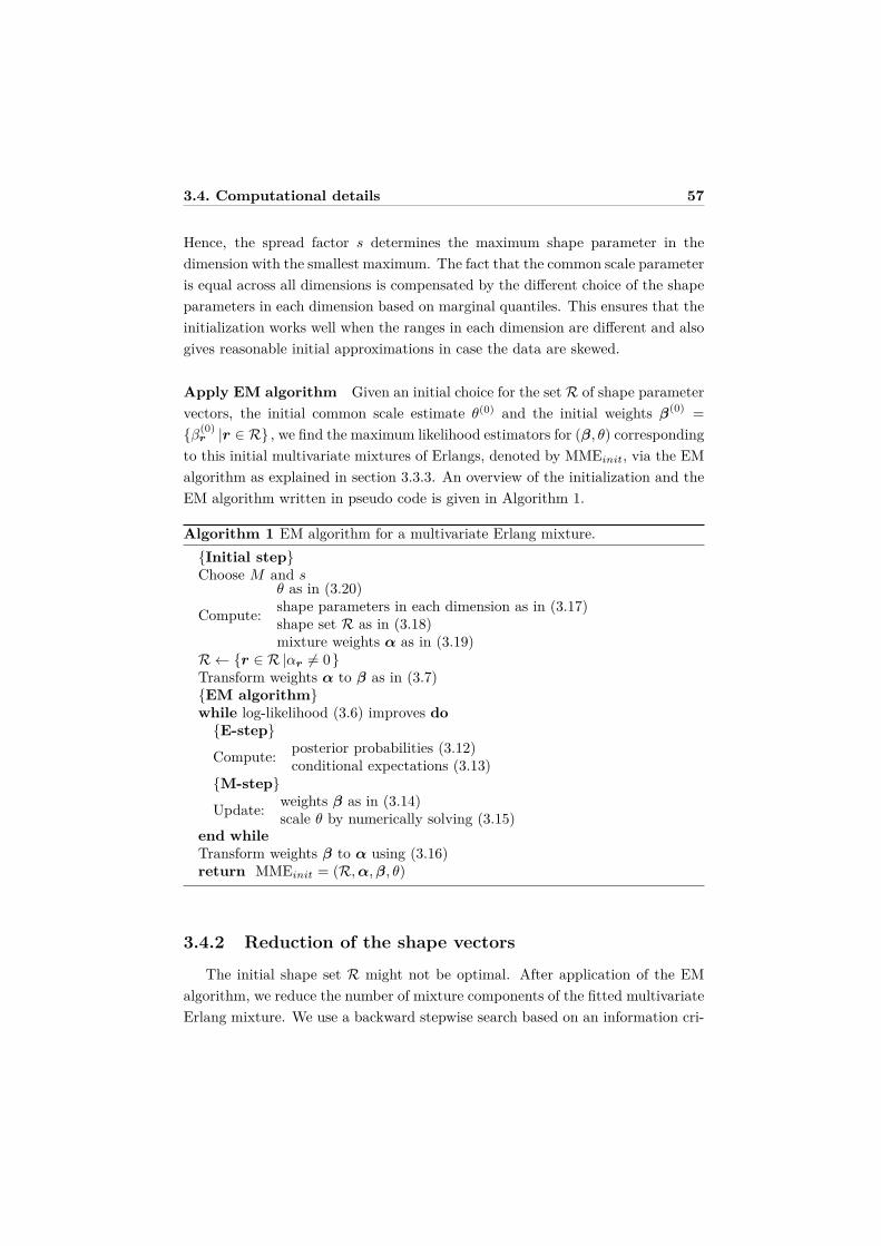
3.4. Computational details 57
Hence, the spread factor s determines the maximum shape parameter in thedimension with the smallest maximum. The fact that the common scale parameteris equal across all dimensions is compensated by the different choice of the shapeparameters in each dimension based on marginal quantiles. This ensures that theinitialization works well when the ranges in each dimension are different and alsogives reasonable initial approximations in case the data are skewed.
Apply EM algorithm Given an initial choice for the set R of shape parametervectors, the initial common scale estimate θ(0) and the initial weights β(0) ={β(0)
r |r ∈ R} , we find the maximum likelihood estimators for (β, θ) correspondingto this initial multivariate mixtures of Erlangs, denoted by MMEinit, via the EMalgorithm as explained in section 3.3.3. An overview of the initialization and theEM algorithm written in pseudo code is given in Algorithm 1.
Algorithm 1 EM algorithm for a multivariate Erlang mixture.{Initial step}Choose M and s
Compute:
θ as in (3.20)shape parameters in each dimension as in (3.17)shape set R as in (3.18)mixture weights α as in (3.19)
R← {r ∈ R |αr 6= 0}Transform weights α to β as in (3.7){EM algorithm}while log-likelihood (3.6) improves do{E-step}
Compute: posterior probabilities (3.12)conditional expectations (3.13)
{M-step}
Update: weights β as in (3.14)scale θ by numerically solving (3.15)
end whileTransform weights β to α using (3.16)return MMEinit = (R,α,β, θ)
3.4.2 Reduction of the shape vectors
The initial shape set R might not be optimal. After application of the EMalgorithm, we reduce the number of mixture components of the fitted multivariateErlang mixture. We use a backward stepwise search based on an information cri-
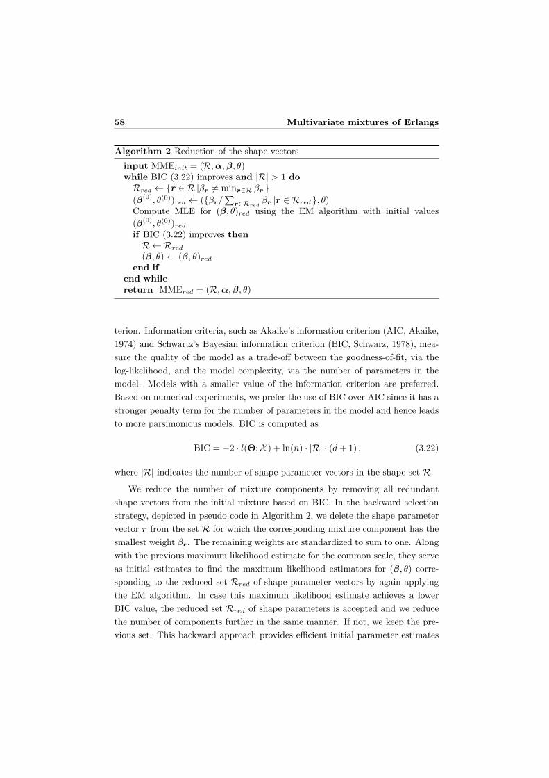
58 Multivariate mixtures of Erlangs
Algorithm 2 Reduction of the shape vectorsinput MMEinit = (R,α,β, θ)while BIC (3.22) improves and |R| > 1 doRred ← {r ∈ R |βr 6= minr∈R βr }(β(0), θ(0))red ← ({βr/
∑r∈Rred
βr |r ∈ Rred }, θ)Compute MLE for (β, θ)red using the EM algorithm with initial values(β(0), θ(0))red
if BIC (3.22) improves thenR← Rred
(β, θ)← (β, θ)red
end ifend whilereturn MMEred = (R,α,β, θ)
terion. Information criteria, such as Akaike’s information criterion (AIC, Akaike,1974) and Schwartz’s Bayesian information criterion (BIC, Schwarz, 1978), mea-sure the quality of the model as a trade-off between the goodness-of-fit, via thelog-likelihood, and the model complexity, via the number of parameters in themodel. Models with a smaller value of the information criterion are preferred.Based on numerical experiments, we prefer the use of BIC over AIC since it has astronger penalty term for the number of parameters in the model and hence leadsto more parsimonious models. BIC is computed as
BIC = −2 · l(Θ;X ) + ln(n) · |R| · (d + 1) , (3.22)
where |R| indicates the number of shape parameter vectors in the shape set R.
We reduce the number of mixture components by removing all redundantshape vectors from the initial mixture based on BIC. In the backward selectionstrategy, depicted in pseudo code in Algorithm 2, we delete the shape parametervector r from the set R for which the corresponding mixture component has thesmallest weight βr. The remaining weights are standardized to sum to one. Alongwith the previous maximum likelihood estimate for the common scale, they serveas initial estimates to find the maximum likelihood estimators for (β, θ) corre-sponding to the reduced set Rred of shape parameter vectors by again applyingthe EM algorithm. In case this maximum likelihood estimate achieves a lowerBIC value, the reduced set Rred of shape parameters is accepted and we reducethe number of components further in the same manner. If not, we keep the pre-vious set. This backward approach provides efficient initial parameter estimates

3.4. Computational details 59
for the reduced set of shape parameter vectors and ensures a fast convergence ofthe EM algorithm.
3.4.3 Adjustment of the shape vectors
Algorithm 3 Adjustment of the shape combinationsinput MMEred = (R,α,β, θ)while log-likelihood (3.6) improves do
for j ∈ {1, . . . , d} dofor r ∈ R do
repeatif (r1, . . . , rj + 1, . . . , rd) /∈ R thenRadj ← {r ∈ R |r 6= r } ∪ {(r1, . . . , rj + 1, . . . , rd)}Compute MLE for (β, θ)adj using the EM algorithm with initialvalues (β, θ)if log-likelihood (3.6) improves thenR← Radj
(β, θ)← (β, θ)adj
end ifend if
until (r1, . . . , rj + 1, . . . , rd) ∈ R or log-likelihood (3.6) no longer im-proves
end forfor r ∈ R do
repeatif (r1, . . . , rj − 1, . . . , rd) /∈ R and rj − 1 > 1 thenRadj ← {r ∈ R |r 6= r } ∪ {(r1, . . . , rj − 1, . . . , rd)}Compute MLE for (β, θ)adj using the EM algorithm with initialvalues (β, θ)if log-likelihood (3.6) improves thenR← Radj
(β, θ)← (β, θ)adj
end ifend if
until (r1, . . . , rj − 1, . . . , rd) ∈ R or rj − 1 = 0 or log-likelihood (3.6)no longer improves
end forend for
end whilereturn MMEadj = (R,α,β, θ)
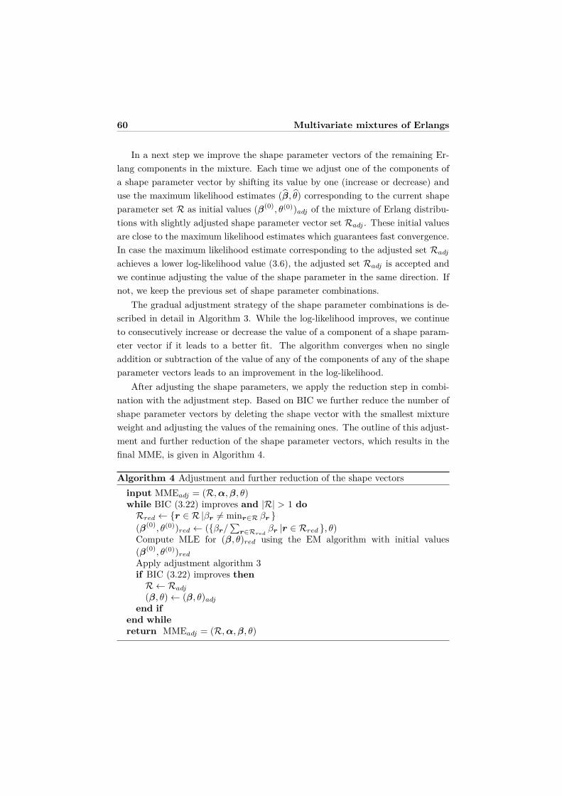
60 Multivariate mixtures of Erlangs
In a next step we improve the shape parameter vectors of the remaining Er-lang components in the mixture. Each time we adjust one of the components ofa shape parameter vector by shifting its value by one (increase or decrease) anduse the maximum likelihood estimates (β, θ) corresponding to the current shapeparameter set R as initial values (β(0), θ(0))adj of the mixture of Erlang distribu-tions with slightly adjusted shape parameter vector set Radj . These initial valuesare close to the maximum likelihood estimates which guarantees fast convergence.In case the maximum likelihood estimate corresponding to the adjusted set Radj
achieves a lower log-likelihood value (3.6), the adjusted set Radj is accepted andwe continue adjusting the value of the shape parameter in the same direction. Ifnot, we keep the previous set of shape parameter combinations.
The gradual adjustment strategy of the shape parameter combinations is de-scribed in detail in Algorithm 3. While the log-likelihood improves, we continueto consecutively increase or decrease the value of a component of a shape param-eter vector if it leads to a better fit. The algorithm converges when no singleaddition or subtraction of the value of any of the components of any of the shapeparameter vectors leads to an improvement in the log-likelihood.
After adjusting the shape parameters, we apply the reduction step in combi-nation with the adjustment step. Based on BIC we further reduce the number ofshape parameter vectors by deleting the shape vector with the smallest mixtureweight and adjusting the values of the remaining ones. The outline of this adjust-ment and further reduction of the shape parameter vectors, which results in thefinal MME, is given in Algorithm 4.
Algorithm 4 Adjustment and further reduction of the shape vectorsinput MMEadj = (R,α,β, θ)while BIC (3.22) improves and |R| > 1 doRred ← {r ∈ R |βr 6= minr∈R βr }(β(0), θ(0))red ← ({βr/
∑r∈Rred
βr |r ∈ Rred }, θ)Compute MLE for (β, θ)red using the EM algorithm with initial values(β(0), θ(0))red
Apply adjustment algorithm 3if BIC (3.22) improves thenR← Radj
(β, θ)← (β, θ)adj
end ifend whilereturn MMEadj = (R,α,β, θ)
3.5. Examples 61
3.5 Examples
We demonstrate the proposed fitting procedure on three data sets, each timehighlighting a different aspect of multivariate mixtures of Erlangs. In a firstsimulated two-dimensional example, we explicitly illustrate the different steps ofthe estimation procedure. Second, we model the waiting time between eruptionsand the duration of the eruptions of the old faithful geyser data set. Based onthe fitted two-dimensional MME, we immediately obtain the distribution of thesum of the waiting time and the duration, representing the total cycle time. Inthe third example, we use multivariate mixtures of Erlangs to model the udderinfection times of dairy cows observed in a mastitis study, and use the fitted MMEto analytically quantify the positive correlation between the udder infection timesusing the explicit expression of the bivariate measures of association Kendall’stau and Spearman’s rho in the MME setting.
The resulting MME after applying the different steps in choosing the shapevectors depends heavily on the starting values. Therefore it is crucial to suffi-ciently explore the effect of changing the value of the tuning parameters M ands and compare the results of several different initial starting points for the shapeset. In addition to the value of BIC, graphs aid the assessment of the fitted model.
3.5.1 Simulated data
As a first example, we generate 1000 uncensored and untruncated observationsfrom a bivariate normal copula with correlation coefficient 0.75 and Erlang dis-tributed margins with shape parameter equal to 2 and 10, respectively, and scaleparameter equal to 3 and 20, resp. A scatterplot of this simulated data set isshown in Figure 3.1a. Due to the parameter choice, the ranges in each dimensionare quite different.
We now apply the different steps of the estimation procedure on this data setand graphically illustrate the interpretations and effects of these steps. First weconsider the initialization strategy for the shape set R, the scale parameter θ andthe mixture weights β, based on the denseness property of MME in Property 1, asexplained in Section 3.4.1. This strategy is controlled by two tuning parameters, amaximum number M of shape parameters in each dimension and a spread factors. In this illustration, we use M = 10 and s = 20. For this choice, the scale θ isinitialized as
θ(0) = minj(maxi(xij))s
= 27.3245220 = 1.366226 .
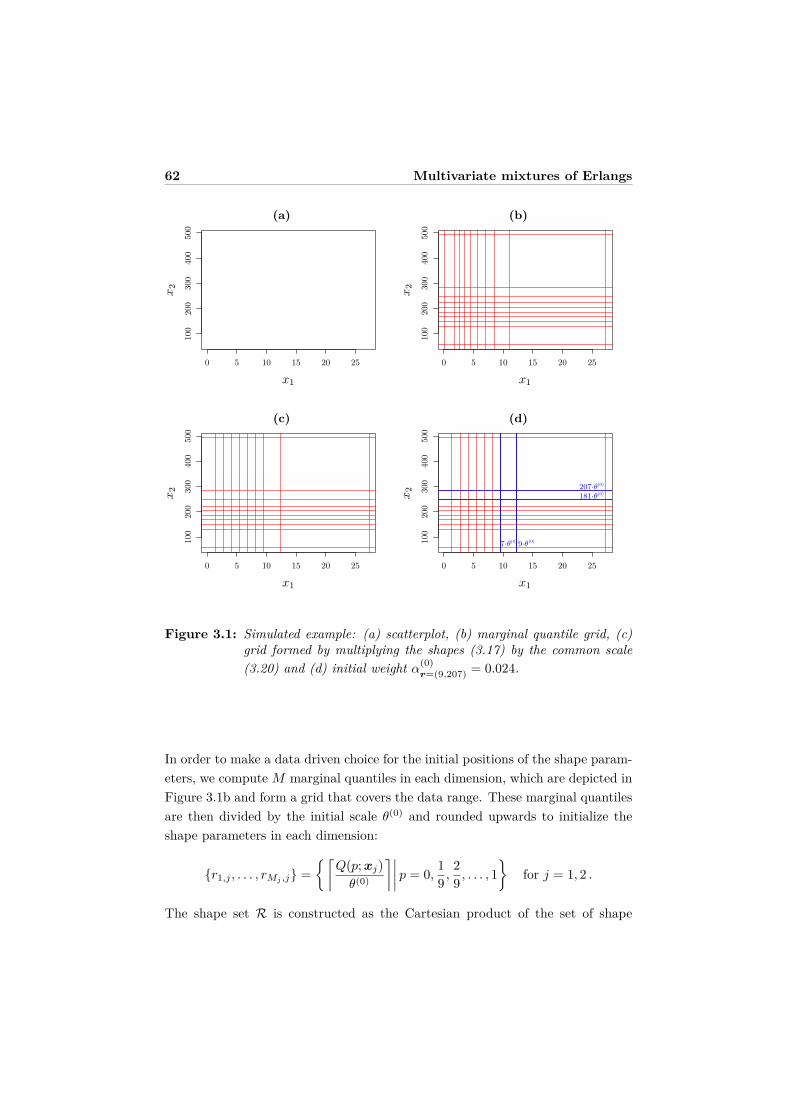
62 Multivariate mixtures of Erlangs
(a)
0 5 10 15 20 25
100
200
300
400
500
x1
x2
(b)
0 5 10 15 20 25
100
200
300
400
500
x1
x2
(c)
0 5 10 15 20 25
100
200
300
400
500
x1
x2
(d)
0 5 10 15 20 25
100
200
300
400
500
x1
x2
9·θ(0)
207·θ(0)
7·θ(0)
181·θ(0)
Figure 3.1: Simulated example: (a) scatterplot, (b) marginal quantile grid, (c)grid formed by multiplying the shapes (3.17) by the common scale(3.20) and (d) initial weight α
(0)r=(9,207) = 0.024.
In order to make a data driven choice for the initial positions of the shape param-eters, we compute M marginal quantiles in each dimension, which are depicted inFigure 3.1b and form a grid that covers the data range. These marginal quantilesare then divided by the initial scale θ(0) and rounded upwards to initialize theshape parameters in each dimension:
{r1,j , . . . , rMj ,j} ={⌈
Q(p;xj)θ(0)
⌉∣∣∣∣ p = 0,19 ,
29 , . . . , 1
}for j = 1, 2 .
The shape set R is constructed as the Cartesian product of the set of shape
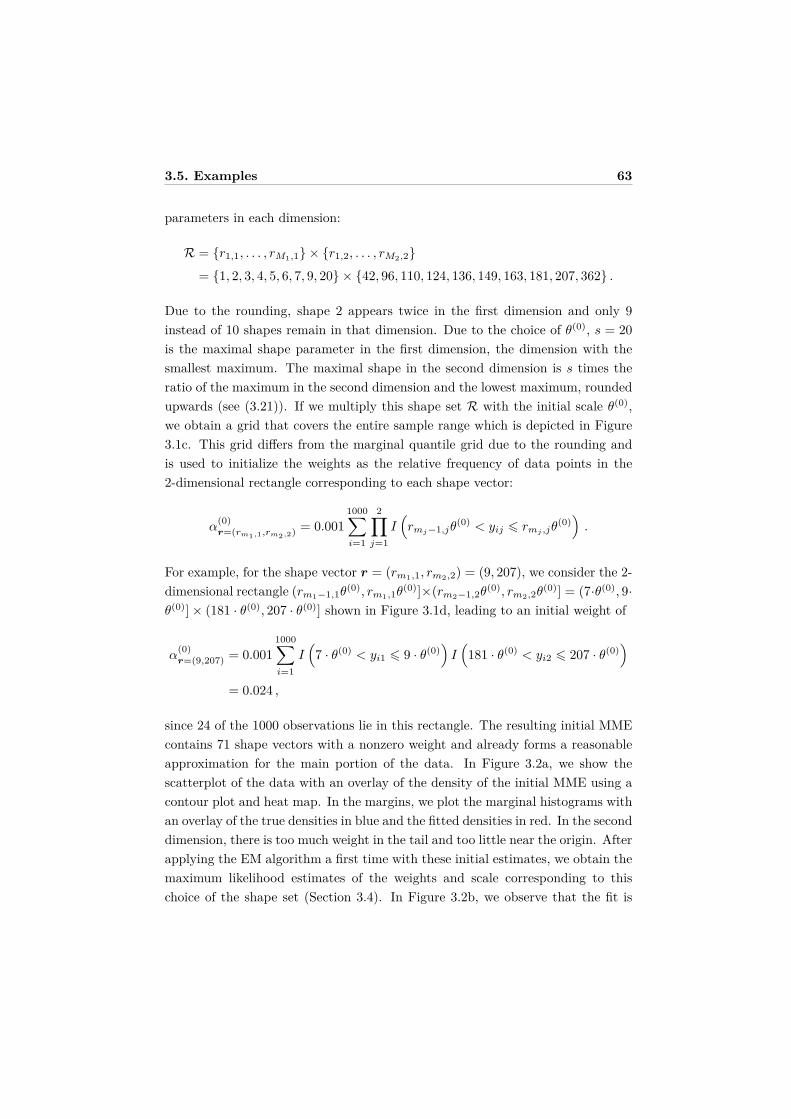
3.5. Examples 63
parameters in each dimension:
R = {r1,1, . . . , rM1,1} × {r1,2, . . . , rM2,2}
= {1, 2, 3, 4, 5, 6, 7, 9, 20} × {42, 96, 110, 124, 136, 149, 163, 181, 207, 362} .
Due to the rounding, shape 2 appears twice in the first dimension and only 9instead of 10 shapes remain in that dimension. Due to the choice of θ(0), s = 20is the maximal shape parameter in the first dimension, the dimension with thesmallest maximum. The maximal shape in the second dimension is s times theratio of the maximum in the second dimension and the lowest maximum, roundedupwards (see (3.21)). If we multiply this shape set R with the initial scale θ(0),we obtain a grid that covers the entire sample range which is depicted in Figure3.1c. This grid differs from the marginal quantile grid due to the rounding andis used to initialize the weights as the relative frequency of data points in the2-dimensional rectangle corresponding to each shape vector:
α(0)r=(rm1,1,rm2,2) = 0.001
1000∑i=1
2∏j=1
I(
rmj−1,jθ(0) < yij 6 rmj ,jθ(0))
.
For example, for the shape vector r = (rm1,1, rm2,2) = (9, 207), we consider the 2-dimensional rectangle (rm1−1,1θ(0), rm1,1θ(0)]×(rm2−1,2θ(0), rm2,2θ(0)] = (7·θ(0), 9·θ(0)]× (181 · θ(0), 207 · θ(0)] shown in Figure 3.1d, leading to an initial weight of
α(0)r=(9,207) = 0.001
1000∑i=1
I(
7 · θ(0) < yi1 6 9 · θ(0))
I(
181 · θ(0) < yi2 6 207 · θ(0))
= 0.024 ,
since 24 of the 1000 observations lie in this rectangle. The resulting initial MMEcontains 71 shape vectors with a nonzero weight and already forms a reasonableapproximation for the main portion of the data. In Figure 3.2a, we show thescatterplot of the data with an overlay of the density of the initial MME using acontour plot and heat map. In the margins, we plot the marginal histograms withan overlay of the true densities in blue and the fitted densities in red. In the seconddimension, there is too much weight in the tail and too little near the origin. Afterapplying the EM algorithm a first time with these initial estimates, we obtain themaximum likelihood estimates of the weights and scale corresponding to thischoice of the shape set (Section 3.4). In Figure 3.2b, we observe that the fit is
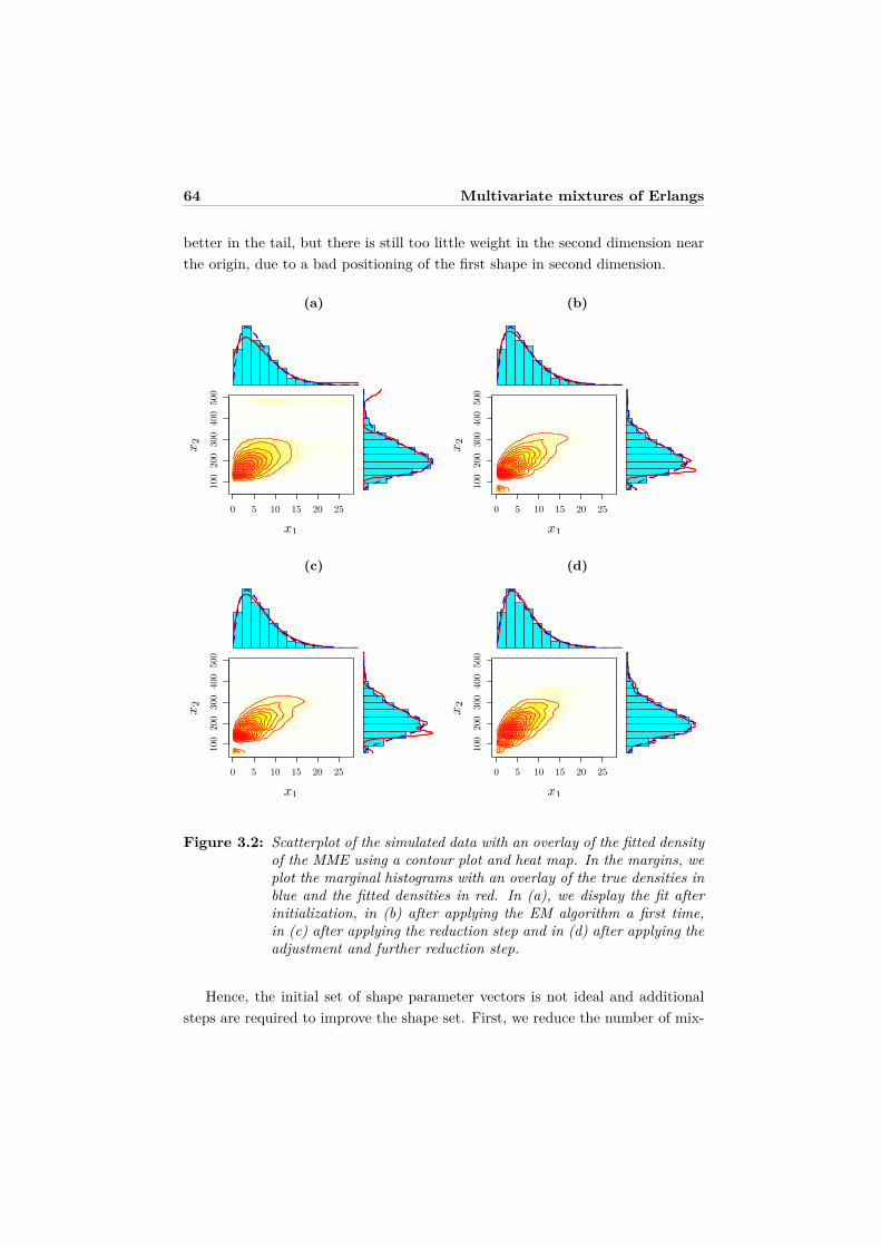
64 Multivariate mixtures of Erlangs
better in the tail, but there is still too little weight in the second dimension nearthe origin, due to a bad positioning of the first shape in second dimension.
(a)
0 5 10 15 20 25
100
200
300
400
500
x1
x2
(b)
0 5 10 15 20 25
100
200
300
400
500
x1
x2
(c)
0 5 10 15 20 25
100
200
300
400
500
x1
x2
(d)
0 5 10 15 20 25
100
200
300
400
500
x1
x2
Figure 3.2: Scatterplot of the simulated data with an overlay of the fitted densityof the MME using a contour plot and heat map. In the margins, weplot the marginal histograms with an overlay of the true densities inblue and the fitted densities in red. In (a), we display the fit afterinitialization, in (b) after applying the EM algorithm a first time,in (c) after applying the reduction step and in (d) after applying theadjustment and further reduction step.
Hence, the initial set of shape parameter vectors is not ideal and additionalsteps are required to improve the shape set. First, we reduce the number of mix-
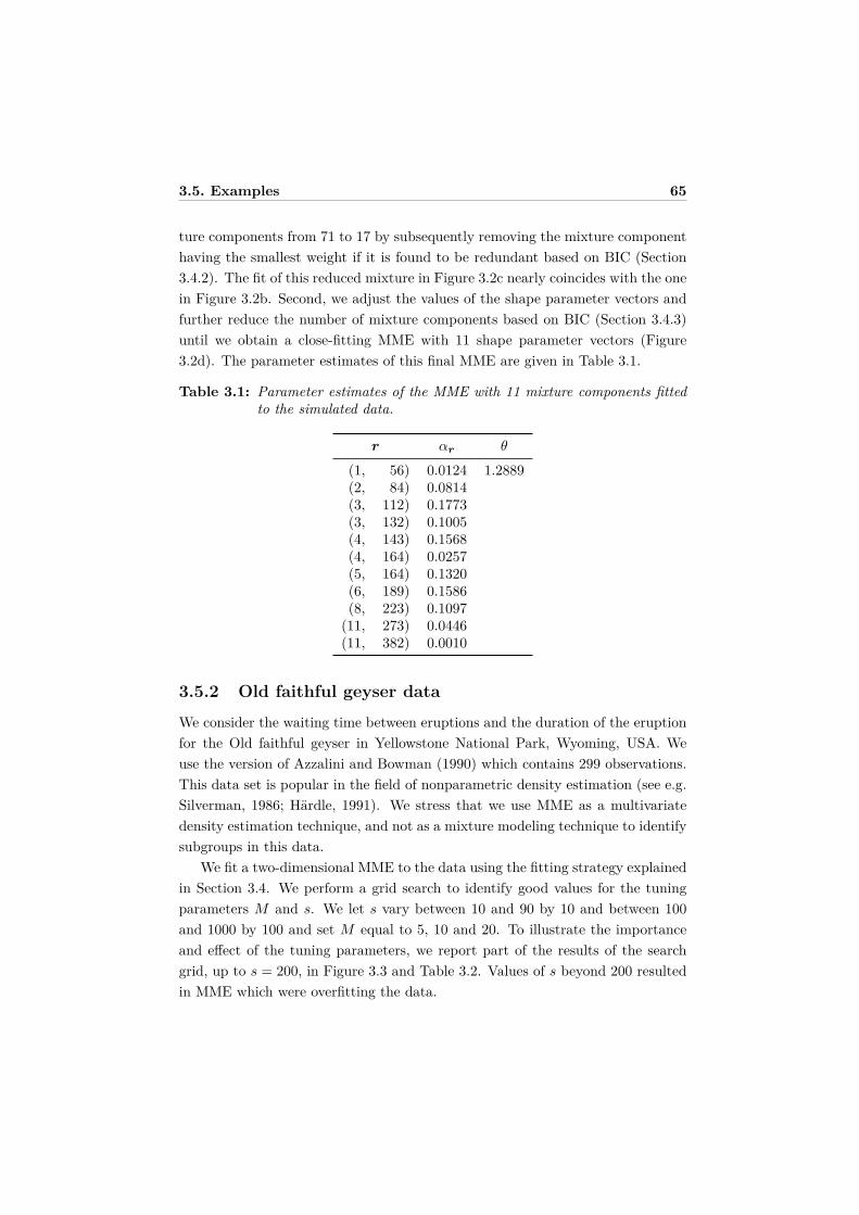
3.5. Examples 65
ture components from 71 to 17 by subsequently removing the mixture componenthaving the smallest weight if it is found to be redundant based on BIC (Section3.4.2). The fit of this reduced mixture in Figure 3.2c nearly coincides with the onein Figure 3.2b. Second, we adjust the values of the shape parameter vectors andfurther reduce the number of mixture components based on BIC (Section 3.4.3)until we obtain a close-fitting MME with 11 shape parameter vectors (Figure3.2d). The parameter estimates of this final MME are given in Table 3.1.
Table 3.1: Parameter estimates of the MME with 11 mixture components fittedto the simulated data.
r αr θ
(1, 56) 0.0124 1.2889(2, 84) 0.0814(3, 112) 0.1773(3, 132) 0.1005(4, 143) 0.1568(4, 164) 0.0257(5, 164) 0.1320(6, 189) 0.1586(8, 223) 0.1097
(11, 273) 0.0446(11, 382) 0.0010
3.5.2 Old faithful geyser data
We consider the waiting time between eruptions and the duration of the eruptionfor the Old faithful geyser in Yellowstone National Park, Wyoming, USA. Weuse the version of Azzalini and Bowman (1990) which contains 299 observations.This data set is popular in the field of nonparametric density estimation (see e.g.Silverman, 1986; Hardle, 1991). We stress that we use MME as a multivariatedensity estimation technique, and not as a mixture modeling technique to identifysubgroups in this data.
We fit a two-dimensional MME to the data using the fitting strategy explainedin Section 3.4. We perform a grid search to identify good values for the tuningparameters M and s. We let s vary between 10 and 90 by 10 and between 100and 1000 by 100 and set M equal to 5, 10 and 20. To illustrate the importanceand effect of the tuning parameters, we report part of the results of the searchgrid, up to s = 200, in Figure 3.3 and Table 3.2. Values of s beyond 200 resultedin MME which were overfitting the data.
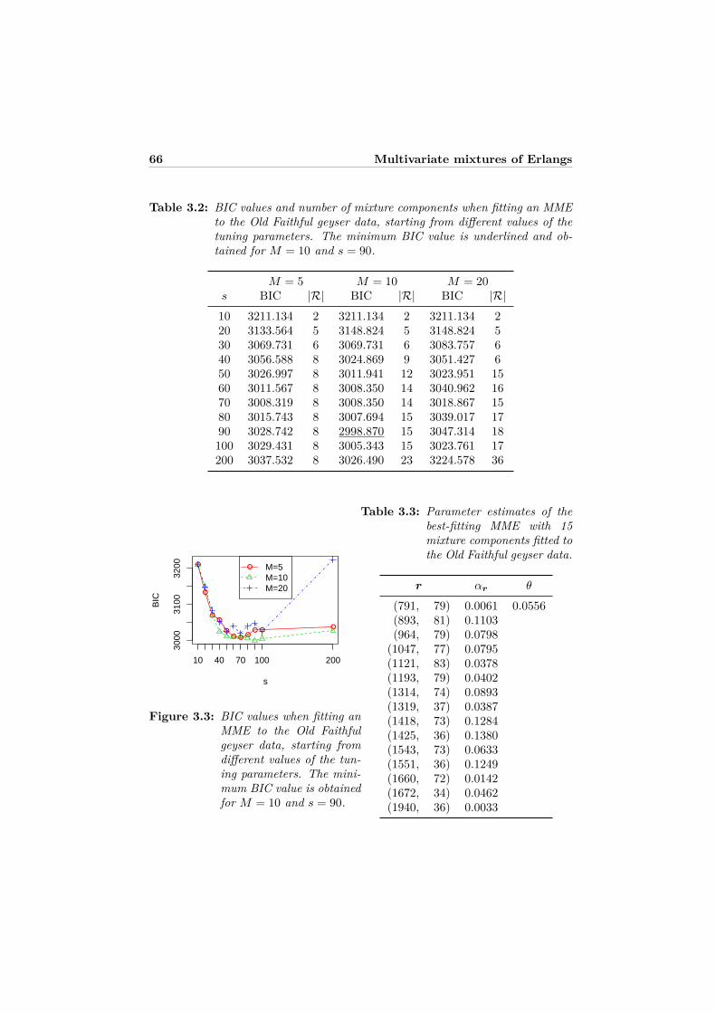
66 Multivariate mixtures of Erlangs
Table 3.2: BIC values and number of mixture components when fitting an MMEto the Old Faithful geyser data, starting from different values of thetuning parameters. The minimum BIC value is underlined and ob-tained for M = 10 and s = 90.
M = 5 M = 10 M = 20s BIC |R| BIC |R| BIC |R|10 3211.134 2 3211.134 2 3211.134 220 3133.564 5 3148.824 5 3148.824 530 3069.731 6 3069.731 6 3083.757 640 3056.588 8 3024.869 9 3051.427 650 3026.997 8 3011.941 12 3023.951 1560 3011.567 8 3008.350 14 3040.962 1670 3008.319 8 3008.350 14 3018.867 1580 3015.743 8 3007.694 15 3039.017 1790 3028.742 8 2998.870 15 3047.314 18100 3029.431 8 3005.343 15 3023.761 17200 3037.532 8 3026.490 23 3224.578 36
3000
3100
3200
s
BIC
10 40 70 100 200
●
●
●●
●● ●
●● ●
●
● M=5M=10M=20
Figure 3.3: BIC values when fitting anMME to the Old Faithfulgeyser data, starting fromdifferent values of the tun-ing parameters. The mini-mum BIC value is obtainedfor M = 10 and s = 90.
Table 3.3: Parameter estimates of thebest-fitting MME with 15mixture components fitted tothe Old Faithful geyser data.
r αr θ
(791, 79) 0.0061 0.0556(893, 81) 0.1103(964, 79) 0.0798
(1047, 77) 0.0795(1121, 83) 0.0378(1193, 79) 0.0402(1314, 74) 0.0893(1319, 37) 0.0387(1418, 73) 0.1284(1425, 36) 0.1380(1543, 73) 0.0633(1551, 36) 0.1249(1660, 72) 0.0142(1672, 34) 0.0462(1940, 36) 0.0033
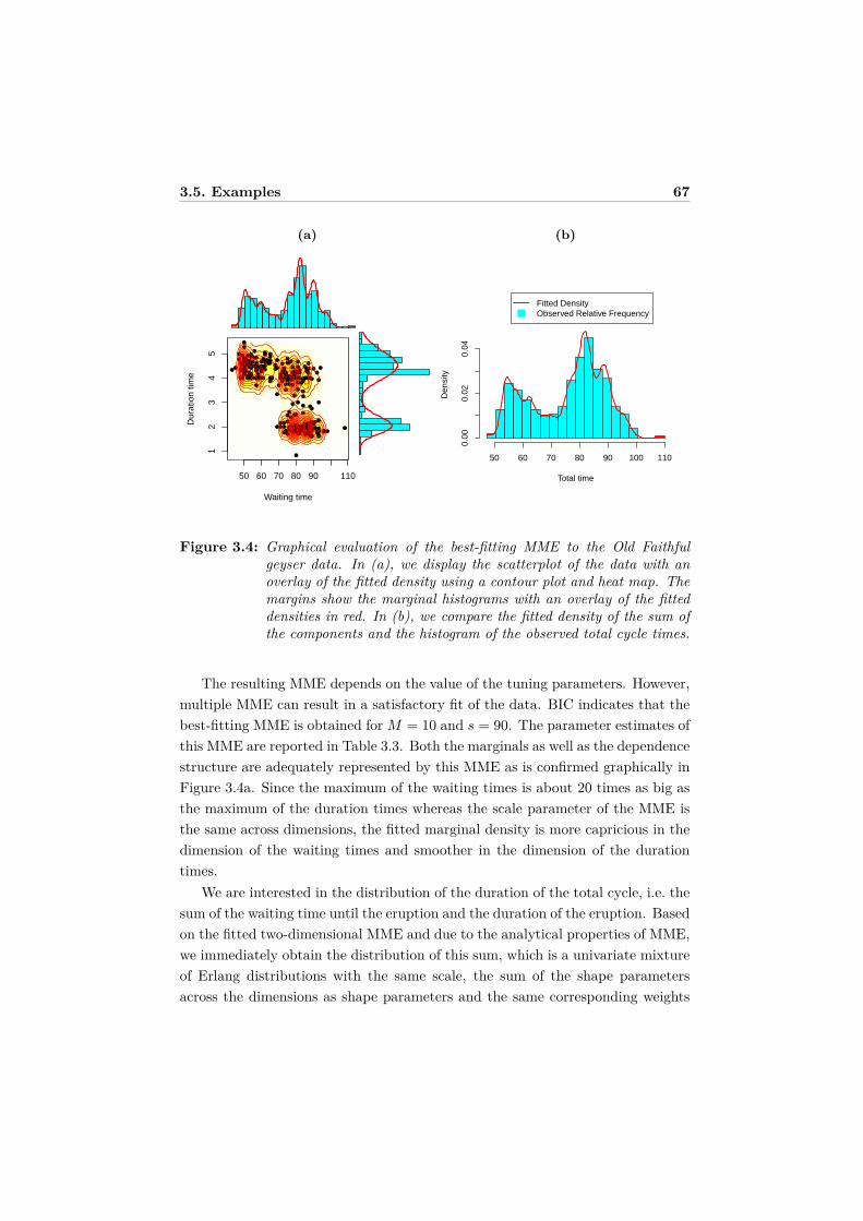
3.5. Examples 67
(a)
●
●
● ●●
●
●●
●
●
●
●
●
●
●
●
●
●
●
●
●
●
●
●
●
●
●
●
●
●
●
●
●
●
●
●
●
●
●
●
●
●
●
●
●
●
●
●
●
●
●
●
●
●
●
●
●
●
●
●
●
●
●
●
●
●
●
●
●
●
●
●
● ●●
●
●
●
●●
●
●
●
●
●
●
●
●
●
●
●
●
●
●
●
●
●
●
●
●
●
●
●
●
●
●
●
●
●
●
●
●
●
●
●
●
●
●
●
●
●
●
●
●
●
● ●
●●
●
●
●
●
●
●
●
●
●
●
●
●
●
●● ●●
●
●
●
●
●
●
●
●
●
●
●
● ●
●
●
● ●
●
●
●
●
●
●
●
●
●
●
●
●
●
●
●
● ●
●
●
●
● ●●●
●
●
●
●
●
●
●
●
●
●
●
●
●
●
●
●
●
●
● ●
●
●
●●
●
●
●
●
●
●
●
●
●
●
●
●●●
●
●●
●
●
●
●
●
●
●
●
●
●
●
●
●
●
●
●
●
●
●
●
●
●
● ●
●
●
●
●
●●
●●
●
●
● ●●
●
●
●
●
●
●
●
●
●
●
●
●●● ●●●●
●
●
●
●
●
●
●
●
●
●
●
●
●
● ●
●
50 60 70 80 90 110
12
34
5
Waiting time
Dur
atio
n tim
e ●
●
● ●●
●
●●
●
●
●
●
●
●
●
●
●
●
●
●
●
●
●
●
●
●
●
●
●
●
●
●
●
●
●
●
●
●
●
●
●
●
●
●
●
●
●
●
●
●
●
●
●
●
●
●
●
●
●
●
●
●
●
●
●
●
●
●
●
●
●
●
● ●●
●
●
●
●●
●
●
●
●
●
●
●
●
●
●
●
●
●
●
●
●
●
●
●
●
●
●
●
●
●
●
●
●
●
●
●
●
●
●
●
●
●
●
●
●
●
●
●
●
●
● ●
●●
●
●
●
●
●
●
●
●
●
●
●
●
●
●● ●●
●
●
●
●
●
●
●
●
●
●
●
● ●
●
●
● ●
●
●
●
●
●
●
●
●
●
●
●
●
●
●
●
● ●
●
●
●
● ●●●
●
●
●
●
●
●
●
●
●
●
●
●
●
●
●
●
●
●
● ●
●
●
●●
●
●
●
●
●
●
●
●
●
●
●
●●●
●
●●
●
●
●
●
●
●
●
●
●
●
●
●
●
●
●
●
●
●
●
●
●
●
● ●
●
●
●
●
●●
●●
●
●
● ●●
●
●
●
●
●
●
●
●
●
●
●
●●● ●●●●
●
●
●
●
●
●
●
●
●
●
●
●
●
● ●
●
(b)
Total time
Den
sity
50 60 70 80 90 100 1100.
000.
020.
04
Fitted DensityObserved Relative Frequency
Figure 3.4: Graphical evaluation of the best-fitting MME to the Old Faithfulgeyser data. In (a), we display the scatterplot of the data with anoverlay of the fitted density using a contour plot and heat map. Themargins show the marginal histograms with an overlay of the fitteddensities in red. In (b), we compare the fitted density of the sum ofthe components and the histogram of the observed total cycle times.
The resulting MME depends on the value of the tuning parameters. However,multiple MME can result in a satisfactory fit of the data. BIC indicates that thebest-fitting MME is obtained for M = 10 and s = 90. The parameter estimates ofthis MME are reported in Table 3.3. Both the marginals as well as the dependencestructure are adequately represented by this MME as is confirmed graphically inFigure 3.4a. Since the maximum of the waiting times is about 20 times as big asthe maximum of the duration times whereas the scale parameter of the MME isthe same across dimensions, the fitted marginal density is more capricious in thedimension of the waiting times and smoother in the dimension of the durationtimes.
We are interested in the distribution of the duration of the total cycle, i.e. thesum of the waiting time until the eruption and the duration of the eruption. Basedon the fitted two-dimensional MME and due to the analytical properties of MME,we immediately obtain the distribution of this sum, which is a univariate mixtureof Erlang distributions with the same scale, the sum of the shape parametersacross the dimensions as shape parameters and the same corresponding weights

68 Multivariate mixtures of Erlangs
in (Lee and Lin, 2012, Theorem 5.1). Hence, the parameters of this univariatemixture of Erlang distributions are readily available from Table 3.3. Comparingthe histogram of the observed total times to the fitted density in Figure 3.4breveals a close approximation.
3.5.3 Mastitis study
Mastitis is economically one of the most important diseases in the dairy sectorsince it leads to reduced milk yield and milk quality. In this example, we considerinfectious disease data from a mastitis study by Laevens et al. (1997). This dataset has also been used in Goethals et al. (2009) and Ampe et al. (2012).
We focus on the infection times of individual cow udder quarters with a bac-terium. As each udder quarter is separated from the three other quarters, onequarter might be infected while the other quarters remain infection-free. However,the dependence must be modeled since the data are hierarchical, with individualobservations at the udder quarter level being correlated within the cow. Addition-ally, the infection times are not known exactly due to a period follow-up, which isoften the case in observational studies since a daily checkup would not be feasible.Roughly each month, the udder quarters are sampled and the infection status isassessed, from the time of parturition, at which the cow was included in the cohortand assumed to be infection-free, until the end of the lactation period. This gen-erates interval-censored data since for udder quarters that experience an event itis only known that the udder quarter got infected between the last visit at whichit was infection-free and the first visit at which it was infected. Observationscan also be right censored if no infection occurred before the end of the lactationperiod, which is roughly 300-350 days but different for every cow, before the endof the study or if the cow is lost to follow-up during the study, for example dueto culling.
The data we consider contains information on 100 dairy cows on the time toinfection of the four udder quarters by different types of bacteria. This data setis used in Goethals et al. (2009), who model the data using an extended sharedgamma frailty model that is able to handle the interval censoring and clusteringsimultaneously. We treat the infection times at the udder quarter level of thecow as four-dimensional interval and right censored data of which we estimatethe underlying density using MME. The udder quarters are denoted as RL (rearleft), FL (front left), RR (rear right) and FR (front right).
In search for the best values of the tuning parameters in the MME estimation
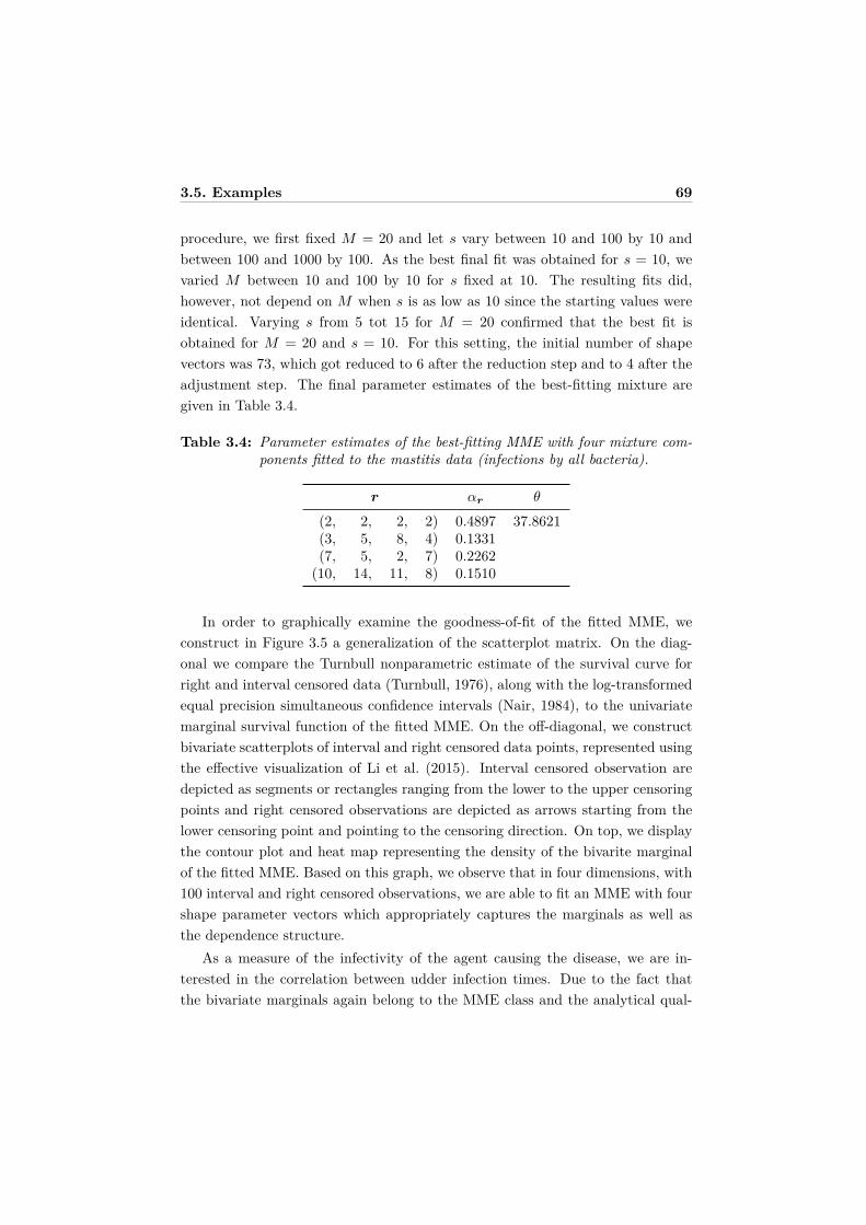
3.5. Examples 69
procedure, we first fixed M = 20 and let s vary between 10 and 100 by 10 andbetween 100 and 1000 by 100. As the best final fit was obtained for s = 10, wevaried M between 10 and 100 by 10 for s fixed at 10. The resulting fits did,however, not depend on M when s is as low as 10 since the starting values wereidentical. Varying s from 5 tot 15 for M = 20 confirmed that the best fit isobtained for M = 20 and s = 10. For this setting, the initial number of shapevectors was 73, which got reduced to 6 after the reduction step and to 4 after theadjustment step. The final parameter estimates of the best-fitting mixture aregiven in Table 3.4.
Table 3.4: Parameter estimates of the best-fitting MME with four mixture com-ponents fitted to the mastitis data (infections by all bacteria).
r αr θ
(2, 2, 2, 2) 0.4897 37.8621(3, 5, 8, 4) 0.1331(7, 5, 2, 7) 0.2262
(10, 14, 11, 8) 0.1510
In order to graphically examine the goodness-of-fit of the fitted MME, weconstruct in Figure 3.5 a generalization of the scatterplot matrix. On the diag-onal we compare the Turnbull nonparametric estimate of the survival curve forright and interval censored data (Turnbull, 1976), along with the log-transformedequal precision simultaneous confidence intervals (Nair, 1984), to the univariatemarginal survival function of the fitted MME. On the off-diagonal, we constructbivariate scatterplots of interval and right censored data points, represented usingthe effective visualization of Li et al. (2015). Interval censored observation aredepicted as segments or rectangles ranging from the lower to the upper censoringpoints and right censored observations are depicted as arrows starting from thelower censoring point and pointing to the censoring direction. On top, we displaythe contour plot and heat map representing the density of the bivarite marginalof the fitted MME. Based on this graph, we observe that in four dimensions, with100 interval and right censored observations, we are able to fit an MME with fourshape parameter vectors which appropriately captures the marginals as well asthe dependence structure.
As a measure of the infectivity of the agent causing the disease, we are in-terested in the correlation between udder infection times. Due to the fact thatthe bivariate marginals again belong to the MME class and the analytical qual-
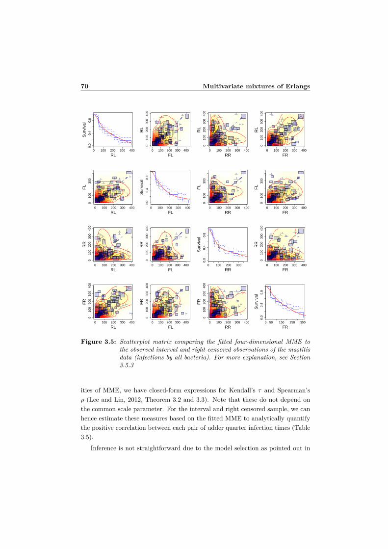
70 Multivariate mixtures of Erlangs
0 100 200 300 400
0.0
0.4
0.8
RL
Sur
viva
l
0 100 200 300 400
010
030
0
RL
FL
FL missing
RL m
issing
0 100 200 300 400
010
020
030
040
0
RL
RR
RR missing
RL m
issing
0 100 200 300 400
010
020
030
040
0
RL
FR
FR missing
RL m
issing
0 100 200 300 4000
100
200
300
400
FL
RL
RL missing
FL m
issing
0 100 200 300 400
0.0
0.4
0.8
FL
Sur
viva
l
0 100 200 300 400
010
020
030
040
0
FL
RR
RR missing
FL m
issing
0 100 200 300 400
010
020
030
040
0
FL
FR
FR missing
FL m
issing
0 100 200 300 400
010
020
030
040
0
RR
RL
RL missing
RR
missing
0 100 200 300 4000
100
300
RR
FL
FL missing
RR
missing
0 100 200 300
0.0
0.4
0.8
RR
Sur
viva
l
0 100 200 300 400
010
020
030
040
0
RR
FR
FR missing
RR
missing
0 100 200 300 400
010
020
030
040
0
FR
RL
RL missing
FR
missing
0 100 200 300 400
010
030
0
FR
FL
FL missing
FR
missing
0 100 200 300 4000
100
200
300
400
FR
RR
RR missing
FR
missing
0 50 150 250 350
0.0
0.4
0.8
FR
Sur
viva
l
Figure 3.5: Scatterplot matrix comparing the fitted four-dimensional MME tothe observed interval and right censored observations of the mastitisdata (infections by all bacteria). For more explanation, see Section3.5.3
ities of MME, we have closed-form expressions for Kendall’s τ and Spearman’sρ (Lee and Lin, 2012, Theorem 3.2 and 3.3). Note that these do not depend onthe common scale parameter. For the interval and right censored sample, we canhence estimate these measures based on the fitted MME to analytically quantifythe positive correlation between each pair of udder quarter infection times (Table3.5).
Inference is not straightforward due to the model selection as pointed out in

3.6. Discussion 71
Section 3.3.3. In order to quantify the uncertainty and construct an approximateconfidence interval for the bivariate measures of association, we resort to a boot-strapping procedure (Efron and Tibshirani, 1994). By sampling with replacementfrom the original four-dimensional data set of size 100, we generate 1000 boot-strap samples of the same size 100. For each of these bootstrap samples, we fit anMME where we set the tuning parameter M equal to 20 and let s vary between5 and 25. We choose this fixed grid for each bootstrap sample since the optimaltuning parameters for the full sample were M = 20 and s = 10 and the startingvalues are not that sensitive with respect to M for low values of s. We therebyobtain 1000 estimates for each measure of association. The 5% and 95% quantilesof these estimates are used to construct a 90% bootstrap percentile confidenceinterval for each Kendall’s τ and Spearman’s ρ in Table 3.5.
Table 3.5: Estimates and 90% bootstrap confidence intervals for the bivariatemeasures of association Kendall’s τ and Spearman’s ρ based on thefitted MME for the mastitis data (infections by all bacteria).
RL FL RR
FL τ 0.4187(0.3329, 0.5515)
ρ 0.6019(0.4727, 0.7439)
RR τ 0.2018 0.3307(0.1693, 0.3989) (0.2585, 0.4784)
ρ 0.3004 0.4852(0.2423, 0.5616) (0.3806, 0.6664)
FR τ 0.4326 0.4105 0.2119(0.3598, 0.5538) (0.2701, 0.4883) (0.1543, 0.3968)
ρ 0.6354 0.5994 0.3122(0.5066, 0.7608) (0.3875, 0.6794) (0.2206, 0.5577)
3.6 Discussion
MME form a highly flexible class of distributions which are at the same timemathematically tractable. From Property 1, we know that any positive contin-uous multivariate distribution can be approximated up to any accuracy by aninfinite multivariate mixture of Erlang distributions. Our contribution presentsa computationally efficient initialization and adjustment strategy for the shapeparameter vectors, translating this theoretical aspect in a strong point in practice
72 Multivariate mixtures of Erlangs
as well. In the examples, we demonstrate how the fitting procedure is able to esti-mate an MME that adequately represents both the marginals and the dependencestructure. By extending the EM algorithm, we are now also able to deal with left,interval or right censored and truncated data. MME therefore form a valuablemultivariate density estimation technique to analyze realistic data, even in incom-plete data settings, and to model the dependence directly in a low dimensionalsetting.
Their tractability allows to derive explicit expression of properties of interest.Willmot and Woo (2015) have paved the way for applying MME in insuranceloss modeling, survival analysis and ruin theory. When modeling insurance lossesor dependent risks from different portfolios or lines of business using MME, theaggregate and excess losses have again a univariate and multivariate mixture ofErlangs distribution. Stop-loss moments, several types of premiums, risk capitalallocation based on the Tail-Value-at-Risk (TVaR) or covariance rule for regu-latory risk capital requirements (see e.g. Dhaene et al., 2012) have analyticalexpressions. When modeling bivariate lifetimes and pricing joint-life and last-survivor insurance (see e.g. Frees et al., 1996) using MME, the distribution of theminimum and maximum is again a univariate mixture of Erlangs. Such kind ofdata are always left truncated and right censored. The extension of the fittingprocedure for MME presented in this chapter, allows to take the right censoringinto account. Left truncation can only be properly handled when the left trun-cation points are fixed for each observation. This is however not the case whenpricing joint-life and last-survivor insurance since the ages at which policyholdersenter a contract vary.
The reduction and adjustment steps of the shape parameters in the fittingprocedure iteratively make use of the EM algorithm and can be time consuming.Further adjustment is needed to estimate parameters in high dimensional settings.As also acknowledged in the univariate case (Verbelen et al., 2015), the modelingof heavy-tailed distributions using MME is challenging since MME are not ableto extrapolate the heaviness in the tail.
3.7 Appendix: Partial derivative of Q
In order to maximize Q(Θ; Θ(k−1)) with respect to θ, we set the first order partialderivative at θ(k) equal to zero. In the second equation, expression (3.2) of thecumulative distribution of an Erlang, while (3.14) is used to obtain the thirdequation.

3.7. Appendix: Partial derivative of Q 73
∂Q(Θ; Θ(k−1))∂θ
∣∣∣∣∣θ=θ(k)
=n∑
i=1
∑r∈R
z(k)ir
(∑dj=1 E
(Xij
∣∣Zir = 1, lij , uij , tlj , tu
j ; θ(k−1) )θ2
−∑d
j=1 rj
θ−
d∑j=1
∂∂θ
[F (tu
j ; rj , θ)− F (tlj ; rj , θ)
]F (tu
j ; rj , θ)− F (tlj ; rj , θ)
∣∣∣∣∣∣θ=θ(k)
= 1θ2
n∑i=1
∑r∈R
z(k)ir
d∑j=1
E(
Xij
∣∣∣Zir = 1, lij , uij , tlj , tu
j ; θ(k−1))
−n
θ
∑r∈R
(∑ni=1 z
(k)ir
n
)d∑
j=1rj
−n∑
i=1
∑r∈R
z(k)ir
d∑j=1
∂∂θ
(γ(rj , tu
j /θ)− γ(rj , tlj/θ)
)(rj − 1)!
(F (tu
j ; rj , θ)− F (tlj ; rj , θ)
)∣∣∣∣∣∣θ=θ(k)
= 1θ2
n∑i=1
∑r∈R
z(k)ir
d∑j=1
E(
Xij
∣∣∣Zir = 1, lij , uij , tlj , tu
j ; θ(k−1))
−n
θ
∑r∈R
β(k)r
d∑j=1
rj
− n
θ2
∑r∈R
β(k)r
d∑j=1
(tlj
)rje−tl
j/θ −(tuj
)rje−tu
j /θ
θrj−1(rj − 1)!(F (tu
j ; rj , θ)− F (tlj ; rj , θ)
)∣∣∣∣∣∣θ=θ(k)
= 0 ,
where we used expression (3.2) of the cumulative distribution of an Erlang in thesecond equality and (3.14) in the third.


Chapter 4
Unraveling the predictive power
of telematics data in car insurance
pricing
Abstract
A data set from a Belgian telematics product aimed at young drivers is usedto identify how car insurance premiums can be designed based on the telem-atics data collected by a black box installed in the vehicle. In traditionalpricing models for car insurance, the premium depends on self-reported rat-ing variables (e.g. age, postal code) which capture characteristics of thepolicy(holder) and the insured vehicle and are often only indirectly relatedto the accident risk. Using telematics technology enables tailor-made carinsurance pricing based on the driving behavior of the policyholder. We de-velop a statistical modeling approach using generalized additive models andcompositional predictors to quantify and interpret the effect of telematicsvariables on the expected claim frequency. We find that such variables in-crease the predictive power and render the use of gender as a discriminatingrating variable redundant.
This chapter is based on Verbelen, R., Antonio, K., and Claeskens, G. (2016).Unraveling the predictive power of telematics data in car insurance pricing. FEBResearch Report KBI 1624.
75
76 Telematics insurance
4.1 Introduction
For a unique Belgian portfolio of young drivers in the period between 2010 and2014, telematics data on how many kilometers are driven, during which time slotsand on which type of roads were collected using black box devices installed inthe insureds’ cars. The aim in this chapter is to incorporate this information instatistical rating models, where we focus on predicting the number of claims, inorder to adequately set premium levels based on individual policyholder’s drivinghabits.
Determining a fair and correct price for an insurance product (also calledratemaking, pricing or tarification) is crucial for both insureds and insurancecompanies. Pricing through risk classification or segmentation is the mechanisminsurance companies use to compete and to reduce the price of insurance contracts.Insurance Europe, the European insurance and reinsurance federation, reports1 atotal motor premium income amounting to e124 billion in 2014. Car insuranceis the most widely purchased non-life insurance product in Europe, accountingfor 27.3% of non-life premiums. To avoid lapses in this competitive market manyrating factors are used to classify risks and differentiate prices. Besides the fiercecompetition, high acquisition and retention costs, low customer engagement, nobrand loyalty and a high cost of retention have put a huge pressure on the carinsurance industry. Car insurance is traditionally priced based on self-reportedinformation from the insured, most importantly: age, license age, postal code,engine power, use of the vehicle, and claims history. However, these observable riskfactors are only proxy variables, not reflecting present patterns of driving habitsand the driving style, and consequently tariff cells are still quite heterogeneous.
Telematics technology – the integrated use of telecommunication and infor-matics – may fundamentally change the car insurance industry. The use of thistechnology in insured vehicles enables to transmit and receive information thatallows an insurance company to better quantify the accident risk of drivers andadjust the premiums accordingly through usage-based insurance (UBI). By moni-toring their customers’ motoring habits, underwriters can increasingly distinguishbetween drivers who are safe on the road from those who merely seem safe on pa-per.2 Young drivers and drivers in other high risk groups, who are typically facinghefty insurance premiums, can be judged based on how they really drive. Regu-lation also plays a role as the use of indirect indicators of risk is being questioned
1 http://www.insuranceeurope.eu/european-motor-insurance-markets-addendum2 How’s my driving? (2013, February 23) The Economist. http: // econ. st/ Yd5x3C
4.1. Introduction 77
by the European Court of Justice. In 2012, a European Union (EU) ruling cameinto force, banning price differentiation based on gender.3 Through telematics,women may be able to confirm that they really are safer drivers.
The use of telematics risk factors potentially enables an improved method fordetermining the cost of insurance. Due to a more refined customer segmentationand greater monitoring of the driving behavior, UBI addresses the problems ofadverse selection and moral hazard that arise from the information asymmetrybetween the insurer and the policyholders (Filipova-Neumann and Welzel, 2010).Closer aligning insurance policies to the actual risks increases actuarial fairnessand reduces cross-subsidization compared to grouping the drivers into too generalactuarial classes (Desyllas and Sako, 2013). In addition, some positive exter-nalities are to be expected (Parry, 2005; Litman, 2015; Tselentis et al., 2016).Telematics insurance gives a high incentive to change the current driving patternand stimulates more responsible driving. Users’ feedback on driving behavior andgamification of UBI can further enhance the customer experience by making itmore interactive, gratifying and even exciting (Toledo et al., 2008). Less andsafer driving is encouraged, leading to improved road safety and reduced vehicletravel with less congestion, pollution, fuel consumption, road cost, and crashes(Greenberg, 2009).
Usage-based insurance includes Pay-as-you-drive (PAYD) and pay-how-you-drive (PHYD) schemes (Tselentis et al., 2016). PAYD focuses on the drivinghabits, e.g. the driven distance, the time of day, how long the insured has beendriving, and the location. PHYD goes even further by also considering the drivingstyle, e.g. the speed, harsh or smooth braking, aggressive acceleration or decelera-tion, cornering and parking skills. Furthermore, the telematics data collected canbe enriched using other sources of data, for example road maps with correspondingspeed limitations to infer road types and speeding violations.
Telematics insurance started as a niche market when the technology first sur-faced more than 10 years ago. The high implementation costs and its complexitylimited its success. Advances in technology and telecommunication have how-ever reduced the cost substantially. Early adopters of UBI were seen primarily inthe United States (US), Italy and the United Kingdom (UK) due to the higherpremiums, particularly for young drivers, the highly competitive markets, and ahigher incidence of fraudulent claims and vehicle theft. Monti’s decree of 20124,
3 http://europa.eu/rapid/press-release_IP-11-1581_en.htm4 Law Decree of 24 January 2012, n.1 “Urgent provisions for competition, infrastructure de-
velopment and competitiveness” (the so-called “Cresci Italia”), converted by law 24 March2012, n.27.
78 Telematics insurance
encouraging Italian insurers to provide a telematics option, has made Italy themost active country in Europe in telematics insurance, with the overall pene-tration level around 15% in June 2016.5 Ptolemus further reports that at thatmoment insurance companies have launched 292 telematics programs or activetrials worldwide (see Husnjak et al., 2015, for some examples of UBI solutionsimplemented worldwide). The number of UBI policies is over 7.9 million in theUS, over 5 million in Italy and over 860 000 in the UK.6 Moreover, on 28 April2015 the European Parliament voted in favor of eCall regulation which forces allnew cars in the EU from April 2018 onwards to be equipped with a telematics de-vice that will automatically dial 112 in the event of an accident, providing preciselocation and impact data.7 However, legislation also gives rise to legal concernsand challenges in the telematics insurance market. In particular, insurers haveto comply with the aspects of data protection and privacy in the evolving legalenvironment.
This potentially high dimensional telematics data, collected on the fly, forcespricing actuaries to change their current practice, both from a business as wellas a statistical point of view. New statistical models have to be developed to ad-equately set premiums based on an individual policyholder’s driving habits andstyle and the current literature on insurance rating does not adequately addressthis question. In this chapter, we take a first step in this direction. We use a Bel-gian telematics insurance data set with in total over 297 million kilometers driven.Based on how many kilometers the insured drives, on which kind of roads andduring which moments in the day, we quantify the impact of individual drivinghabits on expected claim frequencies. Combined with a similar predictive modelfor claim severities, which is outside of the scope in this chapter, this allows fortailor-made car insurance pricing. We first discuss how a car insurance policy istraditionally priced and relate this to the literature investigating the impact ofvehicle usage on the accident risk in Section 4.2. The data set is described in Sec-tion 4.3, along with the necessary preliminary data processing steps to combinethe telematics information with the policy and claims information. By construct-ing predictive models for the claim frequency, we compare the performance ofdifferent sets of predictor variables (e.g. traditional vs. purely telematics) andunravel the relevance and impact of adding telematics insights. In particular, we
5 http://www.ptolemus.com/ubi-study/telematics-insurance-infographic/6 Ptolemus Consulting Group (2016). Usage-based insurance (global study), free abstract.7 Regulation (EU) 2015/758 of the European Parliament and of the Council of 29 April 2015
concerning type-approval requirements for the deployment of the eCall in-vehicle system basedon the 112 service and amending Directive 2007/46/EC.
4.2. Statistical background and related modeling literature 79
contrast the use of time and distance as exposure-to-risk measures. The statis-tical methodology, including in particular the challenges when incorporating thedivisions of the driven distance by road type and time slots as predictors in themodel, is presented in Section 4.4. In Section 4.5, we present the results and,finally, in Section 4.6, we conclude.
4.2 Statistical background and related modelingliterature
Insurance pricing is the calculation of a fair premium, given the policy(holder)characteristics, as well as information on claims reported in the past (if available).The pure premium represents the expected cost of the claims a policyholder willdeclare during the insured period. Pricing relies on regression techniques andrequires a data set with policy(holder) information and corresponding claim fre-quencies and severities, where severity is the ultimate total impact of a claim.
A priori pricing refers to the statistical problem of pricing without incorpo-rating the claim history of the policyholder, thus neither frequency nor severityof past claims is taken into account. The construction of an a priori tariff tra-ditionally relies on a frequency-severity modeling framework in which the claimfrequency and severity components are typically modeled separately using re-gression techniques (Frees, 2014). A policyholder’s pure premium is obtainedby multiplying the expected claim frequency and expected claim severity, giventhe observable risk factors. The current state-of-the-art (see Denuit et al., 2007;de Jong and Heller, 2008, for an overview) uses generalized linear models (GLMs;McCullagh and Nelder, 1989), with typically a Poisson GLM for the claim countsand a gamma GLM for the claim severities. Modeling the claim severities is dif-ficult, since only those observations corresponding to policyholders who filed aclaim can be used to estimate the claim severity model and due to the complexityof the phenomenon (Denuit and Charpentier, 2005). On the one hand, there is along delay to assess the cost of bodily injury and other severe claims and on theother hand the cost of an accident is, for most part, beyond the control of thedriver. In practice, covariates are much less informative to predict claim amountsthan to predict frequency (Boucher and Charpentier, 2014).
A posteriori pricing refers to experience rating systems which penalize or re-ward policyholders based on (usually) the number of claims reported in the past.The idea is that, over time, insurers try to refine their a priori risk classification
80 Telematics insurance
and restore fairness using no-claim discounts and claim penalties. A bonus-malussystem is a typical example (Lemaire, 1995). A bonus-malus scale consists a finitenumber of levels, each with its own relativity that is applied to the base premium.Transitional rules determine how a policy moves up or down based on the numberof claims at fault. As such, on the basis of the insured’s individual claim experi-ence, the amount of the premium is adjusted each year with penalties in the formof premium surcharges (corresponding to higher bonus-malus levels) for one ormore accidents in the current year and rewards in the form of premium discounts(corresponding to lower bonus-malus levels) for claim-free policyholders. From astatistical point of view a posteriori rating requires the analysis of multilevel data(Gelman and Hill, 2007).
In car insurance, the duration of the policy period during which coverage isprovided, is referred to as the exposure-to-risk, the basic rating unit underlying theinsurance premium. The expected number of claims is in practice modeled directlyproportional to the exposure. The logic behind this is to make the premiumsproportional to the length of coverage. As such, a premium related to an insuredperiod of 6 months will be half of the one-year premium, for a given risk profile.From a theoretical point of view, this can also be motivated by the probabilisticframework of Poisson processes (Denuit et al., 2007). It is however suggested(see e.g. Butler, 1993) that every kilometer traveled by a vehicle transfers risk toits insurer and hence the number of driven kilometers (car-kilometer) should beadopted as the exposure unit instead of the policy duration (car-year). Statisticalstudies show how claim frequencies significantly increase with kilometers (Bordoffand Noel, 2008; Ferreira and Minikel, 2010; Litman, 2011; Boucher et al., 2013;Lemaire et al., 2016). Most of these studies show a relationship between claimfrequencies and the number of driven kilometers which is less than proportional.They suggest that possibly high-kilometer drivers are more experienced, havenewer and safer vehicles, or drive more on low-risk motorways rather than high-risk urban areas.
Data collected using telematics technology offers more insight in the drivinghabits. Instead of relying only on the self-reported annual number of drivenkilometers, pay-as-you-drive insurance can also account for the type of road andthe time of the day when an insured has been driving. A next step is to alsotake data on driving style into account, leading to a pay-how-you-drive insurance(Weiss and Smollik, 2012). Statistical analysis of these types of data has been thesubject of limited academic scrutiny.
Ayuso et al. (2014, 2016a) study the traveled time and distance to the first
4.3. Telematics insurance data 81
accident using Weibull regression models involving both policy and telematicspredictors. Paefgen et al. (2014) investigate the relationship between the accidentrisk and driving habits using logistic regression models. Their case-control studydesign does not allow for inference on the probability of accident involvement.The difference in time exposure between the vehicles with accident involvement(6 months prior to the accident) and the control group (24 months) is howeveronly used to obtain a per-month distance exposure, but is further neglected in thestudy. Traditional risk factors were not accounted for, since that information wasnot available, and the compositional nature of the constructed telematics predic-tor variables was ignored. In contrast, combining the new telematics variableswith traditional policy(holder) information through a careful model and variableselection process as well as recognizing the compositional structure in the analysisare main focus points in our research, see Section 4.3.2.
4.3 Telematics insurance data
We consider data from a Belgian portfolio of drivers with motor third party li-ability (MTPL) insurance. MTPL insurance is the legally compulsory minimuminsurance covering damage to third parties’ health and property caused by anaccident for which the driver of the vehicle is responsible. The special type ofMTPL product we are considering, is specifically aiming for young drivers whoare traditionally facing high insurance premiums. Insureds were offered a sub-stantial discount on their premium if they agree to install a telematics black boxdevice in their car. The telematics box collects statistics on the driving habits:how often one drives, how many kilometers, where and when. Information onthe driving style (such as speeding, braking, accelerating, cornering or parking) isnot registered. The telematics data have so far no effect on the (future) premiumlevels of the insureds and do not induce any restrictions on how much or wherethey can drive.
4.3.1 Data processing
The unstructured telematics data, collected by the telematics box installed in thevehicle, are first transmitted to the data provider who structures and aggregatesthese data each day and then reports them to the insurance company as a CSVfile (Figure 4.1a). Only the structured, aggregated telematics information is avail-able to us. Each daily file contains information on the daily driven distance (in
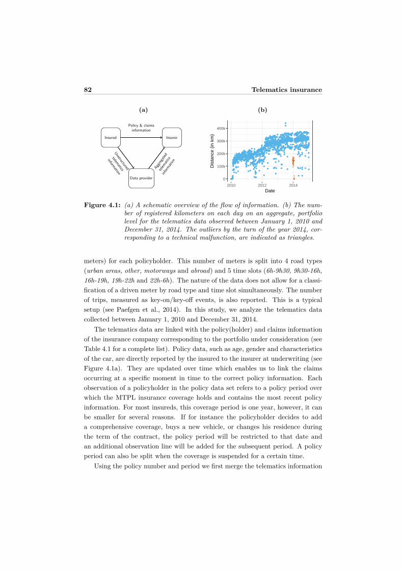
82 Telematics insurance
(a)
Insured Insurer
Data provider
Policy & claimsinformation
Unstructured
telematics
information
Aggre
gated
telem
atics
inform
ation
(b)
●
●
●
●
●
●●●●●●
●
●●●●●
●
●●●●●●●
●
●
●
●●●●
●
●●●●●●●●●
●●
●●●
●●
●●
●●●●
●●
●
●
●●●●
●●
●
●
●
●●
●●
●●●●●
●●
●
●●●●
●●
●
●●●●
●
●
●●
●
●●
●●
●●●●●
●●
●●●●
●
●
●
●
●●●●
●
●
●
●●●●
●●
●
●●
●
●
●●
●
●●●●
●●
●●●●●
●●
●
●●
●●
●●
●
●
●
●●
●
●
●●●●●
●
●
●
●●●●
●●
●●●●●
●
●
●●●●●
●●
●●●●●
●●
●●●
●●
●●
●
●●●●
●●
●
●●●●
●●
●●●●●
●●
●
●●●●
●●
●●●●●
●●
●
●●●●
●●
●●●●●
●●
●
●●●●
●●
●
●●●●
●
●
●●●●●
●
●
●●●●●
●●
●●●●●
●
●
●
●●●●
●
●
●
●●●●
●
●
●
●
●●●
●●
●
●●
●
●
●
●
●
●●●●
●
●
●
●●●●
●
●
●
●●●●
●
●
●
●●●●
●
●
●
●●●●
●
●
●
●
●
●
●
●
●●
●●●
●●
●●
●●●●
●●
●
●●●●
●
●
●
●●●●
●
●
●
●●●●
●
●
●
●●●●
●
●
●
●
●
●●
●●
●
●●●●
●
●
●
●●●●
●
●
●
●●●●
●
●
●●●●●
●
●
●
●●●●
●
●
●
●●
●
●
●
●
●
●●●●
●
●
●
●●
●●●
●
●●●●●
●●
●
●●●●
●
●
●●
●●●
●
●
●
●●●●
●
●
●●●●●●
●
●
●●●●●
●
●
●●●●
●
●
●
●
●●
●●
●
●
●●●●
●
●
●
●
●●●●
●
●
●●●●●
●
●
●
●
●
●
●
●
●
●●●●●
●
●●●●●●
●
●●
●
●
●
●
●
●
●
●
●●●
●
●
●
●
●
●
●
●
●
●●●●●
●
●
●
●●●●
●
●●●●●●
●
●
●●●●●
●
●
●●●●●
●
●
●●●●●
●
●
●●●●●
●
●●●●●●
●
●
●●●●●
●
●
●●●●●
●
●
●●●
●
●
●
●
●●●●●
●
●●
●
●●
●
●
●
●●
●
●
●
●
●
●●●●●
●
●
●●●●●
●
●
●●●●●
●
●
●●●●●
●
●
●●●●●
●
●
●●●●
●
●
●
●
●●●
●
●
●●
●●
●●
●
●
●●●●●
●
●
●●●●●
●
●
●●●●●
●
●
●●●●
●
●
●
●●●
●
●
●
●
●●●●●
●
●
●●●●
●
●
●
●●●●
●
●
●
●●●●●
●
●
●●●●
●
●
●
●●●●
●
●
●
●●●●
●
●
●●●●
●
●
●
●
●●●
●
●
●
●●●●
●
●
●
●●●●
●
●●
●
●
●
●●
●
●
●
●
●
●●
●
●
●
●●
●
●
●●
●
●●
●●
●
●
●
●
●●●
●
●
●
●●●●
●
●
●
●●●●
●
●
●
●●●●
●
●●
●●
●
●
●●
●●●●●
●●
●
●●●●
●
●
●
●●●●
●
●
●
●●●●
●
●
●
●●●●
●
●
●
●●●●
●
●
●
●
●
●
●
●●
●●●●●
●
●
●
●●●●
●
●
●
●●●●
●
●
●
●●●●
●
●
●
●●●●
●
●
●
●
●
●
●
●
●
●
●●
●●
●
●
●
●●●●
●
●
●
●●
●
●
●
●
●
●●●●
●
●
●
●●
●
●
●
●
●
●●●●
●
●
●
●
●
●●
●
●
●
●
●
●
●
●
●
●
●●●●
●
●
●
●●●●●●
●
●●●●
●
●
●
●●●●
●
●
●●
●
●●
●
●
●
●
●
●
●
●
●
●
●
●
●●
●
●
●
●
●
●●
●
●
●
●
●●
●
●●●
●●●●
●
●
●
●●●●
●
●
●
●●●●
●
●
●
●●●●
●
●
●
●●●●
●
●
●
●●●●
●
●
●
●
●
●
●
●
●
●
●●●●
●
●
●
●
●
●●
●
●
●●
●●●
●
●
●
●●●●
●
●
●●●
●●
●
●
●
●●
●●
●
●
●
●
●
●
●
●
●
●
●●
●
●
●
●
●
●●●●
●
●
●
●
●●●
●
●
●
●●●●
●
●
●
●
●●●
●
●
●
●●●●
●
●
●
●●●●
●
●
●
●●
●●
●
●
●
●●●●
●●
●●●●●
●●
●
●
●●●
●●
●
●
●●●
●●
●
●●●●
●
●
●●●●
●
●●
●
●
●
●
●
●
●
●
●●●●
●
●
●
●●●●
●
●
●
●●●●
●
●
●
●●●●
●
●
●
●
●●●
●
●
●
●●●●
●
●
●
●●●●
●
●
●
●●●●
●
●
●
●●●●
●
●
●
●●●●
●
●
●
●●●
●
●
●
●
●●●●
●
●
●●
●●●
●
●
●
●●●●
●
●
●
●●●●
●
●
●
●●●●
●
●
●
●●●●
●
●
●
●
●●
●●
●
●
●
●●●●
●
●
●
●●●●
●
●
●
●●●●
●
●
●
●●●●
●
●
●
●●●●
●●
●
●●●●
●
●
●
●●●●
●
●
●
●●●●
●
●
●
●●●●
●
●
●
●●●●
●●
●
●●●
●
●
●
●
●
●●●
●
●
●
●●
●
●
●
●
●
●●●
●
●
●
●
●●
●●
●
●
●
●●●●
●
●
●
●●●
●
●
●
●
●●●●
●
●
●
●
●
●
●
●
●
●
●●●●
●
●
●
●●●
●
●
●
●
●●
●●
●
●
●
●
●●
●
●
●
●
●●●●
●●
●●
●
●
●
●
●
●
●●●●
●
●
●
●●●●
●
●
●
●●●
●
●
●
●
●●●●
●
●
●
●●●●
●
●
●
●●●●
●
●
●
●●●●
●
●
●
●●●●
●
●
●
●●●●
●
●
●
●●●●
●
●
●
●
●
●
●
●
●
●
●●●●
●
●
●
●●●●
●
●
●
●●
●
●
●
●
●
●●●●
●
●
●
●
●
●●
●
●
●
●●●●
●
●
●
●●●●
●
●
●
●●●●
●
●
●
●●●
●
●
●
●
●
●●●
●
●
●
●●
●
●
●
●
●
●
●●
0
100k
200k
300k
400k
2010 2012 2014
Date
Dis
tanc
e (in
km
)Figure 4.1: (a) A schematic overview of the flow of information. (b) The num-
ber of registered kilometers on each day on an aggregate, portfoliolevel for the telematics data observed between January 1, 2010 andDecember 31, 2014. The outliers by the turn of the year 2014, cor-responding to a technical malfunction, are indicated as triangles.
meters) for each policyholder. This number of meters is split into 4 road types(urban areas, other, motorways and abroad) and 5 time slots (6h-9h30, 9h30-16h,16h-19h, 19h-22h and 22h-6h). The nature of the data does not allow for a classi-fication of a driven meter by road type and time slot simultaneously. The numberof trips, measured as key-on/key-off events, is also reported. This is a typicalsetup (see Paefgen et al., 2014). In this study, we analyze the telematics datacollected between January 1, 2010 and December 31, 2014.
The telematics data are linked with the policy(holder) and claims informationof the insurance company corresponding to the portfolio under consideration (seeTable 4.1 for a complete list). Policy data, such as age, gender and characteristicsof the car, are directly reported by the insured to the insurer at underwriting (seeFigure 4.1a). They are updated over time which enables us to link the claimsoccurring at a specific moment in time to the correct policy information. Eachobservation of a policyholder in the policy data set refers to a policy period overwhich the MTPL insurance coverage holds and contains the most recent policyinformation. For most insureds, this coverage period is one year, however, it canbe smaller for several reasons. If for instance the policyholder decides to adda comprehensive coverage, buys a new vehicle, or changes his residence duringthe term of the contract, the policy period will be restricted to that date andan additional observation line will be added for the subsequent period. A policyperiod can also be split when the coverage is suspended for a certain time.
Using the policy number and period we first merge the telematics information
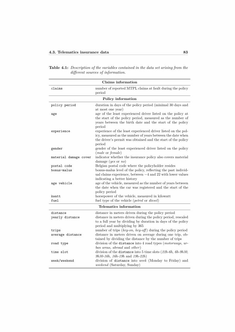
4.3. Telematics insurance data 83
Table 4.1: Description of the variables contained in the data set arising from thedifferent sources of information.
Claims informationclaims number of reported MTPL claims at fault during the policy
periodPolicy information
policy period duration in days of the policy period (minimal 30 days andat most one year)
age age of the least experienced driver listed on the policy atthe start of the policy period, measured as the number ofyears between the birth date and the start of the policyperiod
experience experience of the least experienced driver listed on the pol-icy, measured as the number of years between the date whenthe driver’s permit was obtained and the start of the policyperiod
gender gender of the least experienced driver listed on the policy(male or female)
material damage cover indicator whether the insurance policy also covers materialdamage (yes or no)
postal code Belgian postal code where the policyholder residesbonus-malus bonus-malus level of the policy, reflecting the past individ-
ual claims experience, between −4 and 22 with lower valuesindicating a better history
age vehicle age of the vehicle, measured as the number of years betweenthe date when the car was registered and the start of thepolicy period
kwatt horsepower of the vehicle, measured in kilowattfuel fuel type of the vehicle (petrol or diesel)
Telematics informationdistance distance in meters driven during the policy periodyearly distance distance in meters driven during the policy period, rescaled
to a full year by dividing by duration in days of the policyperiod and multiplying by 365
trips number of trips (key-on, key-off ) during the policy periodaverage distance distance in meters driven on average during one trip, ob-
tained by dividing the distance by the number of tripsroad type division of the distance into 4 road types (motorways, ur-
ban areas, abroad and other)time slot division of the distance into 5 time slots (22h-6h, 6h-9h30,
9h30-16h, 16h-19h and 19h-22h)week/weekend division of distance into week (Monday to Friday) and
weekend (Saturday, Sunday)

84 Telematics insurance
on daily level with the policy data set. Next, we adjust the start and end dateof the policy periods based on the first and last day at which telematics data areobserved for each policy period of each insured. This ensures that the adjustedpolicy periods reflect time periods over which both the insurance coverage holdsand telematics data are collected. Based on Figure 4.1b, where we plot the evolu-tion of the driven distance on each day by all drivers of the portfolio, we suspectthat technical deficiencies of the data provider can cause an underreporting ofthe number of meters driven on an aggregate level. The outliers indicated astriangles by the turn of the year 2014 could be linked to a serious technical failurepreventing telematics information from being reported for a significant part of ourportfolio. We dealt with this by removing this period of roughly one month fromthe policy periods of all insureds. In the remainder of the observation periodbetween January 1, 2010 and December 31, 2014, clear causes of underreport-ing could not be identified and hence we did not take any other corrective action.However, this illustrates that data reliability forms a challenge for this new telem-atics technology. We further removed those observations with a policy durationof less than 30 days in order to avoid senseless observations of only a couple ofdays and retained only the complete observations with no missing policyholderinformation.
Next, we aggregate the telematics information by policyholder and period.This means that we sum the driven distance, their divisions into 4 road types and5 time slots, and the number of trips made. Finally, we use the claims informationto link the number of MTPL claims at fault that occurred between the start andend date of the adjusted policy periods for each policy record.
Over the time period of this study, we end up with a data set of 33 259 observa-tions. Table 4.1 gives an overview of the available variables coming from the threedata sources (claims, policy, and telematics). These observations correspond to10 406 unique policyholders, who are followed over time, have jointly driven over297 million kilometers during a combined insured policy period of 17 681 yearsand reported 1481 MTPL claims at fault. Hence, on average, there were 0.0838claims per insured year or 0.0499 claims per 10 000 driven kilometers. For over95% of the observations no claim occurred during the corresponding policy period,whereas for 52 observations two claims occurred and for a single observation eventhree during the same policy period.
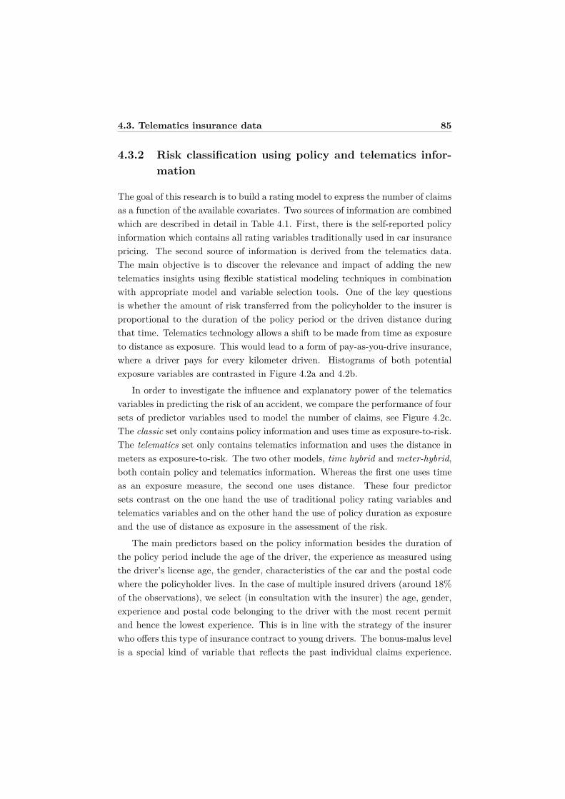
4.3. Telematics insurance data 85
4.3.2 Risk classification using policy and telematics infor-mation
The goal of this research is to build a rating model to express the number of claimsas a function of the available covariates. Two sources of information are combinedwhich are described in detail in Table 4.1. First, there is the self-reported policyinformation which contains all rating variables traditionally used in car insurancepricing. The second source of information is derived from the telematics data.The main objective is to discover the relevance and impact of adding the newtelematics insights using flexible statistical modeling techniques in combinationwith appropriate model and variable selection tools. One of the key questionsis whether the amount of risk transferred from the policyholder to the insurer isproportional to the duration of the policy period or the driven distance duringthat time. Telematics technology allows a shift to be made from time as exposureto distance as exposure. This would lead to a form of pay-as-you-drive insurance,where a driver pays for every kilometer driven. Histograms of both potentialexposure variables are contrasted in Figure 4.2a and 4.2b.
In order to investigate the influence and explanatory power of the telematicsvariables in predicting the risk of an accident, we compare the performance of foursets of predictor variables used to model the number of claims, see Figure 4.2c.The classic set only contains policy information and uses time as exposure-to-risk.The telematics set only contains telematics information and uses the distance inmeters as exposure-to-risk. The two other models, time hybrid and meter-hybrid,both contain policy and telematics information. Whereas the first one uses timeas an exposure measure, the second one uses distance. These four predictorsets contrast on the one hand the use of traditional policy rating variables andtelematics variables and on the other hand the use of policy duration as exposureand the use of distance as exposure in the assessment of the risk.
The main predictors based on the policy information besides the duration ofthe policy period include the age of the driver, the experience as measured usingthe driver’s license age, the gender, characteristics of the car and the postal codewhere the policyholder lives. In the case of multiple insured drivers (around 18%of the observations), we select (in consultation with the insurer) the age, gender,experience and postal code belonging to the driver with the most recent permitand hence the lowest experience. This is in line with the strategy of the insurerwho offers this type of insurance contract to young drivers. The bonus-malus levelis a special kind of variable that reflects the past individual claims experience.
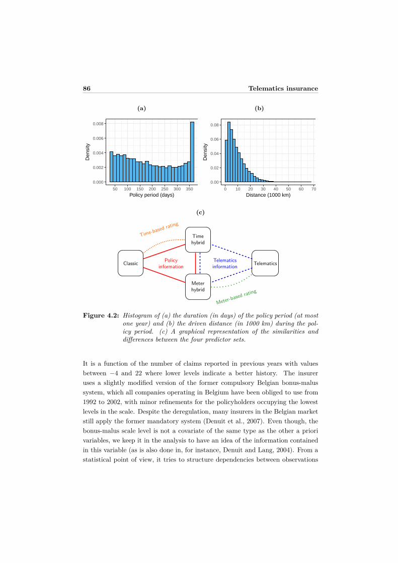
86 Telematics insurance
(a)
0.000
0.002
0.004
0.006
0.008
50 100 150 200 250 300 350
Policy period (days)
Den
sity
(b)
0.00
0.02
0.04
0.06
0.08
0 10 20 30 40 50 60 70
Distance (1000 km)
Den
sity
(c)
Classic
Timehybrid
Meterhybrid
TelematicsPolicyinformation
Telematicsinformation
Time-based rating
Meter-based rating
Figure 4.2: Histogram of (a) the duration (in days) of the policy period (at mostone year) and (b) the driven distance (in 1000 km) during the pol-icy period. (c) A graphical representation of the similarities anddifferences between the four predictor sets.
It is a function of the number of claims reported in previous years with valuesbetween −4 and 22 where lower levels indicate a better history. The insureruses a slightly modified version of the former compulsory Belgian bonus-malussystem, which all companies operating in Belgium have been obliged to use from1992 to 2002, with minor refinements for the policyholders occupying the lowestlevels in the scale. Despite the deregulation, many insurers in the Belgian marketstill apply the former mandatory system (Denuit et al., 2007). Even though, thebonus-malus scale level is not a covariate of the same type as the other a priorivariables, we keep it in the analysis to have an idea of the information containedin this variable (as is also done in, for instance, Denuit and Lang, 2004). From astatistical point of view, it tries to structure dependencies between observations
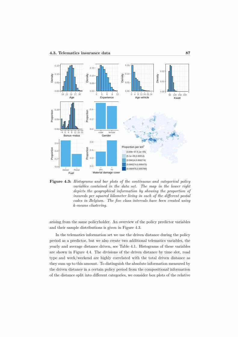
4.3. Telematics insurance data 87
0.00
0.05
0.10
0.15
18 21 24 27 30
Age
Den
sity
0.00
0.05
0.10
0.15
0 3 6 9 12
Experience
Den
sity
0.00
0.05
0.10
0.15
0 4 8 12 16 20 24
Age vehicle
Den
sity
0.00
0.01
0.02
50 100 150 200
Kwatt
Den
sity
0.00
0.05
0.10
−4 0 4 8 12 16 20
Bonus−malus
Pro
port
ion
0.0
0.2
0.4
male female
Gender
Pro
port
ion
0.0
0.2
0.4
0.6
Diesel Petrol
Fuel
Pro
port
ion
0.0
0.2
0.4
0.6
yes no
Material damage cover
Pro
port
ion Proportion per km2
[3.69e−07,5.1e−05)
[5.1e−05,0.00014)
[0.00014,0.000274)
[0.000274,0.000475)
[0.000475,0.000789)
Figure 4.3: Histograms and bar plots of the continuous and categorical policyvariables contained in the data set. The map in the lower rightdepicts the geographical information by showing the proportion ofinsureds per squared kilometer living in each of the different postalcodes in Belgium. The five class intervals have been created usingk-means clustering.
arising from the same policyholder. An overview of the policy predictor variablesand their sample distributions is given in Figure 4.3.
In the telematics information set we use the driven distance during the policyperiod as a predictor, but we also create two additional telematics variables, theyearly and average distance driven, see Table 4.1. Histograms of these variablesare shown in Figure 4.4. The divisions of the driven distance by time slot, roadtype and week/weekend are highly correlated with the total driven distance asthey sum up to this amount. To distinguish the absolute information measured bythe driven distance in a certain policy period from the compositional informationof the distance split into different categories, we consider box plots of the relative
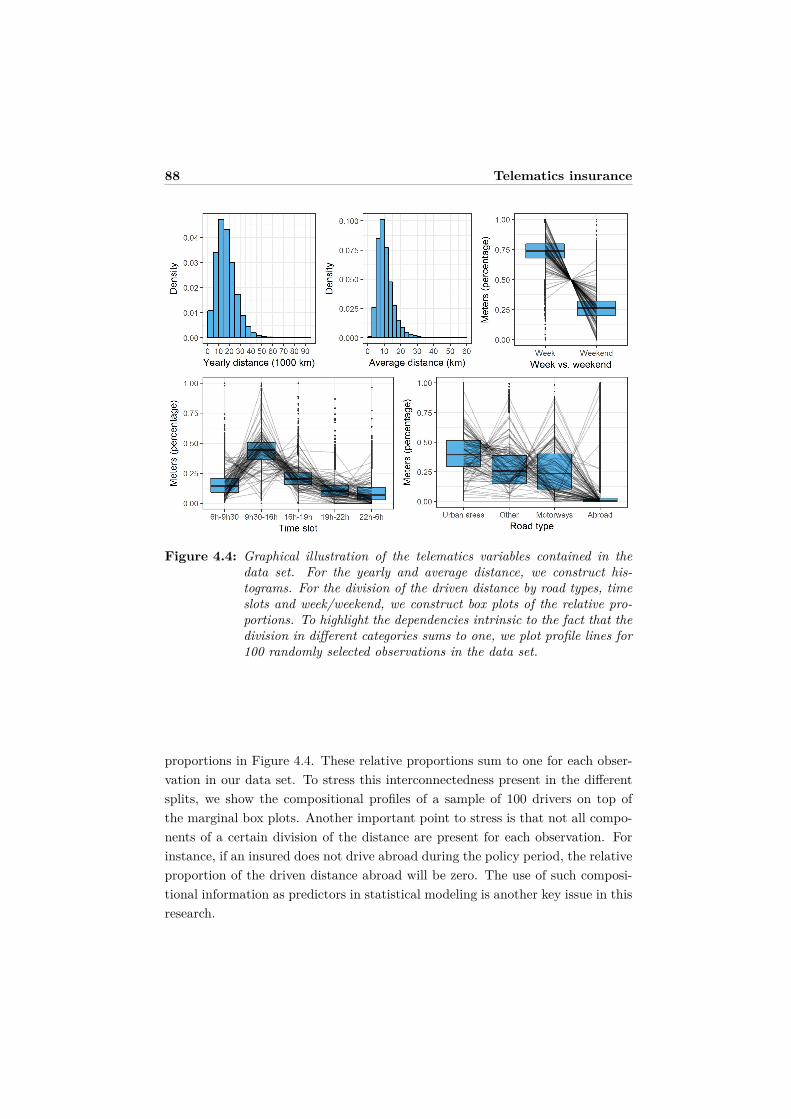
88 Telematics insurance
Figure 4.4: Graphical illustration of the telematics variables contained in thedata set. For the yearly and average distance, we construct his-tograms. For the division of the driven distance by road types, timeslots and week/weekend, we construct box plots of the relative pro-portions. To highlight the dependencies intrinsic to the fact that thedivision in different categories sums to one, we plot profile lines for100 randomly selected observations in the data set.
proportions in Figure 4.4. These relative proportions sum to one for each obser-vation in our data set. To stress this interconnectedness present in the differentsplits, we show the compositional profiles of a sample of 100 drivers on top ofthe marginal box plots. Another important point to stress is that not all compo-nents of a certain division of the distance are present for each observation. Forinstance, if an insured does not drive abroad during the policy period, the relativeproportion of the driven distance abroad will be zero. The use of such composi-tional information as predictors in statistical modeling is another key issue in thisresearch.
4.4. Model building and selection 89
4.4 Model building and selection
We model the frequencies of claims by constructing Poisson and negative binomial(NB) regression models. We denote by Nit the number of claims for policyholderi in policy period t with i = 1, . . . , I and t = 1, . . . , Ti. The model is denotedby Nit ∼ Poisson(µit) or Nit ∼ NB(µit, φ), where µit = E(Nit) represents theexpected number of claims reported by policyholder i in policy period t andφ is the parameter of the NB distribution such that Var(Nit) = µit + µ2
it/φ,allowing for overdisperion. A log linear relationship between the mean and thepredictor variables is specified by the log link function. This means that weset µit = exp(ηit) where ηit is a predictor function of the available explanatoryfactors. The probability mass functions for the Poisson and the NB models are,respectively, expressed as
P(Nit = nit) = exp(−µit)µnitit
nit!and P(Nit = nit) = Γ(φ + nit)
nit!Γ(φ)φφµnit
it
(φ + µit)φ+nit.
For each of the predictor sets in Figure 4.2c we construct the best model using theallowed information based on AIC, see Section 4.4.3. Additionally, we identify thebest models under the restriction that the risk is proportional to the time or meterexposure. This is accomplished by incorporating the logarithm of the exposure-to-risk, either duration of the policy period or total distance driven during thepolicy period, as an offset term in the predictor, i.e. a regression variable witha constant coefficient of 1 for each observation. In the most general case, thepredictor has the form
ηit = β0 + offset + ηcatit + ηcont
it + ηspatialit + ηre
it + ηcompit , (4.1)
where β0 denotes the intercept, the categorical effects are bundled in ηcatit , the
term ηcontit contains the effects of the continuous predictors, ηspatial
it represents thegeographical effect, ηre
it the policyholder-specific random effect and the term ηcompit
embodies the effects of the compositional predictors. Under the offset restriction,the continuous effect of the exposure-to-risk, either the duration of the policy pe-riod (time based rating) or the driven distance (meter based rating), gets replacedby the logarithm of the exposure-to-risk as an offset.
Zero inflated variants of these models could also be considered but is not donehere for interpretability reasons since they are not able to capture the effect of avarying exposure-to-risk in a transparent and intuitive way.
90 Telematics insurance
4.4.1 Generalized additive models
The model framework we work with in this study is the one of generalized addi-tive models (GAMs), introduced by Hastie and Tibshirani (1986). GAMs allowto incorporate continuous covariates in a more flexible way as compared to thetraditional GLMs used in actuarial practice (see e.g. Klein et al., 2014). Froman accuracy standpoint, GAMs are competitive with popular black box machinelearning techniques (such as neural networks, random forests or support vectormachines), but they have the important advantage of interpretability. In insur-ance pricing it is of crucial importance to have interpretable results in order tounderstand the premium structure and explain this to clients and regulators.Using a semiparametric additive structure, GAMs define nonparametric relation-ships between the response and the continuous predictors in the predictor in thefollowing way
ηcatit + ηcont
it = Zitβ +J∑
j=1fj(xjit) ,
where Zit represents the row corresponding to policyholder i in policy periodt of the model matrix of parametric terms for the categorical predictors withparameter vector β and fj represents a smooth function of the jth continuouspredictor variable. To estimate fj , we choose cubic spline basis functions Bjk,such that fj can be represented as fj(x) =
∑qk=1 γjkBjk(x). The knots are chosen
using 10 quantiles of the unique xj values. Cardinal basis functions parametrizethe spline in terms of its values at the knots (Lancaster and Salkauskas, 1986). Foridentifiability, we impose constraints by centering each smooth component aroundzero, thus
∑Ii=1∑Ti
t=1 fj(xjit) = 0 for j = 1, . . . , J. To avoid overfitting, the cubicsplines are penalized by the integrated squared second derivative (Green andSilverman, 1994), which yields a measure for the overall curvature of the function.For each component, this penalty can be written as a quadratic function,∫ (
f ′′j (x)
)2dx =
q∑k=1
q∑l=1
γjkγjl
∫B′′
jk(x)B′′jl(x)dx = γt
jSjγj ,
with (Sj)kl =∫
B′′jk(x)B′′
jl(x)dx. Given these penalty functions for each compo-nent, we define the penalized log-likelihood as
`(ψ)− 12
J∑j=1
λjγtjSjγj , (4.2)
4.4. Model building and selection 91
where `(ψ) denotes the log-likelihood as a function of all model parametersψ = (β,γ1, . . . ,γJ)t and λj denotes the smoothness parameter that controlsthe tradeoff between goodness of fit and the degree of smoothness of componentfj for j = 1, . . . , J . Different smoothing parameters for each component allow topenalize the smooth functions differently.
The model parameters ψ are estimated by maximizing (4.2) using penalizediteratively reweighted least squares (P–IRLS) (Wood, 2006). For the Poissonmodel, the smoothing parameters λ1, . . . , λJ are estimated using an unbiased riskestimator criterion (UBRE), which is a rescaled version of Akaike’s informationcriterion (AIC; Akaike, 1974). For the negative binomial model, we estimatethe smoothing parameters and the scale parameter φ using maximum likelihood(ML).
In addition to categorical and continuous covariates, the data set contains spa-tial information, namely the postal code where the policyholder resides. Insurancecompanies tend to use the geographical information of the insured’s residence asa proxy for the traffic density and for other unobserved socio-demographic factorsof the neighborhood. We model the spatial heterogeneity of claim frequencies byadding a spatial term ηspatial
it = fs(latit, longit) in the additive predictor ηit, us-ing the latitude and longitude coordinates (in degrees) of the center of the postalcode where the policyholder resides. We use second order smoothing splines onthe sphere (Wahba, 1981) to model fs. This allows us to quantify the effect of thegeographic location while taking the regional closeness of the neighboring postalcodes into account.
In our data set, many policyholders i = 1, . . . , I are observed over multiplepolicy periods t = 1, . . . , Ti. This longitudinal aspect of the data can be modeledby including policyholder-specific random effects ηre
it in the predictor. The gen-eralized additive model considered thus far is extended in this way by exploitingthe link between penalized estimation and random effects (see e.g. Ruppert et al.,2003). We assess whether such random effects are needed to take the correlationsbetween observations of the same policyholder into account using the approximatetest for a zero random effect developed by Wood (2013).
4.4.2 Compositional data
The divisions of the total driven distance in the different categories – road types(4), time slots (5) and week/weekend (2), see Table 4.1 – are highly correlatedwith and sum up to the total driven distance. Incorporating these divisions in

92 Telematics insurance
a predictor also containing the total distance leads to a perfect multicollinearityproblem. Furthermore, the corresponding model parameter estimators are not in-variant to the ordering of the components: the statistical inference changes whenpermuting the components making interpretations misleading. The standard re-gression interpretation of a change in one of the components of the distance whenthe other components are held constant is not possible due to the sum constraintof adding up to the total distance.
The total distance in meters is used as a continuous predictor in the telematicsmodels and its effect is modeled using a smooth function. Since the divisions of thedistance only contribute additional relative information, we divide all componentsof each split by the total driven distance, see Figure 4.4. We obtain what isknown as compositional data (Van den Boogaart and Tolosana-Delgado, 2013;Pawlowsky-Glahn et al., 2015). Such data are represented by real vectors withconstant sum equal to one and positive components. The space of representationsof compositions is called the simplex of D parts, denoted SD, defined by
SD ={x = (x1, . . . , xD)t : xi > 0,
D∑i=1
xi = 1}
.
Only relative information is important, and multiplication of the vector of pos-itive components by a positive constant does not change the ratios between thecomponents. When data are considered compositional, classical statistics, thatdo not take the special geometry of the simplex into account, are not appropri-ate. Extending the current literature, we propose a new way of quantifying andinterpreting the effect of the compositional explanatory variables on the outcomeand propose an approach to deal with structural zeros.
The Aitchison geometry of the simplex
The vector space structure of the mathematical simplex was discovered by Aitchi-son (1986) who defined operations on compositional data leading to the Aitchisongeometry of the simplex. Perturbation plays the role of addition on the simplexand is defined as a closed component-wise product x ⊕ y = C(x1y1, . . . , xDyD)t,where the closing operation C ensures a total sum of one, i.e. the closure of x isC(x) = x/
∑Di=1 xi. The product of a vector by a scalar is called powering and is
defined as α � x = C(xα1 , . . . , xα
D)t, for α ∈ R. The Aitchison inner product for
4.4. Model building and selection 93
compositions is
〈x,y〉a = 12D
D∑i=1
D∑j=1
ln xi
xjln yi
yj=
D∑i=1
ln(xi) ln(yi)−1D
(D∑
i=1ln(xi)
) D∑j=1
ln(yj)
and induces the following norm ‖x‖a =
√〈x,x〉a and distance da(x,y) = ‖x
y‖a, where represents the opposite operation of ⊕, i.e. y = ⊕((−1)�y). Thesimplex along with these operations then forms a (D − 1)-dimensional Euclideanvector space (SD,⊕,�, 〈·, ·〉a). Given this Euclidean structure, we can measuredistances and angles, and define related geometrical concepts. Elementary sta-tistical notions involving the metrics of the sample space can be adapted to theEuclidean structure of the simplex.
Egozcue et al. (2003) constructed orthonormal bases for this Euclidean spaceand deduced corresponding isometries between SD and RD−1, called isometriclogratio transformations (ilr). One possible ilr transformation maps a composi-tional data vector x in a (D − 1)-dimensional real vector z = (z1, z2, . . . , zD−1)t
with components
zi = ilri(x) =√
D − i
D − i + 1 ln xi
D−i
√∏Dj=i+1 xj
, i = 1, . . . , D − 1 . (4.3)
As the ilr transformation is isometric, all angles and distances are preserved. Thismeans that, whenever compositions are transformed into coordinates, the metricsand operations in the Aitchison geometry of the simplex are translated into theordinary Euclidean metrics and operations in real space. Let V be the D×(D−1)matrix with elements
Vij = D − j√(D − j + 1)(D − j)
for i = j,−1√
(D − j + 1)(D − j)for i > j,
and 0 otherwise, for which it holds that V tV = ID−1 and V V t = ID−(1/D)1D1tD,
where ID is the identity matrix of dimension D and 1D a D-vector of ones(Egozcue et al., 2011). Then we can rewrite this ilr transform and its inversein matrix notation as
z = ilr(x) = V t lnx , and x = ilr−1(z) = C(exp(V z)) , (4.4)
where the logarithmic and exponential function apply componentwise.
94 Telematics insurance
Even though the simplex SD is a subset of the real space RD, Aitchison (1986)showed that the geometry is clearly different. Ignoring this aspect in a statisticalcontext can lead to incompatible or incoherent results. The compositional na-ture of the data must not be ignored. The principle of working on coordinatesin statistics (Mateu-Figueras et al., 2011) is to first express the compositionaldata with respect to an orthonormal basis of the underlying vector space withEuclidean structure. Next, to apply standard statistical techniques to the vectorsof coordinates and, finally, to back-transform and describe the results in terms ofthe simplex. Final results do not depend on the chosen basis.
A new interpretation for compositional predictors
In our setting, it is key to incorporate the compositional data arising from thedivisions of the distances into different categories as predictors in the claim countregression models. Hron et al. (2012) propose to first apply the isometric logratio transform (4.3) to map the compositions in the D-part Aitchison simplex toa (D − 1) Euclidean space. Then, these terms are used as explanatory variablesin a linear regression model. More generally, in any regression context involv-ing a predictor, one can add a compositional predictor term ηcomp using the ilrtransformed variables, i.e.
ηcomp = β1z1 + . . . + βD−1zD−1 . (4.5)
The fitted model does not depend on the choice of the orthonormal ilr basis sincethe coordinates of x with respect to different orthonormal bases are orthogonaltransformations of each other. Using the ilr transformation the model parameterscan be estimated without constraints and the ceteris paribus interpretation ofaltering one zi without altering any other becomes possible. Only the first regres-sion parameter, β1, however has a comprehensible interpretation since z1 explainsrelevant information about x1. The remaining coefficients are not straightforwardto interpret and hence Hron et al. (2012) suggest to permute the indices in formula(4.3) and construct D regression models, each time with a different componentfirst for which we can interpret the corresponding coefficient. Having to refit themodel multiple times is undesirable, especially in our case where we have morethan one compositional predictor and each model fit is computationally intensivedue to smooth continuous, spatial, and random effects. Hence, we develop a newstrategy to include compositional predictors and interpret their effect.
By using the inverse ilr transform on the model coefficients, i.e. set b = ilr−1(β)
4.4. Model building and selection 95
where β = (β1, . . . , βD−1)t, we can rewrite the compositional predictor as
ηcomp =D−1∑i=1
βizi =D−1∑i=1
ilri(b)ilri(x) = 〈b,x〉a ,
since the ilr transform preserves the inner product (Van den Boogaart and Tolosana-Delgado, 2013; Pawlowsky-Glahn et al., 2015). The composition b ∈ SD can beinterpreted as the simplicial gradient of ηcomp with respect to x (Barcelo-Vidalet al., 2011) and is the compositional direction along which the predictor increasesfastest. In particular, if we increase x to x = x⊕ b
‖b‖a, then the predictor becomes
ηcomp = 〈b, x〉a = 〈b,x⊕ b
‖b‖a〉a = 〈b,x〉a + 1
‖b‖a〈b, b〉a = ηcomp + ‖b‖a .
When D = 3, the estimated regression model can be visualized as a surface on aternary diagram (Van den Boogaart and Tolosana-Delgado, 2013). For D > 3, agraphical representation is not straightforward.
In order to overcome this shortcoming in interpretation and to develop a graph-ical representation for compositional explanatory variables, we propose to perturbthe composition in the direction of each component. This offers a new interpre-tation for the effect of altering the composition on the predictor. For example,a relative ratio change of α > 1 (increase) or α < 1 (decrease) in the first com-ponent of x with constant ratios of the remaining components can be achievedby perturbing the composition x by (α, 1, . . . , 1)t. This leads to a change of thepredictor given by
〈b, (α, 1, . . . , 1)t〉a = ln(b1) ln(α)− 1D
(D∑
i=1ln(bi)
)ln(α) = clr1(b) ln(α) , (4.6)
which is independent of the original composition x and where
clri(b) = ln(
bi
gm(b)
), gm(b) =
(D∏
i=1bi
)1/D
, i = 1, . . . , D
denotes the centered log-ratio (clr) transform of b (Egozcue et al., 2011). Theeffect of a relative increase in any of the components can hence best be un-derstood by considering the clr transform of b, of which the elements sum tozero and indicate the positive or negative effect of each component on the pre-dictor. A graphical representation of the effect of a compositional predictor
96 Telematics insurance
can be made by visualizing clr(b) and comparing the elements to zero. Sinceβ = ilr(b) = V t ln(b) = V tclr(b) and V V t = ID − (1/D)1D1t
D, the clr transformof b can be written as clr(b) = V β. Confidence bounds can thus be constructedusing the corresponding covariance matrix V ΣV t where Σ is the estimated co-variance matrix related to estimating β. To interpret the effect on the level of theexpected outcome in the Poisson and NB models, we can transform these confi-dence intervals using the exponential function. The exponentiated clr transformof b has to be compared to one and the effect of a relative ratio change of α incomponent i = 1, . . . , D is given by αclri(b).
Dealing with structural zeros in compositional predictors
An additional difficulty when incorporating the compositional information as pre-dictors in the analysis of the claim counts is the presence of proportions of a spe-cific component that are exactly zero. In the division of the driven distance byroad type, for instance, many insureds did not drive abroad during the observedpolicy period. Since compositional data are always analyzed by considering lo-gratios of the components (see Section 4.4.2), a workaround is necessary.
In the compositional data literature, different types of zeros are being dis-tinguished (Pawlowsky-Glahn et al., 2015). Rounded zeros occur when certaincomponents may be unobserved because their true values are below the detec-tion limit (cfr. geochemical studies). Count zeros refer to zero values due to thelimited size of the sample in compositional data arising from count data. In oursetting, the zero values are truly zero and are not due to imprecise or insufficientmeasurements. Such kind of zeros are called structural zeros. The structural ze-ros patterns in the data set are listed in Appendix 4.7. The presence of zerosis most prominent for splitting distance by road types as 40% of the drivers didnot go abroad. Zeros are most often dealt with using replacement strategies (seee.g. Martın-Fernandez et al., 2011, for an overview), which do not make sense forstructural zeros. A general methodology is still to be developed (see e.g. Aitchisonand Kay, 2003; Bacon Shone, 2003). In particular, there does not exist a methodthat deals with compositional data with structural zeros as predictor in regressionmodels. Applying the ilr transform to the compositional data x and using thetransformed z as explanatory variables in the predictor as discussed in Section4.4.2 is no longer possible.
We propose to treat the structural zero patterns of the compositional predic-tors as different subgroups within the data and model the effect conditional onthe zero pattern. In the most general situation, 2D − 1 possible zero patterns can
4.4. Model building and selection 97
occur when dealing with compositional data with D components (a structuralzero for every component being excluded). We introduce indicator variables foreach zero pattern and use these in the compositional predictor term ηcomp of theregression model to specify the effect on the outcome separately for each zeropattern. More specifically, we define the variables
d(i1,...,ik) =
1 if components i1, . . . , ik of x are nonzero and all other are zero ,
0 otherwise
for all k = 1, . . . , D and 1 6 i1 < . . . < ik 6 D. Conditional on the zero pattern(i1, . . . , ik) of the compositional data vector x, the contribution to the predictoris given by the Aitchison inner product 〈b(i1,...,ik),x(i1,...,ik)〉a of the subcompo-sition x(i1,...,ik) existing of the nonzero components of x and a subcompositionalsimplicial gradient b(i1,...,ik), which is different for each zero pattern. In case ofonly one nonzero component, the contribution is given by a simple categorical ef-fect b(i). Note that the subscript (i1, . . . , ik) has a different interpretation for thedummy variable, simplicial gradient and compositional data vector. The proposedcompositional predictor reads
ηcomp =D∑
i=1d(i)b(i) +
D∑k=2
∑16i1<...<ik6D
d(i1,...,ik)〈b(i1,...,ik),x(i1,...,ik)〉a .
Zero pattern specific intercepts can be added in the second term if deemed nec-essary.
4.4.3 Model selection and assessment
Using the same form as Akaike’s information criterion, AIC for a GAM is definedas
AIC = −2 · + 2 · EDF (4.7)
where is the log-likelihood, evaluated at the estimated model parameters ob-tained using penalized likelihood maximization, and the effective degrees of free-dom (EDF) is used instead of the actual number of model parameters. The EDF isdefined as the trace of the hat or smoothing matrix in the corresponding workinglinear model at the last P-IRLS iteration (Hastie and Tibshirani, 1990). As such,(4.7) measures the quality of the model as a trade-off between the goodness-of-fitand the model complexity.
98 Telematics insurance
For each of the four predictor sets, see Figure 4.2c, variables are selected byAIC using an exhaustive search over all the possible combinations of variablesgiven in Table 4.1. We limit ourselves to additive regression models (i.e. nointeractions) such that an exhaustive search is still feasible and the marginalimpact of a single variable can be easily assessed, interpreted and visualized.Even though the 2011 EU ruling prohibits a distinction between men and womenin car insurance pricing, we allow gender to be selected as a categorical predictorin the model. For the division of the number of meters in different categories,10 structural zero patterns occur for the road types, 20 for the time slots, and3 for week/weekend. However, based on their relative frequencies, we only allowan additional compositional predictor for the distinction by road type in the casethat a car did not drive abroad, which occurs for 40% of the observations. Allremaining zero patterns are bundled into one residual group and their effect ismodeled using a categorical effect b0, see Table 4.8 of Appendix 4.7. The mostcomprehensive compositional predictor term we allow to be selected in the hybridand telematics models is
ηcompit = droad
(1111)〈broad(1111),x(1111)〉a + droad
(1110)〈broad(1110),x(1110)〉a
+(1− droad(1111) − droad
(1110))broad0 + dtime
(11111)〈btime(11111),x(11111)〉a
+(1− dtime(11111))btime
0 + dweek(11) 〈b
week(11) ,x(11)〉a + (1− dweek
(11) )bweek0 .
In total, 165 888 model specifications are estimated under both the Poisson andthe negative binomial framework.
Predictive performance of these models is assessed using proper scoring rulesfor count data, see Table 4.2 (Czado et al., 2009). Scoring rules assess the qualityof probabilistic forecasts through a numerical score s(P, n) based on the predictivedistribution P and the observed count n. Lower scores indicate a better qualityof the forecast. A scoring rule is proper (Gneiting and Raftery, 2007) if s(Q, Q) 6s(P, Q) for all P and Q with s(P, Q) the expected value of s(P, ·) under Q. Ingeneral, we define by pk = P(N = k) and Pk = P(N 6 k) the probability massfunction and cumulative probability function of the predictive distribution P forcount variable N . The probability mass at the observed count n is denoted as pn.The mean and standard deviation of P are written as µP and σP , respectively,and we set ‖p‖ =
∑∞k=0 p2
k.We compare the predictive performance of the best models according to AIC
under the four predictor sets, with or without offset in the predictor (4.1), andusing a Poisson or negative binomial distribution. We apply the proper scoring
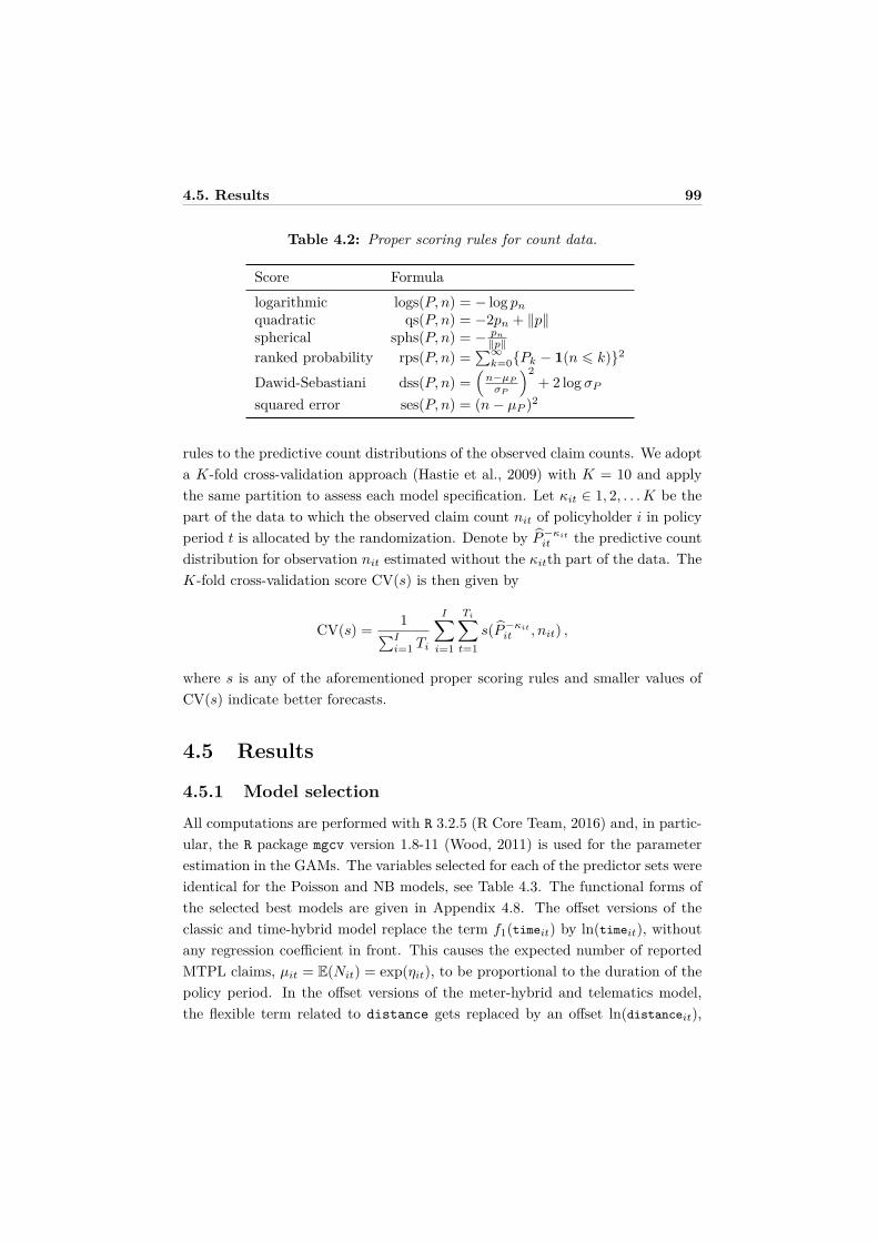
4.5. Results 99
Table 4.2: Proper scoring rules for count data.
Score Formulalogarithmic logs(P, n) = − log pn
quadratic qs(P, n) = −2pn + ‖p‖spherical sphs(P, n) = − pn
‖p‖ranked probability rps(P, n) =
∑∞k=0{Pk − 1(n 6 k)}2
Dawid-Sebastiani dss(P, n) =(
n−µP
σP
)2+ 2 log σP
squared error ses(P, n) = (n− µP )2
rules to the predictive count distributions of the observed claim counts. We adopta K-fold cross-validation approach (Hastie et al., 2009) with K = 10 and applythe same partition to assess each model specification. Let κit ∈ 1, 2, . . . K be thepart of the data to which the observed claim count nit of policyholder i in policyperiod t is allocated by the randomization. Denote by P −κit
it the predictive countdistribution for observation nit estimated without the κitth part of the data. TheK-fold cross-validation score CV(s) is then given by
CV(s) = 1∑Ii=1 Ti
I∑i=1
Ti∑t=1
s(P −κitit , nit) ,
where s is any of the aforementioned proper scoring rules and smaller values ofCV(s) indicate better forecasts.
4.5 Results
4.5.1 Model selection
All computations are performed with R 3.2.5 (R Core Team, 2016) and, in partic-ular, the R package mgcv version 1.8-11 (Wood, 2011) is used for the parameterestimation in the GAMs. The variables selected for each of the predictor sets wereidentical for the Poisson and NB models, see Table 4.3. The functional forms ofthe selected best models are given in Appendix 4.8. The offset versions of theclassic and time-hybrid model replace the term f1(timeit) by ln(timeit), withoutany regression coefficient in front. This causes the expected number of reportedMTPL claims, µit = E(Nit) = exp(ηit), to be proportional to the duration of thepolicy period. In the offset versions of the meter-hybrid and telematics model,the flexible term related to distance gets replaced by an offset ln(distanceit),
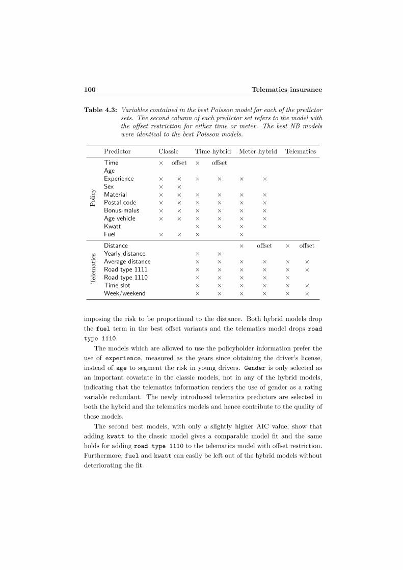
100 Telematics insurance
Table 4.3: Variables contained in the best Poisson model for each of the predictorsets. The second column of each predictor set refers to the model withthe offset restriction for either time or meter. The best NB modelswere identical to the best Poisson models.
Predictor Classic Time-hybrid Meter-hybrid Telematics
Polic
y
Time × offset × offsetAgeExperience × × × × × ×Sex × ×Material × × × × × ×Postal code × × × × × ×Bonus-malus × × × × × ×Age vehicle × × × × × ×Kwatt × × × ×Fuel × × × ×
Tele
mat
ics
Distance × offset × offsetYearly distance × ×Average distance × × × × × ×Road type 1111 × × × × × ×Road type 1110 × × × × ×Time slot × × × × × ×Week/weekend × × × × × ×
imposing the risk to be proportional to the distance. Both hybrid models dropthe fuel term in the best offset variants and the telematics model drops roadtype 1110.
The models which are allowed to use the policyholder information prefer theuse of experience, measured as the years since obtaining the driver’s license,instead of age to segment the risk in young drivers. Gender is only selected asan important covariate in the classic models, not in any of the hybrid models,indicating that the telematics information renders the use of gender as a ratingvariable redundant. The newly introduced telematics predictors are selected inboth the hybrid and the telematics models and hence contribute to the quality ofthese models.
The second best models, with only a slightly higher AIC value, show thatadding kwatt to the classic model gives a comparable model fit and the sameholds for adding road type 1110 to the telematics model with offset restriction.Furthermore, fuel and kwatt can easily be left out of the hybrid models withoutdeteriorating the fit.
4.5. Results 101
For each of these best model formulations, we added a policyholder-specificrandom effect in the predictor (4.1) to account for possible dependence from ob-serving policyholders over multiple policy periods. However, none of the addedrandom effects were deemed necessary at the 5% significance level using the ap-proximate test of Wood (2013).
4.5.2 Model assessment
Table 4.4 reports AIC and all 6 proper scoring rules obtained using 10-fold crossvalidation for each predictor set under the Poisson model specification. These per-formance tools unanimously indicate that the time-hybrid model without offsetscores best. The meter-hybrid model is a close second. Their respective ver-sions with an offset restriction and the telematics model without offset concludethe top five according to all criteria except the Dawid–Sebastiani score. Thisdemonstrates the significant impact of telematics constructed variables on thepredictive power of the model. In addition, the telematics model without offsetoutperforms the classic models across all assessment criteria. Hence, using onlytelematics predictors is considered to be better than the use of the traditionalrating variables.
Across all predictor sets, the use of an offset for the exposure-to-risk, eithertime or meter, is too restrictive for these data. From a statistical point of view,the time or meter rating unit cannot be considered to be directly proportional tothe risk. However, from a business point of view, it is convenient to consider aproportional approach due to its simplicity and explainability.
Similar results are obtained under the negative binomial model specification.The rankings according to AIC are the same as in Table 4.4. The AIC values foreach predictor set under the NB model specification compared to their Poissoncounterpart were slightly higher for the classic and hybrid models and slightlylower for the telematics models indicating that only the telematics predictor setsbenefit from the additional parameter to capture overdispersion. The model as-sessment using proper scoring rules led to the same conclusions as before.
Beside an exhaustive search among additive terms, we have explored the use ofinteractions among categorical, among continuous, between categorical and con-tinuous, and between categorical and compositional predictors. Slight marginalimprovements in AIC could only be achieved in the classic model by further re-fining the effects of experience, age vehicle and material by gender withoutchanging the rankings in Table 4.4 of the best models.
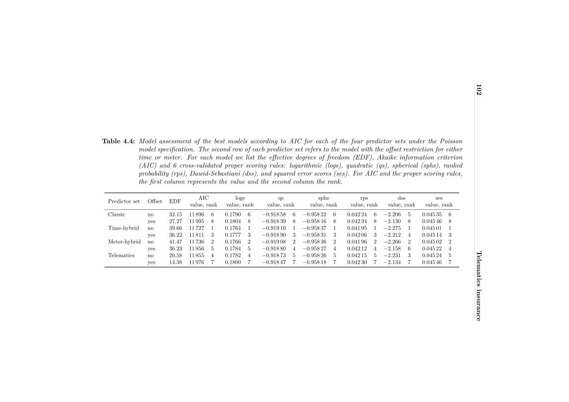
102T
elematics
insurance
Table 4.4: Model assessment of the best models according to AIC for each of the four predictor sets under the Poissonmodel specification. The second row of each predictor set refers to the model with the offset restriction for eithertime or meter. For each model we list the effective degrees of freedom (EDF), Akaike information criterion(AIC) and 6 cross-validated proper scoring rules: logarithmic (logs), quadratic (qs), spherical (sphs), rankedprobability (rps), Dawid-Sebastiani (dss), and squared error scores (ses). For AIC and the proper scoring rules,the first column represents the value and the second column the rank.
Predictor set Offset EDF AIC logs qs sphs rps dss sesvalue, rank value, rank value, rank value, rank value, rank value, rank value, rank
Classic no 32.15 11 896 6 0.1790 6 −0.918 58 6 −0.958 22 6 0.042 24 6 −2.206 5 0.045 35 6yes 27.27 11 995 8 0.1804 8 −0.918 39 8 −0.958 16 8 0.042 34 8 −2.130 8 0.045 46 8
Time-hybrid no 39.66 11 727 1 0.1764 1 −0.919 10 1 −0.958 37 1 0.041 95 1 −2.275 1 0.045 01 1yes 36.22 11 811 3 0.1777 3 −0.918 90 3 −0.958 31 3 0.042 06 3 −2.212 4 0.045 14 3
Meter-hybrid no 41.47 11 736 2 0.1766 2 −0.919 08 2 −0.958 36 2 0.041 96 2 −2.266 2 0.045 02 2yes 36.23 11 856 5 0.1784 5 −0.918 80 4 −0.958 27 4 0.042 12 4 −2.158 6 0.045 22 4
Telematics no 20.58 11 855 4 0.1782 4 −0.918 73 5 −0.958 26 5 0.042 15 5 −2.231 3 0.045 24 5yes 14.38 11 976 7 0.1800 7 −0.918 47 7 −0.958 18 7 0.042 30 7 −2.134 7 0.045 46 7
4.5. Results 103
4.5.3 Visualization and discussion
The effects of each predictor variable in the best time-hybrid model without off-set restriction are graphically displayed in Figure 4.5 for the policy model termsand Figure 4.6 for the telematics model terms. By exponentially transformingthe additive effects, we show the multiplicative effects on the expected number ofclaims for each categorical parametric, continuous smooth or geographical termin the fitted model. For the categorical predictors we quantify the uncertaintyof those estimates by constructing individual 95% confidence intervals based onthe large sample normality of the model parameter estimators. Bayesian 95%confidence pointwise intervals are used for the smooth components of the GAMand include the uncertainty about the intercept (Marra and Wood, 2012). For thecompositional data predictors, we visualize the exponentiated clr transform of thecorresponding model parameters with 95% confidence intervals along with a ref-erence line at one (see Section 4.4.2). Similar graphs for the other three predictorsets, see Figure 4.2c, are shown in Appendix 4.9 and the relative importance ofthese predictors is quantified and visualized in Appendix 4.10. In the remainderof this section, we discuss the insights and interpretations for both the policy andtelematics variables in each of these models.
Policy variables The rating unit policy period in the classic and time-hybridmodels always has a monotone increasing estimated effect. The longer a policy-holder is insured, the higher the premium amount, ceteris paribus. Using the factthat the level of the nonlinear smooth components are not uniquely identifiable(see Section 4.4.1), we vertically translated the estimated smooth term to passthe point (365, 0) on the predictor scale (and hence (365, 1) on the response scale)for ease of interpretation.
The smooth effect of experience embodies the higher risk posed by younger,less experienced drivers. The increased risk is more outspoken in the first twoyears for the hybrid models as compared to the classic model.
In the classic model, the significant effect of gender indicates that womenare 16% less risky drivers than men. However, when telematics predictors aretaken into account in the hybrid models, the categorical variable gender is nolonger selected as predictor. Neither did any interaction term between genderand a categorical, a continuous or a compositional predictor improve AIC. Theperceived difference between women and men can hence be explained throughdifferences in driving habits. In particular, female drivers in the portfolio drivesignificantly fewer kilometers on a yearly basis compared to men (15 409 vs 18 570
104 Telematics insurance
on average, with a p-value smaller than 0.001 using a two sample t-test). Similarfindings are reported in Ayuso et al. (2016a,b). In light of the EU rules on gender-neutral pricing in insurance, this shows how moving towards car insurance ratingbased on individual driving habits and style can resolve possible discriminationof basing the premium on proxies such as gender.
The smooth effects of bonus-malus in the classic and hybrid models are non-linear and somewhat counterintuitive. Given the lack of a lengthy claim historyof the young drivers of this portfolio, the BM level of the insureds are not yetfully developed and stabilized. The majority of the drivers has a bonus-malus(BM) level between 4 and 12 for which the effect on the claim frequency is in-creasing. For the highest BM levels however, the effect is declining, albeit witha high uncertainty due to a lack of observations in this region. Furthermore, theeffect does not decrease for the lowest BM levels. This can be explained by animproper use of the BM scale as marketing tool to attract new customers. Bylowering the initial value of the BM scale, the insurer can reduce the premium apotential new policyholder has to pay.
When it comes to characteristics of the car, insureds driving older vehicleshave an estimated higher risk of accidents. The smooth effect of age vehicle isestimated as a straight line on the predictor scale in the classic and hybrid models.The effect of kwatt in the hybrid models also reduced to a straight line on thepredictor scale. When the insured vehicle has more horsepower, the estimatedexpected claims number is lower, although this effect is of lesser importance forthe model fit as indicated earlier. The categorical model term fuel shows thatvehicles using petrol have an estimated lower risk for accidents compared to diesel.This difference is however smaller and no longer statistically significant in thehybrid models compared to the classic model.
In both the classic and hybrid models, the policies without material damagecover have a 20% lower estimated expected number of claims. This may be ex-plained by the reluctance of some insureds without additional material damagecoverage to report small accidents. Due to bonus-malus mechanisms being inde-pendent of the claim amount, filing a claim leads to premium surcharges whichmay be more disadvantageous for policyholders than for them to defray the thirdparty. This phenomenon is known as the hunger for bonus (Denuit et al., 2007).Insureds with an additional material damage cover are less inclined to do so sincetheir own, first party costs are also covered making it more worthwhile to reporta claim at fault. Including telematics variables in the model does not affect thisdiscrepancy.
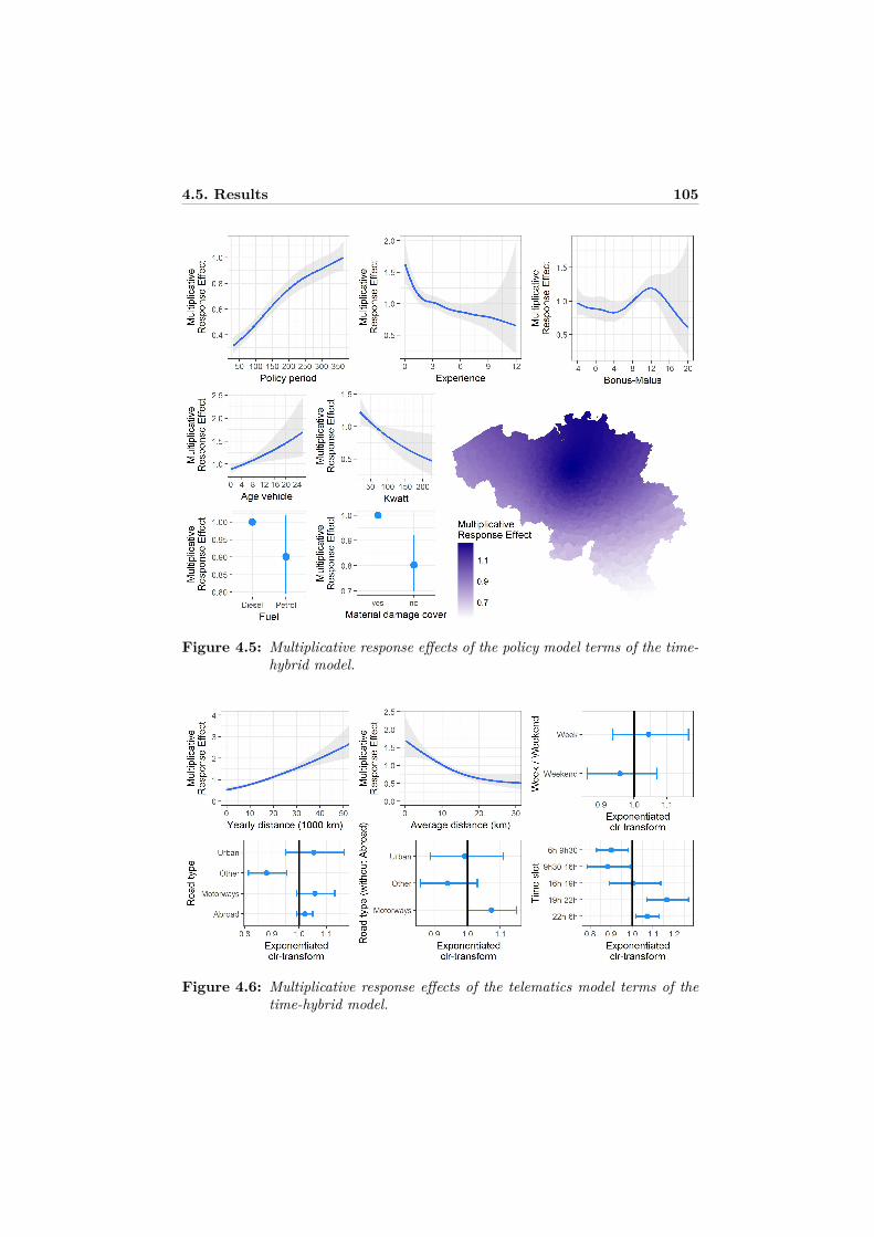
4.5. Results 105
Figure 4.5: Multiplicative response effects of the policy model terms of the time-hybrid model.
Figure 4.6: Multiplicative response effects of the telematics model terms of thetime-hybrid model.
106 Telematics insurance
The geographical effect (postal code), plotted on top of a map of Belgiumfor the classic and hybrid models, captures the remaining spatial heterogeneitybased on the postal code where the policyholder resides. For the classic model,the graph shows higher claim frequencies for urban areas like Brussels in themiddle, Antwerp in the north and Liege in the east and lower claim frequenciesin the more sparsely populated regions in the south. The geographic variationhowever decreases strongly in the hybrid models due to the inclusion of telematicspredictors not taken into account in the classic model. The EDF correspondingto the spatial smooth reduced from 15.8 in the classic model to 6.4 in both hybridmodels. This is satisfactory as it means, instead of overrelying on geographicalproxies, the hybrid models are basing the insurance premium on actual differencesin driving habits (such as the proportion driven on urban roads) which is moreclosely related to the accident risk.
Telematics variables In the meter-hybrid and telematics models, distanceis used as the rating unit. Similar to the time effect in the classic and time-hybrid model, the effect of the risk exposure is estimated as a monotone increasingfunction. The accident risk however does not vanish for insureds who hardly driveany kilometers during the observation period.
The yearly distance is used in the time-hybrid model, which uses time asexposure, to differentiate between drivers who travel many versus few kilometerson a yearly basis. In this way, the driven distance is rescaled on a yearly basis(see Section 4.3.2) and used as an additional risk factor having a weaker effect onthe claim frequency compared to the meter-hybrid and telematics models wheredistance is used a rating unit. In both hybrid models and the telematics model,the estimated average distance effect shows lower claim frequencies for insuredswho on average drive long distances.
The exponentiated clr transforms of the model coefficients related to the com-positional road type predictor in the telematics model show how insureds whodrive relatively more on urban roads have higher claim frequencies and insuredswho drive relative more on the road type ‘other’ have lower claim frequencies.The same interpretation holds for insureds who do not drive abroad during thepolicy period. In the hybrid models, these effects are headed in the same directionwith the exception that motorways is perceived as riskier. The elevated accidentrisk for insureds driving more on urban roads is in line with Paefgen et al. (2014),where the driven distance is divided over ‘highway’, ‘urban’ and ‘extra-urban’road types. The authors however neglect the compositional nature of this predic-
4.6. Conclusion 107
tor in the analysis and do not incorporate any of the classical policy risk factorsin the logistic regression model. In Ayuso et al. (2014), the percentage of urbandriving is considered an important variable to predict either the time or the dis-tance to the first accident, although percentages driven on different road typesare not considered. Using either a quadratic effect or a categorical effect (urbandriving > 25%) in Weibull regression models shows how increased percentages ofurban driving reduce both the expected time or distance to the first accident.
The compositional time slot predictor in the hybrid and telematics modelsindicates that policyholders who drive relatively more in the morning have lowerclaim frequencies and policyholders who drive relatively more in the evening andduring the night have higher claim frequencies. In Paefgen et al. (2014), theaccident risk is considered to be lower during the daytime (between 5 and 18h)compared to the evening (between 18h and 21h), based on the estimated coef-ficients of linear model terms of the log transformed percentages of the drivendistance in these time slots. Ayuso et al. (2014) reports how a higher percentageof driving at night reduces the expected time to a first accident, where the effectis modeled linearly, with no further distinction in time slots.
Driving more in the week than in the weekend increases the probability ofhaving a claim. An increased accident risk in case of more driving in the weekis also found in Paefgen et al. (2014), though they define weekend from Fridayto Sunday. The compositional effect of week/weekend is retained in both hybridmodels as well as the telematics model according to AIC even though it is notstatistically significant. This is due to a highly significant and positive estimatedcategorical effect bweek
0 for the 73 observations with structural zeros belongingto the rest group, see Table 4.8 of Appendix 4.7. These drivers have jointlydriven 58 000 kilometers during a combined insured policy period of 16.5 yearsand reported the remarkably high number of 5 claims.
4.6 Conclusion
Telematics insurance offers new opportunities for insurers to differentiate driversbased on their driving habits and style. By aggregating the telematics data onthe level of the policy period by policyholder and combining it with traditionalpolicy(holder) rating variables, we construct predictive models for the frequencyof MTPL claims at fault. Generalized additive models with a Poisson or negativebinomial response are used to model the effects of predictors in a smooth, yetinterpretive way. The divisions of the driven distance into 4 road types and 5
108 Telematics insurance
time slots forms a challenge from a methodological point of view that has notbeen addressed in the literature. We demonstrate how to include this informationas compositional predictors in the regression and formulate a new way of how tointerpret their effect on the average claim frequency.
Our research reveals the significant impact of the use of telematics data throughan exhaustive model selection and an assessment of the predictive performance.The time-hybrid is the best model according to AIC and all proper scoring rules,closely followed by the meter-hybrid model. The model using only telematics vari-ables is ranked higher than the best classic model using only traditional policyinformation.
The compositional predictors show that a further classification of the drivendistance based on the location and the time is relevant. Our contribution indicatesthat driving more on urban roads, in the evening or at night and during theweek contributes to a riskier driving pattern. The best hybrid models highlightthat certain popular pricing factors (gender, fuel, postcode) are indeed proxiesfor the driving habits and part of their predictive power is taken over by thedistance driven and the splits into different categories. Hence, we demonstrateusing careful statistical modeling how the use of telematics variables is an answerto the European regulation on insurance pricing practices that bans the use ofgender as a rating factor.
In the case of multiple insured drivers, it is unclear which characteristics (suchas age, experience and gender) the insurer must use to determine the premium.We proceed, in consultation with the Belgian insurer providing the data, by iden-tifying the driver with the lowest experience as the main driver and use his poli-cyholder information as predictors in the regression for tarification purposes. Inpractice, when a parent adds a child as a driver in the policy, a premium surchargeis often avoided to prevent the policyholder from lapsing. By shifting towardspricing based on telematics information as we do in this research, this tarificationissue becomes less of a problem because the premium will be usage-based.
Pricing using telematics data can be seen as falling in between a priori and aposteriori pricing. The driving habits and style are no traditional a priori vari-ables since they cannot be determined before the policyholder starts to drive.Insurers now reason that available UBI products are only purchased by driverswho consider themselves to be either safe or low-kilometer drivers. This potentialform of positive selection, which could not be quantified based on the studiedportfolio alone, validates an upfront discount on the traditional insurance pre-mium. Based on the telematics data collected over time, insurers can set up a
4.7. Appendix A: Structural zero patterns of the compositionaltelematics predictors 109
discount structure to adapt the premium in an a posteriori way. The discountstructure can depend on the actual driven distance, with a further personalizeddifferentiation based on the riskiness of the profile as perceived from the drivinghabits of the insured. The insights provided in this chapter reveal which elementscan be adopted in such a structure, for instance, by making kilometers driven onurban roads or in the evening or at night more expensive.
In conclusion, telematics technology provides means to insurers to better alignpremiums with risk. Pay-as-you-drive insurance is a first step in which the numberof driven kilometers, the type of road and the time of day are combined with thetraditional self-reported information such as policyholder and car characteristicsto calculate insurance premiums. A next step is pay-how-you-drive insurance,where on top of these driving habits also the driving style is considered to assesshow risky someone drives by monitoring for instance speed infringements, harshbraking, excessive acceleration, and cornering style. The ideas and statisticalframework presented can be extended to incorporate such additional pay-how-you-drive predictors if they are available.
4.7 Appendix A: Structural zero patterns of thecompositional telematics predictors
We give an overview of the structural zero patterns for the division of the numberof meters in road types (Table 4.5), time slots (Table 4.6) and week/weekend(Table 4.7). The pattern is represented in the first column by a code indicatingwhich components are zero (0) or non-zero (1). For each structural zero pattern,we tabulate their absolute and relative frequency and the compositional meanof the nonzero components, which for M observations xi = (xi1, . . . , xiD)t andi = 1, . . . , M is defined as
x = 1M�
M⊕i=1
xi = C
( M∏i=1
xi1
)1/M
, . . . ,
(M∏
i=1xiD
)1/Mt
(4.8)
resulting in the closed componentwise geometric mean. Following the principle ofworking on coordinates, we can alternatively write the compositional mean as
x = ilr−1
(1
M
M∑i=1
ilr(xi))
,
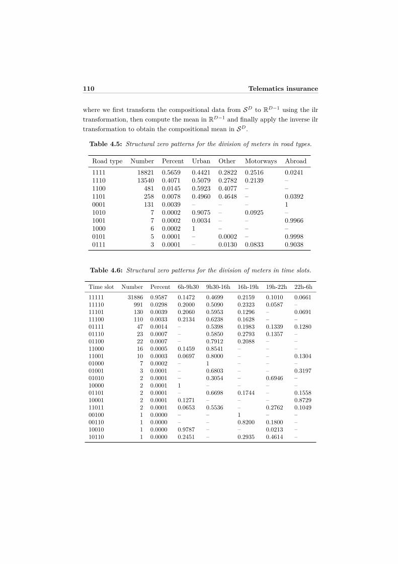
110 Telematics insurance
where we first transform the compositional data from SD to RD−1 using the ilrtransformation, then compute the mean in RD−1 and finally apply the inverse ilrtransformation to obtain the compositional mean in SD.
Table 4.5: Structural zero patterns for the division of meters in road types.
Road type Number Percent Urban Other Motorways Abroad1111 18821 0.5659 0.4421 0.2822 0.2516 0.02411110 13540 0.4071 0.5079 0.2782 0.2139 –1100 481 0.0145 0.5923 0.4077 – –1101 258 0.0078 0.4960 0.4648 – 0.03920001 131 0.0039 – – – 11010 7 0.0002 0.9075 – 0.0925 –1001 7 0.0002 0.0034 – – 0.99661000 6 0.0002 1 – – –0101 5 0.0001 – 0.0002 – 0.99980111 3 0.0001 – 0.0130 0.0833 0.9038
Table 4.6: Structural zero patterns for the division of meters in time slots.
Time slot Number Percent 6h-9h30 9h30-16h 16h-19h 19h-22h 22h-6h11111 31886 0.9587 0.1472 0.4699 0.2159 0.1010 0.066111110 991 0.0298 0.2000 0.5090 0.2323 0.0587 –11101 130 0.0039 0.2060 0.5953 0.1296 – 0.069111100 110 0.0033 0.2134 0.6238 0.1628 – –01111 47 0.0014 – 0.5398 0.1983 0.1339 0.128001110 23 0.0007 – 0.5850 0.2793 0.1357 –01100 22 0.0007 – 0.7912 0.2088 – –11000 16 0.0005 0.1459 0.8541 – – –11001 10 0.0003 0.0697 0.8000 – – 0.130401000 7 0.0002 – 1 – – –01001 3 0.0001 – 0.6803 – – 0.319701010 2 0.0001 – 0.3054 – 0.6946 –10000 2 0.0001 1 – – – –01101 2 0.0001 – 0.6698 0.1744 – 0.155810001 2 0.0001 0.1271 – – – 0.872911011 2 0.0001 0.0653 0.5536 – 0.2762 0.104900100 1 0.0000 – – 1 – –00110 1 0.0000 – – 0.8200 0.1800 –10010 1 0.0000 0.9787 – – 0.0213 –10110 1 0.0000 0.2451 – 0.2935 0.4614 –
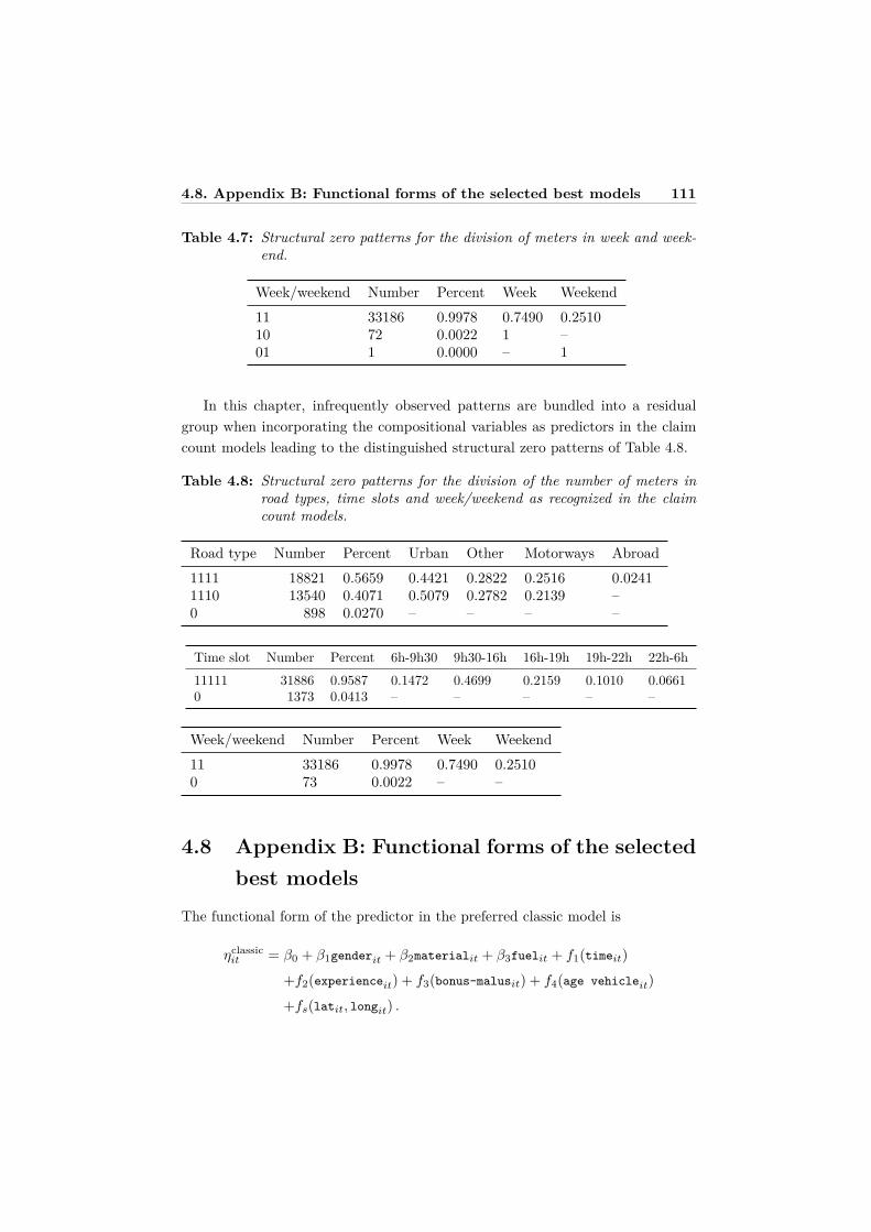
4.8. Appendix B: Functional forms of the selected best models 111
Table 4.7: Structural zero patterns for the division of meters in week and week-end.
Week/weekend Number Percent Week Weekend11 33186 0.9978 0.7490 0.251010 72 0.0022 1 –01 1 0.0000 – 1
In this chapter, infrequently observed patterns are bundled into a residualgroup when incorporating the compositional variables as predictors in the claimcount models leading to the distinguished structural zero patterns of Table 4.8.
Table 4.8: Structural zero patterns for the division of the number of meters inroad types, time slots and week/weekend as recognized in the claimcount models.
Road type Number Percent Urban Other Motorways Abroad1111 18821 0.5659 0.4421 0.2822 0.2516 0.02411110 13540 0.4071 0.5079 0.2782 0.2139 –0 898 0.0270 – – – –
Time slot Number Percent 6h-9h30 9h30-16h 16h-19h 19h-22h 22h-6h11111 31886 0.9587 0.1472 0.4699 0.2159 0.1010 0.06610 1373 0.0413 – – – – –
Week/weekend Number Percent Week Weekend11 33186 0.9978 0.7490 0.25100 73 0.0022 – –
4.8 Appendix B: Functional forms of the selectedbest models
The functional form of the predictor in the preferred classic model is
ηclassicit = β0 + β1genderit + β2materialit + β3fuelit + f1(timeit)
+f2(experienceit) + f3(bonus-malusit) + f4(age vehicleit)
+fs(latit, longit) .

112 Telematics insurance
The predictor in the best time-hybrid model can be written as
ηtime-hybridit = β0 + β1materialit + β2fuelit + f1(time)it + f2(experienceit)
+f3(bonus-malusit) + f4(age vehicleit) + fs(latit, longit)
+f5(yearly distanceit) + f6(average distanceit)
+droad(1111)〈b
road(1111),x(1111)〉a + droad
(1110)〈broad(1110),x(1110)〉a
+(1− droad(1111) − droad
(1110))broad0 + dtime
(11111)〈btime(11111),x(11111)〉a
+(1− dtime(11111))btime
0 + dweek(11) 〈b
week(11) ,x(11)〉a + (1− dweek
(11) )bweek0 ,
and for the preferred meter-hybrid model we have
ηmeter-hybridit = β0 + β1materialit + β2fuelit + f1(experienceit)
+f2(bonus-malusit) + f3(age vehicleit) + fs(latit, longit)
+f4(distanceit) + f5(average distanceit)
+droad(1111)〈b
road(1111),x(1111)〉a + droad
(1110)〈broad(1110),x(1110)〉a
+(1− droad(1111) − droad
(1110))broad0 + dtime
(11111)〈btime(11111),x(11111)〉a
+(1− dtime(11111))btime
0 + dweek(11) 〈b
week(11) ,x(11)〉a + (1− dweek
(11) )bweek0 .
Finally, the predictor in the best telematics model is given by
ηtelematicsit = β0 + f1(distance)it + f2(average distanceit)
+droad(1111)〈b
road(1111),x(1111)〉a + droad
(1110)〈broad(1110),x(1110)〉a
+(1− droad(1111) − droad
(1110))broad0 + dtime
(11111)〈btime(11111),x(11111)〉a
+(1− dtime(11111))btime
0 + dweek(11) 〈b
week(11) ,x(11)〉a + (1− dweek
(11) )bweek0 .
4.9 Appendix C: Graphical model displays
The effects of each predictor variable in the best classic model (resp. telematicsmodel) without offset restriction are graphically displayed in Figure 4.7 (resp Fig-ure 4.8). Similarly, the effects of each predictor variable in the best meter-hybridmodel without offset restriction are graphically displayed in Figure 4.9 for thepolicy model terms and Figure 4.10 for the telematics model terms.
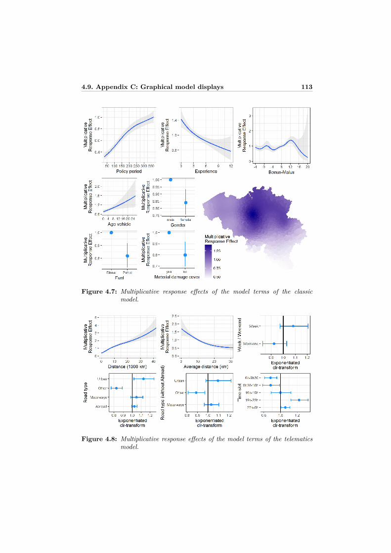
4.9. Appendix C: Graphical model displays 113
Figure 4.7: Multiplicative response effects of the model terms of the classicmodel.
Figure 4.8: Multiplicative response effects of the model terms of the telematicsmodel.
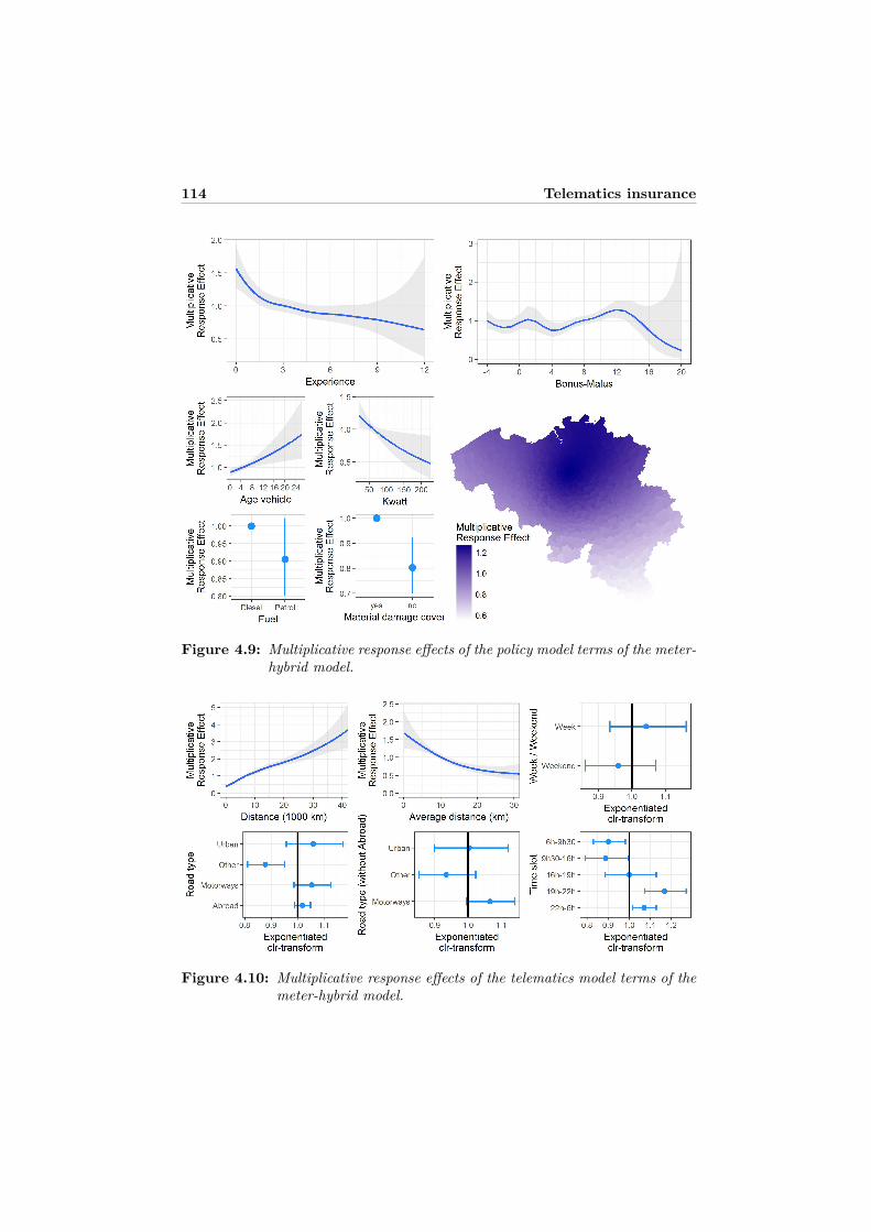
114 Telematics insurance
Figure 4.9: Multiplicative response effects of the policy model terms of the meter-hybrid model.
Figure 4.10: Multiplicative response effects of the telematics model terms of themeter-hybrid model.
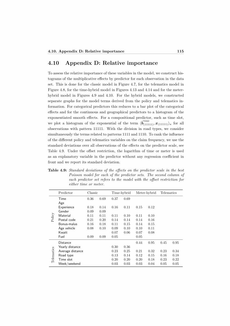
4.10. Appendix D: Relative importance 115
4.10 Appendix D: Relative importance
To assess the relative importance of these variables in the model, we construct his-tograms of the multiplicative effects by predictor for each observation in the dataset. This is done for the classic model in Figure 4.7, for the telematics model inFigure 4.8, for the time-hybrid model in Figures 4.13 and 4.14 and for the meter-hybrid model in Figures 4.9 and 4.10. For the hybrid models, we constructedseparate graphs for the model terms derived from the policy and telematics in-formation. For categorical predictors this reduces to a bar plot of the categoricaleffects and for the continuous and geographical predictors to a histogram of theexponentiated smooth effects. For a compositional predictor, such as time slot,we plot a histogram of the exponential of the term 〈b
time(11111),x(11111)〉a for all
observations with pattern 11111. With the division in road types, we considersimultaneously the terms related to patterns 1111 and 1110. To rank the influenceof the different policy and telematics variables on the claim frequency, we use thestandard deviations over all observations of the effects on the predictor scale, seeTable 4.9. Under the offset restriction, the logarithm of time or meter is usedas an explanatory variable in the predictor without any regression coefficient infront and we report its standard deviation.
Table 4.9: Standard deviations of the effects on the predictor scale in the bestPoisson model for each of the predictor sets. The second column ofeach predictor set refers to the model with the offset restriction foreither time or meter.
Predictor Classic Time-hybrid Meter-hybrid Telematics
Polic
y
Time 0.36 0.69 0.37 0.69AgeExperience 0.18 0.14 0.16 0.11 0.15 0.12Gender 0.09 0.09Material 0.11 0.11 0.11 0.10 0.11 0.10Postal code 0.21 0.20 0.14 0.14 0.14 0.16Bonus-malus 0.16 0.18 0.11 0.15 0.14 0.15Age vehicle 0.08 0.10 0.09 0.10 0.10 0.11Kwatt 0.07 0.06 0.07 0.08Fuel 0.09 0.09 0.05 0.05
Tele
mat
ics
Distance 0.44 0.95 0.45 0.95Yearly distance 0.30 0.36Average distance 0.23 0.25 0.21 0.32 0.23 0.34Road type 0.13 0.14 0.12 0.15 0.16 0.18Time slot 0.20 0.20 0.20 0.18 0.23 0.22Week/weekend 0.03 0.03 0.03 0.04 0.05 0.05
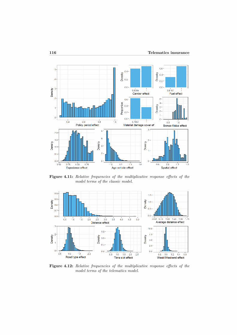
116 Telematics insurance
Figure 4.11: Relative frequencies of the multiplicative response effects of themodel terms of the classic model.
Figure 4.12: Relative frequencies of the multiplicative response effects of themodel terms of the telematics model.
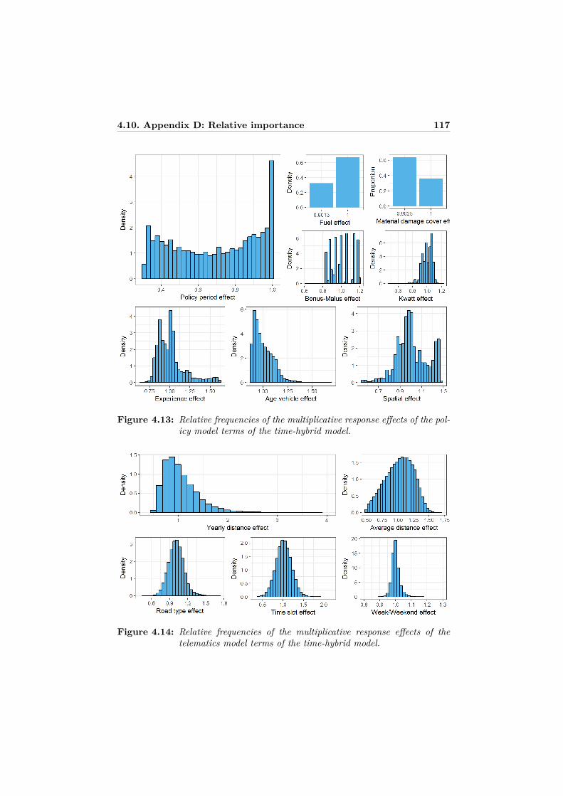
4.10. Appendix D: Relative importance 117
Figure 4.13: Relative frequencies of the multiplicative response effects of the pol-icy model terms of the time-hybrid model.
Figure 4.14: Relative frequencies of the multiplicative response effects of thetelematics model terms of the time-hybrid model.
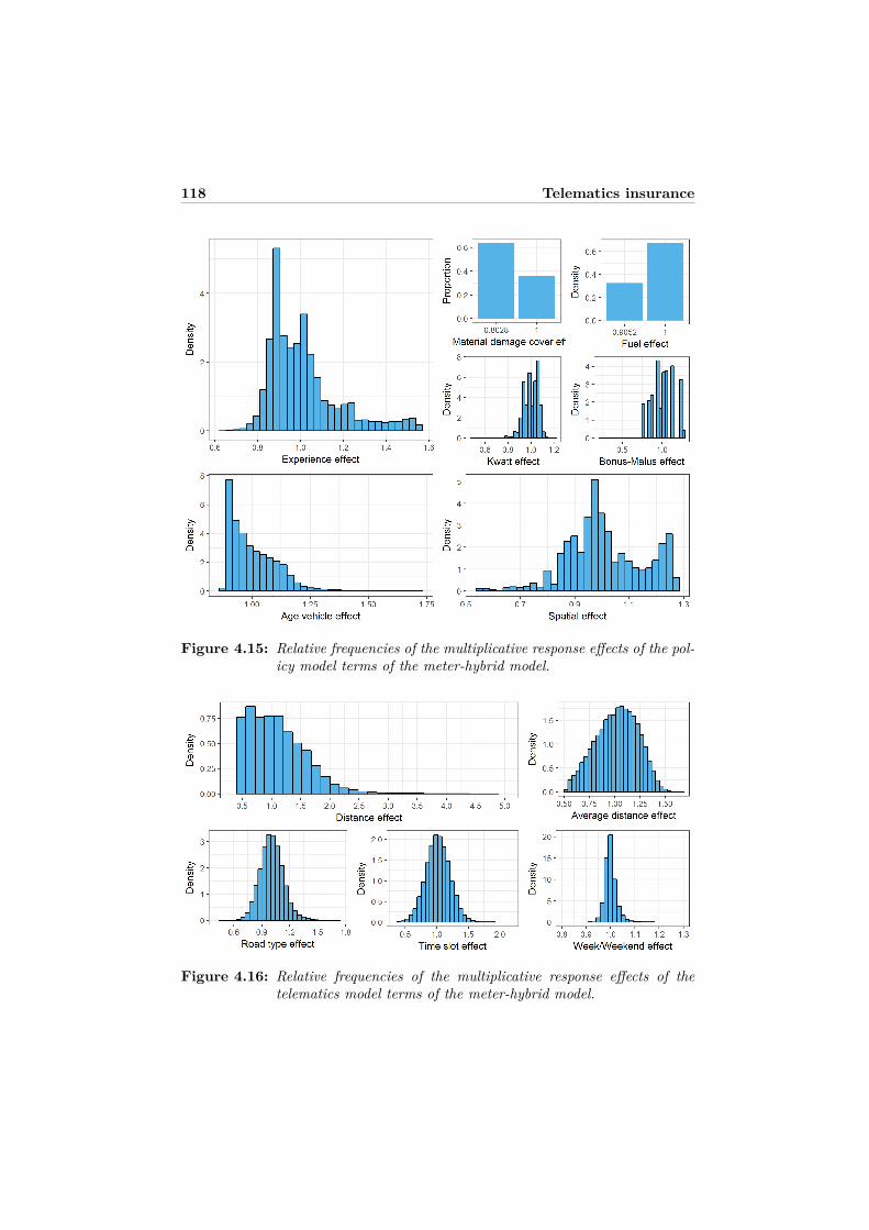
118 Telematics insurance
Figure 4.15: Relative frequencies of the multiplicative response effects of the pol-icy model terms of the meter-hybrid model.
Figure 4.16: Relative frequencies of the multiplicative response effects of thetelematics model terms of the meter-hybrid model.

Chapter 5
Predicting daily IBNR claim
counts using a regression
approach for the occurrence of
claims and their reporting delay
Abstract
Insurance companies need to hold capital to be able to fulfill future liabili-ties with respect to the policies they write. Due to the delay in the reportingof claims, not all of the claims that occurred in the past have been observedyet. The accurate estimation of the number of incurred but not reportedclaims forms an essential part of claims reserving. We present a flexibleframework to model and jointly estimate the occurrence and reporting ofclaims. A regression approach is used to capture the seasonal effects of themonth, day of the week and day of the month of the occurrence date and toincorporate the proportional effect of exposure on claim occurrences. Pa-rameter estimates are obtained using the EM algorithm by regarding thedaily run-off triangle of claims as an incomplete data problem. The re-sulting method is elegant, easy to understand and implement, and providesrefined forecasts on a daily level. The proposed methodology is applied toa European general liability portfolio. Initial insight into the data set moti-vates us to model the reporting delays in weeks combined with day-specificreporting probabilities. The performance of our model is evaluated basedon out-of-sample data.
119
120 IBNR claims reserving
This chapter is based on Verbelen, R., Antonio, K., Claeskens, G. and Crevecoeur,J. (2017). Predicting daily IBNR claim counts using a regression approach forthe occurrence of claims and their reporting delay. Working paper.
5.1 Introduction
Insurance companies need to hold sufficient reserves in order to be able to fulfillfuture liabilities with respect to outstanding claims. These reserves are a key fac-tor on the liability side of the balance sheet of the insurance company. Accurate,reliable and stable reserving methods for a wide range of products and lines ofbusiness are crucial to safeguard solvency, stability and profitability. With theintroduction of new regulatory guidelines for the European insurance business inthe form of Solvency II, the insurance industry has regained interest in using moreelaborate methodology to model future cash flows and meet regulators’ increas-ing requirements. Insurance companies are strongly encouraged to supplement adhoc, deterministic methods with fully stochastic approaches, aiming at accuratelyreflecting the riskiness in the portfolio under consideration.
The development of a single claim is visualized in the time line of Figure 5.1.A claim occurs at a certain occurrence date socc, consequently it is declared tothe insurer at reporting date srep and one or several payments follow (at timess1 , s2 and s3) until the closure of the claim at settlement date sset. Claims arenot reported instantaneously to the insurer, but always after a certain reportingdelay. This delay reflects the time gap between the occurrence of the claim andthe reporting to the insurance company, which can for instance be due to the factthat the policyholder did not immediately notify his agent or only noticed theclaim after a while. After notification, claims are also not settled immediatelybecause it usually takes time to evaluate the whole size of the claim. Expertshave to ascertain the loss or damage and the insured and the insurance companymust come to an agreement. The settlement delay is sometimes further extendeddue to additional investigations or disputes which have to be settled in court.Intermediate payments of justified claim benefits are paid along the way whichcan lead to a sequence of multiple cash flows before final settlement.
When an insurance company closes its books, it needs to predict future cashflows of claims that have occurred in the past and are only settled in the futurein order to set aside adequate premium reserves (see e.g. Wuthrich and Merz,2008). This assessment of the outstanding loss liabilities of past claims is referred
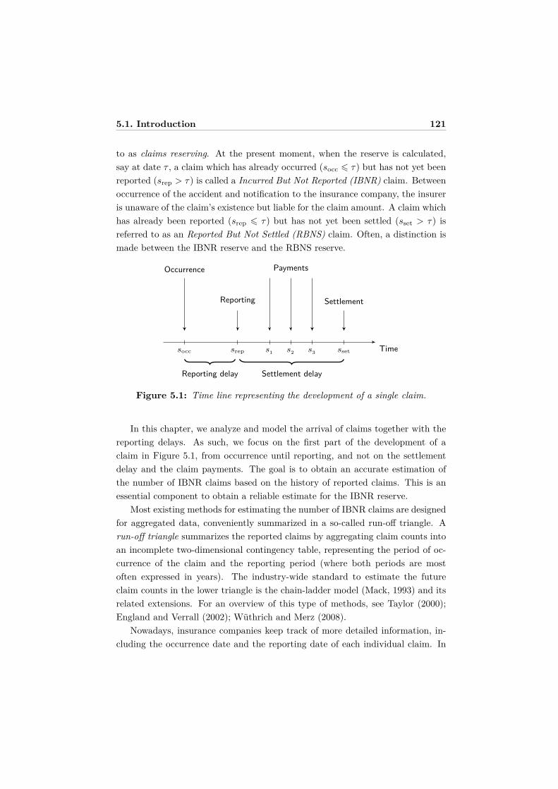
5.1. Introduction 121
to as claims reserving. At the present moment, when the reserve is calculated,say at date τ , a claim which has already occurred (socc 6 τ) but has not yet beenreported (srep > τ) is called a Incurred But Not Reported (IBNR) claim. Betweenoccurrence of the accident and notification to the insurance company, the insureris unaware of the claim’s existence but liable for the claim amount. A claim whichhas already been reported (srep 6 τ) but has not yet been settled (sset > τ) isreferred to as an Reported But Not Settled (RBNS) claim. Often, a distinction ismade between the IBNR reserve and the RBNS reserve.
Timesocc srep s1 s2 s3 sset
Occurrence
Reporting
Payments
Settlement
Reporting delay Settlement delay
Figure 5.1: Time line representing the development of a single claim.
In this chapter, we analyze and model the arrival of claims together with thereporting delays. As such, we focus on the first part of the development of aclaim in Figure 5.1, from occurrence until reporting, and not on the settlementdelay and the claim payments. The goal is to obtain an accurate estimation ofthe number of IBNR claims based on the history of reported claims. This is anessential component to obtain a reliable estimate for the IBNR reserve.
Most existing methods for estimating the number of IBNR claims are designedfor aggregated data, conveniently summarized in a so-called run-off triangle. Arun-off triangle summarizes the reported claims by aggregating claim counts intoan incomplete two-dimensional contingency table, representing the period of oc-currence of the claim and the reporting period (where both periods are mostoften expressed in years). The industry-wide standard to estimate the futureclaim counts in the lower triangle is the chain-ladder model (Mack, 1993) and itsrelated extensions. For an overview of this type of methods, see Taylor (2000);England and Verrall (2002); Wuthrich and Merz (2008).
Nowadays, insurance companies keep track of more detailed information, in-cluding the occurrence date and the reporting date of each individual claim. In
122 IBNR claims reserving
the so-called macro-level reserving techniques, such as the chain-ladder method,the available data is not fully used. Over the recent years, there has been increas-ing interest in micro-level reserving techniques, which make use of the insurancedata on a more granular level. We briefly discuss a number of recent contributionsfrom the actuarial science literature which use a micro-level approach to predictthe number of IBNR claims.
Martınez Miranda et al. (2013) extend the traditional chain-ladder frameworkfor the claim count data to a continuous chain-ladder setting. They reformulatethe classical actuarial technique of chain-ladder as a histogram type of estima-tor and replacing this histogram by a two-dimensional kernel density estimatorwith support on the triangle. By assuming a multiplicative kernel, the local lin-ear density estimate can be extrapolated to the whole square which provides aforecast for the IBNR claims in the lower triangle. The model can be applied todata recorded in continuous time, although it is illustrated in the paper on dataaggregated on a monthly level.
Verrall and Wuthrich (2016) construct an inhomogeneous marked Poisson pro-cess to explicitly model the claims arrival process and reporting delay in contin-uous time based on individual claims data. The intensity of the Poisson processincorporates a weekly period piece-wise constant pattern and a monthly seasonalparameter. A spliced distribution with three layers (small, middle and large) isused for the reporting delay. Due to the delay in the reporting of claims, themarked Poisson process is thinned which complicates direct maximum likelihoodestimation.
Badescu et al. (2016b,a) and Avanzi et al. (2016) propose to model the claimarrival process along with its reporting delays as a marked Cox process to allowfor overdispersion and serial dependency. A Cox process, or doubly stochasticPoisson process, extends a Poisson process by modeling the intensity as a non-negative stochastic process.
Badescu et al. (2016b) use a weekly piecewise constant stochastic processgenerated by a hidden Markov model (HMM) with state-dependent Erlang distri-butions. The discrete process of the number of observed claims during each weekthen follows a Pascal-HMM with scale parameters depending on the exposure andthe reporting delay distribution. Instead of joint estimation of all parameters, atwo-stage method is applied. In a first stage, the reporting delay distribution isestimated using a mixture of Erlangs. Observable reporting delays are howeverright-truncated at different thresholds, which the fitting algorithm of Verbelenet al. (2015) is not able to handle. This is dealt with by extracting information
5.1. Introduction 123
from the whole data set instead of only the training part, which is not possiblein practice. In a second stage, the parameters of the Pascal-HMM are estimatedusing an Expectation-Maximization (EM) algorithm by plugging in time-varyingscale parameters based on the fitted reporting delay distribution.
Avanzi et al. (2016) use a continuous time shot noise process to model theclaim occurrence process, allowing for varying exposure and reporting delays. Forparameter estimation, claim counts are no longer regarded in continuous time butdiscretized by week and, when calculating the reporting delay probabilities, it isassumed that the arrival time is the middle of the week. Joint estimation of allparameters relies on a complex Monte Carlo Expectation-Maximization (MCEM)algorithm with a Reversible Jump Markov Chain Monte Carlo (RJMCMC) filtersince the likelihood of the Cox process unconditional on the shot noise processinvolves a high dimensional integral, which is not computationally efficient tocalculate.
Beyond the field of actuarial science, similar statistical problems are also en-countered in the research fields of biostatistics and epidemiology (see e.g. Harris,1990; Lawless, 1994; Pagano et al., 1994; Midthune et al., 2005). For instance,when estimating the incidence of a disease, it is necessary to account for delaysin the reporting of cases. Moreover, statistical surveillance systems for the timelydetection of outbreaks of infectious disease have to properly adjust for these re-porting delays in order to take timely preventive action (see e.g. Noufaily et al.,2015, 2016).
In our work, we present a new technique to estimate the number of eventssubject to a reporting delay by explicitly modeling both the occurrence processof the events and the reporting delay distribution using flexible regression ap-proaches. We specifically focus on the case of IBNR claims in insurance, but ourwork can also be applied in the fields mentioned earlier. In practice, insurancecompanies register the occurrence date and the corresponding reporting date foreach observed claim in their administrative systems, rather than the exact occur-rence times or reporting times. We recognize this natural time unit of one dayby constructing our models on this level instead of considering continuous timemodels (such as the Poisson or Cox processes) or aggregated versions by week,month or year (such as the traditional chain-ladder method).
A regression approach allows us to incorporate seasonal effects in both theoccurrences of claims and the reporting delays. These effects can be caused byvarious time factors, such as the day of week, the day of month, or the month ofthe occurrence date, as well as relevant external information (if available), such
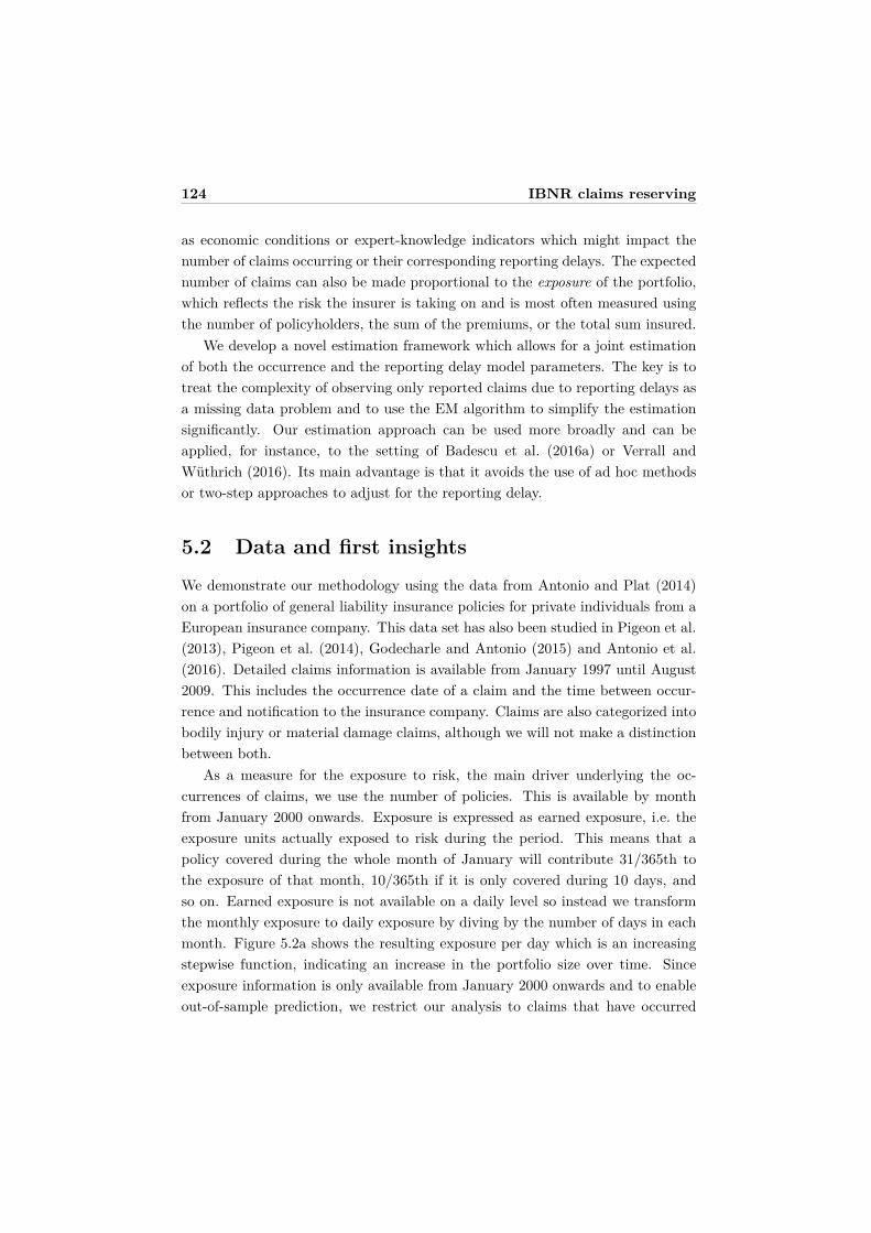
124 IBNR claims reserving
as economic conditions or expert-knowledge indicators which might impact thenumber of claims occurring or their corresponding reporting delays. The expectednumber of claims can also be made proportional to the exposure of the portfolio,which reflects the risk the insurer is taking on and is most often measured usingthe number of policyholders, the sum of the premiums, or the total sum insured.
We develop a novel estimation framework which allows for a joint estimationof both the occurrence and the reporting delay model parameters. The key is totreat the complexity of observing only reported claims due to reporting delays asa missing data problem and to use the EM algorithm to simplify the estimationsignificantly. Our estimation approach can be used more broadly and can beapplied, for instance, to the setting of Badescu et al. (2016a) or Verrall andWuthrich (2016). Its main advantage is that it avoids the use of ad hoc methodsor two-step approaches to adjust for the reporting delay.
5.2 Data and first insights
We demonstrate our methodology using the data from Antonio and Plat (2014)on a portfolio of general liability insurance policies for private individuals from aEuropean insurance company. This data set has also been studied in Pigeon et al.(2013), Pigeon et al. (2014), Godecharle and Antonio (2015) and Antonio et al.(2016). Detailed claims information is available from January 1997 until August2009. This includes the occurrence date of a claim and the time between occur-rence and notification to the insurance company. Claims are also categorized intobodily injury or material damage claims, although we will not make a distinctionbetween both.
As a measure for the exposure to risk, the main driver underlying the oc-currences of claims, we use the number of policies. This is available by monthfrom January 2000 onwards. Exposure is expressed as earned exposure, i.e. theexposure units actually exposed to risk during the period. This means that apolicy covered during the whole month of January will contribute 31/365th tothe exposure of that month, 10/365th if it is only covered during 10 days, andso on. Earned exposure is not available on a daily level so instead we transformthe monthly exposure to daily exposure by diving by the number of days in eachmonth. Figure 5.2a shows the resulting exposure per day which is an increasingstepwise function, indicating an increase in the portfolio size over time. Sinceexposure information is only available from January 2000 onwards and to enableout-of-sample prediction, we restrict our analysis to claims that have occurred
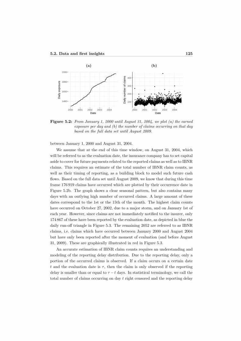
5.2. Data and first insights 125
(a)
1400
1600
1800
2000
2000 2001 2002 2003 2004
Date
Dai
ly e
xpos
ure
(b)
●
●●
●
●
●●
●●●
●●●●
●
●
●●
●●●
●
●●
●
●●
●●
●
●
●
●●●
●
●
●●
●
●
●
●
●
●●●
●
●
●●
●
●●
●
●
●●
●
●
●
●
●●
●
●●
●●●
●
●
●
●
●
●●
●●
●
●
●
●●
●
●●●●●
●
●
●
●●●●
●●●●
●●●
●
●
●
●
●
●
●
●●
●
●
●
●
●
●
●●
●
●●
●
●
●
●
●●
●
●
●
●
●
●
●
●
●
●
●
●
●●
●
●
●
●
●
●
●
●
●
●
●
●●●●
●●
●
●●
●
●
●
●●
●●
●
●
●●
●●●
●
●
●●
●
●
●
●●
●
●●
●
●
●
●●
●
●
●
●
●
●
●
●●●●●
●
●
●
●●
●
●
●●
●
●
●
●●●
●
●
●
●
●
●
●●
●●
●●
●●●●
●
●●
●
●
●
●●
●
●
●
●●
●
●
●●●
●
●
●
●
●
●●
●
●
●
●
●
●
●●●●
●●
●●●●●
●
●●
●●●●
●
●
●●●
●
●●
●●●●●●●
●
●
●
●
●
●●
●
●
●●●
●
●
●
●
●
●●
●●
●
●
●●●
●
●
●
●
●●
●
●●
●
●
●
●
●●
●
●●
●●
●
●
●
●●●
●
●●
●
●
●
●
●●●
●
●
●
●●
●
●
●
●
●
●●
●
●●
●
●
●●
●●●●
●
●●●
●
●
●
●
●●
●●●
●●
●●
●●
●
●●●
●●
●
●
●●●●●
●
●
●
●
●
●
●
●
●
●●
●
●●
●
●
●●
●
●
●
●
●
●
●●●
●●
●
●●
●●●
●●
●
●
●
●
●
●
●
●
●
●
●●●
●
●
●●
●●
●●
●
●●
●
●●
●●
●
●
●
●
●
●
●
●
●
●
●●●●
●
●
●●
●
●●
●●
●
●
●
●
●●●
●
●
●
●
●●
●
●
●●
●
●●●●
●
●●
●
●
●
●
●●
●●●
●
●●
●
●
●
●●
●
●
●
●
●●●
●
●●●
●
●●●
●
●●●●●●
●
●
●
●
●
●
●
●
●●●●
●
●●
●●
●●
●
●
●●
●
●
●
●
●
●
●
●
●●
●●●
●
●
●●
●●●
●
●
●●
●●
●
●
●
●
●●●●
●
●
●●
●
●●
●●●
●
●●●
●●
●●
●
●
●●
●
●
●
●
●
●
●
●
●●
●
●
●●●
●
●●●
●
●●
●
●
●●
●●
●
●●
●
●●●●
●
●●●●
●●●●
●
●●●
●
●
●●
●
●
●
●
●
●
●
●●●
●
●●
●
●●●
●
●
●
●
●
●
●
●
●
●
●
●
●
●
●
●
●
●●
●
●
●
●●
●
●
●●
●
●●
●
●
●
●
●
●
●
●●●
●●
●
●●
●●
●
●●●
●
●
●
●●
●
●●
●
●
●
●
●●
●
●●
●
●●
●
●
●●
●
●
●
●
●●
●
●
●
●●
●
●
●
●
●
●
●●●●●
●
●
●
●●●
●
●
●
●●
●
●
●●
●●
●●
●
●
●
●●
●●
●
●●
●
●●
●
●●
●●●●
●
●●
●
●●
●
●
●
●●
●
●
●
●●●
●
●
●
●
●
●●
●
●
●
●●●
●
●
●
●●●
●
●
●
●
●
●●●●
●
●
●
●
●
●
●●
●●
●●●●
●●
●
●
●
●●
●
●
●
●
●●●
●
●
●
●
●●
●
●●●●●
●
●●●
●
●
●●●
●
●
●
●
●
●
●
●
●●●
●●
●
●
●
●
●
●
●
●●
●
●
●●●
●
●
●●●
●●
●●
●
●●
●
●
●●
●
●
●
●
●
●
●
●●
●
●
●●
●
●●
●●●
●
●
●
●
●
●●
●
●●
●
●
●
●●
●
●
●
●
●●
●
●
●
●
●●●●
●
●
●
●●
●
●●
●●
●
●●●
●
●
●
●●●●
●
●
●●
●●●
●
●●
●
●●
●●
●
●●●●
●
●●
●
●
●●
●
●
●
●
●
●
●●
●
●●●●●
●
●
●
●●
●
●●
●
●
●
●●
●
●●
●
●
●
●
●●
●
●●●
●
●
●
●●●
●
●
●
●
●
●●●
●
●
●
●
●
●●●●
●
●
●●
●
●
●●
●
●
●
●
●
●
●
●
●
●●
●●●
●●●
●●●
●●
●
●
●
●●
●
●
●●
●
●●●
●●●
●
●●
●
●
●
●
●
●
●●●
●
●●●
●
●
●●●
●
●
●
●
●
●
●
●●
●
●
●
●
●●●●●●●
●
●
●
●
●
●
●
●
●
●●●●●
●●●
●●
●
●
●
●●●
●
●
●●
●
●●
●
●●
●
●
●●●
●
●
●
●●
●
●
●
●●
●
●
●
●
●●
●
●
●●●
●
●
●
●
●●
●
●●●
●
●
●
●
●●●
●
●●
●
●●
●●
●
●
●●●●
●●●
●
●
●
●
●●●●
●●●
●●●●
●●
●
●
●●
●
●
●
●
●
●●●
●
●●●
●
●
●
●
●●●
●
●
●●
●
●
●
●
●
●
●
●
●
●
●
●●
●
●
●●●
●
●
●
●
●
●
●
●
●●
●
●
●●●
●
●
●●●●●●●●●
●●
●
●
●
●
●
●
●
●
●
●
●●
●
●
●
●
●
●
●
●
●
●
●
●
●
●
●●
●
●
●
●
●●
●
●
●
●
●
●
●●●●
●
●●●●
●
●
●
●●
●
●●●
●
●●●
●●●
●
●
●
●
●
●
●
●
●
●
●●
●●
●
●
●●●●
●●●
●
●
●
●
●
●
●
●
●●
●
●●
●
●
●
●
●●
●
●
●●
●
●●
●
●
●
●
●
●●
●
●●●
●
●
●●
●●
●
●
●
●
●
●
●
●
●
●
●●
●
●
●
●
●
●●
●●●●
●
●
●
●●
●
●
●
●
●●
●
●●●
●
●
●
●●●
●●
●
●●●●
●
●
●
●●
●
●
●
●
●●
●
●
●●●
●
●●●●
●
●
●
●●
●
●
●
●
●
●●●
●
●
●
●
●●●●●
●
●
●
●
●●
●
●
●
●
●●●●
●
●
●
●●●
●
●
●
●
●
●
●●
●
●●●
●
●
●
●●
●
●
●●●
●
●
●
●●●●
●
●
●
●
●100
200
300
400
2000 2001 2002 2003 2004
Date
Dai
ly n
umbe
r of
cla
ims
Figure 5.2: From January 1, 2000 until August 31, 2004, we plot (a) the earnedexposure per day and (b) the number of claims occurring on that daybased on the full data set until August 2009.
between January 1, 2000 and August 31, 2004.We assume that at the end of this time window, on August 31, 2004, which
will be referred to as the evaluation date, the insurance company has to set capitalaside to cover for future payments related to the reported claims as well as to IBNRclaims. This requires an estimate of the total number of IBNR claim counts, aswell as their timing of reporting, as a building block to model such future cashflows. Based on the full data set until August 2009, we know that during this timeframe 176 919 claims have occurred which are plotted by their occurrence date inFigure 5.2b. The graph shows a clear seasonal pattern, but also contains manydays with an outlying high number of occurred claims. A large amount of thesedates correspond to the 1st or the 15th of the month. The highest claim countshave occurred on October 27, 2002, due to a major storm, and on January 1st ofeach year. However, since claims are not immediately notified to the insurer, only174 867 of these have been reported by the evaluation date, as depicted in blue thedaily run-off triangle in Figure 5.3. The remaining 2052 are referred to as IBNRclaims, i.e. claims which have occurred between January 2000 and August 2004but have only been reported after the moment of evaluation (and before August31, 2009). These are graphically illustrated in red in Figure 5.3.
An accurate estimation of IBNR claim counts requires an understanding andmodeling of the reporting delay distribution. Due to the reporting delay, only aportion of the occurred claims is observed. If a claim occurs on a certain datet and the evaluation date is τ , then the claim is only observed if the reportingdelay is smaller than or equal to τ − t days. In statistical terminology, we call thetotal number of claims occurring on day t right censored and the reporting delay
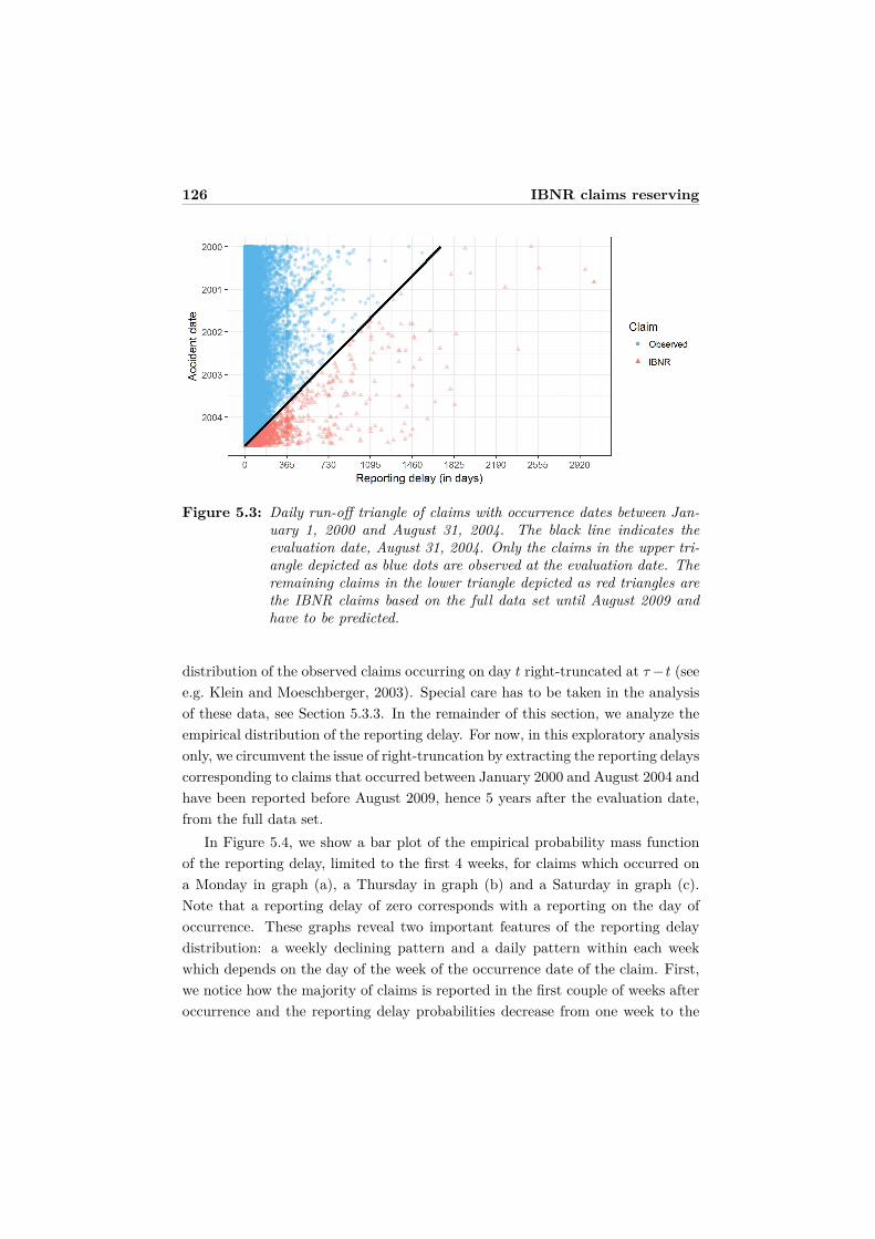
126 IBNR claims reserving
Figure 5.3: Daily run-off triangle of claims with occurrence dates between Jan-uary 1, 2000 and August 31, 2004. The black line indicates theevaluation date, August 31, 2004. Only the claims in the upper tri-angle depicted as blue dots are observed at the evaluation date. Theremaining claims in the lower triangle depicted as red triangles arethe IBNR claims based on the full data set until August 2009 andhave to be predicted.
distribution of the observed claims occurring on day t right-truncated at τ−t (seee.g. Klein and Moeschberger, 2003). Special care has to be taken in the analysisof these data, see Section 5.3.3. In the remainder of this section, we analyze theempirical distribution of the reporting delay. For now, in this exploratory analysisonly, we circumvent the issue of right-truncation by extracting the reporting delayscorresponding to claims that occurred between January 2000 and August 2004 andhave been reported before August 2009, hence 5 years after the evaluation date,from the full data set.
In Figure 5.4, we show a bar plot of the empirical probability mass functionof the reporting delay, limited to the first 4 weeks, for claims which occurred ona Monday in graph (a), a Thursday in graph (b) and a Saturday in graph (c).Note that a reporting delay of zero corresponds with a reporting on the day ofoccurrence. These graphs reveal two important features of the reporting delaydistribution: a weekly declining pattern and a daily pattern within each weekwhich depends on the day of the week of the occurrence date of the claim. First,we notice how the majority of claims is reported in the first couple of weeks afteroccurrence and the reporting delay probabilities decrease from one week to the
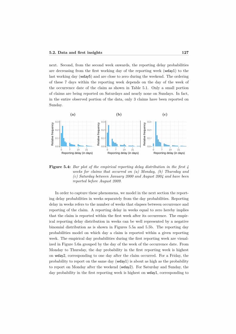
5.2. Data and first insights 127
next. Second, from the second week onwards, the reporting delay probabilitiesare decreasing from the first working day of the reporting week (wday1) to thelast working day (wday5) and are close to zero during the weekend. The orderingof these 7 days within the reporting week depends on the day of the week ofthe occurrence date of the claim as shown in Table 5.1. Only a small portionof claims are being reported on Saturdays and nearly none on Sundays. In fact,in the entire observed portion of the data, only 3 claims have been reported onSunday.
(a)
0.0
0.1
0.2
0.3
0 7 14 21
Reporting delay (in days)
Rel
ativ
e fr
eque
ncy
(b)
0.0
0.1
0.2
0.3
0 7 14 21
Reporting delay (in days)
Rel
ativ
e fr
eque
ncy
(c)
0.0
0.1
0.2
0.3
0 7 14 21
Reporting delay (in days)
Rel
ativ
e fr
eque
ncy
Figure 5.4: Bar plot of the empirical reporting delay distribution in the first 4weeks for claims that occurred on (a) Monday, (b) Thursday and(c) Saturday between January 2000 and August 2004 and have beenreported before August 2009.
In order to capture these phenomena, we model in the next section the report-ing delay probabilities in weeks separately from the day probabilities. Reportingdelay in weeks refers to the number of weeks that elapses between occurrence andreporting of the claim. A reporting delay in weeks equal to zero hereby impliesthat the claim is reported within the first week after its occurrence. The empir-ical reporting delay distribution in weeks can be well represented by a negativebinomial distribution as is shown in Figures 5.5a and 5.5b. The reporting dayprobabilities model on which day a claim is reported within a given reportingweek. The empirical day probabilities during the first reporting week are visual-ized in Figure 5.6a grouped by the day of the week of the occurrence date. FromMonday to Thursday, the day probability in the first reporting week is higheston wday2, corresponding to one day after the claim occurred. For a Friday, theprobability to report on the same day (wday1) is about as high as the probabilityto report on Monday after the weekend (wday2). For Saturday and Sunday, theday probability in the first reporting week is highest on wday1, corresponding to
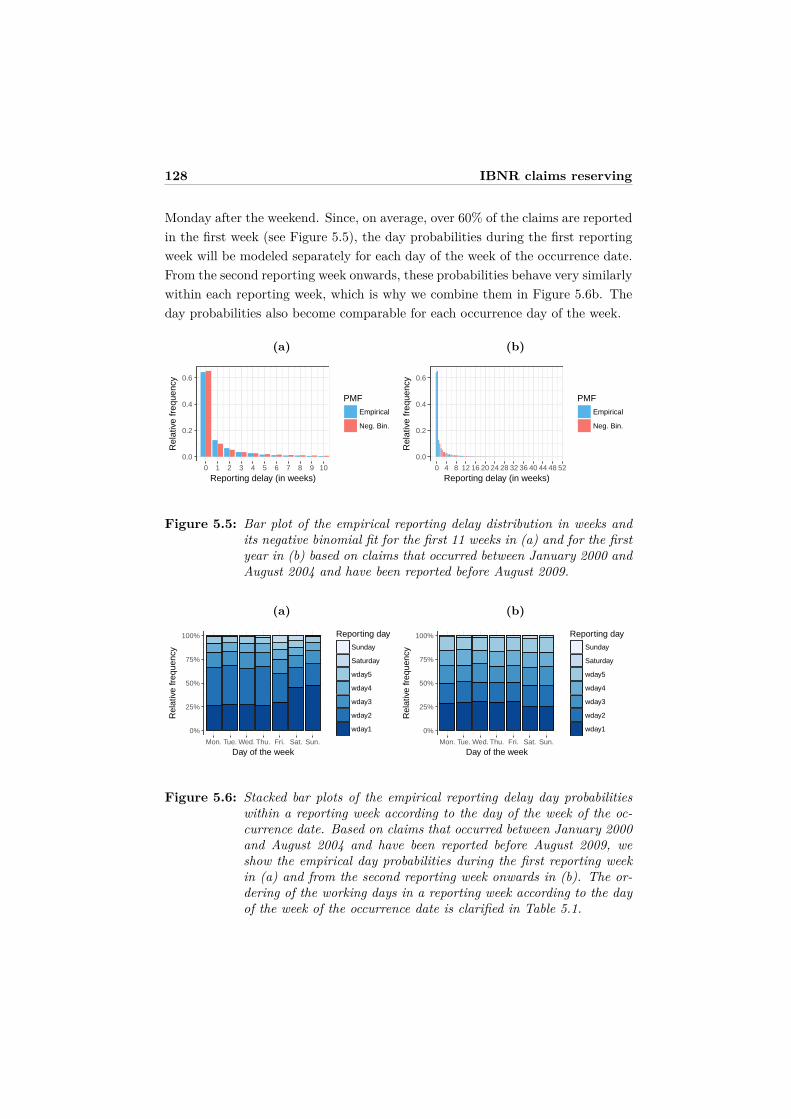
128 IBNR claims reserving
Monday after the weekend. Since, on average, over 60% of the claims are reportedin the first week (see Figure 5.5), the day probabilities during the first reportingweek will be modeled separately for each day of the week of the occurrence date.From the second reporting week onwards, these probabilities behave very similarlywithin each reporting week, which is why we combine them in Figure 5.6b. Theday probabilities also become comparable for each occurrence day of the week.
(a)
0.0
0.2
0.4
0.6
0 1 2 3 4 5 6 7 8 9 10
Reporting delay (in weeks)
Rel
ativ
e fr
eque
ncy
PMF
Empirical
Neg. Bin.
(b)
0.0
0.2
0.4
0.6
0 4 8 12 16 20 24 28 32 36 40 44 48 52
Reporting delay (in weeks)
Rel
ativ
e fr
eque
ncy
PMF
Empirical
Neg. Bin.
Figure 5.5: Bar plot of the empirical reporting delay distribution in weeks andits negative binomial fit for the first 11 weeks in (a) and for the firstyear in (b) based on claims that occurred between January 2000 andAugust 2004 and have been reported before August 2009.
(a)
0%
25%
50%
75%
100%
Mon. Tue. Wed. Thu. Fri. Sat. Sun.
Day of the week
Rel
ativ
e fr
eque
ncy
Reporting day
Sunday
Saturday
wday5
wday4
wday3
wday2
wday1
(b)
0%
25%
50%
75%
100%
Mon. Tue. Wed. Thu. Fri. Sat. Sun.
Day of the week
Rel
ativ
e fr
eque
ncy
Reporting day
Sunday
Saturday
wday5
wday4
wday3
wday2
wday1
Figure 5.6: Stacked bar plots of the empirical reporting delay day probabilitieswithin a reporting week according to the day of the week of the oc-currence date. Based on claims that occurred between January 2000and August 2004 and have been reported before August 2009, weshow the empirical day probabilities during the first reporting weekin (a) and from the second reporting week onwards in (b). The or-dering of the working days in a reporting week according to the dayof the week of the occurrence date is clarified in Table 5.1.

5.3. The statistical model 129
Table 5.1: Ordering of the working days in the week (wday) by the day of theweek (dow) of the occurrence date. wday3, for example, denotes thethird working day of the reporting week, which is Wednesday when theclaim occurred on Monday and a Monday when the claim occurred onThursday, and so on.
wdaydow wday1 wday2 wday3 wday4 wday5 Saturday SundayMonday Monday Tuesday Wednesday Thursday Friday Saturday SundayTuesday Tuesday Wednesday Thursday Friday Monday Saturday SundayWednesday Wednesday Thursday Friday Monday Tuesday Saturday SundayThursday Thursday Friday Monday Tuesday Wednesday Saturday SundayFriday Friday Monday Tuesday Wednesday Thursday Saturday SundaySaturday Monday Tuesday Wednesday Thursday Friday Saturday SundaySunday Monday Tuesday Wednesday Thursday Friday Saturday Sunday
5.3 The statistical model
5.3.1 Daily claim count data
We model insurance claim counts on a daily level and denote the total number ofclaims which occurred on day t by Nt, where the integer t indicates the occurrencedate and ranges from 1 to τ . The number of these claims which have been reportedto the insurer after d days are denoted as Ntd such that
Nt =∞∑
d=0Ntd .
Due to this reporting delay, only part of these claims have been reported to theinsurer before or at the moment of evaluation, τ . Namely only those claims whichhave a reporting delay smaller than or equal to τ − t. We denote the observednumber of claims which occurred on day t by
NRt =
τ−t∑d=0
Ntd .
Only the observed claims NR = {Ntd | 1 6 t 6 τ, d > 0, t + d 6 τ} can be usedon the moment of evaluation when the outstanding claims liabilities have to becalculated. These can be represented in a daily run-off triangle as shown in Table5.2. The occurrence date is indicated in the rows and the reporting delay in thecolumns. Claim counts on the diagonal for which t+d is constant are all reported

130 IBNR claims reserving
on the same calendar day t + d, with τ being the last calendar day observed. Theobjective is to predict the IBNR claim counts N IBNR = {Ntd | 1 6 t 6 τ, d >
0, t+d > τ} in the lower part of the daily claims triangle in Table 5.2. We denotethe total IBNR claim counts per day by
N IBNRt =
∞∑d=τ−t+1
Ntd ,
and the total IBNR claim count over all occurrence days by
N IBNR =τ∑
t=1N IBNR
t =τ∑
t=1
∞∑d=τ−t+1
Ntd .
Table 5.2: Run-off triangle with daily claim counts. Only the claim counts inthe upper triangle are observed, whereas the claim counts in the lowertriangle have to be predicted.
Occurrence Reporting delay (in days)day 0 · · · τ − t · · · τ − 11 N10 · · · N1,τ−t · · · N1,τ−1...t Nt0 · · · Nt,τ−t
... IBNRτ Nτ0
5.3.2 Model assumptions
The statistical analysis of the daily claim counts using our proposed model isbased on the following two assumptions:
(A1) The daily total claim counts Nt for t = 1, . . . , τ are independently Poissondistributed with intensity λt = et exp(x′
tα), where et is the exposure, xt isthe vector of covariate information corresponding to occurrence day t andα is a parameter vector.
(A2) Conditional on Nt, the claim counts Ntd for d = 0, 1, 2, . . ., are multinomiallydistributed with probabilities ptd. These reporting delay probabilities are
5.3. The statistical model 131
structured as a product of week probabilities and day probabilities:
ptd =
pWt0 · p1
td for d < 7
pWt⌊
d7
⌋ · p2td otherwise.
The reporting delay week probabilities,
pWtw = Γ(φ + w)
w!Γ(φ)φφµw
t
(φ + µt)φ+wfor w = 0, 1, 2, . . . , (5.1)
are modeled using the probability mass function of a negative binomial dis-tribution with expected value µt = exp(z′
tβ) and variance µt + µ2t /φ, where
φ is the dispersion parameter and zt is the covariate vector correspondingto occurrence day t. The reporting delay day probabilities in the first weekcan be written in a symbolical way as
p1td = P1(dow(t), wday(t, t + d)) , (5.2)
where dow(t) denotes the day of the week of occurrence date t and wday(t, t+d) denotes the working day of the week of the reporting date t + d, giventhat the corresponding occurrence date is t. P1 is a 7× 7-matrix which hasrows and columns as in Table 5.1 and contains the day probabilities relatedto the first week. Each element in P1 is between 0 and 1 and all row sumsequal 1. Similarly, the reporting delay day probabilities from the secondweek onwards are given by
p2td = P2(wday(t, t + d)) , (5.3)
where P2 is a 1× 7-matrix which has columns as in Table 5.1 and elementsbetween 0 and 1 that sum up to 1.
Allowing for covariates in the model for the occurrences of claims as well as themodel for reporting delays in weeks allows us to build flexible models. The ex-pected number of claim occurrences can be made proportional to the exposureor depend on several measures of exposure. Evolutions over time or seasonaltrends can be captured to improve forecast predictions. Fluctuations in bothclaim counts and their reporting delays by month, day of the month or day of theweek of the occurrence date can be explicitly modeled. Additionally, an insurercan also model relationships with external covariates which might influence the
132 IBNR claims reserving
arrival process of claims. Potential effects might be plausible for economic circum-stances, business cycles and weather conditions. On top of that, the day-specificparticularities in the reporting delay we noticed in Section 5.1 and displayed inFigure 5.6 are captured using designated day probabilities.
5.3.3 Parameter estimation using the EM algorithm
We bundle the parameters to be estimated in Θ = {α,β, φ, P1, P2}. Based onthe assumptions in Section 5.3.2, the daily claim counts Ntd are independentlyPoisson distributed with intensities λtptd for t = 1, . . . , τ and d = 0, 1, 2, . . .. Thiscan be seen by writing the joint probability of Ntd = ntd for d = 0, 1, 2, . . . as theproduct of the probability of their sum Nt being equal to nt =
∑∞d=0 ntd and the
conditional multinomial probability:
P(Nt0 = nt0, Nt1 = nt1, Nt2 = nt2, . . .)
= P(Nt = nt) · P(Nt0 = nt0, Nt1 = nt1, Nt2 = nt2, . . . | Nt = nt)
= exp(−λt)λntt
nt!· nt!∏∞
d=0 ntd!·
∞∏d=0
(ptd)ntd
=∞∏
d=0
exp(−λtptd)(λtptd)ntd
ntd! ,
which factorizes into Poisson probabilities. This property is sometimes referred toas the thinning property of Poisson random variables. In particular, the observedclaim count NR
t on day t is Poisson distributed with intensity λtpRt where pR
t =∑τ−td=0 ptd and the IBNR claim count N IBNR
t is Poisson distributed with intensityλtp
IBNRt where pIBNR
t = 1 − pRt . Conditional on NR
t , the observed daily claimcounts {Ntd | d = 0, 1, . . . , τ − t} are multinomially distributed with parametersNR
t and {ptd/pRt | d = 0, 1, . . . , τ − t}, since we have to account for the right-
truncation of the reporting delay.The likelihood of the observed upper run-off triangle for our chosen model
can then be written as the product of a Poisson likelihood and a multinomiallikelihood,
L(Θ;NR) =τ∏
t=1
exp(−λtpRt )(λtp
Rt
)NRt
NRt !
NRt !∏τ−t
d=0 Ntd!
τ−t∏d=0
(ptd
pRt
)Ntd
. (5.4)
Equivalently, the likelihood can also be constructed by treating the daily claim
5.3. The statistical model 133
counts as right censored, since the number of IBNR claims is unknown,
L(Θ;NR) =τ∏
t=1
∞∑n=NR
t
exp(−λt)λnt
n! · n!∏τ−td=0 Ntd! · (n−NR
t )!
·τ−t∏d=0
(ptd)Ntd ·(pIBNR
t
)n−NRt .
Indeed, this expression reduces to (5.4) by rewriting the sum over n using theTaylor expansion for the exponential function. The corresponding log-likelihoodequals
logL(Θ;NR) = −τ∑
t=1λtp
Rt +
τ∑t=1
NRt log(λt)
+τ∑
t=1
τ−t∑d=0
Ntd log(ptd)−τ∑
t=1
τ−t∑d=0
log(Ntd!) . (5.5)
Note that, due to the right truncation of the reporting delay (or, the right censor-ing of the claim counts), the log-likelihood (5.5) contains terms which depend onthe parameters of both the Poisson model for claim occurrences and the report-ing delay distribution. This complicates direct maximum likelihood estimation asit prevents separate optimization with respect to each of these parameter blocks.Optimization using a standard numerical method such as Newton-Raphson is stillfeasible, but we cannot rely on statistical software packages and we need to derivethe analytical expressions of the gradient and Hessian of the log-likelihood (5.5).To simplify computations, shortcuts have been used to estimate parameters in re-lated works, such as plug-in estimates for the weekly periodic occurrence patternin Verrall and Wuthrich (2016) or a two-stage method in which the reporting de-lay distribution is estimated first and then plugged in to estimate the parametersrelated to the occurrence process (Antonio and Plat, 2014; Badescu et al., 2016a).
Instead, we choose to treat the truncation as a missing data problem andemploy the EM algorithm (Dempster et al., 1977; McLachlan and Krishnan, 2008)to simplify maximum likelihood parameter estimation. Consider the completeversion of the data N = NR∪N IBNR = {Ntd | 1 6 t 6 τ, d > 0} which augmentsthe observed daily claim counts from the upper part of the run-off triangle in Table5.2 with the unknown values of the future claim counts in the lower triangle. Given
134 IBNR claims reserving
the complete data N , we can construct the complete log-likelihood function
logLc(Θ;N) = −τ∑
t=1λt +
τ∑t=1
Nt log(λt)
+τ∑
t=1
∞∑d=0
Ntd log(ptd)−τ∑
t=1
∞∑d=0
log(Ntd!) . (5.6)
which allows for a separate estimation of the parameters of the claim occurrencemodel (appearing in λt) and those of the reporting delay distribution (appearingin ptd). The observed data log-likelihood (5.5) can be maximized by iterativelymaximizing the complete data log-likelihood (5.6) using the EM algorithm. How-ever, as we do not fully observe the complete data, the complete log-likelihood isa random variable. Therefore, it is not possible to directly optimize (5.6). Yet,the EM algorithm exploits the simpler form of the complete log-likelihood by it-erating between an E-step or expectation step and M-step or maximization step.Applied to our setting, the IBNR claim counts in the lower triangle of Table 5.2are replaced by their expected values in the E-step and the log-likelihood of theaugmented data is maximized in the M-step. The M-step will still require numer-ical optimization, but the parameters with respect to the claim occurrence modelcan be estimated separately from the reporting delay parameters and standardsoftware routines can be utilized in the absence of truncation. We discuss thesesteps in more detail.
E-step In the kth iteration of the E-step, we take the conditional expectationof the complete log-likelihood (5.5) given the incomplete data NR and using thecurrent estimate Θ(k−1) of the parameter vector Θ:
Q(Θ; Θ(k−1)) = E(
logLc(Θ;N) |NR; Θ(k−1))
. (5.7)
This requires us to compute the expected values of the future claim counts
N(k)td = E
[Ntd |NR; Θ(k−1)
]=
Ntd if d 6 τ − t
λ(k−1)t p
(k−1)td otherwise,
(5.8)
for t = 1, . . . , τ and the total daily claim counts N(k)t =
∑τ−td=0 Ntd+
∑∞d=τ−t+1 N
(k)td .
The terms in (5.7) containing E(
log(Ntd!) |NR; Θ(k−1))
do not play a role inthe EM algorithm as they do not depend on the unknown parameter vector Θ.
5.3. The statistical model 135
M-step In the kth iteration of the M-step, we maximize the expected value(5.7) of the complete data log-likelihood obtained in the E-step with respect tothe parameter vector Θ. In order to optimize (5.7) with respect to α as definedin model assumption (A1), we have to maximize the terms related to the claimoccurrence model,
−τ∑
t=1λt +
τ∑t=1
N(k)t log(λt) = −
τ∑t=1
et exp(x′tα) +
τ∑t=1
N(k)t (log(et) +x′
tα) , (5.9)
which is a weighted Poisson log-likelihood with an offset term (related to theexposure). The parameter values optimizing (5.9) are denoted by α(k). Basedon model assumption (A2), updating the estimates for the parameters of thereporting delay distribution requires the maximization of
τ∑t=1
∞∑d=0
N(k)td log(ptd) =
τ∑t=1
( ∞∑d=0
N(k)td log
(pW
t⌊
d7
⌋)+6∑
d=0N
(k)td log(p1
td)
+6∑
d=0N
(k)td log(p1
td) +∞∑
d=7N
(k)td log(p2
td))
.
From a numerical point of view, we truncate the infinite sums over the reportingdelay d at d = τ − 1, which corresponds to completing the run-off triangle inTable 5.2 without further extending it. Numerical experiments have shown thatthis choice is sufficiently high in our setting as the subsequent terms are negligible.The new parameter estimates β(k) and φ(k) of the negative binomial distributionfor the reporting delay in weeks are found by optimizing the weighted negativebinomial log-likelihood,
τ∑t=1
∞∑d=0
N(k)td log
(pW
t⌊
d7
⌋) =τ∑
t=1
∞∑w=0
( 6∑d=0
N(k)t,7w+d
)log(pW
tw
), (5.10)
where pWtw is given in (5.1) with µt = exp(z′
tβ). Both for optimizing (5.9) and(5.10), standard software packages can be used. Optimizing (5.7) with respect tothe day probabilities (5.2) and (5.3) and under the restriction that the sums ofthe rows (the sums over the working days of the week) equal 1 leads to
(P1(u, v)
)(k) =
∑t=1,...,τdow(t)=u
∑d=0,...,6
wday(t,t+d)=v
N(k)td∑
t=1,...,τdow(t)=u
∑6d=0 N
(k)td
,u = Monday, . . . , Sundayv = wday1, . . . , Sunday

136 IBNR claims reserving
and
(P2(v)
)(k) =
∑τt=1∑
d=7,...,∞wday(t,t+d)=v
N(k)td∑τ
t=1∑∞
d=7 N(k)td
, v = wday1, . . . , Sunday .
Initial step The first E-step of the EM algorithm with k = 1 requires a startingvalue Θ(0) for the parameter set. Our strategy is to first apply the chain-laddermethod on the daily claim counts to obtain initial predictions N
(0)td of the future
claim counts in the lower triangle of Table 5.2. Then, we initialize Θ by applyingan initial M-step based on these initial claim count estimates. More specifically,we define the cumulative claim counts as
Ctd =d∑
j=0Ntj for t = 1, . . . , τ, and d = 0, . . . , τ − 1 ,
and estimate the development factors of the chain-ladder technique on a dailylevel as
fd =∑τ−d
t=1 Ctd∑τ−dt=1 Ct,d−1
for d = 1, . . . , τ − 1 .
The chain-ladder technique applies these development factors to the latest cumu-lative claim count in each row to produce forecasts of future cumulative claimcounts:
Ct,d = Ct,τ−tfτ−t+1 . . . fd for t = 2, . . . , τ, and d = τ − t + 1, . . . , τ − 1 .
We use these chain-ladder estimates for the daily cumulative claim counts toinitialize the expected incremental claim counts as
N(0)td =
Ntd if d 6 τ − t
Ct,τ−t+1 − Ct,τ−t if d = τ − t + 1
Ctd − Ct,d−1 otherwise,
for t = 1, . . . , τ and apply an M-step, as outlined above with k = 0, to find decentstarting values Θ(0).
Convergence The log-likelihood (5.5) increases with each EM iteration (McLach-lan and Krishnan, 2008). Given proper starting values, the sequence Θ(k) con-verges to the maximum likelihood estimate (MLE) of Θ corresponding to the

5.3. The statistical model 137
(incomplete data) log-likelihood logL(Θ;NR) in (5.5). The stopping criterionwe apply is based on the relative change in the log-likelihood. Namely, we iterateuntil the absolute value of
logL(Θ(k);NR)− logL(Θ(k−1);NR)0.1 + logL(Θ(k);NR)
becomes sufficiently small. The parameter vector estimate upon convergence isdenoted by
Θ = {α, β, φ, P1, P2} .
5.3.4 Asymptotic variance-covariance matrix
The estimator for Θ obtained from the EM algorithm has the same limit as theMLE, whenever the starting value is adequately chosen. Hence, the maximumlikelihood asymptotic theory in terms of consistency, asymptotic normality andasymptotic efficiency applies. In particular, if we denote the (incomplete data)score statistic as
S(Θ;NR) = ∂
∂Θ logL(Θ;NR) ,
and the (incomplete data) observed information matrix
I(Θ;NR) = − ∂2
∂Θ∂Θ′ logL(Θ;NR) ,
then the asymptotic variance-covariance matrix of the MLE Θ is equal to theinverse of the (incomplete data) expected (Fisher) information matrix I(Θ) givenby
I(Θ) = E[I(Θ;NR) | Θ
]. (5.11)
The asymptotic variance-covariance matrix can be approximated by I−1(Θ). It isalso common practice to estimate this matrix using the inverse of the observed in-formation matrix evaluated at Θ = Θ, i.e. I−1(Θ;NR). This matrix is producedas a by-product when applying Newton-Raphson’s method.
When the parameters are estimated using the EM algorithm, the observedinformation matrix is however not directly accessible. Moreover, the main reasonwhy the EM algorithm is chosen over Newton-Raphson’s method is because itavoids the computation of the first- and second-order partial derivatives of theincomplete data log-likelihood. In case an estimate of the covariance matrix ofthe MLE is required, Louis (1982) showed how the observed information matrix
138 IBNR claims reserving
can be expressed in terms of the gradient and curvature of the complete datalog-likelihood function. For this purpose, we introduce the complete data scorestatistic
Sc(Θ;N) = ∂
∂Θ logLc(Θ;N) ,
and we letIc(Θ;N) = − ∂2
∂Θ∂Θ′ logLc(Θ;N) ,
with its conditional expectation given NR denoted by
Ic(Θ;NR) = E[Ic(Θ;N) |NR; Θ
]. (5.12)
The complete data expected information matrix is then given by
Ic(Θ) = E [Ic(Θ;N) | Θ] .
The missing information principle writes the observed information (5.11) as the(conditional expected) complete information (5.12) minus the missing informa-tion,
I(Θ;NR) = Ic(Θ;NR)− Im(Θ;NR) (5.13)
whereIm(Θ;NR) = −E
[∂2
∂Θ∂Θ′ log Lc(Θ;N)L(Θ;NR)
∣∣∣∣NR; Θ]
denotes the missing information matrix. Louis (1982) derived that the missinginformation matrix can be computed as
Im(Θ;NR) = E[Sc(Θ;N)S′
c(Θ;N) |NR; Θ]− S(Θ;NR)S′(Θ;NR)
= Cov[Sc(Θ;N) |NR; Θ
]. (5.14)
As such, the observed information matrix in (5.13) can be expressed in termsof conditional moments of the first- and second-order partial derivatives of thecomplete data log-likelihood function, which is more amenable to analytical cal-culations than the incomplete data analog. By averaging both sides of (5.13) overthe distribution of NR, we get an expression for the expected information matrix
I(Θ) = Ic(Θ)− E[Im(Θ;NR) | Θ
]. (5.15)
In our framework, we are mainly interested in the parameter uncertainty con-
5.4. Results 139
cerning the regressional parameters α of the Poisson occurrence model and theβ of the negative binomial reporting delay distribution in weeks. We assess bothcovariance matrices separately in Appendix 5.6.
5.3.5 Prediction of IBNR claim counts
Using the estimated parameter vector Θ of the reserving model, we can pre-dict the daily IBNR claim counts in the lower triangle of Table 5.2. Point es-timates for all Ntd ∈ N IBNR can be obtained using the expected values Ntd =E[Ntd |NR; Θ
]= λt ptd. Similarly, the total IBNR claim counts per day are es-
timated by N IBNRt =
∑∞d=τ−t+1 Ntd = λt pIBNR
t and the total IBNR claim countover all occurrence days by N IBNR =
∑τt=1 N IBNR
t . Moreover, under the modelassumptions of Section 5.3.2, the future daily claim counts Ntd are independentlyPoisson distributed and we thus have that
Ntd ∼ Poisson(λt ptd) , N IBNRt ∼ Poisson(λt pIBNR
t ) ,
and N IBNR ∼ Poisson(
τ∑t=1
λt pIBNRt
).
This allows us to construct prediction intervals and to make probabilistic state-ments concerning the claim count component of the IBNR reserve by replacingthe intensities by their maximum likelihood estimates.
5.4 Results
We apply our model outlined in Section 5.3 to the data set of general liabilityinsurance policies discussed in Section 5.2. To illustrate the regressional approachof our methodology we use the month, the day of the week and the day of themonth of the occurrence date as regressors in both the Poisson model for claimoccurrences and the negative binomial model for the reporting delay in weeks.These categorical variables are incorporated into the covariate vectors xt and zt
using dummy coding with the first level as reference category and by includingan intercept term. Earned exposure (see Figure 5.2a) is used as the offset et inthe Poisson occurrence model. We fit the model using the observed data up tothe evaluation date, August 31, 2004. The remaining out-of-sample data untilAugust 31, 2009 will be used to evaluate the model predictions.
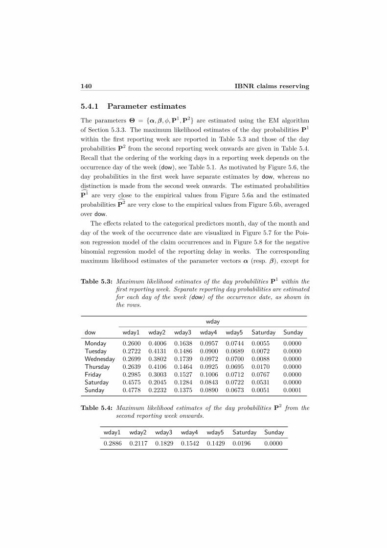
140 IBNR claims reserving
5.4.1 Parameter estimates
The parameters Θ = {α,β, φ, P1, P2} are estimated using the EM algorithmof Section 5.3.3. The maximum likelihood estimates of the day probabilities P1
within the first reporting week are reported in Table 5.3 and those of the dayprobabilities P2 from the second reporting week onwards are given in Table 5.4.Recall that the ordering of the working days in a reporting week depends on theoccurrence day of the week (dow), see Table 5.1. As motivated by Figure 5.6, theday probabilities in the first week have separate estimates by dow, whereas nodistinction is made from the second week onwards. The estimated probabilitiesP1 are very close to the empirical values from Figure 5.6a and the estimatedprobabilities P2 are very close to the empirical values from Figure 5.6b, averagedover dow.
The effects related to the categorical predictors month, day of the month andday of the week of the occurrence date are visualized in Figure 5.7 for the Pois-son regression model of the claim occurrences and in Figure 5.8 for the negativebinomial regression model of the reporting delay in weeks. The correspondingmaximum likelihood estimates of the parameter vectors α (resp. β), except for
Table 5.3: Maximum likelihood estimates of the day probabilities P1 within thefirst reporting week. Separate reporting day probabilities are estimatedfor each day of the week (dow) of the occurrence date, as shown inthe rows.
wdaydow wday1 wday2 wday3 wday4 wday5 Saturday SundayMonday 0.2600 0.4006 0.1638 0.0957 0.0744 0.0055 0.0000Tuesday 0.2722 0.4131 0.1486 0.0900 0.0689 0.0072 0.0000Wednesday 0.2699 0.3802 0.1739 0.0972 0.0700 0.0088 0.0000Thursday 0.2639 0.4106 0.1464 0.0925 0.0695 0.0170 0.0000Friday 0.2985 0.3003 0.1527 0.1006 0.0712 0.0767 0.0000Saturday 0.4575 0.2045 0.1284 0.0843 0.0722 0.0531 0.0000Sunday 0.4778 0.2232 0.1375 0.0890 0.0673 0.0051 0.0001
Table 5.4: Maximum likelihood estimates of the day probabilities P2 from thesecond reporting week onwards.
wday1 wday2 wday3 wday4 wday5 Saturday Sunday0.2886 0.2117 0.1829 0.1542 0.1429 0.0196 0.0000
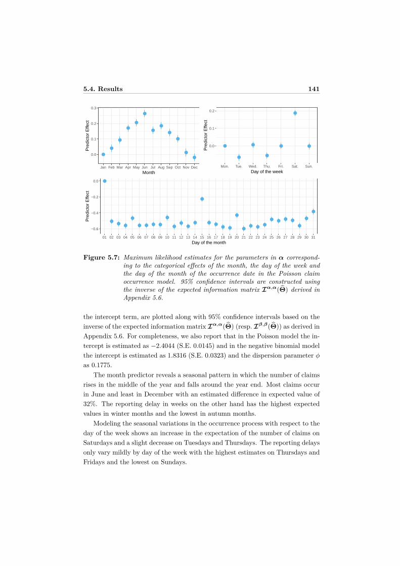
5.4. Results 141
●
●
●
●
●
●
●
●
●
●
●
●0.0
0.1
0.2
0.3
Jan Feb Mar Apr May Jun Jul Aug Sep Oct Nov Dec
Month
Pre
dict
or E
ffect
●
●●
●
●
●
●0.0
0.1
0.2
Mon. Tue. Wed. Thu. Fri. Sat. Sun.
Day of the week
Pre
dict
or E
ffect
●
●●
●
●
● ● ● ●
●
●●
●●
●
●●
● ●
●
●● ●
●
● ●● ●
●
●
●
−0.6
−0.4
−0.2
0.0
01 02 03 04 05 06 07 08 09 10 11 12 13 14 15 16 17 18 19 20 21 22 23 24 25 26 27 28 29 30 31
Day of the month
Pre
dict
or E
ffect
Figure 5.7: Maximum likelihood estimates for the parameters in α correspond-ing to the categorical effects of the month, the day of the week andthe day of the month of the occurrence date in the Poisson claimoccurrence model. 95% confidence intervals are constructed usingthe inverse of the expected information matrix Iα,α(Θ) derived inAppendix 5.6.
the intercept term, are plotted along with 95% confidence intervals based on theinverse of the expected information matrix Iα,α(Θ) (resp. Iβ,β(Θ)) as derived inAppendix 5.6. For completeness, we also report that in the Poisson model the in-tercept is estimated as −2.4044 (S.E. 0.0145) and in the negative binomial modelthe intercept is estimated as 1.8316 (S.E. 0.0323) and the dispersion parameter φ
as 0.1775.The month predictor reveals a seasonal pattern in which the number of claims
rises in the middle of the year and falls around the year end. Most claims occurin June and least in December with an estimated difference in expected value of32%. The reporting delay in weeks on the other hand has the highest expectedvalues in winter months and the lowest in autumn months.
Modeling the seasonal variations in the occurrence process with respect to theday of the week shows an increase in the expectation of the number of claims onSaturdays and a slight decrease on Tuesdays and Thursdays. The reporting delaysonly vary mildly by day of the week with the highest estimates on Thursdays andFridays and the lowest on Sundays.
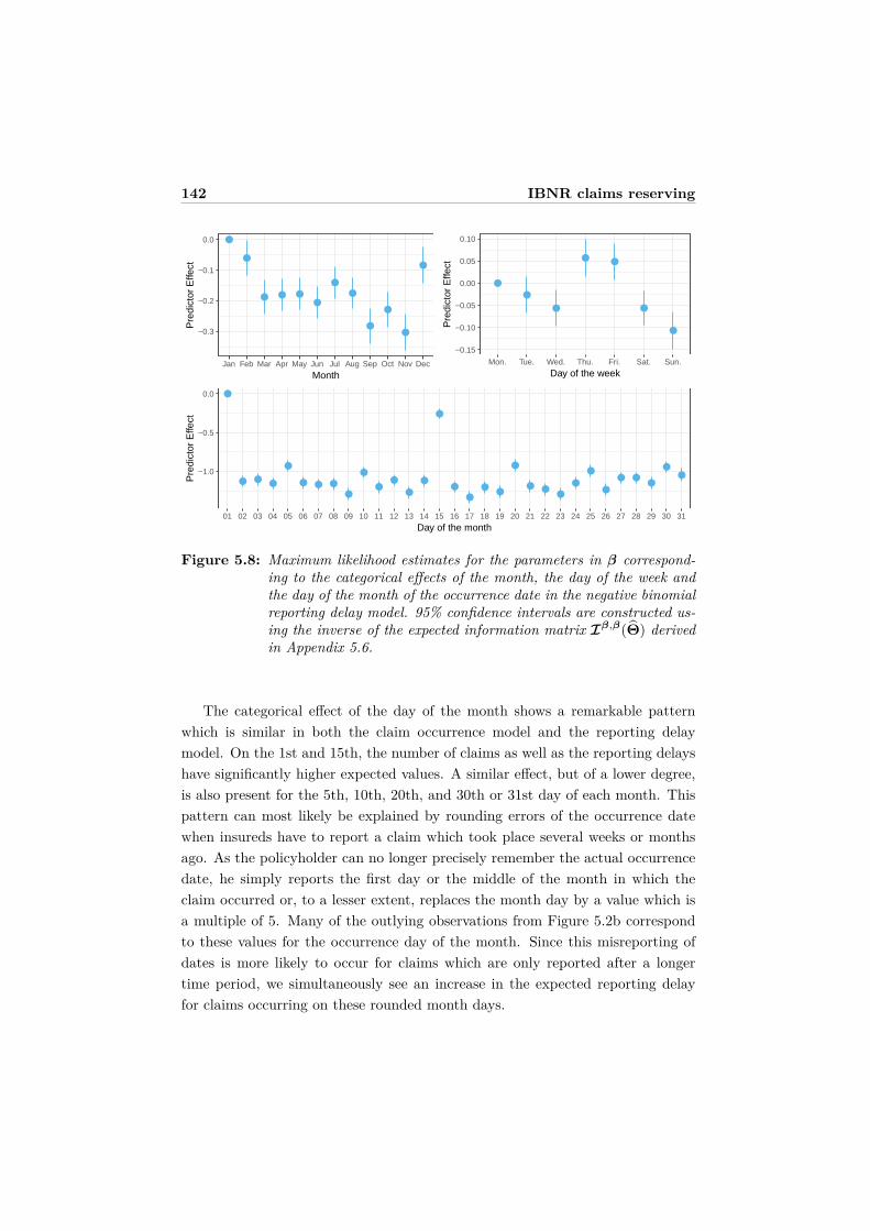
142 IBNR claims reserving
●
●
● ● ●
●
●
●
●
●
●
●
−0.3
−0.2
−0.1
0.0
Jan Feb Mar Apr May Jun Jul Aug Sep Oct Nov Dec
Month
Pre
dict
or E
ffect
●
●
●
●
●
●●
−0.15
−0.10
−0.05
0.00
0.05
0.10
Mon. Tue. Wed. Thu. Fri. Sat. Sun.
Day of the week
Pre
dict
or E
ffect
●
● ●●
●
● ● ●
●
●
●●
●
●
●
●
●
●●
●
● ●●
●
●
●
● ●●
●●−1.0
−0.5
0.0
01 02 03 04 05 06 07 08 09 10 11 12 13 14 15 16 17 18 19 20 21 22 23 24 25 26 27 28 29 30 31
Day of the month
Pre
dict
or E
ffect
Figure 5.8: Maximum likelihood estimates for the parameters in β correspond-ing to the categorical effects of the month, the day of the week andthe day of the month of the occurrence date in the negative binomialreporting delay model. 95% confidence intervals are constructed us-ing the inverse of the expected information matrix Iβ,β(Θ) derivedin Appendix 5.6.
The categorical effect of the day of the month shows a remarkable patternwhich is similar in both the claim occurrence model and the reporting delaymodel. On the 1st and 15th, the number of claims as well as the reporting delayshave significantly higher expected values. A similar effect, but of a lower degree,is also present for the 5th, 10th, 20th, and 30th or 31st day of each month. Thispattern can most likely be explained by rounding errors of the occurrence datewhen insureds have to report a claim which took place several weeks or monthsago. As the policyholder can no longer precisely remember the actual occurrencedate, he simply reports the first day or the middle of the month in which theclaim occurred or, to a lesser extent, replaces the month day by a value which isa multiple of 5. Many of the outlying observations from Figure 5.2b correspondto these values for the occurrence day of the month. Since this misreporting ofdates is more likely to occur for claims which are only reported after a longertime period, we simultaneously see an increase in the expected reporting delayfor claims occurring on these rounded month days.
5.4. Results 143
5.4.2 Prediction of IBNR claim counts
Besides providing insight in the claim occurrence process, the main goal of ourmodel is to estimate the number of IBNR claims. In our setting, the IBNR claimsare those with occurrence date in between January 2000 and August 2004 thathave only been reported after the evaluation date, August 31, 2004. We knowthere are 2052 such IBNR claims present in the full data set until August 2009of which we know the corresponding occurrence date and reporting delay, seethe lower triangle in Figure 5.3. These data are used to assess the out-of-samplepredictive performance.
Based on the fitted model where τ corresponds to August 31, 2004, the totalnumber of IBNR claims is estimated as N IBNR = 2066.03, which is very closeto the actual count. Moreover, the distributional assumptions of our model canbe used to provide a 95% prediction interval given by [1977, 2156], see Section5.3.5. Furthermore, since the model is defined on a daily level, the total IBNRprediction can be divided into daily forecasts by occurrence date and by reportingdate. This allows insurers to get a refined projection of the expected number ofIBNR claims according to their occurrence time points and their future reportingtimes. To illustrate this strong point of our model, we predict the IBNR claimcounts by occurrence dates in Figure 5.9 and by reporting dates in Figure 5.10.
In Figure 5.9a we plot point estimates and 95% prediction intervals for N IBNRt
with t corresponding to occurrences dates in between July 1, 2004, and August31, 2004, i.e. the last two months from our training period. The predictionsfollow the same trend as the actual IBNR claim counts derived from the full dataset until August 2009. In particular, we notice for instance how IBNR claimsare elevated on the first day and middle of each month, in line with our earlierfindings. In Figure 5.9b (resp. Figure 5.9c) we group the occurrence dates byweeks (resp. months) prior to the evaluation date and show the IBNR claim countpredictions corresponding to the past 26 weeks (resp. 12 months). We notice how,also over longer time spans, the predictions by occurrence week or month followthe pattern observed in the actual IBNR counts.
In Figure 5.10 we disperse the total predicted IBNR claim count according tothe date on which the IBNR claims will be reported to the insurer. It means wenow focus on estimating
∑τt=1 Nt,ρ−t for ρ = τ + 1, τ + 2, . . ., i.e. the number of
IBNR claims reported on day 1, 2, . . . of the out-of-sample period. This forms anappealing way to use our model in practice as it gives the insurer a refined viewon the reporting times of the IBNR claims. The predictions on a daily level inFigure 5.10a range from September 1, 2004, until November 7, 2004 and are again
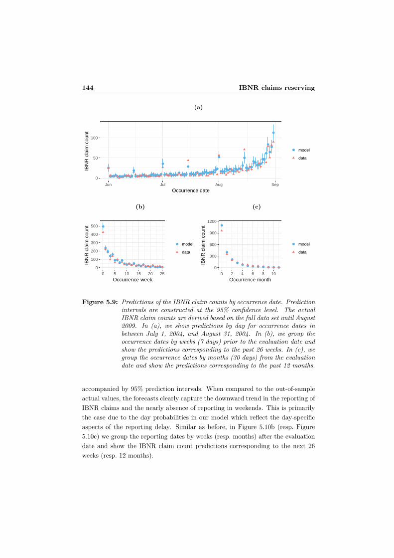
144 IBNR claims reserving
(a)
●
●●●●●●●●
●●●●●
●
●●●●●●●●●●●●●●●
●
●●●●
●●●●●
●●●●
●
●●●●●
●●●●●●●●●
●●
●
●●●●
●●●●
●●●●
●
●
●●●●
●●●●●
●●
●
●
●
●
●
0
50
100
Jun Jul Aug Sep
Occurrence date
IBN
R c
laim
cou
nt
● model
data
(b)
●
●
●
●●
● ●●
●
● ● ●●
●● ● ●
●● ● ●
●● ● ● ●0
100
200
300
400
500
0 5 10 15 20 25
Occurrence week
IBN
R c
laim
cou
nt
● model
data
(c)
●
●
●
●● ● ● ● ● ● ● ●0
300
600
900
1200
0 2 4 6 8 10
Occurrence month
IBN
R c
laim
cou
nt
● model
data
Figure 5.9: Predictions of the IBNR claim counts by occurrence date. Predictionintervals are constructed at the 95% confidence level. The actualIBNR claim counts are derived based on the full data set until August2009. In (a), we show predictions by day for occurrence dates inbetween July 1, 2004, and August 31, 2004. In (b), we group theoccurrence dates by weeks (7 days) prior to the evaluation date andshow the predictions corresponding to the past 26 weeks. In (c), wegroup the occurrence dates by months (30 days) from the evaluationdate and show the predictions corresponding to the past 12 months.
accompanied by 95% prediction intervals. When compared to the out-of-sampleactual values, the forecasts clearly capture the downward trend in the reporting ofIBNR claims and the nearly absence of reporting in weekends. This is primarilythe case due to the day probabilities in our model which reflect the day-specificaspects of the reporting delay. Similar as before, in Figure 5.10b (resp. Figure5.10c) we group the reporting dates by weeks (resp. months) after the evaluationdate and show the IBNR claim count predictions corresponding to the next 26weeks (resp. 12 months).
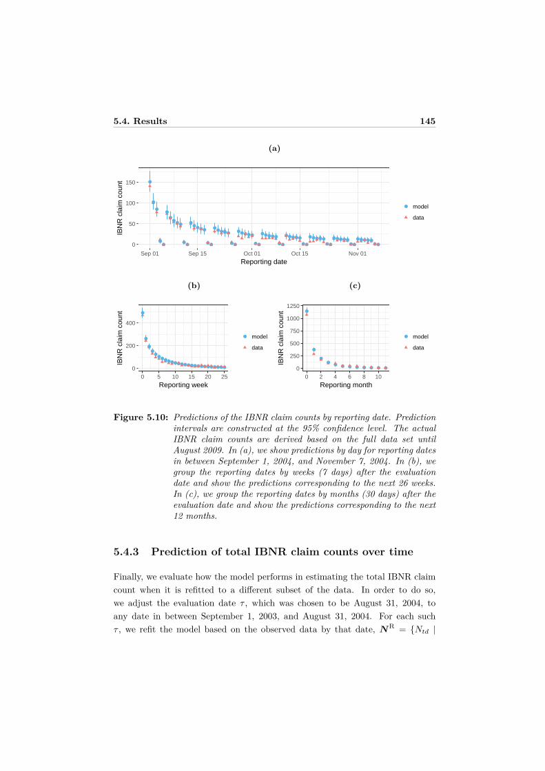
5.4. Results 145
(a)
●
●
●
●●
●
●●
● ●
●●
●●
● ● ●
● ●
●● ● ● ●
● ●
● ● ● ● ●
● ●
● ● ● ● ●
● ●
● ● ● ● ●
● ●
● ● ● ● ●
● ●
● ● ● ● ●
● ●
● ● ● ● ●● ●0
50
100
150
Sep 01 Sep 15 Oct 01 Oct 15 Nov 01
Reporting date
IBN
R c
laim
cou
nt
● model
data
(b)
●
●
●
●●
●● ● ● ● ● ● ● ● ● ● ● ● ● ● ● ● ● ● ● ●0
200
400
0 5 10 15 20 25
Reporting week
IBN
R c
laim
cou
nt
● model
data
(c)
●
●
●●
● ● ● ● ● ● ● ●0
250
500
750
1000
1250
0 2 4 6 8 10
Reporting month
IBN
R c
laim
cou
nt
● model
data
Figure 5.10: Predictions of the IBNR claim counts by reporting date. Predictionintervals are constructed at the 95% confidence level. The actualIBNR claim counts are derived based on the full data set untilAugust 2009. In (a), we show predictions by day for reporting datesin between September 1, 2004, and November 7, 2004. In (b), wegroup the reporting dates by weeks (7 days) after the evaluationdate and show the predictions corresponding to the next 26 weeks.In (c), we group the reporting dates by months (30 days) after theevaluation date and show the predictions corresponding to the next12 months.
5.4.3 Prediction of total IBNR claim counts over time
Finally, we evaluate how the model performs in estimating the total IBNR claimcount when it is refitted to a different subset of the data. In order to do so,we adjust the evaluation date τ , which was chosen to be August 31, 2004, toany date in between September 1, 2003, and August 31, 2004. For each suchτ , we refit the model based on the observed data by that date, NR = {Ntd |
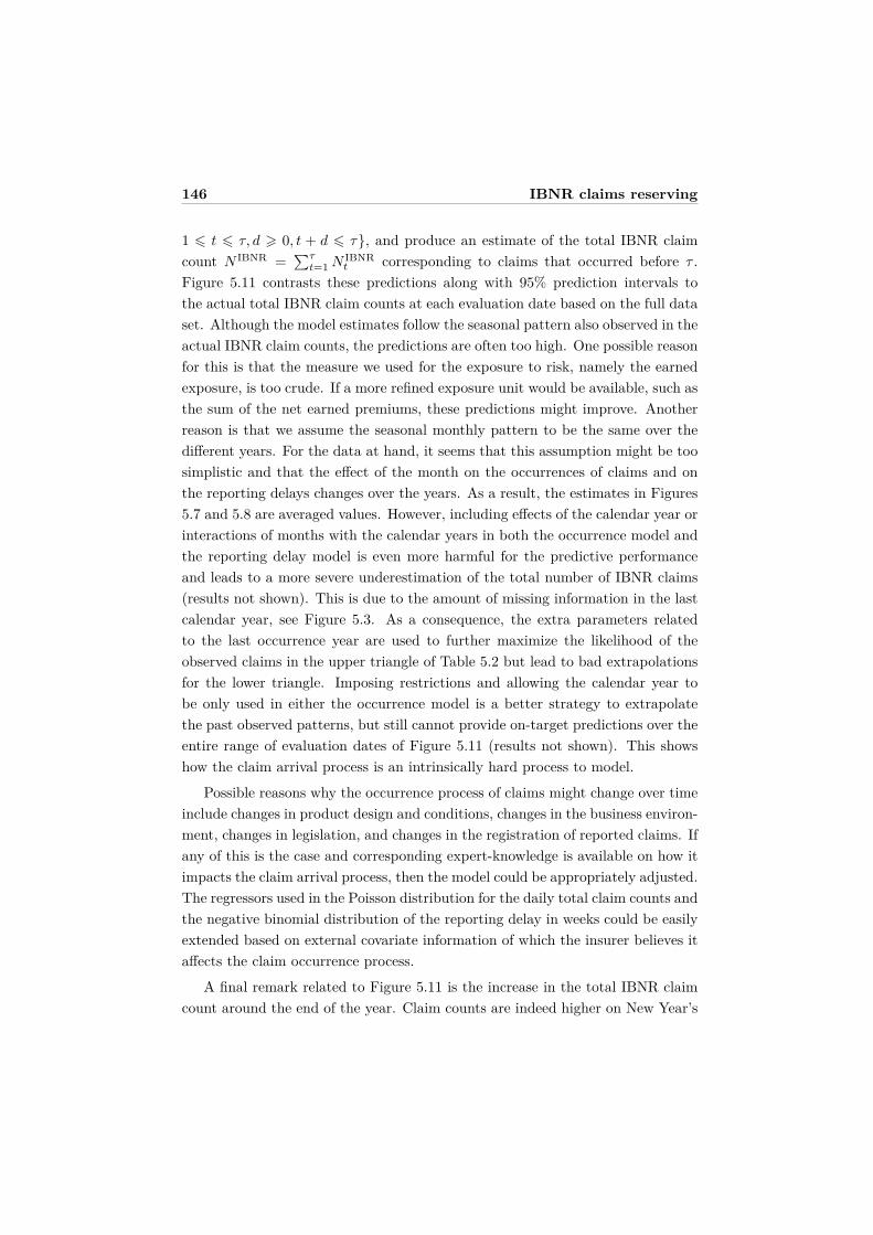
146 IBNR claims reserving
1 6 t 6 τ, d > 0, t + d 6 τ}, and produce an estimate of the total IBNR claimcount N IBNR =
∑τt=1 N IBNR
t corresponding to claims that occurred before τ .Figure 5.11 contrasts these predictions along with 95% prediction intervals tothe actual total IBNR claim counts at each evaluation date based on the full dataset. Although the model estimates follow the seasonal pattern also observed in theactual IBNR claim counts, the predictions are often too high. One possible reasonfor this is that the measure we used for the exposure to risk, namely the earnedexposure, is too crude. If a more refined exposure unit would be available, such asthe sum of the net earned premiums, these predictions might improve. Anotherreason is that we assume the seasonal monthly pattern to be the same over thedifferent years. For the data at hand, it seems that this assumption might be toosimplistic and that the effect of the month on the occurrences of claims and onthe reporting delays changes over the years. As a result, the estimates in Figures5.7 and 5.8 are averaged values. However, including effects of the calendar year orinteractions of months with the calendar years in both the occurrence model andthe reporting delay model is even more harmful for the predictive performanceand leads to a more severe underestimation of the total number of IBNR claims(results not shown). This is due to the amount of missing information in the lastcalendar year, see Figure 5.3. As a consequence, the extra parameters relatedto the last occurrence year are used to further maximize the likelihood of theobserved claims in the upper triangle of Table 5.2 but lead to bad extrapolationsfor the lower triangle. Imposing restrictions and allowing the calendar year tobe only used in either the occurrence model is a better strategy to extrapolatethe past observed patterns, but still cannot provide on-target predictions over theentire range of evaluation dates of Figure 5.11 (results not shown). This showshow the claim arrival process is an intrinsically hard process to model.
Possible reasons why the occurrence process of claims might change over timeinclude changes in product design and conditions, changes in the business environ-ment, changes in legislation, and changes in the registration of reported claims. Ifany of this is the case and corresponding expert-knowledge is available on how itimpacts the claim arrival process, then the model could be appropriately adjusted.The regressors used in the Poisson distribution for the daily total claim counts andthe negative binomial distribution of the reporting delay in weeks could be easilyextended based on external covariate information of which the insurer believes itaffects the claim occurrence process.
A final remark related to Figure 5.11 is the increase in the total IBNR claimcount around the end of the year. Claim counts are indeed higher on New Year’s
5.5. Conclusions and outlook 147
●
●
●
●●
●
●
●
●●
●●
●
●
●
●
●●●
●
●
●
●
●●●
●
●
●
●●
●●
●
●
●
●
●●●
●
●
●
●●●●
●
●
●
●
●●●
●
●
●
●
●●●
●
●
●
●
●●●
●
●
●
●●
●●
●
●
●
●
●●●
●
●
●
●●●●
●
●●
●
●●●
●
●
●
●●●●
●
●
●
●●●●
●
●
●
●●●●
●
●
●
●●●●
●
●
●
●●●●
●
●
●
●●●●
●
●
●●●●●
●
●
●
●●●●
●
●
●
●●●●
●
●
●
●●●●
●
●
●
●●●●
●
●
●
●●●●
●
●●
●●●●
●
●
●
●●●●
●
●
●
●
●●●
●
●
●
●●●●
●
●
●
●●
●●
●
●
●
●●●●
●
●
●
●●●●
●
●
●
●
●●●
●
●
●
●●●●
●
●
●
●●●●
●
●
●
●●●●
●
●
●
●
●●●
●
●
●
●●●●
●
●
●●
●●●
●
●
●
●
●●●
●
●
●●
●
●●
●
●
●
●
●●●
●
●
●
●●●
●
●
●
●
●
●●●
●
●
●
●
●●●
●
●
●
●
●●●
●
●
●
●
●●●
●
●
●
●
●●●
●
●
●
●
●●●
●
●
●
●
●
●●
●
●
●
●●●●
●
●
●
●
1500
1750
2000
2250
Oct 2003 Jan 2004 Apr 2004 Jul 2004
Evaluation date
IBN
R c
laim
cou
nt
● model
data
Figure 5.11: Predictions of the total IBNR claim counts for varying evaluationdates τ in between September 1, 2003, and August 31, 2004. Pre-diction intervals are constructed at the 95% confidence level. Theactual total IBNR claim counts are derived based on the full dataset until August 2009.
Eve and New Year as can be seen from Figure 5.2b. The model can incorporatethis aspect using designated dummy indicators in the regression models, but thiswould not completely make the IBNR predictions at the end of the year in linewith the actual values (results not shown). This is due to the fact that theinsurance company is closed around the holidays, preventing any claims frombeing reported at that time. Tackling this issue would require us to adjust theday-specific probabilities to take the absence of reporting on holidays into account,which is not straightforward to do under the model assumptions of Section 5.3.2.For this reason, it is advisable not to estimate the number of IBNR claims exactlyon the first or last day of the year.
5.5 Conclusions and outlook
We propose a new technique to model the claim arrival process on a daily basisin order to estimate the number of IBNR claim counts. The method uses regres-sion models for count data for the occurrence of claims and their correspondingreporting delays. The main idea introduced in this work is to treat the righttruncation of the reporting delays as a type of missing data. Applying the EMalgorithm strongly simplifies maximum likelihood estimation as it allows for theuse of standard statistical software to fit the regression models. We investigate
148 IBNR claims reserving
the performance of our micro-level IBNR reserving method in a case study witha European portfolio of general liability insurance policies for private individuals.The presented model provides a better understanding of the claim arrival processand can be used to predict IBNR claims on a daily level.
We indicate some possible directions for future research. First of all, we wouldlike to stress that the provided estimation framework involving the EM algorithmcan be applied to different models in this context. This provides a more desir-able alternative over the ad hoc methods or two-step approaches used earlier inactuarial literature. The essence of the estimation procedure described in Section5.3.3 would remain the same.
A direct extension of the model presented in this chapter would be to introducea multinomial logistic regression model for the day probabilities within a reportingweek shown in Figure 5.6. Incorporating covariate information would allow us tomodel possible evolutions of these reporting day probabilities over time. If say,for instance, in more recent years claims are also being reported on Sundaysthrough online reporting the day-specific probabilities would be able to adapt.This would be easily implemented because the EM algorithm relies on completedata computations which enables using a statistical software package to fit themultinomial logit model.
It would also be interesting to explore different distributional assumptions forthe daily total claim counts and the reporting delay distribution in weeks. Thereporting delay can be easily altered within the given framework to, for instance, azero-inflated or hurdle distribution or a more heavy-tailed distribution. Relaxingthe Poisson assumption for the daily total claim counts is also feasible but mightcomplicate the E-step in which we now relied on the thinning property of Poissondistributions. The EM framework is however compatible with latent underlyingprocesses affecting the occurrence of claims such as hidden Markov models orshot noise process (see e.g. Badescu et al., 2016a; Avanzi et al., 2016). Anotherpromising approach would be to investigate how time series models for counts (seeJung and Tremayne, 2011, for an overview) could be introduced in this setting.
5.6 Appendix: Derivation of the asymptotic va-riance-covariance matrix
Covariance matrix with respect to α The asymptotic covariance matrixof the MLE α can be estimated by the inverse of the submatrix of the observed
5.6. Appendix: Derivation of the asymptotic variance-covariancematrix 149
information matrix related to α, evaluated at Θ = Θ. Using relationship (5.13)between the incomplete data, complete data and missing information matrices,we have that
Iα,α(Θ;NR) = − ∂2
∂α∂α′ logL(Θ;NR) = Iα,αc (Θ;NR)− Iα,α
m (Θ;NR) .
The subvector of the complete data score statistic related to α is equal to
Sαc (Θ;N) = ∂
∂αlogLc(Θ;N)
= ∂
∂α
[−
τ∑t=1
et exp(x′tα) +
τ∑t=1
Nt(log(et) + x′tα)]
= −τ∑
t=1et exp(x′
tα)xt +τ∑
t=1Ntxt .
The missing information matrix with respect to α can be derived using (5.14) as
Iα,αm (Θ;NR) = Cov
[Sα
c (Θ;N) |NR; Θ]
= Cov[−
τ∑t=1
et exp(x′tα)xt +
τ∑t=1
Ntxt
∣∣∣∣∣NR; Θ]
= Cov[
τ∑t=1
Ntxt
∣∣∣∣∣NR; Θ]
= Cov[
τ∑t=1
( ∞∑d=τ−t+1
Ntd
)xt
∣∣∣∣∣NR; Θ]
=τ∑
t=1λtp
IBNRt xtx
′t , (5.16)
where we use the assumption that the daily total claim counts are independentlyPoisson distributed. Furthermore, we compute
Iα,αc (Θ;N) = − ∂2
∂α∂α′ logL(Θ;NR)
= − ∂
∂αSα
c (Θ;N)
=τ∑
t=1et exp(x′
tα)xtx′t , (5.17)
150 IBNR claims reserving
which does not depend on N such that
Iα,αc (Θ;NR) = E
[Iα,α
c (Θ;N) |NR; Θ]
= Iα,αc (Θ;N) ,
and
Iα,αc (Θ) = E [Iα,α
c (Θ;N) | Θ] = Iα,αc (Θ;N) .
By combing (5.16) and (5.17), evaluated at Θ = Θ, we thus find that
Iα,α(Θ;NR) = Iα,αc (Θ;NR)− Iα,α
m (Θ;NR)
=τ∑
t=1et exp(x′
tα)xtx′t −
τ∑t=1
λt pIBNRt xtx
′t
=τ∑
t=1λt pR
t xtx′t , (5.18)
which does not depend on the observed data NR and hence also equals Iα,α(Θ).Its inverse estimates the asymptotic covariance matrix of the MLE α. The missinginformation principle applied to the parameters of the Poisson regression modelfor the daily claim occurrences has a very intuitive interpretation: the observedinformation (5.18) related to the observed daily claim counts NR
t equals the com-plete information (5.17) related to the total daily claim counts Nt minus themissing information (5.16) related to the IBNR daily claim counts N IBNR
t .
Covariance matrix with respect to β Similarly for β, we use the relation
Iβ,β(Θ;NR) = − ∂2
∂β∂β′ logL(Θ;NR)
= Iβ,βc (Θ;NR)− Iβ,β
m (Θ;NR) . (5.19)
The score vector associated to β is given by
Sβc (Θ;N) = ∂
∂βlogLc(Θ;N)
=τ∑
t=1
∞∑w=0
( 6∑d=0
Nt,7w+d
)∂
∂βlog(pW
tw
)where
∂
∂βlog(pW
tw
)= ∂
∂β[wz′
tβ − (φ + w) log(φ + exp(z′tβ))]
5.6. Appendix: Derivation of the asymptotic variance-covariancematrix 151
= wzt − (φ + w) exp(z′tβ)zt
φ + exp(z′tβ)
= φ(w − exp(z′tβ))
φ + exp(z′tβ) zt .
Its conditional covariance is the missing information matrix related to β,
Iβ,βm (Θ;NR) = Cov
[Sβ
c (Θ;N) |NR; Θ]
=τ∑
t=1
∞∑w=0
∑d=0,...,6
7w+d>τ−t
λtpt,7w+d
φ2(w − exp(z′tβ))2
(φ + exp(z′tβ))2
ztz′t .
(5.20)
Moreover, we calculate
Iβ,βc (Θ;N) = − ∂2
∂β∂β′ logL(Θ;NR)
= − ∂
∂βSβ
c (Θ;N)
= −τ∑
t=1
∞∑w=0
( 6∑d=0
Nt,7w+d
)∂2
∂β∂β′ log(pW
tw
)(5.21)
where
∂2
∂β∂β′ log(pW
tw
)= ∂
∂β
[φ(w − exp(z′
tβ))φ + exp(z′
tβ) zt
]= −φ(φ + exp(z′
tβ)) exp(z′tβ)− φ(w − exp(z′
tβ)) exp(z′tβ)
(φ + exp(z′tβ))2 ztz
′t
= −φ(φ + w) exp(z′tβ)
(φ + exp(z′tβ))2 ztz
′t .
On substituting (5.20) and (5.21) into (5.19), we then have that
Iβ,β(Θ;NR) = Iβ,βc (Θ;NR)− Iβ,β
m (Θ;NR)
=τ∑
t=1
( ∞∑w=0
( 6∑d=0
Nt,7w+d
)φ(φ + w) exp(z′
tβ)(φ + exp(z′
tβ))2
)ztz
′t
−τ∑
t=1
∞∑w=0
∑d=0,...,6
7w+d>τ−t
λt pt,7w+d
φ2(w − exp(z′tβ))2
(φ + exp(z′tβ))2
ztz′t

152 IBNR claims reserving
with Nt,7w+d defined as in (5.8) using the MLE Θ. Its expectation with respectto the observed data NR is given by
Iβ,β(Θ) = Iβ,βc (Θ)− E
[Iβ,β
m (Θ;NR)∣∣∣ Θ]
=τ∑
t=1
( ∞∑w=0
λt pWtw
φ(φ + w) exp(z′tβ)
(φ + exp(z′tβ))2
)ztz
′t
−τ∑
t=1
∞∑w=0
∑d=0,...,6
7w+d>τ−t
λt pt,7w+d
φ2(w − exp(z′tβ))2
(φ + exp(z′tβ))2
ztz′t .
Either the inverse of Iβ,β(Θ;NR) or the inverse of Iβ,β(Θ) can be used toestimated the asymptotic covariance matrix of the MLE α.
Chapter 6
Outlook
By careful analysis of the available data using proper statistical techniques, insur-ance companies can improve the predictive power of their pricing and reservingtools and achieve a better understanding, measurement and management of therisks they are exposed to. We strongly believe that our proposed techniques in thecontext of loss reserving, telematics insurance and claims reserving may lead tobetter actuarial practices. This chapter concludes our work by presenting severalsuggestions for future research related to these topics.
The developed methodology can also be applied to other areas where similardata are collected and analyzed. The expected impact is broader than only onactuarial science with potential applications in, for instance, econometrics (e.g. theunemployment duration data from Section 2.5.2), geology (e.g. the Old faithfulgeyser data from Section 3.5.2 and the use of compositional predictors in Chapter4) and biostatistics (e.g. the mastitis study from Section 3.5.3 and the modelingof reporting delays in infectious disease data using the approach for IBNR claimsreserving of Chapter 5).
6.1 Further developments in loss modeling
In Chapter 2, we develop an estimation procedure using the EM algorithm that isable to fit a mixture of Erlang distributions to censored and truncated data. Theflexibility of mixtures of Erlang distributions and the effectiveness of the proposedfitting algorithm is demonstrated using several simulated and real data sets. Inparticular, for the left truncated Secura Re data set a mixture of two Erlang com-ponents adequately represents the moderately heavy-tailed claim sizes. In the
153
154 Outlook
example of Section 2.5.4, we illustrate its limitations when data are generatedfrom a generalized Pareto distribution with extreme value index equal to one,which expresses a very heavy tail. Because mixtures of Erlangs have asymptoti-cally exponential tails, which are lighter, in such example there is no parsimoniousmodel possible using such mixtures. Erlang components in a mixture are not ableto extrapolate the heaviness in the tail and instead behave similar to an empiricaldistribution in the upper tail. However, this behavior might be undesirable froma risk measurement perspective. An accurate description of the upper tail of theclaim size distribution is important to safeguard the insurance company againstextreme losses that might jeopardize its solvency. Reynkens et al. (2016) addressthis issue by considering a splicing model where a mixture of Erlang distributionsis used for the body of the distribution and a Pareto distribution for the tail. Aglobal fit results, which combines the flexibility of the mixture of Erlangs distribu-tion to model light and moderate losses with the ability of the Pareto distributionto model extreme values.
This idea can be extended to the multivariate setting from Chapter 3 in or-der to provide a global fit strategy for heavy-tailed, dependent losses. The mostpromising approach is to combine the multivariate mixtures of Erlang distribu-tions (MME) with the multivariate generalized Pareto distribution (MGPD). TheMGPD class is proposed in Rootzen and Tajvidi (2006) and combines univariategeneralized Pareto distributions using a dependence structure to model the tailregions where at least one component of the vector is large. In such a multivariatesplicing model, an MME would be used to represent losses below a d-dimensionalsplicing point and an MGPD for losses that exceed the splicing point in at leastone dimension.
The definition of a (univariate and multivariate) mixture of Erlang distribu-tions can readily be generalized to include a discrete point mass at zero. Thisaccommodates common situations in practice when one explicitly wants to modelthe positive probability of a zero loss, i.e. when no loss has been incurred. Thepresented EM algorithm in Chapters 2 and 3 can straightforwardly be adapted tothis extension.
The selection of shape parameters for mixtures of Erlangs is based on itera-tively using the EM algorithm and comparing the fits based on AIC or BIC. Thealgorithms used to initialize, adjust and reduce the shape parameters performwell, but the strategy is computationally intensive and depends on the values ofthe initializing parameters M and s. It would be interesting to look into alter-native ways to approach the choice of the shapes which forms a computationally
6.2. Further developments in telematics insurance 155
unsolvable optimization problem over NM . In a recent effort, Yin and Lin (2016)propose the use of regularization techniques for univariate mixtures of Erlangs,inspired by the MSCAD penalized likelihood of Chen and Khalili (2008). How-ever, it still requires an initial choice for the shape set and introduces new tuningparameters.
In future research we aim to extend the mixtures of Erlangs framework towardsthe inclusion of predictor variables and introduce the flexibility of this approachin a regression context. Our idea is to translate the covariate information intothe mixing weights of the components in the mixture of Erlang distributions.The common scale parameter then remains the same for all observations, but theweights in the mixture become a function of the linear predictor including theavailable covariates. In the univariate setting, we suggest to model the weightsusing a cumulative logit model (also called a proportional odds model). Thismodel is used for ordinal dependent variables, which makes it a promising avenuein this setting since the mixing components have a natural ordering based on thevalue of the corresponding shape parameter. Introducing such a model for themixing weights leads to solving an additional regression model in each M-step ofthe EM algorithm in order to update the corresponding parameters used in theweight specifications. In the multivariate setting, there is no natural ordering ofthe shape parameter vectors and a multinomial logit model for the mixing weightscould be considered instead.
6.2 Further developments in telematics insurance
In Chapter 4, we investigate a Belgian telematics car insurance data set. Thegoal is to incorporate the telematics information to make better predictions onthe number of claims and to identify the relationship between the driving habitsand the accident risk. Compositional predictors are introduced to quantify andinterpret the effect of the driving habits on the riskiness. The analysis showsthat the use of this new type of data collected through telematics technologyleads to improved predictions in actuarial pricing. Moreover, moving towards carinsurance rating based on individual driving habits and style can resolve possiblediscrimination of basing the premium on proxies such as gender.
The novelty of telematics insurance calls for future research and requires aninterdisciplinary approach. From a business perspective, it would be interestingto evaluate how the proposed prediction model using telematics variables canimpact the pricing strategies and profitability of insurance companies. The cost
156 Outlook
effectiveness of usage-based insurance could be assessed, taking into account theimplementation cost of black box devices and related data management. Businessmodels need to be designed that generate value from pay-as-you-drive insurancefor both individuals and firms.
From the perspective of actuarial science and econometrics, telematics insur-ance is at the cross-road of a priori and a posteriori rating and demands a rethink-ing of common practices in both activities. This opens up new possibilities forfuture research on competitive adaptive pricing strategies. Premium structurescan be developed to more closely reflect the actual risk exposure and to adaptover time based on the observed driving behavior after the underwriting of thepolicy. Financial rewards along with personalized driving style feedback will givepolicyholders a high incentive to drive more responsible, thus minimizing risk andimproving road safety.
From a statistics and machine learning perspective, the most exciting futurechallenges lie in the analysis of telematics data on a more granular level. Telem-atics technology offers the possibility to collect real-time driving data via theblack box device installed in a car. Insurers however partner with telematicsdata providers who process the raw telematics data, enrich these using externaldata sources (e.g. road maps) and deliver structured, aggregated telematics in-formation. The daily summarized data we analyzed in Chapter 4 on how much,where and when the vehicle is driven forms a typical data setup in which insur-ance companies receive telematics data from such data providers. More extensivedata formats also include certain driving style scores based on speeding viola-tions, harsh braking, excessive accelerating, and cornering style. These kind ofUBI driving scores can be easily incorporated in the presented framework.
To obtain a more comprehensive view on the driving style, it is desirable tohave the raw telematics data in the form of streams of coordinates available (whichis not the case in our setting). Statistical analysis of these spatiotemporal data isa highly relevant direction for future research. The main difficulty is to transformthis high-frequency GPS location data into interpretable covariates describingcomplex driving patterns. Basic features that can be derived from GPS dataat every time point are the speed, difference in speed, acceleration, differencein acceleration and angular speed. It is important to also account for specificdriving contexts, such as road type, traffic situations and weather conditions.Using techniques from unsupervised learning and pattern recognition the goal isto classify different driving styles. In a next step, these driving style classes can beused as risk factors in claim count regression models to evaluate the effectiveness
6.3. Further developments in claims reserving 157
of the classification in assessing the accident risk. Insurers must carefully considerwhich of these sensor data-derived classifications constitute suitable rating factorsin usage-based car insurance pricing and to what extent they improve the qualityof predictions.
6.3 Further developments in claims reserving
In Chapter 5, we contribute to the micro-level loss reserving literature by formu-lating a regression framework to model the claims arrival process along with itsreporting delays on a daily level. The model can be used to predict the num-ber of daily future claim counts in order to set up adequate IBNR claim reserves.The proposed methodology can be further developed and applied to multiple othercase-studies, from different lines of business. The presented estimation frameworkusing the EM algorithm can also be employed in alternative claims reserving mod-els to obtain a joint estimation of both the occurrence and the reporting delaymodel parameters.
Several directions exist for future research in micro-level claims reserving. Themost important path is to focus on the payment process, from reporting untilsettlement of a claim. Modeling the dynamics of the individual development ofclaims forms the next necessary building block to extend our micro-level lossreserving technique and to estimate future cash flows.
Arjas (1989), Norberg (1993) and Norberg (1999) developed a mathematical,probabilistic framework for the development of individual claims in continuoustime. More recently, Antonio and Plat (2014) make this theory accessible toreserving practice by translating these probabilistic ideas to a statistical model inwhich estimation, inference and prediction is demonstrated on a real life data set.In their approach, hazard rates drive the time to events in the development of aclaim (e.g. a payment, or settlement) and a lognormal regression is used to modelintermediate payments corrected for inflation using a consumer price index.
Building upon the work of Antonio and Plat (2014), it would be interesting torelax the distributional assumptions made and to incorporate claim-specific infor-mation as covariates. Insurers’ data base systems contain detailed information onopen claims and their ongoing development: characteristics of the policy(holder),the accident, the (initial) case estimate (i.e. an expert judgment of the final claimamount), the reporting delay, the cumulative amount paid so far, etc. Traditionalreserving methods compress these large data sets into small run-off triangles andhereby ignore this detailed information. Micro-level loss reserving offers the op-

158 Outlook
portunity to instead use these claim-specific characteristics as predictive variables.This allows for a more realistic modeling of the development process which is ex-pected to result in more accurate estimates and forecasts.

List of Figures
2.1 Graphical comparison of the density of the fitted mixture of 3 Er-langs, the true underlying density (2.18) and the histogram of thegenerated data before censoring and truncation (left) and of thetruncated density of the fitted mixture of 3 Erlangs, the true trun-cated density and the histogram of the generated data after trun-cated and before censoring (right). . . . . . . . . . . . . . . . . . . 27
2.2 Graphical comparison of the survival function of the fitted mixtureof 8 Erlangs and the Kaplan-Meier estimator with 95% confidencebounds for the right-censored unemployment data. . . . . . . . . . 30
2.3 Graphical comparison of the truncated density of the fitted mixtureof 2 Erlangs and the histogram of the left-truncated claim sizes(left) and of the truncated survival function and the Kaplan-Meierestimator with 95% confidence bounds (right) for the Secura Redata set. . . . . . . . . . . . . . . . . . . . . . . . . . . . . . . . . . 32
2.4 QQ-plot of the empirical quantiles and the quantiles of the fittedmixture of 2 Erlangs with identity line (left) and log-log plot of theempirical truncated survival function and the truncated survivalfunction of the fitted Erlang mixture (right) for the Secura Re dataset. . . . . . . . . . . . . . . . . . . . . . . . . . . . . . . . . . . . . 32
2.5 Graphical comparison of the truncated density of the fitted mix-ture of 16 Erlangs and the histogram (left) and of the truncatedsurvival function and the Kaplan-Meier estimator with 95% confi-dence bounds (right) for the simulated generalized Pareto data upto the 95% empirical quantile. . . . . . . . . . . . . . . . . . . . . . 37
159
160 List of Figures
2.6 QQ-plot of the empirical quantiles and the quantiles of the fittedmixture of 16 Erlangs with identity line (left) and log-log plot ofthe empirical truncated survival function and the truncated sur-vival function of the fitted Erlang mixture (right) for the simulatedgeneralized Pareto data. . . . . . . . . . . . . . . . . . . . . . . . . 37
3.1 Simulated example: (a) scatterplot, (b) marginal quantile grid, (c)grid formed by multiplying the shapes (3.17) by the common scale(3.20) and (d) initial weight α
(0)r=(9,207) = 0.024. . . . . . . . . . . . 62
3.2 Scatterplot of the simulated data with an overlay of the fitted den-sity of the MME using a contour plot and heat map. In the mar-gins, we plot the marginal histograms with an overlay of the truedensities in blue and the fitted densities in red. In (a), we displaythe fit after initialization, in (b) after applying the EM algorithm afirst time, in (c) after applying the reduction step and in (d) afterapplying the adjustment and further reduction step. . . . . . . . . 64
3.3 BIC values when fitting an MME to the Old Faithful geyser data,starting from different values of the tuning parameters. The mini-mum BIC value is obtained for M = 10 and s = 90. . . . . . . . . 66
3.4 Graphical evaluation of the best-fitting MME to the Old Faithfulgeyser data. In (a), we display the scatterplot of the data with anoverlay of the fitted density using a contour plot and heat map.The margins show the marginal histograms with an overlay of thefitted densities in red. In (b), we compare the fitted density of thesum of the components and the histogram of the observed totalcycle times. . . . . . . . . . . . . . . . . . . . . . . . . . . . . . . . 67
3.5 Scatterplot matrix comparing the fitted four-dimensional MME tothe observed interval and right censored observations of the mastitisdata (infections by all bacteria). For more explanation, see Section3.5.3 . . . . . . . . . . . . . . . . . . . . . . . . . . . . . . . . . . . 70
4.1 (a) A schematic overview of the flow of information. (b) The num-ber of registered kilometers on each day on an aggregate, portfoliolevel for the telematics data observed between January 1, 2010 andDecember 31, 2014. The outliers by the turn of the year 2014,corresponding to a technical malfunction, are indicated as triangles. 82

List of Figures 161
4.2 Histogram of (a) the duration (in days) of the policy period (atmost one year) and (b) the driven distance (in 1000 km) duringthe policy period. (c) A graphical representation of the similaritiesand differences between the four predictor sets. . . . . . . . . . . . 86
4.3 Histograms and bar plots of the continuous and categorical policyvariables contained in the data set. The map in the lower rightdepicts the geographical information by showing the proportion ofinsureds per squared kilometer living in each of the different postalcodes in Belgium. The five class intervals have been created usingk-means clustering. . . . . . . . . . . . . . . . . . . . . . . . . . . . 87
4.4 Graphical illustration of the telematics variables contained in thedata set. For the yearly and average distance, we construct his-tograms. For the division of the driven distance by road types,time slots and week/weekend, we construct box plots of the rel-ative proportions. To highlight the dependencies intrinsic to thefact that the division in different categories sums to one, we plotprofile lines for 100 randomly selected observations in the data set. 88
4.5 Multiplicative response effects of the policy model terms of thetime-hybrid model. . . . . . . . . . . . . . . . . . . . . . . . . . . . 105
4.6 Multiplicative response effects of the telematics model terms of thetime-hybrid model. . . . . . . . . . . . . . . . . . . . . . . . . . . . 105
4.7 Multiplicative response effects of the model terms of the classicmodel. . . . . . . . . . . . . . . . . . . . . . . . . . . . . . . . . . . 113
4.8 Multiplicative response effects of the model terms of the telematicsmodel. . . . . . . . . . . . . . . . . . . . . . . . . . . . . . . . . . . 113
4.9 Multiplicative response effects of the policy model terms of themeter-hybrid model. . . . . . . . . . . . . . . . . . . . . . . . . . . 114
4.10 Multiplicative response effects of the telematics model terms of themeter-hybrid model. . . . . . . . . . . . . . . . . . . . . . . . . . . 114
4.11 Relative frequencies of the multiplicative response effects of themodel terms of the classic model. . . . . . . . . . . . . . . . . . . . 116
4.12 Relative frequencies of the multiplicative response effects of themodel terms of the telematics model. . . . . . . . . . . . . . . . . . 116
4.13 Relative frequencies of the multiplicative response effects of thepolicy model terms of the time-hybrid model. . . . . . . . . . . . . 117
4.14 Relative frequencies of the multiplicative response effects of thetelematics model terms of the time-hybrid model. . . . . . . . . . . 117

162 List of Figures
4.15 Relative frequencies of the multiplicative response effects of thepolicy model terms of the meter-hybrid model. . . . . . . . . . . . 118
4.16 Relative frequencies of the multiplicative response effects of thetelematics model terms of the meter-hybrid model. . . . . . . . . . 118
5.1 Time line representing the development of a single claim. . . . . . 121
5.2 From January 1, 2000 until August 31, 2004, we plot (a) the earnedexposure per day and (b) the number of claims occurring on thatday based on the full data set until August 2009. . . . . . . . . . . 125
5.3 Daily run-off triangle of claims with occurrence dates between Jan-uary 1, 2000 and August 31, 2004. The black line indicates theevaluation date, August 31, 2004. Only the claims in the uppertriangle depicted as blue dots are observed at the evaluation date.The remaining claims in the lower triangle depicted as red trianglesare the IBNR claims based on the full data set until August 2009and have to be predicted. . . . . . . . . . . . . . . . . . . . . . . . 126
5.4 Bar plot of the empirical reporting delay distribution in the first 4weeks for claims that occurred on (a) Monday, (b) Thursday and(c) Saturday between January 2000 and August 2004 and have beenreported before August 2009. . . . . . . . . . . . . . . . . . . . . . 127
5.5 Bar plot of the empirical reporting delay distribution in weeks andits negative binomial fit for the first 11 weeks in (a) and for thefirst year in (b) based on claims that occurred between January2000 and August 2004 and have been reported before August 2009. 128
5.6 Stacked bar plots of the empirical reporting delay day probabilitieswithin a reporting week according to the day of the week of theoccurrence date. Based on claims that occurred between January2000 and August 2004 and have been reported before August 2009,we show the empirical day probabilities during the first reportingweek in (a) and from the second reporting week onwards in (b).The ordering of the working days in a reporting week according tothe day of the week of the occurrence date is clarified in Table 5.1. 128
List of Figures 163
5.7 Maximum likelihood estimates for the parameters in α correspond-ing to the categorical effects of the month, the day of the week andthe day of the month of the occurrence date in the Poisson claimoccurrence model. 95% confidence intervals are constructed usingthe inverse of the expected information matrix Iα,α(Θ) derived inAppendix 5.6. . . . . . . . . . . . . . . . . . . . . . . . . . . . . . . 141
5.8 Maximum likelihood estimates for the parameters in β correspond-ing to the categorical effects of the month, the day of the weekand the day of the month of the occurrence date in the nega-tive binomial reporting delay model. 95% confidence intervals areconstructed using the inverse of the expected information matrixIβ,β(Θ) derived in Appendix 5.6. . . . . . . . . . . . . . . . . . . 142
5.9 Predictions of the IBNR claim counts by occurrence date. Pre-diction intervals are constructed at the 95% confidence level. Theactual IBNR claim counts are derived based on the full data setuntil August 2009. In (a), we show predictions by day for occur-rence dates in between July 1, 2004, and August 31, 2004. In (b),we group the occurrence dates by weeks (7 days) prior to the eval-uation date and show the predictions corresponding to the past 26weeks. In (c), we group the occurrence dates by months (30 days)from the evaluation date and show the predictions correspondingto the past 12 months. . . . . . . . . . . . . . . . . . . . . . . . . 144
5.10 Predictions of the IBNR claim counts by reporting date. Predictionintervals are constructed at the 95% confidence level. The actualIBNR claim counts are derived based on the full data set untilAugust 2009. In (a), we show predictions by day for reporting datesin between September 1, 2004, and November 7, 2004. In (b), wegroup the reporting dates by weeks (7 days) after the evaluationdate and show the predictions corresponding to the next 26 weeks.In (c), we group the reporting dates by months (30 days) after theevaluation date and show the predictions corresponding to the next12 months. . . . . . . . . . . . . . . . . . . . . . . . . . . . . . . . 145
5.11 Predictions of the total IBNR claim counts for varying evaluationdates τ in between September 1, 2003, and August 31, 2004. Pre-diction intervals are constructed at the 95% confidence level. Theactual total IBNR claim counts are derived based on the full dataset until August 2009. . . . . . . . . . . . . . . . . . . . . . . . . . 147


List of Tables
2.1 Demonstration of initialization and fitting procedure on the datagenerated from (18). Starting point is a mixture of 10 Erlangs.The initial spread factor s ranges from 1 to 10. The superscriptsin the last two columns represent the preference order according tothat information criterium. . . . . . . . . . . . . . . . . . . . . . . 26
2.2 Parameter estimates of the mixture of 3 Erlangs fitted to the cen-sored and truncated data with underlying density (2.18). . . . . . . 26
2.3 Results of the sensitivity analysis with respect to the level of cen-soring. For each value of p in the right censoring distribution (2.19),we generate 100 censoring samples and report the average censoringlevel and average performance measures of the best-fitting mixturesof Erlang distributions. . . . . . . . . . . . . . . . . . . . . . . . . . 29
2.4 Parameter estimates of the mixture of 8 Erlangs fitted to the right-censored unemployment data. . . . . . . . . . . . . . . . . . . . . . 30
2.5 Comparison of information criteria for the different models fittedto the right-censored unemployment data. . . . . . . . . . . . . . . 31
2.6 Parameter estimates of the mixture of 2 Erlangs fitted to the left-truncated claim sizes in the Secura Re data set. . . . . . . . . . . . 31
2.7 Non-parametric, Hill, GP and Mixture of Erlangs-based estimatesfor Π(R). . . . . . . . . . . . . . . . . . . . . . . . . . . . . . . . . 34
2.8 Non-parametric, Exp-Par and Mixture of Erlangs-based estimatesfor Π(R). . . . . . . . . . . . . . . . . . . . . . . . . . . . . . . . . 34
2.9 Parameter estimates of the mixture of 16 Erlangs fitted to thesimulated generalized Pareto data. . . . . . . . . . . . . . . . . . . 36
3.1 Parameter estimates of the MME with 11 mixture components fit-ted to the simulated data. . . . . . . . . . . . . . . . . . . . . . . . 65
165
166 List of Tables
3.2 BIC values and number of mixture components when fitting anMME to the Old Faithful geyser data, starting from different valuesof the tuning parameters. The minimum BIC value is underlinedand obtained for M = 10 and s = 90. . . . . . . . . . . . . . . . . . 66
3.3 Parameter estimates of the best-fitting MME with 15 mixture com-ponents fitted to the Old Faithful geyser data. . . . . . . . . . . . . 66
3.4 Parameter estimates of the best-fitting MME with four mixturecomponents fitted to the mastitis data (infections by all bacteria). 69
3.5 Estimates and 90% bootstrap confidence intervals for the bivariatemeasures of association Kendall’s τ and Spearman’s ρ based on thefitted MME for the mastitis data (infections by all bacteria). . . . 71
4.1 Description of the variables contained in the data set arising fromthe different sources of information. . . . . . . . . . . . . . . . . . . 83
4.2 Proper scoring rules for count data. . . . . . . . . . . . . . . . . . . 994.3 Variables contained in the best Poisson model for each of the pre-
dictor sets. The second column of each predictor set refers to themodel with the offset restriction for either time or meter. The bestNB models were identical to the best Poisson models. . . . . . . . 100
4.4 Model assessment of the best models according to AIC for eachof the four predictor sets under the Poisson model specification.The second row of each predictor set refers to the model with theoffset restriction for either time or meter. For each model we listthe effective degrees of freedom (EDF), Akaike information crite-rion (AIC) and 6 cross-validated proper scoring rules: logarithmic(logs), quadratic (qs), spherical (sphs), ranked probability (rps),Dawid-Sebastiani (dss), and squared error scores (ses). For AICand the proper scoring rules, the first column represents the valueand the second column the rank. . . . . . . . . . . . . . . . . . . . 102
4.5 Structural zero patterns for the division of meters in road types. . 1104.6 Structural zero patterns for the division of meters in time slots. . 1104.7 Structural zero patterns for the division of meters in week and
weekend. . . . . . . . . . . . . . . . . . . . . . . . . . . . . . . . . . 1114.8 Structural zero patterns for the division of the number of meters
in road types, time slots and week/weekend as recognized in theclaim count models. . . . . . . . . . . . . . . . . . . . . . . . . . . 111

List of Tables 167
4.9 Standard deviations of the effects on the predictor scale in the bestPoisson model for each of the predictor sets. The second columnof each predictor set refers to the model with the offset restrictionfor either time or meter. . . . . . . . . . . . . . . . . . . . . . . . . 115
5.1 Ordering of the working days in the week (wday) by the day of theweek (dow) of the occurrence date. wday3, for example, denotesthe third working day of the reporting week, which is Wednesdaywhen the claim occurred on Monday and a Monday when the claimoccurred on Thursday, and so on. . . . . . . . . . . . . . . . . . . . 129
5.2 Run-off triangle with daily claim counts. Only the claim counts inthe upper triangle are observed, whereas the claim counts in thelower triangle have to be predicted. . . . . . . . . . . . . . . . . . . 130
5.3 Maximum likelihood estimates of the day probabilities P1 withinthe first reporting week. Separate reporting day probabilities areestimated for each day of the week (dow) of the occurrence date,as shown in the rows. . . . . . . . . . . . . . . . . . . . . . . . . . . 140
5.4 Maximum likelihood estimates of the day probabilities P2 from thesecond reporting week onwards. . . . . . . . . . . . . . . . . . . . . 140


Bibliography
Aitchison, J. (1986). The statistical analysis of compositional data. Chapman andHall London.
Aitchison, J. and Kay, J. W. (2003). Possible solution of some essentialzero problems in compositional data analysis. In Thio-Henestrosa, S. andMartın-Fernandez, J. A., editors, Proceedings of CoDaWork’03, The 1st Com-positional Data Analysis Workshop. University of Girona.
Akaike, H. (1974). A new look at the statistical model identification. IEEETransactions on Automatic Control, 19(6):716–723.
Ampe, B., Goethals, K., Laevens, H., and Duchateau, L. (2012). Investigatingclustering in interval-censored udder quarter infection times in dairy cows usinga gamma frailty model. Preventive veterinary medicine, 106(3):251–257.
Antonio, K., Godecharle, E., and Oirbeek, R. V. (2016). A multi-state approachand flexible payment distributions for micro-level reserving in general insurance.Working paper AFI16106.
Antonio, K. and Plat, R. (2014). Micro–level stochastic loss reserving for generalinsurance. Scandinavian Actuarial Journal, 7:649–669.
Arjas, E. (1989). The claims reserving problem in non–life insurance: some struc-tural ideas. ASTIN Bulletin, 19(2):139–152.
Asmussen, S., Nerman, O., and Olsson, M. (1996). Fitting phase-type distribu-tions via the EM algorithm. Scandinavian Journal of Statistics, pages 419–441.
Assaf, D., Langberg, N. A., Savits, T. H., and Shaked, M. (1984). Multivariatephase-type distributions. Operations Research, 32(3):688–702.
169
170 BIBLIOGRAPHY
Avanzi, B., Wong, B., and Yang, X. (2016). A micro-level claim count model withoverdispersion and reporting delays. Insurance: Mathematics and Economics,71:1–14.
Ayuso, M., Guillen, M., and Perez-Marın, A. M. (2014). Time and distance to firstaccident and driving patterns of young drivers with pay-as-you-drive insurance.Accident Analysis & Prevention, 73:125–131.
Ayuso, M., Guillen, M., and Perez-Marın, A. M. (2016a). Telematics and genderdiscrimination: Some usage-based evidence on whether men’s risk of accidentsdiffers from women’s. Risks, 4(2):10.
Ayuso, M., Guillen, M., and Perez-Marın, A. M. (2016b). Using {GPS} data toanalyse the distance travelled to the first accident at fault in pay-as-you-driveinsurance. Transportation Research Part C: Emerging Technologies, 68:160 –167.
Azzalini, A. and Bowman, A. (1990). A look at some data on the old faithfulgeyser. Applied Statistics, pages 357–365.
Bacon Shone, J. (2003). Modelling structural zeros in compositional data. InThio-Henestrosa, S. and Martın-Fernandez, J. A., editors, Proceedings of CoDa-Work’03, The 1st Compositional Data Analysis Workshop. University of Girona.
Badescu, A., Gong, L., Lin, X. S., and Tang, D. (2015). Modeling correlatedfrequencies with applications in operational risk management. Journal of Op-erational Risk. forthcoming.
Badescu, A. L., Lin, X. S., and Tang, D. (2016a). A marked Cox model forthe number of IBNR claims: Estimation and application. Available at SSRN2747223.
Badescu, A. L., Lin, X. S., and Tang, D. (2016b). A marked Cox model forthe number of IBNR claims: Theory. Insurance: Mathematics and Economics,69:29–37.
Barcelo-Vidal, C., Martın-Fernandez, J. A., and Mateu-Figueras, G. (2011). Com-positional differential calculus on the simplex. In Pawlowsky-Glahn, V. andBuccianti, A., editors, Compositional Data Analysis: Theory and Applications.John Wiley & Sons.

BIBLIOGRAPHY 171
Beirlant, J., Goegebeur, Y., Segers, J., Teugels, J., De Waal, D., and Ferro,C. (2004). Statistics of Extremes: Theory and Applications. Wiley Series inProbability and Statistics. Wiley.
Bolance, C., Guillen, M., Gustafsson, J., and Nielsen, J. P. (2012). Quantitativeoperational risk models. CRC Press.
Bordoff, J. E. and Noel, P. J. (2008). Pay-as-you-drive auto insurance: A sim-ple way to reduce driving-related harms and increase equity. The BrookingsInstitution. Discussion Paper.
Boucher, J.-P. and Charpentier, A. (2014). General insurance pricing. In Com-putational Actuarial Science with R, pages 475–510. Chapman and Hall/CRC.
Boucher, J.-P., Perez-Marın, A. M., and Santolino, M. (2013). Pay-as-you-driveinsurance: the effect of the kilometers on the risk of accident. Anales delInstituto de Actuarios Espanoles, 3a epoca, 19:135–154.
Butler, P. (1993). Cost-based pricing of individual automobile risk transfer: Car-mile exposure unit analysis. Journal of Actuarial Practice, 1(1):51–84.
Cameron, A. and Trivedi, P. (2005). Microeconometrics: Methods and applica-tions. Cambridge University Press.
Chen, J. and Khalili, A. (2008). Order selection in finite mixture modelswith a nonsmooth penalty. Journal of the American Statistical Association,103(484):1674–1683.
Chernobai, A., Rachev, S., and Fabozzi, F. (2014). Composite goodness-of-fittests for left-truncated loss samples. In Lee, C.-F. and Lee, J. C., editors,Handbook of Financial Econometrics and Statistics, pages 575–596. SpringerNew York.
Clauset, A., Shalizi, C. R., and Newman, M. E. (2009). Power-law distributionsin empirical data. SIAM review, 51(4):661–703.
Cossette, H., Cote, M.-P., Marceau, E., and Moutanabbir, K. (2013a). Multivari-ate distribution defined with Farlie–Gumbel–Morgenstern copula and mixedErlang marginals: Aggregation and capital allocation. Insurance: Mathematicsand Economics, 52(3):560–572.
Cossette, H., Mailhot, M., Marceau, E., and Mesfioui, M. (2013b). Bivariate lowerand upper orthant Value-at-Risk. European Actuarial Journal, 3(2):321–357.
172 BIBLIOGRAPHY
Czado, C., Gneiting, T., and Held, L. (2009). Predictive model assessment forcount data. Biometrics, 65(4):1254–1261.
de Jong, P. and Heller, G. (2008). Generalized linear models for insurance data.Cambridge.
Dempster, A. P., Laird, N. M., and Rubin, D. B. (1977). Maximum likelihoodfrom incomplete data via the EM algorithm. Journal of the Royal StatisticalSociety. Series B (Methodological), 39(1):1–38.
Denuit, M. and Charpentier, A. (2005). Mathematiques de l’assurance non-vie.Tome II: Tarification et provisionnement. Collection “Economie et statistiquesavancees”. Economica.
Denuit, M. and Lang, S. (2004). Non-life ratemaking with Bayesian GAMs.Insurance: Mathematics and Economics, 35(3):627–647.
Denuit, M., Marechal, X., Pitrebois, S., and Walhin, J. (2007). Actuarial mod-elling of claim counts: risk classification, credibility and bonus-malus systems.Wiley.
Desyllas, P. and Sako, M. (2013). Profiting from business model innovation:Evidence from pay-as-you-drive auto insurance. Research Policy, 42(1):101–116.
Dhaene, J., Tsanakas, A., Valdez, E. A., and Vanduffel, S. (2012). Optimal capitalallocation principles. Journal of Risk and Insurance, 79(1):1–28.
Dufour, R. and Maag, U. (1978). Distribution results for modified kolmogorov-smirnov statistics for truncated or censored. Technometrics, 20(1):29–32.
Efron, B. and Tibshirani, R. (1994). An Introduction to the Bootstrap. Chapman& Hall/CRC Monographs on Statistics & Applied Probability. Taylor & Francis.
Egozcue, J. J., Barcelo-Vidal, C., Martın-Fernandez, J. A., Jarauta-Bragulat, E.,Dıaz-Barrero, J. L., and Mateu-Figueras, G. (2011). Elements of simplicial lin-ear algebra and geometry. In Pawlowsky-Glahn, V. and Buccianti, A., editors,Compositional Data Analysis: Theory and Applications. John Wiley & Sons.
Egozcue, J. J., Pawlowsky-Glahn, V., Mateu-Figueras, G., and Barcelo-Vidal,C. (2003). Isometric logratio transformations for compositional data analysis.Mathematical Geology, 35(3):279–300.
BIBLIOGRAPHY 173
Eisele, K.-T. (2005). EM algorithm for bivariate phase distributions. In ASTINColloquium, Zurich, Switzerland. http://www. actuaries. org/ASTIN/Colloqui-a/Zurich/Eisele. pdf.
England, P. D. and Verrall, R. J. (2002). Stochastic claims reserving in generalinsurance. British Actuarial Journal, 8(3):443–518.
Ferreira, J. and Minikel, E. (2010). Pay-As-You-Drive Auto Insurance In Mas-sachusetts: A Risk Assessment And Report On Consumer. http://mit.edu/jf/www/payd/PAYD_CLF_Study_Nov2010.pdf.
Filipova-Neumann, L. and Welzel, P. (2010). Reducing asymmetric informationin insurance markets: Cars with black boxes. Telematics and Informatics,27(4):394–403.
Frees, E. W. (2014). Frequency and severity models. In Frees, E. W., Derrig,R. A., and Meyers, G., editors, Predictive modeling applications in actuarialscience, volume 1. Cambridge University Press.
Frees, E. W., Carriere, J., and Valdez, E. (1996). Annuity valuation with depen-dent mortality. Journal of Risk and Insurance, pages 229–261.
Frees, E. W. and Valdez, E. A. (2008). Hierarchical insurance claims modeling.Journal of the American Statistical Association, 103(484):1457–1469.
Gelman, A. and Hill, J. (2007). Applied Regression and Multilevel/HierarchicalModels. Cambridge University Press, Cambridge.
Georges, P., Lamy, A.-G., Nicolas, E., Quibel, G., and Roncalli, T. (2001). Mul-tivariate survival modelling: A unified approach with copulas. Unpublishedpaper, Groupe de Recherche Operationnelle, Credit Lyonnais, France.
Gneiting, T. and Raftery, A. E. (2007). Strictly proper scoring rules, pre-diction, and estimation. Journal of the American Statistical Association,102(477):359–378.
Godecharle, E. and Antonio, K. (2015). Reserving by conditioning on markersof individual claims: a case study using historical simulation. North AmericanActuarial Journal, 19(4):273–288.
Goethals, K., Ampe, B., Berkvens, D., Laevens, H., Janssen, P., and Duchateau,L. (2009). Modeling interval-censored, clustered cow udder quarter infection
174 BIBLIOGRAPHY
times through the shared gamma frailty model. Journal of agricultural, biolog-ical, and environmental statistics, 14(1):1–14.
Green, P. J. and Silverman, B. W. (1994). Nonparametric regression and gener-alized linear models: a roughness penalty approach. Chapman and Hall.
Greenberg, A. (2009). Designing pay-per-mile auto insurance regulatory in-centives. Transportation Research Part D: Transport and Environment,14(6):437–445.
Guilbaud, O. (1988). Exact kolmogorov-type tests for left-truncated and/orright-censored data. Journal of the American Statistical Association,83(401):213–221.
Hardle, W. (1991). Smoothing techniques: with implementation in S. Springer.
Harris, J. E. (1990). Reporting delays and the incidence of aids. Journal of theAmerican Statistical Association, 85(412):915–924.
Hastie, T. and Tibshirani, R. (1986). Generalized additive models. StatisticalScience, 1(3):297–318.
Hastie, T. and Tibshirani, R. (1990). Generalized Additive Models. Chapman andHall.
Hastie, T. J., Tibshirani, R. J., and Friedman, J. (2009). The elements of statis-tical learning: data mining, inference, and prediction. Springer-Verlag, Heidel-berg, second edition.
Henckaerts, R., Antonio, K., Clijsters, M., and Verbelen, R. (2017). A data drivenbinning strategy for the construction of risk classes. Working paper.
Hron, K., Filzmoser, P., and Thompson, K. (2012). Linear regression with compo-sitional explanatory variables. Journal of Applied Statistics, 39(5):1115–1128.
Husnjak, S., Perakovic, D., Forenbacher, I., and Mumdziev, M. (2015). Telematicssystem in usage based motor insurance. Procedia Engineering, 100:816–825.
Joe, H. (1997). Multivariate models and multivariate dependence concepts, vol-ume 73. CRC Press.
Jung, R. C. and Tremayne, A. R. (2011). Useful models for time series of countsor simply wrong ones? AStA Advances in Statistical Analysis, 95(1):59–91.
BIBLIOGRAPHY 175
Kaplan, E. L. and Meier, P. (1958). Nonparametric estimation from incompleteobservations. Journal of the American statistical association, 53(282):457–481.
Klein, J. and Moeschberger, M. (2003). Survival Analysis: Techniques for censoredand truncated data. Statistics for Biology and Health. Springer, second edition.
Klein, N., Denuit, M., Lang, S., and Kneib, T. (2014). Nonlife ratemaking andrisk management with Bayesian generalized additive models for location, scale,and shape. Insurance: Mathematics and Economics, 55:225 – 249.
Klugman, S. and Rioux, J. (2006). Toward a unified approach to fitting lossmodels. North American Actuarial Journal, 10(1):63–83.
Klugman, S. A., Panjer, H. H., and Willmot, G. E. (2012). Loss models: fromdata to decisions, volume 715. Wiley.
Klugman, S. A., Panjer, H. H., and Willmot, G. E. (2013). Loss models: Furthertopics. John Wiley & Sons.
Laevens, H., Deluyker, H., Schukken, Y., De Meulemeester, L., Vandermeersch,R., De Muelenaere, E., and De Kruif, A. (1997). Influence of parity and stageof lactation on the somatic cell count in bacteriologically negative dairy cows.Journal of Dairy Science, 80(12):3219–3226.
Lancaster, P. and Salkauskas, K. (1986). Curve and surface fitting: An introduc-tion. London: Academic Press.
Lawless, J. (1994). Adjustments for reporting delays and the prediction of oc-curred but not reported events. Canadian Journal of Statistics, 22(1):15–31.
Lee, D., Li, W. K., and Wong, T. S. T. (2012). Modeling insurance claims viaa mixture exponential model combined with peaks-over-threshold approach.Insurance: Mathematics and Economics, 51(3):538 – 550.
Lee, G. and Scott, C. (2012). EM algorithms for multivariate Gaussian mixturemodels with truncated and censored data. Computational Statistics & DataAnalysis, 56(9):2816 – 2829.
Lee, S. and McLachlan, G. J. (2014). Finite mixtures of multivariate skewt-distributions: some recent and new results. Statistics and Computing,24(2):181–202.
176 BIBLIOGRAPHY
Lee, S. C. and Lin, X. S. (2010). Modeling and evaluating insurance losses via mix-tures of Erlang distributions. North American Actuarial Journal, 14(1):107–130.
Lee, S. C. and Lin, X. S. (2012). Modeling dependent risks with multivariateErlang mixtures. ASTIN Bulletin, 42(1):153–180.
Lemaire, J. (1995). Bonus–malus systems in automobile insurance. Springer–Verlag, New York.
Lemaire, J., Park, S. C., and Wang, K. C. (2016). The use of annual mileage asa rating variable. ASTIN Bulletin, 46:39–69.
Leung, K.-M., Elashoff, R. M., and Afifi, A. A. (1997). Censoring issues in survivalanalysis. Annual review of public health, 18(1):83–104.
Li, Y., Gillespie, B. W., Shedden, K., and Gillespie, J. A. (2015). Calculatingprofile likelihood estimates of the correlation coefficient in the presence of left,right or interval censoring and missing data. Working paper.
Lin, T. I. (2009). Maximum likelihood estimation for multivariate skew normalmixture models. Journal of Multivariate Analysis, 100(2):257 – 265.
Litman, T. (2011). Distance-based vehicle insurance feasibility, costs and benefits.Victoria Transport Policy Institute. http://www.vtpi.org/dbvi_com.pdf.
Litman, T. (2015). Pay-As-You-Drive Vehicle Insurance: Converting Vehicle In-surance Premiums Into Use-Based Charges. Victoria Transport Policy Institute.http://www.vtpi.org/tdm/tdm79.htm.
Louis, T. A. (1982). Finding the observed information matrix when using the EMalgorithm. Journal of the Royal Statistical Society. Series B (Methodological),44(2):226–233.
Mack, T. (1993). Distribution-free calculation of the standard error of chain ladderreserve estimates. Astin bulletin, 23(02):213–225.
Mailhot, M. (2012). Mesures de risque et dependance. PhD thesis, UniversiteLaval.
Marra, G. and Wood, S. N. (2012). Coverage properties of confidence intervalsfor generalized additive model components. Scandinavian Journal of Statistics,39(1):53–74.
BIBLIOGRAPHY 177
Martınez Miranda, M. D., Nielsen, J. P., Sperlich, S., and Verrall, R. (2013).Continuous chain ladder: Reformulating and generalizing a classical insuranceproblem. Expert Systems with Applications, 40(14):5588 – 5603.
Martın-Fernandez, J. A., Palarea-Albaladejo, J., and Olea, R. A. (2011). Dealingwith zeros. In Pawlowsky-Glahn, V. and Buccianti, A., editors, CompositionalData Analysis: Theory and Applications, pages 43–58. John Wiley & Sons.
Mateu-Figueras, G., Pawlowsky-Glahn, V., and Egozcue, J. J. (2011). The prin-ciple of working on coordinates. In Pawlowsky-Glahn, V. and Buccianti, A.,editors, Compositional Data Analysis: Theory and Applications. John Wiley &Sons.
McCall, B. P. (1996). Unemployment insurance rules, joblessness, and part-timework. Econometrica, 64(3):647–82.
McCullagh, P. and Nelder, J. (1989). Generalized linear models. Chapman andHall, New York, second edition.
McLachlan, G. and Jones, P. (1988). Fitting mixture models to grouped andtruncated data via the EM algorithm. Biometrics, pages 571–578.
McLachlan, G. and Krishnan, T. (2008). The EM algorithm and extensions. Wileyseries in probability and statistics. Wiley-Interscience.
McLachlan, G. and Peel, D. (2001). Finite mixture models. Wiley.
Midthune, D. N., Fay, M. P., Clegg, L. X., and Feuer, E. J. (2005). Modelingreporting delays and reporting corrections in cancer registry data. Journal ofthe American Statistical Association, 100(469):61–70.
Nair, V. N. (1984). Confidence bands for survival functions with censored data:a comparative study. Technometrics, 26(3):265–275.
Nelsen, R. B. (2006). An Introduction to Copulas. Springer, 2nd edition.
Neuts, M. F. (1981). Matrix-geometric solutions in stochastic models: an algo-rithmic approach. The John Hopkins University Press.
Norberg, R. (1993). Prediction of outstanding liabilities in non-life insurance.ASTIN Bulletin, 23(1):95–115.
Norberg, R. (1999). Prediction of outstanding liabilities II. Model variations andextensions. ASTIN Bulletin, 29(1):5–27.
178 BIBLIOGRAPHY
Noufaily, A., Farrington, P., Garthwaite, P., Enki, D. G., Andrews, N., andCharlett, A. (2016). Detection of infectious disease outbreaks from laboratorydata with reporting delays. Journal of the American Statistical Association,111(514):488–499.
Noufaily, A., Ghebremichael-Weldeselassie, Y., Enki, D. G., Garthwaite, P., An-drews, N., Charlett, A., and Farrington, P. (2015). Modelling reporting delaysfor outbreak detection in infectious disease data. Journal of the Royal StatisticalSociety: Series A (Statistics in Society), 178(1):205–222.
Olsson, M. (1996). Estimation of phase-type distributions from censored data.Scandinavian journal of statistics, pages 443–460.
Paefgen, J., Staake, T., and Fleisch, E. (2014). Multivariate exposure modelingof accident risk: Insights from pay-as-you-drive insurance data. TransportationResearch Part A: Policy and Practice, 61:27 – 40.
Pagano, M., Tu, X. M., De Gruttola, V., and MaWhinney, S. (1994). Regressionanalysis of censored and truncated data: estimating reporting-delay distribu-tions and aids incidence from surveillance data. Biometrics, pages 1203–1214.
Parry, I. W. H. (2005). Is pay-as-you-drive insurance a better way to reducegasoline than gasoline taxes? American Economic Review, 95(2):288–293.
Pawlowsky-Glahn, V., Egozcue, J. J., and Tolosana-Delgado, R. (2015). Modelingand Analysis of Compositional Data. John Wiley & Sons.
Peel, D. and McLachlan, G. (2000). Robust mixture modelling using the t distri-bution. Statistics and Computing, 10(4):339–348.
Pigeon, M., Antonio, K., and Denuit, M. (2013). Individual loss reserving withthe multivariate skew normal distribution. ASTIN Bulletin, 43:399–428.
Pigeon, M., Antonio, K., and Denuit, M. (2014). Individual loss reserving usingpaid–incurred data. Insurance: Mathematics and Economics, 58:121–131.
Pigeon, M. and Denuit, M. (2011). Composite lognormal-Pareto model withrandom threshold. Scandinavian Actuarial Journal, 2011(3):177–192.
R Core Team (2016). R: A Language and Environment for Statistical Computing.R Foundation for Statistical Computing, Vienna, Austria.
BIBLIOGRAPHY 179
Reynkens, T., Verbelen, R., Beirlant, J., and Antonio, K. (2016). Modeling cen-sored losses using splicing: a global fit strategy with mixed erlang and extremevalue distributions. arXiv:1608.01566.
Rootzen, H. and Tajvidi, N. (2006). Multivariate generalized pareto distributions.Bernoulli, 12(5):917–930.
Ruppert, D., Wand, M. P., and Carroll, R. J. (2003). Semiparametric regression.Cambridge: Cambridge University Press.
Schwarz, G. (1978). Estimating the dimension of a model. The Annals of Statis-tics, 6(2):461–464.
Silverman, B. W. (1986). Density estimation for statistics and data analysis,volume 26. Chapman & Hall.
Taylor, G. (2000). Loss reserving: an actuarial perspective. Kluwer AcademicPublishers.
Tijms, H. C. (1994). Stochastic models: an algorithmic approach. Wiley.
Toledo, T., Musicant, O., and Lotan, T. (2008). In-vehicle data recorders formonitoring and feedback on drivers’ behavior. Transportation Research PartC: Emerging Technologies, 16(3):320 – 331.
Tselentis, D. I., Yannis, G., and Vlahogianni, E. I. (2016). Innovative insuranceschemes: Pay as/how you drive. Transportation Research Procedia, 14:362 –371.
Turnbull, B. W. (1976). The empirical distribution function with arbitrarilygrouped, censored and truncated data. Journal of the Royal Statistical Society.Series B (Methodological), pages 290–295.
Van den Boogaart, K. G. and Tolosana-Delgado, R. (2013). Analyzing composi-tional data with R. Springer.
Verbelen, R., Antonio, K., and Claeskens, G. (2016a). Multivariate mixturesof Erlangs for density estimation under censoring. Lifetime Data Analysis,22(3):429–455.
Verbelen, R., Antonio, K., and Claeskens, G. (2016b). Unraveling the predictivepower of telematics data in car insurance pricing. FEB Research Report KBI1624.
180 BIBLIOGRAPHY
Verbelen, R., Antonio, K., Claeskens, G., and Crevecoeur, J. (2017). Predictingdaily IBNR claim counts using a regression approach for the occurrence ofclaims and their reporting delay. Working paper.
Verbelen, R., Gong, L., Antonio, K., Badescu, A., and Lin, X. S. (2015). Fittingmixtures of Erlangs to censored and truncated data using the EM algorithm.ASTIN Bulletin, 45(3):729–758.
Verrall, R. J. and Wuthrich, M. V. (2016). Understanding reporting delay ingeneral insurance. Risks, 4(3):25.
Wahba, G. (1981). Spline interpolation and smoothing on the sphere. SIAMJournal on Scientific and Statistical Computing, 2(1):5–16.
Weiss, J. and Smollik, J. (2012). Beginner’s roadmap to working with drivingbehavior data. Casualty Actuarial Society E-Forum, 2:1–35.
Willmot, G. E. and Lin, X. S. (2011). Risk modelling with the mixed Erlangdistribution. Applied Stochastic Models in Business and Industry, 27(1):2–16.
Willmot, G. E. and Woo, J.-K. (2007). On the class of Erlang mixtures with risktheoretic applications. North American Actuarial Journal, 11(2):99–115.
Willmot, G. E. and Woo, J.-K. (2015). On some properties of a class ofmultivariate Erlang mixtures with insurance applications. ASTIN Bulletin,45(01):151–173.
Wood, S. (2006). Generalized additive models: an introduction with R. Chapmanand Hall/CRC Press.
Wood, S. N. (2011). Fast stable restricted maximum likelihood and marginallikelihood estimation of semiparametric generalized linear models. Journal ofthe Royal Statistical Society (B), 73(1):3–36.
Wood, S. N. (2013). A simple test for random effects in regression models.Biometrika, 100(4):1005–1010.
Wuthrich, M. V. and Merz, M. (2008). Stochastic claims reserving methods ininsurance, volume 435 of Wiley Finance. John Wiley & Sons.
Yin, C. and Lin, X. S. (2016). Efficient estimation of Erlang mixtures usingiSCAD penalty with insurance application. ASTIN Bulletin, 46(3):779–799.

BIBLIOGRAPHY 181
Zadeh, A. H. and Bilodeau, M. (2013). Fitting bivariate losses with phase-typedistributions. Scandinavian Actuarial Journal, 2013(4):241–262.


Doctoral dissertations of theFaculty of Economics andBusiness
A list of doctoral dissertations from the Faculty of Economics and Business canbe found at the following website:http://www.kuleuven.be/doctoraatsverdediging/archief.htm.
183
Related Documents