DATA ANALYSIS Module Code: CA660. 2 STRUCTURE of Investigation/DA DESCRIPTIVE ORDERED Distributional Assumptions, Probability Basis: Size/Type of Data.

DATA ANALYSIS

Module Code: CA660

2

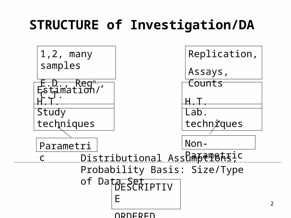
STRUCTURE of Investigation/DA

DESCRIPTIVE

ORDERED

Distributional Assumptions, Probability Basis: Size/Type of Data Set

Parametric Non-Parametric

Study techniques Lab. techniques

Estimation/H.T. H.T.

1,2, many samples

E.D., Regn., C.T.

Replication,

Assays, Counts

3

‘BIO’ CONTEXT here

• GENETICS : 5 branches; aim = ‘Laws’ of Chemistry, Physics, Maths. for Biology

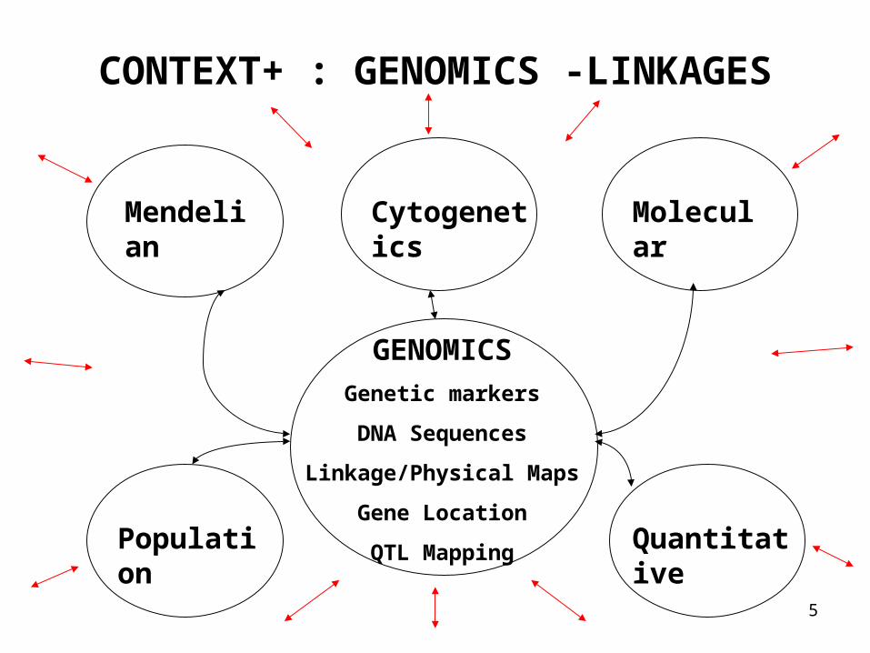
• GENOMICS : Study of Genomes (complete set of DNA carried by Gamete) by integration of 5 branches of Genetics with ‘Informatics and Automated systems’

• PURPOSE of GENOME RESEARCH : Info. on Structure, Function, Evolution of all Genomes – past and present

• Techniques of Genomics from molecular, quantitative, population genetics: Concepts and Terminology from Mendelian genetics and cytogenetics

4

CONTEXT: GENETICS - BRANCHES

• Classical Mendelian – Gene and Locus, Allele, Segregation, Gamete, Dominance, Mutation

• Cytogenetics – Cell, Chromasome, Meiosis and Mitosis, Crossover and Linkage

• Molecular – DNA sequencing, Gene Regulation and Transcription, Translation and Genetic Code Mutations

• Population – Allelic/Genotypic Frequencies, Equilibrium, Selection, Drift, Migration, Mutation

• Quantitative – Heritability/Additive, Non-additive Genetic Effects, Genetic by Environment Interaction, Plant and Animal Breeding

5

CONTEXT+ : GENOMICS -LINKAGES

Mendelian Cytogenetics Molecular

Population Quantitative

GENOMICS

Genetic markers

DNA Sequences

Linkage/Physical Maps

Gene Location

QTL Mapping

6

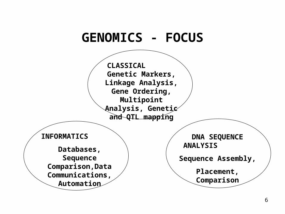
GENOMICS - FOCUS

CLASSICAL Genetic Markers,

Linkage Analysis, Gene Ordering, Multipoint Analysis, Genetic and

QTL mapping

INFORMATICS

Databases, Sequence Comparison,Data Communications,

Automation

DNA SEQUENCE ANALYSIS

Sequence Assembly,

Placement, Comparison

7

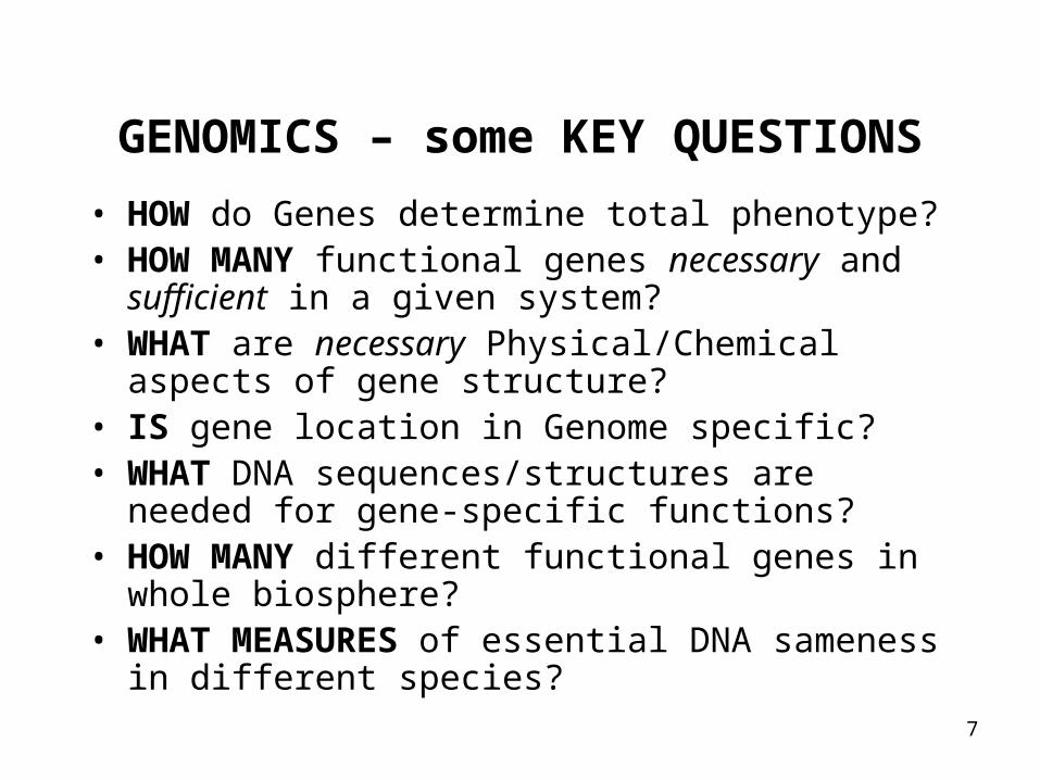
GENOMICS – some KEY QUESTIONS

• HOW do Genes determine total phenotype?• HOW MANY functional genes necessary and

sufficient in a given system?• WHAT are necessary Physical/Chemical aspects of

gene structure? • IS gene location in Genome specific?• WHAT DNA sequences/structures are needed for

gene-specific functions?• HOW MANY different functional genes in whole

biosphere?• WHAT MEASURES of essential DNA sameness in

different species?

8

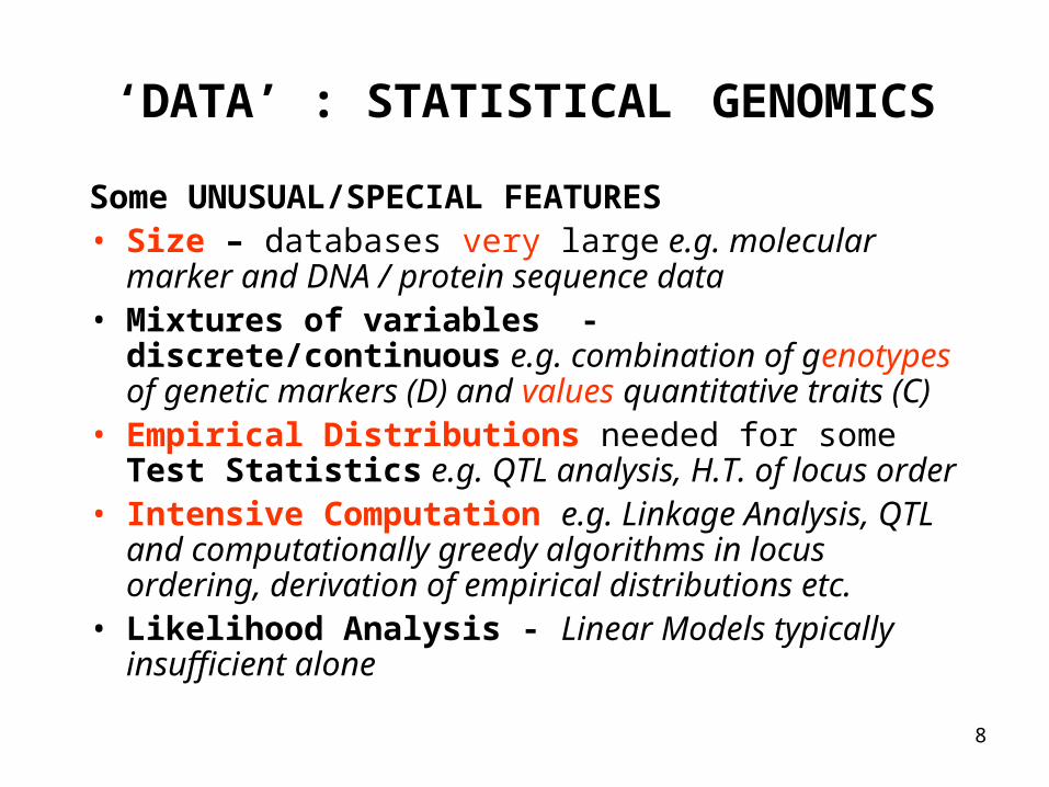
‘DATA’ : STATISTICAL GENOMICS

Some UNUSUAL/SPECIAL FEATURES• Size – databases very large e.g. molecular marker

and DNA / protein sequence data• Mixtures of variables - discrete/continuous e.g.

combination of genotypes of genetic markers (D) and values quantitative traits (C)

• Empirical Distributions needed for some Test Statistics e.g. QTL analysis, H.T. of locus order

• Intensive Computation e.g. Linkage Analysis, QTL and computationally greedy algorithms in locus ordering, derivation of empirical distributions etc.

• Likelihood Analysis - Linear Models typically insufficient alone

9

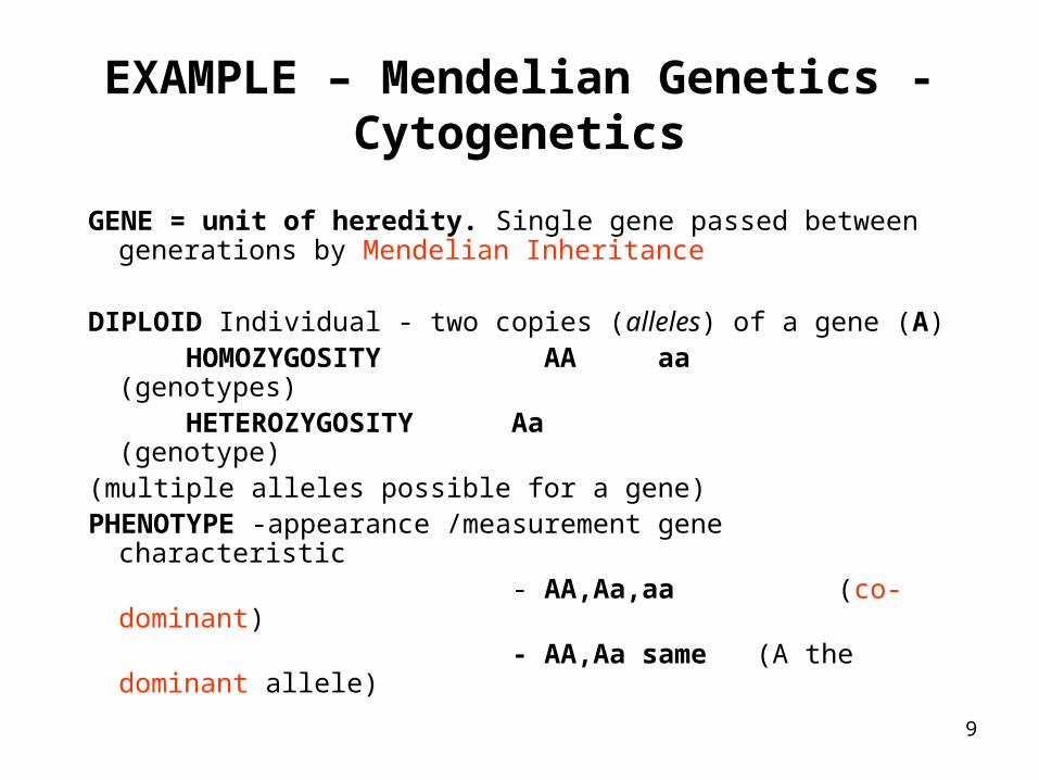
EXAMPLE – Mendelian Genetics - Cytogenetics

GENE = unit of heredity. Single gene passed between generations by Mendelian Inheritance

DIPLOID Individual - two copies (alleles) of a gene (A) HOMOZYGOSITY AA aa (genotypes) HETEROZYGOSITY Aa (genotype)(multiple alleles possible for a gene)PHENOTYPE -appearance /measurement gene

characteristic - AA,Aa,aa (co-dominant) - AA,Aa same (A the dominant allele)

10

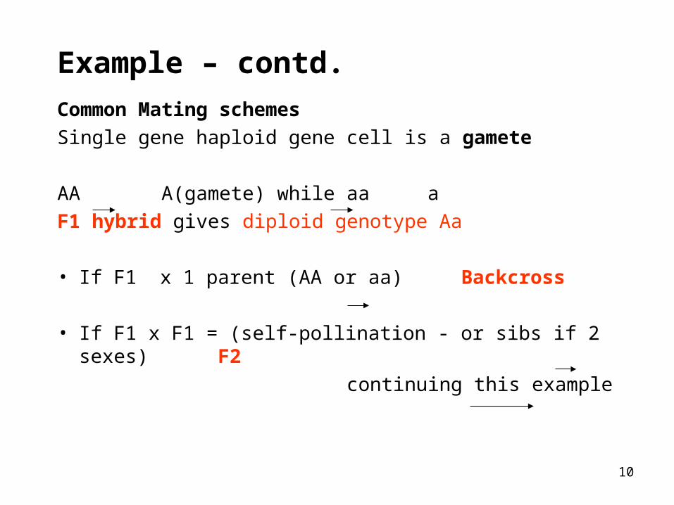
Example – contd.

Common Mating schemes

Single gene haploid gene cell is a gamete

AA A(gamete) while aa a

F1 hybrid gives diploid genotype Aa

• If F1 x 1 parent (AA or aa) Backcross

• If F1 x F1 = (self-pollination - or sibs if 2 sexes) F2

continuing this example

11

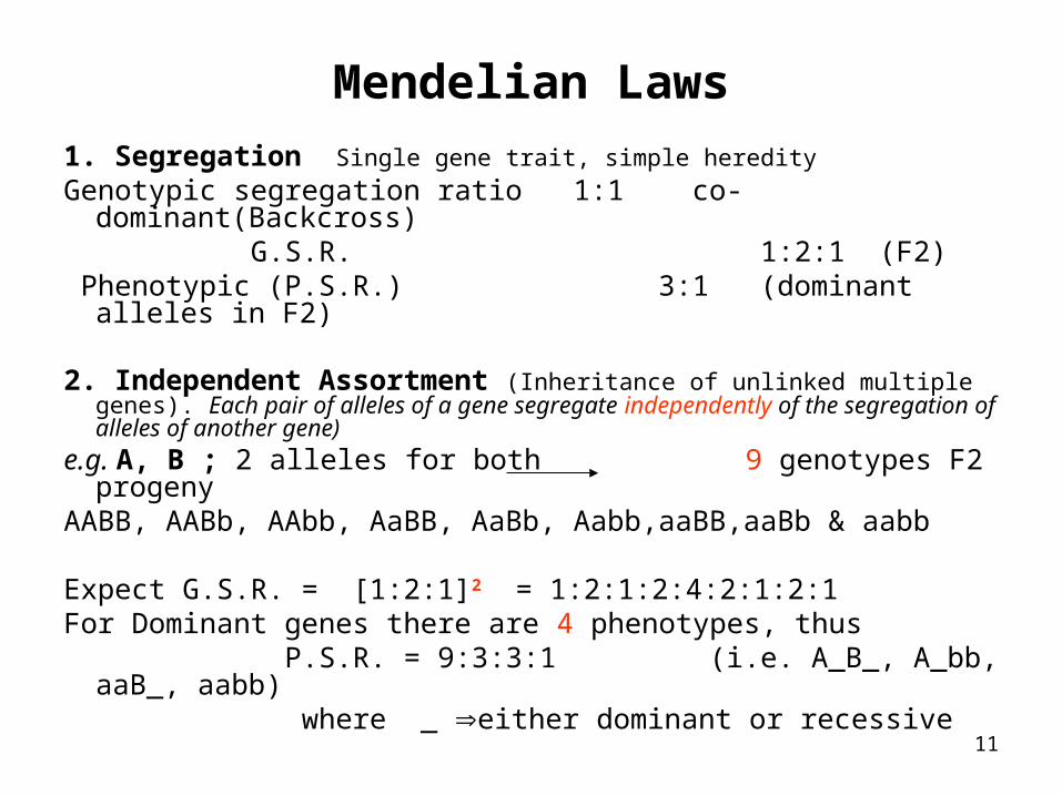
Mendelian Laws

1. Segregation Single gene trait, simple heredity

Genotypic segregation ratio 1:1 co-dominant(Backcross) G.S.R. 1:2:1 (F2) Phenotypic (P.S.R.) 3:1 (dominant alleles in F2)

2. Independent Assortment (Inheritance of unlinked multiple genes). Each pair of alleles of a gene segregate independently of the segregation of alleles of another gene)

e.g. A, B ; 2 alleles for both 9 genotypes F2 progenyAABB, AABb, AAbb, AaBB, AaBb, Aabb,aaBB,aaBb & aabb

Expect G.S.R. = [1:2:1]2 = 1:2:1:2:4:2:1:2:1For Dominant genes there are 4 phenotypes, thus P.S.R. = 9:3:3:1 (i.e. A_B_, A_bb, aaB_, aabb) where _ either dominant or recessive

12

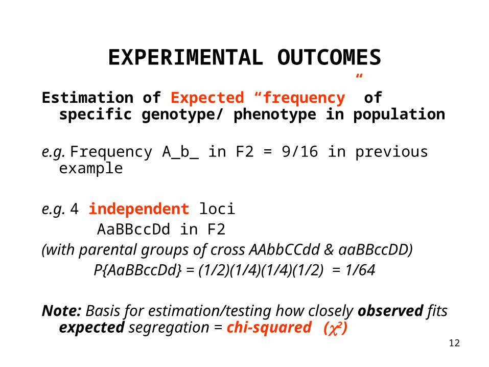
EXPERIMENTAL OUTCOMES

Estimation of Expected “frequency” of specific genotype/ phenotype in population

e.g. Frequency A_b_ in F2 = 9/16 in previous example

e.g. 4 independent loci AaBBccDd in F2 (with parental groups of cross AAbbCCdd & aaBBccDD) P{AaBBccDd} = (1/2)(1/4)(1/4)(1/2) = 1/64

Note: Basis for estimation/testing how closely observed fits expected segregation = chi-squared (2)

13

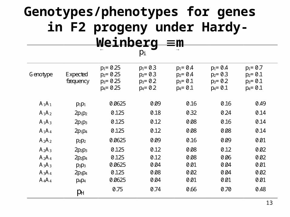
pi

Genotype Expectedfrequency

p1= 0.25p2= 0.25p3= 0.25p4= 0.25

p1= 0.3p2= 0.3p3= 0.2p4= 0.2

p1= 0.4p2= 0.4p3= 0.1p4= 0.1

p1= 0.4p2= 0.3p3= 0.2p4= 0.1

p1= 0.7p2= 0.1p3= 0.1p4= 0.1

A1A1 p1p1 0.0625 0.09 0.16 0.16 0.49

A1A2 2p1p2 0.125 0.18 0.32 0.24 0.14

A1A3 2p1p3 0.125 0.12 0.08 0.16 0.14

A1A4 2p1p4 0.125 0.12 0.08 0.08 0.14

A2A2 p2p2 0.0625 0.09 0.16 0.09 0.01

A2A3 2p2p3 0.125 0.12 0.08 0.12 0.02A2A4 2p2p4 0.125 0.12 0.08 0.06 0.02A3A3 p3p3 0.0625 0.04 0.01 0.04 0.01A3A4 2p3p4 0.125 0.08 0.02 0.04 0.02A4A4 p4p4 0.0625 0.04 0.01 0.01 0.01

pH0.75 0.74 0.66 0.70 0.48

Genotypes/phenotypes for genes in F2 progeny under Hardy-Weinberg m

14

Mechanisms of MENDELIAN HEREDITY:

• Cell division - mitosis, meiosis• Genetic Linkage = association of genes on same

chromasome Effects: Seg. Ratios no longer Mendelian. Result of

recombination (meiosis) is the existence of non-parental chromasomes in cellular meiotic products).

Each crossover (exchange of chromasomal segments between homologs) gives 2 reciprocal recombinant (non-parental) gametes. Measurement : recombinant fraction

• -Recombination generally random on chromasomes: recombination between loci associated with distance apart. (Basic premise - genetic/genomic mapping).

• Models: Linkage phase (co-dominance, experimental data), factors affecting recombination

15

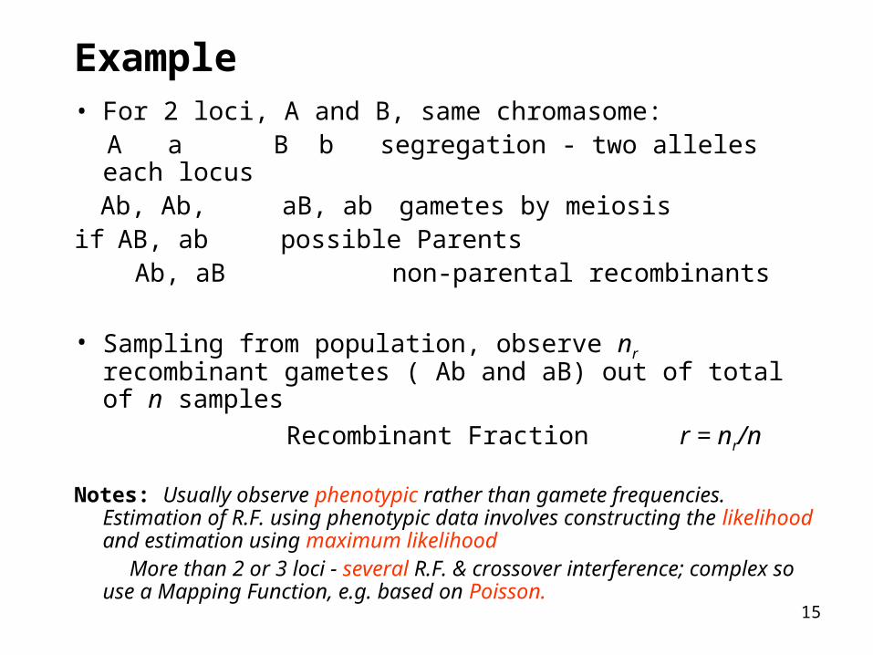
Example• For 2 loci, A and B, same chromasome: A a B b segregation - two alleles each locus Ab, Ab, aB, ab gametes by meiosisif AB, ab possible Parents Ab, aB non-parental recombinants

• Sampling from population, observe nr recombinant gametes ( Ab and aB) out of total of n samples

Recombinant Fraction r = nr/n

Notes: Usually observe phenotypic rather than gamete frequencies. Estimation of R.F. using phenotypic data involves constructing the likelihood and estimation using maximum likelihood

More than 2 or 3 loci - several R.F. & crossover interference; complex so use a Mapping Function, e.g. based on Poisson.

16

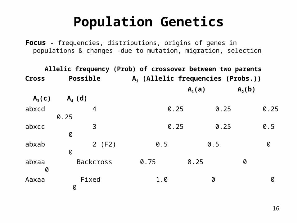
Population Genetics

Focus - frequencies, distributions, origins of genes in populations & changes -due to mutation, migration, selection

Allelic frequency (Prob) of crossover between two parents

Cross Possible Ai (Allelic frequencies (Probs.))

A1(a) A2(b) A3(c) A4 (d)

abxcd 4 0.25 0.25 0.25 0.25

abxcc 3 0.25 0.25 0.5 0

abxab 2 (F2) 0.5 0.5 0 0

abxaa Backcross 0.75 0.25 0 0

Aaxaa Fixed 1.0 0 0 0

17

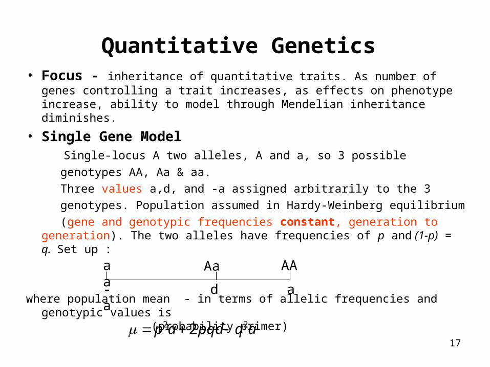
Quantitative Genetics • Focus - inheritance of quantitative traits. As number of genes

controlling a trait increases, as effects on phenotype increase, ability to model through Mendelian inheritance diminishes.

• Single Gene Model Single-locus A two alleles, A and a, so 3 possible

genotypes AA, Aa & aa.

Three values a,d, and -a assigned arbitrarily to the 3

genotypes. Population assumed in Hardy-Weinberg equilibrium

(gene and genotypic frequencies constant, generation to generation). The two alleles have frequencies of p and (1-p) = q. Set up :

where population mean - in terms of allelic frequencies and genotypic values is (probability primer)

-a d

AA

a

Aaaa

aqpqdap 22 2

18

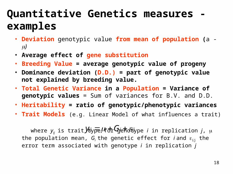
Quantitative Genetics measures - examples

• Deviation genotypic value from mean of population (a - )

• Average effect of gene substitution

• Breeding Value = average genotypic value of progeny

• Dominance deviation (D.D.) = part of genotypic value not explained by breeding value.

• Total Genetic Variance in a Population = Variance of genotypic values = Sum of variances for B.V. and D.D.

• Heritability = ratio of genotypic/phenotypic variances • Trait Models (e.g. Linear Model of what influences a trait)

where yij is trait type for genotype i in replication j, the population mean, Gi the genetic effect for i and ij the error term associated with genotype i in replication j

ijiij Gy

Probability & Statistics Primer -appendix, if needed

Note: Short overview. Other statistical distributions in lectures

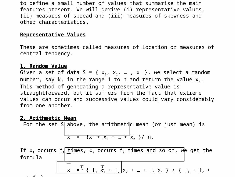
Summary Statistics- DescriptiveWhen analysing practical sets of data, it is useful to be able to define a small number of values that summarise the main features present. We will derive (i) representative values, (ii) measures of spread and (iii) measures of skewness and other characteristics.

Representative Values

These are sometimes called measures of location or measures of central tendency.

1. Random ValueGiven a set of data S = { x1, x2, … , xn }, we select a random number, say k, in the range 1 to n and return the value xk. This method of generating a representative value is straightforward, but it suffers from the fact that extreme values can occur and successive values could vary considerably from one another.

2. Arithmetic Mean For the set S above, the arithmetic mean (or just mean) is

x = {x1 + x2 + … + xn }/ n.

If x1 occurs f1 times, x2 occurs f2 times and so on, we get the formula

x = { f1 x1 + f2 x2 + … + fn xn } / { f1 + f2 + … + fn } ,

written x = f x / f

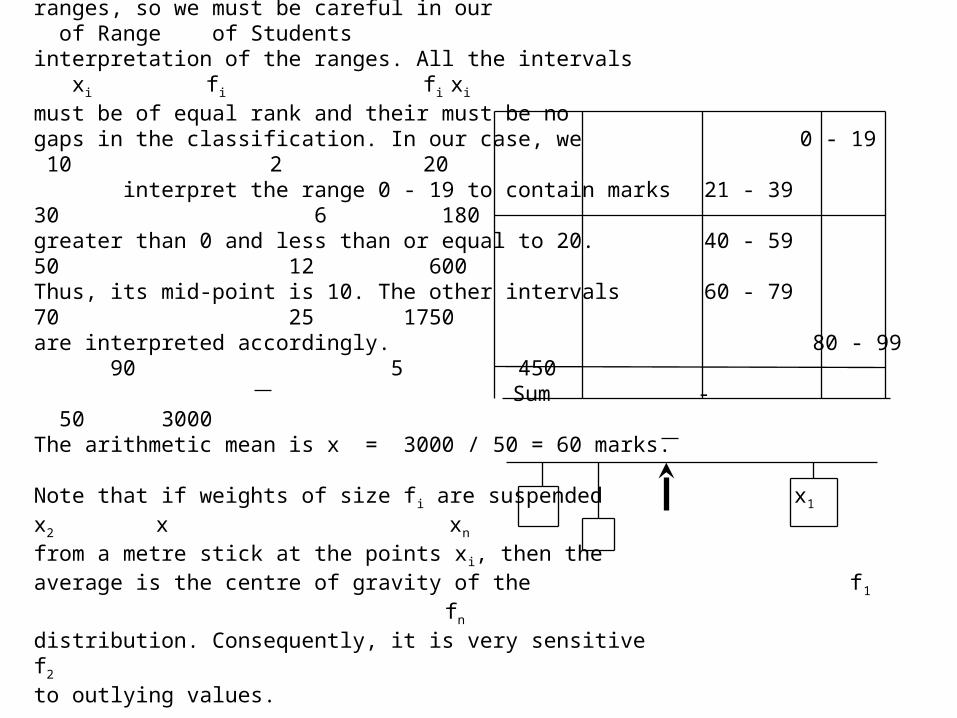
Example 1. The data refers to the marks that students in a class obtained in an examination. Find the average mark for the class. The firstpoint to note is that the marks are presented as Mark Mid-Point Numberranges, so we must be careful in our of Range of Studentsinterpretation of the ranges. All the intervals x i fi fi xi must be of equal rank and their must be no gaps in the classification. In our case, we 0 - 19 10 2 20 interpret the range 0 - 19 to contain marks 21 - 39 30 6 180greater than 0 and less than or equal to 20. 40 - 59 50 12 600Thus, its mid-point is 10. The other intervals 60 - 79 70 25 1750 are interpreted accordingly. 80 - 99 90 5 450 Sum - 50 3000 The arithmetic mean is x = 3000 / 50 = 60 marks.

Note that if weights of size fi are suspended x1 x2 x xn

from a metre stick at the points xi, then the average is the centre of gravity of the f1 fn

distribution. Consequently, it is very sensitive f2

to outlying values.

Equally, the population should be homogenous for the average to be meaningful. For example, if we assume that the typical height of girls in a class is less than that of boys, then the average height of all students is neither representative of the girls or the boys.

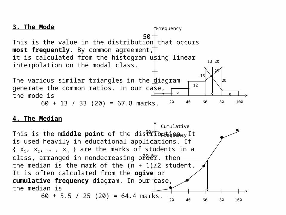
3. The Mode

This is the value in the distribution that occurs most frequently. By common agreement,it is calculated from the histogram using linear interpolation on the modal class.

The various similar triangles in the diagram generate the common ratios. In our case, the mode is

60 + 13 / 33 (20) = 67.8 marks.

4. The Median

This is the middle point of the distribution. It is used heavily in educational applications. If{ x1, x2, … , xn } are the marks of students in a class, arranged in nondecreasing order, then the median is the mark of the (n + 1)/2 student.It is often calculated from the ogive or cumulative frequency diagram. In our case,the median is

60 + 5.5 / 25 (20) = 64.4 marks.

50Frequency

20

20 40 60 80 100

6

12

25

52

13

13

20

Cumulative

Frequency

10080604020

50

25.5

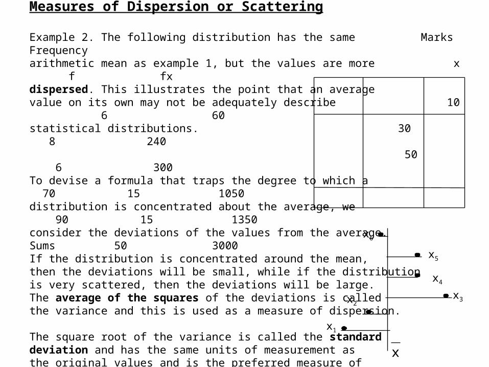
Measures of Dispersion or Scattering

Example 2. The following distribution has the same Marks Frequencyarithmetic mean as example 1, but the values are more x f fxdispersed. This illustrates the point that an average value on its own may not be adequately describe 10 6 60statistical distributions. 30 8 240

50 6 300To devise a formula that traps the degree to which a 70 15 1050distribution is concentrated about the average, we 90 15 1350consider the deviations of the values from the average. Sums 50 3000If the distribution is concentrated around the mean, then the deviations will be small, while if the distribution is very scattered, then the deviations will be large. The average of the squares of the deviations is called the variance and this is used as a measure of dispersion.

The square root of the variance is called the standard deviation and has the same units of measurement as the original values and is the preferred measure of dispersion in many applications. x1

x2x3

x4

x5

x6

x

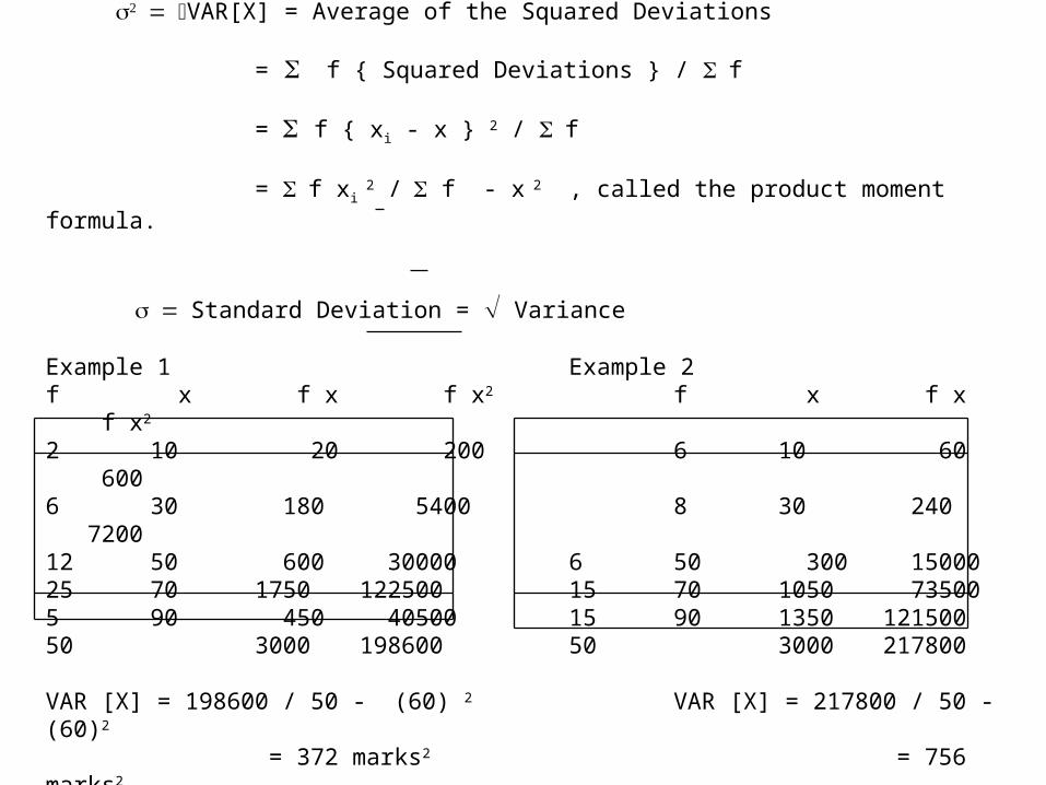
Variance & Standard Deviation

VAR[X] = Average of the Squared Deviations

= f { Squared Deviations } / f

= f { xi - x } 2 / f

= f xi 2 / f - x 2 , called the product moment formula.

Standard Deviation = Variance

Example 1 Example 2f x f x f x2 f x f x f x2

2 10 20 200 6 10 60 6006 30 180 5400 8 30 240 720012 50 600 30000 6 50 300 1500025 70 1750 122500 15 70 1050 735005 90 450 40500 15 90 1350 12150050 3000 198600 50 3000 217800

VAR [X] = 198600 / 50 - (60) 2 VAR [X] = 217800 / 50 - (60)2

= 372 marks2 = 756 marks2

Other Summary Statistics

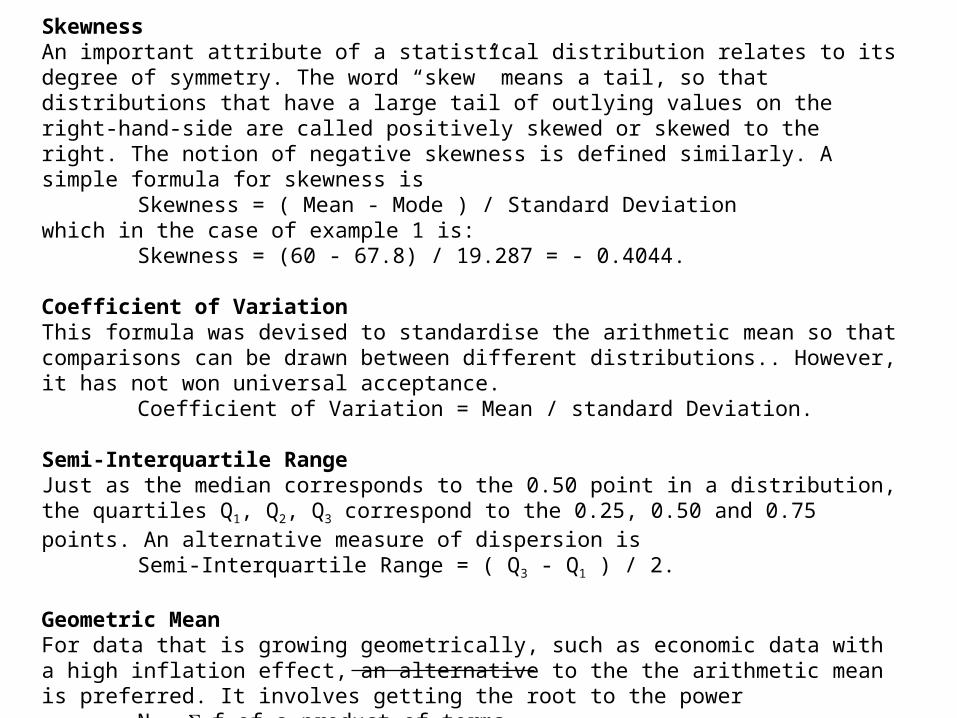
SkewnessAn important attribute of a statistical distribution relates to its degree of symmetry. The word “skew” means a tail, so that distributions that have a large tail of outlying values on the right-hand-side are called positively skewed or skewed to the right. The notion of negative skewness is defined similarly. A simple formula for skewness is

Skewness = ( Mean - Mode ) / Standard Deviationwhich in the case of example 1 is:

Skewness = (60 - 67.8) / 19.287 = - 0.4044.

Coefficient of VariationThis formula was devised to standardise the arithmetic mean so that comparisons can be drawn between different distributions.. However, it has not won universal acceptance.

Coefficient of Variation = Mean / standard Deviation.

Semi-Interquartile RangeJust as the median corresponds to the 0.50 point in a distribution, the quartiles Q1, Q2, Q3 correspond to the 0.25, 0.50 and 0.75 points. An alternative measure of dispersion is

Semi-Interquartile Range = ( Q3 - Q1 ) / 2.

Geometric MeanFor data that is growing geometrically, such as economic data with a high inflation effect, an alternative to the the arithmetic mean is preferred. It involves getting the root to the power

N = f of a product of terms

Geometric Mean = Nx1f1 x2 f2 … xk fk

Regression

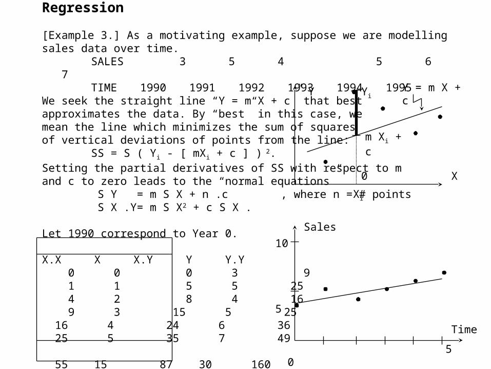
[Example 3.] As a motivating example, suppose we are modelling sales data over time.SALES 3 5 4 5 6 7TIME 1990 1991 1992 1993 1994 1995

We seek the straight line “Y = m X + c” that best approximates the data. By “best” in this case, we mean the line which minimizes the sum of squaresof vertical deviations of points from the line:

SS = S ( Yi - [ mXi + c ] ) 2.

Setting the partial derivatives of SS with respect to m and c to zero leads to the “normal equations”

S Y = m S X + n .c , where n = # points S X .Y= m S X2 + c S X .

Let 1990 correspond to Year 0.

X.X X X.Y Y Y.Y 0 0 0 3 9 1 1 5 5 25 4 2 8 4 16 9 3 15 5 25 16 4 24 6 36 25 5 35 7 49

55 15 87 30 160

X

Y Y = m X + c

m Xi + c

Yi

0

Xi

Time

Sales

10

5

0 5

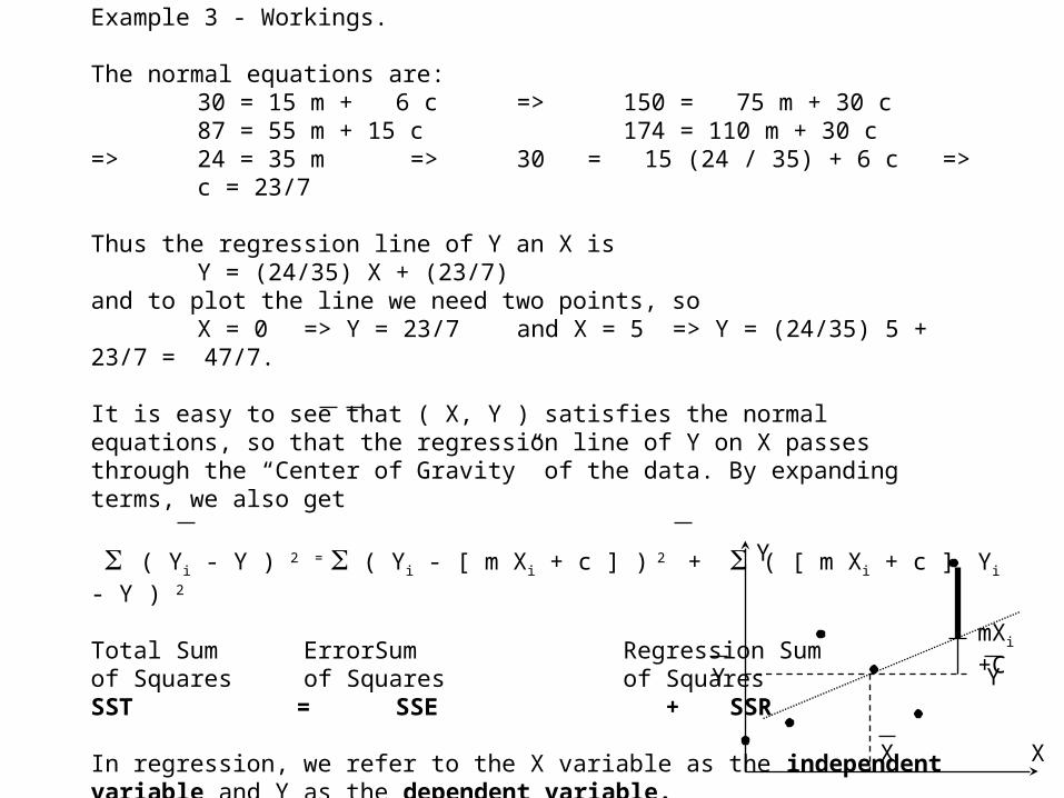
Example 3 - Workings.

The normal equations are:30 = 15 m + 6 c => 150 = 75 m + 30 c 87 = 55 m + 15 c 174 = 110 m + 30 c

=> 24 = 35 m=> 30 = 15 (24 / 35) + 6 c => c = 23/7

Thus the regression line of Y an X isY = (24/35) X + (23/7)

and to plot the line we need two points, soX = 0 => Y = 23/7 and X = 5 => Y = (24/35) 5 + 23/7 = 47/7.

It is easy to see that ( X, Y ) satisfies the normal equations, so that the regression line of Y on X passes through the “Center of Gravity” of the data. By expanding terms, we also get

( Yi - Y ) 2 = ( Yi - [ m Xi + c ] ) 2 + ( [ m Xi + c ] - Y ) 2

Total Sum ErrorSum Regression Sumof Squares of Squares of SquaresSST = SSE + SSR

In regression, we refer to the X variable as the independentvariable and Y as the dependent variable.

X

Y

Yi

mXi +C

Y

X

Y

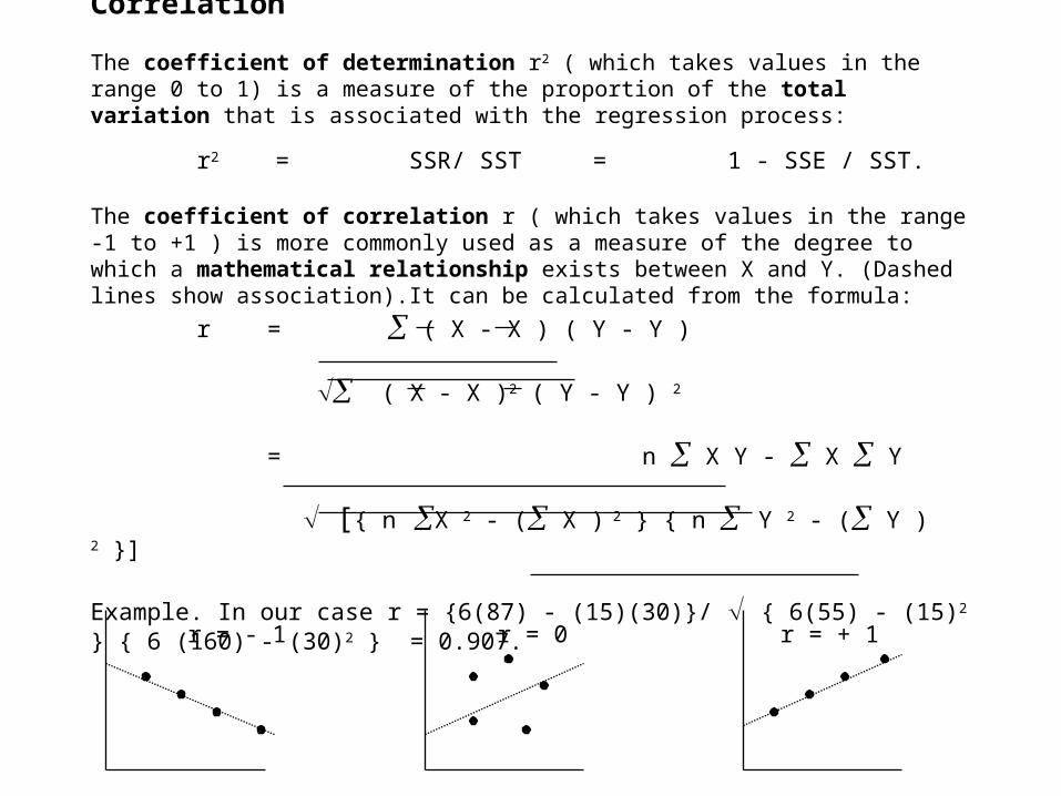
Correlation

The coefficient of determination r2 ( which takes values in the range 0 to 1) is a measure of the proportion of the total variation that is associated with the regression process:

r2 = SSR/ SST = 1 - SSE / SST.

The coefficient of correlation r ( which takes values in the range -1 to +1 ) is more commonly used as a measure of the degree to which a mathematical relationship exists between X and Y. (Dashed lines show association).It can be calculated from the formula:

r = ( X - X ) ( Y - Y )

( X - X )2 ( Y - Y ) 2

= n X Y - X Y

[{ n X 2 - ( X ) 2 } { n Y 2 - ( Y ) 2 }]

Example. In our case r = {6(87) - (15)(30)}/ { 6(55) - (15)2 } { 6 (160) - (30)2 } = 0.907.

r = - 1 r = + 1r = 0

Collinearity

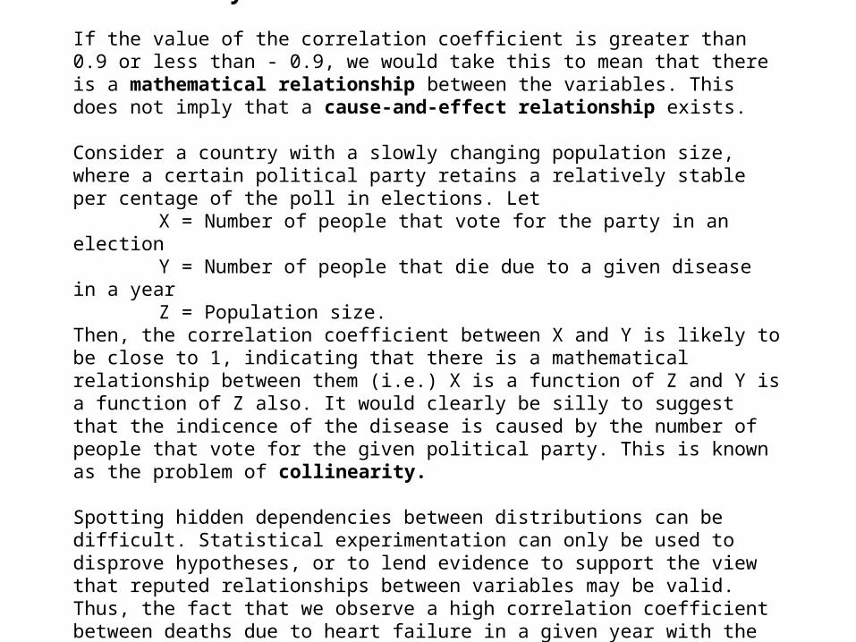
If the value of the correlation coefficient is greater than 0.9 or less than - 0.9, we would take this to mean that there is a mathematical relationship between the variables. This does not imply that a cause-and-effect relationship exists.

Consider a country with a slowly changing population size, where a certain political party retains a relatively stable per centage of the poll in elections. Let

X = Number of people that vote for the party in an electionY = Number of people that die due to a given disease in a yearZ = Population size.

Then, the correlation coefficient between X and Y is likely to be close to 1, indicating that there is a mathematical relationship between them (i.e.) X is a function of Z and Y is a function of Z also. It would clearly be silly to suggest that the indicence of the disease is caused by the number of people that vote for the given political party. This is known as the problem of collinearity.

Spotting hidden dependencies between distributions can be difficult. Statistical experimentation can only be used to disprove hypotheses, or to lend evidence to support the view that reputed relationships between variables may be valid. Thus, the fact that we observe a high correlation coefficient between deaths due to heart failure in a given year with the number of cigarettes consumed twenty years earlier does not establish a cause-and-effect relationship. However, this result may be of value in directing biological research.

Overview of Probability Theory

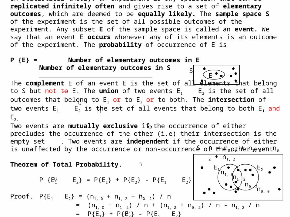
In statistical theory, an experiment is any operation that can be replicated infinitely often and gives rise to a set of elementary outcomes, which are deemed to be equally likely. The sample space S of the experiment is the set of all possible outcomes of the experiment. Any subset E of the sample space is called an event. We say that an event E occurs whenever any of its elements is an outcome of the experiment. The probability of occurrence of E is

P {E} = Number of elementary outcomes in ENumber of elementary outcomes in S

The complement E of an event E is the set of all elements that belong to S but not to E. The union of two events E1 E2 is the set of all outcomes that belong to E1 or to E2 or to both. The intersection of two events E1 E2 is the set of all events that belong to both E1 and E2.

Two events are mutually exclusive if the occurrence of either precludes the occurrence of the other (i.e) their intersection is the empty set . Two events are independent if the occurrence of either is unaffected by the occurrence or non-occurrence of the other event.

Theorem of Total Probability.

P {E1 E2} = P{E1} + P{E2} - P{E1 E2}

Proof. P{E1 E2} = (n1, 0 + n1, 2 + n0, 2) / n = (n1, 0 + n1, 2) / n + (n1, 2 + n0, 2) / n - n1, 2 / n = P{E1} + P{E2} - P{E1 E2}

Corollary.If E1 and E2 are mutually exclusive, P{E1 E2} = P{E1} + P{E2} - see Axioms and Addition Rule

ES

n = n0, 0 + n1, 0 + n0, 2 + n1, 2

E1 E2

S

n1, 0 n1, 2

n0, 2 n0, 0

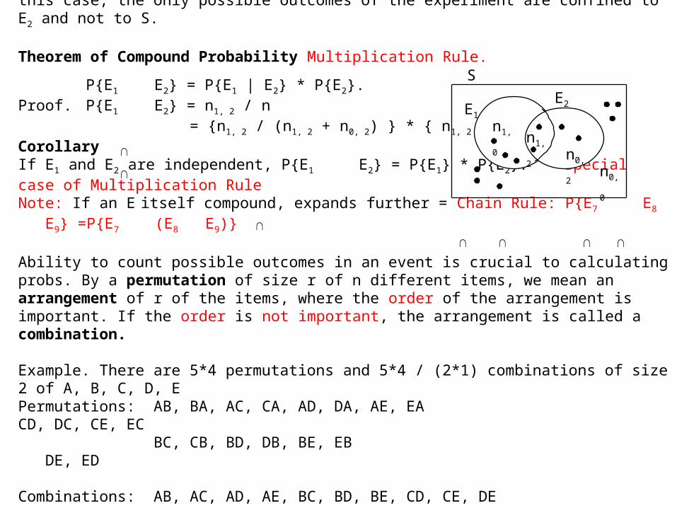
The probability P{E1 | E2} that E1 occurs, given that E2 has occurred (or must occur) is called the conditional probability of E1. Note that in this case, the only possible outcomes of the experiment are confined to E2 and not to S. Theorem of Compound Probability Multiplication Rule.

P{E1 E2} = P{E1 | E2} * P{E2}. Proof. P{E1 E2} = n1, 2 / n

= {n1, 2 / (n1, 2 + n0, 2) } * { n1, 2 + n0, 2) / n}CorollaryIf E1 and E2 are independent, P{E1 E2} = P{E1} * P{E2}. Special case of Multiplication RuleNote: If an E itself compound, expands further = Chain Rule: P{E7 E8 E9} =P{E7 (E8 E9)}

Ability to count possible outcomes in an event is crucial to calculating probs. By a permutation of size r of n different items, we mean an arrangement of r of the items, where the order of the arrangement is important. If the order is not important, the arrangement is called a combination.

Example. There are 5*4 permutations and 5*4 / (2*1) combinations of size 2 of A, B, C, D, EPermutations: AB, BA, AC, CA, AD, DA, AE, EA CD, DC, CE, EC

BC, CB, BD, DB, BE, EB DE, ED

Combinations: AB, AC, AD, AE, BC, BD, BE, CD, CE, DE

Standard reference books on probability theory give a comprehensive treatment of how these ideas are used to calculate the probability of occurrence of the outcomes of games of chance.

n1, 0 n1, 2

n0, 2

n0, 0

E1

E2

S

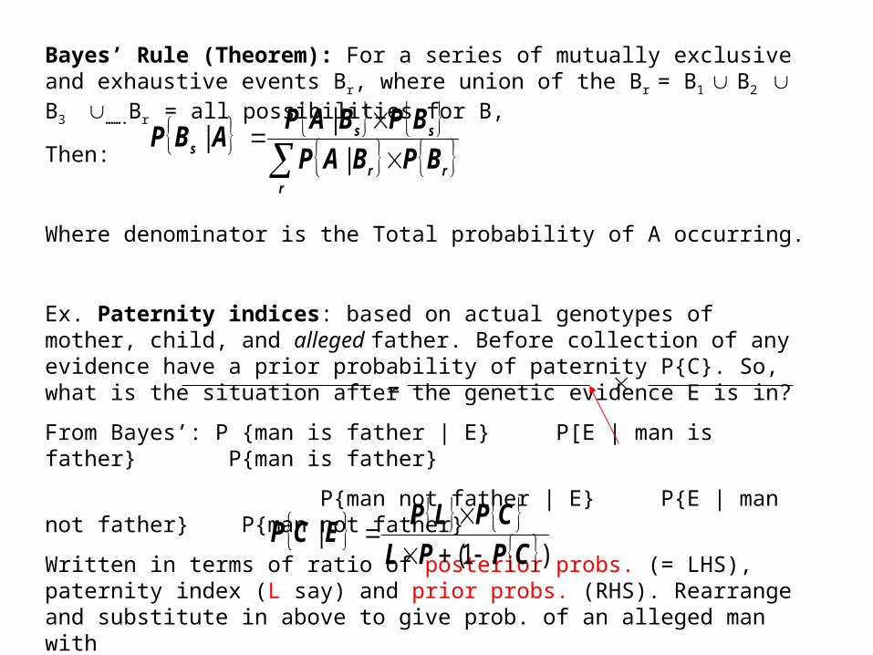
Bayes’ Rule (Theorem): For a series of mutually exclusive and exhaustive events Br, where union of the Br = B1 B2 B3 …….Br = all possibilities for B,

Then:

Where denominator is the Total probability of A occurring.

Ex. Paternity indices: based on actual genotypes of mother, child, and alleged father. Before collection of any evidence have a prior probability of paternity P{C}. So, what is the situation after the genetic evidence E is in?

From Bayes’: P {man is father | E} P[E | man is father} P{man is father}

P{man not father | E} P{E | man not father} P{man not father}

Written in terms of ratio of posterior probs. (= LHS), paternity index (L say) and prior probs. (RHS). Rearrange and substitute in above to give prob. of an alleged man with

particular genotype

being the true father

NB: L is a way of ‘weighting’ the genetic evidence; the issue is setting a prior.

rrr

sss BPBAP

BPBAPABP

|

||

=

)1(

|CPPL

CPLPECP

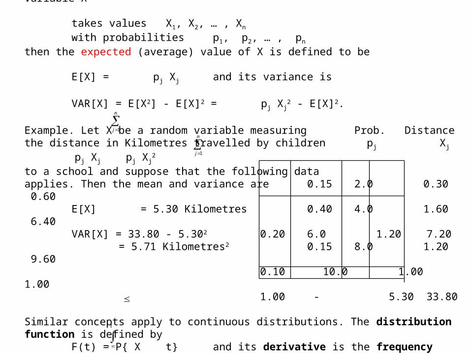
Statistical Distributions- CharacterisationIf a statistical experiment only gives rise to real numbers, the outcome of the experiment is called a random variable. If a random variable X

takes values X1, X2, … , Xn

with probabilities p1, p2, … , pn

then the expected (average) value of X is defined to be

E[X] = pj Xj and its variance is

VAR[X] = E[X2] - E[X]2 = pj Xj2 - E[X]2.

Example. Let X be a random variable measuring Prob. Distancethe distance in Kilometres travelled by children pj Xj pj Xj pj Xj

2

to a school and suppose that the following data applies. Then the mean and variance are 0.15 2.0 0.30 0.60

E[X] = 5.30 Kilometres 0.40 4.0 1.60 6.40VAR[X] = 33.80 - 5.302 0.20 6.0 1.20 7.20

= 5.71 Kilometres2 0.15 8.0 1.20 9.600.10 10.0 1.00 1.001.00 - 5.30 33.80

Similar concepts apply to continuous distributions. The distribution function is defined byF(t) = P{ X t} and its derivative is the frequency functionf(t) = d F(t) / dt

so that F(t) = f(x) dx.

j

n

1

j

n

1

t

Sums and Differences of Random Variables

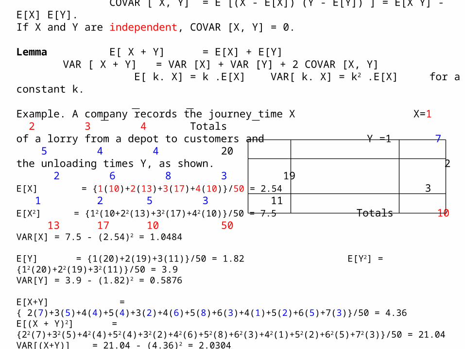
Define the covariance of two random variables to be COVAR [ X, Y] = E [(X - E[X]) (Y - E[Y]) ] = E[X Y] - E[X] E[Y].

If X and Y are independent, COVAR [X, Y] = 0.

Lemma E[ X + Y] = E[X] + E[Y]VAR [ X + Y] = VAR [X] + VAR [Y] + 2 COVAR [X, Y]

E[ k. X] = k .E[X] VAR[ k. X] = k2 .E[X] for a constant k.

Example. A company records the journey time X X=1 2 3 4 Totalsof a lorry from a depot to customers and Y =1 7 5 4 4 20 the unloading times Y, as shown. 2 2 6 8 3 19E[X] = {1(10)+2(13)+3(17)+4(10)}/50 = 2.54 3 1 2 5 3 11E[X2] = {12(10+22(13)+32(17)+42(10)}/50 = 7.5 Totals 10 13 17 10 50 VAR[X] = 7.5 - (2.54)2 = 1.0484

E[Y] = {1(20)+2(19)+3(11)}/50 = 1.82 E[Y2] = {12(20)+22(19)+32(11)}/50 = 3.9VAR[Y] = 3.9 - (1.82)2 = 0.5876

E[X+Y] = { 2(7)+3(5)+4(4)+5(4)+3(2)+4(6)+5(8)+6(3)+4(1)+5(2)+6(5)+7(3)}/50 = 4.36 E[(X + Y)2] = {22(7)+32(5)+42(4)+52(4)+32(2)+42(6)+52(8)+62(3)+42(1)+52(2)+62(5)+72(3)}/50 = 21.04VAR[(X+Y)] = 21.04 - (4.36)2 = 2.0304

E[X Y] = {1(7)+2(5)+3(4)+4(4)+2(2)+4(6)+6(8)+8(3)+3(1)+6(2)+9(5)+12(3)}/50 = 4.82COVAR (X, Y) = 4.82 - (2.54)(1.82) = 0.1972VAR[X] + VAR[Y] + 2 COVAR[ X, Y] = 1.0484 + 0.5876 + 2 ( 0.1972) = 2.0304

Standard Statistical Distributions

Most elementary statistical books provide a survey of commonly used statistical distributions.

Importantly, we can characterise them by their expectation and variance (as for random variables) and by the parameters on which these are based; (see lecture notes for those we will refer to).

So, e.g. for a Binomial distribution, the parameters are p the probability of success in an individual trial and n the No. of trials.The probability of success remains constant – otherwise, another distribution applies.

Use of the correct distribution is core to statistical inference – I.e. estimating what is happening in the population on the basis of a (correctly drawn, probabilistic) sample.The sample is then representative of the population.

Fundamental to statistical inference is the Normal (or Gaussian), with parameters, the mean (or more formally expectation of the distribution) and (or 2), the Standard deviation ( Variance). For small samples, or when 2 not known but must be estimated from the sample, a slightly more conservative distribution applies = the Student’s T or just ‘t’ distribution. Introduces the degrees of freedom concept.

Student’s t Distribution

A random variable X has a t distribution with n degrees of freedom ( tn ) .

The t distribution is symmetrical about the origin, withE[X] = 0VAR [X] = n / (n -2).

For small values of n, the tn distribution is very flat. As n is increased the density assumes a bell shape. For values of n 25, the tn distribution is practically indistinguishable from the standard normal curve.

O If X and Y are independent random variables If X has a standard normal distribution and Y has a n

2 distribution then X has a tn distribution (Y / n)

O If x1, x2, … , xn is a random sample from a normal distribution, with mean and variance and if we define s2 = 1 / ( n - 1) ( xi - x ) 2

then ( x - ) / ( s / n) has a tn- 1 distribution

Estimated Sample variance see W,Y and S tables

+ Many other standard distributions

Sampling Theory

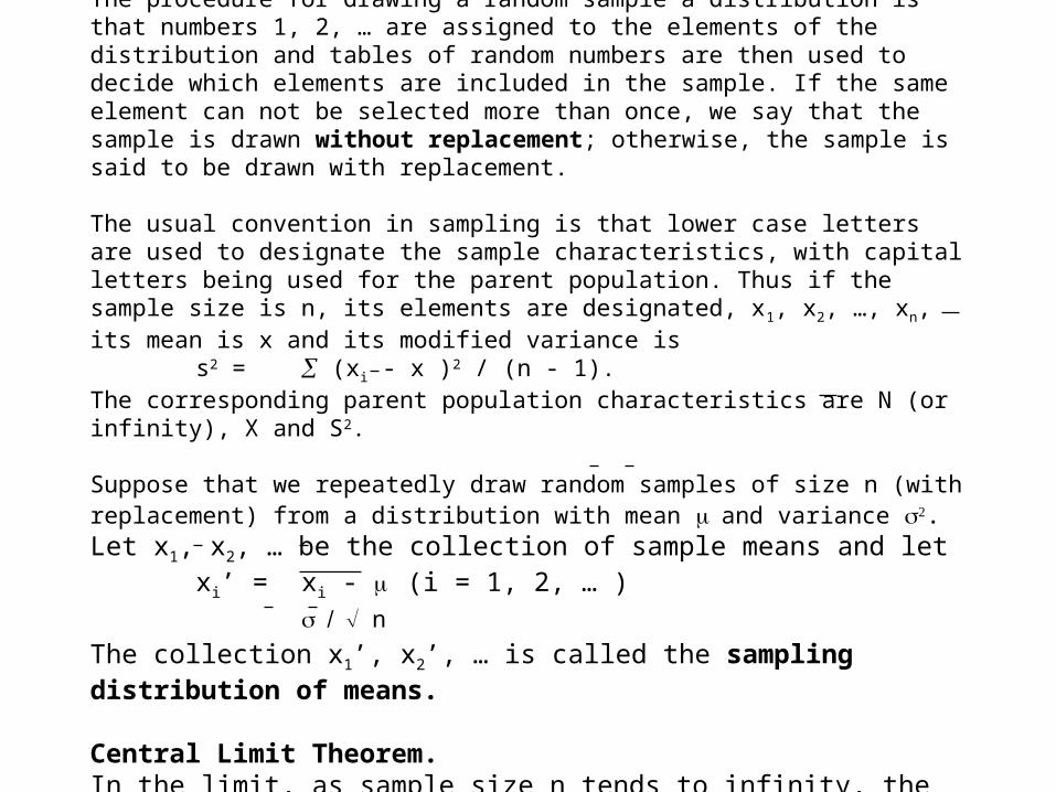
The procedure for drawing a random sample a distribution is that numbers 1, 2, … are assigned to the elements of the distribution and tables of random numbers are then used to decide which elements are included in the sample. If the same element can not be selected more than once, we say that the sample is drawn without replacement; otherwise, the sample is said to be drawn with replacement.

The usual convention in sampling is that lower case letters are used to designate the sample characteristics, with capital letters being used for the parent population. Thus if the sample size is n, its elements are designated, x1, x2, …, xn, its mean is x and its modified variance is

s2 = (xi - x )2 / (n - 1).The corresponding parent population characteristics are N (or infinity), X and S2.

Suppose that we repeatedly draw random samples of size n (with replacement) from a distribution with mean and variance . Let x1, x2, … be the collection of sample means and let

xi’ = xi - (i = 1, 2, … ) n

The collection x1’, x2’, … is called the sampling distribution of means.

Central Limit Theorem.In the limit, as sample size n tends to infinity, the sampling distribution of means has a standard normal distribution. Basis for statistical inference.

Attribute and Proportionate Sampling

If the sample elements area measurement of some characteristic, we are said to have attribute sampling. On the other hand if all the sample elements are 1 or 0 (success/failure, agree/ no-not-agree), we have proportionate sampling. For proportionate sampling, the sample average x and the sample proportion p are synonymous, just as are the mean and proportion P for the parent population. From our results on the Binomial distribution, the sample variance is p (1 - p) and the variance of the parent distribution is P (1 - P).

We can generalise the concept of the sampling distribution of means to get the sampling distribution of any statistic. We say that a sample characteristic is an unbiased estimator of the parent population characteristic, i.e. the expectation of the corresponding sampling distribution is equal to the parent characteristic.

Lemma. The sample average (proportion ) is an unbiased estimator of the parent average (proportion):

E [ x] = so E [p] = P.

The quantity ( N - n) / ( N - 1) is called the finite population correction (fpc). If the parent population is infinite or we have sampling with replacement the fpc = 1.

Lemma. E [s] = S * fpc for estimated sample S.D. with fpc

Confidence Intervals

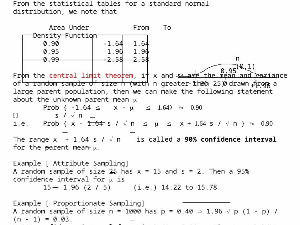
From the statistical tables for a standard normal distribution, we note that

Area Under From To Density Function

0.90 -1.64 1.640.95 -1.96 1.960.99 -2.58 2.58

From the central limit theorem, if x and s2 are the mean and variance of a random sample of size n (with n greater than 25) drawn from a large parent population, then we can make the following statement about the unknown parent mean

Prob { -1.64 x - s / ni.e. Prob { x - 1.64 s / n xs / n }

The range x + 1.64 s / n is called a 90% confidence interval for the parent mean . Example [ Attribute Sampling]A random sample of size 25 has x = 15 and s = 2. Then a 95% confidence interval for is

15 + 1.96 (2 / 5) (i.e.) 14.22 to 15.78

Example [ Proportionate Sampling]A random sample of size n = 1000 has p = 0.40 1.96 p (1 - p) / (n - 1) = 0.03.A 95% confidence interval for P is 0.40 + 0.03 (i.e.) 0.37 to 0.43.

n (0,1)

0-1.96 +1.96

0.95

Small Sampling Theory

For reference purposes, it is useful to regard the expression x + 1.96 s / n

as the “default formula” for a confidence interval and to modify it to suit particular circumstances.

O If we are dealing with proportionate sampling, the sample proportion is the sample mean and the standard error (s.e.) term s / n simplifies as follows: x -> p and s / n -> p(1 - p) / (n -1). (Also n-1 -> n) O A 90% confidence interval will bring about the swap 1.96 -> 1.64. O If the sample size n is less than 25, the normal distribution must be replaced by Student’s t n - 1 distribution. O For sampling without replacement from a finite population, a fpc term must be used.

The width of the confidence interval band increases with the confidence level.

Example. A random sample of size n = 10, drawn from a large parent population, has a mean x = 12 and a standard deviation s = 2. Then a 99% confidence interval for the parent mean is

x + 3.25 s / n (i.e.) 12 + 3.25 (2)/3 (i.e.) 9.83 to 14.17and a 95% confidence interval for the parent mean is

x + 2.262 s / n (i.e.) 12 + 2.262 (2)/3 (i.e.) 10.492 to 13.508.

Note that for n = 1000, 1.96 p (1 - p) / n for values of pbetween 0.3 and 0.7. This gives rise to the statement that public opinion polls have an “inherent error of 3%”. This simplifies calculations in the case of public opinion polls for large political parties.

Tests of Hypothesis

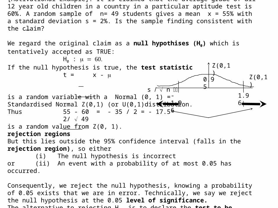
[Motivational Example]. It is claimed that the average grade of all 12 year old children in a country in a particular aptitude test is 60%. A random sample of n= 49 students gives a mean x = 55% with a standard deviation s = 2%. Is the sample finding consistent with the claim?

We regard the original claim as a null hypothises (H0) which is tentatively accepted as TRUE:

H0 : If the null hypothesis is true, the test statistic

t = x -

s nis a random variable with a Normal (0, 1) = Standardised Normal Z(0,1) (or U(0,1)distribution.Thus 55 - 60 = - 35 / 2 = - 17.5

2/ 49 is a random value from Z(0, 1). rejection regions But this lies outside the 95% confidence interval (falls in the rejection region), so either

(i) The null hypothesis is incorrector (ii) An event with a probability of at most 0.05 has occurred.

Consequently, we reject the null hypothesis, knowing a probability of 0.05 exists that we are in error. Technically, we say we reject the null hypothesis at the 0.05 level of significance.The alternative to rejecting H0, is to declare the test to be inconclusive. This means that there is some tentative evidence to support the view that H0 is approximately correct.

Z(0,1)0.95

1.96-1.96

Z(0,1)

Modifications

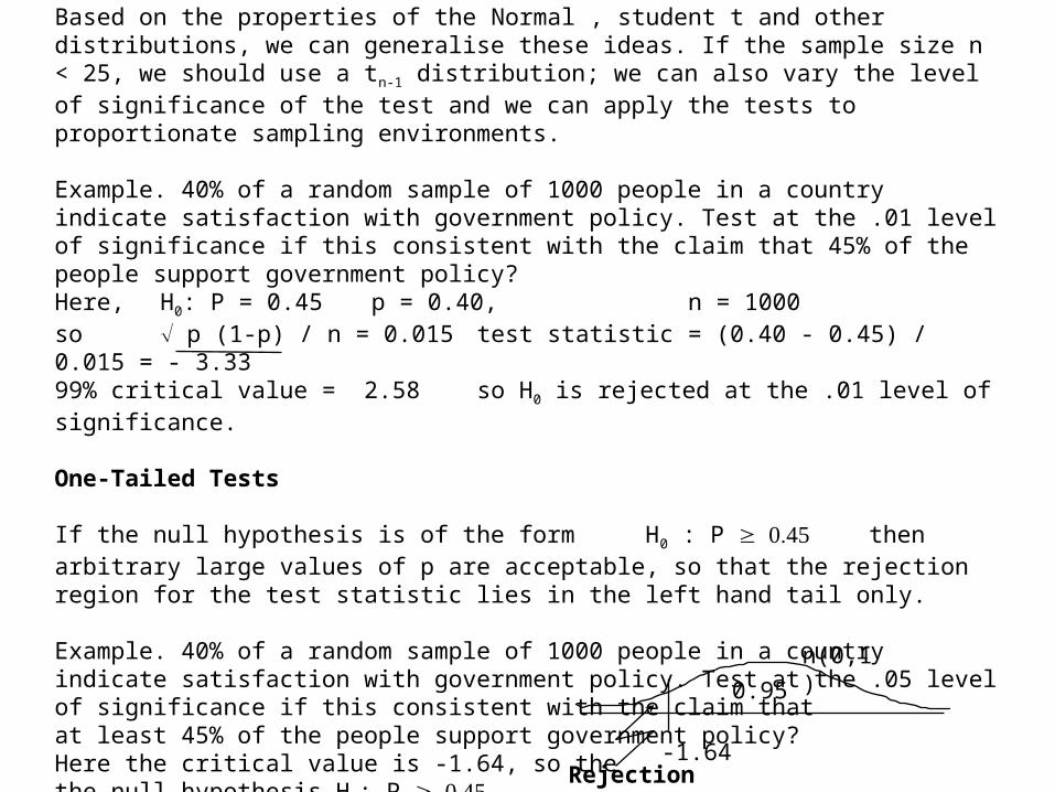
Based on the properties of the Normal , student t and other distributions, we can generalise these ideas. If the sample size n < 25, we should use a tn-1 distribution; we can also vary the level of significance of the test and we can apply the tests to proportionate sampling environments.

Example. 40% of a random sample of 1000 people in a country indicate satisfaction with government policy. Test at the .01 level of significance if this consistent with the claim that 45% of the people support government policy?Here, H0: P = 0.45 p = 0.40, n = 1000 so p (1-p) / n = 0.015 test statistic = (0.40 - 0.45) / 0.015 = - 3.3399% critical value = 2.58 so H0 is rejected at the .01 level of significance. One-Tailed Tests

If the null hypothesis is of the form H0 : P then arbitrary large values of p are acceptable, so that the rejection region for the test statistic lies in the left hand tail only.

Example. 40% of a random sample of 1000 people in a country indicate satisfaction with government policy. Test at the .05 level of significance if this consistent with the claim that at least 45% of the people support government policy?Here the critical value is -1.64, so thethe null hypothesis H0: P is rejected at the .05 level of significance

n(0,1)

-1.64

0.95

Rejection region

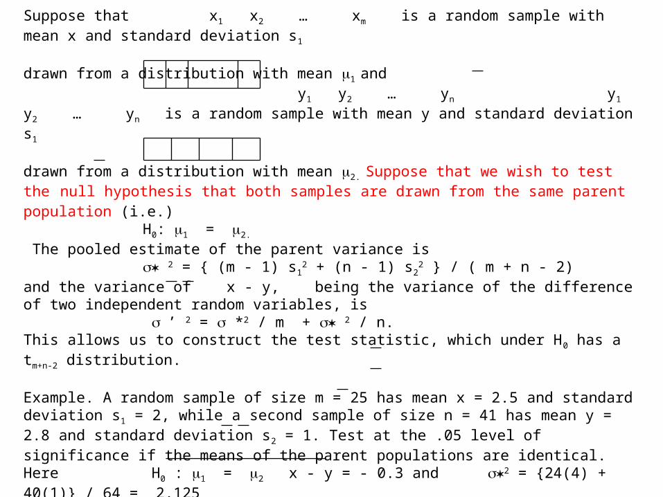
Testing Differences between Means

Suppose that x1 x2 … xm is a random sample with mean x and standard deviation s1

drawn from a distribution with mean 1 and y1 y2 … yn y1 y2 … yn is a random sample with mean y and standard deviation s1

drawn from a distribution with mean 2. Suppose that we wish to test the null hypothesis that both samples are drawn from the same parent population (i.e.)

H0: 1 = 2.

The pooled estimate of the parent variance is 2 = { (m - 1) s1

2 + (n - 1) s22 } / ( m + n - 2)

and the variance of x - y, being the variance of the difference of two independent random variables, is

’ 2 = *2 / m + 2 / n.This allows us to construct the test statistic, which under H0 has a tm+n-2 distribution.

Example. A random sample of size m = 25 has mean x = 2.5 and standard deviation s1 = 2, while a second sample of size n = 41 has mean y = 2.8 and standard deviation s2 = 1. Test at the .05 level of significance if the means of the parent populations are identical.Here H0 : 1 = 2 x - y = - 0.3 and 2 = {24(4) + 40(1)} / 64 = 2.125so the test statistic is

- 0.3 / The .05 critical value for Z(0, 1) isso the test is inconclusive

Paired Tests

If the sample values ( xi , yi ) are paired, such as the marks of students in two examinations, then let di = xi - yi be their differences and treat these values as the elements of a sample to generate a test statistic for the hypothesis

H0: 1 = 2.

The test statistic d / sd / n has a tn-1 distribution if H0 is true.

Example. In a random sample of 100 students in a national examination their examination mark in English is subtracted from their continuous assessment mark, giving a mean of 5 and a standard deviation of 2. Test at the .01 level of significance if the true mean mark for both components is the same.Here n = 100, d = 5, sd / n = 2/10 = 0.2so the test statistic is 5 / 0.2 = 10.the 0.1 critical value for a Z(0, 1) distribution is 2.58, so H0 is rejected at the .01 level of significance.

Tests for the Variance.

For normally distributed random variables, givenH0: 2 = k, a constant, then (n-1) s2 / k has a 2

n - 1 distribution.

Example. A random sample of size 30 drawn from a normal distribution has variance s2 = 5.Test at the .05 level of significance if this is consistent with H0 : 2 = 2 .Test statistic = (29) 5 /2 = 72.5, while the .05 critical value for 2

29 is 45.72, so H0 is rejected at the .05 level of significance.

Chi-Square Test of Goodness of Fit

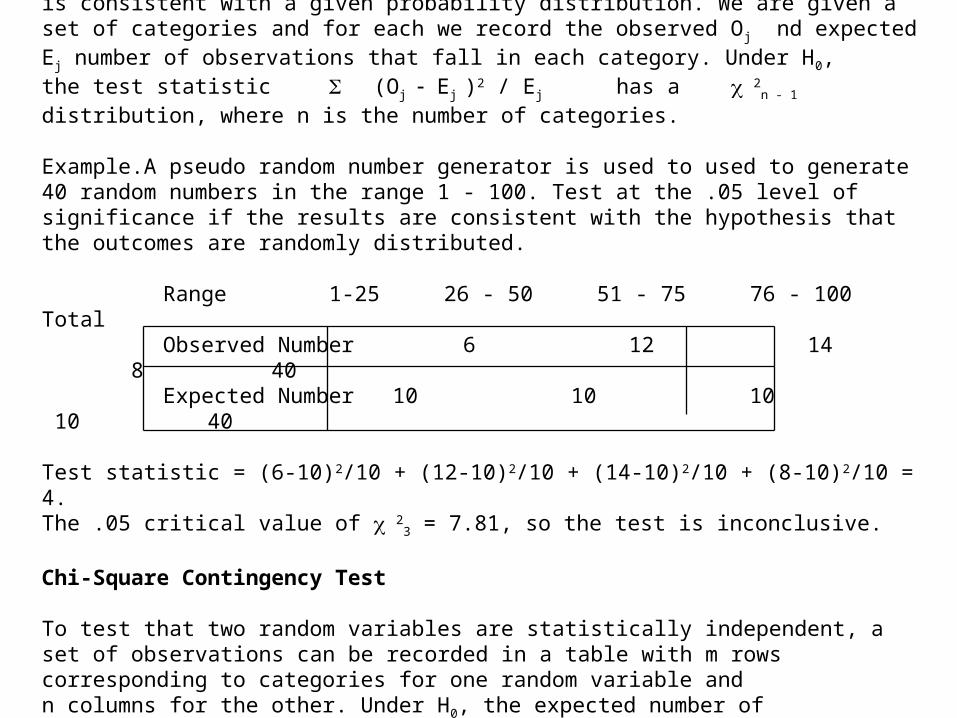
This can be used to test the hypothesis H0 that a set of observations is consistent with a given probability distribution. We are given a set of categories and for each we record the observed Oj nd expected Ej number of observations that fall in each category. Under H0,the test statistic (Oj Ej )2 / Ej has a 2

n - 1 distribution, where n is the number of categories.

Example.A pseudo random number generator is used to used to generate 40 random numbers in the range 1 - 100. Test at the .05 level of significance if the results are consistent with the hypothesis that the outcomes are randomly distributed.

Range 1-25 26 - 50 51 - 75 76 - 100 Total Observed Number 6 12 14 8 40 Expected Number 10 10 10 10 40

Test statistic = (6-10)2/10 + (12-10)2/10 + (14-10)2/10 + (8-10)2/10 = 4.The .05 critical value of 2

3 = 7.81, so the test is inconclusive.

Chi-Square Contingency Test

To test that two random variables are statistically independent, a set of observations can be recorded in a table with m rows corresponding to categories for one random variable and n columns for the other. Under H0, the expected number of observations for the cell in row i and column j is the appropriate row total by the column total divided by the grand total. Under H0, the test statistic (Oij Eij )2 / Eij has a 2

(m -1)(n-1) distribution.

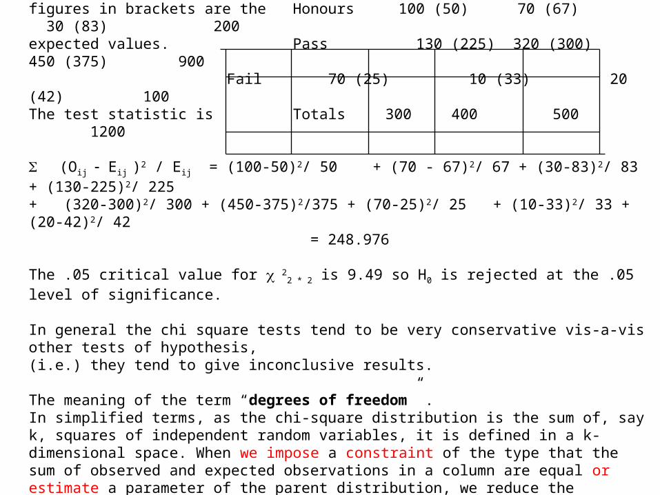
Chi-Square Contingency Test - Example

In the following table, the Results Maths History Geography Totalsfigures in brackets are the Honours 100 (50) 70 (67) 30 (83) 200expected values. Pass 130 (225) 320 (300) 450 (375) 900

Fail 70 (25) 10 (33) 20 (42) 100The test statistic is Totals 300 400 500 1200

(Oij Eij )2 / Eij = (100-50)2/ 50 + (70 - 67)2/ 67 + (30-83)2/ 83 + (130-225)2/ 225+ (320-300)2/ 300 + (450-375)2/375 + (70-25)2/ 25 + (10-33)2/ 33 + (20-42)2/ 42 = 248.976

The .05 critical value for 22 * 2 is 9.49 so H0 is rejected at the .05 level of significance.

In general the chi square tests tend to be very conservative vis-a-vis other tests of hypothesis,(i.e.) they tend to give inconclusive results.

The meaning of the term “degrees of freedom” .In simplified terms, as the chi-square distribution is the sum of, say k, squares of independent random variables, it is defined in a k-dimensional space. When we impose a constraint of the type that the sum of observed and expected observations in a column are equal or estimate a parameter of the parent distribution, we reduce the dimensionality of the space by 1. In the case of the chi-square contingency table, with m rows and n columns, the expected values in the final row and column are predetermined, so the number of degrees of freedom of the test statistic is (m-1) (n-1).