Data Analysis (534) Please turn on your cameras.

Data Analysis (534)

Please turn on your cameras.

Textbook: Modern Applied Statistics with S, 4th ed.

by Venables and RipleyOffice: WH 132Office hours: M 3:30pm-4:30pm, Tu 7:00pm-8:00pmClassroom: On-line 1:10-2:10pmHomework due: Wednesday before class.

Email me at [email protected] before 1:10pm on Wednesday.Grading policy: 40% homework+10% quizzes + 20% midterm+30% final.

B = 75 ±Midterm: Mar. 29 (M)Final: May 25 10:25am-12:25pm

You can bring one page with R commands and formulas in exams.

During quizzes or exams, use another camera that can show your table, screen andyou.Quiz: Once a week at a random day,

quiz problems: formulas for Math 447-448 (see my website)right after quiz, take a picture of your answer, output as a pdf file and email me.

Homework assigned during a week is due next Wednesday.It is on my website: http://www.math.binghamton.edu/qyu/qyu personal

Remind me if you do not see it by Saturday morning !The lecture note is also on my website

http://www.math.binghamton.edu/qyu/qyu personal

note and note2 are updated one,Chapter 0. Introduction.

Data analysis is to teach how to analyze data (using R program). Usual steps in dataanalysis:

1. For a random sample, e.g., regression data,

(Xi, Yi), i = 1, ..., n, input them to a computer software, say R or S-plus.

2. Assume a proper probability model, say a parametric modelYi = β′Xi + ǫi, where ǫ ∼ N(α, σ2);

or a semiparametric modelYi = β′Xi + ǫi, where ǫ ∼ F , an unknown cumulative distribution function (cdf),

or a non-parametric model(Xi, Yi) ∼ F (x, y), where F is unknown.

3. Compute an estimate of (α, β, σ) if it is parametric,

or an estimate of (β, F ) if it is semi-parametric,

or an estimate of F , if it is non-parametric.

4. Check whether the model assumption is valid.

5. If No, go to Step 2, otherwise, carry out the other statistics inferences, e.g.,

testing statistical hypotheses,

or constructing confidence intervals,

or drawing inferences on some other parameters, e.g. P (Y ∈ A|X = x) = ?.

Example 1. An example how to hand in homework.Xi: 1 2 3 4 5 6 7 8 9 10 11 12 13 14 15 16 17 18 19 20

1

21 22 23 24 25 26 27 28 29 30Yi: 1.40 1.40 3.36 4.69 6.05 7.35 7.27 6.80 8.94

8.68 11.24 11.62 12.85 14.38 14.28 15.43 16.86 18.08 18.4519.73 20.63 20.73 23.30 23.06 26.15 27.45 27.67 27.64 28.28 32.30

Suppose it is in a file called “data” in a directory /home/qyu/try in a PC.cd /home/qyu/try

Two ways to work on R:1. Write a program file, say ch0,

R - -vanilla < ch0 # figure is in the file Rplots.pdfR - -vanilla < ch0 > output # all commands and output in the file called “output”.

2. Open R in that directory directly by typing:R or click the icon of R on a laptop.

You can find R download site through Google.Or login to department computer.ssh [email protected] (ssh2, ssh3)sftp [email protected]

> library(MASS)> sink(”ch0.out”) # put output in ch0.out file> x=matrix(scan(”data”), ncol=1, byrow=T)> y=x[31:60]> x=x[1:30]> z=lm(y∼x)> summary(z)> plot(x,y) # scatter plot> plot(fitted(z),studres(z))> qqnorm(studres(z))> qqline(studres(z))> makepsfile = function()

ps.options(horizontal = F)ps.options(height=4.0, width=7.5)postscript(”ch1.ps”)par(mfrow =c(1,3))plot(x,y)plot(fitted(z),studres(z))qqnorm(studres(z))qqline(studres(z))dev.off()

> makepsfile()> sink() # close sink function> rm(x,y)> q()

The output is as follows.Call:lm(formula = y ∼ x)Residuals:

2

Min 1Q Median 3Q Max-1.3470 -0.5934 -0.1120 0.4434 2.1720Coefficients:

Estimate Std. Error t value Pr(> |t|)(Intercept) −0.06299 0.32684 −0.193 0.849x 1.00636 0.01841 54.663 < 2e− 16 ∗ ∗∗

—

Signif. codes: 0 *** 0.001 ** 0.01 * 0.05 . 0.1 1Residual standard error: 0.8728 on 28 degrees of freedomMultiple R-squared: 0.9907, Adjusted R-squared: 0.9904F-statistic: 2988 on 1 and 28 DF, p-value: < 2.2e-16

0 5 10 15 20 25 30

51

01

52

02

53

0

x

y

0 5 10 15 20 25 30

−1

01

23

fitted(z)

stu

dre

s(z

)

−2 −1 0 1 2

−1

01

23

Normal Q−Q Plot

Theoretical Quantiles

Sa

mp

le Q

ua

ntile

s

Write a report using Tex (or LaTex).Edit a file called report.tex (see example),need a postscript file: ch1.ps (which is created by makepsfile in page 2),attach relevant R outputs into your report (see the sample homework I email you).

Some commands in the linex system:tex report.tex (create report.dvi file) (or latex ..., or pdflatex ...)xdvi report (view the file)dvipdf report (create a pdf file)dvips report -o report.ps (create a postscript file)dvips -p 2 -l 3 report -o page2.psps2pdf page2.ps (create a two-page pdf file)pdf2ps report.pdf

For each homework, send me 3 files by email (do not compress them):1. junk.pdf — the formal report file (pdf file)2. junk.tex – the Tex file preparing junk.pdf3. junk —- a dos file collecting R commands used and output of R.You need to orgainize them so that they are readable.A brief manual for Latex is on my website: short-math-guideA brief introduction of R is in given in Math 531One can google the pdf file “An introduction to R”.

A sample of homework was emailed to you. Mimic it in your homework.

Chapter 5. Univariate Statistics5.1. Probability Distributions.

Let X be a random variable (rv).

3

Its cdf F (t) = PX ≤ t, domain ?

density function (df) f(t) =

F ′(t) if X is continuousF (t) − F (t−) if X is discrete,

domain ?

quartile Q(u) = F−1(u) = mint : F (t) ≥ u domain ?survival function S(t) = 1 − F (t).

Example 1. X ∼ Weibull distribution with cdf F (x|γ, τ) = 1 − exp(−(x/τ)γ), x > 0,S(x|γ, τ) = exp(−(x/τ)γI(x > 0)) and E(X) =

∫xf(x)dx = τΓ(1 + 1/γ))

γ– shape, τ – scale,pweibull(x,shape,scale) — F (x),qweibull(x,shape,scale) — Q(x),dweibull(x ,shape,scale) — f(x),rweibull(10 ,1 ,3 ) — 10 observations from Exp(3) with E(X) = 3.

Remark. The list of all distributions is given in Table 5.1.

Distributions R name parameters f(x; θ)

beta beta shape1, shape2 xα−1(1−x)β−1

B(α,β) , x ∈ (0, 1)

uniform unif min,max 1b−a , x ∈ (a, b)

gamma gamma shape, scale xα−1e−x/β

Γ(α)βα , x, α, β > 0

exponential exp rate ρe−ρx, x > 0chi− square chisq dfCauchy cauchy location, scale 1

π(1+x2) → 1β f(x−α

β )

binomial binom size, prob(nx

)px(1 − p)n−x, x ∈ 0, 1, ..., n

negative binomial nbinom size, probgeometric geom prob p(1 − p)x, x = 0, 1, ...

hypergeometric hyper m, n, knormal norm mean, sd

log − normal lnorm meanlog, sdlogF f df1, df2T t df

logistic logis location, scalePoisson pois lambdaWeibull weibull shape, scaleWilcox wilcox m, n

Example 1 (contitued).R> x=rweibull(100,1,5)> round(x,2)> mean(x)Q: What will you see ?QQplot: quantile-quantile plot.

1. Given data Xi, i = 1, ..., n.2. Order them as X(1) ≤ · · · ≤ X(n).

3. Plot (X(i), F−1(F (X(i)))), where F is a step function, and

F (X(i)) = in (ecdf), or

i− 12

n (ppoints(x)), or in+1 .

Since F (t) → F (t) w.p.1, we expect the qqplot is roughly a straight line.

4

Remark. If the assumption Xi ∼ F is correct(and thus F = F in the ideal situation),then qqplot is plotting (Xi, Xi), i = 1, ..., n, as F−1(F (Xi)) = Xi.Thus the qqplot is expected to be a straight line roughly.

Example 2. Given X1, ..., X100, 100 observations in the file data ex2,Estimate F and PX ∈ (1, 2] and E(X).It is desirable to do parameteric analysis, say assume that they are from aWeibull distribution. F (x|γ, τ) = 1 − exp(−(x/τ)γ), x > 0

Solution: We first find the MLE of (γ, τ), that is,a value of (γ, τ) that maximizes the joint density functionL(γ, τ) =

∏ni=1 f(Xi|γ, τ), where f(t) = F ′(t), t > 0.

Carry out data analysis using R codes:x=matrix(scan(”data ex2”), ncol=1, byrow=T)summary(x)y=fitdistr(x,“weibull”) # compute MLE

Remark. Distributions ”beta”, ”cauchy”, ”chi-squared”, ”exponential”, ”gamma”, ”geometric”,”log-normal”, ”lognormal”, ”logistic”, ”negative binomial”, ”normal”, ”Poisson”, ”t”and ”weibull” are recognised, case being ignored.ysummary(y)pweibull(2,y$e[1],y$e[2])-pweibull(1,y$e[1],y$e[2]) # P (X ∈ (1, 2])(y$e[2])*gamma(1+1/y$e[1]) # E(X) =

∫xf(x)dx = τΓ(1 + 1/γ))

Output:> summary(x)

V1Min. :1.0301st Qu.:1.840Median :3.000Mean :2.9923rd Qu.:4.070Max. :4.970

> yshape scale2.7761986 3.3746473(0.2257762) (0.1280903)

> summary(y) different from summary(lm())Length Class Mode

estimate 2 −none− numericsd 2 −none− numericvcov 4 −none− numericloglik 1 −none− numeric #loglikelihoodn 1 −none− numeric

Question: What is the use of summary(y) here ?> y$estimate

shape scale2.776199 3.374647

> y$eshape scale

5

2.776199 3.374647> y$v # y$vcov

shape scaleshape 0.050974887 0.009118663scale 0.009118663 0.016407135

> pweibull(2, 2.776,3.3746)-pweibull(1, 2.776,3.3746)) # P (X ∈ (1, 2])[1] 0.1750694

> pweibull(2,y$e[1],y$e[2])-pweibull(1,y$e[1],y$e[2])[1] 0.1750694

> ((y$e[2])*gamma(1+1/y$e[1])) # E(X)3.003995

Ans: The MLEs under the Weibull model are τ = 3.4 with στ = 0.13and γ = 2.8 with σγ = 0.23.

F (t) = 1 − exp(−(t/3.4)2.8), t > 0 and P (X ∈ (1, 2]) ≈ 0.175.E(X) = τΓ(1 + 1/γ) ≈ 3.004 verses X = 2.992.

Question:1. Can the model be simplified ?

e.g., X ∼ Exp(1)? (τ = 1 or γ = 1 as F (x) = 1 − e−( xτ )γ , x > 0).

If the model is valid, then it can be shown that the MLEs γ and τhave approximately normal distributions, N(γ, σ2

γ) and N(τ, σ2τ ).

H0: γ = 1 v.s. H1: γ 6= 1. Check |γ − 1| < 2σγ ?H0: τ = 1 v.s. H1: τ 6= 1. Check |τ − 1| < 2στ ?Ans: It seems that the model cannot be simplified Why ?

2. E(X) = τΓ(1 + 1/γ) ≈ 3.004 is the MLE of E(X) and

X = 2.992 is the non-parametric estimator of E(X) (X =∑

i xf(x), where

f(x) =∑n

i=1 1(Xi = x)/n is the density of the edf F (x) =∑n

i=1 1(Xi ≤ x)/n,a non-parametric MLE (NPMLE) of FX(t). Which is better ?

3. Is the model assumption valid ?We can use the qqplot, confidence band (CB) of the edf and ks.test to check.CB of the edf is the pointwise confidence interval based on the edf.

Example of qqplot and CB codes:makepsfile = function() ps.options(horizontal = F)ps.options(height=8.0, width=7.5)postscript(”ch1.2.ps”)par(mfrow =c(2,2))x=sort(x)plot(x,pweibull(x,y$e[1],y$e[2]),type=”l”,lty=2)lines(x,ppoints(x),type=”S”,lty=3)s=1.96*sqrt(ppoints(x)*(1-ppoints(x))/100)lines(x,ppoints(x)+s,type=”S”,lty=3)lines(x,ppoints(x)-s,type=”S”,lty=3)leg.names=c(”CB”, ”weib”)legend(3, 0.3, leg.names, lty=c(3,2),cex=1.0)t=(0:70)/10plot(t,pweibull(t,y$e[1],y$e[2]),type=”l”,lty=2)lines(x,ppoints(x),type=”S”,lty=3)s=1.96*sqrt(ppoints(x)*(1-ppoints(x))/100)

6

lines(x,ppoints(x)+s,type=”S”,lty=3)

lines(x,ppoints(x)-s,type=”S”,lty=3)

lines(c(0,1),c(0,0),type=”l”,lty=3)

lines(c(5,7),c(1,1),type=”l”,lty=3)

leg.names=c(”CB”, ”weib”)

legend(3, 0.3, leg.names, lty=c(3,2),cex=1.0)

u=rweibull(100,y$e[1],y$e[2])

plot(qweibull(ppoints(x),y$e[1],y$e[2]),x) # or qqplot(u,x) compare weibull to data

z=qweibull((1:100)/101,y$e[1],y$e[2])

qqplot(u,z) # compare to qqplot weibull v.s. weibull

dev.off()

makepsfile()

> pweibull(1,y$e[1],y$e[2]) +1-pweibull(5,y$e[1],y$e[2])

[1] 0.08444813

1 2 3 4 5

0.0

0.2

0.4

0.6

0.8

1.0

x

pp

oin

ts(x

)

CBweib

0 1 2 3 4 5 6 7

0.0

0.2

0.4

0.6

0.8

1.0

t

pw

eib

ull(

t, y

$e

[1],

y$

e[2

])

CBweib

1 2 3 4 5 6

12

34

5

qweibull(ppoints(x), y$e[1], y$e[2])

x

1 2 3 4 5

12

34

56

u

z

Fig(1, 1) : similar to next F ig(1, 2) : cdf of weibull v.s. edf with its confidence bandFig(2, 1) : qqplot weibull F ig(2, 2) : qqplot of 100 data from Weibull

Figure 5.1.

It seems that the Weibull assumption is not valid.qqplot is quite subjective.

ks.test in R is a test.Kolmogorov-Smirnov Goodness-of-Fit Test

Performs a one or two sample Kolmogorov -Smirnov test, which tests the relationshipbetween two distributions.One-sample. Suppose that X1, ..., Xn are a random sample from F .

7

ks.test(x, “pweibull”, shape, scale)H0: F = Fo a Weibull distribution(shape,scale), verseH1: F 6= Fo, where Fo is given (together with the parameter).

The test statistic is one sided test 1(D > c), where D = sup|F (t) − Fo(t)| : t ∈ R.(can we use a two-sided test 1(D /∈ [c1, c2]) ?Remark. P-value= PD > Do (given in R),

where Do is the observed value of D for the given X1, ..., Xn.We reject H0: F = Fo(·|θ) assuming θ is known if P-value is small (< 0.05). θ = ?> ks.test(x, ”pweibull”, y$e[1],y$e[2])

One-sample Kolmogorov-Smirnov testdata: xD = 0.0965, p-value = 0.3094alternative hypothesis: two-sided

Question: What is our conclusion about the test ?Does it agree with qqplot ?

Remark. In ks.test, the P-value is asymptotically true. Thus it is assumed that(1) θ is the true value and(2) the sample size n is very large.

However, θ is estimated by its MLE here and n is not large, this changed its true P-value.One can find the critical value in D by empirical quantiles of 0.05 for a given sample size n.

(See the simulation exercises in Examples 3, 4 and 5.)Example 3. Generate data from U(1,5) with n = 100 or 1000.Test against Weibull, Uniform and Uniform(1,5) with ks(). Why uniform of U(1,5) ?Question: What is the difference between the last two tests ?Summarize the findings.How to find the MLE of the parameter θ for:

Weibull ? θ ? true value of θ ?Uniform ? θ ? true value of θ ?> (y=fitdistr(x,”unif”))

Error in fitdistr(x, ”unif”) : unsupported distributionMLE of U(a,b) ?

Uniform(1,5) ?> fun3 = function(n)

x=runif(n,1,5)y=fitdistr(x,”weibull”)a=ks.test(x, ”pweibull”, y$e[1], y$e[2])b=ks.test(x, ”punif”, min(x),max(x))c=ks.test(x, ”punif”, 1, 5)return(c(u=a$p.value, v=b$p, w=c$p))

> fun3(100) # What is the output ? What do you expect ?u v w

0.4267747 0.7190210 0.6058055 Are they expected ?? ? ? Is it possible ?

Repeat 1000 times:m=1000u=rep(0,m)v=rep(0,m)w=rep(0,m)

8

for(i in 1:m) z=fun3(n)u[i]=as.numeric(z[1]<0.05)v[i]=as.numeric(z[2]<0.05)w[i]=as.numeric(z[3]<0.05)

mean(u)[1] 0.013 # (Power or size of the test φ ?

︸︷︷︸

E(φ(U)) or P(H1|Ho)

Or an estimate ?)

mean(v)[1] 0.043 # (Power or size of the test ? Or an estimate ?)mean(w)[1] 0.044 # (Power or size of the test ? Or an estimate ?)n=1000 # Repeat but with larger sample size n sizeu=rep(0,m)v=rep(0,m)w=rep(0,m)for(i in 1:m) z=fun3(n)u[i]=as.numeric(z[1]<0.05)v[i]=as.numeric(z[2]<0.05)w[i]=as.numeric(z[3]<0.05)>c(mean(u), mean(v), mean(w))[1] 1 0.05 0.053 # Are they expected ?

Summary: Uniform(1,5) data test forWeibull Uniform Uniform(1, 5)

n P (H0|H1) P (H1|H0) P (H1|H0)ideal 0 0.05 0.051000 0 why ? 0.05 0.053100 0.987 ? 0.043 0.044

Findings:1. If n is very large, then it seems that ks.test works.2. OW, P (H0|H1) can be 99%, instead of < 50%, this explains the discrepancy in Ex. 2.3. If n is moderate, the level of the ks.test seems fine.

Remark. The P-value given in ks.test is an approximation when n is very large. Otherwise,it is arbitrary.

Example 4. Generate data from Weibull(1,0.2) with n = 100 or 1000.Test against Weibull and Weibull(1,0.2). Summarize the findings.

R codes:fun3 = function(n)

x=rexp(n,5) # Why not rexp(n,0.2) ?y=fitdistr(x,”weibull”)a=ks.test(x, ”pweibull”, y$e[1], y$e[2]) true value of (γ, τ) ?c=ks.test(x, ”pweibull”, 1, 0.2) (y$e[1], y$e[2]) = (1, 0.2) ?

9

return(c(u=a$p.value, w=c$p))n=100fun3(n)output:

u w0.4647952 0.5927737

Are they what you expect ?

Repeat 1000 times again.

m=1000

u=rep(0,m)

w=rep(0,m)

for(i in 1:m) z=fun3(n)

u[i]=as.numeric(z[1]<0.05)

w[i]=as.numeric(z[2]<0.05)

> c(mean(u) , mean(w))

[1] 0 0.045What happens if n is larger ?

n=1000

u=rep(0,m)

w=rep(0,m)

for(i in 1:m) z=fun3(n)

u[i]=as.numeric(z[1]<0.05)

w[i]=as.numeric(z[2]<0.05)

> c(mean(u) , mean(w))

[1] 0 0.046Remark. The above code can be revised by R code apply(), which is faster.Summary: Weibull(1,0.2) data test for

Weibull Weibull(1, 0.2)n P (H1|H0) P (H1|H0)50 0 0.045

1000 0 0.046ideal 0.05 0.05

Finding: P (H1|H0) = 0 if Weibull data test Weibull with (τ, γ) replaced by the MLE.It is too small or the critical value for size 0.05 is too large.

Notice that for a test φ if P (H1|H0) = 0, then it is often P (H0|H1) = ??

Examples 3 and 4 suggest that ks.test is not reliable for n = 100.

Example 2 (continued). Examples 3 and 4 suggest that one needs to modify the ks.testfor the case θ is replaced by the MLE.

The test statistic is D = supt |F (t) − Fo(t)| if H1 : F (t) 6= Fo(t).How to find the empirical critical value of size 0.05 for ks.test:

x=matrix(scan(”data ex2”), ncol=1, byrow=T)

y=fitdistr(x,”weibull”))

10

b=ks.test(x, ”pweibull”, y$e[1], y$e[2])$s # What is b ?Ans:

z=ks.test(x, ”pweibull”, y$e[1], y$e[2]), u=rep(0,1000)summary(z)

Length Class Modestatistic 1 −none− numericp.value 1 −none− numeric

alternative 1 −none− charactermethod 1 −none− character

data.name 1 −none− character

for (i in 1:1000)x=rweibull(100, y$e[1], y$e[2])z=fitdistr(x,”weibull”)a=ks.test(x, ”pweibull”, z$e[1], z$e[2])u[i]=a$s

> sort(u)[950] # what is this ?

[1] 0.08622978> b b= ks.test(x, ”pweibull”, y$e[1], y$e[2])

[1] 0.09650574 # Do= 0.09650574Q: Can we have conclusion now ?> mean(u>b)

# what is this ?[1] 0.024

What is the reasoning of this approach ?1. First derive the test statistic value b from the data.2. Pretend the true θ =MLE to generate pseudo random numbers.3 Repeat the ks.test m times with the same n and unknown θ.4. It results i.i.d. ks.test statistic value Di, i = 1, ..., m5. SLLN (1(D > b) → P (D > b) anything wrong ??).

What is conclusion for testing H0: the data are from Weibull distribution in Ex. 2 ?Question: Ideally, if we reject H0 when ks.test$p < 0.05, the size of the test is ??How to find a “ks.test$<?? for a size 0.05 for the data in Ex. 2 ?Ans:

x=matrix(scan(”data ex2”), ncol=1, byrow=T)y=fitdistr(x,”weibull”))for (i in 1:10000)

x=rweibull(100, y$e[1], y$e[2])z=fitdistr(x,”weibull”)a=ks.test(x, ”pweibull”, z$e[1], z$e[2])u[i]=as.numeric(a$p<0.05) # mean(u)=0.00u[i]=as.numeric(a$p<0.43) # try to increase from 0.05 to achieve mean(u)≈ 0.05

mean(u)[1] 0.0494 (≈ 0.05)Since the ks.test and qqplots suggest that the data are not from a Weibull distribution.

Then there are two choices:

11

1. empirical distribution function (edf),2. other parametric distributions.

1. Use the edf to estimate F , F (t) = 1n

∑ni=1 1(Xi ≤ t).

R codes:mean(x)sum((x>1& x<=2))/length(x) mean((x>1& x<=2))

Outcomes: µ = X = 2.99 and P (X ∈ (1, 2]) = 0.292. Try other parameteric cdf’s,

Notice that in the program fitdistr(), distributions ”beta”, ”cauchy”, ”chisq”, ”exp”,”f”, ”gamma”, ”geom”, ”lnormal”, ”logis”, ”nbinom”, binom”, ”norm”, ”pois”, ”t” and”weibull” are recognised.Which of them are inapproprite ? Notice that (X(1), X(n)) ⊂ (1, 5).

beta ? cauchy ?geom ? nbinom ? binom ? pois ?

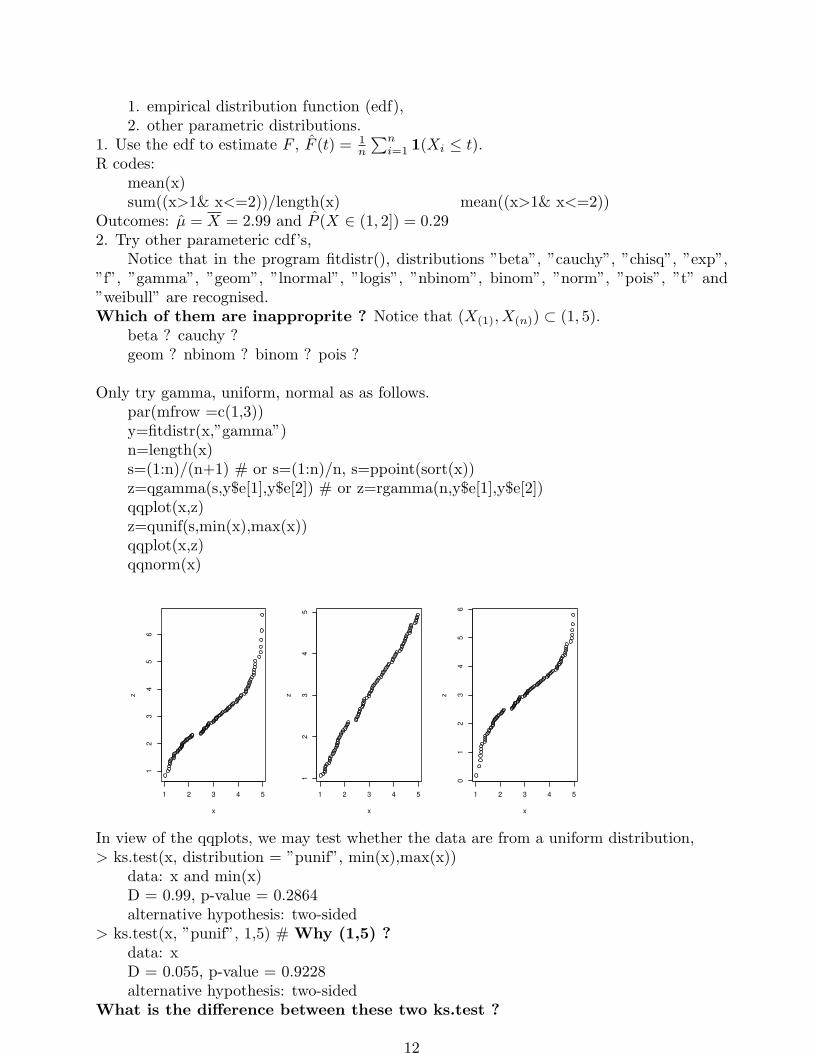
Only try gamma, uniform, normal as as follows.par(mfrow =c(1,3))y=fitdistr(x,”gamma”)n=length(x)s=(1:n)/(n+1) # or s=(1:n)/n, s=ppoint(sort(x))z=qgamma(s,y$e[1],y$e[2]) # or z=rgamma(n,y$e[1],y$e[2])qqplot(x,z)z=qunif(s,min(x),max(x))qqplot(x,z)qqnorm(x)

1 2 3 4 5

12

34

56

x

z

1 2 3 4 5

12

34

5

x

z

1 2 3 4 5

01

23

45

6

x

z

In view of the qqplots, we may test whether the data are from a uniform distribution,> ks.test(x, distribution = ”punif”, min(x),max(x))

data: x and min(x)D = 0.99, p-value = 0.2864alternative hypothesis: two-sided

> ks.test(x, ”punif”, 1,5) # Why (1,5) ?data: xD = 0.055, p-value = 0.9228alternative hypothesis: two-sided

What is the difference between these two ks.test ?

12

Which is more appropriate ?Example 3 suggests that if X ∼ U(a, b), both work for n = 100.Example 4 suggests that if X ∼ Weibull, MLE does not work for n = 100.

Can we assume X ∼ U(a, b) ?

F (t) =

t−ab−a if t ∈ (a, b),1 if t ≥ b.

then the MLE is (a, b) = (miniXi,maxiXi) = (1.03, 4.97),as it maximizes the likelihood function L(a, b) =

∏ni=1

1b−a1(Xi ∈ (a, b)).

R codes:(max(x)+min(x))/2punif(2,min(x),max(x))-punif(1,min(x),max(x))

Or assume X ∼ U(1, 5) based on ks.test(x,“unif”, 1,5).Final solution:

F is U(1, 5).µ = 3 andP (X ∈ (1, 2]) = 0.25

Comments: Various estimates of P (X ∈ (1, 2]) = 0.25 and their SE’s are as follows.

1. edf=> P (X ∈ (1, 2]) = 0.29, with SE

√

P (1 − P )/n ≈ 0.045.

and with CI [0.20, 0.38] difference between SE and SD ?)

2. U(a,b) (assuming (a, b) ⊃ (1, 2)) => Z = P (X ∈ (1, 2]) = (2 − 1)/(b − a) ≈ 0.254SEZ ≈ ? HW)

Hint: (a, b) = (X(1) ∧ 1, X(n) ∨ 2), σ2Z = ? fX(1),X(n)

(x, y) = ??

3. U(a,b) => Z = P (X ∈ (1, 2]) =(2∧b−1∨a)1(X(1),X(n))∩(1,2) 6=∅)

b−a, (SEZ ≈ ? HW)

Hint: (a, b) = (X(1), X(n)), σ2Z = ? fX(1),X(n)

(x, y) = ??4. U(1,5) => P (X ∈ (1, 2]) = 0.25, SD = ?5 Weibull MLE=> P (X ∈ (1, 2]) = 0.18, differ≈ half due to wrong assumption.

Question: # of parameters using the EDF ? (non-parametric model)# of parameters using the uniform distribution ? (parametric model)

Both models are correct, but there are more parameters in the edf.Homework:(1) Compare the lengths of the CI of P (X ∈ (1, 2]) due to the EDF and the CI under the

Weibull distribution for the given data in Ex. 2. Check whether P (X ∈ (1, 2]) fallsin the CI of P (X ∈ (1, 2]) due to the EDF or under the Weibull assumption ? Thenexplain what it implicates. The data are:1.39 3.63 2.06 4.25 2.76 4.64 1.85 1.72 1.37 1.64 4.01 3.25 1.14 4.70 4.691.73 2.57 3.96 3.12 3.55 1.77 1.62 2.02 1.39 4.93 2.14 1.52 2.80 3.67 3.014.95 1.45 4.41 4.06 3.09 2.08 3.51 4.92 4.48 4.97 4.51 4.45 3.21 4.68 1.711.39 4.32 1.86 4.64 3.15 2.13 4.39 1.56 2.61 2.71 4.66 3.48 3.38 1.20 2.901.94 2.99 3.10 2.52 2.60 2.77 2.56 1.03 4.91 1.23 1.22 3.96 1.81 1.92 1.692.62 2.48 2.73 3.31 3.79 4.86 4.46 1.22 3.92 3.77 1.20 2.47 3.03 1.27 3.582.78 4.13 4.31 4.55 3.73 3.34 4.10 1.70 4.32 1.55

(2) Compute the SD in the above Comment 2.Example 5. Generate 100 data from Exp(1/2) with mean 1/2.Now pretend that we do not know the underlying distribution of the data. Assume Weibulldistribution. Estimate F and PX ∈ (1, 2] and E(X).Sol. Simulation data:

13

> x=rexp(100,2)> mean(x)

[1] 0.5153382 # rate =2 or scale=2 ?Now pretend we assume but do not really know the true distribution is

F (t) = 1 − exp(−(t/τ)γ), t > 0.The MLE is computed:

>fitdistr(x,”weibull”)shape scale

1.16690389 0.54517822(0.08866768) (0.04934344)

We may testHo: γ = 1 v.s. H1: γ 6= 1,orHo: τ = 1 v.s. H1: τ 6= 1.That is, we check whether the data is from Exp(µ) or further Exp(1).

If X ∼Weibull(γ, τ), µ = τΓ(1 + 1/γ) with 2 parameters and SE by Delta method;Note: Γ(α) =

∫∞0tα−1e−tdt, Γ′(α) =

∫∞0

(lnt)tα−1e−tdt can be computed numerically,

If X ∼ Exp(µ), µ = X with 1 parameter and SE= σX/n=?If X ∼ Exp(1), µ = 1 with no parameter and SE=?

Conclusion ?

µX = 0.55 or µX = 0.52 ?

σµX= ? σµX

= 0.52/10 why ? which is smaller ? why ?

F (t) = 1 − e−t/0.52, t > 0.P (X ∈ (1, 2)) = e−1/0.52 − e−2/0.52.

Done ?

14

0.0 0.5 1.0 1.5 2.0 2.5

0.0

0.2

0.4

0.6

0.8

1.0

ecdf(x)

x

Fn

(x)

0.0 0.5 1.0 1.5 2.0 2.5

0.0

0.2

0.4

0.6

0.8

1.0

x

pp

oin

ts(x

)

0.0 0.5 1.0 1.5 2.0

0.0

0.5

1.0

1.5

2.0

2.5

qweibull(ppoints(x), y$e[1], y$e[2])

sort

(x)

0 1 2 3 4 5

0.0

0.5

1.0

1.5

2.0

2.5

qexp(ppoints(x))

sort

(x)

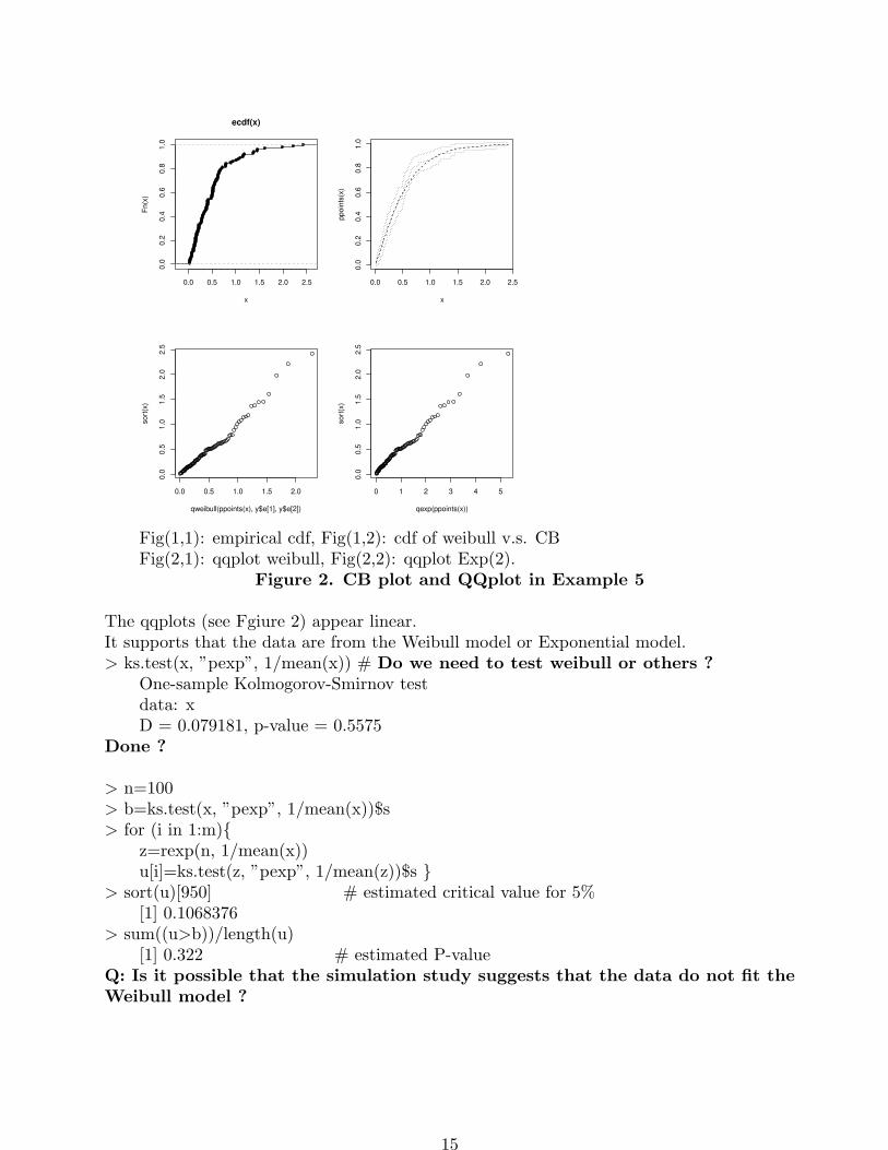
Fig(1,1): empirical cdf, Fig(1,2): cdf of weibull v.s. CBFig(2,1): qqplot weibull, Fig(2,2): qqplot Exp(2).

Figure 2. CB plot and QQplot in Example 5

The qqplots (see Fgiure 2) appear linear.It supports that the data are from the Weibull model or Exponential model.> ks.test(x, ”pexp”, 1/mean(x)) # Do we need to test weibull or others ?

One-sample Kolmogorov-Smirnov testdata: xD = 0.079181, p-value = 0.5575

Done ?

> n=100> b=ks.test(x, ”pexp”, 1/mean(x))$s> for (i in 1:m)

z=rexp(n, 1/mean(x))u[i]=ks.test(z, ”pexp”, 1/mean(z))$s

> sort(u)[950] # estimated critical value for 5%[1] 0.1068376

> sum((u>b))/length(u)[1] 0.322 # estimated P-value

Q: Is it possible that the simulation study suggests that the data do not fit theWeibull model ?

15

Example 6. Use Prostate data to fit the linear regression model y=lm(lpsa∼lweight).library(MASS)>library(faraway)>prostate[96:98, ]

lcavol lweight age lbph svi lcp gleason pgg45 lpsa96 2.882564 3.7739 68 1.558145 1 1.55814 7 80 5.4775197 3.471967 3.9750 68 0.438255 1 2.90417 7 20 5.58293>(y=lm(lpsa∼lweight,data=prostate))> summary(y)

Estimate Std. Error t value Pr(> |t|)(Intercept) −0.5281 0.8220 −0.642 0.522120lweight 0.8231 0.2230 3.691 0.000373

The model is y = −0.5281 + 0.8231x+ ǫ, where ǫ ∼ N(0, σ2).>lm(lpsa∼lweight-1,data=prostate)$co why do this ?

0.6811The model is y = 0.68x+ ǫ, where ǫ ∼ N(0, σ2). Done ?We need to check whether

(1) whether the model Y = α+ βx+ ǫ is valid;(2) whether ǫ ∼ N(0, σ2).

> x=y$resid> sd(x)

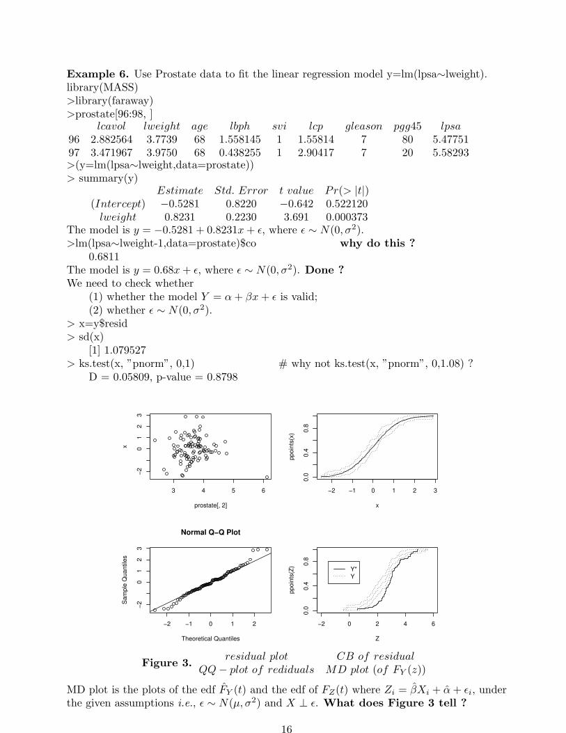
[1] 1.079527> ks.test(x, ”pnorm”, 0,1) # why not ks.test(x, ”pnorm”, 0,1.08) ?

D = 0.05809, p-value = 0.8798

3 4 5 6

−2

01

23

prostate[, 2]

x

−2 −1 0 1 2 3

0.0

0.4

0.8

x

ppoin

ts(x

)

−2 −1 0 1 2

−2

01

23

Normal Q−Q Plot


Sam

ple

Quantile

s

−2 0 2 4 6

0.0

0.4

0.8

Z

ppoin

ts(Z

)

Y*Y

Figure 3.residual plot CB of residual

QQ− plot of rediduals MD plot (of FY (z))

MD plot is the plots of the edf FY (t) and the edf of FZ(t) where Zi = βXi + α+ ǫi, underthe given assumptions i.e., ǫ ∼ N(µ, σ2) and X ⊥ ǫ. What does Figure 3 tell ?

16

For comparison, using the MLE of the parameter derive above, we generate simulateddata and give a similar plots in Figure 4.

−4 −3 −2 −1 0 1 2

0.0

0.4

0.8

x

ppoin

ts(x

)

−2 −1 0 1 2

−4

−2

01

2

Normal Q−Q Plot


Sam

ple

Quantile

s

0 1 2 3 4 5

02

46

Y

Z

−2 0 2 4 6

0.0

0.4

0.8

Z

ppoin

ts(Z

)

Y*Y

Figure 4.CB of residualsa QQ− plot of rediduals

qqplot(Y, Z) MD plotWhat happens for CB with 3 SE in Figures 3 and 4 ?

Remark. It is actually better off to plot CB with 3 SE sometimes.CB is plot (F (t) − 2SE, F (t), F (t) + 2SE), t ∈ (0,∞).P (F (t) − 2SE < F (t) < F (t) + 2SE), t ∈ (0,∞) << 0.95.

Notice thatif P (A) = P (B) = 0.9 and A ⊥ B then P (A)P (B) = ?

Section 5.2. Tests on means.t.test, wilcox.test, binom.test.

1. t.test: (based on normal assumption). Performs a one-sample, two-sample,or paired t-test, or a Welch modified two-sample t-test.

t.test(x, y=NULL, alternative=c(”two.sided”, ”less”, ”greater”),mu=0, paired=F, var.equal=F, conf.level=.95)

2. wilcox.test: (nonparametric)Computes Wilcoxon rank sum test for two sample data (equivalent to theMann-Whitney test) or the Wilcoxon signed rank test for paired or one sample data.

wilcox.test(x, y=NULL, alternative=”two.sided”, mu=0, paired=F,exact=T, correct=T, conf.level=.95)Remark. Use ?wilcox.test to find out more information.

3. binom.test: (binomial distribution)Test hypotheses about the parameter p in a binomial(n,p) model given x,the number of successes out of n trials.

binom.test(x, n, p=0.5, alternative=”two.sided”) (x is transformed).One sample, H0: µ = µ0, v.s. H1: µ 6= µ0 (or >, or <).Two-sample, H0: µX − µY = µ0, v.s. H1: µX − µY 6= µ0 (or >, or <).

17

Remark. The small-sample t.test is a parameter inference, making use of N(µ, σ2);wilcox.test is a non-parametric test, assuming symmetric distibution;whereas binom.test only assume i.i.d.On the other hand, the large sample t-test does not need the normal assumption, though

it needs finite σX or σY .

Section 5.2.1. One sample.t.test.

Assumption:The random sample size is large n > 30, otherwise, X1, ..., Xn are i.i.d. from N(µ, σ2).

Test statistic T = X−µ0

S/√n

.

wilcox.test:Assumptions: Xi’s are i.i.d. from a symmetric distribution.Rank Xi − µ’s by their absolute values.Let Sn (Sp) be the sum of negative (positive) ranks.Let S = |Sn| ∧ |Sp|.The Wilcoxon sign rank test statistic is Z =

S+ 12− 1

4n(n+1)√n(n+1)(2n+1)/24

Example. Observations: 1, 3, 7, Ho: µ = 4. Sn = ? Sp = ? S = ?binom.test.

Assumption: Xi’s are i.i.d..Test statistics is Z =

∑ni=1 1(Xi > µ).

Remark: If n is large, t.test is very close to z.test by CLT on X under the assumption:X1, ..., Xn are i.i.d., provided σX <∞.

Steps in one-sample test on mean µ:

1. Input data;

2. qqnorm, CB plot or ks.test to check normality;

3. If X ∼ N(µ, σ2) then t.test;

4. O.W. use hist() or stem() to check symmetry;

5. If it looks like symmetric, use wilcox.test.

6. O.W. let Z =∑n

i=1 1(Xi > µ), binom.test(Z,n,0.5)

Example 1. Data on shoe wear (10 pairs).shoe=list(A=c(13.2, 8.2, 10.2, 14.3, 10.7, 6.6, 9.5, 10.8, 8.8, 13.3),

B=c( 14.0, 8.8, 11.2, 14.2, 11.8, 6.4, 9.8, 11.3, 9.3, 13.6))Mean = 10 ?

18

−1.5 −0.5 0.5 1.5

812

Normal Q−Q Plot


Sam

ple

Quantile

s

−1.5 −0.5 0.5 1.5

812

Normal Q−Q Plot


Sam

ple

Quantile

s

−1.5 −0.5 0.5 1.5

−1.5

0.5

Normal Q−Q Plot


Sam

ple

Quantile

s

−1.5 −0.5 0.5 1.5

−1

1

Normal Q−Q Plot


Sam

ple

Quantile

s

qqplot(A) qqplot(B)qqplot(rnorm(10)) qqplot(rnorm(10)) (why 10 ?)

It seems from qqplot that the normal assumption is OK.The P-value of the ks.test is not accurate as n = 10 is small. One needs to estimate it.> (z=t.test(A,mu=10))

t = 0.722, df = 9, p-value = 0.4886

95 percent confidence interval:

8.805406 12.314594

mean of x

10.56> z$c # c=conf.int from summary()

[1] 8.805406 12.314594

attr(,”conf.level”)

[1] 0.95Conclusion:

For testing H0: µ = 10 v.s. H1: µ 6= 10 P-value > 0.4. Do not reject H0.

Mean = 10> stem(A) # Do we need to do this ?

06 | 6

08 | 285

10 | 278

12 | 23

19

14 | 3# The decimal point is at the “|”.

What can we conclude ?> wilcox.test(A,mu=10)

V = 33, p-value = 0.625

> y=sum(A>10) # Do we need to do this ?> binom.test(y,10,0.5)

number of successes = 6, number of trials = 10, p-value = 0.7539Comments: For this data set, 3 tests are valid, and they do not reject Ho.

But it is more appropriate to use the t.test. Why ?

5.2.2. Two-sample.Data: X1, ..., Xn, Y1, ..., Ym.

H0: µX − µY = µ0, v.s. H1: µX − µY 6= µ0

If both sample-sizes are very large a Z-test

φ =

1( |X−Y |√S2X/n+S2

Y/m

> zα/2) if two samples are independent,

t.test(x− y) if two samples are paired.

Steps if n and m are small or moderate :1. Check normal assumptions by qqnorm or ks.test.

Use t.test if normal, o.w. use wilcox.test.2. Determine independence by data feature (e.g. n 6= m ?) or use cor.test.

If dependent, use one-sample test with Zi = Xi − Yi. Otherwise, go on.3. If normal, check whether σX = σY by var.test.

Questions:X and Y are uncorrelated => X ⊥ Y ?X and Y are uncorrelated <= X ⊥ Y ?X and Y are correlated => X 6⊥ Y ?X and Y are correlated <= X 6⊥ Y ?

t.test.Test statistic T = (X − Y − µ0)/σ, whereσ is an estimate of σ, depending on the assumption.

Possible assumptions:1. Xi ∼ N(µX , σ

2X) and Yi ∼ N(µY , σ

2Y ),

2. σX = σY ?3. Are two samples dependent ?

cor.test.cor.test(x,y,method=”pearson”, ”kendall”,”spearman”)Given (Xi, Yi), i = 1, ..., n, test for correlation ρ (= ?).”pearson” test statistics:

T =√n− 2 ∗R/

√

1 −R2 ( T ∼ tn−2 if (X,Y )) ∼ N(µ,Σ))

where R = Sxy/√SxxSyy.

”kendall” test statistics:

τ =nc − nd

n(n− 1)/2

20

where nc =∑

i<j 1((Yi − Yj)(Xi −Xj) > 0), the number of concordant

(i.e., numbers of b =Yi−Yj

Xi−Xj> 0 or 2 points has the form:

∗ (Xi, Yi)∗ (Xj , Yj)

),

and nd =∑

i<j 1((Yi − Yj)(Xi −Xj) < 0), the number of discordant

(i.e., numbers of b =Yi−Yj

Xi−Xj< 0 or pattern of 2 points ??).

Critical values for testing Kendall’s tau is tabulated.

”spearman” test statistics:

ρ =Srs

SrSs=

∑

i risi − C√∑

i r2i − C

√∑

i s2i − C

where C = n(n+ 1)2/4,ri = rank of xi among xj ’s andsi = rank of yi among yj ’s.Critical values for testing Spearman’s rho is tabulated.

Steps:

1. Input data,

2. qqnorm and qqline on Xis and Yis separately,

3. If normal assumption is valid use pearson,

otherwise, use kendal or spearman. (Are they related to t.test or wilcox.test ?)

var.test

Performs an F test to compare variances of two independent samples from N(µi, σ2i )’s.

var.test(x, y, alternative=”two.sided”, conf.level=.95)

H0: σX = σY .

Test statistics F =√

S2X/S

2Y

wilcox.test. Wilcoxon Rank Sum Tests for testing two means.

Data: X1, ..., Xn, Y1, ..., Ym.

Assumptions: The Xi’s and Yj ’s are independent samples

Ho: FY (t) = FX(t− µ)

The test statistic is W =∑m

j=1Rn+j ,

where Rn+j =rank(Yj) among Xi − µ’s and Yj ’s.

Example 1 (continued). Data on shoe wear (10 pairs).Which of them are appropriate ?

cor.test(A,B,alternative=”two.sided”,method=”pearson”)

var.test(A,B)

t.test(A,B,pair=T)

t.test(A,B)

t.test(A,B, alternative=”two.sided”, paired=F, var.equal=T)

wilcox.test(A,B)

wilcox.test(A-B)Applying tests to this data set yields output as follows.> cor.test(A,B,alternative=”two.sided”,method=”pearson”)

t = 16.50071, df = 8, p-value = 1.831e-07


0.9383049 0.9967172

cor

21

0.9856358Are A and B correlated ?> var.test(A,B)

F = 0.9485, num df = 9, denom df = 9, p-value = 0.938595 percent confidence interval:0.2355932 3.8186432ratio of variances0.948497

Q: σ2A = σ2

B ? Yes, No, DNK.> t.test(A,B)

t = -0.4318, df = 17.987, p-value = 0.67195 percent confidence interval:-2.815702 1.855702mean of x mean of y10.56 11.04

Does it suggest µA = µB ? Yes, No, DNK.> t.test(A,B,var.equal=T)

t = -0.4318, df = 18, p-value = 0.67195 percent confidence interval:-2.815585 1.855585 (compare to no “var.equal=T”) -2.815702 1.855702mean of x mean of y10.56 11.04

Does it suggest µA = µB ? Yes, No, DNK.> t.test(A,B,pair=T)

t = -3.5602, df = 9, p-value = 0.00611895 percent confidence interval:-0.7849953 -0.1750047mean of the differences-0.48

Does it suggest µA = µB ? Yes, No, DNK.> wilcox.test(A,B)

W = 42.5, p-value = 0.5966> wilcox.test(A,B,pair=T)

V = 3, p-value = 0.01437Conclusion:It seems from qqplot that the normal assumption is OK.

Do we know that the normal assumption is indeed true ?cor.test gives ρ = 0.98 and P-value 0.00. In fact, we knew that X and Y are paired.Thus the var.test is not valid, even though

it seems from var.test that the variances are equal (P-value= 0.94).If we use correct test (paired t.test), P-value is 0.006 and

we reject H0. That is, there is a difference in mean.If we use the incorrect test (two sample test), P-value is 0.67

and we do not reject H0.The paired Wicoxon test gives P-value 0.014, which is not as siginificant as the paired t.test.Example 2 (a simulation study).Generate two independent samples from N(0,1) and N(0,25).

Test for equal means.

22

x=rnorm(10)

y=rnorm(10,0,5)

qqnorm(x)

qqline(x)

qqnorm(y)

qqline(y) # expect to reject Ho ? Yes, No, DNK

cor.test(x,y,method=”pearson”) # expect to reject Ho ? Yes, No, DNK

var.test(x,y) # expect to reject Ho ? Yes, No, DNK

t.test(x,y,pair=T) # expect to reject Ho ? Yes, No, DNK

t.test(x,y) # expect to reject Ho ? Yes, No, DNK

t.test(x, y, alternative=”two.sided”, paired=F, var.equal=T) # What do you expect ?cor.test(x,y,method=”pearson”) Pearson’s product-moment correlation

t = 1.8239, df = 8, p-value = 0.1056


-0.1331101 0.8735067

cor

0.5419356 # what is the real ratio ?What’s your conclusion ? Is it what you expected ?What can you say based on the CI ?var.test(x,y) F test to compare two variances

F = 0.0227, num df = 9, denom df = 9, p-value = 4.522e-06


0.005646828 0.091527345

ratio of variances

0.0227341What’s your conclusion ? Is it what you expected ?t.test(x,y,pair=T) Paired t-test

t = 0.2158, df = 9, p-value = 0.834t.test(x,y) Welch Two Sample t-test

t = 0.1978, df = 9.409, p-value = 0.8474t.test(x, y, alternative=”two.sided”, paired=F, var.equal=T) Two Sample t-test

t = 0.1978, df = 18, p-value = 0.8454Which of the 3 t.test should be uses based on outputs ?Which of the 3 t.test should be uses based on the true model ?Can we tell which test of the last 3 is more powerful from this simulation ?Which of the 3 t.test and 2 wilcox.test is valid ?Look at the following simulation results:> m=200> r=rep(0,5)> for(i in 1:m)

x=rnorm(n,0,5)y=rnorm(n)r[1]=r[1]+as.numeric(t.test(x,y,pair=T)$p.value<0.05)r[2]=r[2]+as.numeric(t.test(x,y)$p.value<0.05)r[3]=r[3]+as.numeric(t.test(x,y,var.equal=T)$p.value<0.05)r[4]=r[4]+as.numeric(wilcox.test(x-y)$p.value<0.05)r[5]=r[5]+as.numeric(wilcox.test(x,y)$p.value<0.05)

23

> r/m

[1] 0.045 0.050 0.055 0.045 0.050> fun1=function(n)

x=runif(10,0,10)y=x+rnorm(10)r[1]=r[1]+as.numeric(t.test(x,y,pair=T)$p.value<0.05)r[2]=r[2]+as.numeric(t.test(x,y)$p.value<0.05)r[3]=r[3]+as.numeric(t.test(x,y,var.equal=T)$p.value<0.05)r[4]=r[4]+as.numeric(wilcox.test(x-y)$p.value<0.05)r[5]=r[5]+as.numeric(wilcox.test(x,y)$p.value<0.05)return(r)

> u=matrix(rep(0,m*n),m)> s=apply(u,1,fun1)> apply(s,1,mean)

[1] 0.05 0.00 0.00 0.05 0.00Which of the 3 t.test and 2 wilcox.test is valid ?Example 3 (a simulation study).Generate two independent samples from N(0,1) and N(2,9)Test for equal means.

x=rnorm(10)y=rnorm(10,2,3)qqnorm(x)qqline(x)qqnorm(y)qqline(y)cor.test(x,y,alternative=”two.sided”,method=”pearson”)var.test(x,y)t.test(x,y,pair=T) # expect to reject Ho ? Yes, No, DNKt.test(x,y) # expect to reject Ho ? Yes, No, DNKt.test(x, y, alternative=”two.sided”, paired=F, var.equal=T)

# expect to reject Ho ? Yes, No, DNKwilcox.test(x,y) # expect to reject Ho ? Yes, No, DNKwilcox.test(x-y) # expect to reject Ho ? Yes, No, DNK

Q: Which of the 7 tests is valid ? (i.e., the distribution for the test statistic is valid).Q: Which of the last 5 tests is more appropriate ?> cor.test(x,y,alternative=”two.sided”,method=”pearson”)

t = -1.3413, df = 8, p-value = 0.216795 percent confidence interval:-0.8332983 0.2754580cor-0.4284824 What is the conclusion based on p-value or CI ?

> var.test(x,y) F test to compare two variancesF = 0.2261, num df = 9, denom df = 9, p-value = 0.0372695 percent confidence interval:0.05615047 0.91012210ratio of variances

24

0.2260615> t.test(x,y,pair=T) Paired t-test

t = -2.0923, df = 9, p-value = 0.06594


-3.1563001 0.1231082

mean of the differences

-1.516596> t.test(x,y) Welch Two Sample t-test

t = -2.4151, df = 12.871, p-value = 0.03136


-2.874619 -0.158573

mean of x mean of y

0.3581944 1.8747904> t.test(x, y, alternative=”two.sided”, paired=F, var.equal=T) Two Sample t-test

t = -2.4151, df = 18, p-value = 0.02659


-2.8359078 -0.1972842

mean of x mean of y

0.3581944 1.8747904> wilcox.test(x,y) Wilcoxon rank sum test

W = 27, p-value = 0.08921> wilcox.test(x-y) Wilcoxon signed rank test

data: x - y

V = 10, p-value = 0.08398Which of the 3 t.test should be uses based on outputs ?Which of the 3 t.test should be uses based on the true model ?Can we tell which test of the last 5 is more powerful from this simulation ?Example 4 (a simulation study). Generate two independent samples. Test for equal means.

−1.5 −0.5 0.5 1.0 1.5

−2

−1

01

23

4

Normal Q−Q Plot


Sam

ple

Quantile

s

−1.5 −0.5 0.5 1.0 1.5

01

23

4

Normal Q−Q Plot


Sam

ple

Quantile

s

Does it seem straight lines ?

What will you do if you are not sure ?

Can we use ks.test ?

25

It seems from qqplot that the normal assumption is not likely.> cor.test(x,y,alternative=”two.sided”,method=”kendall”)

T = 15, p-value = 0.2164Try:

t.test(x,y,pair=T)t.test(x,y)t.test(x, y, alternative=”two.sided”, paired=F, var.equal=T)wilcox.test(x,y)wilcox.test(x-y)

Which of the previous tests is likely to be valid ?

Two possible answers:a. DNK.b. Based on QQ-plot, the last two.

Which of the previous tests is more appropriate ?>t.test(x,y,pair=T) Paired t-test

t = -1.7041, df = 9, p-value = 0.1226>t.test(x,y) Welch Two Sample t-test

t = -2.0313, df = 16.632, p-value = 0.05852>t.test(x, y, alternative=”two.sided”, paired=F, var.equal=T) Two Sample t-test

t = -2.0313, df = 18, p-value = 0.05725>wilcox.test(x,y) Wilcoxon rank sum test

W = 23, p-value = 0.04326>wilcox.test(x-y) Wilcoxon signed rank test

data: x - yV = 13, p-value = 0.1602

Conclusion ?a. We correctly reject H0: equal mean if use wilcox(x,y).b. We incorrectly do not reject H0: equal mean if use wilcox(x-y).

Remark. The two samples are from double exponential+0, +2.x=rexp(10)z=c(-1,1)u=sample(z,10,replace=T)x=u*xy=rexp(10)z=c(-1,1)u=sample(z,10,replace=T)y=u*y+2

Example 5. (simulation study).> n=10> m=100> r=rep(0,5)> for(i in 1:m)

x=runif(n,0,10)y=x+rnorm(n)r[1]=r[1]+as.numeric(t.test(x,y,pair=T)$p.value<0.05)r[2]=r[2]+as.numeric(t.test(x,y)$p.value<0.05)

26

r[3]=r[3]+as.numeric(t.test(x,y,var.equal=T)$p.value<0.05)r[4]=r[4]+as.numeric(wilcox.test(x-y)$p.value<0.05)r[5]=r[5]+as.numeric(wilcox.test(x,y)$p.value<0.05)

> r/m[1] 0.06 0.00 0.00 0.05 0.00

> fun1=function(n)x=runif(10,0,10)y=x+rnorm(10)r[1]=r[1]+as.numeric(t.test(x,y,pair=T)$p.value<0.05)r[2]=r[2]+as.numeric(t.test(x,y)$p.value<0.05)r[3]=r[3]+as.numeric(t.test(x,y,var.equal=T)$p.value<0.05)r[4]=r[4]+as.numeric(wilcox.test(x-y)$p.value<0.05)r[5]=r[5]+as.numeric(wilcox.test(x,y)$p.value<0.05)return(r)

> u=matrix(rep(0,m*n),m)> s=apply(u,1,fun1)> apply(s,1,mean)

[1] 0.05 0.00 0.00 0.05 0.00Summary of Examples 2, 3, 4 and 5.

1. From Example 5, we can see that if model assumption is not satisfied by the data, thesize is wrong and so is p-value, thus the test is invalid.

2. In Example 2, H0 is true, only t.test(x,y,var.equal=T) is invalid. P-values given forthat t.test is wrong.

3. In Example 3, H0 is false and only t.test(x,y, var.equal=T) is invalid. t.test(x,y) ismore powerful than the other 4 valid tests.

4. In Example 4, H0 is false and all 3 t.test are invalid. wilcox(x,y) is more powerful.

5.2.3 Tests on mean with multiple samplesStandard approach is the one-way anova: assuming

Yij = αi + ǫij , ǫij , i = 1, ..., t, j = 1, ..., ni, are i.i.d. ∼ N(0, σ2). (5.2.3.1)

Ho: α1 = · · · = αt v.s. H1: at least one inequality.What is the standard LR model for one-way anova in terms of y = β′x + ǫ ?

# same asanova(lm(y∼ x)) or anova(lm(y∼ x-1))

Remark. Here the one-way-anova is a linear regression modelYij = αi + ǫij ; or Yh =

∑

i αi1(Xh = i) + ǫh.

1. kruskal.test. (Kruskal-Wallis (K-W) Rank Sum Test).Performs a Kruskal-Wallis rank sum test on data following a one-way layout.

kruskal.test(y, groups)Assumption: There are t (independent) samples and the ith sample observations satisfy

Xij = αi + ǫij , j ∈ 1, ..., ni, and Fǫij = Fo ∀ (i, j). (5.2.3.2)

Ho: α1 = · · · = αt, v.s. H1: αi 6= αj for at least one pair.Remark. Here αi can be either the mean or the median. Ho can be written as

27

FXij = Fo ∀ (i, j).This is a nonparametric alternative to one-way anova whereas the latter needs N(αi, σ

2).The K-W test statistic is

T =(N − 1)(S2

t − C)

S2r − C

,whereN =∑

i

ni.

Rank all N observations from 1 to N .Let rij = rank(Xij) andsi be the sum of the ranks in the ith sample, i = 1, ..., t.Let S2

r =∑

i,j r2ij , S

2t =

∑ti=1(si/ni)

2 and C = N(N + 1)2/4.

T has approximately χ2(t− 1) distribution for moderate N .Critical values for T is tabulated for small N .

Example 1. A real data (holl data). Total of 14 data from 3 groups.>holl.y = c(2.9,3.0,2.5,2.6,3.2,3.8,2.7,4.0,2.4,2.8,3.4,3.7,2.2,2.0)>holl.grps = factor(c(1,1,1,1,1,2,2,2,2,3,3,3,3,3), labels=c(”Normal Subjects”,

”Obstr. Airway Disease”,”Asbestosis”))t = 3, n1 = n3 = 5, n2 = 4. Test for equal means.>kruskal.test(holl.y, holl.grps)

Kruskal-Wallis chi-squared = 0.7714, df = 2, p-value = 0.68>z=lm(holl.y∼ holl.grps)>anova(z)

Df Sum Sq Mean Sq Fvalue Pr(> F )holl.grps 2 0.4468 0.22339 0.5601 0.5866Residuals 11 4.3875 0.39886

>z=studres(z)> plot(ecdf(z))> x =rnorm(14)> y =rnorm(14)

−1 0 1

−1

.5−

0.5

0.5

1.0

1.5

Normal Q−Q Plot


Sa

mp

le Q

ua

ntile

s

−2 −1 0 1 2

0.0

0.2

0.4

0.6

0.8

1.0

ecdf(z)

x

Fn

(x)

−1 0 1

−1

01

2

Normal Q−Q Plot


Sa

mp

le Q

ua

ntile

s

−1 0 1

−1

.0−

0.5

0.0

0.5

1.0

1.5

Normal Q−Q Plot


Sa

mp

le Q

ua

ntile

s

qqnorm(z) cedf(z)qqnorm(x) qqnorm(y)

, where x, y =rnorm(14)

Q: Does the normal assumption hold ?Conlcusion of the tests ?

28

Example 2. Cancer relapse time data: n= 90, three groups.> x

[1] 2 2 2 2 2 2 2 2 2 2 2 2 2 2 2 2 2 2 2 2 1 1 1 1 1 1 1 1 1 1 1 1 1 1 1 1 1 1

[39] 1 1 2 2 2 2 2 2 2 2 2 2 2 2 2 2 2 2 2 2 2 2 0 0 0 0 0 0 0 0 0 0 0 0 0 0 0 0

[77] 0 0 0 0 0 0 0 0 0 0 0 0 0 0> y

[1] 789.0 496.5 260.0 434.5 463.0 412.0 658.5 576.5 280.5 823.5

[11] 694.5 198.5 677.5 937.5 549.5 613.5 1168.5 734.0 1100.0 646.0

[21] 717.0 396.0 5592.0 5051.0 3477.0 1483.0 6337.0 5088.0 2450.0 3354.0

[31] 1717.0 3199.0 3875.0 3171.0 5717.0 2890.0 4410.0 3298.0 3998.0 5175.0

[41] 383.0 1259.5 563.5 1829.0 1979.0 1440.0 1388.5 146.5 1897.0 41.0

[51] 253.0 1595.0 669.0 504.0 1669.0 600.0 359.5 451.0 11.5 1560.0

[61] 1625.0 1608.0 891.0 979.0 1541.0 1288.0 1189.0 1132.0 1387.0 1063.0

[71] 1359.0 535.0 1403.0 1272.0 134.0 1045.0 1007.0 1322.0 1309.0 1315.0

[81] 1296.0 930.0 636.0 1277.0 329.0 231.0 820.0 1241.0 988.0 903.0> x=factor(x)

> anova(lm(y∼x))Df Sum Sq Mean Sq F value Pr(> F )

x 2 112123133 56061567 71.826 < 2.2e− 16 ∗ ∗ ∗Residuals 87 67904709 780514

> kruskal.test(y,x)

Kruskal-Wallis chi-squared = 37.343, df = 2, p-value = 7.781e-09What is the conclusion ?Are these two tests valid ?

−2 −1 0 1 2

−3

00

0−

20

00

−1

00

00

10

00

20

00

30

00

Normal Q−Q Plot


Sa

mp

le Q

ua

ntile

s

Does it support ǫ ∼ N(0, σ2) ?Can we believe the p-value ≈ 0 given by anova(z) here ?

29

0 1000 2000 3000 4000 5000 6000

0.0

0.2

0.4

0.6

0.8

1.0

y

pp

oin

ts(y

)

YY*

Figure 5.2.3.2. MD plot for cancer data with baseline centered at x = 2.

Example 3 (Simulation study). Generate 4 random samples.Test Ho: µ1 = µ2 = µ3 = µ4.The output:> kruskal.test(x,y)

Kruskal-Wallis chi-squared = 8.0894, df = 3, p-value = 0.0442> summary(aov(x∼y))

Df Sum Sq Mean Sq F value Pr(> F )y 3 13.78 4.594 2.254 0.109

Residuals 23 46.88 2.038—

−2 −1 0 1 2

−1

01

23

Normal Q−Q Plot


Sam

ple

Quantile

s

−1 0 1 2 3

0.0

0.2

0.4

0.6

0.8

1.0

sort(z)

ppoin

ts(z

)

Remark. In order to use aov, one needs to check the normal assumption.Notice that there are obvious ties in qqplot of z.It implies that there are many ties in residuals, thus ǫ is not continuous.

Q: Which test is more appropriate ?Conclusion of the test ?Remark. The example illustrate that it is important to check the validity of the test.Remark. The 4 random samples in Example 3 are from Pois(λi),

with 4 different λi and 4 different sample sizes ni.

30

n=c(3,4,5,15)p=c(0.8,1,0.9,2)x=rpois(n[1],p[1])for (i in 2:4) x=c(x,rpois(n[i],p[i]))y=c(rep(1,n[1]),rep(2,n[2]),rep(3,n[3]),rep(4,n[4]))y=as.factor(y)z=lm(x∼ y)z=studres(z)qqnorm(z)qqline(z)plot(sort(z),ppoints(z),type=”S”) Or plot(ecdf(z))x=sort(z)lines(x,pnorm(x,mean(x),sd(x)))kruskal.test(x,y) #if normal assumption is not likelyanova(z) #if normal assumption seems likelyDiscussion on homework is on my website

2. friedman.test (Rank sum test).friedman.test(B) # matrix Bb×t v.s. column factor (called treatment)

Remark. The test is a non-parametric alternative of two-way anova (parametric one).Review of two-way anova: Suppose we have t treatments each applied to one of the ttreatments in each of b blocks in a randomized block design. We denote by Xji the response(observation) from treatment i in block j.

treatment 1 · · · treatment t

block 1 X11 · · · X1t

· · · · · ·block b Xb1 · · · Xbt

def= B (friedman.test(B)) (1)

Assumption for two-way anova: Xij = µ+ αi + βj + ǫij ,Xij ’s are indenpendent N(µ+ αi + βj , σ

2), i = 1, ..., b, j = 1, ..., t.It is to test H0: β1 = · · · = βt or

H∗0 : α1 = · · · = αb.

R commands:z=aov(y∼column+row)summary(z) # or summary(aov(y∼column+row))anova(lm(y∼column+row) # present the same output

It gives two p-values.The command lm(y∼column+row) means

yij =µ+ α21(i=2) + · · · + αb1(i=b) + β21(j=2) + · · · + βt1(j=t) + ǫij (2)

(=µ+ α21(i=2) + β21(j=2) + ǫij if t = b = 2).

Recall the LSE is θ = (X ′X)−1X ′Y , where θ = ?If b = t = 2, then

(y11 y12y21 y22

)

is changed to

y11y12y21y22

=

1 1 0 1 01 1 0 0 11 0 1 1 01 0 1 0 1

︸︷︷︸

rank=3

µα1

α2

β1β2

=> Y = Xθ ?

31

α1 = β1 = 0 in Eq. (2) is the default identifiability condition.Other identifiability conditions:

µ = α1 = 0, orµ = β1 = 0, or∑

i αi = 0 =∑

j βj .In order to use aov, one needs to check:

(1) the normal assumption and(2) independent samples.

In friedman.test, Ho: no treatment effect difference, i.e., β1 = · · · = βt = 0,

where FXij (x) = F (x− αi − βj) ∀ x and

X11...

Xb1

, ...,

X1t...Xbt

are independent.

Data in friedman.test are arranged as the matrix B =

(

Xij

)

b×t

.

Thus “treatment” is the colume factor.We replace the observations in each block by ranks 1 to t.

This ranking is carried out separately for each block.The sum of the ranks is then obtained for each treatment, denoted by

sj =∑b

i=1 rij , j = 1, ..., t,where rij denotes the rank (or mid-rank if there are ties) of Xij within block i,

let S2r =

∑

i,j r2ij (= bt(t+ 1)(2t+ 1)/6 if there is no tie),

let S2t =

∑

j s2j/b and C = bt(t+ 1)2/4,

T = b(t− 1)(S2t − C)/(S2

r − C)has approximately χ2(t− 1) distribution, if b, t are not too small.Q: What is the difference between the two assumptions ?

(1) Fij(x) = F (x− αi − βj) ∀ x;

(2) Xij = µ+ αi + βj + ǫij , where ǫij are i.i.d., with E(ǫij) = 0.

If Xij has Cauchy distribution, which model is applicable ?Remark. anova(lm()) can test both equal row effects and equal column effects in thesame time, but friedman.test can only do column effects.

Example 4. Test for equal treatment effects. 12 data from 3 treatments and 4 subjects.Trt1 Trt2 Trt3

Subject1 0.73 0.48 0.51Subject2 0.76 0.78 0.03Subject3 0.46 0.87 0.39Subject4 0.85 0.22 0.44

Input data:treatment = factor(rep(c(”Trt1”, ”Trt2”, ”Trt3”), each=4))sub = factor(rep(c(”Subject1”, ”Subject2”, ”Subject3”, ”Subject4”), 3))y = c(0.73,0.76,0.46,0.85,0.48,0.78,0.87,0.22,0.51,0.03,0.39,0.44)(z=lm(y∼ treatment+ sub))summary(aov(y∼ treatment+ sub)) # usual approachqqnorm(studres(z)) # check assumptionsqqline(studres(z))dim(y)=c(4,3)v=sample(1:3,2) # for next step

32

cor.test(y[,v[1]],y[,v[2]], method=”kendall”) # For aov() or friedman.test() ?friedman.test(y) # if aov() is not applicable).kruskal.test(as.vector(y),treatment) # Is y a vector or matrix ?Output:> (z=lm(y∼ treatment+ sub))(Intercept) treatmentTrt2 treatmentTrt3 subSubject2 subSubject3 subSubject47.300e− 01 −1.125e− 01 −3.575e− 01 −5.000e− 02 1.408e− 16 −7.000e− 02

> summary(aov(y∼ treatment+ sub))Df Sum Sq MeanSq F value Pr(> F )

treatment 2 0.2673 0.13366 1.691 0.262sub 3 0.0114 0.00380 0.048 0.985

Residuals 6 0.4741 0.07902

−1.5 −0.5 0.5 1.5

−2.0

−1.0

0.0

1.0

Normal Q−Q Plot


Sam

ple

Quantile

s

−1.5 −0.5 0.5 1.5

−1.5

−0.5

0.5

Normal Q−Q Plot


Sam

ple

Quantile

s

qqnorm(data) qqnorm(rnorm)

Q: Do we need to continue ?> cor.test(y[v[1],],y[v[2],], method=”kendall”) # Is it a good choice here ?

T = 9, p-value = 0.7194> friedman.test(y)

Friedman chi-squared = 2, df = 2, p-value = 0.3679> kruskal.test(as.vector(y),treatment)

Kruskal-Wallis rank sum testdata: y and treatmentKruskal-Wallis chi-squared = 3.5769, df = 2, p-value = 0.1672

Conclusion: Ho ? H1 ? α ? statistic ? ?Example 5 (Simulation exercise). Generate 4 random samples from Exp(θi), with differentθi and same sample sizes, say n. Form a 4 × n matrix. Test for equal column effects, andthen for equal row effects.

n=20p=matrix(rep(c(1,3,2,5),n),4)x=matrix(rexp(4*n),ncol=n)x=x+pgr= factor(as.vector(row(x)))bl = factor(as.vector(col(x)))# skip checking independence

33

friedman.test(x) # what to expect for P-valuefriedman.test(t(x)) # what to expect for P-valuefriedman.test(as.vector(x),bl,gr)friedman.test(as.vector(x),gr,bl)kruskal.test(as.vector(x),gr)kruskal.test(as.vector(x),bl)

Output:> friedman.test(x)Friedman chi-squared = 18.257, df = 19, p-value = 0.5053> friedman.test(t(x))Friedman chi-squared = 50.22, df = 3, p-value = 7.172e-11> friedman.test(as.vector(x),bl,gr)Friedman chi-squared = 18.257, df = 19, p-value = 0.5053> friedman.test(as.vector(x),gr,bl)Friedman chi-squared = 50.22, df = 3, p-value = 7.172e-11> kruskal.test(as.vector(x),gr)Kruskal-Wallis chi-squared = 59.436, df = 3, p-value = 7.757e-13> kruskal.test(as.vector(x),bl)Kruskal-Wallis chi-squared = 5.0241, df = 19, p-value = 0.9994

Q: Consider testing problem of a mean or median µ, Ho: µ = 0 with n = 6 in three cases:(1) N(µ, 1), (2) U(a, b), (3) Cauchy Distribution.

1. If the sample is from N(0, 1) what is the size of the test if we reject with p.value=0.05using t.test? 0.05 ?

2. If the sample is from N(0, 1) what is the size of the test if we reject with p.value=0.05using wilcox.test? 0.05 ?

3. If the sample is from N(1, 1) what is the size of the test if we reject with p.value=0.05using t.test? 0.05 ?

4. If the sample is from N(1, 1) what is the size of the test if we reject with p.value=0.05using wilcox.test? 0.05 ?

5. If the sample is from U(−1, 1) what is the size of the test if we reject with p.value=0.05using t.test? Is it 0.05 ? Y, N, DNK.

6. If the sample is from U(−1, 1) what is the size of the test if we reject with p.value=0.05using wilcox.test? Is it 0.05 ? Y, N, DNK.

7. If the sample is from U(0, 1) what is the size of the test if we reject with p.value=0.05using t.test? Is it 0.05 ? Y, N, DNK.

8. If the sample is from U(0, 1) what is the size of the test if we reject with p.value=0.05using wilcox.test? Is it 0.05 ? Y, N, DNK.

9. How about Cauchy distribution ? Difference between it and U(a,b) ?

Remark. The t.test(x) for Ho: µ = 0 v.s. H1: µ 6= 0 is φ = 1( |X|S/

√n> tα/2,n−1).

E(φ|µ) =

power function of µ if Xi’s are i.i.d. N(µ, σ2) for µ ∈ (−∞,∞)︸︷︷︸

model assumption

,

? otherwise

=

P (H1|H0) = α if µ = 0 and Xi’s are i.i.d. N(µ, σ2)1 − Pµ(H0|H1) if µ 6= 0 and Xi’s are i.i.d. N(µ, σ2)P (H1|H0) 6= α most likely otherwise but µ = 0? otherwise, but µ 6= 0

34

On the other hand, under the model assumption:

Xi’s are i.i.d. with FXi(x) = Fo(x− µ), Fo(x) = 1 − Fo(−x) ∀ x, µ ∈ R, (1)

and Fo may not be N(0, σ2), the wilcox.test(x) for Ho: µ = 0 v.s. H1: µ 6= 0 isΦ = 1(Z > zn), where Z is defined in §5.2.1 and P (Z > zn|µ = 0) = α.

E(Φ) =power function of µ if model assumption (1) is true? otherwise

=

P (H1|H0) = α if µ = 0 and the model assumption (1) holds1 − Pµ(H0|H1) if µ 6= 0 and the model assumption (1) holds? otherwise

If one is not sure of the distribution, one can use wilcox.test, provided that the modelassumption in Eq.(1) holds.

Otherwise, the size of the test is not what you selected for p-value e.g. =0.05.That is why to check the model assumptions of a test.If one is sure of normal distribution, both tests can be used, as they have the same level.

However, t.test is more powerful.Remark. We say a test is valid if the model assumption (not including Ho) for the test issatisfied. In the latter case, the p-value given by the test in R is correct. Otherwise, we donot know whether the p-value given by the test in R is correct.How to find the size of the test P (H1|H0) ?

P (H1|H0) =∫· · ·

∫

RR

∏ni=1(f(xi)dxi),

where RR = |T | > c and T = X−µo

S/√n

.

n=6m=1000fun=function(n)x=runif(n,-1,1)a=t.test(x)$p.valuereturn(a)u=matrix(rep(0,m*n),m)s=apply(u,1,fun)mean((s<0.05)) # 0.06

3. prop.test (Proportions Tests). Two set-ups:(1) Compare proportions against hypothesized values p (a vector).(2) Tests whether underlying proportions are equal.

(1) Suppose that Xi, i = 1, ..., k, are independent and Xi ∼ bin(ni, pi)prop.test(x, n, p, alternative=”two.sided”, conf.level=.95, correct=T)

x, n, p are k × 1 vectors.Ho: pi’s are as given.

The test statistic is T = U ′U , approximately χ2(k),where U ′ = (U1, ..., Uk) and Ui = Xi−nipio√

nipio(1−pio).

(2) prop.test(x, n) for H0: p1 = · · · = pk.> n=c( 18,22,19,23,15)> x=c( 16,10, 9, 9 ,9)> p=c(0.9,0.5,0.5,0.5,0.5)> prop.test(x,n,p)

X-squared = 1.9461, df = 5, p-value = 0.8566

35

alternative hypothesis: two.sided

null values:prop1 prop2 prop3 prop4 prop5

0.9 0.5 0.5 0.5 0.5Ho

sample estimates:prop1 prop2 prop3 prop4 prop5

0.8888889 0.4545455 0.4736842 0.3913043 0.6000000

> prop.test(x,n) # Ho ?

X-squared = 12.079, df = 4, p-value = 0.016775.3 Some classical tests in R

5.3.1. Tests for contingency tables:

r × c contingency table

(

Nij

)

r×c

for testing Ho: row factor ⊥ column factor,

where Nij are counts.

r × c× l contingency table:

(

Nijk

)

r×c×l

Example 1. Consider a special case of 2 × 2 contingency table.Let A – a randomly selected person is a male,

B – a randomly selected person is a democrat.Ho: A ⊥ B.<=> P (AB) = P (A)P (B)<=> P (ABc) = P (A)P (Bc) <=> P (AcBc) = P (Ac)P (Bc) <=> P (AcB) = P (Ac)P (B).

n = 9 people are sampled. Data are

(xy

)

:

> x = factor(c(1,1,2,1,2,1,1,2,2), labels=c(”male”, ”female”)) # old days> y = factor(c(1,1,1,2,1,2,2,1,1), labels=c(”democrat”, ”none-democrat”))> table(x,y)

yx democrat none− democrat

male 2 3female 4 0

is called a 2 × 2 contingency table.One tests Ho base on the data in the form of r × c or r × c× l contingency table.

(1) r × c tablesOriginal data: Data: X1, ..., Xn, together with 2-factor classificationXi ∈ (a, b) : a ∈ a1, ..., ar, b ∈ b1, ..., bc.

r× c contingency table:

b1 · · · bca1 N11 · · · N1c...

... · · ·...

ar Nr1 · · · Nrc

, leads to probability tablep11 · · · p1c... · · ·

...pr1 · · · prc

,

where Nij =∑n

k=1 1(Xk=(ai,bj)),∑

ij pij = 1 and pij ≥ 0.Test Ho: The column and row fatcotrs are independent,that is, pij = pi·p·j ∀ (i, j), where pi· =

∑

j pij and p·j =∑

i pij .Three tests will be introduced:(a) fisher.test, (b) chisq.test, (c) mcnemar.test.

(2) r × c× l tables

Original data: X1, ..., Xn, together with 3-factor classificationXi ∈ (a, b, w) : a ∈ a1, ..., ar, b ∈ b1, ..., bc, w ∈ w1, ..., wl.

36

Let Nijk =∑n

h=1 1(Xh=(ai,bj ,wk)),Array: (Nijk)r×c×l.mantelhaen.test will be introduced.

1. fisher.test. Performs a Fisher’s exact test on a two-dimensional contingency table.

e.g., 2 × 2 table.

B Bc sumA N11 N12 r1Ac N21 N22 r2sum c1 c2 n

Data: X1, ..., Xn, together with classificationXi ∈ (A,B), (Ac, B), (A,Bc), (Ac, Bc).

N11, N21, N12, N22 are numbers of the 4 types of Xi’s.H0: the row and column factors are independent (i .e., P (AB) = P (A)P (B)).

The test statistic isφ = 1(N11 ≥ q1, or N12 ≥ q2)

where q1 and q2 are chosen from the hypergeometric tables to make

∑

s≤q1

f(s|c1, r1, n) and∑

s≥q2

f(s|c1, r1, n), where f(s|c1, r1, n) =

(c1s

)(c2

r1−s

)

(nr1

)

each as close to α/2 as possible, but not larger (α is the level of the test).Remark. (1) The P-value is exact, not an approximation.(2) The size of the test ≤ the level of the test, as the distribution is discrete. Thus when wereject H0 with p-value≤ 0.05, the level (but not the size α) of the test is 0.05.Example 1. Is it true that gender ⊥ policital affiliation ?> x = factor(c(1,1,2,1,2,1,1,2,2), labels=c(”male”, ”female”))> y = factor(c(1,1,1,2,1,2,2,1,1), labels=c(”democrat”, ”republican”))> fisher.test(x,y) # x and y are factors> x=table(x,y) # A second way> fisher.test(x) # x is a matrix of counts

p-value = 0.1667alternative hypothesis: true odds ratio is not equal to 1 odds ratio=p11p22

p12p21

95 percent confidence interval: # for odds ratio, p11 = P (AB), p22 = P (AcBc), ...0.00000 2.64606

Remark. The output sets H0: p11p22

p12p21= 1. In fact, if gender ⊥ policital affiliation, then

p11p22p12p21

=p1·p·1p2·p·2p1·p·2p2·p·1

= 1. (p11 =? p22 =?)

Answer of the test: ??

2. chisq.test. (Pearson’s Chi-square Test for Count Data).Performs a Pearson’s chi-square test on a two-dimensional contingency table.

(A large sample test for independence of r × c contingency table).Ho, the row and column effects are independent.Test statistic is

T =∑

i,j

(nij − eij)2

eij

37

where nij is the count in cell (i,j),eij is expected count of nij

(in defalt, eij = ni+n+,j/n) and n =∑

i,j nij .

T is approximately χ2(c−1)(r−1) under Ho.

df = df in Θ - df in Θo (under Ho) (df of Θ ?

(

pij

)

r×c

)

((rc− 1) − ((r − 1) + (c− 1)) = (r − 1)(c− 1))There are various functions of chisq.test based on input data: (several chisq.tests)

> x=c(762, 327, 468)> y= c(484, 239, 477)

Case A. Ho : independent of of column factor and row factor for 3 × 2 contingency tableA B

a 762 484b 327 239c 468 477

There are n = 762 + · · · + 477 Xi’s, each has two factors.

>(z=matrix(c(x,y),3)) # matrix(c(x,y),nrow=3)>chisq.test(z)X-squared = 30.07, df = 2, p-value = 2.954e-07 df=(r-1)(c-1)=(3-1)(2-1)=2

Case B. 762 is treated as a level of the column factor rather than # in cell (1,1) as in case A.Ho : independent of 3 × 3 contingency table n = 3,

>(z=table(x,y))A = ”762” B = ”327” C = ”468”

a = ”484” 1 0 0b = ”239” 0 1 0c = ”477” 0 0 1>chisq.test(z) # (z is table, not matrix as in case A). or >chisq.test(x,y)X-squared = 6, df = 4, p-value = 0.1991 df=(r-1)(c-1)=(3-1)(3-1)=4

Case C. test equal probabilities of the 6 elements in c(x, y). H0: p1 = · · · = p6 (∑

i pi = 1).>chisq.test(c(x,y))X-squared = 345.29, df = 5, p-value < 2.2e-16 df=df in Θ-df in Θo=(6-1)-0

Case D. test Ho: x = cy (#x[1]:#x[2]:#x[3]) =(#y[1]:#y[2]:#y[3])i.e. pxi = pyi, i ∈ 1, 2, 3, where

∑

i pxi =∑

i pyi = 1 and pyi’s are given.>chisq.test(x, p = y ) # if y is not a probability vector>chisq.test(x, p = y/sum(y)) # same as aboveX-squared = 66.313, df = 2, p-value = 3.983e-15 df=df in Θ-df in Θo=(3-1)-0

The last two cases are applications to 1×m contingency table application (similarto prop.test).

Suppose that ni is the count of observations fall in cell i, with expected frequency npi,i = 1, ..., m and n =

∑

i ni. Pearson’s χ2 Goodness-of-fit statistics

T =m∑

i=1

(ni − npi)2/(npi) (T =

∑

i,j(nij−eij)

2

eij)

Ho: pi = pi(θ) where θ ∈ Ωo,where pi is the MLE of pi (= pi(θ)). T ∼ χ2(m− k) asymptotically, where k is the degreesof freedom on θ or the dimension of Θo.

df = df in Θ - df in Θo (under Ho).If pi does not depend on some θ, k = 0 (see Cases C and D).

38

Case C: m = 6 − 1 and k = 0, as p1 = · · · = p6 = 1/6 (∑

i pi = 1).

Case D: m = 3 − 1 and k = 0, as (p1, p2, p3) is given.

Example 2. A 3 × 3 table corresponds to X1, ..., X12 ∈ R2.> y=factor(c(2,2,2,3,3,3,2,1,1,2,1,2),label=c(”A”,”B”,”C”))> z=factor(c(”a”,”b”,”a”,”b”,”c”,”c”,”c”,”a”,”a”,”a”,”a”,”b”))

> table(z,y) #

A B Ca 3 3 0b 0 2 1c 0 1 2

> chisq.test(z,y) P-value 0.13,> fisher.test(z,y) P-value 0.24 Ho: ? Conclusion ?

An application to an alternative to ks.test().

Data: independent X1, ..., Xn with distribution F .

H0: F = F0, where F0 is known, except for some parameters.

Divide the range into a grid of m cells.

Let ni be the count of observations fall in cell i,

Proceed as before.

Example 3.

(x = runif(100,0,4))

breaks = quantile(x)0% 25% 50% 75% 100%

0.0318276 1.2288552 2.0762343 3.0105985 3.9955591

y=fitdistr(x,”weibull”)

z=pweibull(breaks, y$e[1], y$e[2])

(u=z[2:5]-z[1:4])

u=c(z[1],u,1-z[5])

(x=c(0,25,25,25,25,0))

chisq.test(x,p=u)

P-value < 0.01. Is it what you expected ?

# Ho: x[1] : x[2] : · · · : x[6] = u[1] : u[2] : · · · : u[6]. or x ∼Weibull.3. mcnemar.test. (McNemar’s Chi-Square Test for Count Data).

Performs a McNemar’s chi-square test on a 2-dimensional R×R contingency table.Data Xi, i = 1, ..., n (may be dependent).Xi = (x, y), x ∈ A and y ∈ B, ||A|| = ||B|| = R.H0: PX1 = (x, y) = PX1 = (y, x) ∀(x, y) or

p(x, y) = p(y, x) ∀ (x, y).Remark. Differences between mcnemar.test and chisq.test:

(1) R× C allows R 6= C in chisq.test, but not allows in mcnemar.test.

(2) Xi’s must be independent in chisq.test, but not necessary in mcnemar.test.

(3) chisq.test tests independence, but mcnemar.test tests symmetry.

Under H0, McNemar’s statistic approximately ∼ χ2R(R−1)/2 (similar to the LRT).

df of Θ ?

(

pij

)

R×R

why R(R-1)/2 ?

df of Θ0 ? H0: pij = pji ∀ (i, j)For R = 2: Let nij be the count in cell [i,j].

39

The test statistic is T = Z2 with

Z =n12 − (n12 + n21)/2√

(n12 + n21)( 12 )2

=n12 − n21√n12 + n21

.A1 A2

B1 n11 n12B2 n21 n22

.

> x = factor(c(1,1,2,1,2,1,1,2,2), labels=c(”male”, ”female”))> y = factor(c(1,1,1,2,1,2,2,1,1), labels=c(”democrat”, ”republican”))> mcnemar.test(x,y)

McNemar’s chi-squared = 0, df = 1, p-value = 1Conclusion ?

> (x=table(x,y))y

x democrat republicanmale 2 3female 4 0

Ans. Proporpotion of the female democrats and male republicans are the same.

Any problem with the analysis ?Homework: Prove or disprove in general: independent <=> symmetry ?4. mantelhaen.test. Performs a Mantel-Haenszel chi-square test on a three-dimensionalcontingency table.

Data: independent X1, ..., Xn ∈

(x1, x2, x3), xh ∈ Ah, h ∈ 1, 2, 3

,

where Ah are sets of sizes r, c and i (Row, Column and Item).Example 1. X1, ,..., X4 are input by

~x1=factor(c(1,2,1,2), labels=c(”NoResponse”,”Response”)),~x2=factor(c(1,2,2,1), labels=c(”Male”, ”Female”)),~x3=factor(c(1,2,1,1), labels=c(”Nodular”, ”Diffuse”)).where r = c = i = 2.

In general, there are 3 factors, taking r, c and i values respectively.Factor 1 takes values a11, ..., a1r,Factor 2 takes values a21, ..., a2c,Factor 3 takes values a31, ..., a3i,

Contingency table:Ma Fea21 · · · a2c

NoR a11 w111 · · · w1c1... · · · · · ·

...Re a1r wr11 · · · wrc1

︸︷︷︸

a31 (??)

· · ·

a21 · · · a2ca11 w11k · · · w1ci... · · · · · ·

...a1r wr1k · · · wrci︸︷︷︸

a3i

n =∑

k,j,h wkjh.H0: Conditional on I = h, Column factor ⊥ row factor.PR = a1j , C = b2k|I = h = PR = a1j |I = hPC = b2k|I = h for each (j, k, h).

For example, suppose that we have a sequence of 2 × 2 tables from k different agegroups, obtained from independent observations Xh = (x, y), h = 1, ..., n, where x and y

40

are the indicator functions that the h-th person belongs to the groups R = 1 and C = 1,respectively (x = 1(Rh = 1 and y = 1(Ch = 1)). Here R = u ∩ C = v may not beempty (e.g, democratic and artist), called cross-classified.

item 1 C = D C = Dc

R = A w111 w121 n11R = Ac w211 w221 n12

m11 m12 n1

, · · · ,item k C = D C = Dc

R = A w11k w12k nk1R = Ac w21k w22k nk2

mk1 mk2 nk

Ho: p11 = p12, ..., pk1 = pk2, wherepi1 = P (D|R = A, I = i) and pi2 = P (D|R = Ac, I = i).

Is it the same as P (AD|I = i) = P (A|I = i)P (D|I = i), i = 1, ..., k ?

A ⊥ B iff P (AB) = P (A)P (B) iff P (A|B) = P (AB)/P (B) = P (A) = · · · = P (A|Bc) ?

Test statistic is MH =

∑k

j=1(w11j−E0(w11j))

√∑k

j=1V ar0(w11j)

, where MH2 ∼ χ2(1).

> x=factor(rep(c(1,2,1,2),c(3,10,15,2)),labels=c(”NoResponse”,”Response”))> y=factor(rep(c(1,2,1,2,1,2,1,2), c(1,2,4,6,12,3,1,1)), labels=c(”Male”, ”Female”))> z=factor(rep(c(1,2), c(13,17)), labels=c(”Nodular”, ”Diffuse”))> mantelhaen.test(x,y,z)> x=table(x,y,z)> mantelhaen.test(x) # same answer

Mantel-Haenszel X-squared = 0.15182, df = 1, p-value = 0.6968How to generate simulation data for contingency table ?> x=mvrnorm(90,c(0,0),matrix(c(4,0.4,0.4,3),2,2)) # dimension of x ?> x=round(x/4) # What does x represent ? decimal or integer ?> fisher.test(x) # Does it work ?> fisher.test(x[,1],x[,2])

p-value = 0.3362> fisher.test(factor(x[,1]),factor(x[,2]))

p-value = 0.3362> chisq.test(x[,1],x[,2])

X-squared = 4.4544, df = 4, p-value = 0.348> chisq.test(factor(x[,1]),factor(x[,2]))

X-squared = 4.4544, df = 4, p-value = 0.348What is the conclusion ?n=30x=rbinom(2*n,1,0.5)dim(x)=c(2,n)fisher.test(x[1,],x[2,]) What do you expect for p-value ?y=matrix(c(1,1,0,1),ncol=2)for(i in 1:n)x[,i]=x[,i]%*%yfisher.test(x[1,],x[2,]) What do you expect for p-value ?

5. ks.test. Kolmogorov-Smirnov Goodness-of-Fit Test. Performs a one or two sampleKolmogorov -Smirnov test, which tests the relationship between two distributions.

41

5.1. One-sample. Suppose that X1, ..., Xm are a random sample from F . To test againstH1: F 6= Fo, where Fo is given (upto a parameter). The test statistic is

J = sup|Fm(t) − Fo(t)| : t ∈ R. P-value is given in R.Remark. Most of the time, we do not know the parameters in Fo and has to estimatethe parameters. The statistic is changed this way. For instance, under normal assumption,for n large, the critical values (percentiles) for the ks.test with parameters known and forks.test with estimated parameters (called Lilliefors’ test, lillie.test) are

F (t) 0.90 0.95 0.99with estimators 1.22/

√n 1.36/

√n 1.52/

√n

with known parameters 0.82/√n 0.89/

√n 1.04/

√n

For other distributions, we can use the resampling method to estimate the percentiles.5.2. Two-sample. Suppose that X1, ..., Xm and Y1, ..., Yn are two independent sampleswith continuous cdfs F and G, respectively. To test against H1: F 6= G, let Fm and Gn bethe edf’s of F and G, respectively, let d = greatest common divisor of m and n. (What isit if (m,n)=(12,14) ?) The test statistic is

J =mn

dsup|Fm(t) −Gn(t)| : t ∈ R

P-value is given in R.A simulation example. Test whether two random sample have the same distribution.i.e. Ho: F = G, where Xi ∼ F and Yj ∼ G.m=1000n=90fun1=function()

x = rnorm(n)y = rnorm(n, mean = 0.5, sd = 1)a=t.test(x,y)$p.value # what do you expect regarding F = G ?return(a)

fun2=function()

x = rnorm(n)y = rnorm(n, mean = 0.5, sd = 1)a=ks.test(x,y)$p.value # what do you expect regarding F = G ?return(a)

u=matrix(rep(0,m*n),m)s=apply(u,1,fun2)mean((s<0.05))

[1] 0.775mean((apply(u,1,fun1) <0.05)) # > 0.775 or < 0.775 ? Why ?

[1] 0.909If the means are different and under NID, mean test is better (what does it mean ?)Otherwise, the t.test may not be valid or may be misleading, but ks.test is alwasy valid.

FY = FX

=>< 6= µY = µX .

42

>x=rnorm(100,0,5)>y=rnorm(100)>as.numeric(t.test(x,y)$p.value<0.05) (What do you expect, 0 or 1 ?)>as.numeric(ks.test(x,y)$p.vale<0.05) (What do you expect, 0 or 1 ?)Remark. In the previous simulation study, we test Ho: F = G. fun2() is really test Ho,fun1() is to test H∗

o : µF = µG. Notice that

Ho => H∗o , but not vice versa. (1)

How about mantelhaen.test ? (with Ho: conditional I, R ⊥ C, versusH∗

o : P (C = a2l|R = a1h, I = a3k) = P (C = a2l|R = a1j , I = a3k) ∀ possible (l, h, j, k)).Statement (1) also is applicable to cor.test with Ho: X ⊥ Y and H∗

o : ρX,Y = 0.

§5.6. Density EstimationGiven a random sample, X1, ..., Xn from X, denote its cdf by F where F (t) = P (X ≤ t).

Its d.f. f is f =

F ′ if X is continuousF (t) − F (t−) if X is discrete

.

Q: F =? and f = ?Two typical approaches for estimating F :

Parametric. F (t) = Fo(t; θ), θ ∈ Θ ⊂ Rp. F (t) = Fo(t; θ).Non-parametric. F is the edf.

F (t) =1

n

n∑

i=1

1(Xi ≤ t).

Q: Why do we need to know F ?(1) Estimate P (X ∈ A) by

∫1(x ∈ A)dF (x).

(2) Estimate E(g(X)) by∫g(x)dF (x) (the Lebesgue Sstieltjes integra).

(3) Compare two distributions Ho: F (t) ≤ G(t) ∀ t.Note that E(g(X)) =

∫g(x)f(x)dx if X is continuous.

∫g(x)dF (x) =

∑ni=1 g(xi)

1n (= X) if g(x) = x and F is the edf.

Q: Why do we need to know f ?One Example: If X1 is continuous, the sample median med(X) satisfies

√n(med(X) −m)

D−→N(0, σ2), with σ2 = 14(f(m))2 .

Q: f =?Two approaches:

A. Parametric: f(x) = fo(x; θ), where θ is an estimate.B. Non-parametric:

B.1. If X is discrete, f(t) = F (t) − F (t−) =∑n

i=1 1(Xi = t)/n.

B.2. If X is continuous, f in B.1 may not be desirable.Possible estimators in case B.2:

(1) Histograms. (hist() (not really an estimator of f) or truehist()).(2) Kernel estimators.

Drawbacks of histograms: It depends too much on the initial point and nclass and is notsmooth. See display, two graphs below and their R programs

attach(geyser)

43

geyser[1:3,]waiting duration

1 80 4.0166672 71 2.1500003 57 4.000000length(geyser[,2])[1] 299hist(duration,breaks=seq(0.4,6.4,0.5))hist(duration,breaks=seq(0.5,6,0.5))hist(duration,breaks=seq(0.6,6.1,0.5))hist(duration,breaks=seq(0.7,6.2,0.5))truehist(duration,nbin=15,xlim=c(0.5,6),ymax=1.2)

# shaped area =1, # of block ≤ 15plot(density(duration),lty=1,type=”l”)

Histogram of duration

duration

Fre

quency

1 2 3 4 5 6

040

80


duration

Fre

quency

1 2 3 4 5 6

040

80


durationF

requency

1 2 3 4 5 6

040

80


duration

Fre

quency

1 2 3 4 5 6

040

80

1 2 3 4 5 6

0.0

0.6

1.2

duration

0 1 2 3 4 5 6

0.0

0.2

0.4

density.default(x = duration)

N = 299 Bandwidth = 0.3304

Density

Kernel estimators are as the form:

f(t) =1

b

∫

K(x− t

b)dF (x) =

n∑

i=1

K(Xi − t

b)

1

nb,

where b = width (bandwidth), K(·) is a kernel, satisfying∫K(x)dx = 1 (and K(x) ≥ 0).

Examples of kernels:

g (gaussian) : K(x) =1√2πe−x2/2

r (rectangular) : K(x) =1

21(|x| ≤ 1) constant

t (triangular) : K(x) = (1 − |x|)1(|x| ≤ 1) linear

e (epanechnikov) : K(x) =3

4(1 − x2)1(|x| ≤ 1) quadratic

c (cosine) : K(x) =1

2(1 + cos(πx))1(|x| ≤ 1)

Bandwith selection:

44

Minimize the mean integrated squared error (MISE)

MISE = E(

∫

(f(x; b) − f(x))2dx) Q: Why not MSE E(f(x; b) − f(x)2) ?

=E(

∫

f2(x; b) − 2f(x; b)f(x) + f2(x)dx) f(x; b) =1

n

n∑

i=1

K(Xi − x

b)1

b

=E(

∫

f2(x; b)dx) − 2

∫

E(f(x; b))f(x)dx+ E(

∫

f2(x)dx)

=E(

∫

f2(x; b)dx) − 2

∫

E(K(X − x

b))

1

bf(x)dx+ E(

∫

f2(x)dx) as f(x; b) =

n∑

i=1

K(Xi − x

b)

1

nb

=E(

∫

f2(x; b)dx) − 2E(

∫

K(X − x

b)1

bf(x)dx) +

∫

f2(x)dx

=E(

∫

f2(x; b)dx− 2Ef(X; b) +

∫

f2(x)dx)

=1

nb

∫

K2 +b4

4

∫

(f ′′)2∫

x2K2 +O(1

nb+ b4) +

∫

f2

→∞ if b→ 0+ or b→ ∞.

The optimal bandwidth would be

b = (

∫K2

n∫

(f ′′)2∫x2K2 )1/5

with f ′′ given. Since f ′′ needs to be estimated, a compromise is

b = nrd = 1.06min(σ, IQR/1.34)n−1/5, where IQR=3rd quantile -1st quantile

Another choice is width=”SJ” (Sheather and Jones (1991)).R code: density(x, ...)## Default S3 method:

density(x, bw = ”nrd0”, adjust = 1, kernel = c(”gaussian”, ”epanechnikov”,”rectangular”, ”triangular”, ”biweight”, ”cosine”, ”optcosine”),weights = NULL, window = kernel, width, give.Rkern = FALSE,n = 512, from, to, cut = 3, na.rm = FALSE, ...) 512 = 29

One may only set wihdow (or kernel), width and n.Example. Compute the SD of the sample median, using

galaxy data (velocities in km/sec of 82 galaxies), where σ2 = 14(f(m))2 .

> min(galaxies)[1] 9172> gal=galaxies/1000 # due to 9172> median(gal)[1] 20.8335> (u=density(gal, from=20.8335, to=20.8335))Output: ......

x yMin. : 20.83 Min. : 0.1353

......

Max. : 20.83 Max. : 0.1353

29 = 512

45

> u$x #≈median(gal)[1] 20.83> u$y [1] 0.1353> 1/(2*sqrt(length(gal))*u$y) # σm = 1

2f(m)√n

[1] 0.4079768Density estimation using geyser data

1 2 3 4 5 6

0.0

0.2

0.4

0.6

0.8

1.0

1.2

duration

1 2 3 4 5 6

0.0

0.2

0.4

0.6

0.8

1.0

1.2

duration

0 10 20 30 400.0

00.0

50.1

00.1

50.2

00.2

50.3

0

velocity of galaxy

density

> par(mfrow =c(1,3))> truehist(duration,nbin=15,xlim=c(0.5,6),ymax=1.2)> lines(density(duration,window=”triangular”,width=”nrd”)) # n= ?> truehist(duration,nbin=15,xlim=c(0.5,6),ymax=1.2)> lines(density(duration,window=”triangular”,width=”SJ”,n=256),lty=3) # n = 28

> gal=galaxies/1000> plot(x=c(0,40),y=c(0,0.3),type=”n”,bty=”l”,xlab=”velocity of galaxy”,ylab=”density”)> rug(gal)> lines(density(gal,window=”triangular”,width=”SJ”,n=256),lty=3)> lines(density(gal,window=”triangular”, n=256),lty=1)

For a given data set, the density estimators vary.Do we know the true density ?A simulation study helps us see the difference between the real one and guesses.

A simulation study. Generate data from the mixture of two Gamma distributionsGamma(shape, scale). The density is then f(x) = fW (x) = 0.4 ∗ fX(x) + 0.6 ∗ fY (x),where fX and fY are the densities of Gamma(10, 10) and Gamma(20, 20), respectively, or

W =X if Z = 0Y if Z = 1

, where Z ∼ bin(1, 0.6). Plot and compare the density, the histogram,

various estimates of density in the graphs.

46

p=(rbinom(1000,1,0.6)+1)*10 $ p= ? why ?x=rgamma(1000,shape=p, scale=p) # x=rgamma(1000,p, 1/p)x=sort(x)y=0.4*dgamma(x,10,0.1)+0.6*dgamma(x,20,0.05)truehist(x,nbin=80,xlim=c(0,800),ymax=0.006)lines(density(x,window=”triangular”,width=”nrd”,n=500),lty=4)lines(x,y,lty=1)truehist(x,nbin=15,xlim=c(0,800),ymax=0.006)lines(density(x,window=”triangular”,width=”SJ”,n=100),lty=3)lines(density(x,window=”triangular”,width=”SJ”,n=500),lty=2) cannot tell the differ-encelines(x,y,lty=1)plot(x,y,type=”l”,lty=1,xlim=c(0,800))lines(density(x,window=”triangular”,width=”SJ”,n=100),lty=2)lines(density(x,window=”triangular”, n=100),lty=3) # width=nrd0plot(x,y,type=”l”,lty=1,xlim=c(0,800))lines(density(x,window=”g”,width=”SJ”),lty=4)lines(density(x,window=”c”,width=”SJ”),lty=5)lines(density(x,window=”r”,width=”SJ”),lty=6)lines(density(x,window=”t”,width=”SJ”),lty=7)lines(density(x,window=”e”,width=”SJ”),lty=2)lines(x,y,lty=1)

0 200 400 600 800

0.0

00

0.0

02

0.0

04

0.0

06

x

0 200 400 600 800

0.0

00

0.0

02

0.0

04

0.0

06

x

0 200 400 600 800

0.0

00

0.0

01

0.0

02

0.0

03

0.0

04

0.0

05

x

y

0 200 400 600 800

0.0

00

0.0

01

0.0

02

0.0

03

0.0

04

0.0

05

x

y

Density estimation using simulation data

§5.7. Bootstraping

Q: Why bootstrapping?

47

Ans: To solve (1) the variance of an estimator = ? and (2) confidence interval = ?

Under parametric approach, say X ∼ Fo(·; θ), the MLE θ often satisfies θ−θσθ

D→N(0, 1).

where σ2θ

can be estimated by

σ2θ

= −(∂2 log

∏ni=1 fo(Xi; θ)

∂θ2

∣∣∣∣θ=θ

)−1

(1)

and a 95% CI of θ can be approximated by

θ ± 1.96√

σ2θ. (2)

However, Eq. (1) and Eq. (2) may not hold ifunder non-parametric approachor an estimator is not asymptotically normally distributed.

Bootstrap method may provide a solution in such cases.Suppose we want to estimate θ, by a statistic θ(X) based on observationsX = (X1, ..., Xn).

Method: Random samples with replacement of size n are taken from X1, ..., Xnm times,

denoted by X(i) = (X(i)1 , ..., X

(i)n )., i = 1, ..., m. (m ≥ 100).

X(i) is the i-th resampling sample.One can compute θ(i) = θ(X(i)) based on the i-th resampling sample.

Thus get m θ(X(i))s, i = 1, 2, ...,m, say θ(i)s.

Estimator of σ2θ= the sample variance of θ(i)’s

Example 1 (simulation study). Derive σsample median.> n=100> m=1000> da=rcauchy(n*n)> dim(da)=c(n,n)> y=rep(0,n)> t=rep(0,n)> res=numeric(m) # res=rep(0,m)> for (j in 1:n)

y[j]=median(da[j,])for(i in 1:m) res[i] = median(sample(da[j,],replace=T)) may use apply()t[j] = sd(res)

> sd(y)1] 0.167634

> mean(t)[1] 0.1635907

> 1/(sqrt(n)*2/pi) # 12f(m)

√n

[1] 0.15708What do sd(y) and mean(t) mean ?

sd(y) = SEsample medean, or σsample medean,mean(t) ≈ the average of the bootstraping estimates of σsample−median.

What does the simulation result suggest ?

48

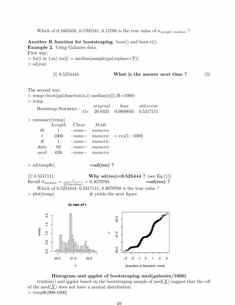
Which of 0.1605435, 0.1705241, 0.15708 is the true value of σsample median ?

Another R function for bootstraping: boot() and boot.ci().Example 2. Using Galaxies data.First way:> for(i in 1:m) res[i] = median(sample(gal,replace=T))> sd(res)

[1] 0.5254444 What is the answer next time ? (3)

The second way:> temp=boot(gal,function(x,i) median(x[i]),R=1000)> temp

Bootstrap Statistics :original bias std.error

t1∗ 20.8335 0.0808045 0.5317111

> summary(temp)Length Class Mode

t0 1 −none− numerict 1000 −none− numeric = res[1 : 1000]R 1 −none− numericdata 82 −none− numericseed 626 −none− numeric· · ·

> sd(temp$t) =sd(res) ?

[1] 0.5317111 Why sd(res)=0.525444 ? (see Eq.(1))Recall σmedian = 1

2f(median)= 0.4079768. =sd(res) ?

Which of 0.5254444, 0.5317111, 0.4079768 is the true value ?> plot(temp) # yields the next figure

Histogram of t

t*

Density

20.0 21.0 22.0

0.0

0.5

1.0

1.5

2.0

−3 −2 −1 0 1 2 3

20.0

21.0

22.0

Quantiles of Standard Normal

t*

Histogram and qqplot of bootstraping med(galaxies/1000)truehist() and qqplot based on the bootstraping sample of med(X) suggest that the cdf

of the med(X) does not have a normal distribution.> temp$t[998:1000]

49

[998,] 20.7120

[999,] 20.7950

[1000,] 21.8675

Confidence interval of a parameter (L,R):

e.g. 95% approximate CI of θ satisfies PL < θ < R ≈ 0.95.

If θ is approximately N(θ, σ2θ), then

(L,R) = (θ − 1.96σθ, θ + 1.96σθ),

as Pθ − θ > 1.96σθ ≈ 0.025.

θ may not be approximately normal, then there are several approaches:

(1) percentile CI, (2) basic CI and (3) bca.

(1) percentile CI: One expects that θ ≈ θ, the edf Fθ∗ of θ∗ ≈ the cdf of Fθ,

the empirical quantile Qθ∗(0.025) and Qθ∗(0.975) satisfies

PQθ∗(0.025) ≤ θ ≤ Qθ∗(0.975) ≈ 0.95,

thus

(L,R) = (Q(0.025), Q(0.975))

is called the percentile CI.L (R) is the 2.5th (97.5th) quantile of the edf of the m θ∗1 , ..., θ∗ms.(2) Basic CI: One expects that

0.95 = P (a ≤ θ − θ ≤ b) ≈ P (a ≤ θ∗ − θ ≤ b).

Thus a and b are the 2.5th and 97.5th quantiles of the edf based on θ∗i − θ, i = 1, ..., m.

A 95% CI is (L,R) ≈ (θ − b, θ − a). It can be shown that

(L,R) ≈ (2θ − Qθ∗(0.975), 2θ − Qθ∗(0.025)).

(3) bca. R also gives another CI denoted by bca or BCa (see BCa on page 136 of V&R).

Three program for bootstraping galaxies data:gal=galaxies/1000(1) m=1000; res=numeric(m) # res=rep(0,m)

for(i in 1:m) res[i] = median(sample(gal,replace=T))

s=sd(res) # sample SD of sample median

x=median(gal)

c(x-1.96*s,x+1.96*s) # normal CI

(y=quantile(res,p=c(0.025,0.975))) # percentile CI y=sort(res)[c(25,975)]

2*x-y[2:1] # ??(2) temp=boot(gal,function(x,i) median(x[i]),R=1000)

boot.ci(temp, type = c(”norm”, ”basic”, ”perc”, ”stud”))(3) fun = function(d, i)

m = median(d[i])

n = length(i)

v = (n-1)*var(d[i])/n**2 # var(x) = 1n−1

∑ni=1(xi − x)2

c(m, v)

temp=boot(gal,fun, R=1000)

boot.ci(temp, type = c(”norm”, ”basic”, ”perc”, ”stud”))

boot.ci(temp)

50

Output:

(1)> c(x-1.96*s,x+1.96*s)[1] 19.79584 21.87116> (y=quantile(res,p=c(0.025,0.975)))

2.5% 97.5%20.17245 22.05300

> 2*x-y[2:1]97.5% 2.5%

19.61400 21.49455(2)

> temp=boot(gal,function(x,i) median(x[i]),R=1000)> boot.ci(temp, type = c(”norm”, ”basic”, ”perc”, ”stud”))

BOOTSTRAP CONFIDENCE INTERVAL CALCULATIONSBased on 1000 bootstrap replicatesCALL :boot.ci(boot.out = temp, type = c(”norm”, ”basic”, ”perc”, ”stud”))Intervals :Level Normal Basic Percentile95% (19.78, 21.81) (19.62, 21.50) (20.17, 22.05)

(3)> boot.ci(temp, type = c(”norm”, ”basic”, ”perc”, ”stud”))

Intervals :Level Normal Basic95% (19.78, 21.81) (19.62, 21.50)Level Studentized Percentile95% (19.57, 21.59) (20.17, 22.05)

> boot.ci(temp)Intervals :Level Normal Basic Studentized95% (19.78, 21.81 ) (19.62, 21.50 ) (19.57, 21.59 )Level Percentile BCa95% (20.17, 22.05 ) (20.08, 21.92 )

§5.5. Robust estimators.Suppose that X1, ..., Xn are i.i.d. from a df f = f(·; θ), θ ∈ Θ ⊂ Rp.

θ =? (estimation of θ).Several methods:

1. MLE. θ = argmaxθ∏n

i=1 f(Xi; θ).

2. MME. Solution to Xk = Eθ(Xk), k = 1, ..., p.

3. MDE. θ = argminθ∑n

i=1 |Xi − θ|, or

θ = argminθ√∑n

i=1 |Xi − θ|2 = argminθ∑n

i=1(Xi − θ)2 (LSE).

4. Bayes estimator. θ = argminθr(π, θ) (r is the Bayes risk of θ),

π is a density function of θ, r(π, θ) = E(E((θ(X) − θ)2|θ))5. Robust estimator ?

Location or scale parameter example. Suppose Xi are from a cdf F with median m

51

or mean µ, and scale τ or standard deviation σ.Example 1. Exp(1) distribution. µX =1, median m =ln2 and σX =1.

The mean and median are both called location or center.The SD is called a scale.

Exp(θ) distribution. µX = θ, median m =ln2/θ and σX = θ.The mean and median are now called location parameters.σX is called a scale parameter.

Example 2. Cauchy Distribution f(x; θ, τ) = fo(x−θτ ), where fo(x) = 1

π(1+x2) .

θ is the median, a location parameter, the mean = ?τ is a scale parameter, the standard deviation = ?

If the distribution is symmetric about the center (e.g., N(µ, σ)),mean and median are the same (Is it correct ??)X and med(X) are two location estimators.

S =√

1n−1

∑ni=1(Xi −X)2 is a scale estimator.

Note that µ and median are often quite close.X 6= µ ! (estimate θ 6= θ !)

Example 3. (A simulation study on N( , ) and Exp()).> x=rnorm(10)> x=c(x,100)

The data x can be roughly viewed as a random sample from

FX(t) =1

11[1(t ≥ 100) + 10Φ(t)], where Φ(t) is the cdf of N(0, 1).

> mean(x) =E(X) ?[1] 9.138084 # compare to the mean of N(0,1)

> median(x) =mdef= median of X ?

[1] 0.1937377 # compare to the median of N(0,1)m= ? m < 100 or m≥100 ?0.5 = F (m) = 1

11 [0 + 10Φ(m)]> qnorm(.55) # median of X

[1] 0.1256613> 100/11 # E(X)

[1] 9.090909> x=rexp(40)> x=c(x,100)> mean(x)

[1] 3.254283 # compare to the mean of Exp(1)> median(x)

[1] 0.6262377 # compare to the median of Exp(1) i.e., log(2) ≈ 0.693In the above examples, 100 in x is called an outlier.Observation:

med(X) is less sensitive to outliers than X.X : 9.1 3.3 median(x) : 0.19 0.63

0 1 0 0.69Outliers distort some estimators greatly. In fact,

limX1→±∞

X = ±∞

limX1→±∞

med(X) is finite (=med(X2, ..., Xn)).

52

Q: How to quantify outliers ?Use boxplot for detecting outliers.

Example 4. Boxplots of data chem and abbey.> summary(chem) # (24 determinations of copper in wholemeal flour)

Min. 1st Qu. Median Mean 3rd Qu. Max.2.200 2.775 3.385 4.280 3.700 28.950

> summary(abbey) # (31 Daily Price Returns Of Abbey National Shares)Min. 1st Qu. Median Mean 3rd Qu. Max.5.20 8.00 11.00 16.01 15.00 125.00

> x=c(rnorm(40),10)> boxplot(x)> boxplot(chem, sub=”chem”)> boxplot(abbey, sub=”abbey”)

−2

02

46

810

510

15

20

25

30

chem

20

40

60

80

100

120

abbey

Def. If an observation is more than 4 IQR (inter-quartile-range or Q3 −Q1) away from thecenter of the data, it is called an outlier.

center —- median

lower and upper hinges —– 1st and 3rd quartiles

whiskers ———- 1.5 IQR from hinges (unless max or min < 1.5 IQR).

Observations outside whiskers are suspected outliers.

It is definitely an ourlier if it is

3 IQR away from hinges, or

3 SD away from the center.Outliers may due to typos, errors or maybe true observations.

The sample can be viewed as from X =

U if Y = 0V if Y = 1,

, or

FX(x; θ) = (1 − α)FU (x; θ) + αFV (x), α ∈ [0, ǫ), and Y ∼ bin(1, α).

Q: How to quantify that an estimator is less sensitive to outliers ?

Ans: Stability and resistancy.

Def. An estimator is stable if it does not change by a large amount when an outlier isadded in. In particular, the estimator is bounded no matter what the outlier is equal to.The breakdown value (or point) of an estimator is the supremum value of the proportionp of the sample that can be moved to ∞ without the statistic moving to ∞ (in the case thatthe sample size is as large as necessary).An estimator with a large breakdown point is said to be ”resistant (to gross errors)”.

Remark. Definition from “Robust Nonparametric Statistical Methods”

53

by T.P. Hettmansperger and J.W. Mckean (1998) is as follows:Asymptotic breakdown point.Let x = (x1, ..., xn) represent a realization of a sample andlet x(m) ∈ Rn represent the corruption of any m of the n observations, that is,

xi1 , ..., xin−m among x1, ..., xn are fixed at their original values,but the rest m observations are changing (possibly to ±∞).

Let X be the collection of all combination of choosing m xi’s among x1, ..., xn to be cor-rupted with the rest fixed. Of course, X depends on the sample and it contains sequences ofelements that ||x(m)|| tend to ∞. We define the bias of an estimator θ to be

bias(m; θ,x) = sup|θ(x(m)) − θ(x)| : x(m) ∈ X

If the bias is infinite, we say the estimator has broken down and the

sample breakdown value = minm/n : bias(m; θ,x) = ∞

Its limit as n→ ∞, if it exists, is called the (asymptotic) breakdown value,

p = breakdown value = limn→∞

minm/n : bias(m; θ,x) = ∞

For med(X), p=50%.e.g., if n is 5 and less than half of the sample are moved to +∞,

med(X) is bounded by original values of X(1) and X(n).However, if 3 observations are moved to +∞, med(X) → ∞.Thus the sample breakdown value of med(X) is 3/5 if n = 5,

and is

1+n/2

n if n is evenn+12n if n is odd.

The limit or the (population) breakdown value is thus p = 1/2.For X, p=0 (asymptotically), as the sample breakdown value is 1/n.Q: Robustness ?Def. Let θ ∈ R, the relative efficiency (RE) of θ to θ is

RE(θ, θ) = limn→∞(σθ/σθ) = limn→∞(σθ/σθ) a.e.,

where σ2θ

– estimator of the asymptotic variance of θ (limn→∞ σθ/

√

V ar(θ) = 1), ...

Under the exponential family, if θ is the MLE of θ ∈ Rp, then

nΣ2θ≈ (E(dlnf(X;θ)

dθdlnf(X;θ)

dθ′ ))−1 (as nΣ2θ

P→(E(dlnf(X;θ)dθ

dlnf(X;θ)dθ′ ))−1).

∑ni=1

dlnf(Xi;θ)dθ

dlnf(Xi;θ)dθ′ → nE(dlnf(X;θ)

dθdlnf(X;θ)

dθ′ ) a.s. ?Are they right ?

Σ2θ

= (∑n

i=1dlnf(Xi;θ)

dθdlnf(Xi;θ)

dθ′ )−1|θ=θ, and Σ2θ≈ (

∑ni=1

dlnf(Xi;θ)dθ

dlnf(Xi;θ)dθ′ )−1|θ=θ

σ2θ

= (∑n

i=1(dlnf(Xi;θ)dθ )2)−1|θ=θ ?

σ2θ

= (∑n

i=1−d2lnf(Xi;θ)

dθ2 )−1|θ=θ ?

ARE(θ, θ) — asymptotic RE of θ to θ.Robust method studies how to find a stable or resistant estimator θ

with a large ARE(θ, θ) to a (possibly efficient or standard) estimator θunder F (·; θ) = (1 − α)Fo(·; θ) + αF1.The resulting estimator is called a robust estimator.

It is often that the standard situation is under the normal assumption.

54

Example 1. If X has the density f(x) = fo(x− µ),

ARE(med(X),X) =

64% if fo is N(0, σ2)96% if fo is t5> 1 if fo = exp(−|x|)/2

(the standard double exponential distribution)They are all symmetric distributions and thus m = µ.

Homework. Prove or disprove the following two statements:1. f(x; θ) = 1(x ≥ θ)exp(−(x− θ)) belongs to the exponential family.2. The double exponential distribution f(x; θ) = e−|x−θ|/2 belongs to the exponential family.Q: What are the candidates of robust estimators ?A class of location estimators:

M-estimators (MLE-like estimators).Consider a location parameter related to f(x− µ), where

f(x) is a density with∫f(x)dx = 1.

The MLE of µ satifies:

µ =

argminµ(−ln

∏ni=1 f(Xi − µ))

zero.pointµ∑n

i=1(lnf(Xi − µ))′ if the zero point exists

µ =argminµ

n∑

i=1

ρ(Xi − µ) with ρ = −lnf (1)

µ =zero.pointµ

n∑

i=1

ψ(Xi − µ) with ψ = f ′(Xi−µ)f(Xi−µ) = ρ′ if the zero point exists

Examples of (ρ and ψ):

The MLE X under N(µ, σ2): ρ = x2/2 & ψ(x) = x.The MLE med(X) under the DE (double exponential) ρ = |x| & ψ(x) = sign(x)

(2)

DE: f(x) = 12τ e

−|x−µ|τ .

Remark: The MLE under N(µ, σ2) is X, which is not robust if X 6∼ N(µ, σ2).The MLE under the DE is med(X), which is robust even if X is no longer the DE.

But they motivate the MLE-like function ρ and the score function ψ (= ρ′).Now the ρ does not have to related to −lnf , and ψ does not need to related to −(lnf)′.

Example 1. med(X): ρ = |x| and ψ(x) = sign(x) (see Eq.s (1) and (2) above). That is,

med(X) = zero.pointµ

n∑

i=1

ψ(Xi − µ) = zero.pointm

n∑

i=1

sign(Xi −m)

zero.pointm∑n

i=1 sign(Xi −m) = ?? How to derive it ?If n = 4, Xi = i, Med(X)= (X(2) +X(3))/2 or ∈ (X(2), X(3)).

zero.pointµ∑n

i=1 ψ(Xi − µ) = (X(2) +X(3))/2, as

∑ni=1 sign(Xi −m)

> 0 if m < X(2)

= 0 if m ∈ [X(2), X(3)]< 0 if m > X(3)

Is it right ?

If n = 3, Med(X)= X(2) = zero.pointm∑n

i=1 sign(Xi −m), as

55

∑ni=1 sign(Xi −m)

> 0 if m < X(2)

= 0 if m = X(2)

< 0 if m > X(2)

Is it right ?

If n = 5, Xi’s are 1, 2, 2, 3, 4, Med(X)= ??zero.pointm

∑ni=1 sign(Xi −m) = ?? How to derive it ?

∑5i=1 sign(Xi −m)

≥ 3 if m < 2= 1 if m = 2= −1 if m ∈ (2, 3)< −1 if m ≥ 3

???

There is no solution in this case to zero.pointm∑n

i=1 sign(Xi −m)How to handle it ??Interprete zero.pointm

∑ni=1 sign(Xi −m) as

zero.crossing.point∑n

i=1 sign(Xi −m)

56

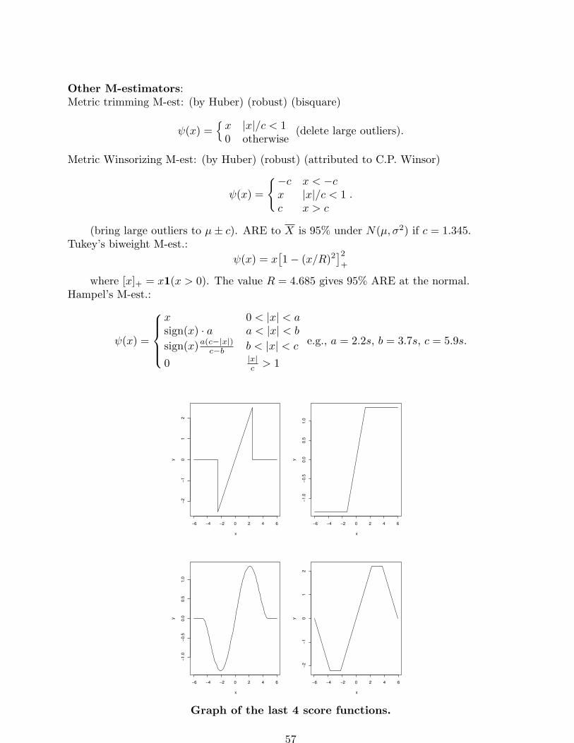
Other M-estimators:Metric trimming M-est: (by Huber) (robust) (bisquare)

ψ(x) =x |x|/c < 10 otherwise

(delete large outliers).

Metric Winsorizing M-est: (by Huber) (robust) (attributed to C.P. Winsor)

ψ(x) =

−c x < −cx |x|/c < 1c x > c

.

(bring large outliers to µ± c). ARE to X is 95% under N(µ, σ2) if c = 1.345.Tukey’s biweight M-est.:

ψ(x) = x[1 − (x/R)2

]2

+

where [x]+ = x1(x > 0). The value R = 4.685 gives 95% ARE at the normal.Hampel’s M-est.:

ψ(x) =

x 0 < |x| < asign(x) · a a < |x| < b

sign(x)a(c−|x|)c−b b < |x| < c

0 |x|c > 1

e.g., a = 2.2s, b = 3.7s, c = 5.9s.

−6 −4 −2 0 2 4 6

−2

−1

01

2

x

y

−6 −4 −2 0 2 4 6

−1

.0−

0.5

0.0

0.5

1.0

x

y

−6 −4 −2 0 2 4 6

−1

.0−

0.5

0.0

0.5

1.0

x

y

−6 −4 −2 0 2 4 6

−2

−1

01

2

x

y

Graph of the last 4 score functions.

57

Remark. There is scaling problem above (c, R and s are unknown).It can be replaced by an estimate of a scale parameter.

Possible estimators of scale parameter:

non-robust

S =√

1n−1

∑ni=1(Xi −X)2 (breakdown point p = 0).

σm = 1n

∑ni=1 |Xi −X|

√

π/2 (breakdown point p = 0)

robust

mad(X)=med(|X −med(X)|)/0.6745σq = IQR/1.35

The coefficients are made so that they equal σ under the normal distribution.huber(y, k = 1.5, tol = 1e-06)

Finds the Huber M-estimator of location with MAD scale.hubers(y, k = 1.5, mu, s, initmu = median(y), tol = 1e-06)

Finds the Huber M-estimator for location with scale specified,scale with location specified, or both if neither is specified.

mad(x, center = median(x), constant = 1.4826)> length(chem)[1] 24> x=sort(chem)> mean(x)[1] 4.280417> mean(x[2:23])[1] 3.253636> mean(chem,trim=0.05)[1] 3.253636> mean(chem,trim=0.1)[1] 3.205> median(x)[1] 3.385> median(x[2:23]) = ?> sd(chem)[1] 5.297396> mad(chem)[1] 0.526323> unlist(huber(chem))

mu s3.206724 0.526323

> huber(chem)$mu[1] 3.206724> unlist(hubers(chem))

mu s3.205498 0.673652

robust estimates

> fitdistr(chem,”t”,list(m=3,s=0.5),df=5)m s

3.1853947 0.6422023(0.1474804) (0.1279530)

MLE

> fitdistr(chem,”t”,df=5) # same results

58

§6.9. A Comment on the MLE with regression data.Let (X1, Y1), ..., (Xn, Yn) be i.i.d. observations from FX,Y ,

where X ∈ Rp, a column vector.The LSE

β = (XX ′ −X(X ′))−1(X ′Y −X ′(Y )). (1)

βa.s.→β∗ = Σ−1(E(X ′Y ) − E(X ′)E(Y )) (2)

if the expectations exist. This is due to ????Remark 1. Equations (1) and (2) do not rely on the assumption that (X,Y ) satisfies thelinear regression model:

Yi = X ′iβ + α+ ǫi

where ǫis are i.i.d. with E(ǫi|Xi) = 0 and σ2 = V ar(ǫi|Xi).It is often to further assume ǫi ⊥ Xi and/or ǫi ∼ N(0, σ2).

Remark 2. Y = βX + α+ ǫ<=> Y − βX − α = ǫ and fY |X(t|x) = fǫ(t− α− βx

︸︷︷︸

u

).

<=> Y − βX = W and fY |X(t|x) = fW (t− βx). W = ??

Example 1. If Y |(X = x) ∼ N(βx+ α, σ2), then W ∼ N(α, σ2). Y = βX + α+ ǫ.

Example 2. If Y = βX +W , W ∼ Exp(1), then

fY |X(t|x) = fW (t− βx) = e−(t−βx), t >??

Does Y |X have an Exponential distribution ?

Remark 3. lnY = βX + α+ ǫ,<=> Y = eβXW<=> fY |X(t|x) = fW ( t

eβx ) (= fW (w)), and lnW = α+ ǫ.

Example 3. If SY |X(t|x) = exp(−e−βxt) = SW (t/eβx), t > 0, then W ∼ ?Y |(X = x) ∼ ??

Y = W/eβX ? or Y = W/e−βX ?lnY = βX + α+ ǫ ? or lnY = −βX + α+ ǫ ?

Remark 4. If Y = βX + α+ ǫ, then the LSEα = Y − βX, where β is as in Eq. (1). Or the simpler formula:

(α, β′)′ = (B′B)−1B′Y, where B =

1 X ′i

......

1 X ′n

= (1,X)n×(1+p) and Y = (Y1, ..., Yn)′.

The LSE satisfies E(β) = β and V (α, β′|X) = σ2(B′B)−1.If ǫ 6∼ N(0, σ2), then the anova table is not valid as it is based on F distribution; and

the LSE is not an efficient estimator.One can also consider regression models under the parametric assumption.Assume that Yi|(Xi = x) ∼ F , where F = Fo(y|x, β) has a parametric form,

and Fo is known except β.

59

Then in order to find F , it suffices to find β.A standard estimator is the MLE, that maximizes

L(b) =∏n

i=1 fo(Yi|Xi, b),where fo is the density of Fo and So = 1 − Fo.

The MLE is efficient if the parametric assumption is valid and certain regularity con-ditions are satisfied.1. Gaussian distribution

Common form f(t) = 1√2πσ2

exp(− (t−µ)2

2σ2 ), t > 0

With covariate in Splus or R, reparametrization:

fY (y|x, β) = 1√2πσ2

exp(− (y−β′x)2

2σ2 )

or Y = β′x + σZ, Z ∼ N(0, 1). E(Z) = 0 ???2. Exponential distribution

Common form S(t) = exp(−t/θ), t > 0.With covariate in Splus or R, reparametrization:SY (y|x, β) = exp(−e−β′xy), y > 0. E(Y |x, β) = eβx.lnY = β′x + lnZ, Z ∼ Exp(1). E(lnZ) = 0 ???E(lnZ) =

∫· · · ??

E(ln(Z)) ≈ −0.585.3. Weibull distribution

Common form S(t) = exp(−tγ/θ), t > 0.With covariate in Splus or R, reparametrization:SY (y|x, β) = exp(−e−β′x/τy1/τ ), y > 0.lnY = β′x + τ lnZ, Z ∼ Exp(1). E(τ lnZ) = 0 ???Z = (e−β′xY )1/τ .That is, S(t) = exp(−(t/µ)1/τ ), t > 0. (S(t) = exp(−tγ/θ), t > 0).

4. Logistic distributionCommon form S(t) = 1

1+exp(t) ,

With covariate in Splus or R, reparametrization:SY (y|x, β) = 1

1+exp( y−β′xτ )

,

Y = β′x + τZ, Z ∼ logistic(0, 1). E(Z) = 0, σZ = π/√

3.5. Lognormal distribution

Assume lnY = β′x + σZ, where Z ∼ N(0, 1). E(Z) = 0 ???6. Loglogistic distribution

lnY = β′x + τZ, Z ∼ logistic(0, 1). E(Z) = 0 ???Remark. About lnY = βX + Z. If fY |X(t|x) = e−βxfo(te−βx), where fo is a df.

Then U = eZ = Y/eβx has d.f. fo.This is due to u-substitution.

∫ y

−∞e−βxfo(t/eβx)dt =

∫ y/eβx

−∞fo(u)du, where u = t/eβx.

R command:The parametric MLE is efficient under certain regularity assumptions. In particular,

if the residual plot suggests that certain parametric family is plausible,one can apply the R functions as follows.

zz=survreg(Surv(y)∼x, dist=”exponential”)

60

dist: (default: weibull), gaussian, logistic, lognormal and loglogisticglm()

The generalized linear model includes a subset of the exponential family, which is also para-metric distributions. The conditional distribution fY |X may not satisfy the linear regressionmodel or log linear regression model. We can compute the MLE of the parameters basedon regression data. The GLM includes

N(µ, σ2),G(α, β),bin(m, p)Poisson(µ)inverse-GaussianWe only review G(α, β) here.The gamma distribution family belongs to the generalized linear model (glm) but does

not satisfy the ordinary linear regression model or the ordinary log linear regression model.7. Gamma Distribution. fY (y) = 1

Γ(α)βα yα−1e−y/β , y, α, β > 0.

If α 6= 1, then treat α as known. Thus µ = αβ, it can be shown that

lnfY (y) = α︸︷︷︸Aiφ

[y (−1/µ)︸︷︷︸

θi

− lnµ︸︷︷︸

γ(θi)

] + [αlnα− lnΓ(α) + (α− 1)lny]︸︷︷︸

τ(y,Aiφ )

(the form of the generalized linear model).Then θi = −1

µi,

Ai/φ = α,γ(θi) = −ln(−θi).

The link l(µi) = β′Xi and µi = l−1(β′Xi).The default link is l(µi) = −1/µi = β′Xi. µi = −1/(β′Xi)The other links are l(µ) = µ and ln(µ),The identity leads to µi = β′Xi.=> Y = β′X +W , E(Y |X) = β′X ?

V (Y |X) = (β′X)2

α ?The log leads to µi = exp(β′Xi)=> lnY = β′X +W , E(Y |X) = eβ

′X ?E(lnY |X) = β′X ??inverse leads to µi = −1/(β′Xi).

lnfY |X(y|xi) =

α︸︷︷︸Aiφ

[y (−1/µ)︸︷︷︸

βxi

− lnµ︸︷︷︸

ln( −1βxi

)

] + [αlnα− lnΓ(α) + (α− 1)lny]︸︷︷︸

τ(y,Aiφ )

inverse link

α︸︷︷︸Aiφ

[y (−1/µ)︸︷︷︸

−1/βxi

− lnµ︸︷︷︸

ln(βxi)

] + [αlnα− lnΓ(α) + (α− 1)lny]︸︷︷︸

τ(y,Aiφ )

identity link

α︸︷︷︸Aiφ

[y (−1/µ)︸︷︷︸

−1/eβxi

− lnµ︸︷︷︸

ln(eβxi )

] + [αlnα− lnΓ(α) + (α− 1)lny]︸︷︷︸

τ(y,Aiφ )

log link

Example 1. Carry out a simulation study on the LSE and MLE of β (β = 2), under theassumption that conditional on X = x,

lnY = 2x+ lnZ orY = eβxZ, where Z ∼ Exp(1).

61

library(MASS); library(survival);n=500x=sample(1:4,n,replace=T)b=2y=rgamma(n,1,exp(-b*x))# y=rexp(n,scale=exp(b*x))# y=rweibull(n,1,exp(-b*x))z=lm(log(y)∼x)z=survreg(Surv(y)∼x) #weibullz=glm(y∼x,family=Gamma(link=log),maxit=50)z=survreg(Surv(y)∼x, dist=”exponential”)z=survreg(Surv(y)∼x-1, dist=”exponential”)z=lm(log(y)∼x-1)summary(z) # for each of the 6 zpredict(z,data.frame(x=4),se=T) # estimate E(Y |X = 4) with SE

V alue Std. Error z pexp(α+ βx) ∼ x

LSE(Intercept) −0.59293 0.15615 −3.797 0.000164

x 1.96718 0.05792 33.964 < 2e− 16survreg(weib)

(Intercept) 0.0591 0.1219 0.485 0.628x 1.9563 0.0449 43.530 0.000

Log(scale) 0.0721 0.0351 2.053 0.040glm(gamma)

(Intercept) 0.09658 0.11475 0.842 0.4x 1.95446 0.04256 45.920 < 2e− 16

survreg(exp)(Intercept) 0.0966 0.1123 0.86 0.39

x 1.9545 0.0419 46.66 0.00

exp(βx) ∼ x− 1survreg(exp)

x 1.99 0.0168 119 0LSE

x 1.76649 0.02401 73.57 < 2e− 16

Remark. One can find some interesting facts from the table.

1. Notice that α

≈ 0 in the MLE of exp(α+ βx) or Weibull,≈ −0.59 for the LSE (Anything wrong ?)

2. Relation between the σ oflm(y ∼ x), Gamma y ∼ x, Weibull y ∼ x, Exp y ∼ x and Exp y ∼ x− 1.Which is smaller ?

Why such a relation ?Which estimator of β is better ?

Answer to question in (1):α = 0 in the MLE approach under Exp(eβx), butα = E(ln(Z)) ≈ −0.585 in the LSE approach lnY = βX + lnZ = βX + α+ ǫ.

62

Answer to question in (2):(a) Semi-parametric v.s. parametric approach;(b) The # of parameters go from 4 to 1.

Simulation Example 2. About ∼ 1 v.s. ∼ x or ∼ x− 1.Let Y ∼ Exp(µ).S(t) = exp(−λt)1(t > 0), λ = 1/µ.

= exp(− tµ )1(t > 0,

Z = Yµ , where Z ∼ Exp(1).

lnY = lnµ+ lnZ.y=rexp(500)fitdistr(y,”exponential”)survreg(Surv(y)∼ 1, dist=”exponential”)glm(y∼1,family=Gamma(link=log))lm(log(y)∼1)

Question: What is the true value that is estimated ?How many distinct values of the estimates ?method estimatefitdistr 1.047001 rate

1/Y 1.047001 Are these 2 always the same ?survreg −0.04593031logY −0.04593031glm() −0.04593 Are these 3 always the same ?

lm(lnY ∼ 1) −0.5651lnY −0.5650986 Are these two the same ?

Suppose Y ∼ Exp(µ) where E(Y ) = µ.The MLE of E(Y ) is Y .

method estimateY 0.9551085 µ

fitdistr 1.047001 λ S(t) = exp(−λt) = exp(−t/µ)1/Y 1.047001 1/µ

survreg −0.04593031 −ln(λ) lnY = logµ+ lnZlogY −0.04593031 log µ

glm() −0.04593 ˜lnµlm(lnY ∼ 1) −0.5651 α for lnY = α+ ǫ α = E(lnZ) ≈ −0.58

lnY −0.5650986 α ≈ −0.58 + 0.01490145

Remark. In both the MLE approach and the LSE approach,the SE is derived through the approximation (delta method or Slutsky’s theorem).

If g(·) has continuous gradient and Xi’s are i.i.d. with mean µ and covariance matrix Σ,then

nCov(g(X)) ≈ ∂g

∂µ′Cov(X)∂g

∂µ

which can be further estimated by the consistent estimates of the unknown parameters.

63

From simulation example 1, we can see that the MLE of β is better than the LSE.How to check whether a parametric family fit the regression data ?Ans: There are two appoaches: (1) diagnostic plots: (2) testing.Diagnostic plots

1. Use qqplot of residuals against the quantiles of Fǫ(·; θ), where Y = βX + ǫ.2. Use the marginal distribution plots (MD plots): plot FY ∗ and the CB of FY , where

FY ∗ is the edf based on data generated from the Y ∗ satisfying the model with parameterestimated by the MLE.Model testing:

1. One sample ks.test,2. Two sample ks.test,3. MD test.

Example 3. Estimate E(Y |X = 4) based on the regression data of 100 pairs of (x,y)(given).> n=length(y)> ss=lm(y∼ x)> summary(ss)

Coefficients:Estimate Std.Error tvalue Pr(> |t|)

(Intercept) −1154.0 320.0 −3.606 0.000492 ∗ ∗ ∗x 728.4 115.4 6.312 8.05e− 09 ∗ ∗ ∗

Multiple R-squared: 0.289, Adjusted R-squared: 0.2818Diagnostic Plots.> plot(x,y)> plot(x,log(y)) (see Figure 1 below)

1.0 1.5 2.0 2.5 3.0 3.5 4.0

02

00

04

00

06

00

08

00

01

00

00

x

y

1.0 1.5 2.0 2.5 3.0 3.5 4.0

02

46

8

x

log(

y)

Figure 1. Qqplot of data (x,y)

64

> z=resid(ss)> qqplot(z,qexp((1:n)/(n+1))) # qqplot(1,1)> qqnorm(z) # qqplot(1,2)> tt=lm(log(y)∼ x)> z=resid(tt)> zz=survreg(Surv(y)∼ x)> qqplot(z,qexp((1:n)/(n+1))) # qqplot(2,1)# qqplot(z,log(qexp((1:n)/(n+1))))> qqplot(exp(z),qexp((1:n)/(n+1))) # qqplot(2,2)> qqplot(exp(z),qexp((1:n)/(n+1),1/mean(exp(z)))) # qqplot(3,1)

65

−2000 0 2000 4000 6000 8000

01

23

4

z

qexp((

1:n

)/(n

+ 1

))

−2 −1 0 1 2

−2000

4000

Normal Q−Q Plot


Sam

ple

Quantile

s−3 −2 −1 0 1 2

01

23

4

z

qexp((

1:n

)/(n

+ 1

))

−2 −1 0 1 2

−3

−1

1

Normal Q−Q Plot


Sam

ple

Quantile

s

−3 −2 −1 0 1 2

01

23

4

z

qexp((

1:n

)/(n

+ 1

))

−3 −2 −1 0 1 2

−4

−2

0

z

log(

qexp((

1:n

)/(n

+ 1

)))

0 2 4 6 8

01

23

4

exp(z)

qexp((

1:n

)/(n

+ 1

))

0 2 4 6 8

02

46

exp(z)qexp((

1:n

)/(n

+ 1

), 1

/mean(e

xp(z

)))

Left qqplots Right qqplots modelǫ ∼ Exp(1) ǫ ∼ N(0, σ2) Y = α+ βX + ǫ

lnZ ∼ Exp(1) Z = exp(logZ) ∼ Exp(1) log Y = α+ βX + logZZ ∼ Exp(µ) Y = eα+βXZ

ǫ ∼ N(0, σ2) Y = α+ βX + ǫZ ∼ Exp(1) Z = exp(logZ) ∼Weibull log Y = α+ βX + τ logZFigure 1. QQ-plots in Examples 3 & 4

Can we test it ?

66

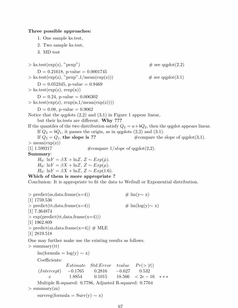
Three possible approaches:

1. One sample ks.test,

2. Two sample ks.test,

3. MD test

> ks.test(exp(z), ”pexp”) # see qqplot(2.2)

D = 0.21618, p-value = 0.0001745> ks.test(exp(z), ”pexp”,1/mean(exp(z))) # see qqplot(3.1)

D = 0.052345, p-value = 0.9469> ks.test(exp(z), rexp(n))

D = 0.24, p-value = 0.006302> ks.test(exp(z), rexp(n,1/mean(exp(z))))

D = 0.08, p-value = 0.9062Notice that the qqplots (2,2) and (3,1) in Figure 1 appear linear,

but their ks.tests are different. Why ???If the quantiles of the two distribution satisfy Q2 = a+bQ2, then the qqplot appears linear.

If Q2 = bQ1, it passes the origin, as in qqplots (2,2) and (3.1).If Q2 = Q1, the slope is ?? #compare the slope of qqplot(3,1).

> mean(exp(z))[1] 1.599217 #compare 1/slope of qqplot(2,2).Summary:

H0: lnY = βX + lnZ, Z ∼ Exp(µ).H0: lnY = βX + lnZ, Z ∼ Exp(µ).H0: lnY = βX + lnZ, Z ∼ Exp(1.6).

Which of them is more appropriate ?Conclusion: It is appropriate to fit the data to Weibull or Exponential distribution.

> predict(ss,data.frame(x=4)) # lm(y∼ x)[1] 1759.536> predict(tt,data.frame(x=4)) # lm(log(y)∼ x)[1] 7.364874> exp(predict(tt,data.frame(x=4)))[1] 1962.809> predict(zz,data.frame(x=4)) # MLE[1] 2819.518

One may further make use the existing results as follows.> summary(tt)

lm(formula = log(y) ∼ x)

Coefficients:Estimate Std.Error tvalue Pr(> |t|)

(Intercept) −0.1765 0.2816 −0.627 0.532x 1.8854 0.1015 18.566 < 2e− 16 ∗ ∗ ∗

Multiple R-squared: 0.7786, Adjusted R-squared: 0.7764> summary(zz)

survreg(formula = Surv(y) ∼ x)

67

V alue Std.Error z p(Intercept) 0.214 0.2458 0.872 3.83e− 01

x 1.932 0.0898 21.528 8.49e− 103Log(scale) −0.115 0.0784 −1.461 1.44e− 01

Scale= 0.892Weibull distribution

Question: What can be concluded from the last 2 summaries ?Questions: α = 0 or β = 2 or scale=1 ??> exp(4*2) # (= E(Y |X = 4), as Y = eβXZ, Z ∼ Exp(1)).[1] 2980.958 # Final answer to E(Y |X = 4).One may also construct a CI for E(Y |X = 4) through information in summary(zz).# exp(4*(2+1.96*tt$coef[2,2]*c(-1,1)))> u=predict(zz,data.frame(x=4),se=T)> c(u$fit-2*u$se.fit ,u$fit+2*u$se.fit) # based on MLE

(1906.055, 3732.980) # it contains 2981.> u=predict(tt,data.frame(x=4),se=T)> c(u$fit-2*u$se.fit ,u$fit+2*u$se.fit) # Which of the two is appropriate here> exp(c(u$fit-2*u$se.fit ,u$fit+2*u$se.fit)) # for prediction of Y ?

# based on LSE of lnY = βX + α+ ǫ.(1092.792, 2283.027 ) # Why doesn’t it contain 2981 ?

> u=predict(ss,data.frame(x=4),se=T)> u$fit+(2*u$se.fit*c(-1,1))

# based on LSE of Y + βX + α+ ǫ.( 1340.891 2178.180) # Why doesn’t it contain 2981 ?

Example 4.> n=100> x=sample(1:4,n,replace=T)> b=2> y=rweibull(n,scale=exp(b*x),shape=5)> zz=lm(y∼ x)> summary(zz)

lm(formula = y ∼ x)Coefficients:

Estimate Std.Error tvalue Pr(> |t|)(Intercept) −1335.26 152.38 −8.763 5.84e− 14 ∗ ∗ ∗

x 877.70 57.35 15.304 < 2e− 16 ∗ ∗ ∗> z=resid(zz)> qqnorm(z)

68

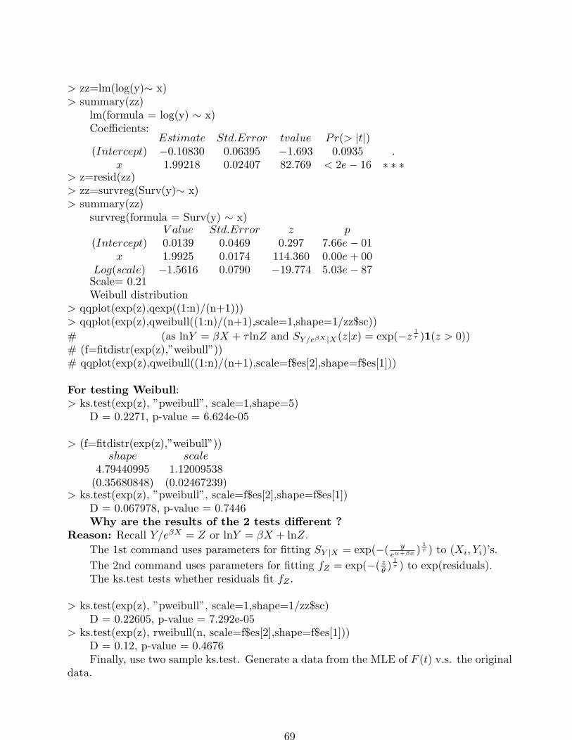
> zz=lm(log(y)∼ x)> summary(zz)

lm(formula = log(y) ∼ x)Coefficients:

Estimate Std.Error tvalue Pr(> |t|)(Intercept) −0.10830 0.06395 −1.693 0.0935 .

x 1.99218 0.02407 82.769 < 2e− 16 ∗ ∗ ∗> z=resid(zz)> zz=survreg(Surv(y)∼ x)> summary(zz)

survreg(formula = Surv(y) ∼ x)V alue Std.Error z p

(Intercept) 0.0139 0.0469 0.297 7.66e− 01x 1.9925 0.0174 114.360 0.00e+ 00

Log(scale) −1.5616 0.0790 −19.774 5.03e− 87Scale= 0.21Weibull distribution

> qqplot(exp(z),qexp((1:n)/(n+1)))> qqplot(exp(z),qweibull((1:n)/(n+1),scale=1,shape=1/zz$sc))

# (as lnY = βX + τ lnZ and SY/eβX |X(z|x) = exp(−z 1τ )1(z > 0))

# (f=fitdistr(exp(z),”weibull”))# qqplot(exp(z),qweibull((1:n)/(n+1),scale=f$es[2],shape=f$es[1]))

For testing Weibull:> ks.test(exp(z), ”pweibull”, scale=1,shape=5)

D = 0.2271, p-value = 6.624e-05

> (f=fitdistr(exp(z),”weibull”))shape scale

4.79440995 1.12009538(0.35680848) (0.02467239)

> ks.test(exp(z), ”pweibull”, scale=f$es[2],shape=f$es[1])D = 0.067978, p-value = 0.7446Why are the results of the 2 tests different ?

Reason: Recall Y/eβX = Z or lnY = βX + lnZ.

The 1st command uses parameters for fitting SY |X = exp(−( yeα+βx )

1τ ) to (Xi, Yi)’s.

The 2nd command uses parameters for fitting fZ = exp(−( zθ )

1τ ) to exp(residuals).

The ks.test tests whether residuals fit fZ .

> ks.test(exp(z), ”pweibull”, scale=1,shape=1/zz$sc)D = 0.22605, p-value = 7.292e-05

> ks.test(exp(z), rweibull(n, scale=f$es[2],shape=f$es[1]))D = 0.12, p-value = 0.4676Finally, use two sample ks.test. Generate a data from the MLE of F (t) v.s. the original

data.

69

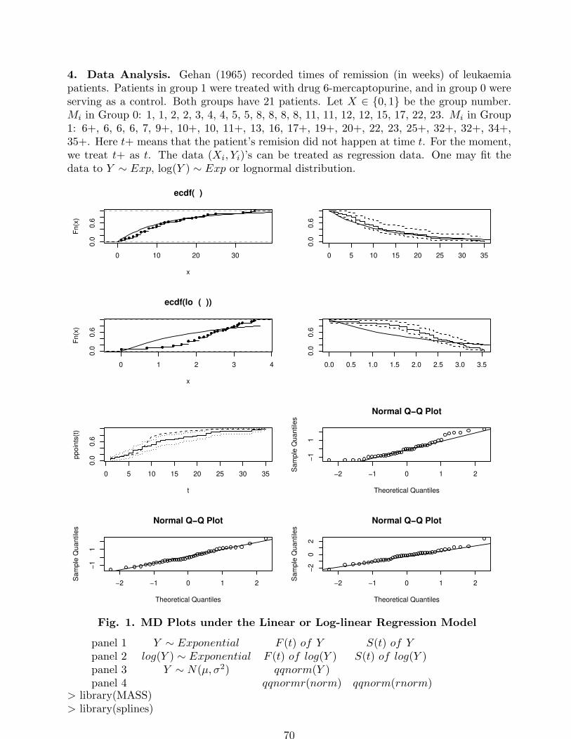
4. Data Analysis. Gehan (1965) recorded times of remission (in weeks) of leukaemiapatients. Patients in group 1 were treated with drug 6-mercaptopurine, and in group 0 wereserving as a control. Both groups have 21 patients. Let X ∈ 0, 1 be the group number.Mi in Group 0: 1, 1, 2, 2, 3, 4, 4, 5, 5, 8, 8, 8, 8, 11, 11, 12, 12, 15, 17, 22, 23. Mi in Group1: 6+, 6, 6, 6, 7, 9+, 10+, 10, 11+, 13, 16, 17+, 19+, 20+, 22, 23, 25+, 32+, 32+, 34+,35+. Here t+ means that the patient’s remision did not happen at time t. For the moment,we treat t+ as t. The data (Xi, Yi)’s can be treated as regression data. One may fit thedata to Y ∼ Exp, log(Y ) ∼ Exp or lognormal distribution.

0 10 20 30

0.0

0.6

ecdf(y )

x

Fn

(x)

0 5 10 15 20 25 30 35

0.0

0.6

0 1 2 3 4

0.0

0.6

ecdf(log (y ))

x

Fn

(x)

0.0 0.5 1.0 1.5 2.0 2.5 3.0 3.5

0.0

0.6

0 5 10 15 20 25 30 35

0.0

0.6

t

pp

oin

ts(t

)

−2 −1 0 1 2

−1

1

Normal Q−Q Plot


Sa

mp

le Q

ua

ntile

s

−2 −1 0 1 2

−1

1

Normal Q−Q Plot


Sa

mp

le Q

ua

ntile

s

−2 −1 0 1 2

−2

02

Normal Q−Q Plot


Sa

mp

le Q

ua

ntile

s

Fig. 1. MD Plots under the Linear or Log-linear Regression Model

panel 1 Y ∼ Exponential F (t) of Y S(t) of Ypanel 2 log(Y ) ∼ Exponential F (t) of log(Y ) S(t) of log(Y )panel 3 Y ∼ N(µ, σ2) qqnorm(Y )panel 4 qqnormr(norm) qqnorm(rnorm)

> library(MASS)> library(splines)

70

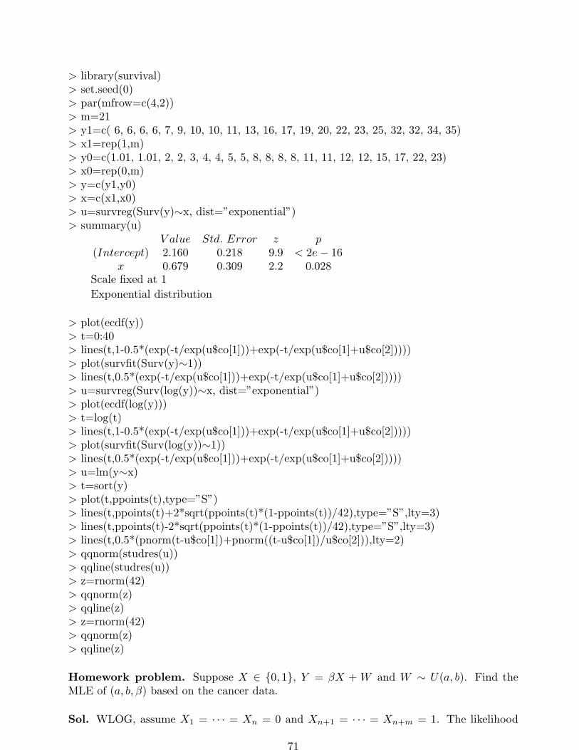
> library(survival)> set.seed(0)> par(mfrow=c(4,2))> m=21> y1=c( 6, 6, 6, 6, 7, 9, 10, 10, 11, 13, 16, 17, 19, 20, 22, 23, 25, 32, 32, 34, 35)> x1=rep(1,m)> y0=c(1.01, 1.01, 2, 2, 3, 4, 4, 5, 5, 8, 8, 8, 8, 11, 11, 12, 12, 15, 17, 22, 23)> x0=rep(0,m)> y=c(y1,y0)> x=c(x1,x0)> u=survreg(Surv(y)∼x, dist=”exponential”)> summary(u)

V alue Std. Error z p(Intercept) 2.160 0.218 9.9 < 2e− 16

x 0.679 0.309 2.2 0.028Scale fixed at 1

Exponential distribution

> plot(ecdf(y))> t=0:40> lines(t,1-0.5*(exp(-t/exp(u$co[1]))+exp(-t/exp(u$co[1]+u$co[2]))))> plot(survfit(Surv(y)∼1))> lines(t,0.5*(exp(-t/exp(u$co[1]))+exp(-t/exp(u$co[1]+u$co[2]))))> u=survreg(Surv(log(y))∼x, dist=”exponential”)> plot(ecdf(log(y)))> t=log(t)> lines(t,1-0.5*(exp(-t/exp(u$co[1]))+exp(-t/exp(u$co[1]+u$co[2]))))> plot(survfit(Surv(log(y))∼1))> lines(t,0.5*(exp(-t/exp(u$co[1]))+exp(-t/exp(u$co[1]+u$co[2]))))> u=lm(y∼x)> t=sort(y)> plot(t,ppoints(t),type=”S”)> lines(t,ppoints(t)+2*sqrt(ppoints(t)*(1-ppoints(t))/42),type=”S”,lty=3)> lines(t,ppoints(t)-2*sqrt(ppoints(t)*(1-ppoints(t))/42),type=”S”,lty=3)> lines(t,0.5*(pnorm(t-u$co[1])+pnorm((t-u$co[1])/u$co[2])),lty=2)> qqnorm(studres(u))> qqline(studres(u))> z=rnorm(42)> qqnorm(z)> qqline(z)> z=rnorm(42)> qqnorm(z)> qqline(z)

Homework problem. Suppose X ∈ 0, 1, Y = βX + W and W ∼ U(a, b). Find theMLE of (a, b, β) based on the cancer data.

Sol. WLOG, assume X1 = · · · = Xn = 0 and Xn+1 = · · · = Xn+m = 1. The likelihood

71

function is L(a, b, β) = (b− a)−n∏n

i=1[1(Xi = 0, Yi ∈ [a, b]) + 1(Xi = 1, Yi − β) ∈ [a, b])].Let Y(1|0) = minYi : i ∈ 1, ..., n,Y(n|0) = maxYi : i ∈ 1, ..., n,Y(1|1) = minYi+n : i ∈ 1, ...,m andY(m|1) = maxYi+n : i ∈ 1, ...,m.Then either (1) Yn|0 − Y1|0 ≤ Ym|1 − Y1|1 or (2) Yn|0 − Y1|0 > Ym|1 − Y1|1.In Case (1), if β is fixed, then the MLE of (a, b) is

(a, b) =

(Y(1|0), Y(m|1) − β) if Y(1|1) − β > Y(1|0)(Y(1|1) − β, Y(m|1) − β) if Y(1|1) − β ≤ Y(1|0) and Y(m|1) − β ≥ Y(n|0)(Y(1|1) − β, Y(n|0)) if Y(m|1) − β < Y(n|0)

=

(Y(1|0), Y(m|1) − β) if Y(1|1) − Y(1|0) > β(Y(1|1) − β, Y(m|1) − β) if Y(1|1) − Y(1|0) ≤ β ≤ Y(m|1) − Y(n|0)(Y(1|1) − β, Y(n|0)) if β > Y(m|1) − Y(n|0)

b− a =

Y(m|1) − Y(1|0) − β ≥ Y(m|1) − Y(1|1) if Y(1|1) − Y(1|0) > βY(m|1) − Y(1|1) if Y(1|1) − Y(1|0) ≤ β ≤ Y(m|1) − Y(n|0)Y(n|0) − Y(1|1) + β ≥ Y(m|1) − Y(1|1) if β > Y(m|1) − Y(n|0)

Thus the MLE is (a, b, β) = (Y(1|1)−β, Y(m|1)−β, β) where β ∈ [Y(1|1)−Y(1|0), Y(m|1)−Y(n|0)].In particular, we can choose β = [Y(1|1) − Y(1|0) + Y(m|1) − Y(n|0)]/2. Since Y(1|1) → a + β

a.s. and Y(m|1) → b+ β a.s., (a, b) → (a, b) a.s. in Case (1). Moreover, since Y(1|0) → a a.s.

and Y(n|0) → b a.s., (β) → β a.s. in Case (1).On the other hand, in Case (2), if β is given then the MLE is

(a, b) =

(Y(1|1) − β, Y(n|0)) if Y(1|1) − β < Y(1|0)(Y(1|0), Y(n|0)) if Y(1|1) − β ≥ Y(1|0) and Y(m|1) − β ≤ Y(n|0)(Y(1|0), Y(m|1) − β) if Y(m|1) − β > Y(n|0)

min(b− a) =Y(n|0) − Y(1|0) if Y(1|1) − Y(1|0) ≥ β ≥ Y(m|1) − Y(n|0)

Thus an MLE is (a, b, β) = (Y(1|0), Y(n|0), (Y(1|1) − Y(1|0) + Y(m|1) − Y(n|0))/2). Moreover, it

is easy to show (a, b, β) is consistent in Case (2).Remark. The Newton Raphson method may not work, as the derivative ∂L

∂β does not exist

at β ∈ Y(1|1) − Y(1|0), Y(m|1) − Y(n|0).————- Thenb ≥ 35 − β, b ≥ 23, a ≤ 1 and a ≤ 6 − β.If b ≥ 35 − β ≥ 23, a ≤ 1 ≤ 6 − β, then b− a ≥ 34 − β; = 29 => β = 5If b ≥ 35 − β ≥ 23, a ≤ 6 − β ≤ 1, then b− a ≥ 29;If b ≥ 23 ≥ 35 − β, a ≤ 1 ≤ 6 − β, then b− a ≥ 22;If b ≥ 23 ≥ 35 − β, a ≤ 6 − β ≤ 1, then b− a ≥ 17 + β. = 29 => β = 12Notice that L = 0 if b− a < max22, 29 and L decreases in b− a if b− a ≥ 29. Thus

b− a = 29. β ∈ [5, 12].If a = 1 and b = 30, then y0 ⊂ [1, 23] ⊂ [1, 30]; y1− β ⊂ [6− β, 35− β] ⊂ [1, 30] ? That

is, 1 ≤ 6 − β and 35 − β ≤ 30.β ≤ 5. Thus the solution is not unique. If one let β be the mean difference of E(Y |X)

for X = 0 and X = 1.Notice that Yi − βXi ∼ U(a, b). If β is fixed, then the MLE of (a,b) is

72

(1, 35 − β) if 6 − β ≥ 1(6 − β, 35 − β) if 6 − β < 1 and 23 < 35 − β(6 − β, 23) if 23 ≥ 35 − β

=

(1, 35 − β) if β ≤ 5(6 − β, 35 − β) if 5 < β < 12(6 − β, 23) if β ≥ 12

Appendix. The marginal distribution (MD) approach. Notice that existing modelchecking tests for testing

H0: Y = βX +W and X ⊥W v.s. Ho1 : H0 is false, (1.1)

such as residuals qqplot, ks.test the residuals, the F-test and t-test tests, are valid if(1) Y = βX + θg(X) + ǫ is true,(2) X ⊥ ǫ,(3) ǫ ∼ N(0, σ2).If (1) or (3) fails, the existing tests are not valid, and can be worse than random

guessing, let alone being consistent. Of course, if no better choice, something is better thanno choice.

We shall introduce a new approach for model checking, which is always consistent (insome sense to be introduced next) for testing H0: Y = βX + W and X ⊥ W v.s. Ho

1 : H0

is false.A.1. Preliminary. We assume that

(X1, Y1), ..., (Xn, Yn) are i.i.d. observations from Fx,Y , with density function fx,Y ,where X is a p-dimensional random vector and Y is a response variable.Let FY |x be the conditional cdf with density function fY |x.Denote Fo = FY |x(·|0), which is called the baseline cdf of FY |x. The LR model is oftenformulated by

Y = β′X + α+ ǫ, where E(ǫ|X) = 0. (1.2)

If the conditional variance V ar(W |X) does not depend on X, it is called an ordinary linearregression (OLR) model, otherwise, it is called a weighted linear regression (WLR) model.Remark 1. Advantages that the LR model is specified by Eq. (1.1) rather than (1.2) are:(1) Eq. (1.2) but not (1.1) requires that E(Y |X) exists;(2) In general, β but not α is identifiable under censorship models (Yu and Wong (2002));(3) It is often less important to estimate α than β, the effect of the covariate X on Y .Under the OLR model, there are several consistent estimators of β if Fx,Y ∈ Θlse, where

Θlse = Fx,Y : Σx is non-singular and Cov(X, Y ) exists, (1.3)

and Σx is the p× p covariance matrix of X. They includethe semi-parametric MLE (SMLE) (if Fo is discontinuous),the modified SMLE (MSMLE) (see Yu and Wong (2002, 2003 and 2004)),the least squares estimator (LSE) andthe quantile or median regression estimator.

Yu and Wong (2002) show thatthe MSMLE is still consistent if E(lnfW (W )) exists, andthe MSMLE (or SMLE) β satisfy P (β 6= β infinitely often) = 0 if the cdf FW isn’t cts.However, the LSE is inconsistent if E(|Y ||X) = ∞.Given Fx,Y ∈ Θ, the family of all joint cdf of (X, Y ), Fo = FY |x(·|0) is well defined,

even if (X, Y ) does not satisfy the linear regression model in H0: Y = β′X + W , whereE(W ) may not exist. We first consider the test of H0. Let

Θ0 = Fx,Y : Y = β′X +W , where W ⊥ X, β and FW are unknown (2.1)

73

(FW = Fo). Then H0: Fx,Y ∈ Θ0. The next lemma characterizes various LR model andmotivating the MD approach for the LR model.Lemma 1. FY |x is a function of (Fo, β), FY (t) = E(FY |x(t|X)) ∀ Fx,Y ∈ Θ. If Fx,Y ∈Θ0, then FY |x(t|x) = Fo(t− β′x).For convenience, we write FY (t) = FY (t;β), as FY is a function of the parameter β.Given β and Fx,Y , which may or may not belong to the LR model, define another r.v..

Y ∗ = β′X +W ∗, where FW∗(·) = FY |x(·|0) and X ⊥W ∗. (2.2)

By Lemma 1, the cdf of Y ∗ is

FY ∗(t) (= FY ∗(t;β)) = E(Fo(t− β′X)) (denoted also by FY ∗(t;β)). (2.3)

Theorem 1. If Fx,Y ∈ Θ0 (see Eq. (2.1)), then(a) Fo(·) = FY |x(·|0) = FY∗|x(·|0),(b) FY |x = FY ∗|x, and(c) FY = FY ∗ .

If Fx,Y ∈ Θ \ Θ0, then(e) Fo(·) = FY |x(·|0) = FY∗|x(·|0), and(d) FY |x 6= FY ∗|x.Notice that if Fx,Y ∈ Θ0 as in (2.1), E(Y |X) may not exist.

Corollary 1. (1) Fx,Y ∈ Θ0 iff FY |x = FY ∗|x;(2) Fx,Y ∈ Θ0 => FY = FY ∗ .Corollary 1 motivates the MD plot and the MD test. Given data (Xi, Yi)’s from Fx,Y ,

if Fx,Y ∈ Θ0 in (2.1), then β in FY ∗(t;β) is uniquely determined by Fx,Y . It is often thatβ in FY ∗(t;β) can also be uniquely determined by Fx,Y even if Fx,Y /∈ Θ0, such as in thecase that Fx,Y ∈ Θlse (see (1.3)). One estimates β by the LSE if one feels confident thatΘp = Θlse, or by the modified semi-parametric MLE (MSMLE) otherwise. In this course,we only use the LSE.A.2. The MD plot. The edf of FY (t) is FY (t) = 1

n

∑ni=1 1(Yi ≤ t). We call the 95%

pointwise confidence interval of FY (t), i.e., FY (t)±1.96

√

FY (t)(1 − FY (t))/n, the confidence

band (CB) of FY . The MD plot isto plot y = FY ∗(t) and y = FY (t), or together with the 95% CB of FY ,

or to plot y = SY ∗(t) and y = SY (t), or the CB of SY , where SY = 1 − FY , etc. R codes:library(MASS), library(survival), plot(survfit(coxph(Surv(x)∼1)))

FY ∗(t) = 1n

∑ni=1 Fo(t− βXi),

β is a consistent estimator of β,Fo(t) → Fo(t) a.s.

If the two curves are close, e.g, the curve of y = FY ∗(t) lies within the CB of FY ,then it suggests that the model does fit the data.

If most of the curve of y = FY ∗(t) lies outside the CB of FY ,then it suggests that the model does not fit the data.The key of our new approach is to construct an estimator of the baseline cdf Fo, say

Fo, which satisfies that for each t, Fo(t)P→Fo(t) ∀ Fx,Y ∈ Θ.

We now explain how to construct the estimators Fo and FY ∗ .For simplicity, we first explain in the case that

X ∈ R and Y = βX +W , where fX(0) > 0. (2.4)

74

Then, there are observations X1, ..., Xm satisfying |Xi| < δn for some δn = cn1/3. If n ≈ 100then ideally choose c so that m ≥ 20.

Fo(t) =1

m

m∑

i=1

1(Yi ≤ t) → Fo(t) (= FY |X(t|0)) if n→ ∞ (2.5)

FY ∗(t) =1

n

n∑

i=1

Fo(t− βXi) =1

mn

n∑

i=1

m∑

j=1

1(Yj + βXi ≤ t) =1

mn

n∑

i=1

m∑

j=1

1(W ∗j + βXi ≤ t),

where β is a consistent estimator of β e.g. the LSE based on (Xi, Yi)’s. One can replace

FY ∗ by FY ∗ , the edf based on n “observations” Y ∗i = βXi +W ∗

i , i = 1, ..., n, whereW ∗

i ’s are n samples with replacement from Y1, ..., Ym (where Xi ≈ 0 and W ∗i ⊥ X).

If (2.4) fails (fX(0) 6= 0), then ∃ a mode of fX , denoted by a. Since

β′X +W = β′(X− a)︸︷︷︸

=X

+β′a+W︸︷︷︸

=W

, and W ⊥ X iff W − β′a ⊥ (X− a), (2.6)

we can replace Xi by Xi = Xi − a, i = 1, ..., n.Eq. (2.5) remains the same, treating Xi as Xi, where |Xi| < δn for i = 1, ..., m.Remark 3. In application, a can be the center of an interval where Xi’s are most concen-trated. In panel (2,2) of Figure 3, the interval is (3.8,3.9) in lweight of data set faraway.

Without loss of generality (WLOG), we shall assume hereafter that 0 satisfies

fx(0) > 0 and Y1, ..., Ym are the Yi’s where ||Xi|| ≤ δn, δn → 0 (e.g., δn = cn−13p (2.7)

c = r/2 and r = maxi,j ||Xi −Xj ||) and || · || is a norm.

Remark 4. One may wonder whether a naive estimator of Fo is the edf Fo based on Wi’s(= Yi− β′Xi). This Fo is a consistent estimator of Fo if H0 in Eq. (2.1) is true. Otherwise,it is not. Thus it does not serve our purpose of a diagnostic tool in the MD approach.

If the curve of FY ∗(t) lies either entirely outside or entirely inside the confidence bandof FY (t), then the indication is quite clear. Otherwise, it is quite subjective to say whetherthe two curves are close. Thus it is desirable to derive certain statistical tests.A.3. The MD test The MD plotting method leads to a class of tests of H0: Fx,Y ∈ Θ0,as follows.

T1 =

∫

|FY (t) − FY ∗(t)|dFY (t) =∑

t

|FY (t) − FY ∗(t)|fY (t), (2.8)

or T2 = supt |FY (t) − FY ∗(t)|,T3 =

∫W(t)(FY (t) − FY ∗(t))dG(t),

or T4 =∫W(t)|FY (t) − FY ∗(t)|kdG(t), where k ≥ 1, W(·) is a weight function, and dG is

a measure, e.g., dt, dFo, dFY and dFY ∗(t). These tests are really testing

HMD0 : FY = FY ∗ , v.s. HMD

1 : FY 6= FY ∗ ,

where Y ∗ is defined in Eq. (2.2).Definition. The tests T1, ..., T4 in Eq. (2.8) are called the MD tests.

75

The percentiles of these Tj ’s can be estimated by making use of the modified bootstrapmethod as follows.b1. In view of Remark 3 and Eq. (2.6), WLOG, we can assume that (2.7) holds. OW, let

Xi = Xi − a, where a is specified in Remark 3.b2. Obtain β, an estimator of β based on (Xi, Yi)’s under H0, such as the LSE if it is sure

that Fx,Y ∈ Θlse, or the SMLE if there exist ties in the data, otherwise, the MSMLE.b3. Take a random sample of size m from the Xi’s in a neighborhood of 0, say N (0, δn),

where m and δn are as in (2.7), and take another random sample of size n −m from

the Xi’s outside N (0, δn). It yields a sample of Xi’s, say X(1)1 , ..., X(1)

n .

b4. Generate a random sample of size n from Fo (see (2.5) and (2.7)), say, W(1)1 , ......, W

(1)n .

b5. Let Y(1)i = β′X(1)

i +W(1)i , i = 1, ..., n.

b6. Now, obtain a value of T1, say T(1)1 , based on (X

(1)i , Y

(1)i )’s and Eq. (2.8).

b7. Repeat the steps b3, ..., b6 a large number of times, say 100 times, obtain T(j)1 for j = 2,

......, 100. Thus the desired percentile can be estimated by the edf of these T (j)’s.Remark 5. The MD tests are valid tests of

HMD0 : FY = FY ∗ against HMD

1 : FY 6= FY ∗ .It is worth mentioning that even when H0 in Eq. (2.1) fails and E(|Y ||X) = ∞,

the asymptotic distribution of the MD test still holds.In particular, if H0 is not true but FY ∗ = FY ,the MD test would make type I error for testing HMD

o with probability (w.p.) po andtype II error for testing H0: Y = βX +W in (2.1) w.p.(1 − po), where po is the size of theMD test. This is not the case for all existing tests.

For instance, the goodness-of-fit test tests H0: σL = σE under NID.The t-test tests Ho: θ = 0 with Y = βX + θg(X) + ǫ under NID.If the assumption fails, the type II error depends on the real model.

Remark 6. A valid test for H0: Y = βX + W v.s. H1: Y 6= β′X + W is based onFx,Y − Fx,Y ∗ , where FY,Y ∗ is the joint distribution function, Y ∗ is defined as in (2.2),

and Fx,Y ∗ is its edf. However, it is more convenient to use the MD approach, as it has adiagnostic plot and most of the time FY 6= FY ∗ if H1 is true.

R package: optim function for MLE.mle.tools package in R

76

Data Analysis (534) Please turn on your cameras.

Documents