Data Acquisition, Representation and Reconstruction Jian Huang, CS 594, Spring 2002 This set of slides references slides developed by Profs. Machiraju.

Data Acquisition, Representation and Reconstruction

Jian Huang, CS 594, Spring 2002

This set of slides references slides developed by Profs. Machiraju (Ohio State), Torsten Moeller (Simon Fraser) and

Han-Wei Shen (Ohio State).

Acquisition Methods

• X-Rays• Computer Tomography (CT or CAT)• MRI (or NMR)• PET / SPECT• Ultrasound• Computational

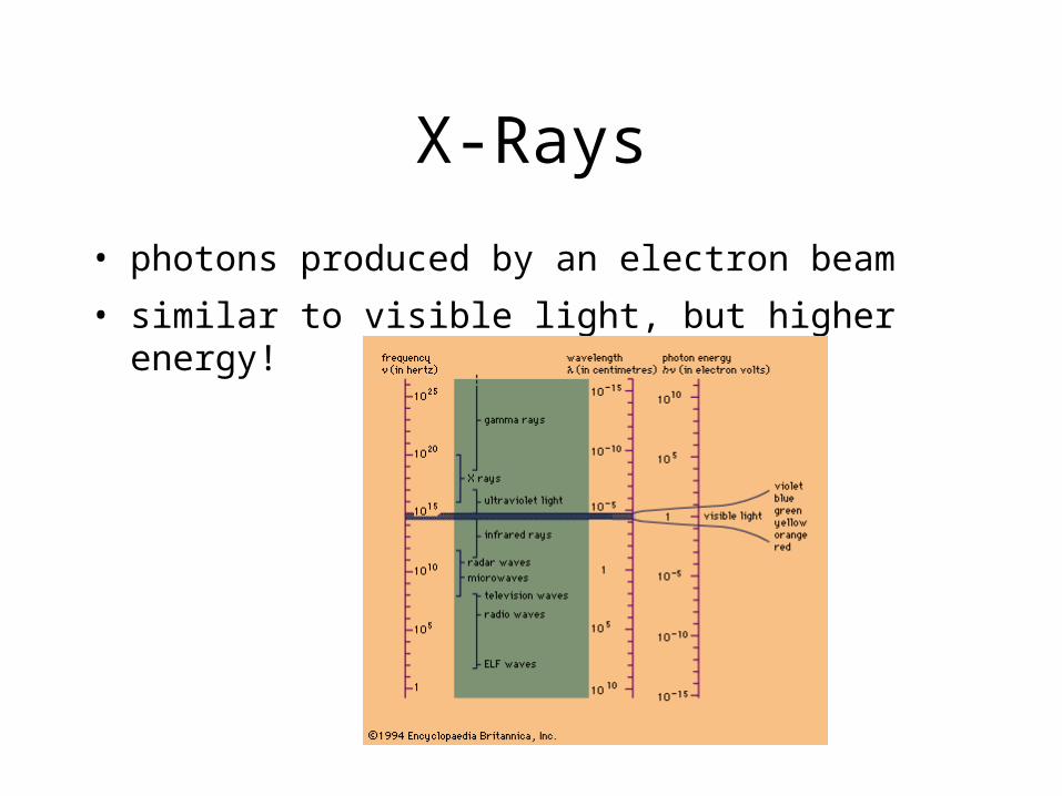
X-Rays

• photons produced by an electron beam

• similar to visible light, but higher energy!

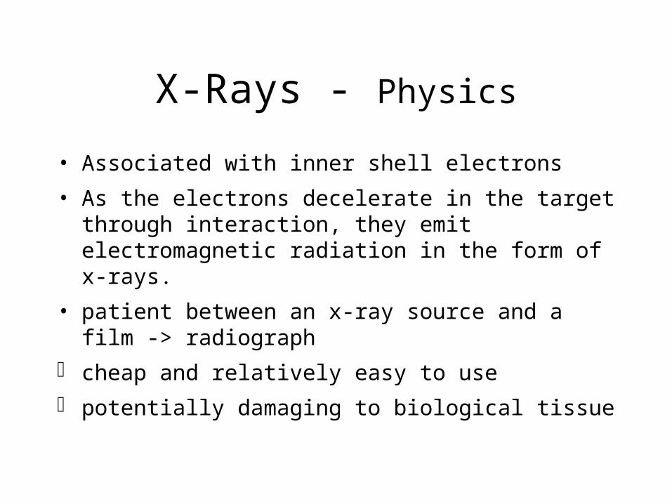
X-Rays - Physics

• Associated with inner shell electrons

• As the electrons decelerate in the target through interaction, they emit electromagnetic radiation in the form of x-rays.

• patient between an x-ray source and a film -> radiograph

cheap and relatively easy to use potentially damaging to biological tissue

X-Rays - Visibility

• bones contain heavy atoms -> with many electrons, which act as an absorber of x-rays

commonly used to image gross bone structure and lungs

excellent for detecting foreign metal objects main disadvantage -> lack of anatomical

structure all other tissue has very similar absorption

coefficient for x-rays

X-Rays - Images

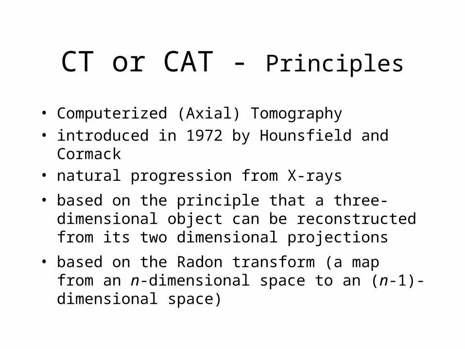
CT or CAT - Principles

• Computerized (Axial) Tomography• introduced in 1972 by Hounsfield and Cormack• natural progression from X-rays

• based on the principle that a three-dimensional object can be reconstructed from its two dimensional projections

• based on the Radon transform (a map from an n-dimensional space to an (n-1)-dimensional space)

CT or CAT - Methods

• measures the attenuation of X-rays from many different angles

• a computer reconstructs the organ under study in a series of cross sections or planes

• combine X-ray pictures from various angles to reconstruct 3D structures

CT - Reconstruction: FBP

• Filtered Back Projection

• common method

• uses Radon transform and Fourier Slice Theorem

f(x,y)

y

x s

g(s)

G()

u

F(u,v)

Spatial Domain Frequency Domain

CT - Reconstruction: ART

• Algebraic Reconstruction Technique

• iterative technique

• attributed to Gordon

Reconstructed

model

Actual Data

Slices

ProjectionBack-

Projection

Initial Guess

CT - FBP vs. ART

• Computationally cheap

• Clinically usually 500 projections per slice

• problematic for noisy projections

• Still slow• better quality for

fewer projections• better quality for

non-uniform project.• “guided” reconstruct.

(initial guess!)

FBP ART

CT - 2D vs. 3D• Linear advancement (slice by

slice)– typical method

– tumor might fall between ‘cracks’

– takes long time

• helical movement– 5-8 times faster

– A whole set of trade-offs

CT or CAT - Advantages

significantly more data is collected superior to single X-ray scans far easier to separate soft tissues other than

bone from one another (e.g. liver, kidney) data exist in digital form -> can be analyzed

quantitatively adds enormously to the diagnostic information used in many large hospitals and medical

centers throughout the world

CT or CAT - Disadvantages

significantly more data is collected soft tissue X-ray absorption still relatively

similar still a health risk MRI is used for a detailed imaging of anatomy

MRI

• Nuclear Magnetic Resonance (NMR) (or Magnetic Resonance Imaging - MRI)

• most detailed anatomical information

• high-energy radiation is not used, i.e. “save”

• based on the principle of nuclear resonance

• (medicine) uses resonance properties of protons

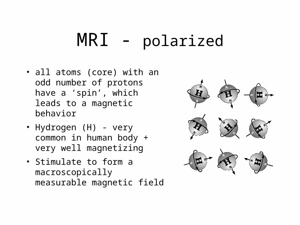
MRI - polarized

• all atoms (core) with an odd number of protons have a ‘spin’, which leads to a magnetic behavior

• Hydrogen (H) - very common in human body + very well magnetizing

• Stimulate to form a macroscopically measurable magnetic field

MRI - Signal to Noise Ratio

• proton density pictures - measures HMRI is good for tissues, but not for bone

• signal recorded in Frequency domain!!

• Noise - the more protons per volume unit, the more accurate the measurements - better SNR through decreased resolution

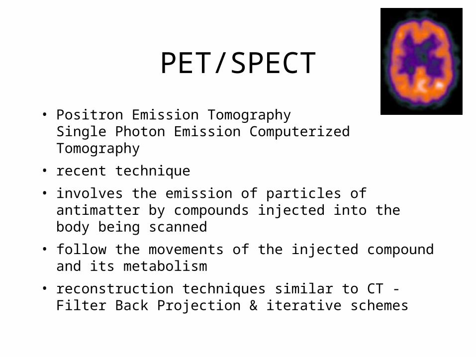
PET/SPECT

• Positron Emission TomographySingle Photon Emission Computerized Tomography

• recent technique

• involves the emission of particles of antimatter by compounds injected into the body being scanned

• follow the movements of the injected compound and its metabolism

• reconstruction techniques similar to CT - Filter Back Projection & iterative schemes

Ultrasound

• the use of high-frequency sound (ultrasonic) waves to produce images of structures within the human body

• above the range of sound audible to humans (typically above 1MHz)

• piezoelectric crystal creates sound waves

• aimed at a specific area of the body

• change in tissue density reflects waves

• echoes are recorded

Ultrasound (2)

• Delay of reflected signal and amplitude determines the position of the tissue

• still images or a moving picture of the inside of the body

• there are no known examples of tissue damage from conventional ultrasound imaging

• commonly used to examine fetuses in utero in order to ascertain size, position, or abnormalities

• also for heart, liver, kidneys, gallbladder, breast, eye, and major blood vessels

Ultrasound (3)

• by far least expensive

• very safe

• very noisy

• 1D, 2D, 3D scanners

• irregular sampling - reconstruction problems

Computational Methods (CM)

• Computational Field Simulations• Computational Fluid Dynamics -

Flow simulations• Computational Chemistry -

Electron-electron interactions, Molecular surfaces

• Computational Mechanics - Fracture

• Computational Manufacturing - Die-casting

CM - Approach

• (Continuous) physical model– Partial/Ordinary Differential Equation (ODE/PDE)– e.g. Navier-Stokes equation for fluid flow– e.g. Hosted Equations:– e.g. Schrödinger Equation - for waves/quantum

• Continuous solution doesn’t exist (for most part)

• Numerical Approximation/Solution1. Discretize solution space - Grid generation explicit2. Replace continuous operators with discrete ones3. Solve for physical quantities

bxaBbfAafxgf xx ,)(,)(:)(

CM - Methods

• Grid Generation– non-elliptical methods:

algebraic, conformal, hyperbolic, parabolic, biharmonic

– elliptical methods (based on elliptical PDE’s)

• Numerical Methods– Newton– Runge-Kutta– Finite Element– Finite Differences

• Time Varying

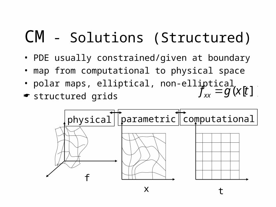
CM - Solutions (Structured)• PDE usually constrained/given at boundary• map from computational to physical space• polar maps, elliptical, non-elliptical structured grids

computationalparametricphysical

fx t

])[( txgf xx

CM - Solutions (Unstructured)

• usually scattered data set• Delaunay Triangulation• Element Size Optimization

– start with initial tetrahedral grid– interactively insert grid points– insertion guided by curvature and distance to surface

• Advancing Front Method– start with boundary– advance boundary towards inside until “filled”

CM - Grid Types (2)

• Multiblock structured grids– multiple structured grids– connected not necessarily structured

• hybrid grids– structured + unstructured

• chimera grids– multiple structured grids– partially overlapping

• hierarchical grids– generated by quad-tree and octree like subdivision

schemes (AKA embedded or semi-structured grids)

CM - Grid Examples

CM - Structured vs. Unstructured

• consider discretization points assamples, points, cells, or voxels

• Structured – Addressing - Cell [i,j,k] provides location of neighbors– Boundaries of volume - Easy to determine

• Unstructured– No addressing mechanism - adjacency list required– Cannot determine the boundaries easily– Cells never of same size– Cells are hexahedrons, tetrahedrons, curved patches

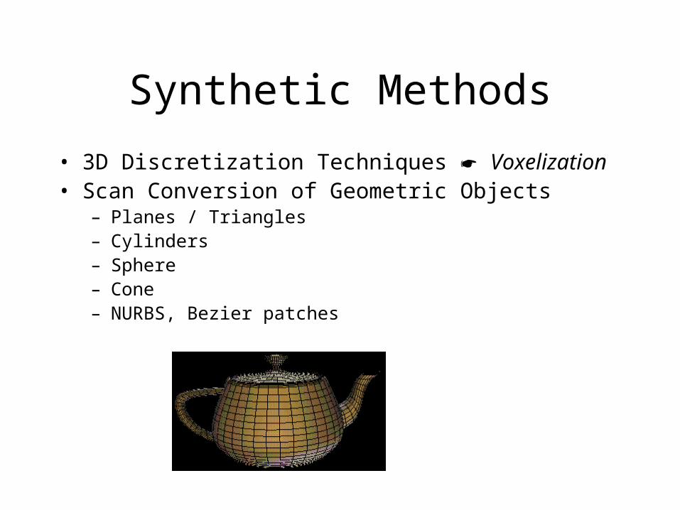
Synthetic Methods

• 3D Discretization Techniques Voxelization• Scan Conversion of Geometric Objects

– Planes / Triangles – Cylinders– Sphere– Cone– NURBS, Bezier patches

Synthetic Methods

• Solid Textures• Hyper Texture - 3D

Textures – Fur– Marble– Hair– Turbulent flow

• 3D Regular grid has texture values

Grid Types

uniform rectilinearregular curvilinear

Structured Grids:

regular irregular hybrid curved

Unstructured Grids:

Data Representation

• Regular – Contour Stacks– Raster– RLE

raster Point list RLE

Data Representation (2)

• Polygon mesh, Curvilinear, Unstructured– Vertex list– Adjacency list of cells (not for curvilinear)– No convenient structure

• Compressed Grids - RLE, JPEG, Wavelets• Multi-resolution Grids

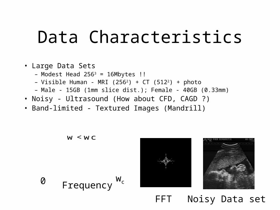
Data Characteristics

• Large Data Sets– Modest Head 2563 = 16Mbytes !!– Visible Human - MRI (2562) + CT (5122) + photo– Male - 15GB (1mm slice dist.); Female - 40GB (0.33mm)

• Noisy - Ultrasound (How about CFD, CAGD ?)• Band-limited - Textured Images (Mandrill)

w < wc

FFT

Frequency0 wc

Noisy Data set

Data Characteristics

• Limited Dynamic Range - values between min, max populated with unequal probability

• Non-Uniform Spatial Occupancy -– Quadtree/Octree– Rectangular spatial subdivision

Data Objects

Data Object: dataset (representation of information)

• Structures: how the information is organized- Topology- Geometry

• Attributes: store the information we want to visualize. e.g. function values

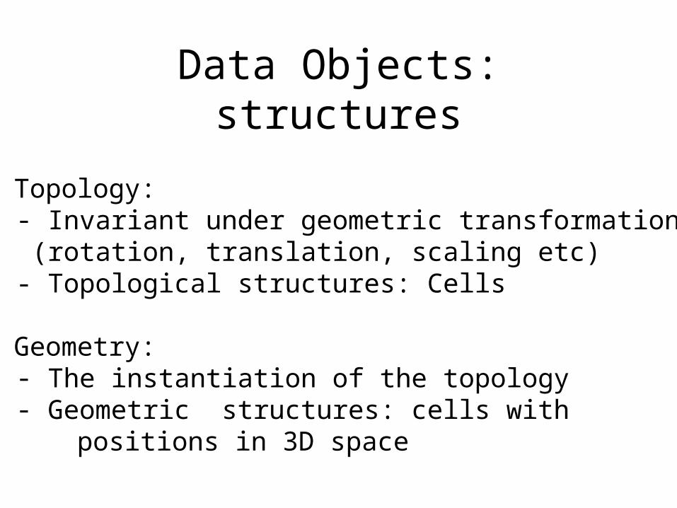
Data Objects: structures

• Topology: - Invariant under geometric transformation (rotation, translation, scaling etc)- Topological structures: Cells

• Geometry: - The instantiation of the topology- Geometric structures: cells with

positions in 3D space

Cell Types for Unstructured Grid

(a) vertex (b) Polyvertex (c) line (d) polyline (e) triangle

(e) Quadrilateral (e) Polygon (f) Tetrahedron(f) Hexahedron

And more (I am too tired drawing now …)

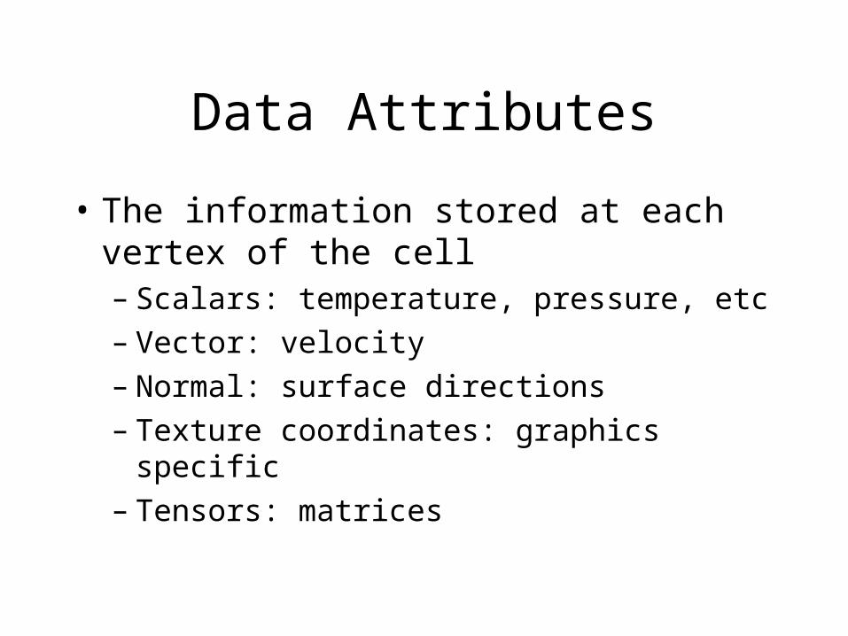
Data Attributes

• The information stored at each vertex of the cell– Scalars: temperature, pressure, etc– Vector: velocity– Normal: surface directions– Texture coordinates: graphics specific– Tensors: matrices

Where are we now ...

Data Object: dataset (representation of information)

• Structures: how the information is organized- Topology- Geometry

• Attributes: store the information we want to visualize. e.g. function values

Remember:

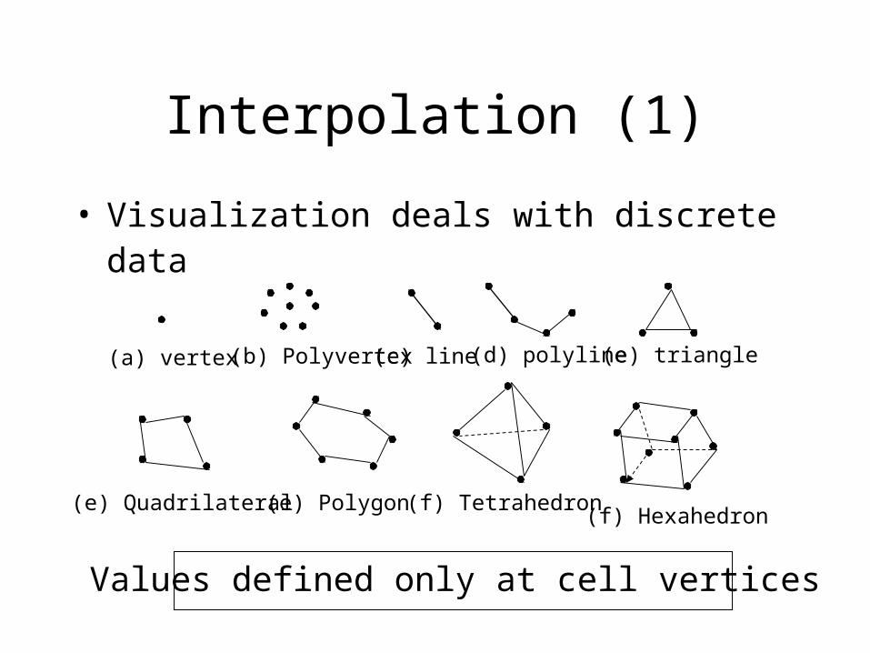
Interpolation (1)

• Visualization deals with discrete data

(a) vertex (b) Polyvertex(c) line (d) polyline (e) triangle

(e) Quadrilateral (e) Polygon (f) Tetrahedron(f) Hexahedron

Values defined only at cell vertices

Color Mapping

R G B

Values at vertices Color lookup Result table

v1v2v3...

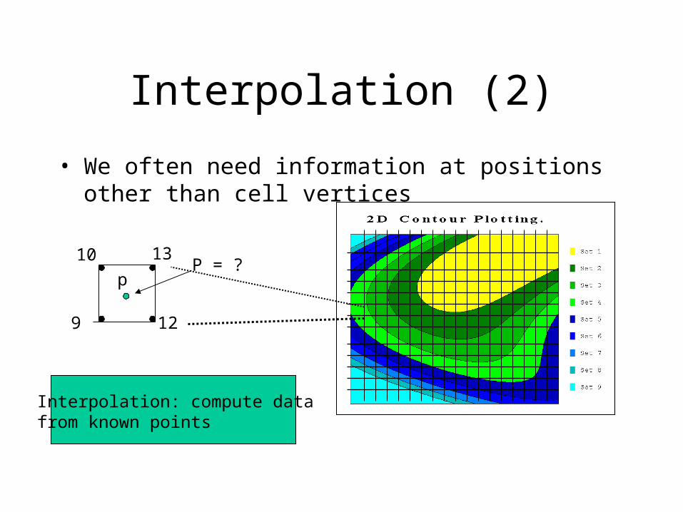
Interpolation (2)

• We often need information at positions other than cell vertices

Interpolation: compute datafrom known points

pP = ?

10 13

9 12

Interpolation (3)

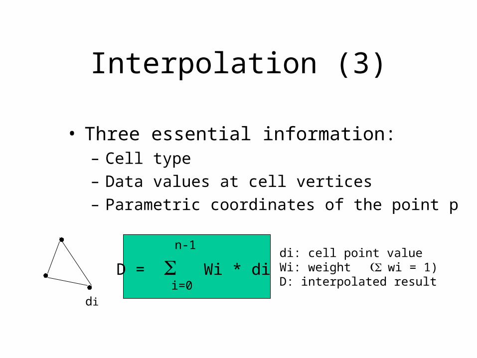
• Three essential information:– Cell type

– Data values at cell vertices

– Parametric coordinates of the point p

D = Wi * di i=0

n-1

di

di: cell point valueWi: weight wi = 1)D: interpolated result

Interpolation (4)

Parametric Coordinates: Used to specify the location of a point within a cell

D = Wi * di i=0

n-1W0 = (1-r)W1 = r

(a) line

r = 0

r = 1

0 <= r <=1d0

d1

r

Interpolation (5)

(b) Triangle

s

rp0 p1

p2

r=0

s=0

r+s = 1 (why?)

W0 = 1-r-sW1 = rW2 = s

Why?

Interpolation (6)

(C) Pixel

p0 p1

p2 p3

r

s

(s,t)

s=0

r=0 r =1

s=1

W0 = (1-r)(1-s)W1 = r(1-s)W2 = (1-r)sW3 = rs

Why?

This is also called bi-linear interpolation

Interpolation (7)

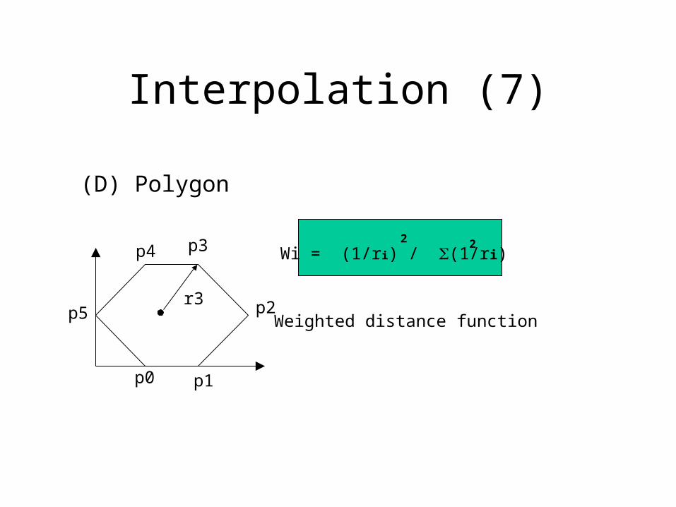
(D) Polygon

p0 p1

p2

p3p4

p5

Wi = (1/ri) / (1/ri)2 2

r3Weighted distance function

Interpolation (8)

(D) Tetrahedron

r

s

t

W0 = 1-r-s-tW1 = rW2 = sW3 = t

p1

p0

p2p3

Interpolation (9)

(D) Cube (voxel)

r

t

s

W0 = (1-r)(1-s)(1-r)W1 = r(1-s)(1-t)W2 = (1-r)s(1-t)W3 = rs(1-r)W4 = (1-r)(1-s)tW5 = r(1-s)tW6 = (1-r)stW7 = rstp0 p1

p2 p3

p4 p5

p6 p7

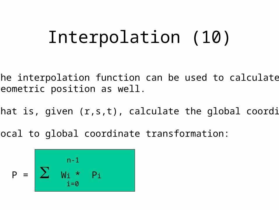
Interpolation (10)

The interpolation function can be used to calculate the geometric position as well.

That is, given (r,s,t), calculate the global coordinates

Local to global coordinate transformation:

P = Wi * Pii=0

n-1

Interpolation (11)

How to get (r,s,t) ?

•Line, Pixel, Cube are all trivial

•Triangle, Tetrahedron can be solved analytically

•Qudrilateral or Hexahedra need numerical method

P = Wi * Pii=0

n-1Known: P, PiUnkown: Wi (i.e. r,s,t)

Contours

3 7

10 4

C = 6

Interpolation

• Given:

• Needed:

2D 1D• Given:

• Needed:

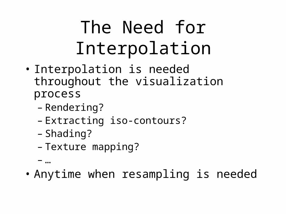
The Need for Interpolation

• Interpolation is needed throughout the visualization process– Rendering?– Extracting iso-contours?– Shading?– Texture mapping?– …

• Anytime when resampling is needed

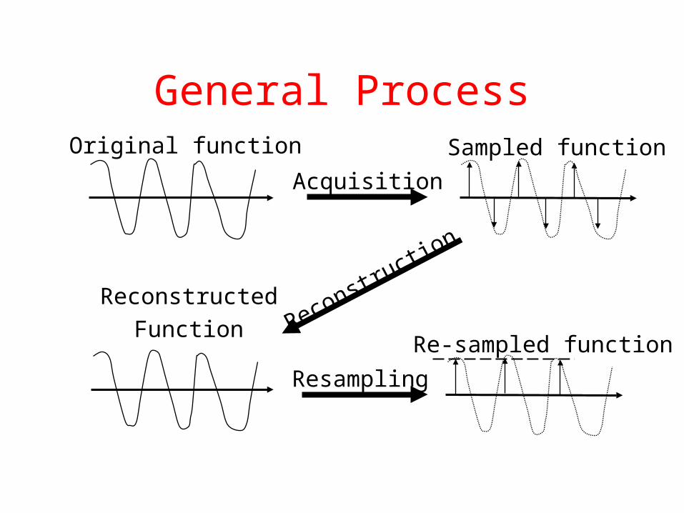
General ProcessOriginal function Sampled function

ReconstructedFunction

Acquisition

Reconstructio

n

Re-sampled function

Resampling

How? - ConvolutionSpatial Domain:

Mathematically:f(x)*h(x) =

dttxgtf

Frequency Domain:

HF

Evaluated at discrete points (sum)

• Multiplication:• Convolution:

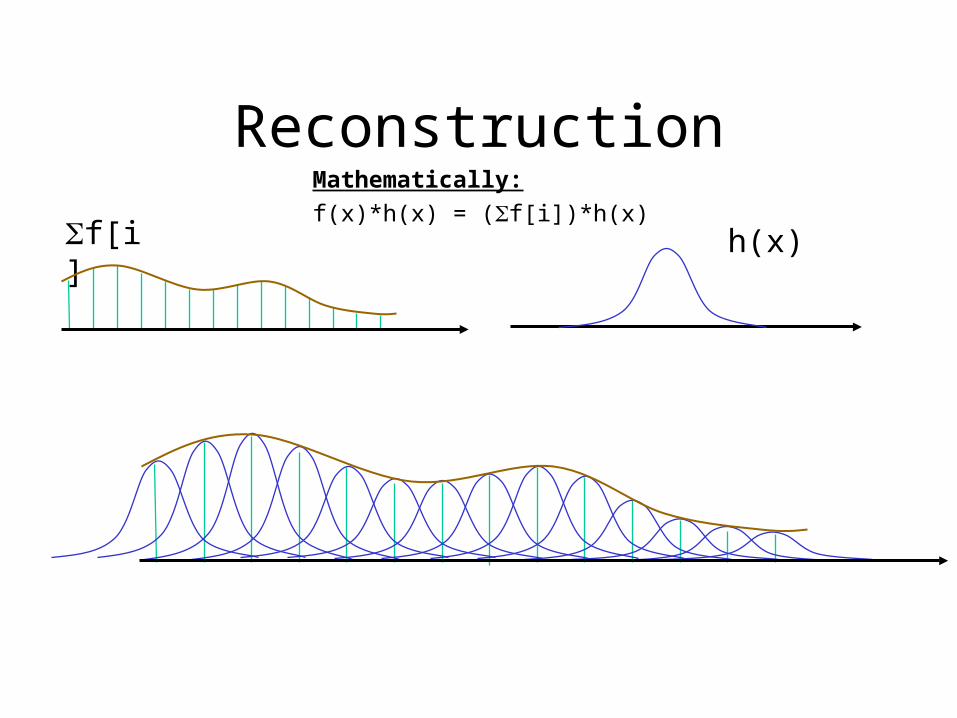
ReconstructionMathematically:f(x)*h(x) = (f[i])*h(x)f[i] h(x)

General Process - Frequency Domain

Acquisition

Reconstructio

n

Resampling

Original function Sampled function

ReconstructedFunction

Re-sampled function

Pre-Filtering

Pre-Filtering

Acquisition

Reconstruction

Original function Band-limited function

SampledFunction

Reconstructed function

Ideal Reconstruction with Sinc function

Spatial Domain:• convolution is exact

Frequency Domain:• cut off freq. replica

0 xfxfr x

xx

sin

Sinc

-0.4

-0.2

0

0.2

0.4

0.6

0.8

1

-25 -20 -15 -10 -5 0 5 10 15 20 250.65

0.7

0.75

0.8

0.85

0.9

0.95

0 0.05 0.1 0.15 0.2 0.25 0.3 0.35 0.4 0.45 0.5

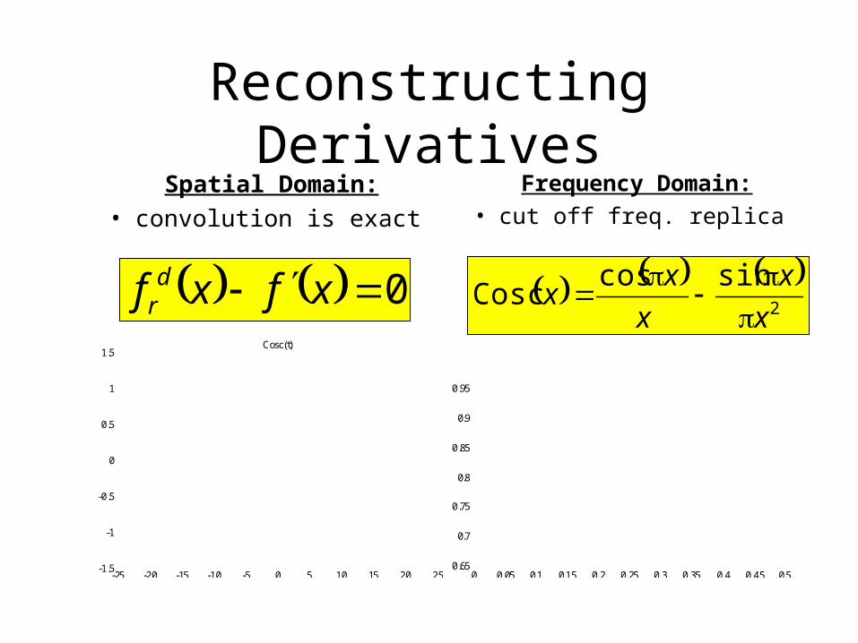
Reconstructing DerivativesSpatial Domain:

• convolution is exactFrequency Domain:• cut off freq. replica

0 xfxf dr

2

sincosCosc

x

x

x

xx

-1.5

-1

-0.5

0

0.5

1

1.5

-25 -20 -15 -10 -5 0 5 10 15 20 25

Cosc(t)

0.65

0.7

0.75

0.8

0.85

0.9

0.95

0 0.05 0.1 0.15 0.2 0.25 0.3 0.35 0.4 0.45 0.5

Possible Errors• Post-aliasing

– reconstruction filter passes frequencies beyond the Nyquist frequency (of duplicated frequency spectrum) => frequency components of the original signal appear in the reconstructed signal at different frequencies

• Smoothing– frequencies below the Nyquist frequency are attenuated

• Ringing (overshoot)– occurs when trying to sample/reconstruct discontinuity

• Anisotropy– caused by not spherically symmetric filters

How Good? = ErrorSpatial Domain:

• local error• asymptotic error• numerical error

Frequency Domain:• global error• visual appearance• blurring• aliasing• smoothing

ApproximationTheory/Analysis

Signal Processing

Sources of Aliasing• Non-bandlimited signal

• Low sampling rate (below Nyquist)

• Non perfect reconstruction

Reconstruction Kernels

stop bandpass band

Smoothing error

Postaliasing error

Ideal filter

filter

The spatial extent of reconstruction kernels, or interpolation basis functions, depend on the cut-off frequency as well.

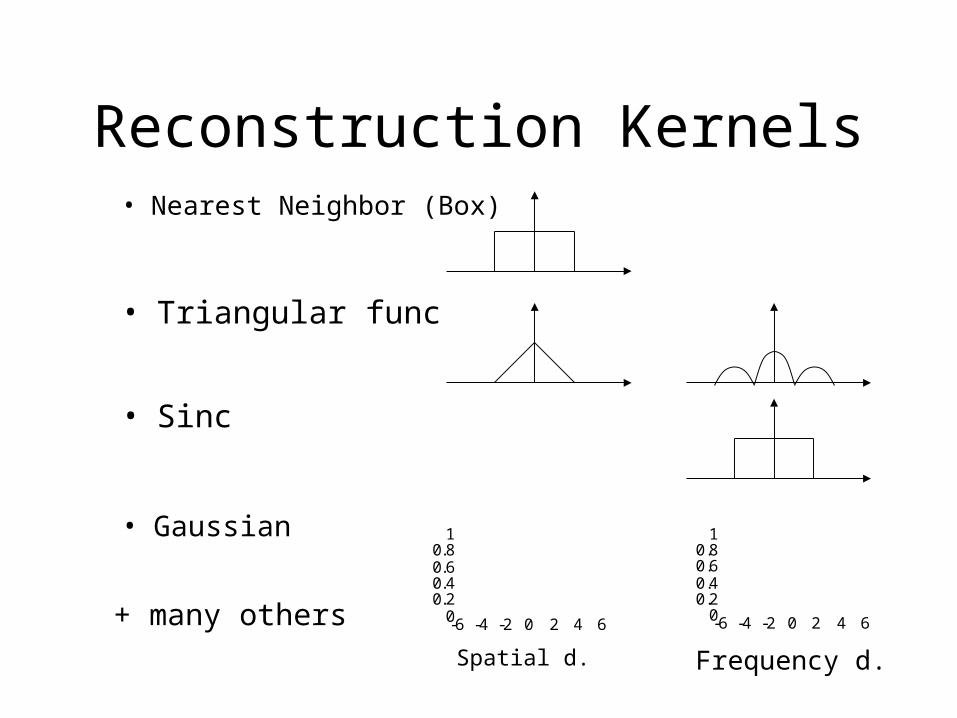
Reconstruction Kernels• Nearest Neighbor (Box)

00.20.40.60.81

-6 -4 -2 0 2 4 60

0.20.40.60.81

-6 -4 -2 0 2 4 6

• Triangular func

• Sinc

• Gaussian

+ many others

Spatial d. Frequency d.

Higher Dimensions• An-isotropic Filters• (radially symmetric)

• separable filters

yhxhyxh , 22, yxhyxh

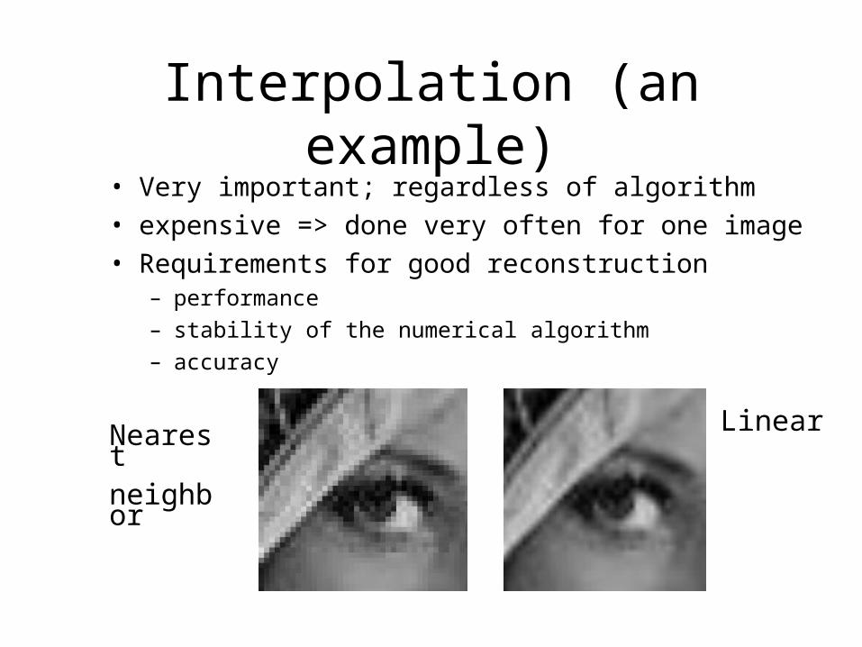
Interpolation (an example)• Very important; regardless of algorithm• expensive => done very often for one image• Requirements for good reconstruction

– performance– stability of the numerical algorithm– accuracy

Nearestneighbor

Linear

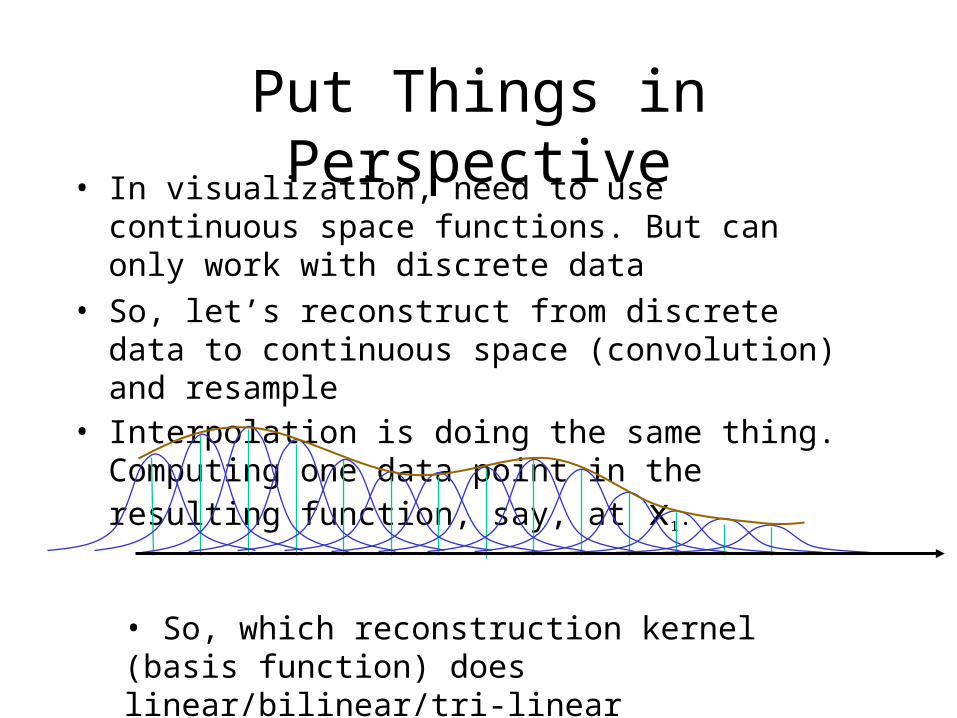
Put Things in Perspective• In visualization, need to use continuous space functions.

But can only work with discrete data

• So, let’s reconstruct from discrete data to continuous space (convolution) and resample

• Interpolation is doing the same thing. Computing one data point in the resulting function, say, at x1.

• So, which reconstruction kernel (basis function) does linear/bilinear/tri-linear interpolations use?