Institut f¨ ur Signalverarbeitung und Prozessrechentechnik der Universit¨ at zu L¨ ubeck Direktor: Prof. Dr.-Ing. Alfred Mertins Data Acquisition and Processing System for Multisite Neural Recordings Inauguraldissertation zur Erlangung der Doktorw¨ urde (Dr.-Ing.) der Universit¨ at zu L¨ ubeck – Technisch-Naturwissenschaftliche Fakult¨at – vorgelegt von Diplom-Informatiker Andre Folkers aus Westerstede L¨ ubeck, Oktober 2008

Welcome message from author
This document is posted to help you gain knowledge. Please leave a comment to let me know what you think about it! Share it to your friends and learn new things together.
Transcript
Institut fur Signalverarbeitung und Prozessrechentechnikder Universitat zu Lubeck
Direktor: Prof. Dr.-Ing. Alfred Mertins
Data Acquisition and Processing System forMultisite Neural Recordings
Inauguraldissertationzur Erlangung der Doktorwurde (Dr.-Ing.)
der Universitat zu Lubeck– Technisch-Naturwissenschaftliche Fakultat –
vorgelegt vonDiplom-Informatiker Andre Folkers
aus Westerstede
Lubeck, Oktober 2008

1. Berichterstatter: Professor Dr. Ulrich G. Hofmann2. Berichterstatter: Professor Dr. Dr. Siegfried J. Poppl

Vorwort
”Lubeck ist ’ne schone Stadt, weil sie sieben Turme hat!”, so schallt es jetzt oft
von den hinteren Sitzen des Autos, wenn ich mit meiner Familie unterwegs bin.Als Stadt zum Studieren hatte ich damals Lubeck vor allem wegen des dort ange-botenen Nebenfachs Medizinische Informatik gewahlt. Wie sich herausstellte, wares eine gute Wahl. Aus der Verbindung von Informatik und Medizin ergaben sichschon wahrend des Studiums viele interessante Aufgaben fur Seminare und Prakti-ka. So war ich froh, dass ich nach Abschluss meines Informatikstudiums am Institutfur Signalverarbeitung und Prozessrechentechnik (ISIP) die Moglichkeit bekam, alswissenschaflicher Mitarbeiter genau auf dieser Schnittstelle zu arbeiten.
Fur die Unterstutzung, die ich von meinen Kollegen, Freunden und von meinerFamilie erhalten habe, mochte ich mich bedanken. Besonderer Dank gebuhrt dabeimeinem Doktorvater Herrn Privatdozent Ulrich G. Hofmann, der meine Arbeit her-vorragend betreut hat und dessen Ideen und Engagement es mir ermoglicht haben,diese Arbeit zu erstellen. Fur die freundschaftliche Zusammenarbeit danke ich auchmeinen Kollegen Alexandru Condurache, Kerstin Menne, Ingo Stuke und DanielToth.
Florian Mosch und Thomas Malina danke ich fur ihren Beitrag, den sie im Rah-men ihrer Diplomarbeiten bei der Entwicklung des Datenaufnahmesystems geleistethaben. Fur die Durchsicht der Dissertation bedanke ich mich bei Olaf Christ undbei Dr. Peter Vorlander.
Bei Herrn Professor Til Aach mochte ich mich fur die freundliche Aufnahme amISIP und fur sein fachliches Interesse an meiner Arbeit bedanken und bei HerrnProfessor Alfred Mertins fur seine Unterstutzung in der Endphase der Arbeit. Furdie Ubernahme des Koreferats danke ich Herrn Professor Siegfried J. Poppl und furden Vorsitz der Prufungskommission Herrn Professor Thomas Martinetz.
Bei den Projektpartnern aus dem VSAMUEL Konsortium mochte ich mich furdie gute und produktive Zusammenarbeit bedanken. Fur die Einblicke in ihre ex-perimentelle Arbeit und die Evaluierung des Systems danke ich Marco de Curtisund Gerardo Biella vom Nationalen Institut fur Neurophysiologie in Mailand, KenYoshida und Winnie Jensen der Universitat Aalborg, Erik de Schutter, Patriq Fa-gerstedt und Antonia Volny-Luraghi von Universitat Antwerpen. Thomas Recordingdanke ich dafur, dass ich die Entwicklung des Datenaufnahmesystem bei ihnen nocheinige Monate fortfuhren konnte. Eine eine weitere Moglichkeit, dass Datenaufnah-mesystem im experimentellen Umfeld zu testen, verdanke ich Winrich Freiwald undHeiko Stemman von der Universitat Bremen.
Mein besonderer Dank gilt meiner Familie, die mich in großartiger Weise un-terstutzt hat. Ohne ihre Unterstutzung ware diese Arbeit wohl kaum jemals ferti-
iii

VORWORT iv
gestellt worden. Meinen Eltern Enno und Christiane Folkers danke ich dafur, dasssie mir mein Studium ermoglicht haben, das die Grundlage fur diese Arbeit bildet.Bei meinen Schwiegereltern Arthur und Ursula Springfeld bedanke ich mich dafur,dass sie mir durch ihre Hilfe so manche Stunde Zeit verschafft haben. Meinen Kin-dern Antonia, Karolin, Frederik und Teresa danke fur die Frohlichkeit mit der siemir Motivation gegeben haben. Den großten Dank mochte ich meiner Frau Verenaaussprechen, die mich immer wieder dazu gebracht hat weiterzumachen.
Fur meine Familie
Verl, im Oktober 2008

Contents
Vorwort iii
Zusammenfassung viii
Summary xi
1 Introduction 1
2 Neural activity 42.1 Nervous system . . . . . . . . . . . . . . . . . . . . . . . . . . . . . . 42.2 Neural cell . . . . . . . . . . . . . . . . . . . . . . . . . . . . . . . . . 5
2.2.1 Morphological classification . . . . . . . . . . . . . . . . . . . 72.2.2 Functional classification . . . . . . . . . . . . . . . . . . . . . 7
2.3 Glial cells . . . . . . . . . . . . . . . . . . . . . . . . . . . . . . . . . 92.4 Layered structure of the brain . . . . . . . . . . . . . . . . . . . . . . 92.5 Action potentials . . . . . . . . . . . . . . . . . . . . . . . . . . . . . 9
2.5.1 Membrane potential . . . . . . . . . . . . . . . . . . . . . . . 102.5.2 Action potential generation . . . . . . . . . . . . . . . . . . . 12
2.6 Field potentials . . . . . . . . . . . . . . . . . . . . . . . . . . . . . . 132.7 Tuning curves and information coding . . . . . . . . . . . . . . . . . 14
3 Neural signal acquisition 173.1 Sensing bioelectrical signals . . . . . . . . . . . . . . . . . . . . . . . 193.2 Extracellular potentials . . . . . . . . . . . . . . . . . . . . . . . . . . 203.3 Probes for intracavitary or intratissue recordings . . . . . . . . . . . . 203.4 Silicon-based mulitchannel microelectrodes . . . . . . . . . . . . . . . 223.5 Manufacturing VSAMUEL probes . . . . . . . . . . . . . . . . . . . . 23
4 Signal processing 274.1 Digital filter . . . . . . . . . . . . . . . . . . . . . . . . . . . . . . . . 27
4.1.1 FIR and IIR filter . . . . . . . . . . . . . . . . . . . . . . . . . 294.2 Wavelet Transformation . . . . . . . . . . . . . . . . . . . . . . . . . 30
4.2.1 Wavelet filter bank . . . . . . . . . . . . . . . . . . . . . . . . 334.2.2 Translation invariance . . . . . . . . . . . . . . . . . . . . . . 35
4.3 Fast lifting wavelet transform . . . . . . . . . . . . . . . . . . . . . . 364.3.1 Example . . . . . . . . . . . . . . . . . . . . . . . . . . . . . . 414.3.2 Mapping onto integer values . . . . . . . . . . . . . . . . . . . 43
v
CONTENTS vi
4.3.3 Implementing lifting steps on a C6701 . . . . . . . . . . . . . 45
5 Applying Wavelet Transform to Neural Signals 515.1 Low pass, band pass, and high pass wavelet filter . . . . . . . . . . . 515.2 Compression and Denoising . . . . . . . . . . . . . . . . . . . . . . . 515.3 Spike detection . . . . . . . . . . . . . . . . . . . . . . . . . . . . . . 545.4 Spike sorting . . . . . . . . . . . . . . . . . . . . . . . . . . . . . . . 55
5.4.1 Spike features . . . . . . . . . . . . . . . . . . . . . . . . . . . 575.4.2 Principal component analysis . . . . . . . . . . . . . . . . . . 585.4.3 Online wavelet based spike sorting . . . . . . . . . . . . . . . . 59
6 Data Acquisition System 646.1 Hardware . . . . . . . . . . . . . . . . . . . . . . . . . . . . . . . . . 64
6.1.1 Probes . . . . . . . . . . . . . . . . . . . . . . . . . . . . . . . 646.1.2 Amplifier . . . . . . . . . . . . . . . . . . . . . . . . . . . . . 656.1.3 AD conversion . . . . . . . . . . . . . . . . . . . . . . . . . . . 686.1.4 Digital signal processor board M67 . . . . . . . . . . . . . . . 716.1.5 Synchronization . . . . . . . . . . . . . . . . . . . . . . . . . . 736.1.6 Host PC . . . . . . . . . . . . . . . . . . . . . . . . . . . . . . 746.1.7 Thermal issues . . . . . . . . . . . . . . . . . . . . . . . . . . 75
6.2 Software . . . . . . . . . . . . . . . . . . . . . . . . . . . . . . . . . . 776.2.1 DSP application . . . . . . . . . . . . . . . . . . . . . . . . . . 776.2.2 Host application . . . . . . . . . . . . . . . . . . . . . . . . . 82
7 Biological validation 1037.1 Recording from the guinea pig brain . . . . . . . . . . . . . . . . . . 103
7.1.1 Isolation of the guinea pig brain . . . . . . . . . . . . . . . . . 1047.1.2 Recordings in the medial entorhinal cortex . . . . . . . . . . . 104
7.2 Recordings from rat cerebellum . . . . . . . . . . . . . . . . . . . . . 110
8 Discussion 112
A Microstructure techniques 115A.1 Metal evaporation . . . . . . . . . . . . . . . . . . . . . . . . . . . . . 115A.2 Lift-off process . . . . . . . . . . . . . . . . . . . . . . . . . . . . . . 115A.3 PECVD . . . . . . . . . . . . . . . . . . . . . . . . . . . . . . . . . . 116A.4 Deep RIE . . . . . . . . . . . . . . . . . . . . . . . . . . . . . . . . . 116
B M67 and Ad16 extensions and modifications 118B.1 SyncLink and ClockLink . . . . . . . . . . . . . . . . . . . . . . . . . 118B.2 Synchronizing the AD16 boards . . . . . . . . . . . . . . . . . . . . . 120B.3 Trigger Input . . . . . . . . . . . . . . . . . . . . . . . . . . . . . . . 120
C Realtime operating system 122C.1 Overview . . . . . . . . . . . . . . . . . . . . . . . . . . . . . . . . . . 122C.2 Texas Instruments DSP/BIOS . . . . . . . . . . . . . . . . . . . . . . 123
C.2.1 Threads . . . . . . . . . . . . . . . . . . . . . . . . . . . . . . 123

CONTENTS vii
C.2.2 Interthread communication and synchronization . . . . . . . . 124C.2.3 Timer . . . . . . . . . . . . . . . . . . . . . . . . . . . . . . . 125C.2.4 Profiling . . . . . . . . . . . . . . . . . . . . . . . . . . . . . . 125

Zusammenfassung
Die hier vorgelegte Arbeit ist im Rahmen des EU-geforderten Projekts VSAMUEL(Development of a Versatile System for Advanced Neuronal Recordings with Multi-site Microelectrodes) entstanden. Ziel des Projektes war es, ein leicht verwendbaresSystem zur Aufzeichnung von verschiedenen neurophysiologischen Signalen in le-bendem Nervengewebe zu entwickeln. Die schwedische Firma Acreo hat dabei mitMikrostrukturtechniken gefertigte Sonden auf Siliziumbasis entwickelt und herge-stellt, die bis zu 64 Aufzeichnungspunkte besitzen. Von der deutschen Firma ThomasRecording aus Gießen wurden passende Vor- und Hauptverstarker entworfen und ge-baut. Die Aufgabe des Instituts fur Signalverarbeitung und Prozessrechentechnik derUniversitat zu Lubeck war die Entwicklung eines Datenaufnahmesystems, welchesin dieser Arbeit im Besonderen dargestellt wird. Das komplette System wurde inZusammenarbeit mit den Projektpartnern aus verschiedenen Bereichen der neuro-physiologischen Grundlagenforschung praktisch evaluiert.
Die Informationsverarbeitung des zentralen und des peripheren Nervensystemsbasiert im Wesentlichen auf der Kommunikation von Nervenzellen, die sich sowohlanatomisch als auch durch ihre Funktion unterscheiden. Trotzdem sind sie sich in ih-rem grundsatzlichen Aufbau ahnlich. Eine typische Nervenzelle hat einen Zellkorperaus dem ein oft stark verzweigter Dendritenbaum und ein weniger verzweigtes Axonhervorgeht. Das Axon hat an seinen Enden jeweils eine Synapse uber die eine chemi-sche, auf Neurotransmittern basierende Verbindung zu anderen Nervenzellen herge-stellt wird. Vereinfacht gesagt sammelt eine Nervenzelle ihre Eingaben am Dendri-tenbaum und gibt ihre Ausgaben uber das Axon weiter. Ausgaben werden in Formvon Aktionspotentialen im Zellkorper am Ansatzpunkt des Axons gebildet, wenn dieZelle durch inhibitorische oder exzitatorische Eingaben an ihrem Dendritenbaum inSumme uber einen bestimmten Schwellwert hinaus depolarisiert worden ist. Somitspiegeln einzelne Aktionspotentiale die Aktivitat von einzelnen Nervenzellen wider.Die Potentiale an den synaptischen Verbindungen und insbesondere die synchro-nen Anderungen durch die Aktivitat einer großen Gruppe von Nervenzellen addiertsich zu sogenannten Feldpotentialen. Bemerkenswert ist dabei, dass Feldpotentialeallem Anschein nach nicht direkt durch synchron erzeugte Aktionspotentiale ent-stehen. Die genauere Untersuchung des Zusammenhangs zwischen Feldpotentialenund Aktionspotentialen und dessen Bedeutung fur die Informationsverarbeitung imNervensystem erfordert die zeitgleiche Messung von beiden Potentialarten in einermoglichst großen Region.
Die im VSAMUEL Projekt entwickelten gabelformigen Siliziumsonden ermog-lichen Messungen von bis zu 64 Aufzeichnungspunkten pro Sonde. Die effektiveNutzung dieser Sonden erfordert neben ensprechenden Vor- und Hauptverstarker-
viii
ZUSAMMENFASSUNG ix
stufen ein leistungsfahiges Datenaufnahmesystem, das simultan von vielen Kanalenmit hoher Auflosung aufzeichnen kann und diese Daten in Echtzeit verarbeitet.
Ziel beim Entwurf der Signalverarbeitungsmethoden war die Entwicklung einesRahmens zur Echtzeitverarbeitung, der verschiedene Verarbeitungs- und Analyse-moglichkeiten bietet. Das Datenaufnahmesystem berechnet dabei mit Hilfe der Wavelet-Transformation eine Zeit-Frequenz-Analyse der aufgenommenen Daten. Basierendauf den resultierenden Wavelet Koeffizienten konnen die aufgenommenen Signalekomprimiert oder entrauscht werden. Weiter ist es moglich Hochpass-, Bandpass-oder Tiefpassfilter zu realisieren. Die echtzeitfahige Implementierung der Wavelet-zerlegung basiert auf dem sogenannten Lifting Schema. Diese Methode zerlegt eineStufe einer Wavelet Filterbank in mehrere sogenannte Lifting Schritte, wobei red-undante Berechnungen, die bei einer naiven Implementierung auftreten, vermiedenwerden, was wiederum die Anzahl der benotigten Instruktionen verringert. In Rah-men der Arbeit ist ein Tool entwickelt worden, welches aus gegebenen Lifting Schrit-ten optimierten Assembler Code fur den C6701 oder einen Pentium III erzeugt.
Bei der Aufzeichnung von Aktionspotentialen ist deren Detektion basierend aufSchwellwerten und Darstellung vorgesehen. Die Klassifikation von aufgezeichnetenAktionspotentialen auf Basis der in Echtzeit berechneten Waveletkoeffzienten warnicht moglich, da durch die Translationsvarianz der verwendeten dyadischen Wa-veletzerlegung mit Unterabtastung die Varianz in den Koeffizienten zu stark war.Einen vielversprechender Ansatz, dieses Problem zu uberwinden, liegt in der Dual-Tree Complex Wavelet Transformation.
Das Datenaufnahmesystem basiert auf der DSP Karte M67 von Innovative In-tegration (Thousand Oaks, Kalifornien, USA), die mit dem C6701 Prozessor vonTexas Instruments bestuckt ist. Die M67 Karte wurde mit zwei A/D Wandler Mo-dulen vom Typ AD16 desselben Herstellers erweitert. Jedes AD16 Modul kann simul-tan 16 Kanale mit einer Abtastrate von 50 kHz und 16 bit Auflosung aufzeichnen.Durch Synchronisation der zwei AD16 Module pro M67 Karte und durch weite-re Synchronisation von bis zu vier M67 Karten wurde ein Datenaufnahmesystemfur 128 Kanale gebaut. Auf jeder Karte wird eine DSP Applikation ausgefuhrt, diedie aufgezeichneten Daten verarbeitet und uber den PCI Bus in den Speicher desHostrechners transferiert. Die Datenaufnahmeapplikation auf dem Hostrechner fugtdie Daten von den einzelnen Karten zu einem Datenstrom zusammen und speichertsie dann in einer Datei. Zu Beginn einer Aufzeichnung wird die verwendete Sonde,die Abtastrate und die Art der Filterung festgelegt. Ferner man kann die Kanalegruppieren und dabei pro Gruppe weitere Aufzeichnungsparameter definieren.
Die Datenaufnahmeapplikation verwaltet eine frei erweiterbare Liste von Sonden,wobei jeweils das Layout der Aufzeichnungspunkte und deren Zuordnung zu denKanalen am Verstarker hinterlegt sind. uber eine aus diesen Daten erzeugte schema-tische Darstellung der Sonde kann man die Verstarkungsfaktoren fur die Aufzeich-nungpunkte verandern und an den programmierbaren Hauptverstarker ubertragen.
Die aufgezeichneten Daten konnen in einem virtuellen Oszilloskop oder in einemBlueplot dargestellt werden. Der Blueplot zeigt die Amplitude der Kanale farblichkodiert an und ermoglicht die gleichzeitige Darstellung besonders vieler Kanale. DieDatenaufnahmeapplikation kann fur einen einzelnen frei wahlbaren Kanal ein Spek-trogramm anzeigen. Weiter ist es moglich fur eine Auswahl an Kanalen, die vom

ZUSAMMENFASSUNG x
Anwender festgelegt werden kann, Wavelet basierte Filter und Entrauschungsalgo-rithmen zu konfigurieren und zu aktivieren.
Das Datenaufnahmesystem wurde zusammen mit Projektpartnern aus der neu-rophysiologischen Forschung im praktischen Einsatz erprobt. Die Forschungsgruppeam Institut fur Theoretische Neurobiologie der Universitat Antwerpen hat dabei mitder 64 Kanal Variante des Datenaufnahmesystems erfolgreich Aktionspotentiale voneinzelnen und auch von mehreren Zellen im Kleinhirn von Ratten aufgezeichnet. Dieam VSAMUEL Projekt beteiligte Forschungsgruppe vom Nationalen Institut furNeurologie in Mailand, Italien, hat mit einem Prototypen des Datenaufnahmesy-stems Feldpotentiale und auch Aktionspotentiale in einer in-vitro Praparation einesMeerschweinchen-Gehirns gemessen.
Das VSAMUEL Projekt konnte also mit der erfolgreichen Entwicklung eineskompletten, integrierten neurophysiologischen Datenaufnahmesystems basierend aufallgemein verfugbaren DSP Karten und neu entwickelten Siliziumsonden abgeschlos-sen werden.

Summary
The work presented in this thesis was part of the EU-funded project VSAMUEL(Development of a Versatile System for Advanced Neuronal Recordings with Multi-site Microelectrodes), which aims to develop easy-to-use instrumentation for multi-channel recordings from functioning and living nervous tissue. It integrates advancedmicro structuring techniques to batch fabricate multi-site microelectrode probes withnovel PC based real-time data acquisition and signal processing.
The main objective of this PhD thesis is to develop a data acquisition systemprototype which allows simultaneous recording from 128 channels at 50 kHz perchannel with 16 bit resolution and the signal processing. The signal processingincludes a wavelet based digital filter, the detection of action potentials and theirclassification. A core component of the data acquisition system is a DSP boardwhich is used for data acquisition and for digital filtering. The host PC softwareprovides different means of visualization and online processing, like e.g. virtualscope, blue plot, and spectrogram. A graphical user interface for data acquisition,data review, and data analysis has been developed with respect to a good design,usability, and speed. The whole system is evaluated together with experimentalpartners for different application area, i.e. peripheral nerves, cerebellum, and cortex.
xi
Chapter 1
Introduction
Ob wir nun aber unsere Bemuhung bloß fur anatomisch erklaren; somußte sie doch, wenn sie fruchtbar, ja wenn sie in unserem Falle auchnur moglich sein sollte, stets in physiologischer Rucksicht unternommenwerden. Man hat also nicht bloß auf das Nebeneinandersein der Teilezu sehen, sondern auf ihren lebendigen, wechselseitigen Einfluß, auf ihreAbhangigkeit und Wirkung.
Johann Wolfgang von Goethe(Entwurfe zu einem osteologischen Typus, 1796)
The nervous system is one of the most complex systems developed by nature.Over centuries scientists have tried to reveal the secrets of our brain [55]. Hip-pocrates (460-379 b.c.) identified the brain as being responsible for our sensationand intelligence. In the 16th century the macroscopic anatomy of the brain wasexamined by Leonardo da Vinci and Andreas Vesalius. In the end of the 18th cen-tury Luigi Galvani found that nerves and muscles can be stimulated by electricity.About 50 years later Jan Purkinje and Theodor Schwann described the microscopicstructure of the brain and the peripheral nerves. Only in the last decades scien-tists had the technical instruments to measure activity of single neurons directly.A.L. Hodgkin and A.F. Huxley were the first, who derived and interpreted actionpotentials from inside neurons.
With this effort many details about the anatomic and physiologic structure havebeen found. However still, the brain is the least understood organ of our body [99].The progress of the neurophysiological research was accompanied by a technicalprogress of measurement instruments. The behaviour of single neurons has beenexamined in-depth [62]. During the last decade the focus of research has moved onto the interaction details between multiple neurons [81] . For future research it isnecessary to have probes which can intercept the activity of multiple single neuronsworking together. Such probes have to be designed with respect to many constraints,e.g. not damaging the tissue, physical stability, and signal quality. Furthermore,in order to truly find insights into the interactions among several neurons, it ismandatory to record their activity at many positions. This will lead to a hugeamount of multichannel data which needs to be acquired and analysed.
1
CHAPTER 1. INTRODUCTION 2
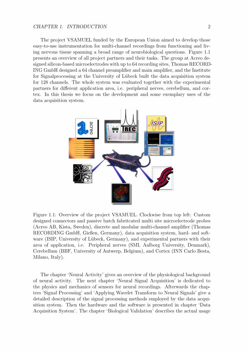
The project VSAMUEL funded by the European Union aimed to develop thoseeasy-to-use instrumentation for multi-channel recordings from functioning and liv-ing nervous tissue spanning a broad range of neurobiological questions. Figure 1.1presents an overview of all project partners and their tasks. The group at Acreo de-signed silicon-based microelectrodes with up to 64 recording sites, Thomas RECORD-ING GmbH designed a 64 channel preamplifier and main amplifier, and the Institutefor Signalprocessing at the University of Lubeck built the data acquisition systemfor 128 channels. The whole system was evaluated together with the experimentalpartners for different application area, i.e. peripheral nerves, cerebellum, and cor-tex. In this thesis we focus on the development and some exemplary uses of thedata acquisition system.
Figure 1.1: Overview of the project VSAMUEL. Clockwise from top left: Customdesigned connectors and passive batch fabritcated multi site microelectrode probes(Acreo AB, Kista, Sweden), discrete and modular multi-channel amplifier (ThomasRECORDING GmbH, Gießen, Germany), data acquisition system, hard- and soft-ware (ISIP, University of Lubeck, Germany), and experimental partners with theirarea of application, i.e. Peripheral nerves (SMI, Aalborg University, Denmark),Cerebellum (BBF, University of Antwerp, Belgium), and Cortex (INN Carlo Besta,Milano, Italy).
The chapter ‘Neural Activity’ gives an overview of the physiological backgroundof neural activity. The next chapter ‘Neural Signal Acquisition’ is dedicated tothe physics and mechanics of sensors for neural recordings. Afterwards the chap-ters ‘Signal Processing’ and ‘Applying Wavelet Transform to Neural Signals’ give adetailed description of the signal processing methods employed by the data acqui-sition system. Then the hardware and the software is presented in chapter ‘DataAcquisition System’. The chapter ‘Biological Validation’ describes the actual usage

CHAPTER 1. INTRODUCTION 3
of the system by the experimental partner of the project. Finally, the discussionreviews the positive and negative results of this work and explains the advantagesand limitations of the proposed system.

Chapter 2
Neural activity
2.1 Nervous system
All kinds of higher animals living on earth have a nervous system. It occurs in a widerange of complexity and, depending on this complexity, it can provide its owner awide range of services. Simple organisms use their nervous system just to accomplishbasic and essential tasks like e.g. finding food or mates for reproduction. With anincreasing complexity of the nervous system the tasks it can perform become morecomplex as well. Humans for instance have a very large nervous system with about1011 (100 billion) neural cells or neurons and additionally 10 to 50 times this numberof glial cells [61]. This complex nervous system is the place where thinking, feeling,consciousness and subconsciousness of humans is located.
The two main types of cells occurring in the nervous systems are neural cellsand glial cells. The neural cells – also called neurons – perform the informationprocessing, while the glial cells are assumed to mainly have support functions. Theysustain the brain structure, transport nutrients from blood to neurons and they forminsulation layers, which speed up information transmissions between neurons [61].
The nervous system can be divided in two main parts, i.e. the central nervoussystem (CNS) and the peripheral nervous system (PNS) [61]. The CNS integratesinformation from PNS. High level processing tasks like conscious planning are per-formed based on this information. On the other hand the peripheral nervous systemperforms low level tasks like information acquisition for scenting, vision, and sensing.Furthermore some preprocessing of acquired sensory data and reflexes are locatedin this part of the nervous system [61].
An example illustrates the interactions between central and peripheral nervoussystem. Consider the very essential necessity of gathering food. Usually the feelingof hunger caused by a low concentration of glucose in the blood detected by sensorycells (PNS) gives the impulse to start searching for food. The search for food involvesmany sites of the nervous system. Complex nervous systems contain a memory(CNS) function which might provide information, where food can be found and howit looks, smells, and feels like. This information is used to get the body closer toa place, where food is available. It requires conscious planning (CNS). Informationfrom peripheral nervous system, e.g. about odors, is compared to information in thememory of CNS until food is detected. The sensory information is used to decide if
4
CHAPTER 2. NEURAL ACTIVITY 5
the food is actually good or if it is bad. Finally, if any food was found and consideredto be good, it is maybe eaten and the glucose concentration in blood will rise again.Even if the connections are simplified in this example, it should give an idea, howCNS and PNS work together.
2.2 Neural cell
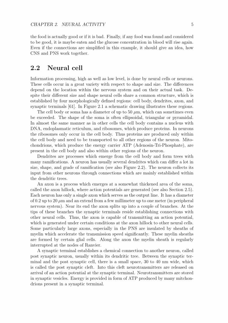
Information processing, high as well as low level, is done by neural cells or neurons.These cells occur in a great variety with respect to shape and size. The differencesdepend on the location within the nervous system and on their actual task. De-spite their different size and shape neural cells share a common structure, which isestablished by four morphologically defined regions: cell body, dendrites, axon, andsynaptic terminals [61]. In Figure 2.1 a schematic drawing illustrates these regions.
The cell body or soma has a diameter of up to 50 µm, which can sometimes evenbe exceeded. The shape of the soma is often ellipsoidal, triangular or pyramidal.In almost the same manner as in other cells the cell body contains a nucleus withDNA, endoplasmatic reticulum, and ribosomes, which produce proteins. In neuronsthe ribosomes only occur in the cell body. Thus proteins are produced only withinthe cell body and need to be transported to all other regions of the neuron. Mito-chondrions, which produce the energy carrier ATP (Adenosin-Tri-Phosphate), arepresent in the cell body and also within other regions of the neuron.
Dendrites are processes which emerge from the cell body and form trees withmany ramifications. A neuron has usually several dendrites which can differ a lot insize, shape, and grade of ramification (see also Figure 2.2). The neuron collects itsinput from other neurons through connections which are mainly established withinthe dendritic trees.
An axon is a process which emerges at a somewhat thickened area of the soma,called the axon hillock, where action potentials are generated (see also Section 2.5).Each neuron has only a single axon which serves as the output line. It has a diameterof 0.2 up to 20 µm and an extend from a few millimeter up to one meter (in peripheralnervous system). Near its end the axon splits up into a couple of branches. At thetips of these branches the synaptic terminals reside establishing connections withother neural cells. Thus, the axon is capable of transmitting an action potential,which is generated under certain conditions at the axon hillock to other neural cells.Some particularly large axons, especially in the PNS are insulated by sheaths ofmyelin which accelerate the transmission speed significantly. These myelin sheathsare formed by certain glial cells. Along the axon the myelin sheath is regularlyinterrupted at the nodes of Ranvier.
A synaptic terminal establishes a chemical connection to another neuron, calledpost synaptic neuron, usually within its dendritic tree. Between the synaptic ter-minal and the post synaptic cell, there is a small space, 30 to 40 nm wide, whichis called the post synaptic cleft. Into this cleft neurotransmitters are released onarrival of an action potential at the synaptic terminal. Neurotransmitters are storedin synaptic vesicles. Energy is provided in form of ATP produced by many mitchon-drions present in a synaptic terminal.
CHAPTER 2. NEURAL ACTIVITY 6
Dendrite
Axon
Synaptic terminals
Cell body
Axon hillock Nucleus
Figure 2.1: Schematic drawing of a basic neuron.

CHAPTER 2. NEURAL ACTIVITY 7
2.2.1 Morphological classification
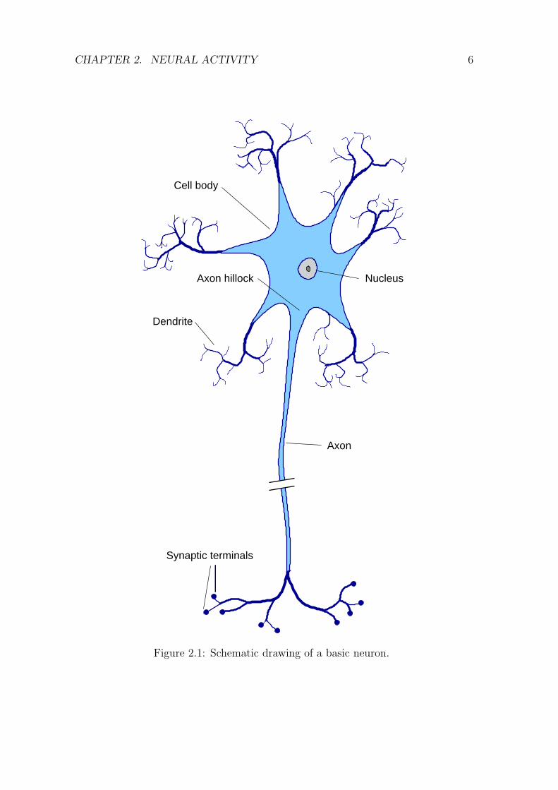
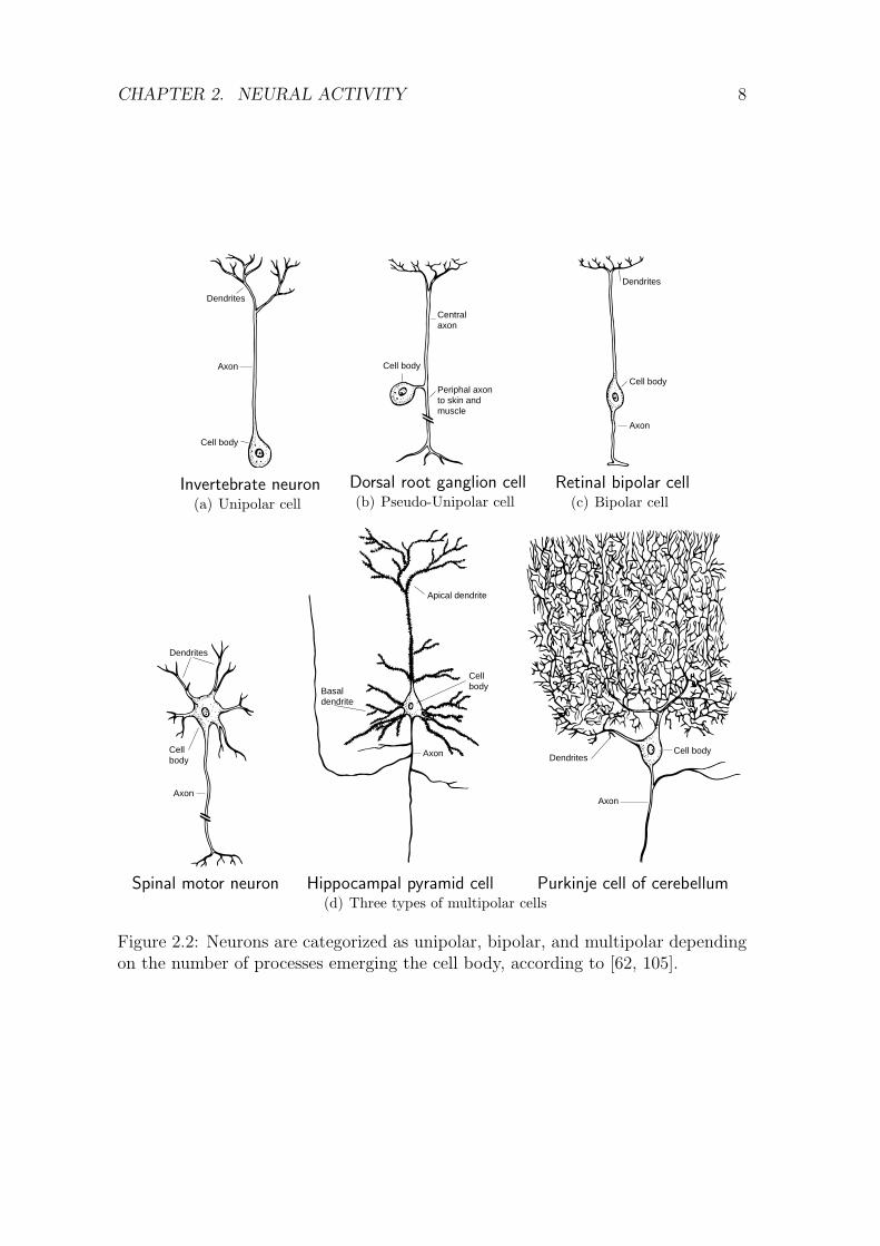
Based on the number of processes arising from their cell body neurons are classifiedinto three large groups: unipolar neurons, bipolar neurons, and multipolar neurons.Figure 2.2 shows instances of these types [61].
Unipolar neurons are characterized by a single process which emerges the cellbody and ramifies into several branches as depicted in Figure 2.2(a). One branchserves as axon and the others are dendrites. This cell type is predominant in thenervous system of invertebrates, but they do also occur in certain ganglions of ver-tebrates’ autonomic nervous system.
Bipolar neurons (Figure 2.2(c)) have an ovoid soma with two emerging processes:A dendrite, which conveys information from the periphery, and an axon which carriesinformation toward the central nervous system. Bipolar cells often have sensoryfunctionality, thus they occur e.g. in the retina or in olfactory epithelium. A specialkind of bipolar cells can be found in spinal ganglia, where they carry informationabout pressure, touch, and pain. These cells have initially two processes, but duringtheir development both processes converge and form a single process emerging thesoma, which splits into two processes. Both parts work as axons, one runs towardthe periphery (skin and muscle) and the other toward the spinal cord. These neuronsshown in Figure 2.2(b) are called pseudo-unipolar.
Multipolar neurons are preponderant in the vertebrate nervous system. Theyhave a single axon and one or more dendritic branches, emerging from all partsof the cell body. Great variations with respect to size and shape of cell bodies,and also to number and length of dendrites are found for this neuron type. Threeexamples which illustrate these variations are shown in Figure 2.2(d). The numberof contacts varies with the size of the dendritic trees. A spinal motor cell receivesinput on about 10,000 contacts (2000 on cell body, 8000 on dendrites) while havinga moderate number dendrites with a moderate extent itself. On the other hand thePurkinje cell of cerebellum with a large dendritic tree receives input of approximately150,000 contacts.
2.2.2 Functional classification
Beside the morphological classification neurons can also be classified based on theirfunctionality into three major groups, i.e. afferent, motor, and interneural neurons.
Afferent neurons carry information from the periphery into the nervous systemboth for conscious perception and for motor coordination. Motor neurons carrycommands from nervous system into the periphery. These commands coordinatemuscles and glands. Interneurons are all neurons which cannot be classified asafferent or motor neurons. They constitute the largest number of neurons andprocess information either locally or convey information from different sites withinthe nervous system.
CHAPTER 2. NEURAL ACTIVITY 8
Axon
Dendrites
Cell body
Invertebrate neuron(a) Unipolar cell
Centralaxon
Periphal axonto skin andmuscle
Cell body
Dorsal root ganglion cell(b) Pseudo-Unipolar cell
Dendrites
Axon
Cell body
Retinal bipolar cell(c) Bipolar cell
bodyCell
Axon
Dendrites
dendrite
bodyCell
Basal
Apical dendrite
Axon Dendrites
Axon
Cell body
Spinal motor neuron Hippocampal pyramid cell Purkinje cell of cerebellum(d) Three types of multipolar cells
Figure 2.2: Neurons are categorized as unipolar, bipolar, and multipolar dependingon the number of processes emerging the cell body, according to [62, 105].
CHAPTER 2. NEURAL ACTIVITY 9
2.3 Glial cells
Neurons are surrounded by glial cells, which seem not essential for information pro-cessing, but have several other tasks [61]. They support the brain structure andinsulate groups of neurons from each other. Two types of glial cells form insulatingmyelin sheaths around large axons: Oligodendrocytes in CNS and Schwann cellsin peripheral nervous system. These sheaths significantly speed up transmission ofaction potentials through long axons. Some glial cells act as scavengers, removingdebris after an injury or neural death. Another task is the buffering of K+ ion con-centration in extracellular space and to take up and remove chemical transmittersreleased by neurons during synaptic transmission. Glial cells guide migrating neu-rons during brain development and direct the outgrowth of axons. They form theblood-brain barrier and they might have nutritive functions.
2.4 Layered structure of the brain
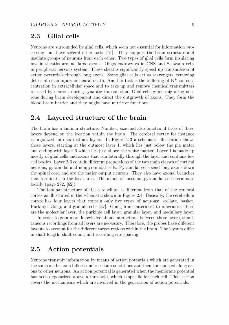
The brain has a laminar structure. Number, size and also functional tasks of theselayers depend on the location within the brain. The cerebral cortex for instanceis organized into six distinct layers. In Figure 2.3 a schematic illustration showsthese layers, starting at the outmost layer 1, which lies just below the pia materand ending with layer 6 which lies just above the white matter. Layer 1 is made upmostly of glial cells and axons that run laterally through the layer and contains fewcell bodies. Layer 2-6 contain different proportions of the two main classes of corticalneurons, pyramidal and nonpyramidal cells. Pyramidal cells send long axons downthe spinal cord and are the major output neurons. They also have axonal branchesthat terminate in the local area. The axons of most nonpyramidal cells terminatelocally (page 292, [62]).
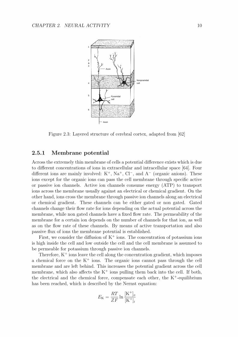
The laminar structure of the cerebellum is different from that of the cerebralcortex as illustrated in the schematic shown in Figure 2.4. Basically, the cerebellumcortex has four layers that contain only five types of neurons: stellate, basket,Purkinje, Golgi, and granule cells [37]. Going from outermost to innermost, thereare the molecular layer, the purkinje cell layer, granular layer, and medullary layer.
In order to gain more knowledge about interactions between these layers, simul-taneous recordings from all layers are necessary. Therefore, the probes have differentlayouts to account for the different target regions within the brain. The layouts differin shaft length, shaft count, and recording site spacing.
2.5 Action potentials
Neurons transmit information by means of action potentials which are generated inthe soma at the axon hillock under certain conditions and then transported along ax-ons to other neurons. An action potential is generated when the membrane potentialhas been depolarized above a threshold, which is specific for each cell. This sectioncovers the mechanisms which are involved in the generation of action potentials.
CHAPTER 2. NEURAL ACTIVITY 10
Pyramidal
cellNonpramidal
&3
2
cell
1
4
6
5
Axon
Axon
Figure 2.3: Layered structure of cerebral cortex, adapted from [62]
2.5.1 Membrane potential
Across the extremely thin membrane of cells a potential difference exists which is dueto different concentrations of ions in extracellular and intracellular space [64]. Fourdifferent ions are mainly involved: K+, Na+, Cl−, and A− (organic anions). Theseions except for the organic ions can pass the cell membrane through specific activeor passive ion channels. Active ion channels consume energy (ATP) to transportions across the membrane usually against an electrical or chemical gradient. On theother hand, ions cross the membrane through passive ion channels along an electricalor chemical gradient. These channels can be either gated or non gated. Gatedchannels change their flow rate for ions depending on the actual potential across themembrane, while non gated channels have a fixed flow rate. The permeability of themembrane for a certain ion depends on the number of channels for that ion, as wellas on the flow rate of these channels. By means of active transportation and alsopassive flux of ions the membrane potential is established.
First, we consider the diffusion of K+ ions. The concentration of potassium ionsis high inside the cell and low outside the cell and the cell membrane is assumed tobe permeable for potassium through passive ion channels.
Therefore, K+ ions leave the cell along the concentration gradient, which imposesa chemical force on the K+ ions. The organic ions cannot pass through the cellmembrane and are left behind. This increases the potential gradient across the cellmembrane, which also affects the K+ ions pulling them back into the cell. If both,the electrical and the chemical force, compensate each other, the K+-equilibriumhas been reached, which is described by the Nernst equation:
EK =RT
ZFln
[K+]o[K+]i
CHAPTER 2. NEURAL ACTIVITY 11
Figure 2.4: Layered structure of the cerebellum, in a schematic drawing of cerebel-lum [90].
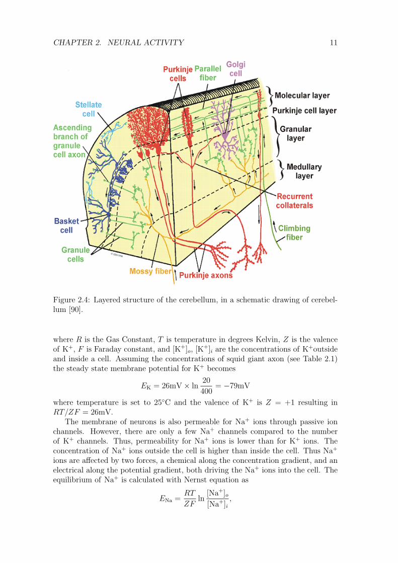
where R is the Gas Constant, T is temperature in degrees Kelvin, Z is the valenceof K+, F is Faraday constant, and [K+]o, [K+]i are the concentrations of K+outsideand inside a cell. Assuming the concentrations of squid giant axon (see Table 2.1)the steady state membrane potential for K+ becomes
EK = 26mV× ln20
400= −79mV
where temperature is set to 25C and the valence of K+ is Z = +1 resulting inRT/ZF = 26mV.
The membrane of neurons is also permeable for Na+ ions through passive ionchannels. However, there are only a few Na+ channels compared to the numberof K+ channels. Thus, permeability for Na+ ions is lower than for K+ ions. Theconcentration of Na+ ions outside the cell is higher than inside the cell. Thus Na+
ions are affected by two forces, a chemical along the concentration gradient, and anelectrical along the potential gradient, both driving the Na+ ions into the cell. Theequilibrium of Na+ is calculated with Nernst equation as
ENa =RT
ZFln
[Na+]o[Na+]i
,
CHAPTER 2. NEURAL ACTIVITY 12
Ion Cytoplasm (mM) Extracellular fluid (mM) Nernst potential (mV)K+ 400 20 -79Na+ 50 440 +55Cl− 52 560 -60A− 385 – –
Table 2.1: Distribution of the major ions across the membrane of the squid giantaxon [64].
i.e. for the squid giant axon about +55 mV given the concentrations from Table 2.1.Na+ is about 130 mV away from its equilibrium at the K+ Nernst potential of-79 mV. Thus, the electrochemical force which drives Na+ into the cell is quitestrong. The influx of Na+ into the cell is compensated by an efflux of K+ outof the cell. Note, that the permeability of the membrane to Na+ is much lowerthan the permeability to K+. Therefore the balance point shifts only slightly awayfrom the membrane potential established only by K+ ions. But a constant influxof Na+ and outflux of K+ cannot persist forever. After a while the concentrationgradients of K+ and Na+ would be flat, and the membrane potential would run low.This is prevented by an Na+-K+ pump, i.e. an active channel, which extrudes Na+
from the cell while taking in K+. Both types of ions are moved against their netelectrochemical gradients and, thus, this process needs energy, which is provided byhydrolysis of ATP.
All nerve cells have non-gated Cl− ion channels. However, since Cl− is in equi-librium at a potential of -61 mV we can ignore the contribution of Cl− ions to theresting membrane potential of nerve cells, since they do not change much.
The actual resting membrane potential depends on the interaction of two or moretypes of ions and is described by the Goldman equation:
Vm =RT
FlnPK[K+]o + PNa[Na+]o + PCl[Cl−]oPK[K+]i + PNa[Na+]i + PCl[Cl−]i
. (2.1)
Both permeability of the membrane for the specific ion and concentration inside andoutside the cell influence the resting membrane potential.
2.5.2 Action potential generation
Action potentials are generated by a change of permeability of the membrane (Hodgkin-Huxley-Model) [64]. The initial condition for an action potential is a depolarizationof the membrane potential e.g. by an excitatory synaptic potential. This depolar-ization causes some voltage gated sodium channels to open and the influx of Na+
into the cell driven by chemical and electrical forces increases. This in turn causesa further depolarization and again more voltage gated Na+ channels open. Theinflux of Na+ accelerates again. This regenerative, positive feedback cycle developsexplosively, and it leads the membrane potential toward the Na+ equilibrium poten-tial of +55 mV. However, this potential is never reached, because of the continuedK+ efflux through the K+ channels. Two mechanisms repolarize the membrane

CHAPTER 2. NEURAL ACTIVITY 13
KgNa
Repolarization
Dep
olar
izat
ion
Con
duct
ivity
(g)
potentialMembran
g
Time
Threshold
Pot
entia
l
Figure 2.5: Scheme of an action potential. The conductivity of the membrane forNa+ and K+ is denoted by gNa and gK, respectively. The conductivities change overtime triggered by an initial depolarization which must exceed a certain threshold.
and terminate the action potential. First, the continued depolarization slowly turnsoff or inactivates the voltage-gated Na+ channels. Answering to a depolarizationthe channels open fast, but a continued depolarization slowly closes the channels.Second, with a delay voltage-gated K+ channels open which increase permeabilityto K+ and therefore the efflux of K+. Figure 2.5 shows changes of the membranepotential during an action potential.
Note, that the action potential generation follows an “All or Nothing” rule [36].If the depolarization has exceeded a certain threshold, a full-fledged action potentialis generated. The grade of exceedance does not change height, length, or shape of theaction potential, at least if other parameters remain constant. After generation ofan action potential the cell can generate the next action potential after the absoluterefractory period has been expired, which is about 1 ms.
2.6 Field potentials
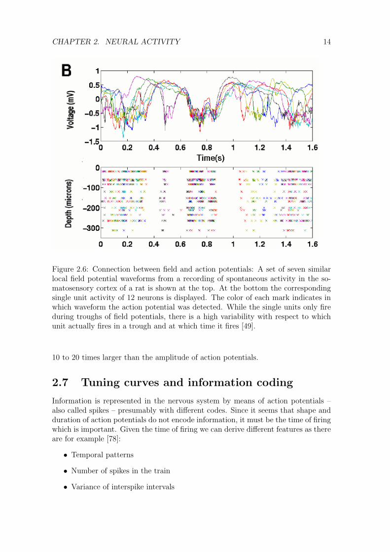
Field potentials or local field potentials (LFP) reflect almost exclusively synapticpotentials and synchronous subthreshold membrane deflections [65]. They do notseem to reflect synchronous firing of action potentials, as even similar shaped LFPshow different temporal firing patterns of neurons, which is reported in [49] andillustrated in Figure 2.6. There is no clear pattern in the recorded single unitbehaviour. A unit recording alone may give a wrong idea about the involvement ofthe cell that fires (or does not fire) in the population activity. In order to get a betterunderstanding of the interaction between field potentials and action potentials it isnecessary to study both together. This implies that the data acquisition system isable to record field and action potentials simultaneously, i.e. it must have a highbandwidth and a high analog digital conversion resolution, because the frequency offield potentials ranges from 0.5 Hz up to 80 Hz while their amplitude is a factor of
CHAPTER 2. NEURAL ACTIVITY 14
Figure 2.6: Connection between field and action potentials: A set of seven similarlocal field potential waveforms from a recording of spontaneous activity in the so-matosensory cortex of a rat is shown at the top. At the bottom the correspondingsingle unit activity of 12 neurons is displayed. The color of each mark indicates inwhich waveform the action potential was detected. While the single units only fireduring troughs of field potentials, there is a high variability with respect to whichunit actually fires in a trough and at which time it fires [49].
10 to 20 times larger than the amplitude of action potentials.
2.7 Tuning curves and information coding
Information is represented in the nervous system by means of action potentials –also called spikes – presumably with different codes. Since it seems that shape andduration of action potentials do not encode information, it must be the time of firingwhich is important. Given the time of firing we can derive different features as thereare for example [78]:
• Temporal patterns
• Number of spikes in the train
• Variance of interspike intervals
CHAPTER 2. NEURAL ACTIVITY 15
(a) (b)
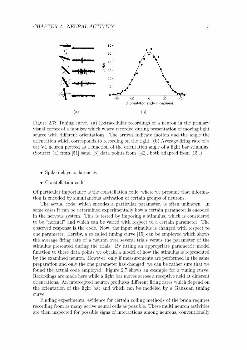
Figure 2.7: Tuning curve. (a) Extracellular recordings of a neuron in the primaryvisual cortex of a monkey which where recorded during presentation of moving lightsource with different orientations. The arrows indicate motion and the angle theorientation which corresponds to recording on the right. (b) Average firing rate of acat V1 neuron plotted as a function of the orientation angle of a light bar stimulus.(Source: (a) from [51] sand (b) data points from [42], both adapted from [15].)
• Spike delays or latencies
• Constellation code
Of particular importance is the constellation code, where we presume that informa-tion is encoded by simultaneous activation of certain groups of neurons.
The actual code, which encodes a particular parameter, is often unknown. Insome cases it can be determined experimentally how a certain parameter is encodedin the nervous system. This is tested by imposing a stimulus, which is consideredto be “normal” and which can be varied with respect to a certain parameter. Theobserved response is the code. Now, the input stimulus is changed with respect toone parameter. Hereby, a so called tuning curve [15] can be employed which showsthe average firing rate of a neuron over several trials versus the parameter of thestimulus presented during the trials. By fitting an appropriate parametric modelfunction to these data points we obtain a model of how the stimulus is representedby the examined neuron. However, only if measurements are performed in the samepreparation and only the one parameter has changed, we can be rather sure that wefound the actual code employed. Figure 2.7 shows an example for a tuning curve.Recordings are made here while a light bar moves across a receptive field at differentorientations. An intercepted neuron produces different firing rates which depend onthe orientation of the light bar and which can be modeled by a Gaussian tuningcurve.
Finding experimental evidence for certain coding methods of the brain requiresrecording from as many active neural cells as possible. These multi neuron activitiesare then inspected for possible signs of interactions among neurons, conventionally

CHAPTER 2. NEURAL ACTIVITY 16
by use of cross-correlation techniques, usually applied to pairs or triplets of neu-rons [35]. General techniques for measuring neural activity and the particular designof the VSAMUEL probes are described in the next chapter.

Chapter 3
Neural signal acquisition
The neural activity within a living brain results in different interceptable signals.These can be measured by various means, which differ with respect to spatial reso-lution, time resolution, and whether they are invasive or non-invasive.
Electroencephalogram (EEG) is a non-invasive method which has a time resolu-tion of up to 70 Hz and a rather low spatial resolution. Electrodes with diametersranging from 0.4 cm to 1 cm are attached to the scalp with special pastes and capsor nets which hold them in place. In standard clinical practice an EEG is recordedwith about 20 electrodes arranged using the International 10-20 System [58]. How-ever, for research purposes also settings with about 100 or even more electrodes areused. One electrode records the electric field potentials generated in tissue that con-tains approximately 10 million to one billion neurons [85]. Therefore, this methodgives an overview of neural activity in the complete brain. Despite the low spatialresolution (about 1 cm3) patterns which can be found in EEG recordings indicatea certain state of consciousness. For example the state of deep sleep is linked withlarge amplitude oscillations in the so-called delta band (about 1-4 Hz). Further-more, by analyzing EEG data it is possible to identify distinct sleep stage, depth ofanesthesia, or epileptic seizures. EEG is also used for the determination of cerebraldeath [50].
The major limitation for recording EEG signals is the distance from electrodeon the scalp to the underlying neural tissue which ranges between 2 and 3 cm [91].This barrier which consists of skin, bone, and liquor acts like a low-pass filter. Aninvasive variant of the EEG, which avoids this limitation, is the Electrocorticogram(ECoG) where recording electrodes are placed directly onto the cortex. This methodachieves a much finer spatial resolution on the order of 1 mm and also allows therecording of higher-frequency content (10-200 Hz) [91]. Electrodes with about 4 mmdiameter arranged in grids or strips on a foil with a spacing of 1 cm between theelectrodes are implanted directly onto the cortex. An Electrocorticogram is forexample recorded from epileptic patients in order to determine the cortical regionthat generates epileptic seizures [66].
Local field potentials (LFPs) are obtained as the low frequency (up to about300 Hz without DC) component of extracellular voltage measurement with microelectrodes inserted into the cortex. There are various types of micro electrodesincluding e.g. micro wires, micro pipettes, or fork shaped silicon. Their recording
17
CHAPTER 3. NEURAL SIGNAL ACQUISITION 18
Electroencephalogram (EEG) 3 cm
Electrocorticogram (ECoG) 0.5 cm
Local Field Potential (LFP) 1-3 mm
Multi Unit Action Potential (MUA) 0.4 mm
Single Unit Action Potential (SUA) 0.2 mm
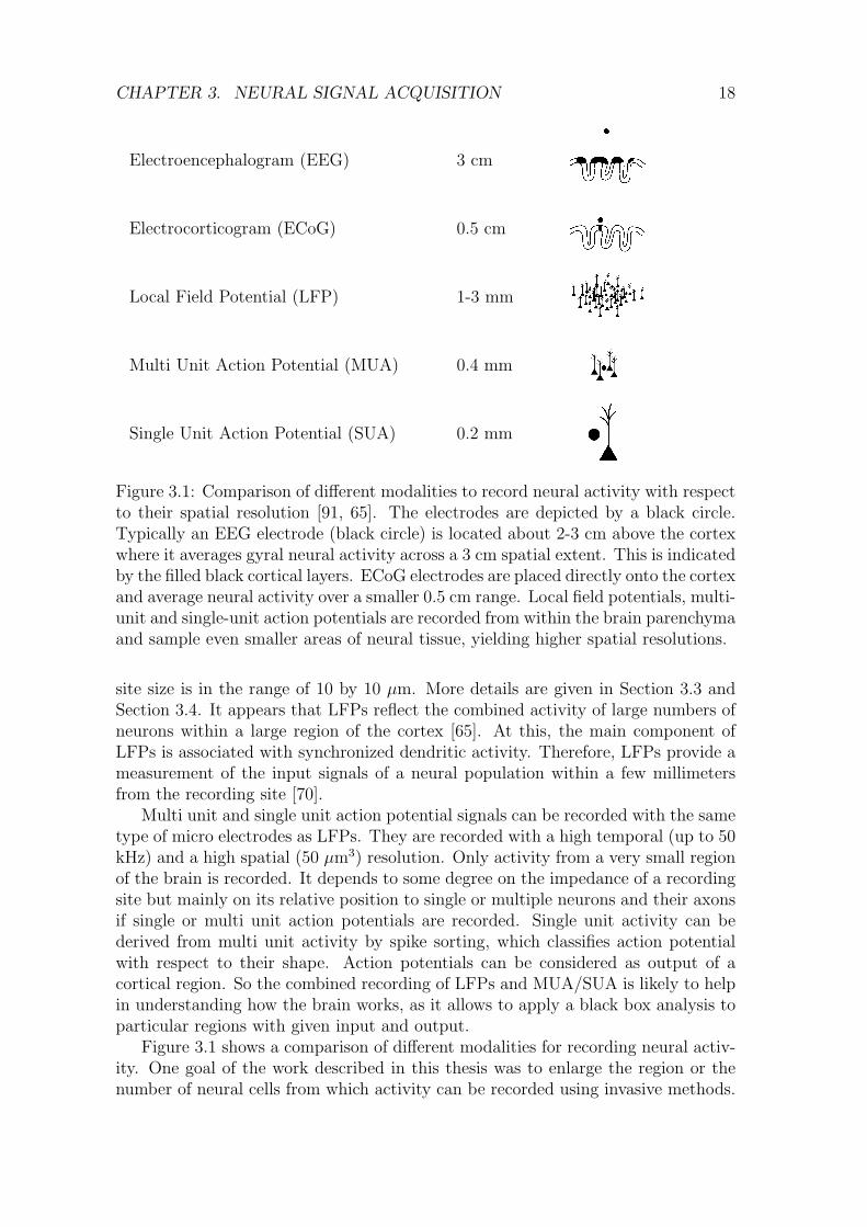
Figure 3.1: Comparison of different modalities to record neural activity with respectto their spatial resolution [91, 65]. The electrodes are depicted by a black circle.Typically an EEG electrode (black circle) is located about 2-3 cm above the cortexwhere it averages gyral neural activity across a 3 cm spatial extent. This is indicatedby the filled black cortical layers. ECoG electrodes are placed directly onto the cortexand average neural activity over a smaller 0.5 cm range. Local field potentials, multi-unit and single-unit action potentials are recorded from within the brain parenchymaand sample even smaller areas of neural tissue, yielding higher spatial resolutions.
site size is in the range of 10 by 10 µm. More details are given in Section 3.3 andSection 3.4. It appears that LFPs reflect the combined activity of large numbers ofneurons within a large region of the cortex [65]. At this, the main component ofLFPs is associated with synchronized dendritic activity. Therefore, LFPs provide ameasurement of the input signals of a neural population within a few millimetersfrom the recording site [70].
Multi unit and single unit action potential signals can be recorded with the sametype of micro electrodes as LFPs. They are recorded with a high temporal (up to 50kHz) and a high spatial (50 µm3) resolution. Only activity from a very small regionof the brain is recorded. It depends to some degree on the impedance of a recordingsite but mainly on its relative position to single or multiple neurons and their axonsif single or multi unit action potentials are recorded. Single unit activity can bederived from multi unit activity by spike sorting, which classifies action potentialwith respect to their shape. Action potentials can be considered as output of acortical region. So the combined recording of LFPs and MUA/SUA is likely to helpin understanding how the brain works, as it allows to apply a black box analysis toparticular regions with given input and output.
Figure 3.1 shows a comparison of different modalities for recording neural activ-ity. One goal of the work described in this thesis was to enlarge the region or thenumber of neural cells from which activity can be recorded using invasive methods.
CHAPTER 3. NEURAL SIGNAL ACQUISITION 19
Iron -440 mVLead -126 mVCopper +337 mVPlatinum +1190 mV
Table 3.1: Electrode potentials for some metals
R
s
d
d
hcE
R
C
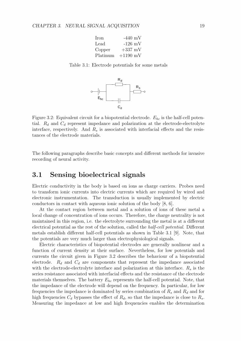
Figure 3.2: Equivalent circuit for a biopotential electrode. Ehc is the half-cell poten-tial. Rd and Cd represent impedance and polarization at the electrode-electrolyteinterface, respectively. And Rs is associated with interfacial effects and the resis-tances of the electrode materials.
The following paragraphs describe basic concepts and different methods for invasiverecording of neural activity.
3.1 Sensing bioelectrical signals
Electric conductivity in the body is based on ions as charge carriers. Probes needto transform ionic currents into electric currents which are required by wired andelectronic instrumentation. The transduction is usually implemented by electricconductors in contact with aqueous ionic solution of the body [8, 6].
At the contact region between metal and a solution of ions of these metal alocal change of concentration of ions occurs. Therefore, the charge neutrality is notmaintained in this region, i.e. the electrolyte surrounding the metal is at a differentelectrical potential as the rest of the solution, called the half-cell potential. Differentmetals establish different half-cell potentials as shown in Table 3.1 [9]. Note, thatthe potentials are very much larger than electrophysiological signals.
Electric characteristics of biopotential electrodes are generally nonlinear and afunction of current density at their surface. Nevertheless, for low potentials andcurrents the circuit given in Figure 3.2 describes the behaviour of a biopotentialelectrode. Rd and Cd are components that represent the impedance associatedwith the electrode-electrolyte interface and polarization at this interface. Rs is theseries resistance associated with interfacial effects and the resistance of the electrodematerials themselves. The battery Ehc represents the half-cell potential. Note, thatthe impedance of the electrode will depend on the frequency. In particular, for lowfrequencies the impedance is dominated by series combination of Rs and Rd and forhigh frequencies Cd bypasses the effect of Rd, so that the impedance is close to Rs.Measuring the impedance at low and high frequencies enables the determination
CHAPTER 3. NEURAL SIGNAL ACQUISITION 20
of the parameters of the components of the circuit. However, electrode impedanceis affected by a change in surface area due to roughness and radius of curvature.Furthermore the impedance is affected by contamination of the electrode surface.
3.2 Extracellular potentials
The generation of extracellular potentials can be completely derived from well knownbiophysical principles of neural excitability [84, 48]. Ionic currents which come alongwith action potentials and subthreshold activity flow in closed loops. They enterthe neuron at current sink regions, propagate through the cytosolic medium, leaveit at current source regions, and return to the sink points through the extracellularspace. Spatio-temporal patterns of extracellular voltages appear as a result of thisreturn current [12].
Figure 3.3 shows an extracellular recording setup with a single microelectrode.The electrode is moved toward the axon until the gap resistance increases to about20 kΩ. Then the electrode in an in vitro setup is placed about 5 µm away fromthe axon, as determined by visual inspection in [12]. With this gap resistance it ispossible to obtain recordings from the soma. Note, that an appropriate resistancebetween reference electrode and microelectrode is crucial to obtain recordings. Thiscorroborates the evidence for extracellular current pathways. However, if measure-ments are performed with multisite electrodes, it is impossible to place each singlerecording site as close as 5 µm to the soma or axon of a neural cell. But the reducedextracellular space, which is due to the compact arrangement of neurons and glialcells, increases the effective resistance through which extracellular currents circulate.Thus, potential differences in the order of 100 µV can be detected, even withoutplacing the recordings sites very close to neurons [12]. Furthermore, the high den-sity of neurons also maximizes the probability of an electrode being quite close to asufficiently intense current source or sink.
3.3 Probes for intracavitary or intratissue record-
ings
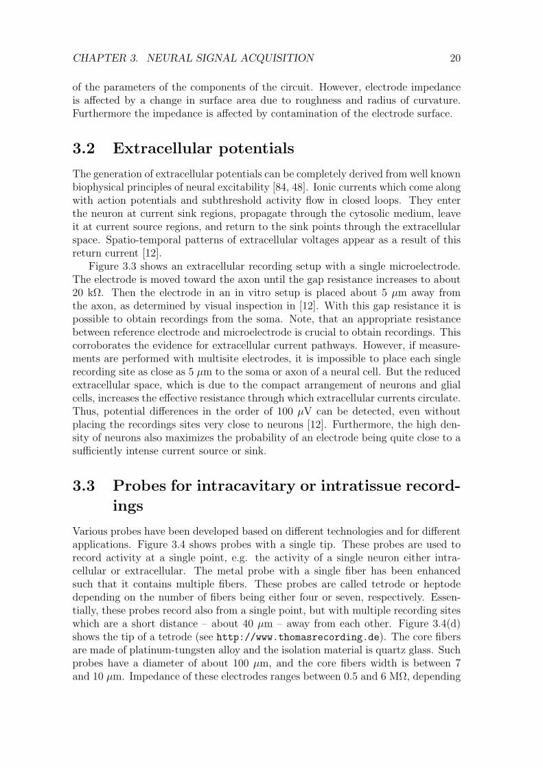
Various probes have been developed based on different technologies and for differentapplications. Figure 3.4 shows probes with a single tip. These probes are used torecord activity at a single point, e.g. the activity of a single neuron either intra-cellular or extracellular. The metal probe with a single fiber has been enhancedsuch that it contains multiple fibers. These probes are called tetrode or heptodedepending on the number of fibers being either four or seven, respectively. Essen-tially, these probes record also from a single point, but with multiple recording siteswhich are a short distance – about 40 µm – away from each other. Figure 3.4(d)shows the tip of a tetrode (see http://www.thomasrecording.de). The core fibersare made of platinum-tungsten alloy and the isolation material is quartz glass. Suchprobes have a diameter of about 100 µm, and the core fibers width is between 7and 10 µm. Impedance of these electrodes ranges between 0.5 and 6 MΩ, depending

CHAPTER 3. NEURAL SIGNAL ACQUISITION 21
Gap resistance
Axon
electrodeReference
~5 micrometer
about 20 kOhm
Soma
Figure 3.3: Extracellular recording and gap resistance
on the manufacturing process, in particular the grinding angle which ranges from15 to 17. The advantage of multiple recording sites close to each other is, thatthe performance of analysis tasks like e.g. spike sorting (see Section 5.4) can beincreased [40].
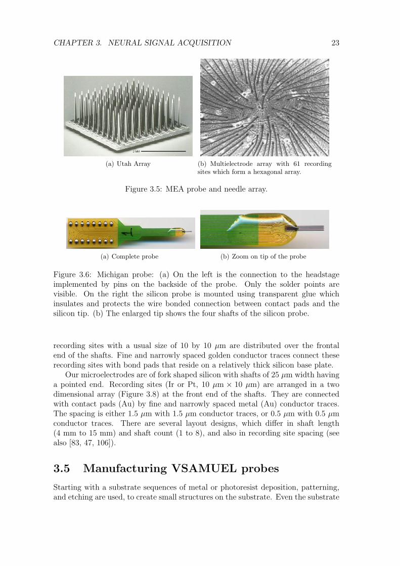
Another class of probes has recording sites which are arranged as a two dimen-sional array. These probes differ in size, shape, and material and also in field ofapplication. One example shown in Figure 3.5(a) is an array of microelectrodesdeveloped at Moran Laboratories in the Department of Bioengineering at the Uni-versity of Utah. 100 silicon spikes, each 1.5 mm long, are arranged in a regulargrid on a 4 mm by 4 mm base. Each spike has one recording site and the arrayis used to record from cortex. Another example are the probes developed and pro-duced by Center for Neural Communication Technology at University of Michigan asshown in Figure 3.6. They consist of fork shaped silicon with recording sites linearlyarranged on the shafts. Number and length of shafts and also spacing and arrange-ment of recording sites can vary. All aforementioned probes are used to recordfrom in vivo or in vitro preparations of nervous tissue. Another technique whichrequires a special type of probes is the recording from cultured neuron which growin dish containing transparent conductors and recording sites (indium-tin oxide) ona glass substrate. This kind of probe is called multielectrode array (MEA) andFigure 3.5(b) shows an example MEA with 61 recording sites forming a hexagonalarray (see http://www.neuro.gatech.edu/potter/netinadish.html).
After this overview the next paragraphs will describe the microelectrodes devel-oped within the project VSAMUEL in detail.
CHAPTER 3. NEURAL SIGNAL ACQUISITION 22
Tip
Metal
Glass
(a) Metal
Tip
Metal electrode
ElectrolyteLead wire
Cap
(b) Micropipette
Glass
Insulation
Tip
Metal film
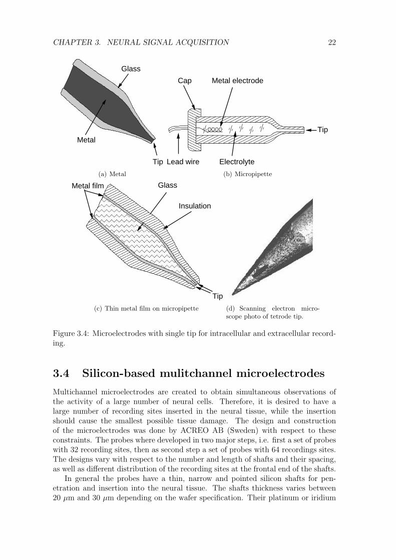
(c) Thin metal film on micropipette (d) Scanning electron micro-scope photo of tetrode tip.
Figure 3.4: Microelectrodes with single tip for intracellular and extracellular record-ing.
3.4 Silicon-based mulitchannel microelectrodes
Multichannel microelectrodes are created to obtain simultaneous observations ofthe activity of a large number of neural cells. Therefore, it is desired to have alarge number of recording sites inserted in the neural tissue, while the insertionshould cause the smallest possible tissue damage. The design and constructionof the microelectrodes was done by ACREO AB (Sweden) with respect to theseconstraints. The probes where developed in two major steps, i.e. first a set of probeswith 32 recording sites, then as second step a set of probes with 64 recordings sites.The designs vary with respect to the number and length of shafts and their spacing,as well as different distribution of the recording sites at the frontal end of the shafts.
In general the probes have a thin, narrow and pointed silicon shafts for pen-etration and insertion into the neural tissue. The shafts thickness varies between20 µm and 30 µm depending on the wafer specification. Their platinum or iridium
CHAPTER 3. NEURAL SIGNAL ACQUISITION 23
(a) Utah Array (b) Multielectrode array with 61 recordingsites which form a hexagonal array.
Figure 3.5: MEA probe and needle array.
(a) Complete probe (b) Zoom on tip of the probe
Figure 3.6: Michigan probe: (a) On the left is the connection to the headstageimplemented by pins on the backside of the probe. Only the solder points arevisible. On the right the silicon probe is mounted using transparent glue whichinsulates and protects the wire bonded connection between contact pads and thesilicon tip. (b) The enlarged tip shows the four shafts of the silicon probe.
recording sites with a usual size of 10 by 10 µm are distributed over the frontalend of the shafts. Fine and narrowly spaced golden conductor traces connect theserecording sites with bond pads that reside on a relatively thick silicon base plate.
Our microelectrodes are of fork shaped silicon with shafts of 25 µm width havinga pointed end. Recording sites (Ir or Pt, 10 µm × 10 µm) are arranged in a twodimensional array (Figure 3.8) at the front end of the shafts. They are connectedwith contact pads (Au) by fine and narrowly spaced metal (Au) conductor traces.The spacing is either 1.5 µm with 1.5 µm conductor traces, or 0.5 µm with 0.5 µmconductor traces. There are several layout designs, which differ in shaft length(4 mm to 15 mm) and shaft count (1 to 8), and also in recording site spacing (seealso [83, 47, 106]).
3.5 Manufacturing VSAMUEL probes
Starting with a substrate sequences of metal or photoresist deposition, patterning,and etching are used, to create small structures on the substrate. Even the substrate

CHAPTER 3. NEURAL SIGNAL ACQUISITION 24
Probe Site Count Region Application Referenceintra extra
Capillary electrodes 1 single cells√ √
[8]Tungsten wire 1 single cells
√ √[89]
Stereotrode,Tetrode, Heptode
2, 4, 7 multiple cells –√
[89]
Needle array ca. 100 many cells 4 ×4mm
–√
[10]
Flat array ca. 100 –√
[38]Fork shaped silicon 32, 64, 96 2× 2mm –
√[74]
(a) Four shafts with 16 electrodes each (b) Close up of one of the shafts
Figure 3.7: Scanning electron micrographs of a 64-site neural probe, model E4
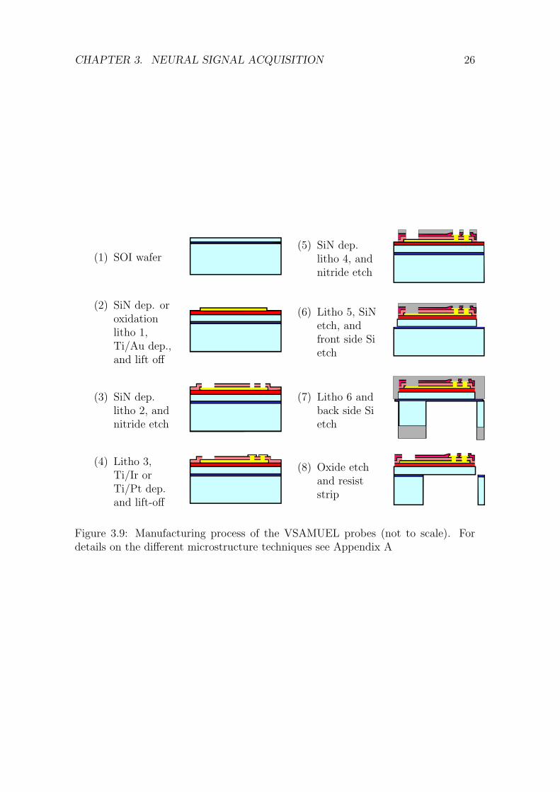
itself can be shaped. The manufacturing of the VSAMUEL probes incorporatesseveral microstructuring techniques. Some of the important techniques used aredescribed in the Appendix. An overview of the manufacturing process is givenby Figure 3.9. According to [83] the single steps are:
(1) Probes are manufactured on silicon-on-insulator (SOI) substrate. Buried insidethe substrate is an oxide layer which is supposed to stop the two deep etchingprocesses, which are applied as the final process steps (Step 7 and 8).
(2) A first isolation layer is deposited, either in form of a thermally grown oxidefilm or alternatively as a PECVD (Plasma Enhanced Chemical Vapor Deposi-tion) silicon nitride film. Afterwards the conductor traces which consist of Tior Au are created on top of this layer (e-beam evaporation, patterned with aphotoresist lift-off process).
(3) The conductor traces are covered by another silicon nitride layer, which in turnis opened down to the Au/Ti layer by reactive ion etching (RIE) through a resistmask. At these openings electrode sites and contact pads will arise later in theprocess.
(4) Electrode sites are formed with Ti/Pt (e-beam evaporation, patterned with aphotoresist lift-off process)
CHAPTER 3. NEURAL SIGNAL ACQUISITION 25
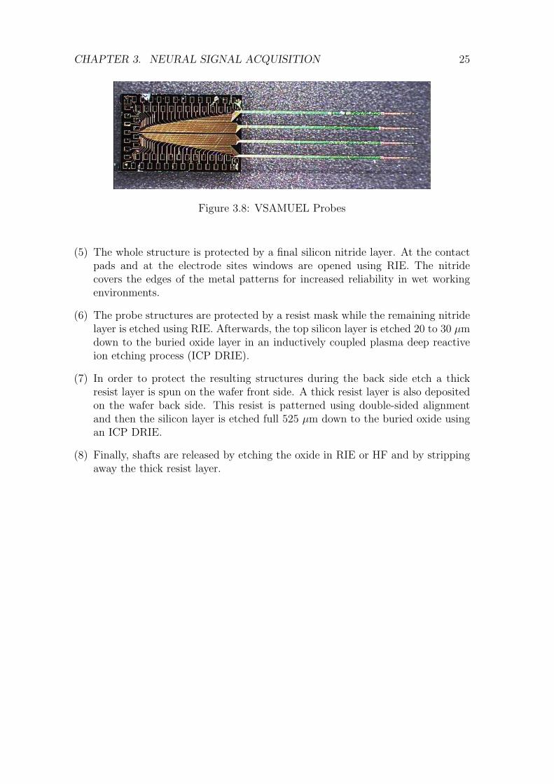
Figure 3.8: VSAMUEL Probes
(5) The whole structure is protected by a final silicon nitride layer. At the contactpads and at the electrode sites windows are opened using RIE. The nitridecovers the edges of the metal patterns for increased reliability in wet workingenvironments.
(6) The probe structures are protected by a resist mask while the remaining nitridelayer is etched using RIE. Afterwards, the top silicon layer is etched 20 to 30 µmdown to the buried oxide layer in an inductively coupled plasma deep reactiveion etching process (ICP DRIE).
(7) In order to protect the resulting structures during the back side etch a thickresist layer is spun on the wafer front side. A thick resist layer is also depositedon the wafer back side. This resist is patterned using double-sided alignmentand then the silicon layer is etched full 525 µm down to the buried oxide usingan ICP DRIE.
(8) Finally, shafts are released by etching the oxide in RIE or HF and by strippingaway the thick resist layer.
CHAPTER 3. NEURAL SIGNAL ACQUISITION 26
(1) SOI wafer(5) SiN dep.
litho 4, andnitride etch
(2) SiN dep. oroxidationlitho 1,Ti/Au dep.,and lift off
(6) Litho 5, SiNetch, andfront side Sietch
(3) SiN dep.litho 2, andnitride etch
(7) Litho 6 andback side Sietch
(4) Litho 3,Ti/Ir orTi/Pt dep.and lift-off
(8) Oxide etchand resiststrip
Figure 3.9: Manufacturing process of the VSAMUEL probes (not to scale). Fordetails on the different microstructure techniques see Appendix A

Chapter 4
Signal processing
An essential part of the VSAMUEL data acquisition system is the signal processingmodule. Acquired data must be analyzed automatically by appropriate algorithmsin order to extract the desired information. Digital signal processing is used by thedata acquisition system to perform the following tasks:
• Separate action potentials and field potentials
• Remove noise
• Detect action potentials
• Classify action potentials
The data acquisition system is able to perform some of these tasks during record-ing in real time in order to provide direct feedback about signal quality. In particularthe results of the first three tasks are relevant for a first ad hoc decision whether arecording setup yields useful signals. The classification of action potentials is a taskthat could also be performed online. However, not all methods for spike sorting canbe applied online as for example a principal component analysis requires that thedata is fully available.
The following paragraphs give an overview about the employed signal processingmethods [33]. In particular implementation of the wavelet transformation using thelifting scheme is described.
4.1 Digital filter
Digital filters are usually instances of linear time invariant (LTI) systems which areused to select, attenuate, or amplify certain frequency components of an input signals(n). The result is an output signal g(n). In general an LTI system can be describedby a linear difference equation with constant coefficients
N∑k=0
akg(n− k) =M∑k=0
bks(n− k) (4.1)
27
CHAPTER 4. SIGNAL PROCESSING 28
Transitionzone StopbandPassband
f
|H(f)|
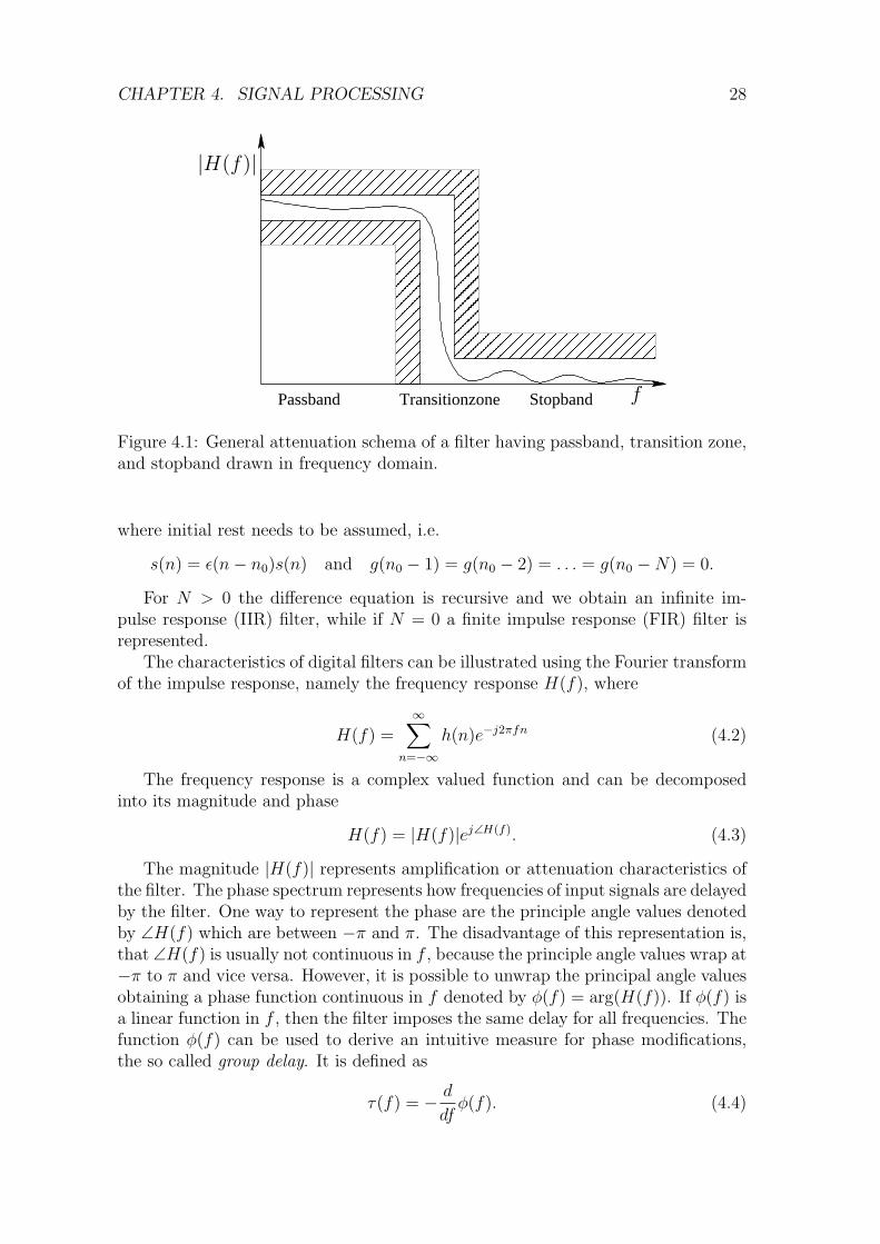
Figure 4.1: General attenuation schema of a filter having passband, transition zone,and stopband drawn in frequency domain.
where initial rest needs to be assumed, i.e.
s(n) = ε(n− n0)s(n) and g(n0 − 1) = g(n0 − 2) = . . . = g(n0 −N) = 0.
For N > 0 the difference equation is recursive and we obtain an infinite im-pulse response (IIR) filter, while if N = 0 a finite impulse response (FIR) filter isrepresented.
The characteristics of digital filters can be illustrated using the Fourier transformof the impulse response, namely the frequency response H(f), where
H(f) =∞∑
n=−∞
h(n)e−j2πfn (4.2)
The frequency response is a complex valued function and can be decomposedinto its magnitude and phase
H(f) = |H(f)|ej∠H(f). (4.3)
The magnitude |H(f)| represents amplification or attenuation characteristics ofthe filter. The phase spectrum represents how frequencies of input signals are delayedby the filter. One way to represent the phase are the principle angle values denotedby ∠H(f) which are between −π and π. The disadvantage of this representation is,that ∠H(f) is usually not continuous in f , because the principle angle values wrap at−π to π and vice versa. However, it is possible to unwrap the principal angle valuesobtaining a phase function continuous in f denoted by φ(f) = arg(H(f)). If φ(f) isa linear function in f , then the filter imposes the same delay for all frequencies. Thefunction φ(f) can be used to derive an intuitive measure for phase modifications,the so called group delay. It is defined as
τ(f) = − d
dfφ(f). (4.4)
CHAPTER 4. SIGNAL PROCESSING 29
A system shifts a signal of frequency f by τ(f) samples. The group delay is constantfor a filter with linear phase. Deviations of the group delay from a constant indicatethe degree of nonlinearity of the phase. Note, that a filter with constant group delaypreserves the shape of the original signal better than a filter with non constant groupdelay. The following paragraph will illustrate this with an example.
4.1.1 FIR and IIR filter
An FIR filter h(n) with M + 1 taps is applied on a signal s(n) by computing theconvolution as
g(n) = h(n) ∗ s(n) =M∑k=0
h(k)s(n− k) (4.5)
This FIR filter is causal, i.e. h(n) = 0, n < 0. The result g(n) does not dependon values s(k) where k > n. Thus, the computation involves only signal values fromthe past, and no values from the future. In an online processing system an FIR filtermust be causal to be applied. As the signal s(n) is usually not completely available,it is processed in segments. After processing a segment the filter keeps an internalstate needed to process the following segment correctly.
An FIR filter has linear phase and constant group delay if its impulse responseis symmetric:
h(M − n) = ±h(n), (M even). (4.6)
This condition is used in the Parks-McClellan algorithm [54, 87] for FIR filter de-sign which computes linear phase FIR filter for given attenuation constraints. Thealgorithm was used to compute the coefficients of the FIR filter in the examplein the paragraph below. As a rule of thumb the number of taps for the FIR fil-ter increases with stronger constraints on the width of the transition zone and themaximal allowed error in passband and stopband.
IIR filter often have only a few coefficients bk and ak which are non zero comparedto FIR filter which satisfy the same passband, transition, and stopband constraints.Thus the computational cost of FIR filters is usually higher than the computationalcost of a corresponding IIR filter. This advantage of IIR filter goes with the dis-advantage of being possibly unstable. In fact, instability can be caused just byquantization effects which occur when the IIR filter is implemented e.g. in fixedpoint 16 bit resolution.
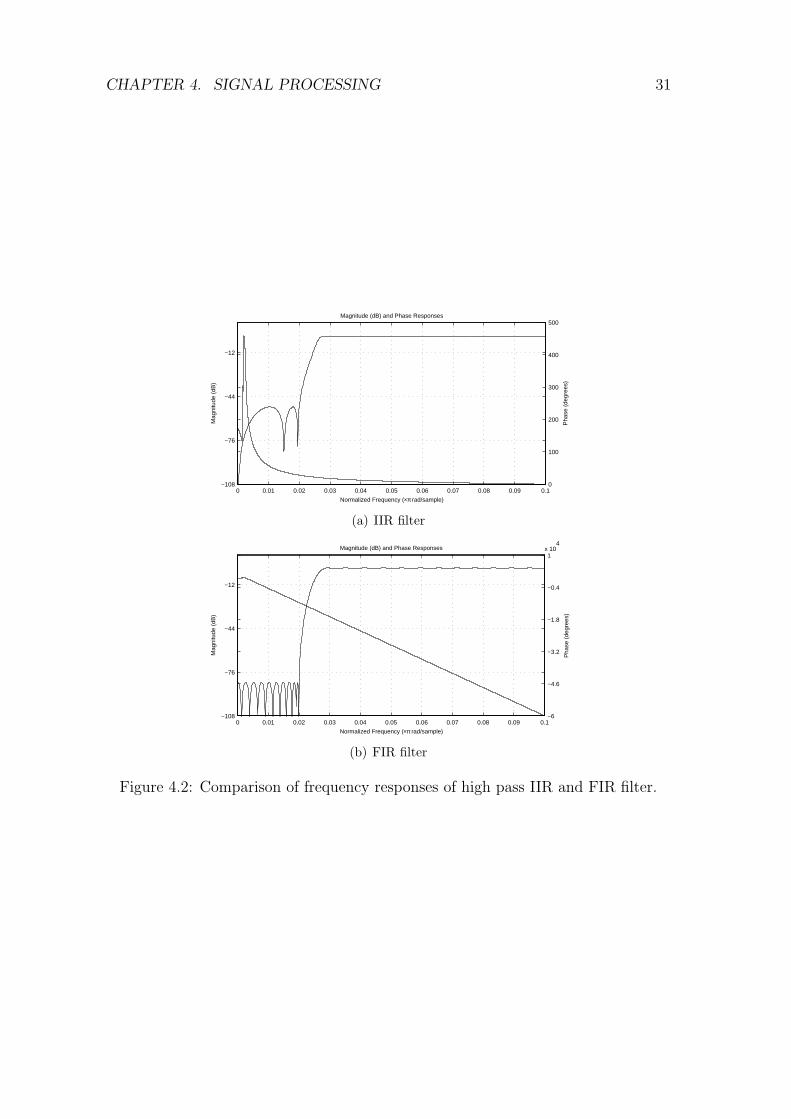
The example in Figure 4.2 and Figure 4.3 illustrates the differences between anFIR filter hFIR and an IIR filter hIIR with similar constraints. The test signal, asuperposition of sine waves with 80 Hz, 1 kHz, and 5 kHz, is defined as:
s(t) = sin(80 2πt) +1
2sin(1000 2πt) +
1
10sin(5000 2πt). (4.7)
This test signal is sampled at 50 kHz for one second yielding the time discrete func-tion s(n). Two digital high pass filters, i.e. hFIR and hIIR are designed such thatthey remove the 80 Hz sine wave from s(n). The stopband ends at 500 Hz andthe passband starts at 700 Hz. The frequencies 500 Hz and 700 Hz correspondto normalized frequency values 0.020 and 0.028, which are used for the frequency
CHAPTER 4. SIGNAL PROCESSING 30
axis in Figure 4.2. The FIR filter is designed using the Parks-McClellan algorithmwhich uses the Remez exchange algorithm and Chebyshev approximation theory todesign a filter that fits optimally to the desired frequency response, in the sensethat it minimizes the maximum error. The IIR filter hIIR is an order 30 Butter-worth filter [93], which are in general characterized by a magnitude response thatis maximally flat in the passband and monotonic overall. Butterworth filter havea more linear phase response in the passband than the Chebyshev Type I/TypeII and elliptic filters [103]. The magnitudes of the impulse responses for IIR andFIR filter are quite similar. The phase responses on the other hand are different.While the FIR filter has a linear phase with constant group delay of 343 samples,the IIR filter has a non-linear phase response. This translates into a group delay forthe passband which starts around 80 samples at 700 Hz decaying to less than onesample at 4575 Hz.
Figure 4.3 shows a closeup, i.e. the first 40 ms of the results of filtering s(n) withIIR and FIR filter hIIR and hFIR. At the top of both plots the original sequences(n) is drawn with the delay of the respective filter. Below the results gIIR and gFIRis a plot of the expected result:
g(t) =1
2sin(1000 2πt) +
1
10sin(5000 2πt) = s(t)− sin(80 2πt). (4.8)
This and the plot of the difference between actual and expected results at the bot-tom allows a visual comparison of both. As a consequence of the non-linear phaseresponse, the shape of gIIR shows more distortion than gFIR which is quite close tothe expected result.
The chosen example is similar to the task of separating local field potentials fromaction potentials. The problem with IIR filter is that it is likely to change the shapeof the action potentials. This must be avoided, since the shape of an action potentialis significant for its classification. The FIR filter nicely preserves the shape but ithas a high computational cost due to its length. Therefore, both are not well suitedto separate LFPs and APs in real time when recording at 50 kHz on 128 channels.A suitable alternative is a high pass filter implemented by means of a wavelet filterbank, which will be described in the following paragraphs.
4.2 Wavelet Transformation
In this section a short introduction into wavelets and the wavelet transform is given.As W. Sweldens indicates in [95] it is hard to give the definition of a ”wavelet”, butthey could be vaguely described with the following sentence:
”Wavelets are building blocks that can quickly decorrelate data.”
This sentence reflects three of the main features of wavelets. First, we can see themas building blocks for general data sets. More precisely, an arbitrary set of data canbe represented by a linear combination of wavelets. And even more precisely, if wedenote wavelets by ψj and the coefficients by dj, a general function s can be writtenas:
s =∑j
djψj
CHAPTER 4. SIGNAL PROCESSING 31
0 0.01 0.02 0.03 0.04 0.05 0.06 0.07 0.08 0.09 0.1−108
−76
−44
−12
Normalized Frequency (×π rad/sample)
Mag
nitu
de (
dB)
Magnitude (dB) and Phase Responses
0
100
200
300
400
500
Pha
se (
degr
ees)
(a) IIR filter
0 0.01 0.02 0.03 0.04 0.05 0.06 0.07 0.08 0.09 0.1−108
−76
−44
−12
Normalized Frequency (×π rad/sample)
Mag
nitu
de (
dB)
Magnitude (dB) and Phase Responses
−6
−4.6
−3.2
−1.8
−0.4
1x 10
4
Pha
se (
degr
ees)
(b) FIR filter
Figure 4.2: Comparison of frequency responses of high pass IIR and FIR filter.

CHAPTER 4. SIGNAL PROCESSING 32
0 0.005 0.01 0.015 0.02 0.025 0.03 0.035 0.04
Original signal
Filtered signal
Expected signal
Difference of filtered and expected signal
time [s]
(a) IIR filter
0 0.005 0.01 0.015 0.02 0.025 0.03 0.035 0.04
Original signal
Filtered signal
Expected signal
Difference of filtered and expected signal
time [s]
(b) FIR filter
Figure 4.3: Result of applying IIR and FIR high pass filter to a superposition ofsine waves.
CHAPTER 4. SIGNAL PROCESSING 33
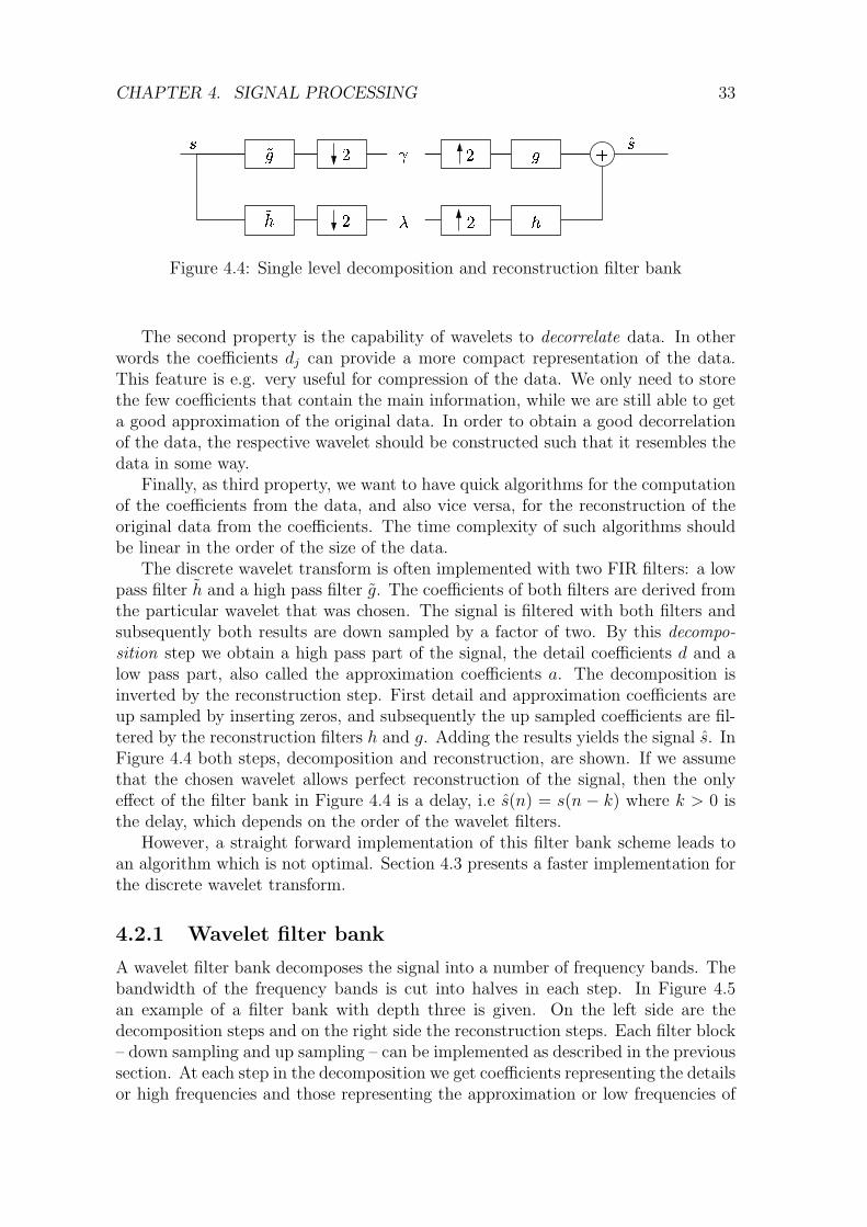
Figure 4.4: Single level decomposition and reconstruction filter bank
The second property is the capability of wavelets to decorrelate data. In otherwords the coefficients dj can provide a more compact representation of the data.This feature is e.g. very useful for compression of the data. We only need to storethe few coefficients that contain the main information, while we are still able to geta good approximation of the original data. In order to obtain a good decorrelationof the data, the respective wavelet should be constructed such that it resembles thedata in some way.
Finally, as third property, we want to have quick algorithms for the computationof the coefficients from the data, and also vice versa, for the reconstruction of theoriginal data from the coefficients. The time complexity of such algorithms shouldbe linear in the order of the size of the data.
The discrete wavelet transform is often implemented with two FIR filters: a lowpass filter h and a high pass filter g. The coefficients of both filters are derived fromthe particular wavelet that was chosen. The signal is filtered with both filters andsubsequently both results are down sampled by a factor of two. By this decompo-sition step we obtain a high pass part of the signal, the detail coefficients d and alow pass part, also called the approximation coefficients a. The decomposition isinverted by the reconstruction step. First detail and approximation coefficients areup sampled by inserting zeros, and subsequently the up sampled coefficients are fil-tered by the reconstruction filters h and g. Adding the results yields the signal s. InFigure 4.4 both steps, decomposition and reconstruction, are shown. If we assumethat the chosen wavelet allows perfect reconstruction of the signal, then the onlyeffect of the filter bank in Figure 4.4 is a delay, i.e s(n) = s(n − k) where k > 0 isthe delay, which depends on the order of the wavelet filters.
However, a straight forward implementation of this filter bank scheme leads toan algorithm which is not optimal. Section 4.3 presents a faster implementation forthe discrete wavelet transform.
4.2.1 Wavelet filter bank
A wavelet filter bank decomposes the signal into a number of frequency bands. Thebandwidth of the frequency bands is cut into halves in each step. In Figure 4.5an example of a filter bank with depth three is given. On the left side are thedecomposition steps and on the right side the reconstruction steps. Each filter block– down sampling and up sampling – can be implemented as described in the previoussection. At each step in the decomposition we get coefficients representing the detailsor high frequencies and those representing the approximation or low frequencies of

CHAPTER 4. SIGNAL PROCESSING 34
2g
2h g
2h
2g
2h
γ1
γ2
γ3
λ3
2
2g
2hZ−2l
Z−4l2g
2h
2g
2h
Figure 4.5: Wavelet filter bank of depth three
0 0.005 0.01 0.015 0.02 0.025 0.03 0.035 0.04
Original signal
Filtered signal
Expected signal
Difference of filtered and expected signal
time [s]
Figure 4.6: High pass filter using a wavelet filter bank
the input signal of the respective step. The approximation is used by the nextstep for further decomposition. Let L denote the number of steps, then we end upwith the detail coefficients (dj, j = 1, . . . , L) at each step and the approximationcoefficients of the last step (aL).
For reconstruction the detail coefficients of the first steps must be delayed toaccount for the delay of the reconstructed approximation coefficients. The overalldelay of the filter bank is (2L+1− 2)b, where b is the delay of the used wavelet filter.Note, that the delay grows exponentially in the depth of the filter bank.
Figure 4.6 shows the result when a wavelet filter bank is used to implement a highpass filter with similar characteristics as used by the example of Section 4.1.1. Thefiltered signal has a longer delay compared to the FIR filtered signal in Figure 4.3.But the shape of the signal is preserved due to the nearly linear phase of the waveletfilter bank which is illustrated in Figure 4.7. So the result is quite similar to theexpected result.
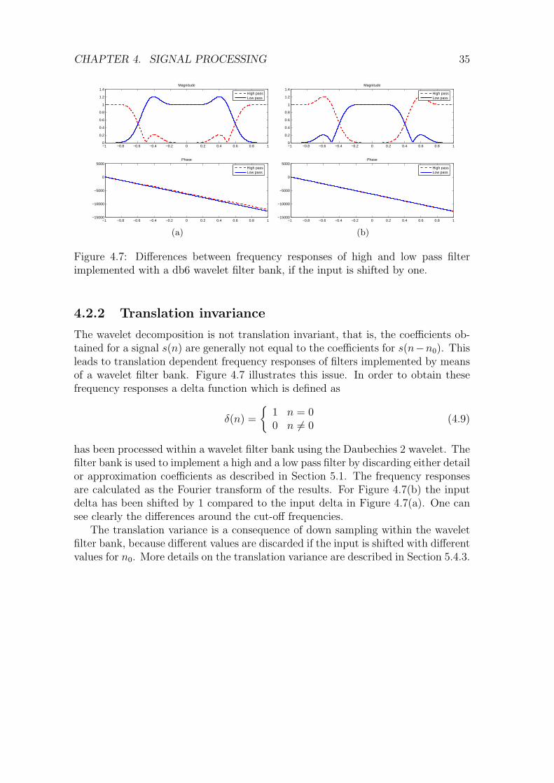
CHAPTER 4. SIGNAL PROCESSING 35
−1 −0.8 −0.6 −0.4 −0.2 0 0.2 0.4 0.6 0.8 10
0.2
0.4
0.6
0.8
1
1.2
1.4Magnitude
High passLow pass
−1 −0.8 −0.6 −0.4 −0.2 0 0.2 0.4 0.6 0.8 1−15000
−10000
−5000
0
5000Phase
High passLow pass
(a)
−1 −0.8 −0.6 −0.4 −0.2 0 0.2 0.4 0.6 0.8 10
0.2
0.4
0.6
0.8
1
1.2
1.4Magnitude
High passLow pass
−1 −0.8 −0.6 −0.4 −0.2 0 0.2 0.4 0.6 0.8 1−15000
−10000
−5000
0
5000Phase
High passLow pass
(b)
Figure 4.7: Differences between frequency responses of high and low pass filterimplemented with a db6 wavelet filter bank, if the input is shifted by one.
4.2.2 Translation invariance
The wavelet decomposition is not translation invariant, that is, the coefficients ob-tained for a signal s(n) are generally not equal to the coefficients for s(n−n0). Thisleads to translation dependent frequency responses of filters implemented by meansof a wavelet filter bank. Figure 4.7 illustrates this issue. In order to obtain thesefrequency responses a delta function which is defined as
δ(n) =
1 n = 00 n 6= 0
(4.9)
has been processed within a wavelet filter bank using the Daubechies 2 wavelet. Thefilter bank is used to implement a high and a low pass filter by discarding either detailor approximation coefficients as described in Section 5.1. The frequency responsesare calculated as the Fourier transform of the results. For Figure 4.7(b) the inputdelta has been shifted by 1 compared to the input delta in Figure 4.7(a). One cansee clearly the differences around the cut-off frequencies.
The translation variance is a consequence of down sampling within the waveletfilter bank, because different values are discarded if the input is shifted with differentvalues for n0. More details on the translation variance are described in Section 5.4.3.

CHAPTER 4. SIGNAL PROCESSING 36
4.3 Fast lifting wavelet transform
In this section a fast implementation of the wavelet transformation will be presented.Within this section FIR filters and signals are equivalently represented by their z-transforms. The z-transform of an FIR filter h(n) with M + 1 taps is defined as:
h(z) =M∑n=0
h(n)z−n. (4.10)
A convolution in time domain maps to a multiplication in z-domain [86], i.e. theconvolution h(n) ∗ x(n) can be written as h(z)x(z). The z-transforms of the FIRfilters are polynomials in z, also called Laurent polynomials. Having a polynomialrepresentation will appear to be a good notation to deduce the theory for the fastimplementation of a wavelet transformation.
In the classical implementation of the wavelet transformation two complemen-tary FIR filters h(z) and g(z) are applied to a signal s(z) and both results aresubsampled by a factor of 2 leading to a set of approximation coefficients aj and aset of detail coefficients dj. This implementation has the obvious drawback, thatevery second result value of the convolution with the FIR filter is discarded by thesubsampling. Consider the convolution with an FIR filter y(z) = h(z)x(z) followedby subsampling:
...
y0 = h0x0 + h1x−1z−1 + h2x−2z
−2 + . . .
y1 = h0x1 + h1x0z−1 + h2x−1z
−2 + . . .
y2 = h0x2 + h1x1z−1 + h2x0z
−2 + . . ....
Supposing that the odd rows are removed by the subsampling the remaining resultvalues in ye(z) are either obtained by
• even numbered filter coefficients he multiplied with even numbered samplesxe, or
• odd numbered filter coefficients ho mulitplied with odd numbered samples xo.
In other terms the FIR filter with subsequent downsampling (Figure 4.8) can berewritten as
ye(z) = he(z)xe(z) + z−1ho(z)xo(z) (4.11)
where he(z) and ho(z) are defined as
he(z) =∑n
h2nz−n and ho(z) =
∑n
h2n+1z−n. (4.12)
The delay z−1 in front of the odd part in (4.11) comes from the delay between evenand odd samples. Now we apply this remodeling of the FIR filter with subsequent
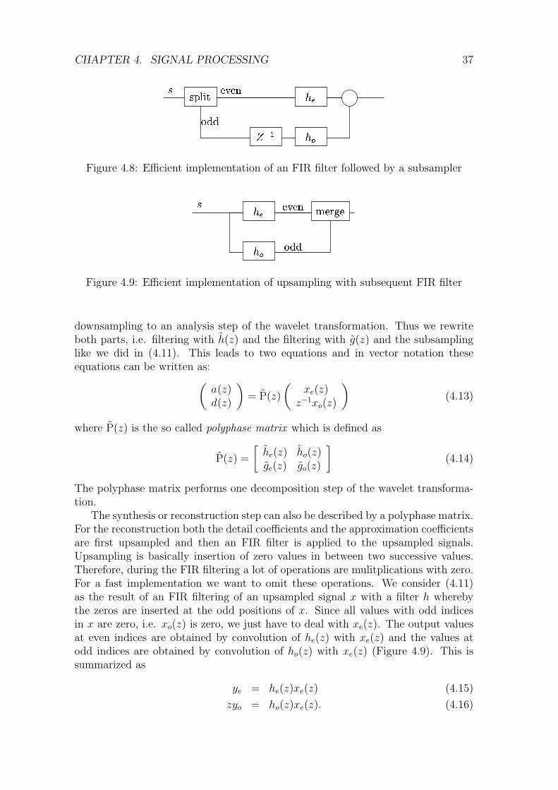
CHAPTER 4. SIGNAL PROCESSING 37
Figure 4.8: Efficient implementation of an FIR filter followed by a subsampler
Figure 4.9: Efficient implementation of upsampling with subsequent FIR filter
downsampling to an analysis step of the wavelet transformation. Thus we rewriteboth parts, i.e. filtering with h(z) and the filtering with g(z) and the subsamplinglike we did in (4.11). This leads to two equations and in vector notation theseequations can be written as:(
a(z)d(z)
)= P(z)
(xe(z)
z−1xo(z)
)(4.13)
where P(z) is the so called polyphase matrix which is defined as
P(z) =
[he(z) ho(z)ge(z) go(z)
](4.14)
The polyphase matrix performs one decomposition step of the wavelet transforma-tion.
The synthesis or reconstruction step can also be described by a polyphase matrix.For the reconstruction both the detail coefficients and the approximation coefficientsare first upsampled and then an FIR filter is applied to the upsampled signals.Upsampling is basically insertion of zero values in between two successive values.Therefore, during the FIR filtering a lot of operations are mulitplications with zero.For a fast implementation we want to omit these operations. We consider (4.11)as the result of an FIR filtering of an upsampled signal x with a filter h wherebythe zeros are inserted at the odd positions of x. Since all values with odd indicesin x are zero, i.e. xo(z) is zero, we just have to deal with xe(z). The output valuesat even indices are obtained by convolution of he(z) with xe(z) and the values atodd indices are obtained by convolution of ho(z) with xe(z) (Figure 4.9). This issummarized as
ye = he(z)xe(z) (4.15)
zyo = ho(z)xe(z). (4.16)
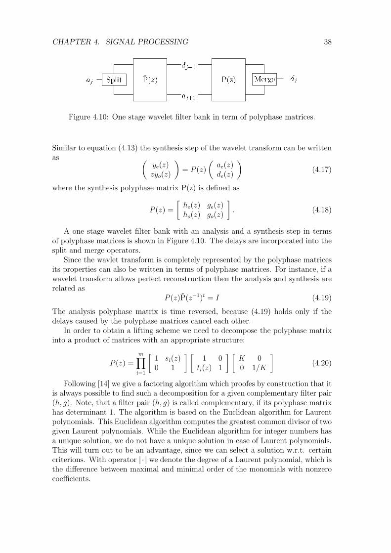
CHAPTER 4. SIGNAL PROCESSING 38
! "# $
Figure 4.10: One stage wavelet filter bank in term of polyphase matrices.
Similar to equation (4.13) the synthesis step of the wavelet transform can be writtenas (
ye(z)zyo(z)
)= P (z)
(ae(z)de(z)
)(4.17)
where the synthesis polyphase matrix P(z) is defined as
P (z) =
[he(z) ge(z)ho(z) go(z)
]. (4.18)
A one stage wavelet filter bank with an analysis and a synthesis step in termsof polyphase matrices is shown in Figure 4.10. The delays are incorporated into thesplit and merge operators.
Since the wavlet transform is completely represented by the polyphase matricesits properties can also be written in terms of polyphase matrices. For instance, if awavelet transform allows perfect reconstruction then the analysis and synthesis arerelated as
P (z)P(z−1)t = I (4.19)
The analysis polyphase matrix is time reversed, because (4.19) holds only if thedelays caused by the polyphase matrices cancel each other.
In order to obtain a lifting scheme we need to decompose the polyphase matrixinto a product of matrices with an appropriate structure:
P (z) =m∏i=1
[1 si(z)0 1
] [1 0
ti(z) 1
] [K 00 1/K
](4.20)
Following [14] we give a factoring algorithm which proofes by construction that itis always possible to find such a decomposition for a given complementary filter pair(h, g). Note, that a filter pair (h, g) is called complementary, if its polyphase matrixhas determinant 1. The algorithm is based on the Euclidean algorithm for Laurentpolynomials. This Euclidean algorithm computes the greatest common divisor of twogiven Laurent polynomials. While the Euclidean algorithm for integer numbers hasa unique solution, we do not have a unique solution in case of Laurent polynomials.This will turn out to be an advantage, since we can select a solution w.r.t. certaincriterions. With operator | · | we denote the degree of a Laurent polynomial, which isthe difference between maximal and minimal order of the monomials with nonzerocoefficients.

CHAPTER 4. SIGNAL PROCESSING 39
Euclidean Algorithm for Laurent polynomials as given in [14]
Take two Laurent polynomials a(z) and b(z) 6= 0 with |a(z)| ≥|b(z)|. Let a0(z) := a(z) and b0(z) := b(z) and iterate the followingsteps starting from i = 0 until bi(z) = 0:
1. Choose bi+1(z) and qi+1(z) such that
|bi+1(z)| < |bi(z)| and
ai(z) = bi(z)qi+1(z) + bi+1(z)
2. Let ai+1(z) := bi(z)
3. Increment i.
Then an(z) = gcd(a(z), b(z)) where n is the smallest number forwhich bn(z) = 0.
At each step we must make sure that |bi+1(z)| < |bi(z)|. Then there is an mat which |bm(z)| = 0 and the algorithm finishes after n = m + 1 steps. Thereforethe number of steps is bound by n ≤ |b(z)| + 1. However, this is the number ofsteps to find a single solution. At each step we can decide which monomials shouldbe eliminated by the division. This means that there are different possibilities forbi+1(z). For example, if |ai(z)| = 3 and |bi(z)| = 2 there are three solutions forbi+1(z). We will use an example which is also given in [14] to clearify this. Leta(z) = z−1 + 6 + z and b(z) = 4 + 4z. Now find a polynomial q(z) of degree 1 sothat the remainder r(z) given as
r(z) = a(z)− b(z)q(z) (4.21)
has degree zero, i.e. degree of b(z) minus 1. There are three solutions:
r(z) = (z−1 + 6 + z)− (4 + 4z) (1
4z−1 +
5
4) = −4z
r(z) = (z−1 + 6 + z)− (4 + 4z) (1
4z−1 +
1
4) = 4
r(z) = (z−1 + 6 + z)− (4 + 4z) (5
4z−1 +
1
4) = −4z−1
In the first solution we have eliminated the term in z−1 and the constant, in thesecond solution the terms in z−1 and in z, and finally in the third solution theconstant and the term in z. Either of these r(z) is a possible value for bi+1(z), givenbi(z) = b(z) and ai(z) = a(z).
A particular filter pair (h, g) is factorized into lifting steps by applying the Eu-clidean algorithm with a0(z) = he(z) and b0(z) = ho(z). Note, that we can alwaysfind a constant greatest common divisor K as we start with a complementary filterpair (h, g) which polyphase matrix has determinant 1 by definition. This implies thatthe Laurent polynomials he(z) and ho(z) are relative prime, because any common
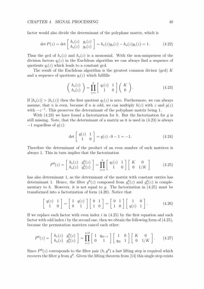
CHAPTER 4. SIGNAL PROCESSING 40
factor would also divide the determinant of the polyphase matrix, which is
detP (z) = det
[he(z) ge(z)ho(z) go(z)
]= he(z)go(z)− ho(z)ge(z) = 1. (4.22)
Thus the gcd of he(z) and ho(z) is a monomial. With the non-uniqueness of thedivision factors qi(z) in the Euclidean algorithm we can always find a sequence ofquotients qi(z) which leads to a constant gcd.
The result of the Euclidean algorithm is the greatest common divisor (gcd) Kand a sequence of quotients qi(z) which fullfills(
he(z)ho(z)
)=
n∏i=1
[qi(z) 1
1 0
](K0
). (4.23)
If |ho(z)| > |he(z)| then the first quotient q1(z) is zero. Furthermore, we can alwaysassume, that n is even, because if n is odd, we can multiply h(z) with z and g(z)with −z−1. This preserves the determinant of the polyphase matrix being 1.
With (4.23) we have found a factorization for h. But the factorization for g isstill missing. Note, that the determinant of a matrix as it is used in (4.23) is always−1 regardless of q(z):
det
[q(z) 1
1 0
]= q(z) · 0− 1 = −1. (4.24)
Therefore the determinant of the product of an even number of such matrices isalways 1. This in turn implies that the factorization
P 0(z) =
[he(z) g0
e(z)ho(z) g0
o(z)
]=
n∏i=1
[qi(z) 1
1 0
] [K 00 1/K
](4.25)
has also determinant 1, as the determinant of the matrix with constant entries hasdeterminant 1. Hence, the filter g0(z) composed from g0
e(z) and g0o(z) is comple-
mentary to h. However, it is not equal to g. The factorization in (4.25) must betransformed into a factorization of form (4.20). Notice that[
q(z) 11 0
]=
[1 q(z)0 1
] [0 11 0
]=
[0 11 0
] [1 0q(z) 1
]. (4.26)
If we replace each factor with even index i in (4.25) by the first equation and eachfactor with odd index i by the second one, then we obtain the following form of (4.25),because the permutation matrices cancel each other:
P 0(z) =
[he(z) g0
e(z)ho(z) g0
o(z)
]=
n/2∏i=1
[1 q2i−1
0 1
] [1 0q2i 1
] [K 00 1/K
]. (4.27)
Since P 0(z) corresponds to the filter pair (h, g0) a last lifting step is required whichrecovers the filter g from g0. Given the lifting theorem from [14] this single step exists
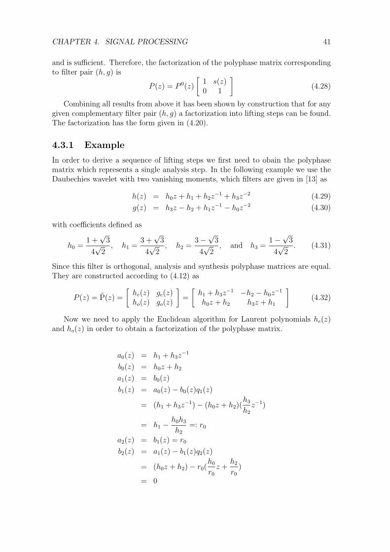
CHAPTER 4. SIGNAL PROCESSING 41
and is sufficient. Therefore, the factorization of the polyphase matrix correspondingto filter pair (h, g) is
P (z) = P 0(z)
[1 s(z)0 1
](4.28)
Combining all results from above it has been shown by construction that for anygiven complementary filter pair (h, g) a factorization into lifting steps can be found.The factorization has the form given in (4.20).
4.3.1 Example
In order to derive a sequence of lifting steps we first need to obain the polyphasematrix which represents a single analysis step. In the following example we use theDaubechies wavelet with two vanishing moments, which filters are given in [13] as
h(z) = h0z + h1 + h2z−1 + h3z
−2 (4.29)
g(z) = h3z − h2 + h1z−1 − h0z
−2 (4.30)
with coefficients defined as
h0 =1 +√
3
4√
2, h1 =
3 +√
3
4√
2, h2 =
3−√
3
4√
2, and h3 =
1−√
3
4√
2. (4.31)
Since this filter is orthogonal, analysis and synthesis polyphase matrices are equal.They are constructed according to (4.12) as
P (z) = P(z) =
[he(z) ge(z)ho(z) go(z)
]=
[h1 + h3z
−1 −h2 − h0z−1
h0z + h2 h3z + h1
](4.32)
Now we need to apply the Euclidean algorithm for Laurent polynomials he(z)and ho(z) in order to obtain a factorization of the polyphase matrix.
a0(z) = h1 + h3z−1
b0(z) = h0z + h2
a1(z) = b0(z)
b1(z) = a0(z)− b0(z)q1(z)
= (h1 + h3z−1)− (h0z + h2)(
h3
h2
z−1)
= h1 −h0h3
h2
=: r0
a2(z) = b1(z) = r0
b2(z) = a1(z)− b1(z)q2(z)
= (h0z + h2)− r0(h0
r0
z +h2
r0
)
= 0
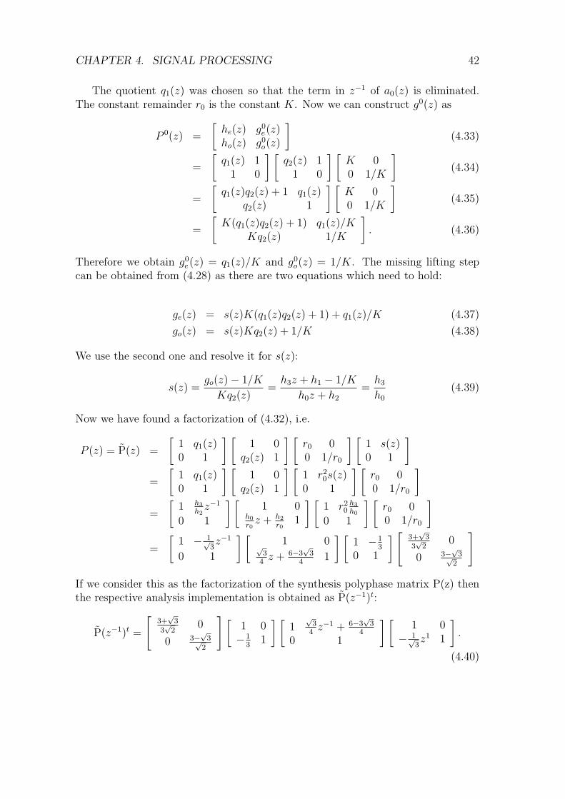
CHAPTER 4. SIGNAL PROCESSING 42
The quotient q1(z) was chosen so that the term in z−1 of a0(z) is eliminated.The constant remainder r0 is the constant K. Now we can construct g0(z) as
P 0(z) =
[he(z) g0
e(z)ho(z) g0
o(z)
](4.33)
=
[q1(z) 1
1 0
] [q2(z) 1
1 0
] [K 00 1/K
](4.34)
=
[q1(z)q2(z) + 1 q1(z)
q2(z) 1
] [K 00 1/K
](4.35)
=
[K(q1(z)q2(z) + 1) q1(z)/K
Kq2(z) 1/K
]. (4.36)
Therefore we obtain g0e(z) = q1(z)/K and g0
o(z) = 1/K. The missing lifting stepcan be obtained from (4.28) as there are two equations which need to hold:
ge(z) = s(z)K(q1(z)q2(z) + 1) + q1(z)/K (4.37)
go(z) = s(z)Kq2(z) + 1/K (4.38)
We use the second one and resolve it for s(z):
s(z) =go(z)− 1/K
Kq2(z)=h3z + h1 − 1/K
h0z + h2
=h3
h0
(4.39)
Now we have found a factorization of (4.32), i.e.
P (z) = P(z) =
[1 q1(z)0 1
] [1 0
q2(z) 1
] [r0 00 1/r0
] [1 s(z)0 1
]=
[1 q1(z)0 1
] [1 0
q2(z) 1
] [1 r2
0s(z)0 1
] [r0 00 1/r0
]=
[1 h3
h2z−1
0 1
] [1 0
h0
r0z + h2
r01
] [1 r2
0h3
h0
0 1
] [r0 00 1/r0
]=
[1 − 1√
3z−1
0 1
] [1 0√
34z + 6−3
√3
41
] [1 −1
3
0 1
][ 3+√
33√
20
0 3−√
3√2
]
If we consider this as the factorization of the synthesis polyphase matrix P(z) thenthe respective analysis implementation is obtained as P(z−1)t:
P(z−1)t =
[3+√
33√
20
0 3−√
3√2
] [1 0−1
31
] [1
√3
4z−1 + 6−3
√3
4
0 1
] [1 0
− 1√3z1 1
].
(4.40)

CHAPTER 4. SIGNAL PROCESSING 43
The steps of the implementation are derived from this factorization as:
d(0)l = x[2l + 1] (4.41)
a(0)l = x[2l] (4.42)
d(1)l = d
(0)l − 1/
√3a
(0)l+1 (4.43)
a(1)l = a
(0)l + (6− 3
√3)/4d
(1)l +
√3/4d
(1)l−1 (4.44)
d(2)l = d
(1)l − 1/3a
(1)l (4.45)
a(2)l = (3 +
√3)/(3
√2)a
(1)l (4.46)
d(3)l = (3−
√3)/(√
2)d(2)l (4.47)
(4.48)
The inverse, i.e. the synthesis step can be easily derived by reversing the orderand changing the signs of the previous steps.
4.3.2 Mapping onto integer values
The lifting scheme can be modified such that it maps integers onto integers, whilecomputing the coefficients in floating point arithmetic. We introduce a roundingfunction each time we need to update the coefficients dj or aj. However, the iterationusually includes a scaling as last step which is not invertible without loss if the resultis rounded. But we can replace the two scaling steps by four lifting steps, wherebythe first lifiting step of the scaling can always be merged with the last lifting step ofthe factorization [14]. Scaling has the following different factorizations:
P (z) =
[K 00 1/K
]=
[1 K −K2
0 1
] [1 0
−1/K 1
] [1 K − 10 1
] [1 01 1
](4.49)
or
P (z) =
[K 00 1/K
]=
[1 0−1 1
] [1 1− 1/K0 1
] [1 0K 1
] [1 1/K2 − 1/K0 1
]. (4.50)
We apply (4.49) to (4.41) and add the rounding. This leads to the following im-plementation, which maps integer values onto integer values, whereby K = (3 +√
3)/(3√
2) and [·] denotes the rounding operation.
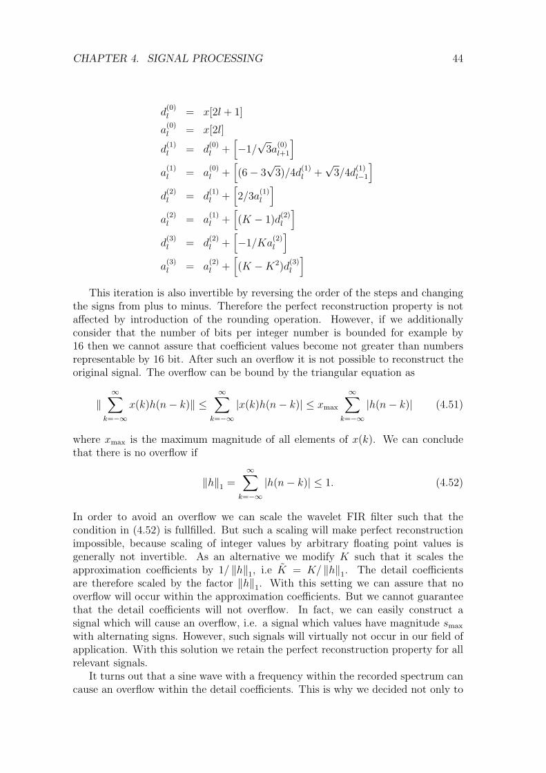
CHAPTER 4. SIGNAL PROCESSING 44
d(0)l = x[2l + 1]
a(0)l = x[2l]
d(1)l = d
(0)l +
[−1/√
3a(0)l+1
]a
(1)l = a
(0)l +
[(6− 3
√3)/4d
(1)l +
√3/4d
(1)l−1
]d
(2)l = d
(1)l +
[2/3a
(1)l
]a
(2)l = a
(1)l +
[(K − 1)d
(2)l
]d
(3)l = d
(2)l +
[−1/Ka
(2)l
]a
(3)l = a
(2)l +
[(K −K2)d
(3)l
]This iteration is also invertible by reversing the order of the steps and changing
the signs from plus to minus. Therefore the perfect reconstruction property is notaffected by introduction of the rounding operation. However, if we additionallyconsider that the number of bits per integer number is bounded for example by16 then we cannot assure that coefficient values become not greater than numbersrepresentable by 16 bit. After such an overflow it is not possible to reconstruct theoriginal signal. The overflow can be bound by the triangular equation as
‖∞∑
k=−∞
x(k)h(n− k)‖ ≤∞∑
k=−∞
|x(k)h(n− k)| ≤ xmax
∞∑k=−∞
|h(n− k)| (4.51)
where xmax is the maximum magnitude of all elements of x(k). We can concludethat there is no overflow if
‖h‖1 =∞∑
k=−∞
|h(n− k)| ≤ 1. (4.52)
In order to avoid an overflow we can scale the wavelet FIR filter such that thecondition in (4.52) is fullfilled. But such a scaling will make perfect reconstructionimpossible, because scaling of integer values by arbitrary floating point values isgenerally not invertible. As an alternative we modify K such that it scales theapproximation coefficients by 1/ ‖h‖1, i.e K = K/ ‖h‖1. The detail coefficientsare therefore scaled by the factor ‖h‖1. With this setting we can assure that nooverflow will occur within the approximation coefficients. But we cannot guaranteethat the detail coefficients will not overflow. In fact, we can easily construct asignal which will cause an overflow, i.e. a signal which values have magnitude smax
with alternating signs. However, such signals will virtually not occur in our field ofapplication. With this solution we retain the perfect reconstruction property for allrelevant signals.
It turns out that a sine wave with a frequency within the recorded spectrum cancause an overflow within the detail coefficients. This is why we decided not only to

CHAPTER 4. SIGNAL PROCESSING 45
provide an integer based wavelet filter bank but also a floating point version. Thisversion was implemented on the host side and utilizes the Pentium instruction setextensions for signal processing.
The main drawback of mapping to integer coefficients are quantization errors.The rounding operation modifies the contents of the different frequency bands. Ifthe coefficients are not changed then this effect cancels out during reconstruction.So integer coefficients are e.g. suitable for lossless compression. However, if weimplement a filter based on modifications of the coefficients, then the reconstructedsignal suffers from quantization errors. The strategy described above which is sup-posed to avoid overflows increases the quantization errors even more. Also the effectof translation variance becomes larger.
As a consequence the mapping on integer coefficients is not optimal for ourapplication..
4.3.3 Implementing lifting steps on a C6701
The actual implementation of the lifting scheme on a DSP includes serveral steps.In this section will give an overview on how to create an optimized assembly routinegiven a factorization of a polyphase matrix.
We will implement the Daubechies wavelet with three vanishing moments whichcan be factorized as follows:
[K 00 1/K
] [1 λ0 1
] [1 0
εz−1 1
] [1 δ0 1
] [1 0γ 1
] [1 βz + β′
0 1
] [1 0α 1
](4.53)
where
α = +4.122865950520000e− 01
β = +1.565136279631000e+ 00
β′ = +4.160137790400000e− 02
γ = −2.814352831900000e− 02
δ = −3.984066649260000e− 01
ε = −4.812981574140000e− 01
λ = +3.984066649266020e− 01
K = +5.155407358530000e− 01
We used a tool which computes all possible factorizations given a pair of comple-mentary FIR filters. From this set of factorizations one was choosen w.r.t. a numberof criterions:
• Number of lifting steps should be high
• Each lifting step should have at most order 1, i.e. only previous or next valuefrom previous step is used
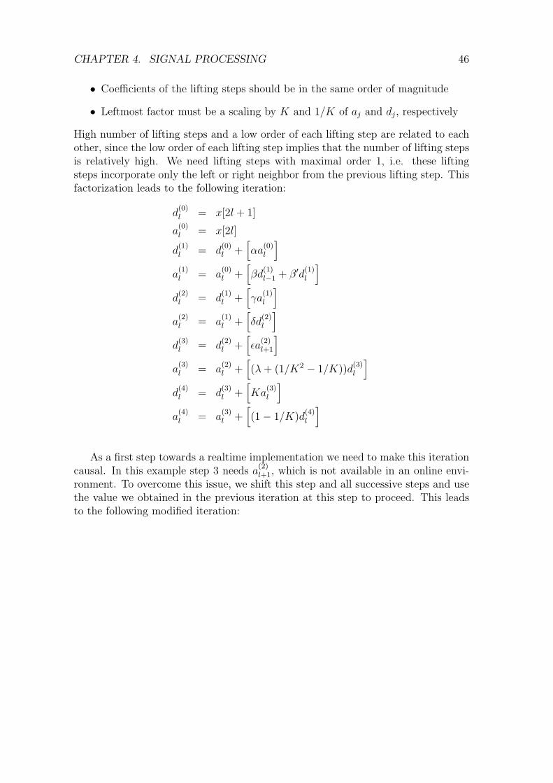
CHAPTER 4. SIGNAL PROCESSING 46
• Coefficients of the lifting steps should be in the same order of magnitude
• Leftmost factor must be a scaling by K and 1/K of aj and dj, respectively
High number of lifting steps and a low order of each lifting step are related to eachother, since the low order of each lifting step implies that the number of lifting stepsis relatively high. We need lifting steps with maximal order 1, i.e. these liftingsteps incorporate only the left or right neighbor from the previous lifting step. Thisfactorization leads to the following iteration:
d(0)l = x[2l + 1]
a(0)l = x[2l]
d(1)l = d
(0)l +
[αa
(0)l
]a
(1)l = a
(0)l +
[βd
(1)l−1 + β′d
(1)l
]d
(2)l = d
(1)l +
[γa
(1)l
]a
(2)l = a
(1)l +
[δd
(2)l
]d
(3)l = d
(2)l +
[εa
(2)l+1
]a
(3)l = a
(2)l +
[(λ+ (1/K2 − 1/K))d
(3)l
]d
(4)l = d
(3)l +
[Ka
(3)l
]a
(4)l = a
(3)l +
[(1− 1/K)d
(4)l
]
As a first step towards a realtime implementation we need to make this iterationcausal. In this example step 3 needs a
(2)l+1, which is not available in an online envi-
ronment. To overcome this issue, we shift this step and all successive steps and usethe value we obtained in the previous iteration at this step to proceed. This leadsto the following modified iteration:

CHAPTER 4. SIGNAL PROCESSING 47
d(0)l = x[2l + 1]
a(0)l = x[2l]
d(1)l = d
(0)l +
[αa
(0)l
]a
(1)l = a
(0)l +
[βd
(1)l−1 + β′d
(1)l
]d
(2)l = d
(1)l +
[γa
(1)l
]a
(2)l = a
(1)l +
[δd
(2)l
]d
(3)l−1 = d
(2)l−1 +
[εa
(2)l
]a
(3)l−1 = a
(2)l−1 +
[(λ+ (1/K2 − 1/K))d
(3)l−1
]d
(4)l−1 = d
(3)l−1 +
[Ka
(3)l−1
]a
(4)l−1 = a
(3)l−1 +
[(1− 1/K)d
(4)l−1
]
From this iteration we derived that we need to keep track on three states ineach iteration, i.e. d
(1)l−1, d
(2)l−1, and a
(2)l−1 which are all not available from the current
iteration. In the implementation we deal with three main data structures: the signalx, the constants denoted by c, and the states denoted by s. Constants and statesare stored in arrays of 32 bit elements with predetermined length – known e.g. atcompile time. The constants are always float values and we will assume that thestates are always 32 bit integer numbers. All equations basically have the samestructure and can be implemented by similar sequences of assembler instructions.This is illustrated for a single equation:
a(1)l = a
(0)l +
[βd
(1)l−1 + β′d
(1)l
](4.54)
LDW c[β], cst load constant β
LDW s[d(1)l−1], temp1 load d
(1)l−1 from s
STW d, s[d(1)l−1] update d
(1)l−1 in s with d
(1)l
INTSP temp1, temp1 convert d(1)l−1 to single precision
MPYSP cst, temp1, temp1 multiply constant β and d(1)l−1
INTSP d, temp0 convert d(1)l to single precision
LDW c[β′], cst load constant β′
MPYSP cst, temp0, temp1, temp0 multiply constant β′ and d(1)l
ADDSP temp0, temp1, temp0 add results of previous productsSPINT temp0 convert it to integer
ADD temp0, a, a add this to a(0)l and obtain a
(1)l

CHAPTER 4. SIGNAL PROCESSING 48
Figure 4.11: Organization of wavelet coefficients during the decomposition with thelifting algorithm. A block of 8 coefficient is completely decomposed, i.e. in threedecomposition steps. The last row shows that the coefficients of the different levelsare interleaved according to the so called lifting order.
This sequence of assembler commands is not well suited for optimization usingthe capabilities of the C6701. Mostly results from an assembly instruction areneeded for the next instruction. This prevents us from using pipelining and parallelinstructions for direct acceleration of the iteration. On the other hand, we canprocess multiple signals in parallel. In fact, the iteration uses only a small numberof registers for a single signal. Moreover, some of these registers can be reused forall signals, as the constants pointer, the constant value (cst), and the states pointer.Futhermore we can assume that the sample values of the signals are particularlyarranged in memory so that we can efficiently retrieve samples from multiple signals.Four registers, i.e. a, d, temp0, and temp1 are needed individually for each signal.
We developed a semiautomatic tool which can generate linear assembler routinesthat implement wavelet decomposition and reconstruction algorithm based on thelifting scheme.
The generated code uses the capabilities of the C6701 at a great extend. Thebasic optimization strategy was to process multiple channels in parallel. Note, that’in parallel’ is meant literally. The C6701 has two register sets, each having 16 gen-eral purpose registers of 32 bit width. Each register set is associated with severaloperation units, which can perform operations in parallel. We managed to processfour channels in parallel. This implementation uses the minimum number of regis-ters per channel. However, all the 32 registers are directly or indirectly (counters,parameters) neccessary for the optimized implementation.
In Figure 4.12 a fragment of the generated assembler code is shown. These

CHAPTER 4. SIGNAL PROCESSING 49
; Step 1, predict
|| LDW .D2T2 *+c[1],cst2 ; load constant
LDDW .D1T1 *+states1[0],temp1_i:temp1_ii ;
|| LDDW .D2T2 *+states2[1],temp1_iii:temp1_iv ;
STW .D1T1 a_i,*+states1[0] ;
|| STW .D2T2 a_iii,*+states2[2] ;
STW .D1T1 a_ii,*+states1[1] ;
|| STW .D2T2 a_iv,*+states2[3] ;
ADDAW .D1 states1,4,states1 ;
|| ADDAW .D2 states2,4,states2 ;
MPYSP .M1 temp1_i,cst2,temp1_i ;
|| MPYSP .M2 temp1_iii,cst2,temp1_iii ;
MPYSP .M1 temp1_ii,cst2,temp1_ii ;
|| MPYSP .M2 temp1_iv,cst2,temp1_iv ;
|| LDW .D2T2 *+c[2],cst2 ; load constant
MV .L1 a_i,temp2_i ;
|| MV .D1 a_ii,temp2_ii ;
|| MV .L2 a_iii,temp2_iii ;
|| MV .D2 a_iv,temp2_iv ;
MPYSP .M1 temp2_i,cst2,temp2_i ;
|| MPYSP .M2 temp2_iii,cst2,temp2_iii ;
MPYSP .M1 temp2_ii,cst2,temp2_ii ;
|| MPYSP .M2 temp2_iv,cst2,temp2_iv ;
ADDSP .L1 temp1_i,temp2_i,temp1_i ;
|| ADDSP .L2 temp1_iii,temp2_iii,temp1_iii ;
ADDSP .L1 temp1_ii,temp2_ii,temp1_ii ;
|| ADDSP .L2 temp1_iv,temp2_iv,temp1_iv ;
LDDW .D1T1 *+states1[2],temp2_i:temp2_ii ;
|| LDDW .D2T2 *+states2[3],temp2_iii:temp2_iv ;
LDDW .D1T1 *+states1[0],temp3_i:temp3_ii ;
|| LDDW .D2T2 *+states2[1],temp3_iii:temp3_iv ;
STW .D1T1 temp2_i,*+states1[0];
|| STW .D2T2 temp2_iii,*+states2[2];
STW .D1T1 temp2_ii,*+states1[1];
|| STW .D2T2 temp2_iv,*+states2[3];
STW .D1T1 d_i,*+states1[4] ;
|| STW .D2T2 d_iii,*+states2[6] ;
STW .D1T1 d_ii,*+states1[5] ;
|| STW .D2T2 d_iv,*+states2[7] ;
ADDAW .D1 states1,8,states1 ;
|| ADDAW .D2 states2,8,states2 ;
SPINT .L1 temp3_i,temp3_i ;
|| SPINT .L2 temp3_iii,temp3_iii ;
SPINT .L1 temp3_ii,temp3_ii ;
|| SPINT .L2 temp3_iv,temp3_iv ;
SPINT .L1 temp1_i,temp1_i ;
|| SPINT .L2 temp1_iii,temp1_iii ;
SPINT .L1 temp1_ii,temp1_ii ;
|| SPINT .L2 temp1_iv,temp1_iv ;
ADD .S1 temp3_i,temp1_i,d_i ;
|| ADD .D1 temp3_ii,temp1_ii,d_ii ;
|| ADD .S2 temp3_iii,temp1_iii,d_iii ;
|| ADD .D2 temp3_iv,temp1_iv,d_iv ;
INTSP .L1 d_i,d_i ;
|| INTSP .L2 d_iii,d_iii ;
INTSP .L1 d_ii,d_ii ;
|| INTSP .L2 d_iv,d_iv ;
Figure 4.12: Linear assembler code fragment which implements a prediction liftingstep.
instructions implement a prediction lifting step like
d(k+1)l = d
(k)l +
[c0a
(k)l−1 + c1a
(k)l−2
](4.55)
where the brackets denote the rounding operation. An assembly code line has fourcolumns: optional parallel bars, instruction, operation unit, operands. The parallelbars || indicate parallel execution of the instructions in this line and the previousline. Execution of one instruction happens in serveral phases, where its number dif-fers from instruction to instruction. The MV instruction only needs one phase, whilethe LDW needs five phases. Therefore the constants loaded from c[1] is availablein cst2 at the fifth parallel bar. Note, that the linear assembler is translated intothe actual assembler, and during translation NOPs are inserted where needed. Oneway to optimize the code is to rearrange the instructions such that as few NOPs aspossible are inserted. Because we process four channels in parallel we can make anefficient use of as many operation units as possible.
The equivalent C code which processed a single channel is
/* Step 1, predict */
cst = c[1];
temp1 = states[1];
states[1] = a;
temp1 = temp1 * cst;
cst = c[2];
temp2 = a;
temp2 = temp2 * cst;
temp1 = temp1 + temp2;
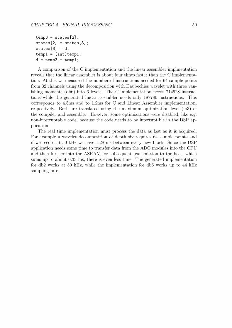
CHAPTER 4. SIGNAL PROCESSING 50
temp3 = states[2];
states[2] = states[3];
states[3] = d;
temp1 = (int)temp1;
d = temp3 + temp1;
A comparison of the C implementation and the linear assembler implmentationreveals that the linear assembler is about four times faster than the C implementa-tion. At this we measured the number of instructions needed for 64 sample pointsfrom 32 channels using the decomposition with Daubechies wavelet with three van-ishing moments (db6) into 6 levels. The C implementation needs 714928 instruc-tions while the generated linear assembler needs only 187780 instructions. Thiscorresponds to 4.5ms and to 1.2ms for C and Linear Assembler implementation,respectively. Both are translated using the maximum optimization level (-o3) ofthe compiler and assembler. However, some optimizations were disabled, like e.g.non-interruptable code, because the code needs to be interruptible in the DSP ap-plication.
The real time implementation must process the data as fast as it is acquired.For example a wavelet decomposition of depth six requires 64 sample points andif we record at 50 kHz we have 1.28 ms between every new block. Since the DSPapplication needs some time to transfer data from the ADC modules into the CPUand then further into the ASRAM for subsequent transmission to the host, whichsums up to about 0.33 ms, there is even less time. The generated implementationfor db2 works at 50 kHz, while the implementation for db6 works up to 44 kHzsampling rate.
Chapter 5
Applying Wavelet Transform toNeural Signals
5.1 Low pass, band pass, and high pass wavelet
filter
A wavelet filter bank can be used to implement low pass, band pass, and high passfilter. This is simply done by setting the coefficients to zero, which represent thefrequency band, that should be suppressed. For instance setting the coefficientsaL−1 to zero yields a high pass filter, and elimination of the coefficients d0 a lowpass filter. One drawback of this method is that we cannot choose the cut offfrequencies for the high pass, band pass, or low pass filters arbitrarily. Insteadwe are restricted to positions that are presentable as sampling rate divided by 2j
(j ∈ N, j > 0). However, this restriction does not pose a problem for applications inneural recordings. In Figure 5.1 an example of a high pass filtered signal is shown.The lower trace is the original neural recording acquired at 5 kHz, while the uppertrace is the result of high pass filtering using a Daubechies 2 wavelet filter bank ofdepth 4. The approximation coefficients which correspond to the frequency bandfrom DC up to 312.5 Hz (= 5.000 Hz/24) are set to zero before reconstruction. Thisimplements a high pass filter with cut-off frequency at 312.5 Hz. Note, that thisfilter nicely preserves the shape of the action potentials, as the wavelet filter bankbased high pass has a nearly linear phase (see also Section 4.2.1).
5.2 Compression and Denoising
Denoising and compression are related due to the fact that denoising techniquescan be used to implement lossy compression [11], or in other words we can use alossy compression scheme which denoises the signal. To grasp the idea behind that,consider that a typical signal like e.g. a neural recording usually contains some struc-tural correlation which in turn is exploited by a good compression scheme. But aneural recording does also contain noise. As noise, in particular white noise, does nothave any structural redundancies, it is difficult to compress it effectively. However,denoising the signal, yields a signal which can be compressed more effectively.
51
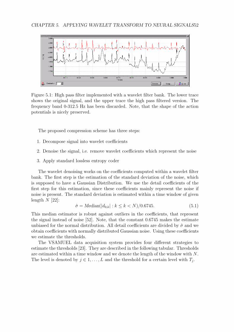
CHAPTER 5. APPLYING WAVELET TRANSFORM TO NEURAL SIGNALS52
Figure 5.1: High pass filter implemented with a wavelet filter bank. The lower traceshows the original signal, and the upper trace the high pass filtered version. Thefrequency band 0-312.5 Hz has been discarded. Note, that the shape of the actionpotentials is nicely preserved.
The proposed compression scheme has three steps:
1. Decompose signal into wavelet coefficients
2. Denoise the signal, i.e. remove wavelet coefficients which represent the noise
3. Apply standard lossless entropy coder
The wavelet denoising works on the coefficients computed within a wavelet filterbank. The first step is the estimation of the standard deviation of the noise, whichis supposed to have a Gaussian Distribution. We use the detail coefficients of thefirst step for this estimation, since these coefficients mainly represent the noise ifnoise is present. The standard deviation is estimated within a time window of givenlength N [22]:
σ = Median(|d0,k| : k ≤ k < N)/0.6745. (5.1)
This median estimator is robust against outliers in the coefficients, that representthe signal instead of noise [52]. Note, that the constant 0.6745 makes the estimateunbiased for the normal distribution. All detail coefficients are divided by σ and weobtain coefficients with normally distributed Gaussian noise. Using these coefficientswe estimate the thresholds.
The VSAMUEL data acquisition system provides four different strategies toestimate the thresholds [23]. They are described in the following tabular. Thresholdsare estimated within a time window and we denote the length of the window with N .The level is denoted by j ∈ 1, . . . , L and the threshold for a certain level with Tj.
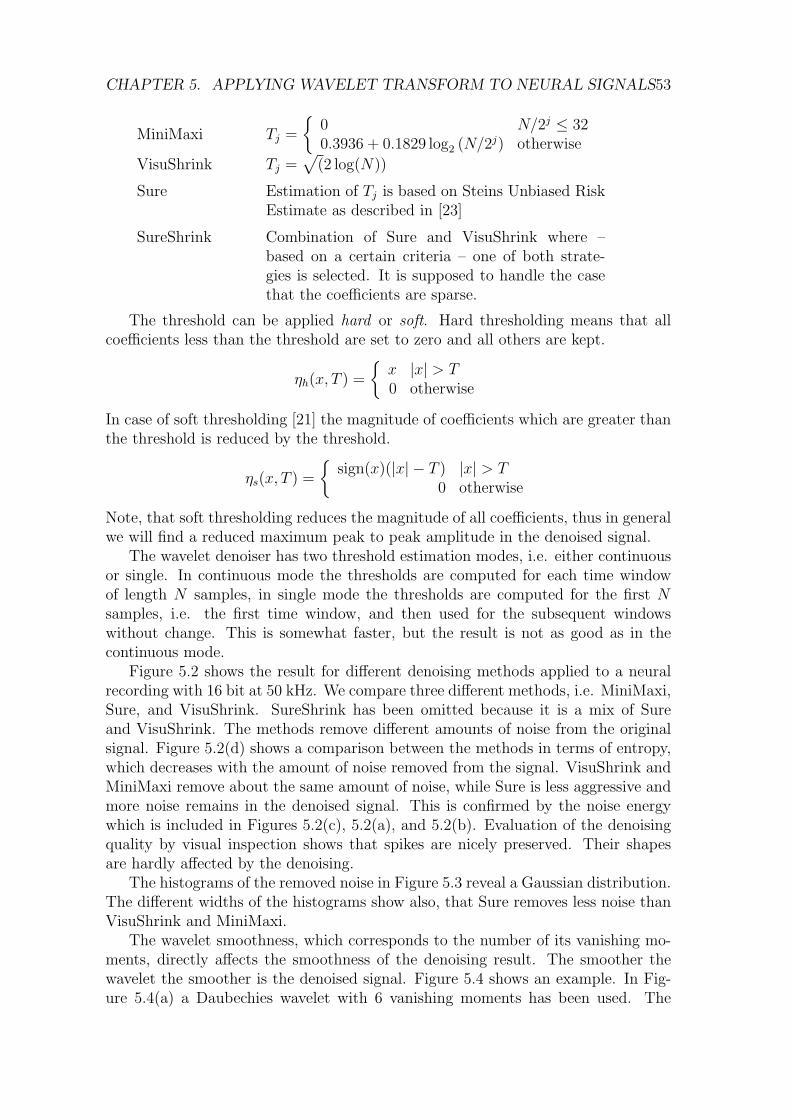
CHAPTER 5. APPLYING WAVELET TRANSFORM TO NEURAL SIGNALS53
MiniMaxi Tj =
0 N/2j ≤ 320.3936 + 0.1829 log2 (N/2j) otherwise
VisuShrink Tj =√
(2 log(N))
Sure Estimation of Tj is based on Steins Unbiased RiskEstimate as described in [23]
SureShrink Combination of Sure and VisuShrink where –based on a certain criteria – one of both strate-gies is selected. It is supposed to handle the casethat the coefficients are sparse.
The threshold can be applied hard or soft. Hard thresholding means that allcoefficients less than the threshold are set to zero and all others are kept.
ηh(x, T ) =
x |x| > T0 otherwise
In case of soft thresholding [21] the magnitude of coefficients which are greater thanthe threshold is reduced by the threshold.
ηs(x, T ) =
sign(x)(|x| − T ) |x| > T
0 otherwise
Note, that soft thresholding reduces the magnitude of all coefficients, thus in generalwe will find a reduced maximum peak to peak amplitude in the denoised signal.
The wavelet denoiser has two threshold estimation modes, i.e. either continuousor single. In continuous mode the thresholds are computed for each time windowof length N samples, in single mode the thresholds are computed for the first Nsamples, i.e. the first time window, and then used for the subsequent windowswithout change. This is somewhat faster, but the result is not as good as in thecontinuous mode.
Figure 5.2 shows the result for different denoising methods applied to a neuralrecording with 16 bit at 50 kHz. We compare three different methods, i.e. MiniMaxi,Sure, and VisuShrink. SureShrink has been omitted because it is a mix of Sureand VisuShrink. The methods remove different amounts of noise from the originalsignal. Figure 5.2(d) shows a comparison between the methods in terms of entropy,which decreases with the amount of noise removed from the signal. VisuShrink andMiniMaxi remove about the same amount of noise, while Sure is less aggressive andmore noise remains in the denoised signal. This is confirmed by the noise energywhich is included in Figures 5.2(c), 5.2(a), and 5.2(b). Evaluation of the denoisingquality by visual inspection shows that spikes are nicely preserved. Their shapesare hardly affected by the denoising.
The histograms of the removed noise in Figure 5.3 reveal a Gaussian distribution.The different widths of the histograms show also, that Sure removes less noise thanVisuShrink and MiniMaxi.
The wavelet smoothness, which corresponds to the number of its vanishing mo-ments, directly affects the smoothness of the denoising result. The smoother thewavelet the smoother is the denoised signal. Figure 5.4 shows an example. In Fig-ure 5.4(a) a Daubechies wavelet with 6 vanishing moments has been used. The

CHAPTER 5. APPLYING WAVELET TRANSFORM TO NEURAL SIGNALS54
550 555 560 565
Original Signal
Sure Denoised Signal
Noise 7.759311e+05
Time [ms]
Am
plitu
de
(a) Sure
550 555 560 565
Original Signal
VisuShrink Denoised Signal
Noise 2.685055e+06
Time [ms]
Am
plitu
de
(b) VisuShrink
550 555 560 565
Original Signal
MiniMaxi Denoised Signal
Noise 1.777658e+06
Time [ms]
Am
plitu
de
(c) MiniMaxi
Sure VisuShrink MiniMaxi0
1
2
3
4
5
Ent
ropy
(d) Entropy
Figure 5.2: Denoising of a neural recording
−250 −200 −150 −100 −50 0 50 100 150 200 2500
50
100
150
200
250
300
Values
Val
ue C
ount
(a) Sure
−250 −200 −150 −100 −50 0 50 100 150 200 2500
50
100
150
200
250
300
Values
Val
ue C
ount
(b) VisuShrink
−250 −200 −150 −100 −50 0 50 100 150 200 2500
50
100
150
200
250
300
Values
Val
ue C
ount
(c) MiniMaxi
Figure 5.3: Histograms of extracted noise of a neural recording
result is significantly smoother, than the result in Figure 5.4(b) where a Daubechies2 wavelet has been used.
Wavelet denoising depends on wavelet type, window length, threshold estimator,decomposition level. These parameters have different effects. The wavelet type doesnot significantly affect the denoising w.r.t to entropy, but it has an effect on thesmoothness of the denoised signal. The three threshold estimation methods resultin different entropies as they remove noise more or less aggressively.
5.3 Spike detection
Neurons exchange information by action potentials. Thus, it is of great interestto detect action potentials in neural recordings and to identify different neurons astheir sources. If we put this information together, the processing done in the braincan be reconstructed on a rather low level.
There are different techniques to detect spikes, i.e. action potentials, in noisyneural recordings. Commonly used is the detection based on a threshold. However,we often face the problem of a low signal to noise ratio where the spike ampltitudes
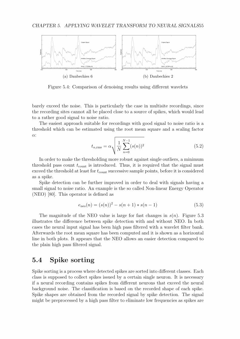
CHAPTER 5. APPLYING WAVELET TRANSFORM TO NEURAL SIGNALS55
550 555 560 565
Original Signal
MiniMaxi Denoised Signal
Noise 1.777658e+06
Time [ms]
Am
plitu
de
(a) Daubechies 6
550 555 560 565
Original Signal
MiniMaxi Denoised Signal
Noise 1.947081e+06
Time [ms]
Am
plitu
de
(b) Daubechies 2
Figure 5.4: Comparison of denoising results using different wavelets
barely exceed the noise. This is particularly the case in multisite recordings, sincethe recording sites cannot all be placed close to a source of spikes, which would leadto a rather good signal to noise ratio.
The easiest approach suitable for recordings with good signal to noise ratio is athreshold which can be estimated using the root mean square and a scaling factorα:
tα,rms = α
√√√√ 1
N
N−1∑n=0
(s(n))2 (5.2)
In order to make the thresholding more robust against single outliers, a minimumthreshold pass count tcount is introduced. Thus, it is required that the signal mustexceed the threshold at least for tcount successive sample points, before it is consideredas a spike.
Spike detection can be further improved in order to deal with signals having asmall signal to noise ratio. An example is the so called Non-linear Energy Operator(NEO) [80]. This operator is defined as
eneo(n) = (s(n))2 − s(n+ 1) ∗ s(n− 1) (5.3)
The magnitude of the NEO value is large for fast changes in s(n). Figure 5.3illustrates the difference between spike detection with and without NEO. In bothcases the neural input signal has been high pass filtered with a wavelet filter bank.Afterwards the root mean square has been computed and it is shown as a horizontalline in both plots. It appears that the NEO allows an easier detection compared tothe plain high pass filtered signal.
5.4 Spike sorting
Spike sorting is a process where detected spikes are sorted into different classes. Eachclass is supposed to collect spikes issued by a certain single neuron. It is necessaryif a neural recording contains spikes from different neurons that exceed the neuralbackground noise. The classification is based on the recorded shape of each spike.Spike shapes are obtained from the recorded signal by spike detection. The signalmight be preprocessed by a high pass filter to eliminate low frequencies as spikes are
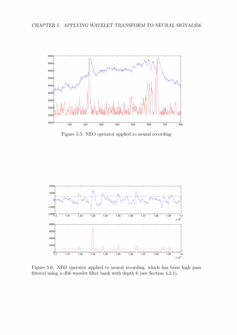
CHAPTER 5. APPLYING WAVELET TRANSFORM TO NEURAL SIGNALS56
100 200 300 400 500 600 700 8002000
2500
3000
3500
4000
4500
5000
5500
6000
6500
Figure 5.5: NEO operator applied to neural recording
1.3 1.31 1.32 1.33 1.34 1.35 1.36 1.37 1.38 1.39 1.4x 10⁴
−2000
−1000
0
1000
2000
1.3 1.31 1.32 1.33 1.34 1.35 1.36 1.37 1.38 1.39 1.4x 10⁴
0
2000
4000
6000
8000
Figure 5.6: NEO operator applied to neural recording, which has been high passfiltered using a db6 wavelet filter bank with depth 6 (see Section 4.2.1).

CHAPTER 5. APPLYING WAVELET TRANSFORM TO NEURAL SIGNALS57
in the frequency range from 500 Hz to 8 kHz. A second preprocessing step could bea denoising as described above in Section 5.2.
Spike sorting algorithms assume that the recorded versions of spikes issued bya single neuron have a characteristic shape. In principle, that is correct. However,several parameters influence the spike shape and the actual recorded version. Therecan be artefacts due to a moving electrode, or a changed position of the electrodeor the tissue might move. Sometimes pulse artefacts disturb the recording. Fur-thermore, the spike shape depends also on the previous activity of the respectiveneuron. A neuron which is firing spikes rapidly in so called bursts produces spikeswith changing shape, because the amplitude decreases and the width increases. Theactivity of two neighbouring neurons could overlap and cancel each other out. Also,the shape of spikes issued by two similar neurons might be also quite similar, so thatthey cannot be sorted into separate groups. With respect to these difficulties it isnot possible to provide a spike sorting algorithm which works reliable in all cases.A whole lot of methods have been proposed and a review of some methods can befound in [69].
Basically, spike sorting is performed in two steps. The first step is the featurecomputation and the second step is the classification. Usually finding the discrim-inating features of the spike shapes is the main problem. Having found good dis-criminating features a simple clustering method like e.g. the k-means algorihm [41]suffices for the second step. The result of the sorting can be visually supervisedeasily, if the used features form distinct clusters in feature space.
When selecting a method for spike feature computation the experimental settingmust be considered. If the probe has recording sites, which are very close to eachother, these pick up similar but not equal signals. The differences are due to slightlydifferent relative positions of the emitting neurons and the recording sites. Withsuch probes multiple shapes for the same spike are obtained and the differencesamong these shapes can serve as features. In [40] the spike sorting performanceusing recordings from single electrodes, stereotrodes, and tretrodes are compared.They found that it improves the more recording sites are used, i.e. tetrodes arebetter than stereotrodes, which in turn are better than single electrodes.
Some of the fork shaped silicon probes described in Section 6.1.1 (e.g. U3) featurea layout where the recording sites are placed in pairs such that they effectively workas multiple stereotrodes. If these probes are used, stereotrode specific spike featurescan be utilized for the spike sorting. In other designs the recording sites are placedso far apart from each other, that they do not pick up spikes from the same neurons.In this case the signal from each recording site must be treated like a single electroderecording.
5.4.1 Spike features
The starting point for spike feature computation is usually a set of spike shapesextracted from a neural recording. Some commonly used features in time domaininclude for instance:
• Minimum amplitude,

CHAPTER 5. APPLYING WAVELET TRANSFORM TO NEURAL SIGNALS58
• Maximal amplitude,
• Peak to peak amplitude,
• Temporal distance between minimum and maximal peak, and
• Temporal distance between zero crossings.
These simple descriptive features work quite well for neural recordings wherethe spikes have large amplitudes, with high signal to noise ratio. However, theyreduce the full shape of spike to certain keypoints which might not be significant fordiscrimination. In general it is better to consider the complete shape of the spikes fordiscrimination. A widely used approach is to use the principal component analysisin order to find the discriminating features for a given set of spike shapes. Thisapproach is outlined in Section 5.4.2. However, the principal component analysisfails to classify overlapping spikes correctly. In best case these fall into a separateclass which collects all unspecific spike shapes.
Another approach which also accounts for the full shapes is based on Bayesianmodeling of the spikes [68]. At this a probabilistic model for the neural recording isdefined to compute the probability of both form and number of spike shapes. Fur-thermore, according to [68] the Bayesian approach is also able to analyse overlappingspike shapes.
Other approaches utilize wavelet based time frequency analysis in order to obtaindiscriminative features [67, 53]. In [67] a wavelet based approach is compared withprincipal component analysis (PCA, see Section 5.4.2) and reduced feature set (RFS,[88]), which are alternative methods to obtain features for spike shapes. In thedescribed setting the wavelet based approach outperforms PCA and RFS. The spikeshapes are decomposed by a dyadic wavelet filter bank. Then the sets of coefficientswith largest mean value and largest standard deviation and – most preferable –having a bimodal or multimodal distribution over the population of spike shapesare selected manually by visual inspection. The classification is done manuallythrough a software interface which allows to delimit the clusters interactively.
The approach in [53] utiltizes a wavelet packet decomposition. This transformdivides the frequency space into bands of equal width, the so-called wavelet packets,allowing a better localization in frequency than the wavelet decomposition. A setof wavelet packets is selected by using e.g. the best basis algorithm with Shannon’sinformation cost function and is used for detection and spike sorting. Accordingto [53] this method is more efficient both in separating spikes from noise and inresolving overlapping spikes than methods like PCA and wavelet decomposition.
5.4.2 Principal component analysis
The spikes are extracted from the original signal by spike detection and then alignedin time for example by aligning their maximum amplitude. As an optimization itis possible to perform an upsampling of the extracted spike snippets in order toalign them more precisely, then the alignment resolution can be higher than theactual sampling resolution. For principal component analysis (PCA) each spike
CHAPTER 5. APPLYING WAVELET TRANSFORM TO NEURAL SIGNALS59
snippet is regarded as a feature vector. We define a matrix A which rows containthe feature vectors, i.e. the spike snippets. Each column in matrix A representsa variable in feature space. The PCA computes the eigenvectors and eigenvaluesof the covariance matrix of A. They are sorted with respect to the magnitude ofthe eigenvalues which corresponds to the variance of variables in the orignal featurespace, i.e. the first principal component vector represents the variables with thelargest variance. The PCA results in a new basis for the feature space, which allowsa compact representation of the feature vectors. The first few, i.e. three or four,coefficients of the new representation are the new feature values, thus the PCA hasreduced the dimensionalty to three or four dimensions. Using these feature values,standard clustering methods can be applied to separate different classes of spikesnippets.
The PCA requires the complete set of feature vectors to be available. Therefore,it is not well suited for online feature computation.
5.4.3 Online wavelet based spike sorting
The online wavelet based spike sorting is supposed to classify the spikes immediatelyafter acquisition, in order to give the experimenter a direct feedback about thecontents of the recorded signals. At the time of classification the complete signalis not available. This prevents us to utilized some classification methods, whichrequire the complete signals containing the spikes, which shall be classified, as forinstance the principal component method. Instead the signal is decomposed by awavelet filter bank and the wavelet coefficients are used to compute feature vectors.
Given the wavelet based approach there are two main problems to deal with, i.e.translation variance and quantization errors, which are the subject of the followingparagraphs.
Translation variance
Figure 5.7 reveals the most prominent problem using wavelet based features forclassification if the spike snippets are not aligned. Figure 5.7(a) shows the sameexemplary spike snippet at two different positions relative to the wavelet decompo-sition raster which is indicated by the vertical dotted lines. The red (right hand) isdelayed by 0.26 ms versus the blue (left hand) spike, which corresponds to 13 samplepoints at 50 kHz. The scalograms in Figure 5.7(c) and Figure 5.7(d) illustrate thetranslation variance in a direct comparison of the wavelet coefficients resulting froma decompositin with the Daubechies 3 wavelet. A scalogram indicates the magnitudeof the wavelet coefficients in a two dimensional plot. The different scales are plottedversus the time on y- and x-axis, respectively. The coefficents magnitude is mappedonto a color according to the given colorbar. The white line in the scalogram plotsindicates the reference position of the detected spike. A comparision of the valuesin level 3 for instance reveals a large difference although both spike only differ intheir relative position to the decomposition raster. Consequently the translationvariance leads to great differences in the final feature space. For Figure 5.7(b) thefeature values have been computed as the absolute sum of the wavelet coefficients

CHAPTER 5. APPLYING WAVELET TRANSFORM TO NEURAL SIGNALS60
(a) Spike snippets (b) Absolute sum of wavelet coefficients
(c) Scalogram of blue spike (d) Scalogram of red spike
Figure 5.7: Spike snippets, wavelet based features, and scalograms of the same singlespike snippet at different translations
within the different levels. Here the levels 2 and 3 are plotted versus each other.They have been computed based on different wavlets as indicated in the legend ofFigure 5.7(b) for the same spike snippet at eight different translations. Ideally, themarks with the same symbol should be located at the same point in feature space,because they all represent the same spike. However, this is not the case. Insteadthey are spread over a large range of values. Thus, a precise classification based onthese feature values is hardly possible. Only spikes that differ a lot in time domain,can be separated by these feature values.
In order to handle the translation variance problem, we need an exact referenceposition in time domain to determine the shift of the spike with respect to thedecomposition raster. Therefore, the spikes are detected in time domain using the

CHAPTER 5. APPLYING WAVELET TRANSFORM TO NEURAL SIGNALS61
0 10 20 30 40 50 60 700
0.1
0.2
0.3
0.4level=3
ener
gy
0 10 20 30 40 50 60 700
0.2
0.4
0.6
0.8level=4
ener
gy
0 10 20 30 40 50 60 700
0.2
0.4
0.6
0.8level=5
ener
gy
delta featuresspike features
Figure 5.8: Translation variance of the energy feature
NEO operator (see also Section 5.3), as it turns out that a robust detection of theexact reference position in wavelet domain does not work well. This is because of thecoarse time resolution in frequency bands where the spikes lead to large coefficients.
Generally, the translation variance of a dyadic filter bank is periodic with periodM , i.e. it is translation invariant for translations n and n + M . The period Mdepends on the decomposition depth L as M = 2L. Therefore, there are M differentdecomposition variants for a given signal s(n). Two approaches were examined totackle the translation variance problem:
1. Normalization of translation variant wavelet coefficients
Compute all M decomposition variants of a fixed normalization signal s(n) =δ(n). So for each translation m = 0, . . . ,M − 1 we have a decompositionvariant Dm. Given the reference position p of a spike we can determine thecorresponding decomposition variant Dm,m = p mod M , which contains thenormalization coefficients.
Figure 5.8 shows the distribution of energy over three different levels of thewavelet decomposition using the δ function and a spike template as input sig-nal. 64 instances of both δ function and spike template have been decomposedby a Daubechies wavelet with 6 vanishing moments into 6 detail levels. Theinstances were all shifted differently against the decomposition raster. The

CHAPTER 5. APPLYING WAVELET TRANSFORM TO NEURAL SIGNALS62
respective shift is indicated on the X-axis. The energy distribution varies pe-riodically, where the period depends on the decomposition level l with 2l. Theenergy of the spike template has been normalized to one. However, the fig-ure reveals that there is no systematic translation dependent variation of theenergy distribution over different decomposition levels. Therefore, it appearsimpossible to utilize the energy distribution of the δ function to normalize thetranslation variant decomposition of a given spike instance.
2. Translation dependent classification
The classification is done with respect to the translation, i.e. only spikes withthe same translation are compared with each other. Thus, the classificationis translation invariant, but this results in a separate feature space for eachtranslation Rm,m = 0, . . . ,M − 1. Each feature space contains cluster whichmust be mapped onto each other.
For a classification with a training dataset this mapping is easy, since theclasses of the cluster in Rm are known a priori. For automatic classificationwithout training data, we must find the corresponding clusters C0 in Rm0 andC1 in Rm1 . This could be achieved by calculation of the mean spike in clus-ter C0, which is then transformed into the feature space Rm1 by translationand wavelet decomposition. The corresponding cluster C1 is the cluster whichis next should be the desired cluster. However, it is possible that for cer-tain translations two cluster overlap, making it impossible to find a suitablemapping and then the classification problem cannot be solved.
Approaches to overcome the translation variance problem are described in [7].The simplest solution is to use an undecimated variant of the wavelet transform,which is called the algorithme a trous [73]. This algorithm is very similar to the fastwavelet transform. The only difference is, that instead of sub-sampling the datathe wavelet filter are dilated by insertion of zeroes. This leads to shift invariantcoefficients, but at the cost of an increased computational complexity regarding op-erations as well as memory usage which depends on the depth of the decomposition.
Another approach is the dual-tree complex wavelet transform (DTCWT), whichwas introduced with [63] and for which [92] gives an elaborated overview. TheDTCWT is an enhancement of the traditional real wavelet transform. In particular,it is approximately shift invariant while it can be implemented based on the samedecomposition and reconstruction algorithms as the traditional wavelet transform.As it uses two decompositon filter banks it needs about 2 times more operations andalso 2 times more memory resources for the result. The wavelets in the two treesare Hilbert transforms of each other [92], i.e. they are 90 out of phase. Therefore,the wavelet coefficients from both decomposition trees interpolate each other. Asingle complex wavelet coefficient is composed from the two corresponding real valuewavelet coeffiecients from both trees. Furthermore, the use of two trees reduces theeffect of the subsampling, i.e. aliasing is greatly attenuated. The method relies onspecially designed wavelets in order to achieve the shift invariance. It is not possibleto just use e.g. the standard Daubechies wavelets.

CHAPTER 5. APPLYING WAVELET TRANSFORM TO NEURAL SIGNALS63
Quantization errors
Massive quantization errors occur if a 16 bit input signal is decomposed into 16 bitinteger wavelet coefficients. The method introduced in Section 4.3.2 adds a roundingto each lifting step, i.e. in each lifting step a quantization error occurs. These errorssum up to a large error. Changing the scale factor as the final step of the lifting inorder to avoid 16 bit overflows also increases the quantization error. A solution is todouble the precision for the wavelet coefficients and use 32 bit floating point values.The drawback is, that the wavlet coefficients need twice as much space.
Chapter 6
Data Acquisition System
6.1 Hardware
The VSAMUEL data acquisition system [32, 43] consists of several components.Figure 6.1 gives an overview in case of 128 channel recording setup. Signals areacquired with multichannel probes in the nervous tissue. The small amplitude ofthese signals is amplified in a preamplifier stage which has a gain of 16 (24 dB) perchannel. It uses a battery as DC power supply. The preamplified signals are routedthrough the battery pack to the main amplifier which resides outside the recordingarea in a 19 inch rack together with the data acquisition host. The main amplifierhas ten individual gain settings per channel. Both amplifier stages together providegains ranging between 80 and 80,000 times. The data acquisition host has eightAD16 boards which are in turn mounted on four M67 boards. Each analog channelhas an own analog to digital converter which resides on one of the AD16 boards.Analog digital conversion is possible with rates between 5 kHz and 50 kHz at 16 bitresolution. The CPU on the M67 board performs some signal processing tasks beforethe data is sent to the host CPU were it is visualized and stored to hard disk.
6.1.1 Probes
The probes are manufactured by Acreo AB (Kista, Sweden) using micro structuretechnology as described in Section 3.5. Basically they are fork shaped silicon withlinearly arranged recording sites on each shaft. With respect to different targetareas, there are several different probe layouts. As a first step probes with 32 siteswere developed. Figure 6.1 summarizes the technical data of the eight designs andFigure 6.2 shows exemplarily the design of the E3 probe. In a second step thenumber of recording sites was increased to 64. Some 64 channel probe designs areidentical to the 32 channel version but with double recording sites. Table 6.2 givean overview of the different specifications. Figure 6.3(a) for instance shows a probespecially designed for recording from cerebellum. It has double recording sites on4 mm shafts, where the recording site spacing of 200 µm between the three doublerecording sites next to the shaft tips and a 100 µm between the third and the fourthdouble recording site. It covers the Purkinje cell layer and the molecular layer withdense spacing and has a wider spacing to cover the granular and medullary layer
64
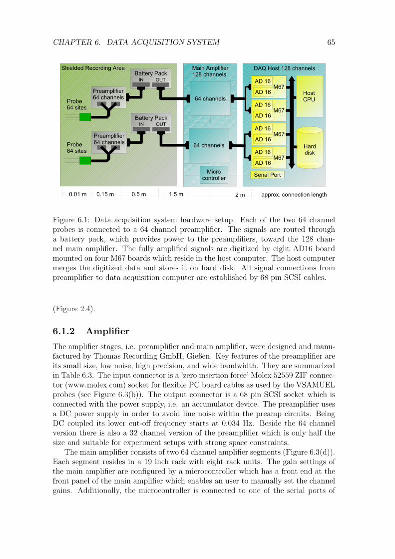
CHAPTER 6. DATA ACQUISITION SYSTEM 65
Shielded Recording Area
Preamplifier64 channels
Main Amplifier128 channels
DAQ Host 128 channels
64 channels
64 channels
Battery PackOUTIN
Probe64 sites
Battery PackOUTIN
Preamplifier64 channelsProbe
64 sites
M67 AD 16
AD 16 Host CPU
Harddisk
M67 AD 16
AD 16
M67 AD 16
AD 16
M67 AD 16
AD 16
Serial PortMicrocontroller
0.01 m 0.15 m 0.5 m 1.5 m 2 m approx. connection length
Figure 6.1: Data acquisition system hardware setup. Each of the two 64 channelprobes is connected to a 64 channel preamplifier. The signals are routed througha battery pack, which provides power to the preamplifiers, toward the 128 chan-nel main amplifier. The fully amplified signals are digitized by eight AD16 boardmounted on four M67 boards which reside in the host computer. The host computermerges the digitized data and stores it on hard disk. All signal connections frompreamplifier to data acquisition computer are established by 68 pin SCSI cables.
(Figure 2.4).
6.1.2 Amplifier
The amplifier stages, i.e. preamplifier and main amplifier, were designed and manu-factured by Thomas Recording GmbH, Gießen. Key features of the preamplifier areits small size, low noise, high precision, and wide bandwidth. They are summarizedin Table 6.3. The input connector is a ’zero insertion force’ Molex 52559 ZIF connec-tor (www.molex.com) socket for flexible PC board cables as used by the VSAMUELprobes (see Figure 6.3(b)). The output connector is a 68 pin SCSI socket which isconnected with the power supply, i.e. an accumulator device. The preamplifier usesa DC power supply in order to avoid line noise within the preamp circuits. BeingDC coupled its lower cut-off frequency starts at 0.034 Hz. Beside the 64 channelversion there is also a 32 channel version of the preamplifier which is only half thesize and suitable for experiment setups with strong space constraints.
The main amplifier consists of two 64 channel amplifier segments (Figure 6.3(d)).Each segment resides in a 19 inch rack with eight rack units. The gain settings ofthe main amplifier are configured by a microcontroller which has a front end at thefront panel of the main amplifier which enables an user to manually set the channelgains. Additionally, the microcontroller is connected to one of the serial ports of

CHAPTER 6. DATA ACQUISITION SYSTEM 66
w = 25µm
2000µm
a = 200µm
L = 5000µm
b = 200µm
210µm
2110µm
1875µm
75µm
Figure 6.2: Design of the VSAMUEL probe E3 as described in [82]. The recordingsites of this probe span a regular two dimensional with equidistant spacing of 200 µmalong both dimensions.
Designname
Number of shaftsand sites
Shaftlength(L) µm
Site c/cdistance(a) µm
Shaftc/cdistance(b) µm
Shaft widthat active re-gion (w) µm
M1 1 shaft × 32 sites 7000 50 – Increasingfrom 0 to100
M2 5 shaft × 6 sites 10000 250 500 25E1 4 shaft × 8 sites 5000 100 400 25E2 8 shaft × 4 sites 4000 200,
200, 100200 25
E3 8 shaft × 4 sites 4000 200 200 25K1 4 shaft × 8 sites 15000 100 500 25U1 4 shaft × 8 sites 10000 100 250 25U2 4 shaft × 8 sites 5000 50 60 25
Table 6.1: Specification of VSAMUEL probes with 32 recording sites. Shaft lengthL, site center/center distance a, shaft center/center distance (b) and shaft width atactive region w are drawn into Figure 6.2.
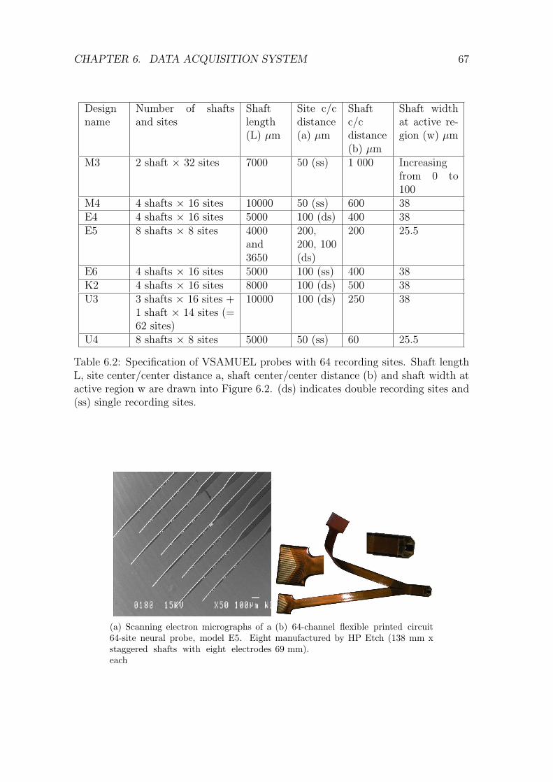
CHAPTER 6. DATA ACQUISITION SYSTEM 67
Designname
Number of shaftsand sites
Shaftlength(L) µm
Site c/cdistance(a) µm
Shaftc/cdistance(b) µm
Shaft widthat active re-gion (w) µm
M3 2 shaft × 32 sites 7000 50 (ss) 1 000 Increasingfrom 0 to100
M4 4 shafts × 16 sites 10000 50 (ss) 600 38E4 4 shafts × 16 sites 5000 100 (ds) 400 38E5 8 shafts × 8 sites 4000
and3650
200,200, 100(ds)
200 25.5
E6 4 shafts × 16 sites 5000 100 (ss) 400 38K2 4 shafts × 16 sites 8000 100 (ds) 500 38U3 3 shafts × 16 sites +
1 shaft × 14 sites (=62 sites)
10000 100 (ds) 250 38
U4 8 shafts × 8 sites 5000 50 (ss) 60 25.5
Table 6.2: Specification of VSAMUEL probes with 64 recording sites. Shaft lengthL, site center/center distance a, shaft center/center distance (b) and shaft width atactive region w are drawn into Figure 6.2. (ds) indicates double recording sites and(ss) single recording sites.
(a) Scanning electron micrographs of a64-site neural probe, model E5. Eightstaggered shafts with eight electrodeseach
(b) 64-channel flexible printed circuitmanufactured by HP Etch (138 mm x69 mm).
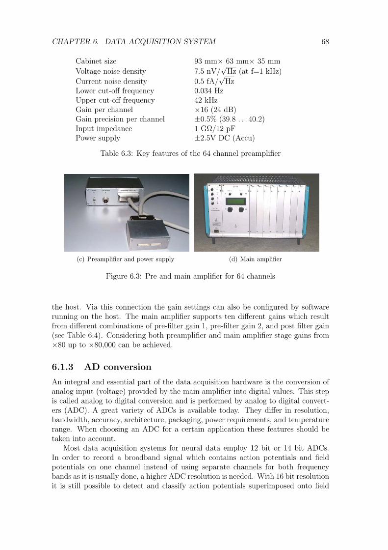
CHAPTER 6. DATA ACQUISITION SYSTEM 68
Cabinet size 93 mm× 63 mm× 35 mm
Voltage noise density 7.5 nV/√
Hz (at f=1 kHz)
Current noise density 0.5 fA/√
HzLower cut-off frequency 0.034 HzUpper cut-off frequency 42 kHzGain per channel ×16 (24 dB)Gain precision per channel ±0.5% (39.8 . . . 40.2)Input impedance 1 GΩ/12 pFPower supply ±2.5V DC (Accu)
Table 6.3: Key features of the 64 channel preamplifier
(c) Preamplifier and power supply (d) Main amplifier
Figure 6.3: Pre and main amplifier for 64 channels
the host. Via this connection the gain settings can also be configured by softwarerunning on the host. The main amplifier supports ten different gains which resultfrom different combinations of pre-filter gain 1, pre-filter gain 2, and post filter gain(see Table 6.4). Considering both preamplifier and main amplifier stage gains from×80 up to ×80,000 can be achieved.
6.1.3 AD conversion
An integral and essential part of the data acquisition hardware is the conversion ofanalog input (voltage) provided by the main amplifier into digital values. This stepis called analog to digital conversion and is performed by analog to digital convert-ers (ADC). A great variety of ADCs is available today. They differ in resolution,bandwidth, accuracy, architecture, packaging, power requirements, and temperaturerange. When choosing an ADC for a certain application these features should betaken into account.
Most data acquisition systems for neural data employ 12 bit or 14 bit ADCs.In order to record a broadband signal which contains action potentials and fieldpotentials on one channel instead of using separate channels for both frequencybands as it is usually done, a higher ADC resolution is needed. With 16 bit resolutionit is still possible to detect and classify action potentials superimposed onto field

CHAPTER 6. DATA ACQUISITION SYSTEM 69
Cabinet size 16 RU × 19 inch × d cm
Voltage noise density 21 nV/√
Hz (@ Gain=5k,BW=16kHz)
Lower cut-off frequency 0.060 HzUpper cut-off frequency 16 kHzPre-filter gain 1 ×1, ×2, ×5, ×10Pre-filter gain 2 ×1, ×10, ×100Post filter gain ×5Total gain ×5, ×10, ×25, ×50, ×100, ×250,
×500, ×1000, ×2500, ×5000Gain precision ±1.5%CMRR 114 dB(@f=1kHz)Input impedance 2.2 MΩ/10 pFPower supply integrated
Table 6.4: Main amplifier features
potentials, while 12 bit or 14 bit are not sufficient. Thus, the VSDAQ systememploys 16 bit ADCs.
For sake of simplicity we overestimate the maximum peak to peak amplitudeof action and field potentials and suppose that their values are about 200mV and4000mV, respectively. Therefore, with 12 bit AD conversion the resolution is about1mV per bit, while 16 bit AD conversion results in 0.06mV per bit. In the 12 bitcase the action potential are effectively sampled with 7.6 bit, while we have 11.7 bitin the 16 bit case.
The most popular ADC architectures include [5]:
• successive approximation (SAR) – a successive approximations shift registeris the key defining element,
• flash – all decisions are made simultaneously,
• pipelined – multiple flash stages.
• sigma-delta (Σ∆) – a charge-balancing type
These architectures mainly differ with respect to number of comparators andnumber of comparison cycles. The plain flash architecture requires one comparatorfor each digital output value, e.g. a 4 bit flash ADC requires 16 comparators. Itcan convert an analog input within a single cycle. This architecture is not suitablefor high resolutions, as it requires e.g. 216 = 65, 535 comparators in case of a 16 bitADC. The number of comparators can be reduced when using cascaded flash ADCs.This architecture is referred to as pipelined. Each stage can consist of a m bit flashADC and p such stages establish a n = m × p bit ADC, which only needs 2m × pcomparators. Sort of orthogonal to the flash architecture is the SAR architecture,which uses only a single comparator, but needs an additional cycle for each bit ofresolution.

CHAPTER 6. DATA ACQUISITION SYSTEM 70
ΣDigital Filter
andDecimator
1-BitDAC
∫
Integrator Comparator
Bit streamDAnalog Digital
-+
Figure 6.4: Basic concept of sigma-delta converter, [1]
In the VSDAQ system ADCs build according to the sigma-delta architecture,which takes another approach, are employed. Basically, it uses an integrator, acomparator, and a single bit DAC combined as shown in Figure 6.4.
Given a reference voltage Vref the output of the digital analog converter (DAC)is either −Vref or +Vref , depending on the comparator output, which is either 0 or1. The output of the DAC is subtracted from the input voltage Vin and the result isthe new input to the comparator. The comparator output is 1 or 0 for input voltagegreater or less than ground level, respectively. The output of the comparator is asequence of zeros and ones. This sequence represents the input voltage Vin in thefollowing matter: If Vin is closer to +Vref the sequence will contain more ones thanzeros and if Vin is closer to −Vref the sequence will contain more zeros than ones.With Vin being close to midscale the sequence will have approximately the samenumber of zeros and ones. A digital filter can be employed to obtain a sample valuefrom the sequence.
The ADC hardware used in the VSDAQ system is a set of so called AD16 boardsmanufactured by Innovative Integration. A single AD16 board features 16 sigma-delta ADCs (Analog Devices, AD7722), where each ADC is capable of sampling with16 bit resolution at a rate of 195.3kHz. In the VSDAQ system they are, however,used up to a rate of 50kHz. The analog input is continuously sampled by a sigma-delta modulator which eliminates the need for external sample-and-hold circuitry.The modulator output is processed by two FIR digital filters in series. Due to thison-chip filtering external antialias filters only need to be of first order. The filterintroduce a group delay of 215.5 µs. The ADCs within a single AD16 board aresynchronized such that data can be simultaneously acquired from all 16 channels.
The AD16 board has a 32 bit architecture, i.e. the smallest data unit whichcan be handled has 32 bits. As a consequence the 16 bit AD converters can onlybe enabled or disabled in pairs. Channel 0 and 1, 2 and 3, etc. form such a pair.However, these pairs can be controlled independently.
Conversion data is transferred from the ADC pairs into a First In First Out buffer(FIFO) on the AD16 board that can hold up to 512 samples or 256 samples pairs.The FIFO is connected to the DSP via a data bus on the M67 board (Omnibus).Additionally the FIFO uses one of the four external interrupt input lines of the DSP.

CHAPTER 6. DATA ACQUISITION SYSTEM 71
Figure 6.5: AD16 board
Figure 6.6: M67 board equipped with AD16 and its installed heat spreader
Via this interrupt line the FIFO notifies the DSP if its fill state exceeds a certainconfigurable threshold. The current 32 bit value of the FIFO is mapped into theDSP’s memory space. A read access on this location by the DSP or by its DMAcontroller causes the FIFO to put the current value on the bus, and afterwards theFIFO’s tail pointer is moved to the next value.
6.1.4 Digital signal processor board M67
The digital signal processor board M67 is manufactured by Innovative Integration(Thousand Oaks, California, USA). Its core is the Texas Instruments C6701 digitalsignal processor. In addition to the two on-chip timers is has three 16 bit timers inFPGA logic and a 32 direct digital synthesizer (DDS) timer from Analog Devices(AD9850). The board provides a modular IO expansion system, i.e. two slots forexpansion boards. In the VSDAQ system both slots are used by the AD16 boardwhich perform the analog digital conversion. With the digital IO port 32 bit of digitalinput or output are available. The board has JTAG hardware emulation support,which makes it possible to perform realtime debugging using Texas Instruments IDECode Composer Studio. The board interfaces with the host PC via the PCI bus,with a total bandwidth of 130 MB/s for fast digital data transfers. The M67 canperform busmaster transfers from or into a shared memory area on the host PC.
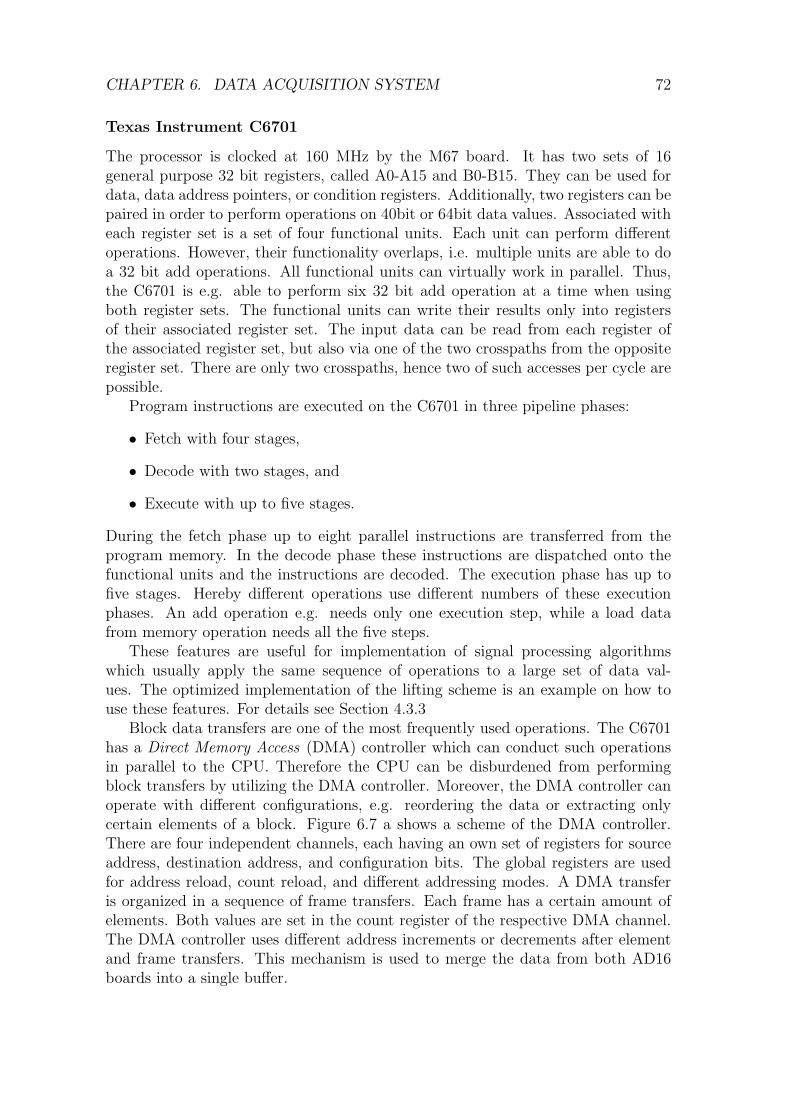
CHAPTER 6. DATA ACQUISITION SYSTEM 72
Texas Instrument C6701
The processor is clocked at 160 MHz by the M67 board. It has two sets of 16general purpose 32 bit registers, called A0-A15 and B0-B15. They can be used fordata, data address pointers, or condition registers. Additionally, two registers can bepaired in order to perform operations on 40bit or 64bit data values. Associated witheach register set is a set of four functional units. Each unit can perform differentoperations. However, their functionality overlaps, i.e. multiple units are able to doa 32 bit add operations. All functional units can virtually work in parallel. Thus,the C6701 is e.g. able to perform six 32 bit add operation at a time when usingboth register sets. The functional units can write their results only into registersof their associated register set. The input data can be read from each register ofthe associated register set, but also via one of the two crosspaths from the oppositeregister set. There are only two crosspaths, hence two of such accesses per cycle arepossible.
Program instructions are executed on the C6701 in three pipeline phases:
• Fetch with four stages,
• Decode with two stages, and
• Execute with up to five stages.
During the fetch phase up to eight parallel instructions are transferred from theprogram memory. In the decode phase these instructions are dispatched onto thefunctional units and the instructions are decoded. The execution phase has up tofive stages. Hereby different operations use different numbers of these executionphases. An add operation e.g. needs only one execution step, while a load datafrom memory operation needs all the five steps.
These features are useful for implementation of signal processing algorithmswhich usually apply the same sequence of operations to a large set of data val-ues. The optimized implementation of the lifting scheme is an example on how touse these features. For details see Section 4.3.3
Block data transfers are one of the most frequently used operations. The C6701has a Direct Memory Access (DMA) controller which can conduct such operationsin parallel to the CPU. Therefore the CPU can be disburdened from performingblock transfers by utilizing the DMA controller. Moreover, the DMA controller canoperate with different configurations, e.g. reordering the data or extracting onlycertain elements of a block. Figure 6.7 a shows a scheme of the DMA controller.There are four independent channels, each having an own set of registers for sourceaddress, destination address, and configuration bits. The global registers are usedfor address reload, count reload, and different addressing modes. A DMA transferis organized in a sequence of frame transfers. Each frame has a certain amount ofelements. Both values are set in the count register of the respective DMA channel.The DMA controller uses different address increments or decrements after elementand frame transfers. This mechanism is used to merge the data from both AD16boards into a single buffer.

CHAPTER 6. DATA ACQUISITION SYSTEM 73
Global Configuration Registers
Address A
Address C
Address D
Address BDMA Channel configuration registersChannel 0 – 3
Primary Control
Secondary Control
Source Address
Destination Address
Element CountFrame Count
DMA Controller Configuration
Count A
Count B
Index A
Index B
Figure 6.7: DMA controller configuration registers
The data acquisition board for 32 channels is shown in Figure 6.6 and anschematic overview in Figure 6.8. The M67 board is equipped with two AD16boards. The AD16 boards are synchronized with the AdcSync cable (see also Ap-pendix B.2). Data acquired by AD16 boards is stored in the respective FIFO andafter a certain amount of samples are acquired each AD16 board triggers an in-terrupt which in turn initiates a DMA transfer which transports the data into theinternal RAM of the DSP. If required the data can be processed and afterwardsanother DMA transfer copies the data into ASRAM. From ASRAM the data can betransported into a shared memory section on the host PC. This transfer is conductedby a separate controller which works independent from both host CPU and DSPboard CPU. A finished transfer is signaled by interrupts. Note, that transfers fromAD16 to DSP and from DSP to ASRAM both use the same bus, i.e. they cannot beperformed simultaneously. This is taken into account, by triggering transfers intoASRAM, just after a transfer from AD16 boards has finished. This way there is nosimultaneous usage of the bus and all transfers can be performed as fast as possible.
6.1.5 Synchronization
There are two means of synchronization one for the M67 boards and one for the AD16boards. Multiple M67 boards are synchronized with a master-slave mechanism. Themaster board provides its clock signals to the other boards, i.e. the slave boards.Hereby the slave boards are connected to a clock bus, which is driven by the masterboard. For details refer to [56] or Appendix B.1. Since the ADCs on the AD16board are driven by a clock with 128 times the sampling rate, the transmitted clockrate is about 6 MHz. The other synchronization is necessary among the ADCs of theAD16 boards. Each AD16 board provides a SyncIn pin and a SyncOut pin these.We connect SyncOut of AD16 board 0 with SynIn of AD16 board 1, and continue
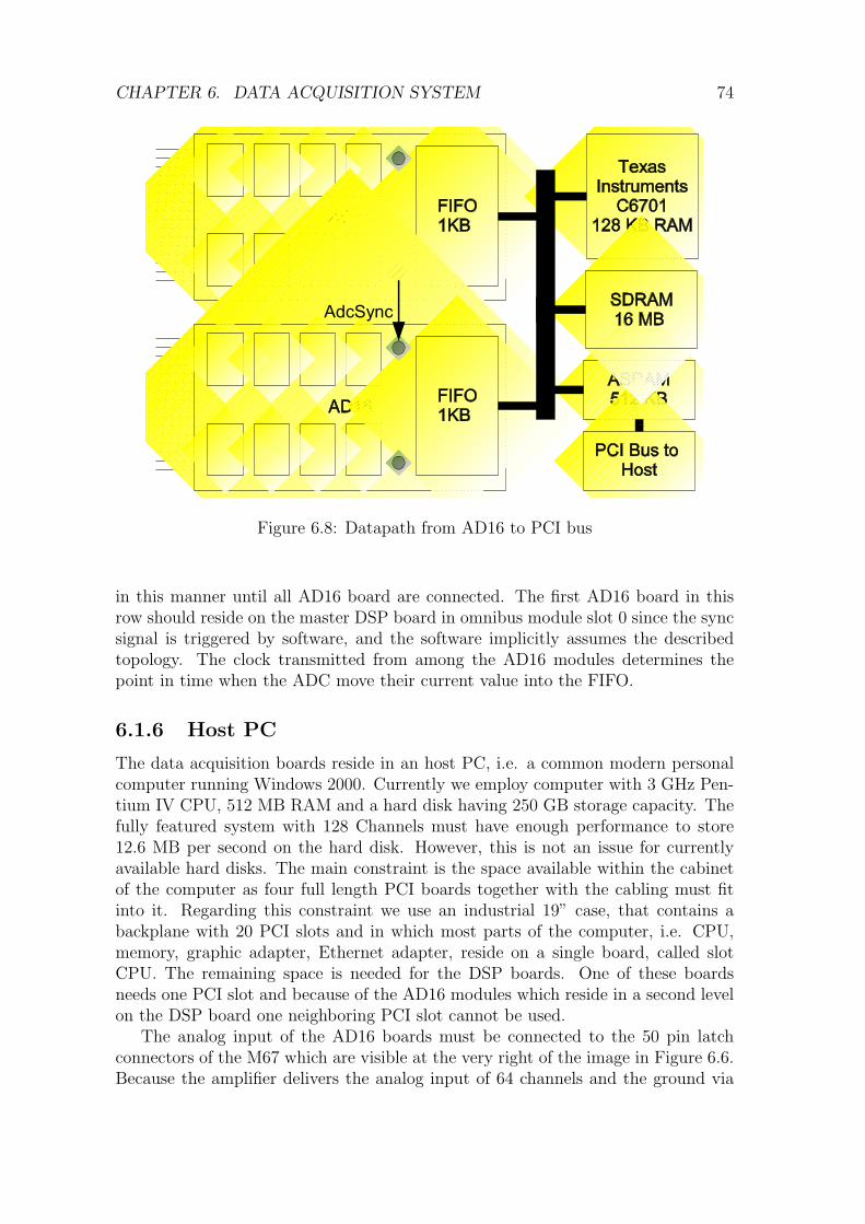
CHAPTER 6. DATA ACQUISITION SYSTEM 74
Figure 6.8: Datapath from AD16 to PCI bus
in this manner until all AD16 board are connected. The first AD16 board in thisrow should reside on the master DSP board in omnibus module slot 0 since the syncsignal is triggered by software, and the software implicitly assumes the describedtopology. The clock transmitted from among the AD16 modules determines thepoint in time when the ADC move their current value into the FIFO.
6.1.6 Host PC
The data acquisition boards reside in an host PC, i.e. a common modern personalcomputer running Windows 2000. Currently we employ computer with 3 GHz Pen-tium IV CPU, 512 MB RAM and a hard disk having 250 GB storage capacity. Thefully featured system with 128 Channels must have enough performance to store12.6 MB per second on the hard disk. However, this is not an issue for currentlyavailable hard disks. The main constraint is the space available within the cabinetof the computer as four full length PCI boards together with the cabling must fitinto it. Regarding this constraint we use an industrial 19” case, that contains abackplane with 20 PCI slots and in which most parts of the computer, i.e. CPU,memory, graphic adapter, Ethernet adapter, reside on a single board, called slotCPU. The remaining space is needed for the DSP boards. One of these boardsneeds one PCI slot and because of the AD16 modules which reside in a second levelon the DSP board one neighboring PCI slot cannot be used.
The analog input of the AD16 boards must be connected to the 50 pin latchconnectors of the M67 which are visible at the very right of the image in Figure 6.6.Because the amplifier delivers the analog input of 64 channels and the ground via
CHAPTER 6. DATA ACQUISITION SYSTEM 75
Figure 6.9: Host PC of data acquisition system with 128 channels. On the left youfind the slot CPU, and the other four boards on the right are the data acquisitionboards. At the bottom the SyncClockLink cable which synchronizes the boards andat the top the additional fans are visible.
68 pin SCSI cable an appropriate adapter board is needed. Figure 6.10 shows thisboard, which is called ScsiToLatch board. The 64 input channels are distributedto the four latch connectors, i.e. 16 channels on each latch connector, which mustbe connected with the respective connectors on the M67 boards using a 1 to 1 50pin ribbon cable. Since the AD converter of the AD16 board need differential inputthere is a negative and a positive input pin for each AD converter. The ScsiToLatchboard connects all negative input pins to ground and the positive input pins to theactual analog input channel. The SCSI connector has 4 lines with ground whichare separately mapped to the four latch connectors. Thus, it is possible to providedifferent ground levels to for each block of 16 channels. However, with the jumperson the ScsiToLatch board all ground lines can be connected in order to make surethat they are equal.
6.1.7 Thermal issues
In a series of test runs it appeared that the AD16 modules have a thermal problem.We tested different combinations of M67 boards equipped with two AD16 modules:
• Combination A with M67 board G274, AD16 modules B145-1 and B138
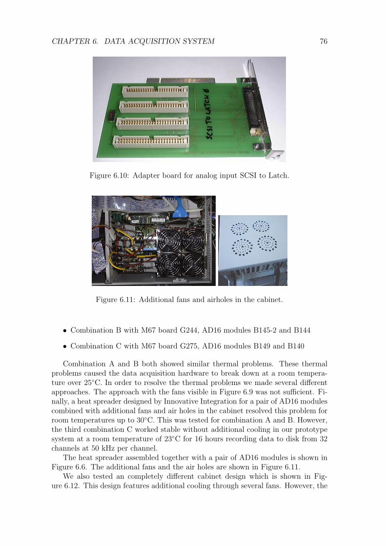
CHAPTER 6. DATA ACQUISITION SYSTEM 76
Figure 6.10: Adapter board for analog input SCSI to Latch.
Figure 6.11: Additional fans and airholes in the cabinet.
• Combination B with M67 board G244, AD16 modules B145-2 and B144
• Combination C with M67 board G275, AD16 modules B149 and B140
Combination A and B both showed similar thermal problems. These thermalproblems caused the data acquisition hardware to break down at a room tempera-ture over 25C. In order to resolve the thermal problems we made several differentapproaches. The approach with the fans visible in Figure 6.9 was not sufficient. Fi-nally, a heat spreader designed by Innovative Integration for a pair of AD16 modulescombined with additional fans and air holes in the cabinet resolved this problem forroom temperatures up to 30C. This was tested for combination A and B. However,the third combination C worked stable without additional cooling in our prototypesystem at a room temperature of 23C for 16 hours recording data to disk from 32channels at 50 kHz per channel.
The heat spreader assembled together with a pair of AD16 modules is shown inFigure 6.6. The additional fans and the air holes are shown in Figure 6.11.
We also tested an completely different cabinet design which is shown in Fig-ure 6.12. This design features additional cooling through several fans. However, the

CHAPTER 6. DATA ACQUISITION SYSTEM 77
Figure 6.12: Small cabinet with improved air flow due to multiple fans withM67/AD16 board equipped with heat spreader
combination A worked not stable in this cabinet, i.e. the data acquisition stoppedafter 30 minutes at a room temperature about 24 Celcius. Instead, the combina-tion B which does not have heatspreader worked stable over 18 hours at a roomtemperature at about 32 Celcius.
Our tests lead to the conclusion that the thermal stability of AD16 modulesdiffers individually, which in turn means that the thermal behaviour of each AD16module should be checked, before being used in a productive system. This seems tobe custom for most PC-Systems and is called burn-in.
6.2 Software
The data acquisition software has two parts: a DSP application and a host applica-tion. The DSP application executes on the DSP boards, while the host applicationruns on the host PC. Both applications were implemented using an appropriate in-tegrated development environments (IDE), i.e. Texas Instruments Code ComposerStudio for the DSP application and Borland C++ Builder for the host application.Both IDEs run under Windows NT/2000 and provide project management, com-pilation, and execution/debugging interface. The DSP application is based on theDSP/Bios real time operating system, while the host application employs BorlandsVisual Component Library (VCL) which encapsulates Windows API functions andWindows standard controls and dialogs.
6.2.1 DSP application
Being executed on the M67 board the DSP application is virtually invisible for theuser. It is transparently configured and started by the host application and performsthe following major tasks:
• Data acquisition
• Processing
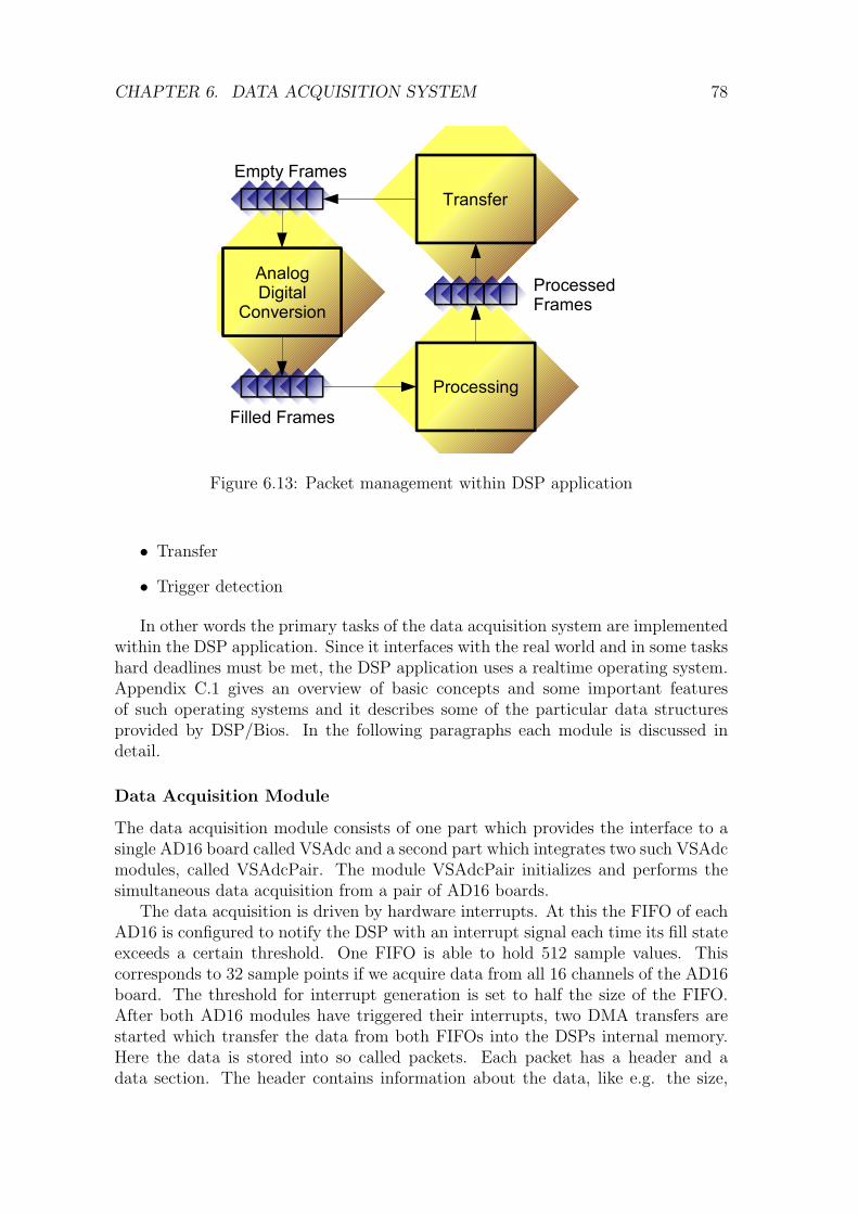
CHAPTER 6. DATA ACQUISITION SYSTEM 78
Figure 6.13: Packet management within DSP application
• Transfer
• Trigger detection
In other words the primary tasks of the data acquisition system are implementedwithin the DSP application. Since it interfaces with the real world and in some taskshard deadlines must be met, the DSP application uses a realtime operating system.Appendix C.1 gives an overview of basic concepts and some important featuresof such operating systems and it describes some of the particular data structuresprovided by DSP/Bios. In the following paragraphs each module is discussed indetail.
Data Acquisition Module
The data acquisition module consists of one part which provides the interface to asingle AD16 board called VSAdc and a second part which integrates two such VSAdcmodules, called VSAdcPair. The module VSAdcPair initializes and performs thesimultaneous data acquisition from a pair of AD16 boards.
The data acquisition is driven by hardware interrupts. At this the FIFO of eachAD16 is configured to notify the DSP with an interrupt signal each time its fill stateexceeds a certain threshold. One FIFO is able to hold 512 sample values. Thiscorresponds to 32 sample points if we acquire data from all 16 channels of the AD16board. The threshold for interrupt generation is set to half the size of the FIFO.After both AD16 modules have triggered their interrupts, two DMA transfers arestarted which transfer the data from both FIFOs into the DSPs internal memory.Here the data is stored into so called packets. Each packet has a header and adata section. The header contains information about the data, like e.g. the size,
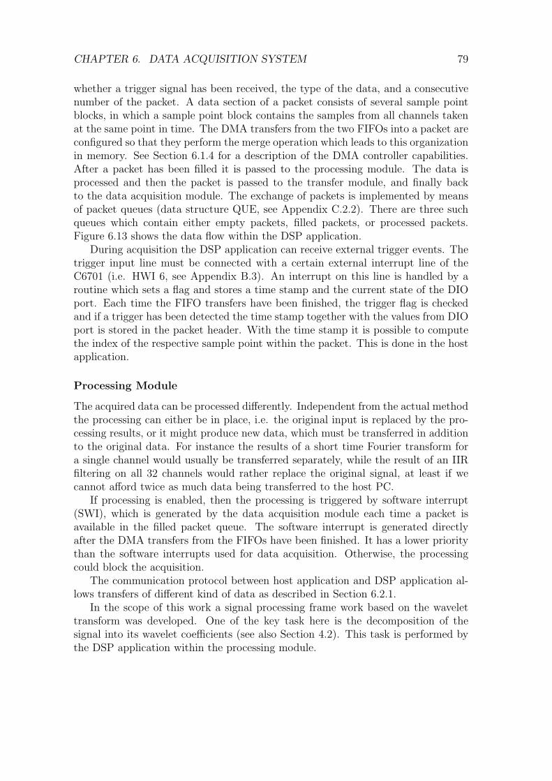
CHAPTER 6. DATA ACQUISITION SYSTEM 79
whether a trigger signal has been received, the type of the data, and a consecutivenumber of the packet. A data section of a packet consists of several sample pointblocks, in which a sample point block contains the samples from all channels takenat the same point in time. The DMA transfers from the two FIFOs into a packet areconfigured so that they perform the merge operation which leads to this organizationin memory. See Section 6.1.4 for a description of the DMA controller capabilities.After a packet has been filled it is passed to the processing module. The data isprocessed and then the packet is passed to the transfer module, and finally backto the data acquisition module. The exchange of packets is implemented by meansof packet queues (data structure QUE, see Appendix C.2.2). There are three suchqueues which contain either empty packets, filled packets, or processed packets.Figure 6.13 shows the data flow within the DSP application.
During acquisition the DSP application can receive external trigger events. Thetrigger input line must be connected with a certain external interrupt line of theC6701 (i.e. HWI 6, see Appendix B.3). An interrupt on this line is handled by aroutine which sets a flag and stores a time stamp and the current state of the DIOport. Each time the FIFO transfers have been finished, the trigger flag is checkedand if a trigger has been detected the time stamp together with the values from DIOport is stored in the packet header. With the time stamp it is possible to computethe index of the respective sample point within the packet. This is done in the hostapplication.
Processing Module
The acquired data can be processed differently. Independent from the actual methodthe processing can either be in place, i.e. the original input is replaced by the pro-cessing results, or it might produce new data, which must be transferred in additionto the original data. For instance the results of a short time Fourier transform fora single channel would usually be transferred separately, while the result of an IIRfiltering on all 32 channels would rather replace the original signal, at least if wecannot afford twice as much data being transferred to the host PC.
If processing is enabled, then the processing is triggered by software interrupt(SWI), which is generated by the data acquisition module each time a packet isavailable in the filled packet queue. The software interrupt is generated directlyafter the DMA transfers from the FIFOs have been finished. It has a lower prioritythan the software interrupts used for data acquisition. Otherwise, the processingcould block the acquisition.
The communication protocol between host application and DSP application al-lows transfers of different kind of data as described in Section 6.2.1.
In the scope of this work a signal processing frame work based on the wavelettransform was developed. One of the key task here is the decomposition of thesignal into its wavelet coefficients (see also Section 4.2). This task is performed bythe DSP application within the processing module.
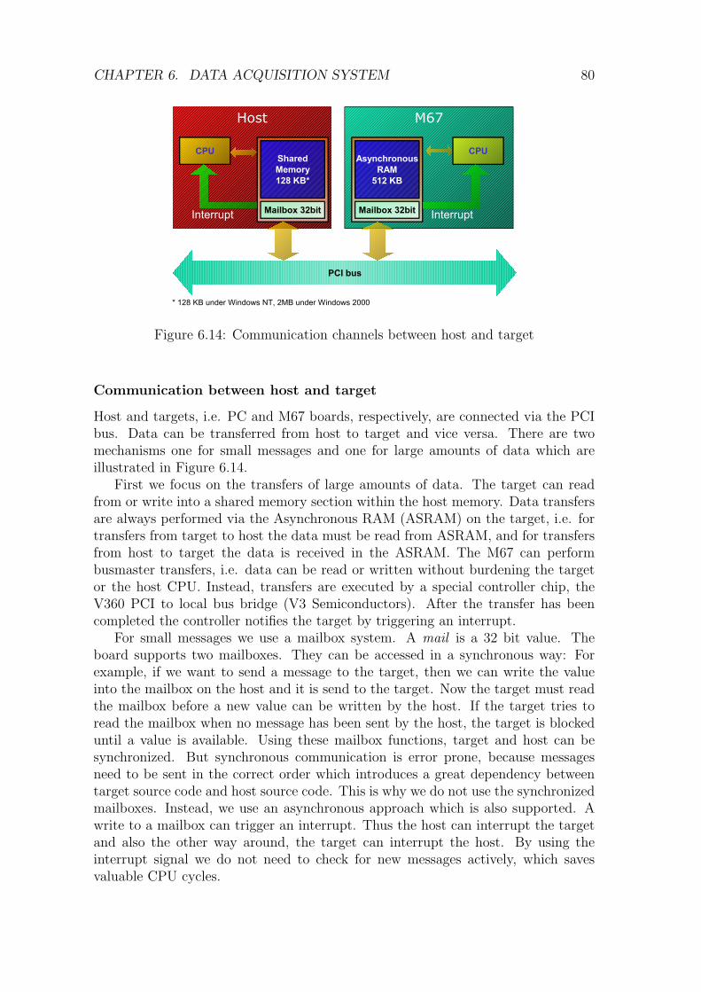
CHAPTER 6. DATA ACQUISITION SYSTEM 80
M67
PCI bus
AsynchronousRAM
512 KB
Mailbox 32bit
Host
Shared Memory128 KB*
Mailbox 32bit
CPU CPU
Interrupt Interrupt
* 128 KB under Windows NT, 2MB under Windows 2000
Figure 6.14: Communication channels between host and target
Communication between host and target
Host and targets, i.e. PC and M67 boards, respectively, are connected via the PCIbus. Data can be transferred from host to target and vice versa. There are twomechanisms one for small messages and one for large amounts of data which areillustrated in Figure 6.14.
First we focus on the transfers of large amounts of data. The target can readfrom or write into a shared memory section within the host memory. Data transfersare always performed via the Asynchronous RAM (ASRAM) on the target, i.e. fortransfers from target to host the data must be read from ASRAM, and for transfersfrom host to target the data is received in the ASRAM. The M67 can performbusmaster transfers, i.e. data can be read or written without burdening the targetor the host CPU. Instead, transfers are executed by a special controller chip, theV360 PCI to local bus bridge (V3 Semiconductors). After the transfer has beencompleted the controller notifies the target by triggering an interrupt.
For small messages we use a mailbox system. A mail is a 32 bit value. Theboard supports two mailboxes. They can be accessed in a synchronous way: Forexample, if we want to send a message to the target, then we can write the valueinto the mailbox on the host and it is send to the target. Now the target must readthe mailbox before a new value can be written by the host. If the target tries toread the mailbox when no message has been sent by the host, the target is blockeduntil a value is available. Using these mailbox functions, target and host can besynchronized. But synchronous communication is error prone, because messagesneed to be sent in the correct order which introduces a great dependency betweentarget source code and host source code. This is why we do not use the synchronizedmailboxes. Instead, we use an asynchronous approach which is also supported. Awrite to a mailbox can trigger an interrupt. Thus the host can interrupt the targetand also the other way around, the target can interrupt the host. By using theinterrupt signal we do not need to check for new messages actively, which savesvaluable CPU cycles.
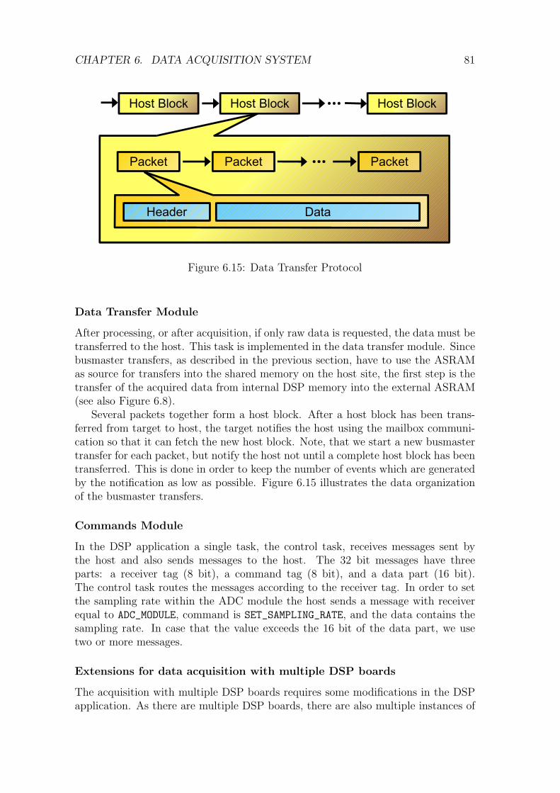
CHAPTER 6. DATA ACQUISITION SYSTEM 81
Host Block
Packet
Header Data
Host Block Host Block
Packet Packet
Figure 6.15: Data Transfer Protocol
Data Transfer Module
After processing, or after acquisition, if only raw data is requested, the data must betransferred to the host. This task is implemented in the data transfer module. Sincebusmaster transfers, as described in the previous section, have to use the ASRAMas source for transfers into the shared memory on the host site, the first step is thetransfer of the acquired data from internal DSP memory into the external ASRAM(see also Figure 6.8).
Several packets together form a host block. After a host block has been trans-ferred from target to host, the target notifies the host using the mailbox communi-cation so that it can fetch the new host block. Note, that we start a new busmastertransfer for each packet, but notify the host not until a complete host block has beentransferred. This is done in order to keep the number of events which are generatedby the notification as low as possible. Figure 6.15 illustrates the data organizationof the busmaster transfers.
Commands Module
In the DSP application a single task, the control task, receives messages sent bythe host and also sends messages to the host. The 32 bit messages have threeparts: a receiver tag (8 bit), a command tag (8 bit), and a data part (16 bit).The control task routes the messages according to the receiver tag. In order to setthe sampling rate within the ADC module the host sends a message with receiverequal to ADC_MODULE, command is SET_SAMPLING_RATE, and the data contains thesampling rate. In case that the value exceeds the 16 bit of the data part, we usetwo or more messages.
Extensions for data acquisition with multiple DSP boards
The acquisition with multiple DSP boards requires some modifications in the DSPapplication. As there are multiple DSP boards, there are also multiple instances of
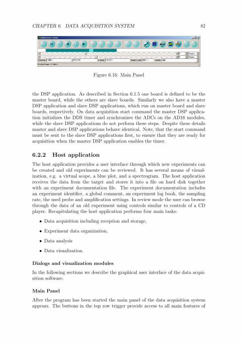
CHAPTER 6. DATA ACQUISITION SYSTEM 82
Figure 6.16: Main Panel
the DSP application. As described in Section 6.1.5 one board is defined to be themaster board, while the others are slave boards. Similarly we also have a masterDSP application and slave DSP applications, which run on master board and slaveboards, respectively. On data acquisition start command the master DSP applica-tion initializes the DDS timer and synchronizes the ADCs on the AD16 modules,while the slave DSP applications do not perform these steps. Despite these detailsmaster and slave DSP applications behave identical. Note, that the start commandmust be sent to the slave DSP applications first, to ensure that they are ready foracquisition when the master DSP application enables the timer.
6.2.2 Host application
The host application provides a user interface through which new experiments canbe created and old experiments can be reviewed. It has several means of visual-ization, e.g. a virtual scope, a blue plot, and a spectrogram. The host applicationreceives the data from the target and stores it into a file on hard disk togetherwith an experiment documentation file. The experiment documentation includesan experiment identifier, a global comment, an experiment log book, the samplingrate, the used probe and amplification settings. In review mode the user can browsethrough the data of an old experiment using controls similar to controls of a CDplayer. Recapitulating the host application performs four main tasks:
• Data acquisition including reception and storage,
• Experiment data organization,
• Data analysis
• Data visualization.
Dialogs and visualization modules
In the following sections we describe the graphical user interface of the data acqui-sition software.
Main Panel
After the program has been started the main panel of the data acquisition systemappears. The buttons in the top row trigger provide access to all main features of

CHAPTER 6. DATA ACQUISITION SYSTEM 83
Open for playback
Close current
Stop playback
Backward play-back
Pause playback
Forward playback
New experiment
Play
Record
Cancel acquisition
Init DAQ HW
Test DAQ HW
Tools
Blue plot
Virtual scope
Spectrogram
Spike plot
Amplifier setup
Quit application
Table 6.5: Activation of visualization modules
the application. They are grouped by functionality (Table 6.5). The first group isactive in replay mode, i.e. if the user reviews already acquired data from disk. Withthe first button (arrow up over rectangle) the user can open such a data file (*.vse or*.h5). The second button (green cross) closes the current file. The next four buttonsare used to start playback in forward and backward mode and to stop or pause theplayback. The playback speed can be modified in the edit field ”Sampling rate”. Thearea under the button row contains several widgets which form the so called browsebar. It is sort of an extended scroll bar and supports the user in browsing throughdatasets which are large in time. Furthermore, it can indicate a selected range withinthe dataset. The rectangular area at the top outlines the settings of the browse barand is called browse bar overview. In its width it represents the full time line of thecurrent data section. In Figure 6.16 the selected range is indicated by dark cyancolored rectangle. The white areas are not in the range. Within the range the lightcyan colored rectangle indicates the part of the data set which is currently storedin the internal data buffer. However, the selected range is independent from theinternal data buffer. Thus, if the selected range starts within or outside this buffer,then the unselected part of the data buffer is indicated by a gray rectangle. Theselection range can be modified by clicking and dragging with right and left mousebutton inside the browse bar overview or with the respective selection edit fields.Inside the rectangle which represents the data buffer, there is another rectangle witha smaller height. This rectangle, which might also be condensed into a vertical line,represents the view buffer, i.e. the section which is currently visualized in the scopeor in the blue plot. The browse bar has two scroll bars. The upper scroll bar movesthe data buffer and the lower scroll bar moves the view buffer within the data buffer.The combo boxes at the right of the scroll bars are used to change the time scale.The number defines a decimation, i.e. the number of values which will be discardedfor each displayed value. Additionally, the decimation mode can be changed. Atthis the application supports nearest neighbor and maximum value.
The New Experiment button (red star) item brings up a dialog which is describedin Section 6.2.2. When a new experiment has been created and the DSP applicationhas been properly initialized, data acquisition may be started by pressing either thePlay (red triangle) or the Rec (red circle) button. If the data acquisition is started
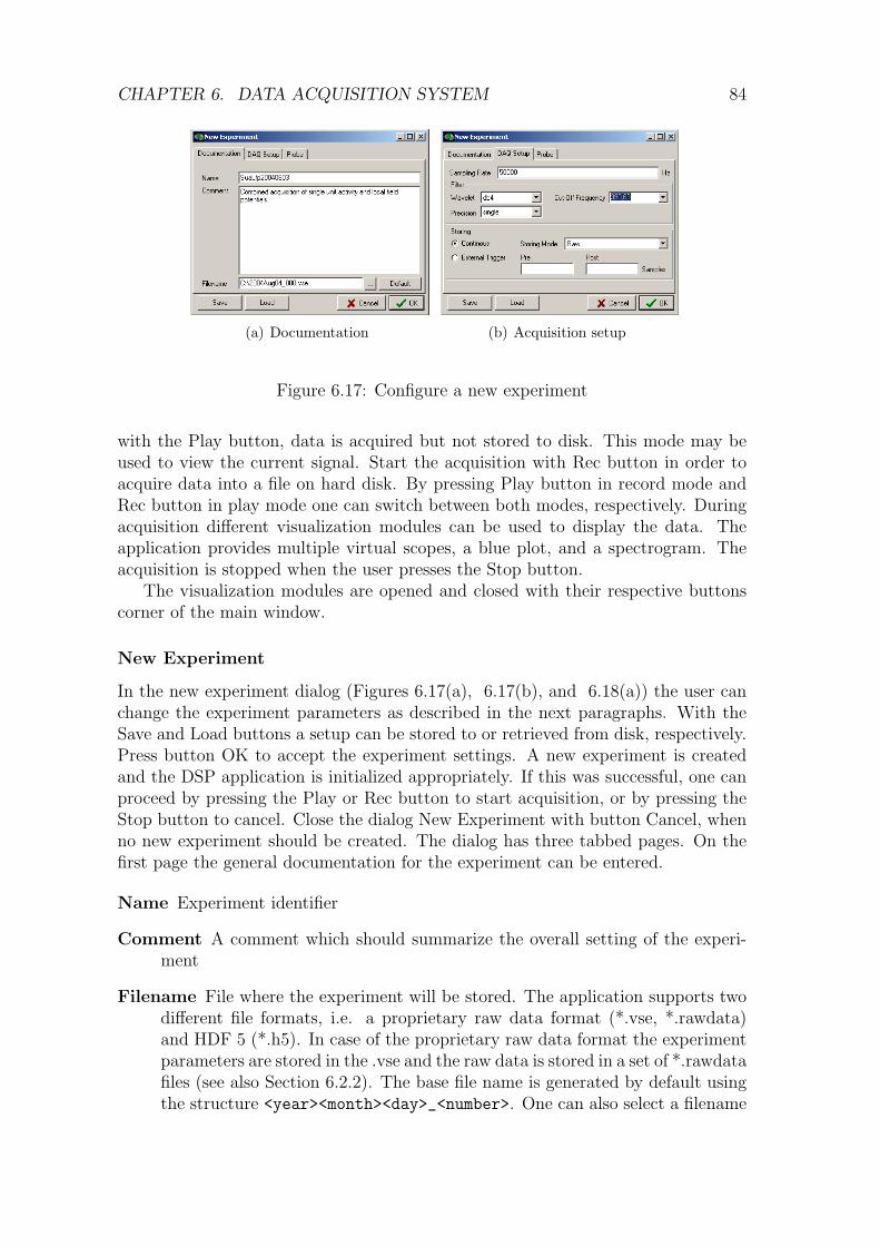
CHAPTER 6. DATA ACQUISITION SYSTEM 84
(a) Documentation (b) Acquisition setup
Figure 6.17: Configure a new experiment
with the Play button, data is acquired but not stored to disk. This mode may beused to view the current signal. Start the acquisition with Rec button in order toacquire data into a file on hard disk. By pressing Play button in record mode andRec button in play mode one can switch between both modes, respectively. Duringacquisition different visualization modules can be used to display the data. Theapplication provides multiple virtual scopes, a blue plot, and a spectrogram. Theacquisition is stopped when the user presses the Stop button.
The visualization modules are opened and closed with their respective buttonscorner of the main window.
New Experiment
In the new experiment dialog (Figures 6.17(a), 6.17(b), and 6.18(a)) the user canchange the experiment parameters as described in the next paragraphs. With theSave and Load buttons a setup can be stored to or retrieved from disk, respectively.Press button OK to accept the experiment settings. A new experiment is createdand the DSP application is initialized appropriately. If this was successful, one canproceed by pressing the Play or Rec button to start acquisition, or by pressing theStop button to cancel. Close the dialog New Experiment with button Cancel, whenno new experiment should be created. The dialog has three tabbed pages. On thefirst page the general documentation for the experiment can be entered.
Name Experiment identifier
Comment A comment which should summarize the overall setting of the experi-ment
Filename File where the experiment will be stored. The application supports twodifferent file formats, i.e. a proprietary raw data format (*.vse, *.rawdata)and HDF 5 (*.h5). In case of the proprietary raw data format the experimentparameters are stored in the .vse and the raw data is stored in a set of *.rawdatafiles (see also Section 6.2.2). The base file name is generated by default usingthe structure <year><month><day>_<number>. One can also select a filename

CHAPTER 6. DATA ACQUISITION SYSTEM 85
in a file select dialog (push button with the three dots), or enter a namemanually. Pressing the button Default generates a default name.
On the tab page DAQSetup the settings for the data acquisition are defined.
Sampling Rate Enter the sampling rate at which the data should be acquired.The rate can range between 5 kHz and 50 kHz.
Filter With these settings the application can be configured to process the acquireddata in a wavelet filter bank. By default, if Wavelet is set to ’none’, thisfiltering is disabled. Otherwise if a certain Wavelet is set, this wavelet isused in the filter bank. With the Precision setting one can select between16 bit integer precision (’int16’) and 32 bit floating (’single’) for the waveletcoefficients. Finally, one can choose the desired cut-off frequency from therespective combo box. Due to the nature of a the filter implementation via andyadic wavelet filter bank, only a certain set of cut-off frequencies is a available(Section 5.1).
Storing The data can be acquired either continuously or based on an externaltrigger. In continuous mode all acquired sample points are stored. They caneither be stored as raw data points, or also as wavelet coefficients. To acquirebased on an external trigger, the number of sample points before and after thetrigger event must be defined. The post trigger sample point count, includesthe sample point which is associated with the trigger event. Thus, the lengthof each sweep is the sum of pre and post triggered samples.
With the Probe tab page a certain probe can be selected which is going to beused in the experiment. New probes can be added in the probe setup dialog whichis opened by button Setup. Each recording site of the probe can be assigned to acertain site group. The groups can have different acquisition settings w.r.t. filterselection and decimation. The table shows all currently specified groups and someof their parameters. In particular a group identifier, a comment, a sampling for thegroup, and a list of recording site assigned to the site group. In the default case allrecording sites are in one group. The button One Group creates this setting andeach time a different probe type is selected, also a single group with all recordingsites of this probe is created. Note, that at this the old setting is lost. With buttonSUA/LFP a setting with two groups one for single unit activity and another forlocal field potentials is prepared. After creation both groups are empty. The usercan select a group with a mouse click into the respective row of the group site tableand then modify the settings in the dialog which is opened by the Configure button(Figure 6.18(b)). In this dialog recordings sites from a list with available sites canbe added to the list of selected recording sites and vice versa. Note, that a sitecan only be assigned to one site group. In the other edit fields group identifier,comment, decimation, and filter type can be defined. Group identifier and commentare arbitrary strings. The decimation is a positive integer or zero. It indicates thenumber of sample points which are discarded for each stored sample point. Thefilter type, which can be none, i.e. disabled, high, or low pass refers to the cut-offfrequency of the filter specified on the DAQ Setup page (Figure 6.17(b)).

CHAPTER 6. DATA ACQUISITION SYSTEM 86
(a) Probe (b) Configure a site group
Figure 6.18: Probe and site group settings
Probe Setup
Within the probe setup dialog (Figure 6.19) new designs of probes can be entered orexisting designs can be edited. The interface assumes that a probe has one or moreshafts, where each shaft is occupied by a certain number of recording sites, whichin turn are vertically oriented on the shaft.
Therefore, the dialog shows three lists: At top the list of probes, in the middle thelist of shafts of the currently selected probe and at the bottom the list of recordingsites of the currently selected shaft. In the table which has the input focus thecurrently selected item is marked by a dashed line around a cell in the row, in bothother tables the selected items are marked by a blue background of one cell in therow. On the left of each table there are three buttons, which create a new item,delete an item, or duplicate an item in the respective table. For example to entera new probe of type E1 one would select a present instance of E1 and duplicate it.It is appended at the end of the list of probes and can be selected. Now one canenter a new comment or number and modify the shaft and site configuration withrespect to the actual probe. The position of the shaft is defined by the position ofits tip. The position of each recording site is specified by the distance to the tip ofthe shaft. Given these informations the spatial relation of two recording sites canbe derived easily. Additionally, the mapping of recording site onto channel numberis defined in this dialog. Note, that channel numbers start at 1.
Amplifier Setup
The amplifier setup dialog is activated by the button with the amplifier symbol(Figure 6.16).
The gain of each site of the current probe can be set in the amplifier setup. Aschema of the probe is drawn in the upper half of the window as shown in Figure 6.20.The gain value can either be selected by using the gain combo box or by clickingonto the legend. The current setting of a gain value is indicated by different colorsfor each site. Each probe has a default gain value setting which can be set pushing

CHAPTER 6. DATA ACQUISITION SYSTEM 87
Figure 6.19: Probe setup dialog
Figure 6.20: Amplifier setup dialog
the Default Gain Settings button. A set of sites can be selected by zooming into theschema of the probe such that only the desired sites are visible. Then the desiredgain can be set for these sites using button Set Gain for Visible Sites.
The dialog is synchronized with the setting at the main amplifier, i.e. manualchanges at the amplifier are visualized by the dialog and vice versa. Manual changingof the gain at the main amplifier can be locked using the button Lock. The buttonindicates the current state by showing the text ”Locked” or ”Unlocked”. The gainsettings are transferred to the amplifier when the Apply button is pressed.
Blueplot
In a blue plot the amplitude of the displayed signals is color coded. The labels onthe x-axis indicate the recording site names. The y-axis is the time line, which canindicate the time stamps of the sample points in terms of an sample point index orin terms of seconds at different scales, i.e. microseconds, milliseconds, or seconds.On the left a color map is displayed. The color mapping can be controlled by mouse

CHAPTER 6. DATA ACQUISITION SYSTEM 88
Figure 6.21: Blueplot
using the sliders in the color bar. They define the range of data values which ismapped onto the colors. If the range has length zero, the sliders define a threshold.It is also possible to change the color map using the combo box at the bottom ofthe color bar. With the button Auto Color Adjust the color mapping is adjusted tothe data currently shown in the blue plot. After this adjustment the median of thecurrent data is mapped on to the center of the color bar. Minimum and maximumare computed based on the mean deviation of the data values from the median. Themapping is symmetric around the median.
The blue plot supports an arbitrary number of traces, at which each trace can beassociated with a recording site or an analyzer result. With the context menu of theblue plot the user can add a trace, remove a trace, and associate a trace with a signal.In Figure 6.21 the context menu is visible. It shows the default configuration fora probe with eight recording site, which is created if the entry Default is selected.The first trace is configured via its context menu. If the user selects the entryRemove, the trace is removed. The entries Sites and Denoiser1 refer to contextmenus which contain the currently available recording sites and denoising resultsfrom Denoiser1. The selection of one entry within these menus sets an associationof the trace with the respective signal. The entry Clear removes all traces from theblue plot. With the entries Load and Save a setup can be retrieved from or storedto a file, respectively.
Spectrogram
The spectrum of a single channel is visualized with the spectrogram. It is basedon the short time Fourier transform which is computed within the host application.The short time Fourier transform is implemented by a fast discrete Fourier transformapplied on a certain time window of the signal. Thus we compute the coefficientsSw,d(k) which depend on the window function w and the time window of signal s(n)selected by offset d:
Sw,d(k) =N−1∑n=0
s(n+ d)w(n)e−j(2π/N)nk
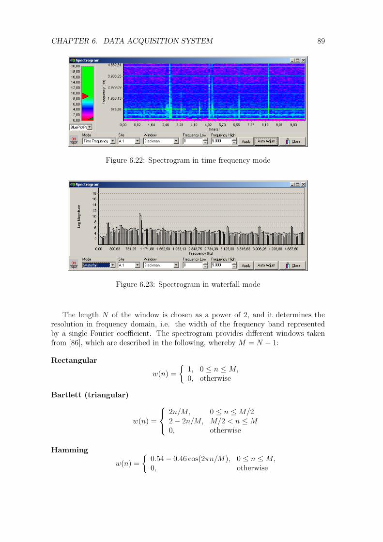
CHAPTER 6. DATA ACQUISITION SYSTEM 89
Figure 6.22: Spectrogram in time frequency mode
Figure 6.23: Spectrogram in waterfall mode
The length N of the window is chosen as a power of 2, and it determines theresolution in frequency domain, i.e. the width of the frequency band representedby a single Fourier coefficient. The spectrogram provides different windows takenfrom [86], which are described in the following, whereby M = N − 1:
Rectangular
w(n) =
1, 0 ≤ n ≤M,0, otherwise
Bartlett (triangular)
w(n) =
2n/M, 0 ≤ n ≤M/22− 2n/M, M/2 < n ≤M0, otherwise
Hamming
w(n) =
0.54− 0.46 cos(2πn/M), 0 ≤ n ≤M,0, otherwise
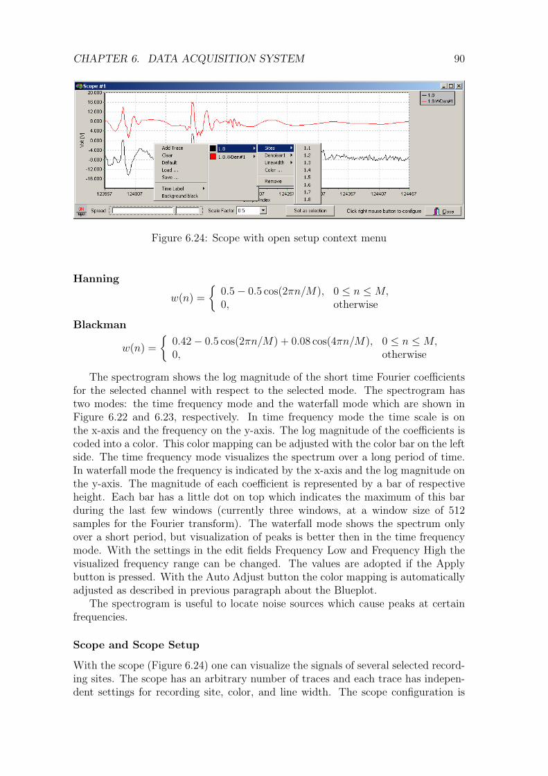
CHAPTER 6. DATA ACQUISITION SYSTEM 90
Figure 6.24: Scope with open setup context menu
Hanning
w(n) =
0.5− 0.5 cos(2πn/M), 0 ≤ n ≤M,0, otherwise
Blackman
w(n) =
0.42− 0.5 cos(2πn/M) + 0.08 cos(4πn/M), 0 ≤ n ≤M,0, otherwise
The spectrogram shows the log magnitude of the short time Fourier coefficientsfor the selected channel with respect to the selected mode. The spectrogram hastwo modes: the time frequency mode and the waterfall mode which are shown inFigure 6.22 and 6.23, respectively. In time frequency mode the time scale is onthe x-axis and the frequency on the y-axis. The log magnitude of the coefficients iscoded into a color. This color mapping can be adjusted with the color bar on the leftside. The time frequency mode visualizes the spectrum over a long period of time.In waterfall mode the frequency is indicated by the x-axis and the log magnitude onthe y-axis. The magnitude of each coefficient is represented by a bar of respectiveheight. Each bar has a little dot on top which indicates the maximum of this barduring the last few windows (currently three windows, at a window size of 512samples for the Fourier transform). The waterfall mode shows the spectrum onlyover a short period, but visualization of peaks is better then in the time frequencymode. With the settings in the edit fields Frequency Low and Frequency High thevisualized frequency range can be changed. The values are adopted if the Applybutton is pressed. With the Auto Adjust button the color mapping is automaticallyadjusted as described in previous paragraph about the Blueplot.
The spectrogram is useful to locate noise sources which cause peaks at certainfrequencies.
Scope and Scope Setup
With the scope (Figure 6.24) one can visualize the signals of several selected record-ing sites. The scope has an arbitrary number of traces and each trace has indepen-dent settings for recording site, color, and line width. The scope configuration is

CHAPTER 6. DATA ACQUISITION SYSTEM 91
Figure 6.25: Menu of tool button
defined with the scope context menu (Figure 6.24) in the same manner as the blueplot (Section 6.2.2). The traces can be spread or overlaid by the track bar at thebottom of the scope. A recording site or result signal is assign to a trace by selectingit from the context menu of the trace. A scope setup can be stored into a file andretrieved by using the Save and Load entries of the context menu, respectively. Thescope is set back into its initial state by the Clear entry. The Default entry createsa configuration where all available recording sites are shown.
The scope has a zoom feature, i.e. the user can select a rectangular region withinthe scope axis, which is in turn enlarged. The region is specified by pressing theleft mouse button at the upper left corner of the rectangle and holding it while themouse is moved to the lower right corner, which is pinned down by releasing theleft mouse button. Note that it is important to specify the upper left corner first,because specifying any other corner first invokes the unzoom function.
The time scale of the scope can be changed with the decimation control of thebrowse bar. A decimation value of k means that only every k-th sample is visualized.In terms of time scale we enlarge the time scale on the x-axis by a factor of k + 1.
Analyzer
The acquired signals can be processed by different analyzers. In general an analyzerhas a set of input signals, i.e. signals from recording sites. The analyzer processesthis data and produces a set of output signals. The user creates a new analyzer byselecting the entry Add Analyzer from the menu of the Tool button (Figure 6.25).The dialog which is shown in Figure 6.26 opens and the user can select the signalswhich shall be processed. Then the method must be selected from the Method combobox. The application supports denoising and filtering. The user may specify a namefor the analyzer and the analyzer is created if the user confirms the configurationwith the OK button. With the Cancel button, the dialog is left without creatinga new analyzer. If no signal was selected, an appropriate message is shown and noanalyzer is created.
Afterwards, on successful creation of an analyzer, it can be configured or removedvia the Tool menu, which contains an entry for each available analyzer (Figure 6.25).The configuration dialogs depend on the actual analyzer and are described in thefollowing paragraphs.
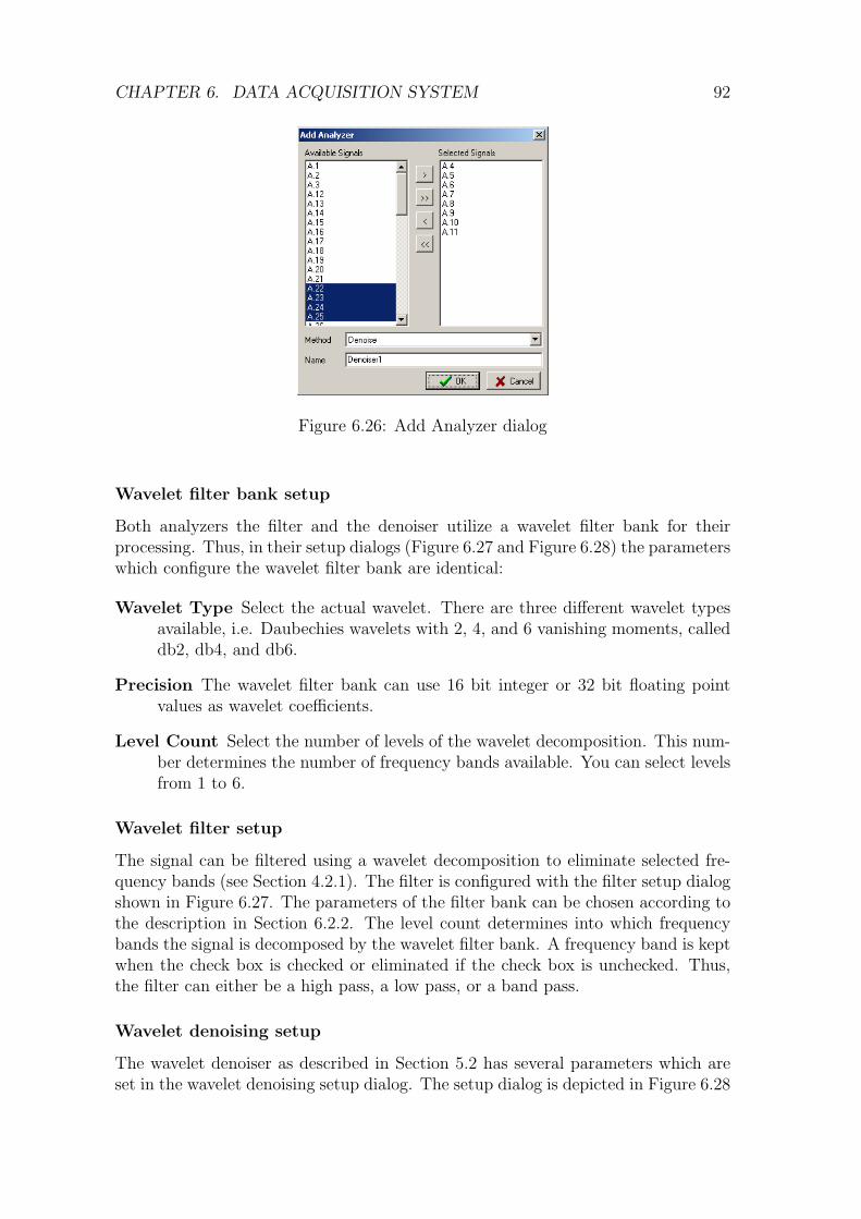
CHAPTER 6. DATA ACQUISITION SYSTEM 92
Figure 6.26: Add Analyzer dialog
Wavelet filter bank setup
Both analyzers the filter and the denoiser utilize a wavelet filter bank for theirprocessing. Thus, in their setup dialogs (Figure 6.27 and Figure 6.28) the parameterswhich configure the wavelet filter bank are identical:
Wavelet Type Select the actual wavelet. There are three different wavelet typesavailable, i.e. Daubechies wavelets with 2, 4, and 6 vanishing moments, calleddb2, db4, and db6.
Precision The wavelet filter bank can use 16 bit integer or 32 bit floating pointvalues as wavelet coefficients.
Level Count Select the number of levels of the wavelet decomposition. This num-ber determines the number of frequency bands available. You can select levelsfrom 1 to 6.
Wavelet filter setup
The signal can be filtered using a wavelet decomposition to eliminate selected fre-quency bands (see Section 4.2.1). The filter is configured with the filter setup dialogshown in Figure 6.27. The parameters of the filter bank can be chosen according tothe description in Section 6.2.2. The level count determines into which frequencybands the signal is decomposed by the wavelet filter bank. A frequency band is keptwhen the check box is checked or eliminated if the check box is unchecked. Thus,the filter can either be a high pass, a low pass, or a band pass.
Wavelet denoising setup
The wavelet denoiser as described in Section 5.2 has several parameters which areset in the wavelet denoising setup dialog. The setup dialog is depicted in Figure 6.28
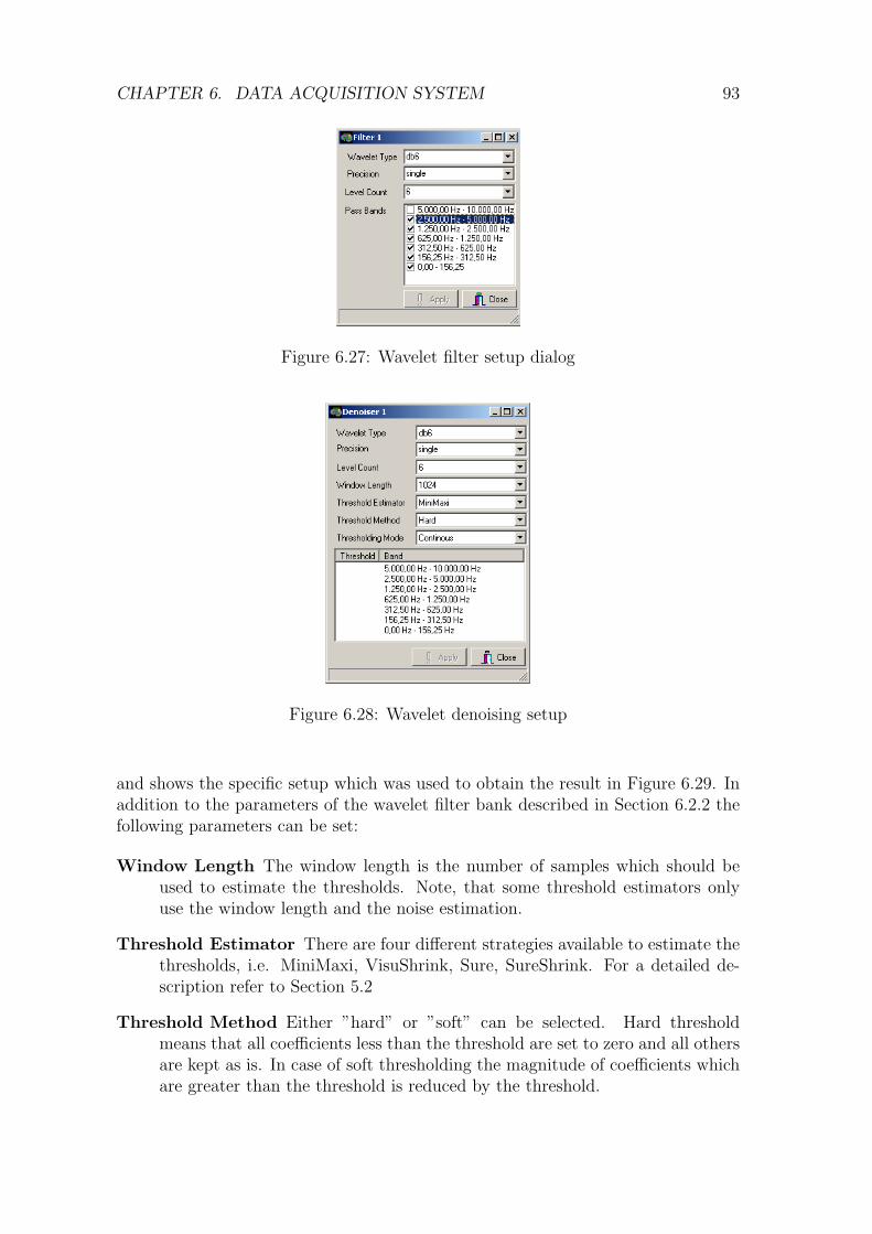
CHAPTER 6. DATA ACQUISITION SYSTEM 93
Figure 6.27: Wavelet filter setup dialog
Figure 6.28: Wavelet denoising setup
and shows the specific setup which was used to obtain the result in Figure 6.29. Inaddition to the parameters of the wavelet filter bank described in Section 6.2.2 thefollowing parameters can be set:
Window Length The window length is the number of samples which should beused to estimate the thresholds. Note, that some threshold estimators onlyuse the window length and the noise estimation.
Threshold Estimator There are four different strategies available to estimate thethresholds, i.e. MiniMaxi, VisuShrink, Sure, SureShrink. For a detailed de-scription refer to Section 5.2
Threshold Method Either ”hard” or ”soft” can be selected. Hard thresholdmeans that all coefficients less than the threshold are set to zero and all othersare kept as is. In case of soft thresholding the magnitude of coefficients whichare greater than the threshold is reduced by the threshold.

CHAPTER 6. DATA ACQUISITION SYSTEM 94
Figure 6.29: Wavelet denoising and Wavelet filtering
Thresholding Mode Choose between continuous or single. In continuous modethe threshold are computed for each window, in single mode the thresholdsare computed for the first window and then used for the subsequent windowswithout change. One can force a recomputation by pressing button ”Recalc”.
Threshold The current thresholds with their respective frequency band are shownand can be changed by the user. The thresholds can range between 0 and32768. However in continuous mode they keep on changing, and thereforemanual change of the thresholds make only sense in single mode. In particularthe threshold for the lowest frequency band can be set to 32768 in order toobtain a high pass filtered denoised signal.
Storage
There are basically two parts that need to be stored, i.e. the experiment parametersand the acquired data. Experiment parameters include e.g. settings from the NewExperiment dialog (Section 6.2.2). The acquired data consists of the values sampledfrom the input signals. During acquisition the user can switch between play andrecord mode. Every time the user switches to record mode, a new data section iscreated. Furthermore, the signals are organized in groups, where each group hasdifferent settings w.r.t to filtering and decimation. Therefore, the acquired data isindexed by two indices, the section index and the site group index.
The data acquisition system supports two file formats. The first file format storesall experiment parameters in a single text file and the acquired data is stored in aset of binary files. Each file corresponds to a certain site group and a certain datasection. The storage format is 16 bit integer in little endian. The following Matlabprogram fragment could be used to load a part of such a file where the number ofsamples and the number of channels must be given.
fid = fopen(’2004Aug05_002.000.001.rawdata’,’r’,’ieee-le’);
s = fread(fid,sample_count*channel_count,’int16=>int16’);
fclose(fid);
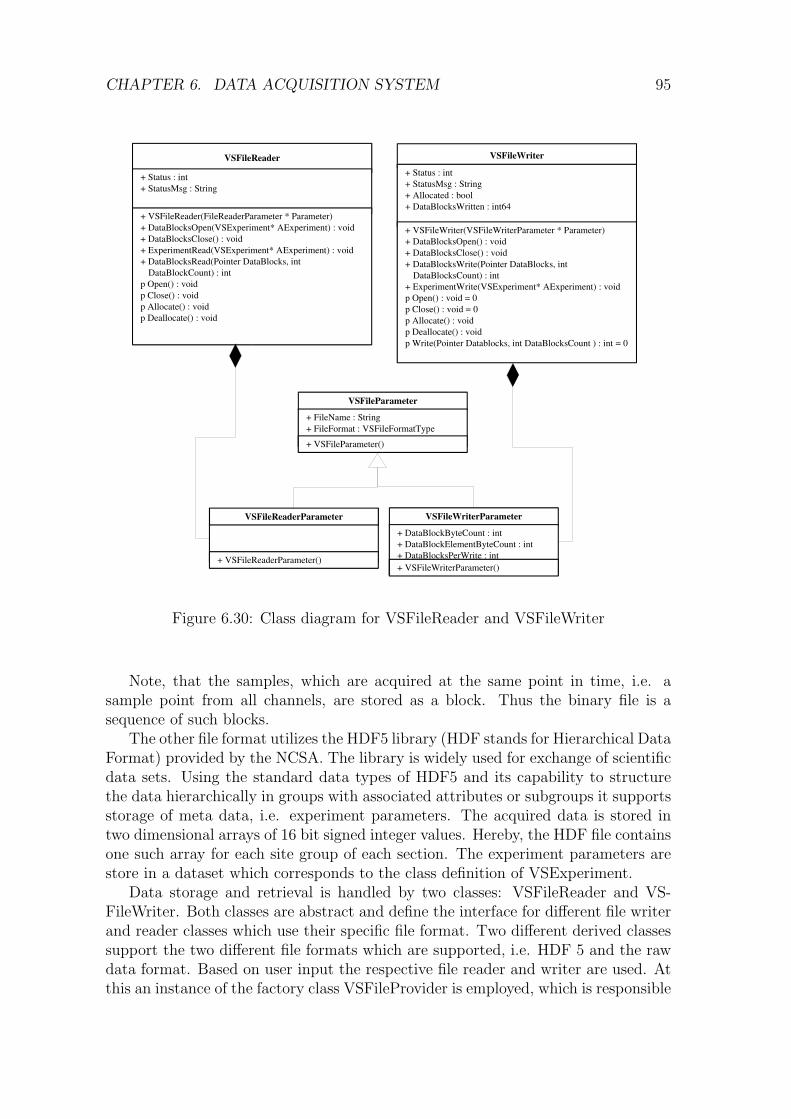
CHAPTER 6. DATA ACQUISITION SYSTEM 95
VSFileReader
+ Status : int+ StatusMsg : String
+ VSFileReader(FileReaderParameter * Parameter) + DataBlocksOpen(VSExperiment* AExperiment) : void+ DataBlocksClose() : void+ ExperimentRead(VSExperiment* AExperiment) : void+ DataBlocksRead(Pointer DataBlocks, int
DataBlockCount) : int p Open() : voidp Close() : voidp Allocate() : voidp Deallocate() : void
VSFileWriter
+ Status : int+ StatusMsg : String+ Allocated : bool+ DataBlocksWritten : int64
+ VSFileWriter(VSFileWriterParameter * Parameter)+ DataBlocksOpen() : void+ DataBlocksClose() : void+ DataBlocksWrite(Pointer DataBlocks, int
DataBlocksCount) : int+ ExperimentWrite(VSExperiment* AExperiment) : voidp Open() : void = 0p Close() : void = 0p Allocate() : voidp Deallocate() : voidp Write(Pointer Datablocks, int DataBlocksCount ) : int = 0
VSFileParameter
+ FileName : String+ FileFormat : VSFileFormatType
+ VSFileParameter()
VSFileReaderParameter
+ VSFileReaderParameter()
VSFileWriterParameter
+ DataBlockByteCount : int+ DataBlockElementByteCount : int+ DataBlocksPerWrite : int+ VSFileWriterParameter()
Figure 6.30: Class diagram for VSFileReader and VSFileWriter
Note, that the samples, which are acquired at the same point in time, i.e. asample point from all channels, are stored as a block. Thus the binary file is asequence of such blocks.
The other file format utilizes the HDF5 library (HDF stands for Hierarchical DataFormat) provided by the NCSA. The library is widely used for exchange of scientificdata sets. Using the standard data types of HDF5 and its capability to structurethe data hierarchically in groups with associated attributes or subgroups it supportsstorage of meta data, i.e. experiment parameters. The acquired data is stored intwo dimensional arrays of 16 bit signed integer values. Hereby, the HDF file containsone such array for each site group of each section. The experiment parameters arestore in a dataset which corresponds to the class definition of VSExperiment.
Data storage and retrieval is handled by two classes: VSFileReader and VS-FileWriter. Both classes are abstract and define the interface for different file writerand reader classes which use their specific file format. Two different derived classessupport the two different file formats which are supported, i.e. HDF 5 and the rawdata format. Based on user input the respective file reader and writer are used. Atthis an instance of the factory class VSFileProvider is employed, which is responsible
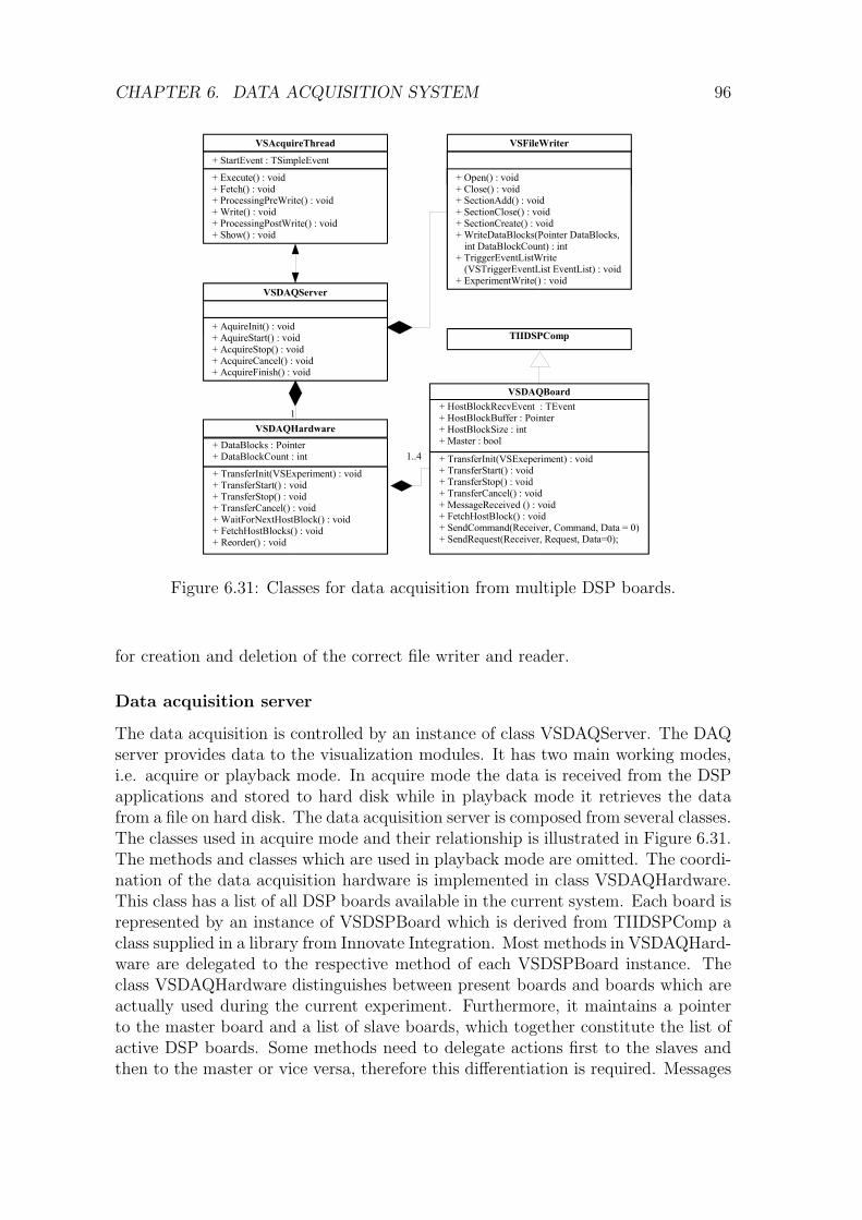
CHAPTER 6. DATA ACQUISITION SYSTEM 96
VSDAQBoard+ HostBlockRecvEvent : TEvent+ HostBlockBuffer : Pointer+ HostBlockSize : int+ Master : bool
+ TransferInit(VSExeperiment) : void+ TransferStart() : void+ TransferStop() : void+ TransferCancel() : void+ MessageReceived () : void + FetchHostBlock() : void+ SendCommand(Receiver, Command, Data = 0) + SendRequest(Receiver, Request, Data=0);
TIIDSPComp
VSDAQHardware+ DataBlocks : Pointer+ DataBlockCount : int
+ TransferInit(VSExperiment) : void+ TransferStart() : void+ TransferStop() : void+ TransferCancel() : void+ WaitForNextHostBlock() : void+ FetchHostBlocks() : void+ Reorder() : void
1..4
VSDAQServer
+ AquireInit() : void+ AquireStart() : void+ AcquireStop() : void+ AcquireCancel() : void+ AcquireFinish() : void
VSAcquireThread
+ StartEvent : TSimpleEvent
+ Execute() : void+ Fetch() : void+ ProcessingPreWrite() : void+ Write() : void+ ProcessingPostWrite() : void+ Show() : void
1
VSFileWriter
+ Open() : void+ Close() : void+ SectionAdd() : void+ SectionClose() : void+ SectionCreate() : void+ WriteDataBlocks(Pointer DataBlocks,
int DataBlockCount) : int + TriggerEventListWrite
(VSTriggerEventList EventList) : void+ ExperimentWrite() : void
Figure 6.31: Classes for data acquisition from multiple DSP boards.
for creation and deletion of the correct file writer and reader.
Data acquisition server
The data acquisition is controlled by an instance of class VSDAQServer. The DAQserver provides data to the visualization modules. It has two main working modes,i.e. acquire or playback mode. In acquire mode the data is received from the DSPapplications and stored to hard disk while in playback mode it retrieves the datafrom a file on hard disk. The data acquisition server is composed from several classes.The classes used in acquire mode and their relationship is illustrated in Figure 6.31.The methods and classes which are used in playback mode are omitted. The coordi-nation of the data acquisition hardware is implemented in class VSDAQHardware.This class has a list of all DSP boards available in the current system. Each board isrepresented by an instance of VSDSPBoard which is derived from TIIDSPComp aclass supplied in a library from Innovate Integration. Most methods in VSDAQHard-ware are delegated to the respective method of each VSDSPBoard instance. Theclass VSDAQHardware distinguishes between present boards and boards which areactually used during the current experiment. Furthermore, it maintains a pointerto the master board and a list of slave boards, which together constitute the list ofactive DSP boards. Some methods need to delegate actions first to the slaves andthen to the master or vice versa, therefore this differentiation is required. Messages
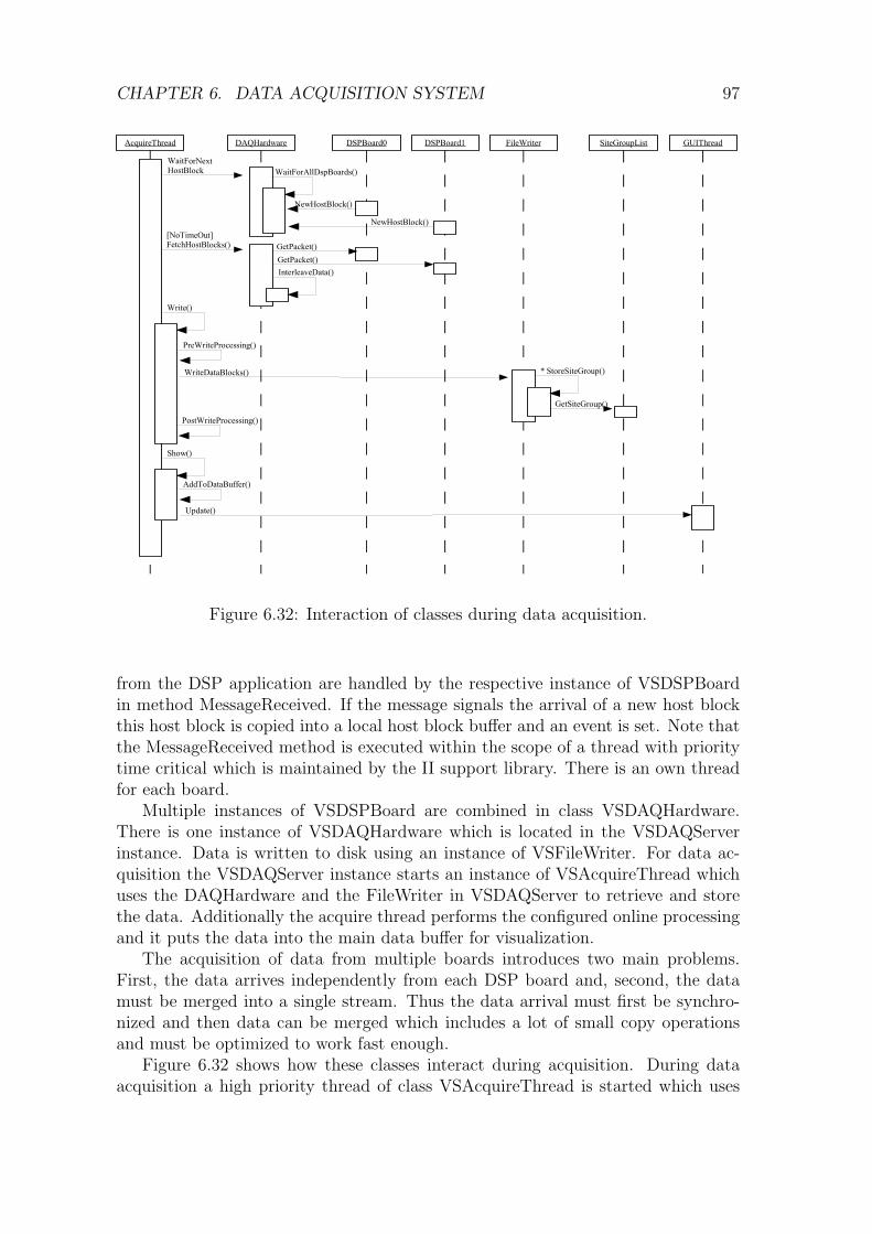
CHAPTER 6. DATA ACQUISITION SYSTEM 97
GUIThreadSiteGroupListFileWriterDSPBoard1DSPBoard0DAQHardwareAcquireThread
WaitForNextHostBlock WaitForAllDspBoards()
NewHostBlock()
NewHostBlock()[NoTimeOut]FetchHostBlocks() GetPacket()
GetPacket()InterleaveData()
Write()
PreWriteProcessing()
PostWriteProcessing()
WriteDataBlocks() * StoreSiteGroup()
GetSiteGroup()
Show()
AddToDataBuffer()
Update()
Figure 6.32: Interaction of classes during data acquisition.
from the DSP application are handled by the respective instance of VSDSPBoardin method MessageReceived. If the message signals the arrival of a new host blockthis host block is copied into a local host block buffer and an event is set. Note thatthe MessageReceived method is executed within the scope of a thread with prioritytime critical which is maintained by the II support library. There is an own threadfor each board.
Multiple instances of VSDSPBoard are combined in class VSDAQHardware.There is one instance of VSDAQHardware which is located in the VSDAQServerinstance. Data is written to disk using an instance of VSFileWriter. For data ac-quisition the VSDAQServer instance starts an instance of VSAcquireThread whichuses the DAQHardware and the FileWriter in VSDAQServer to retrieve and storethe data. Additionally the acquire thread performs the configured online processingand it puts the data into the main data buffer for visualization.
The acquisition of data from multiple boards introduces two main problems.First, the data arrives independently from each DSP board and, second, the datamust be merged into a single stream. Thus the data arrival must first be synchro-nized and then data can be merged which includes a lot of small copy operationsand must be optimized to work fast enough.
Figure 6.32 shows how these classes interact during acquisition. During dataacquisition a high priority thread of class VSAcquireThread is started which uses

CHAPTER 6. DATA ACQUISITION SYSTEM 98
StoringMode ProcessingPreWrite ProcessingPostWriteRaw nothing Wavelet filter bankRawFiltered Wavelet filter bank nothingWavelet Coefficients Wavelet decomposition
and coefficient delayCoefficient processingand wavelet reconstruc-tion.
Table 6.6: Post- and pre-write processing
the method WaitForNextHostBlock in class VSDAQHardware in order to wait untileach DSP application has sent the host block. Data arrival is indicated by a cer-tain message from the DSP application. On message reception the MessageReceivemethod of the respective VSDSPBoard instance is called in the scope of a threadrunning within the DSP board driver with high priority. This methods sets theHostBlockRecvEvent which indicates that a new host block has arrived from therespective DSP application. If any board did not send new data then a time outoccurs and the acquire thread terminates. However, if all boards deliver their hostblock the acquire thread fetches the data from all DSP boards and merges it intoa single stream within method FetchHostBlocks. The merge operation is shown inFigure 6.33 and the reordering in Figure 6.34. The data blocks are then processedin the ProcessingPreWrite method, then written to disk, and again processed inthe ProcessingPostWrite method. The actual processing performed in both meth-ods depends on the storing mode and Table 6.6 shows the different cases. Data iswritten to disk with the FileWriter in method WriteDataBlocks. The SiteGroupListin FileWriterParameter contains the parameters which determine subsampling andfilter settings for the acquired data.
Data reception
This section addresses the merging and reordering of raw data from multiple DSPboards illustrated in Figure 6.33 and Figure 6.34. As described in Section 6.2.1 thedata transfers is organized in host blocks and packets. The data arrives at the hostPC in the shared memory area of each DSP board. A host block is divided intopackets, and each packet has a header and a data part. In Figure 6.33 the header isshortly represented by its packet id, but contains some additional information. Thepacket id is used to detect packet losses. If the host was for some reason not able tofetch the data in time, packets might have been overwritten by the DSP application.In this case the sequence of packet ids will not be steadily increasing, and there willbe a detectable gap. The data part of the packets contains the acquired valuesorganized as shown by the schema at the bottom of Figure 6.33. For each point inthe time the sample values from all 32 channels are stored sequentially in memory.The acquisition DSP board acquires the 32 channels at 16 bit. Therefore one samplepoint has 64 bytes. The data part of each packet contains N sample points. Firstwe merge the packets into a data buffer so that the the N sample points from threeDSPs form a block in memory. Then this block is reordered such that each sample
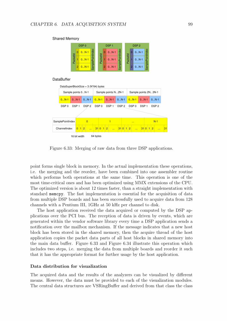
CHAPTER 6. DATA ACQUISITION SYSTEM 99
SamplePointIndex
ChannelIndex
1 ... N10
0 311 2 ... 0 311 2 ... 0 311 2 ...0 311 2 ...
16 bit width 64 bytes
0...N1 0...N1 0...N1 0...N1 0...N1 0...N1 0...N1 0...N1 0...N1
Sample points 0...N1 Sample points N...2N1 Sample points 2N...3N1
DataSuperBlockSize = 3 (N*64) bytes
DSP 0 DSP 1 DSP 2 DSP 0 DSP 1 DSP 2 DSP 0 DSP 1 DSP 2
Shared Memory
Pac
ketId
Sam
pleP
oint
Inde
x
DSP 0
0...N11
0...N12
0...N10
Pac
ketId
Sam
pleP
oint
Inde
x
0...N12
0...N10
0...N11
DSP 2
Pac
ketId
Sam
pleP
oint
Inde
x
0...N12
0...N11
0...N10
DSP 1
DataBuffer
Figure 6.33: Merging of raw data from three DSP applications.
point forms single block in memory. In the actual implementation these operations,i.e. the merging and the reorder, have been combined into one assembler routinewhich performs both operations at the same time. This operation is one of themost time-critical ones and has been optimized using MMX extensions of the CPU.The optimized version is about 12 times faster, than a straight implementation withstandard memcpy. The fast implementation is essential for the acquisition of datafrom multiple DSP boards and has been successfully used to acquire data from 128channels with a Pentium III, 1GHz at 50 kHz per channel to disk.
The host application received the data acquired or computed by the DSP ap-plications over the PCI bus. The reception of data is driven by events, which aregenerated within the vendor software library every time a DSP application sends anotification over the mailbox mechanism. If the message indicates that a new hostblock has been stored in the shared memory, then the acquire thread of the hostapplication copies the packet data parts of all host blocks in shared memory intothe main data buffer. Figure 6.33 and Figure 6.34 illustrate this operation whichincludes two steps, i.e. merging the data from multiple boards and reorder it suchthat it has the appropriate format for further usage by the host application.
Data distribution for visualization
The acquired data and the results of the analyzers can be visualized by differentmeans. However, the data must be provided to each of the visualization modules.The central data structures are VSRingBuffer and derived from that class the class

CHAPTER 6. DATA ACQUISITION SYSTEM 100
SamplePointIndex N1...210 N1...210 N1...210
N1 N1 N1.........
SamplePointIndex 000 111 222
DSP 0 DSP 1 DSP 2
Figure 6.34: Reorder of acquired data after copy from shared memory, which isnecessary if acquisition uses multiple DSP boards.
VSDataBuffer. The class VSRingBuffer implements a ring buffer. Data can beadded or removed at head and at the tail of this particular ring buffer, which is usedduring forward and backward playback from disk. Counters and indices of VSRing-Buffer are byte oriented. VSDataBuffer divides the actual buffer into data blockswith all of them having the same size at construction of an instance. Through theclass each data block can be addressed by a global 64 bit index. The class providesa mechanism to keep track of already read data and newly added data. In Fig-ure 6.35 a class diagram illustrates the features of VSDataBuffer and VSRingbuffer.The data is distributed to different visualisation modules by class VSDataBuffer-View which is associated with VSModule. Details of both classes are shown in Fig-ure 6.36. The class VSModule holds views for all data buffers, and a reference to thecurrent experiment parameters. With method Update of VSModule the data bufferviews are moved to the given position ViewIndexHead. This method is for examplecalled after the view position has been changed in the browse bar. With the classVSDataBufferView one can extract a segment of data blocks from the associatedVSDataBuffer instance. Hereby, it supports decimation of data in two modes, i.e.nearest neighbor and maximum over the decimation interval. VSModule provides aninterface for the main dialog to all visualization modules and visualization modulescan execute methods of the main dialog through the VSModule class. Thus, eachvisualisation dialog has an own instance of VSModule. On the other hand the maindialog maintains a list of VSModule instances which is used to triggered differentactions on all modules. If for instance the visualization modules need to be updatedthe method the main dialog calls the Update method of each VSModule instance inthe list. The same mechanism is used for Allocate, Deallocate, and Reset.
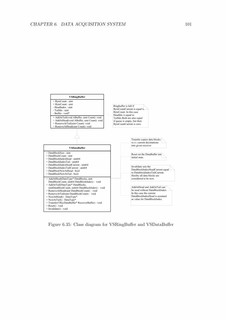
CHAPTER 6. DATA ACQUISITION SYSTEM 101
VSDataBuffer
+ DataBlockSize : uint+ DataBlockCount : uint+ DataBlockIndexHead : uint64+ DataBlockIndexTail : uint64+ DataBlockIndexHeadCurrent : uint64+ DataBlockIndexTailCurrent : uint64+ DataBlockNewAtHead : bool+ DataBlockNewAtTail : bool
+ Decimation : uint+ AddAtHead(DataType* DataBlocks, uint DataBlockCount, uint64 DataBlockIndex) : void
+ AddAtTail(DataType* DataBlocks, uintDataBlockCount, uint64 DataBlockIndex) : void
+ RemoveAtHead(uint DataBlockCount) : void+ RemoveAtTail(uint DataBlockCount) : void+ NextAtHead() : DataType*+ NextAtTail() : DataType*+ Transfer(TRecDataBuffer* ReceiverBuffer) : void+ Reset() : void+ Invalidate() : void
VSRingBuffer+ ByteCount : uint+ ByteCount : uint- HeadIndex : uint- TailIdx : uint- Buffer : void*+ AddAtTail(void ABuffer, uint Count): void+ AddAtHead(void ABuffer, uint Count): void+ RemoveAtTail(uint Count): void+ RemoveAtHead(uint Count): void
Ringbuffer is full if ByteCountCurrent is equal to ByteCount. In this case HeadIdx is equal to TailIdx.Both are also equal if queue is empty, but then ByteCountCurrent is zero.
Transfer copies data blocks w.r.t. current decimations into given receiver
Reset set the DataBuffer into initial state.
Invalidate sets the DataBlockIndexHeadCurrent equal to DatablockIndexTailCurrent. Hereby all data blocks are considered to be new.
AddAtHead and AddAtTail can be used without DataBlockIndex. In this case the current DataBlockIndexHead is assumed as value for DataBlockIndex.
Figure 6.35: Class diagram for VSRingBuffer and VSDataBuffer

CHAPTER 6. DATA ACQUISITION SYSTEM 102
VSDataBuffer
DataBuffer
A DataBufferView updates it self from the data buffer so that the selected data is in the view.
Provide an unified interface for all modules that need data. This can be extended for a more sophisticated data selection, i.e. select only particular channels.
Events that are used to notify the module about initialization, new data, or need for reset.
Enable or disable a module, i.e. DataBufferView is not updated.
DataBufferView ResultBufferViewList
VSModule
+ Experiment : VSExperiment+ OnAllocate : TNotifyEvent+ OnDeallocate : TNotifyEvent+ OnReset : TNotifyEvent+ OnUpdate: TNotifyEvent+ Enabled : bool
+ Update(int64 ViewIndexHead, int64 Decimation, VSDecimationModeType DecimationMode) : void
+ UpdateAtHead(int64 Decimation, VSDecimationModeType DecimationMode) : void
*1
VSDataBufferView
+ Decimation : uint+ IndexHead : int64+ IndexTail : int64
+ Move(int64 ViewIndexHead, int64 Decimation, VSDecimationMode DecimationMode) : void
+ Reset() : void
Figure 6.36: Classes for data distribution
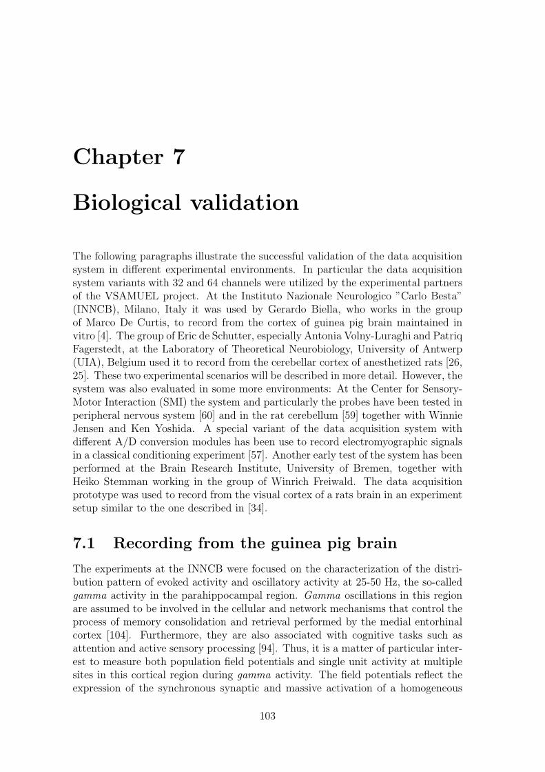
Chapter 7
Biological validation
The following paragraphs illustrate the successful validation of the data acquisitionsystem in different experimental environments. In particular the data acquisitionsystem variants with 32 and 64 channels were utilized by the experimental partnersof the VSAMUEL project. At the Instituto Nazionale Neurologico ”Carlo Besta”(INNCB), Milano, Italy it was used by Gerardo Biella, who works in the groupof Marco De Curtis, to record from the cortex of guinea pig brain maintained invitro [4]. The group of Eric de Schutter, especially Antonia Volny-Luraghi and PatriqFagerstedt, at the Laboratory of Theoretical Neurobiology, University of Antwerp(UIA), Belgium used it to record from the cerebellar cortex of anesthetized rats [26,25]. These two experimental scenarios will be described in more detail. However, thesystem was also evaluated in some more environments: At the Center for Sensory-Motor Interaction (SMI) the system and particularly the probes have been tested inperipheral nervous system [60] and in the rat cerebellum [59] together with WinnieJensen and Ken Yoshida. A special variant of the data acquisition system withdifferent A/D conversion modules has been use to record electromyographic signalsin a classical conditioning experiment [57]. Another early test of the system has beenperformed at the Brain Research Institute, University of Bremen, together withHeiko Stemman working in the group of Winrich Freiwald. The data acquisitionprototype was used to record from the visual cortex of a rats brain in an experimentsetup similar to the one described in [34].
7.1 Recording from the guinea pig brain
The experiments at the INNCB were focused on the characterization of the distri-bution pattern of evoked activity and oscillatory activity at 25-50 Hz, the so-calledgamma activity in the parahippocampal region. Gamma oscillations in this regionare assumed to be involved in the cellular and network mechanisms that control theprocess of memory consolidation and retrieval performed by the medial entorhinalcortex [104]. Furthermore, they are also associated with cognitive tasks such asattention and active sensory processing [94]. Thus, it is a matter of particular inter-est to measure both population field potentials and single unit activity at multiplesites in this cortical region during gamma activity. The field potentials reflect theexpression of the synchronous synaptic and massive activation of a homogeneous
103
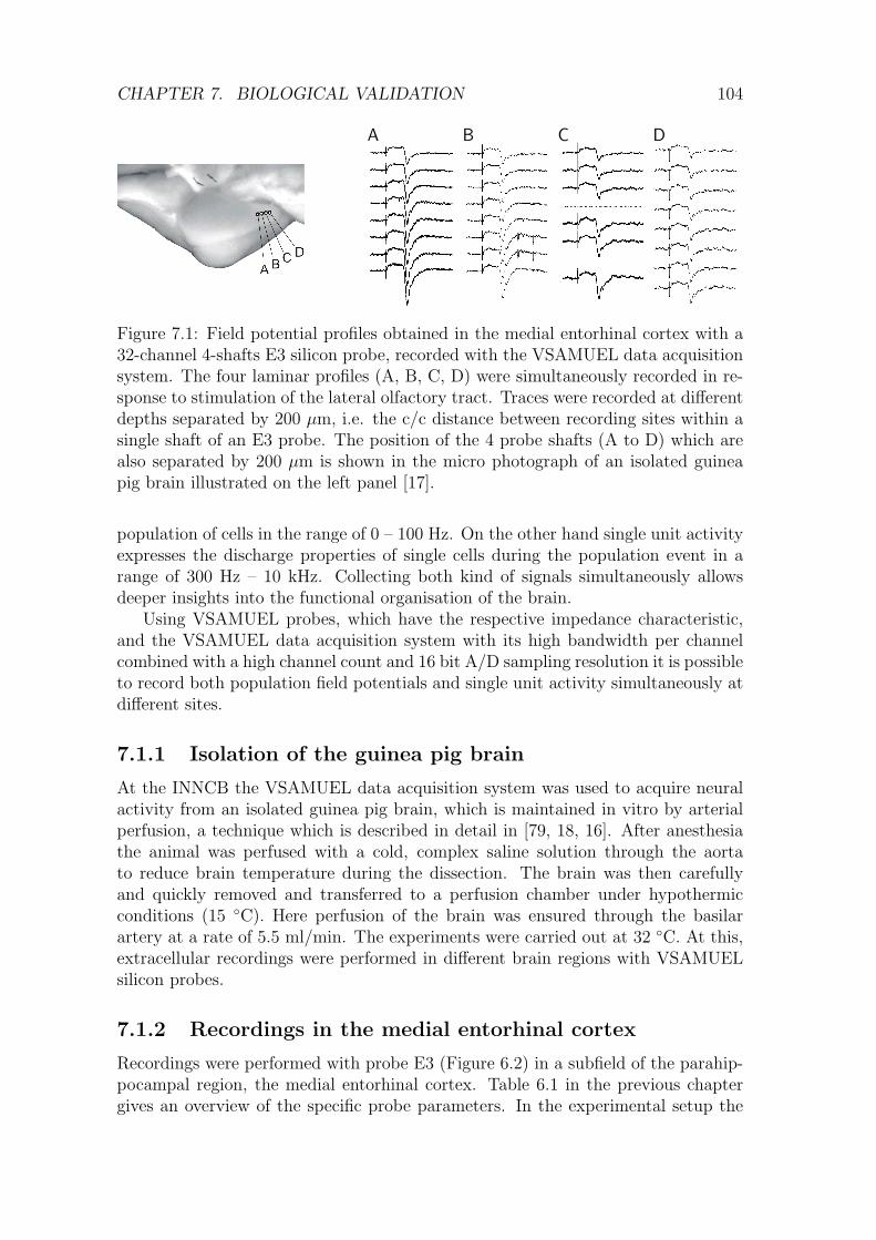
CHAPTER 7. BIOLOGICAL VALIDATION 104
A B C D
Figure 7.1: Field potential profiles obtained in the medial entorhinal cortex with a32-channel 4-shafts E3 silicon probe, recorded with the VSAMUEL data acquisitionsystem. The four laminar profiles (A, B, C, D) were simultaneously recorded in re-sponse to stimulation of the lateral olfactory tract. Traces were recorded at differentdepths separated by 200 µm, i.e. the c/c distance between recording sites within asingle shaft of an E3 probe. The position of the 4 probe shafts (A to D) which arealso separated by 200 µm is shown in the micro photograph of an isolated guineapig brain illustrated on the left panel [17].
population of cells in the range of 0 – 100 Hz. On the other hand single unit activityexpresses the discharge properties of single cells during the population event in arange of 300 Hz – 10 kHz. Collecting both kind of signals simultaneously allowsdeeper insights into the functional organisation of the brain.
Using VSAMUEL probes, which have the respective impedance characteristic,and the VSAMUEL data acquisition system with its high bandwidth per channelcombined with a high channel count and 16 bit A/D sampling resolution it is possibleto record both population field potentials and single unit activity simultaneously atdifferent sites.
7.1.1 Isolation of the guinea pig brain
At the INNCB the VSAMUEL data acquisition system was used to acquire neuralactivity from an isolated guinea pig brain, which is maintained in vitro by arterialperfusion, a technique which is described in detail in [79, 18, 16]. After anesthesiathe animal was perfused with a cold, complex saline solution through the aortato reduce brain temperature during the dissection. The brain was then carefullyand quickly removed and transferred to a perfusion chamber under hypothermicconditions (15 C). Here perfusion of the brain was ensured through the basilarartery at a rate of 5.5 ml/min. The experiments were carried out at 32 C. At this,extracellular recordings were performed in different brain regions with VSAMUELsilicon probes.
7.1.2 Recordings in the medial entorhinal cortex
Recordings were performed with probe E3 (Figure 6.2) in a subfield of the parahip-pocampal region, the medial entorhinal cortex. Table 6.1 in the previous chaptergives an overview of the specific probe parameters. In the experimental setup the

CHAPTER 7. BIOLOGICAL VALIDATION 105
A
B
C
D
Figure 7.2: Simultaneous recording from 4 sites (A to D, separated by 0.5 mm) inthe medial entorhinal cortex with an ACREO-E3 silicon probe after induction of fastgamma oscillations by arterial perfusion of the isolated guinea pig brain preparationwith 50 µM carbachol. Each shaft featured 8 recording sites separated by 200 µm.Leads 4 and 7 on shaft C were not connected. [17]
signal was amplified by a factor of 1000 and filtered with an analog band pass filterwith cut off frequencies at 0.1 Hz and 5 kHz and acquired at 20 kHz sampling ratefor offline analysis.
Figure 7.1 shows typical responses in olfactory/limbic cortices evoked by bipolarstimulation of the lateral olfactory tract [2]. Each column illustrates the potentialsrecorded at 8 different depths. The order of the signals from top to bottom corre-sponds to an anatomical order from surface to depth. Recording sites within theshafts are separated by 0.2 mm from each other as well as the shafts. Note that thetwo dotted lines in the illustration indicate two recording leads on shaft C, whichwere not correctly connected on the used E3 probe.
Figure 7.2 illustrates a typical recording from 4 sites after induction of fastgamma oscillations obtained with E3 probe. The gamma activity at 25–40 Hz inthe medial entorhinal cortex has been invoked by pharmacological stimulation withthe muscarine receptor agonist carbachol (50 µM applied by arterial perfusion) [100,19, 20]. The simultaneous recording from 4 different shafts separated by 0.2 mmand at the same time also at 8 different depths allowed to verify the depth reversalof activity, which can be observed across the cortical depth for locally generatedpotentials [3]. Therefore the measured depth reversal of the potential allows todistinguish whether the activity is generated by the cortex or by a far field volumeconducted from a distant source [17, 43].
Figure 7.3 shows an example where also single unit activity has been recorded inthe same experimental setup illustrated with Figure 7.2 and Figure 7.1. The filtersettings (high-pass filter at 0.1 Hz and low-pass filter at 5 kHz) allowed to recordslow events as well as fast activities generated by single cells. The respective spikes

CHAPTER 7. BIOLOGICAL VALIDATION 106
Figure 7.3: Single unit recordings performed with a M2 probe. The traces from 8channels in a single probe shaft are illustrated in B. The unitary activities of twocells outlined by the box in B are illustrated at fast time resolution in the upperright panel C proving the wide band acquisition purposes of the VSAMUEL dataacquisition system. [17]
from two different cells are displayed in the close up in panel C, marked with anasterisk and a filled circle, respectively [43]. Actually, this proves the wide bandacquisition purposes of the VSAMUEL data acquisition system.
The experiment which is illustrated with Figure 7.4 is used to investigate the ver-tical organization of the cortex, i.e. interaction between layers within a restrictedpatch of cortex. For the vertical study it is crucial to explore at the same timethe entire depth of the cortex (1.2-1.4 mm). To validate the use of the 32 channelVSAMUEL data acquisition system laminar profiles were performed in the entorhi-nal cortex and dentate gyrus of the hippocampus following electrical stimulationof the lateral olfactory tract (LOT), which is indicated by an arrow at the leftof the field potential profile in Figure 7.4. The stimulation artifact is followedby the response measured in the dentate gyrus (DG) of the hippocampus. PanelA shows superimposed traces which represent the average of 7 responses simulta-neously recorded at 20 adjacent recording sites, selected out of the 32 availablechannels. Below in panel B the traces are separated with respect to the recordingdepth. The photograph of the right shows the electrode track reconstructed on ahistological sections cut after fixing the brain with a mixed aldehydes solution. Fi-nally, panel C shows the contour plot of the sink/source distribution obtained byperforming current source density analysis on the laminar potential profile. Sinksand sources are illustrated by continuous and dotted lines, respectively. The currentsource density is calculated as the discrete second-order differentiation of the fieldpotential function ψ(z, t) along the depth z:
CSD(z, t) = σ2ψ(z, t)− ψ(z −N∆z, t)− ψ(z +N∆z, t)
(N∆z)2(7.1)
where ∆z is the distance between the recording sites and t is the time variable.Conductivity σ is assumed to be constant over depth.
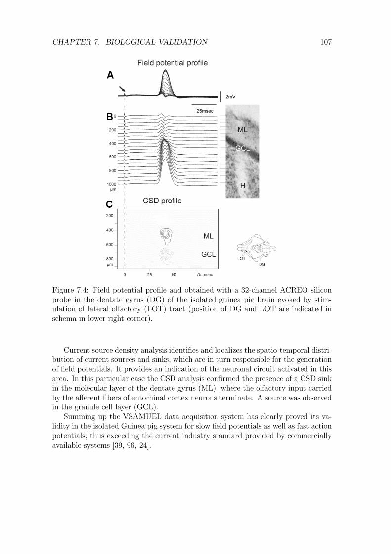
CHAPTER 7. BIOLOGICAL VALIDATION 107
Figure 7.4: Field potential profile and obtained with a 32-channel ACREO siliconprobe in the dentate gyrus (DG) of the isolated guinea pig brain evoked by stim-ulation of lateral olfactory (LOT) tract (position of DG and LOT are indicated inschema in lower right corner).
Current source density analysis identifies and localizes the spatio-temporal distri-bution of current sources and sinks, which are in turn responsible for the generationof field potentials. It provides an indication of the neuronal circuit activated in thisarea. In this particular case the CSD analysis confirmed the presence of a CSD sinkin the molecular layer of the dentate gyrus (ML), where the olfactory input carriedby the afferent fibers of entorhinal cortex neurons terminate. A source was observedin the granule cell layer (GCL).
Summing up the VSAMUEL data acquisition system has clearly proved its va-lidity in the isolated Guinea pig system for slow field potentials as well as fast actionpotentials, thus exceeding the current industry standard provided by commerciallyavailable systems [39, 96, 24].

CHAPTER 7. BIOLOGICAL VALIDATION 108
Figure 7.5: Receptive fields in the Crus II and PML (paramedian lobule) regionsof the cerebellar cortex related to tactile stimuli. The insertion positions of theVSAMUEL probes are indicated by the elongated red areas.
Figure 7.6: Five multi unit recordings representing spiking cerebellar neurons inresponse to tactile stimulus to the upper lip of the face recorded with an E1 probe.The names on the left side indicate the recording site by shaft name and site number(numbering start at the tip of the shaft)
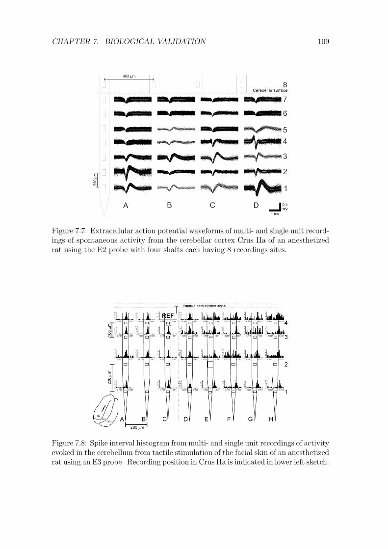
CHAPTER 7. BIOLOGICAL VALIDATION 109
Figure 7.7: Extracellular action potential waveforms of multi- and single unit record-ings of spontaneous activity from the cerebellar cortex Crus IIa of an anesthetizedrat using the E2 probe with four shafts each having 8 recordings sites.
Figure 7.8: Spike interval histogram from multi- and single unit recordings of activityevoked in the cerebellum from tactile stimulation of the facial skin of an anesthetizedrat using an E3 probe. Recording position in Crus IIa is indicated in lower left sketch.
CHAPTER 7. BIOLOGICAL VALIDATION 110
7.2 Recordings from rat cerebellum
The experiments performed by the group at the Laboratory of Theoretical Neurobi-ology of the University of Antwerp are focused on the organisation of the oscillatorynetwork of cerebellar Golgi cells and granule cells. The cerebellar granule cells formthe largest neurone population within the brain. Their axons run as parallel fibersalong the coronal axis (see also Figure 2.4). It is expected that this anatomicalstructure leads to a one-dimensional spread of excitation, which in turn results in abeam-like propagation of excitation, i.e. synchronized firing of Golgi cells along theparallel fiber [101]. The experiments aim to verify this expectation with recordingsfrom the rat cerebellum during tactile stimulation.
In order to study the interaction between local circuits in different receptivefields it is required to simultaneously record the single unit activity and local fieldpotentials of multiple nerve cells in different layers with high temporal and spatialresolution [26, 25]. Considering these constraints silicon multichannel probes seemto be the ideal tool to record from cerebellum. However, the cerebellum is a verydamageable tissue and the lack of publications about recordings from cerebellumusing silicon probes of older fabrication than the VSAMUEL probes appears to bequite a striking evidence for the difficulty of this task. The VSAMUEL probesE1-6, especially their tips, are particularly designed to reduce fatal dimpling of thecerebellar surface [59]. Furthermore, the spatial distribution of the recording sites isadapted to record in the layers of the cerebellar cortex. The probes were implantedalong and perpendicular to the transverse axis, i.e. the parallel fiber axis as indicatedin Figure 7.5.
Figure 7.6 shows five multi unit recordings acquired with an E1 probe in re-sponse to tactile stimulus to the upper lip of the face. The recording quality wasexcellent and single unit isolation should be possible with appropriate spike sortingalgorithms [27]. It is remarkable that up till now the VSAMUEL probes are theonly silicon array ever reported to measure in the rat cerebellum.
Of particular interest is the relation between simple spike activity of Purkinjecells and the synchronized firing of Golgi cells and granular cells. Figure 7.7 showsexamples of captured multi- and single unit action potentials during spontaneousactivity recorded from the cerebellar cortex area Crus IIa (see also Figure 7.5) usingan E2 probe, which has four shaft with eight recording sites on each shaft withspacing as indicated in Figure 7.7. The recorded spikes were classified using standardspike sorting method, i.e. cluster analysis using the first two principle componentcoefficients (see also Section 5.4.2). Based on single unit firing patterns and actionpotential shapes it was possible to identify serveral supposed Purkinje and Golgicells.
With the probe placed allong the parallel fiber axis it should be possible tofind experimental evidence for the expected beam-like propagation of excitationalong the parallel fiber. Figure 7.8 shows interval spike histogramms which resultfrom recording with an E3 probe along a parallel fiber in a receptive field of therat’s facial skin in Crus IIa. The E3 probe has eight shafts separated by 200 µmand four recording sites per shaft with either 100 µm or 200 µm center to centerdistance. Using the action potentials recorded at site C4 as trigger (marked with

CHAPTER 7. BIOLOGICAL VALIDATION 111
REF in Figure 7.8 a timeshift of peak activity can be observed in both directions ofthe probe, indicating a transmission of activity moving in both directions along theparallel fiber. The combination of different stimulus protocols and different recordingsites within one or several receptive fields on the cerebellar surface yields usefuldata for detailed analysis of the dynamics of cerebellar networks during sensoryprocessing [43].
The VSAMUEL data acquisition system based on DSP boards and silicon probeshas successfully proved to be a complete integrated neurophysiolgical tool for record-ing in different regions of the nervous system.

Chapter 8
Discussion
This thesis has presented the VSAMUEL data acquisition system prototype forneuronal recordings. The first chapters of the thesis gave an overview of the fieldof application, i.e. the nervous system of mammals, and an overview of neural dataacquisition including basic principles of bioelectrical sensing. This was followed by areview of commonly used probes and in particular by a presentation of the design ofsilicon multichannel probes developed within the VSAMUEL project. The next partdescribed the signal processing methods, namely the lifting scheme to implement areal time wavelet decomposition on the used digital signal processor and how thewavelet decomposition can be used to implement various methods. This includedthe low, band, and high pass filtering and also a compression and denoising schema.Furthermore, the possibilities to use the wavelet coefficients for spike detection andspike sorting have been evaluated. The thesis is completed by a description ofthe data acquisition hardware and software and its adoption by the experimentalpartners of the VSAMUEL project.
The VSAMUEL data acquisition system allows simultaneous recording from 128channels at 50 kHz per channel with 16-bit A/D conversion resolution. Havingthese features the system exceeds other systems which are commercially availablefor neural recordings [39, 96, 24]. The acquisition system provided by MultiChan-nelSystems (MCS) has 128 or 64 channels and can sample at 50 kHz per channel butonly with 14 bit A/D resolution. Plexon provides different systems, one can acquire16 channels at 50 kHz, but only with 12 bit resolution, another acquires data with 16bit A/D resolution, but only supports 16 channels. Yet another system from Plexonsupports 64 channels but also only with 12 bit A/D resolution 16 kHz sampling rate.Thus, summarizing the architecture of the VSAMUEL data acquisition system, itprovides an outstanding performance in terms of sampling rate, A/D resolution andchannel count.
Having 16 bit A/D resolution allows to record local field potentials and actionpotential simultaneously. Since the amplitudes of recorded local field potentials are
VSAMUEL MCS Plexon AlphaOmegaChannel Count 128 64/128 64/16/16 16A/D resolution [bit] 16 14 12/12/16 12Sampling rate [kHz] 50 50 16/50/16 50
112
CHAPTER 8. DISCUSSION 113
by a factor of 10-20 times larger than extracellularly recorded action potentials, theamplification of the neural signals must be chosen such that the local field potentialsfit into the input range of the A/D converters. As a consequence the amplitudes ofthe action potentials remain small, but with 16 bit A/D converters it is still possibleto detect them and classify their shapes.
The core component of the VSAMUEL data acquisition system is the M67 DSPboard (Innovative Integration) equipped with Texas Instruments DSP C6701 andA/D converter modules, which is used for data acquisition and also for data pro-cessing. Each of the four boards in the system processes a maximal number of 32channels. During development of the system some drawbacks using DSP boards forthe signal processing became apparent, which should be mentioned. The M67 boardsare off-the-shelve products, still they are produced in small quantities and are ratherexpensive. The software development for the DSPs requires special experience anda special development environment. Especially, the implementation of highly opti-mized signal processing routines needs a lot of time, thus the development of newfeatures and the software maintenance for the DSP board is expensive. However,software development for DSP becomes easier with more support from tools andlibraries which have been developed recently, like e.g. the ”Target Support Pack-age” from ”The MathWorks”. Although the used DSP boards were equipped withDSPs from the highest performance category (C6701 @160 MHz), they still were notsufficient to implement the processing chain completely on the DSP. Even with a lotof optimization efforts it appears not to be possible to reach the expected 50 kHzsampling rate while performing a db6 wavelet decomposition on 32 channels with adepth of 6. Then again it worked for up to a sampling rate of 44 kHz (Section 4.3.3)and with shorter wavelets like e.g. the db2 wavelet it was actually possible to reachthe 50 kHz. With a new DSP generation the desired performance will surely becomeavailable.
The system was designed such that the data processing is distributed onto mul-tiple DSP boards. As an advantage of this solution it is possible to implementreliable real time processing for a huge amount of data, which is in this extend notpossible on a standard Windows based host PC. The number of channels per DSPboard depends on whether it is equipped with one or two A/D conversion modules.Therefore the acquisition system can easily be customized to variants with lowerchannel count, which could start at 16 channels and increase in steps of 16 up to128 channels. With growing performance on the host PC side, it will also be pos-sible to exceed even the 128 channels by just using more DSP boards. Also, theemployed A/D conversion modules utilize one A/D converter per channel allowingfor a perfectly synchronized data acquisition across all channels and all boards, as nomultiplexing is necessary and the M67 boards can be synchronized with each other.The M67 hardware provides also a digital I/O port, which could be used to recordparameters from the experimental setup with high precision time stamps like e.g. astimulation trigger together with a digital stimulation event code, which might beavailable from the stimulation generation device.
In order to minimize the effort to obtain decomposition implementations fordifferent wavelets, a semiautomatic tool has been developed which generates sourcecode that implements wavelet decomposition and reconstruction filter banks based

CHAPTER 8. DISCUSSION 114
on the lifting scheme. It can generate C code and also optimized assembler code forIntel Pentium III and compatible processors, as well as for the Texas InstrumentsC6701 signal processor. This tool is supposed to support software developer whenadding new wavelet filters to the software. As the tool supports assembler of differenttargets, the filter implementation can be generated for the DSP or for the host PCsoftware.
Beside its pure recording capabilities the different online visualisation and anal-ysis options of an acquisition system are important for its adoption as a neuralrecording system. The graphical user interface for data acquisition, data review,and data analysis has been developed with respect to a good design, usability, andspeed. The main functionality for recording is available via large buttons in orderto support operation with a touch screen. The VSAMUEL data acquisition systempresents the multichannel data not only by means of a virtual scope view, but alsousing the blue plot view which allows to present multichannel data at a glance, inparticular spatially related recordings. The online spectrogram is for instance usefulto track down noise sources. Our system is designed to allow digital filtering anddetection of action potentials in real time on a large number of channels and togive a direct feedback about quality of the recorded signal with the current probeposition to the experimenter. Another aspect is the support for data handling whichincludes the possibility to review and analyze large amounts of multichannel dataand also the possibilities to extract and export raw data or analysis results intoseparate files. The VSAMUEL data acquisition system uses a standard data formatin order to allow the import into other software tools.
The processing of neural signals using wavelet based compression, denoising, andclassification methods has been evaluated. It became apparent that the translationvariance of the decimated dyadic wavelet transform prevents robust classification ofspikes based on wavelet coefficients, when it is not possible to align the spike shapesbefore computing the wavelet decomposition. In a further development one couldovercome this problem by applying the dual-tree complex wavelet transform [92] asdescribed in Section 5.4.3.
At the beginning of this thesis it is noted that progress in neurophysiologicalresearch was accompanied by technological progress of measurement instruments.The VSAMUEL data acquisition system as a complete integrated neurophysiolgicaltool for recording from a large number of sites in different regions of the nervoussystem has its share in this progress.
Appendix A
Microstructure techniques
A.1 Metal evaporation
The substrate is placed in a high vacuum chamber at room temperature with acrucible containing the material to be deposited. A heating source is used to heatthe crucible causing the material to evaporate and condense on all exposed coolsurfaces of the vacuum chamber and substrate. The process is typically performedon one side of the substrate at a time. Typical sources of heating are: E-beam,Resistive heating, RF-inductive heating. In some systems the substrate can beheated during deposition to alter the composition/stress of the deposited material.Figure A.1 shows the metal evaporation when using E-beam as heating source. Ina high vaccuum area a hot filament produces an electron beam which focuses andlead into the hearth by magnets. The electron beam causes the evaporant to bedeposited onto the substrate.
A.2 Lift-off process
Forming metal, e.g. Pt, Ti, or Au, conductor traces and electrode sites by directlyetching away a respective metal layer is difficult due to the high chemical stabilityof these metals. The etching can attack the silicon and SiO2layers and can thereforedestroy the already grown structures. In order to overcome this problem the lift-offmethod is used [98]. It has five steps illustrated in Figure A.2. First a photoresistmaterial is deposited on the so far created structure and is patterned. Then an etch-ing is performed. Hereby, all structures which should be left unchanged are protectedby the resist. Afterwards the metal Ti/Pt is deposited onto the whole structure andrests on the photoresist or on the underlying structure where the photoresist hasbeen opened. In the final step is to remove the photoresist in an ultrasonic acetonebath. The metal remains only at the locations were the photoresist was opened atthe beginning.
115
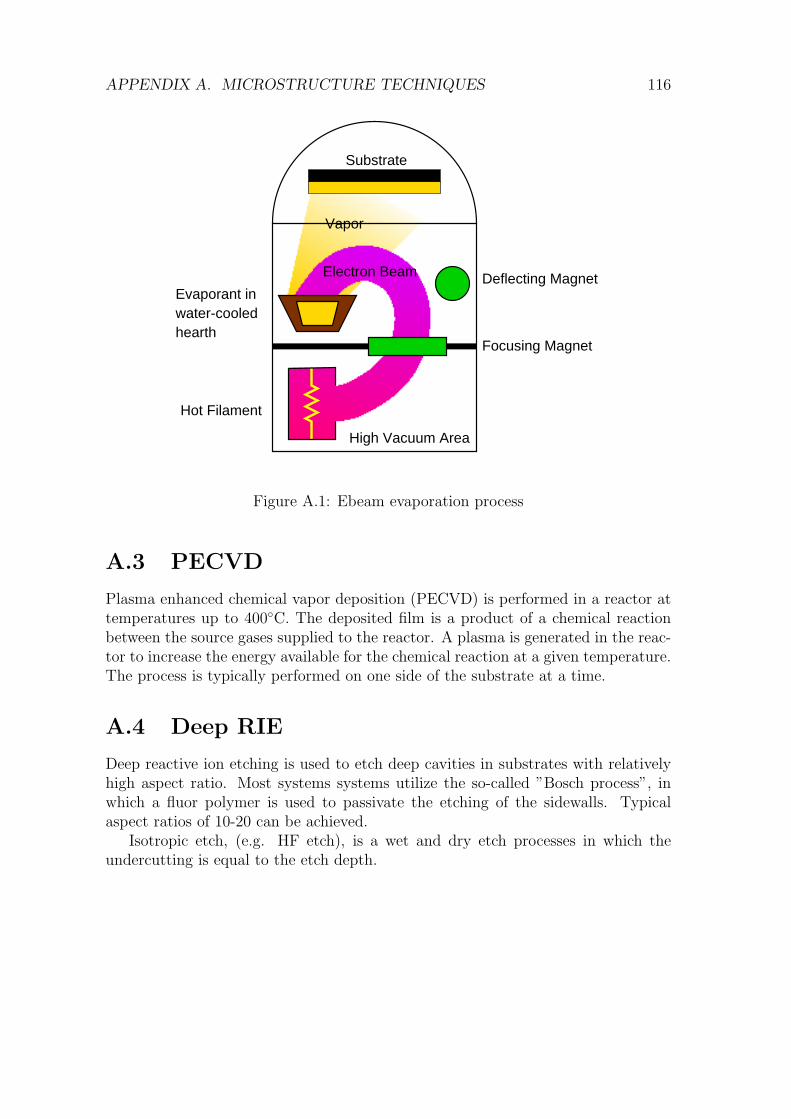
APPENDIX A. MICROSTRUCTURE TECHNIQUES 116
Evaporant inwater-cooledhearth
Deflecting Magnet
Focusing Magnet
High Vacuum Area
Substrate
Vapor
Electron Beam
Hot Filament
Figure A.1: Ebeam evaporation process
A.3 PECVD
Plasma enhanced chemical vapor deposition (PECVD) is performed in a reactor attemperatures up to 400C. The deposited film is a product of a chemical reactionbetween the source gases supplied to the reactor. A plasma is generated in the reac-tor to increase the energy available for the chemical reaction at a given temperature.The process is typically performed on one side of the substrate at a time.
A.4 Deep RIE
Deep reactive ion etching is used to etch deep cavities in substrates with relativelyhigh aspect ratio. Most systems systems utilize the so-called ”Bosch process”, inwhich a fluor polymer is used to passivate the etching of the sidewalls. Typicalaspect ratios of 10-20 can be achieved.
Isotropic etch, (e.g. HF etch), is a wet and dry etch processes in which theundercutting is equal to the etch depth.
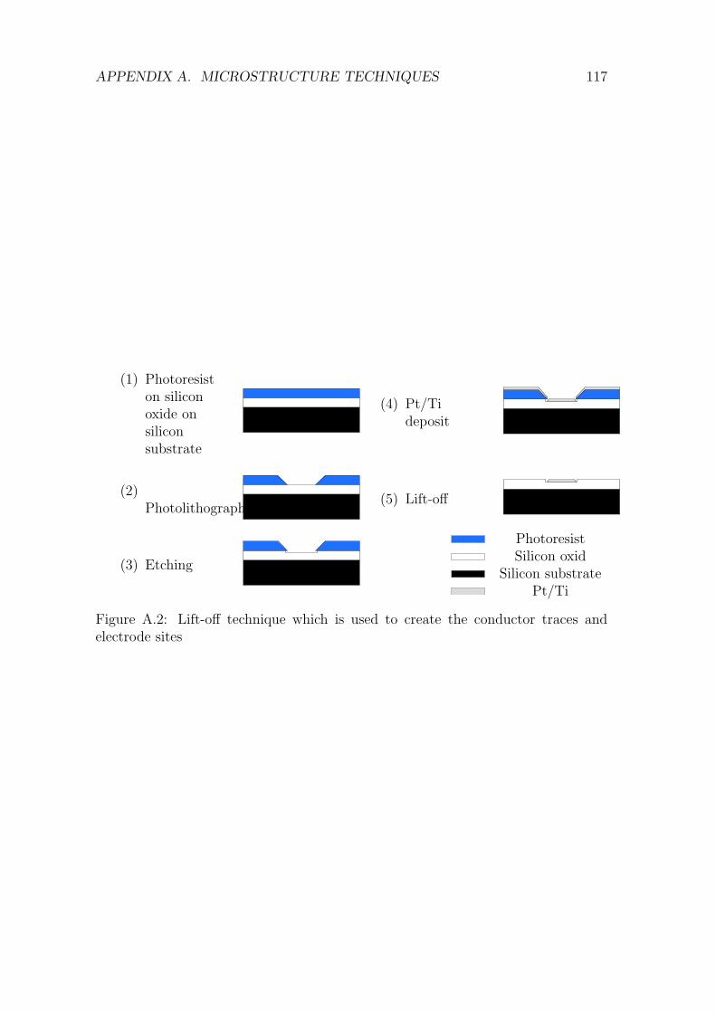
APPENDIX A. MICROSTRUCTURE TECHNIQUES 117
(1) Photoresiston siliconoxide onsiliconsubstrate
(4) Pt/Tideposit
(2)Photolithography
(5) Lift-off
(3) Etching
PhotoresistSilicon oxid
Silicon substratePt/Ti
Figure A.2: Lift-off technique which is used to create the conductor traces andelectrode sites
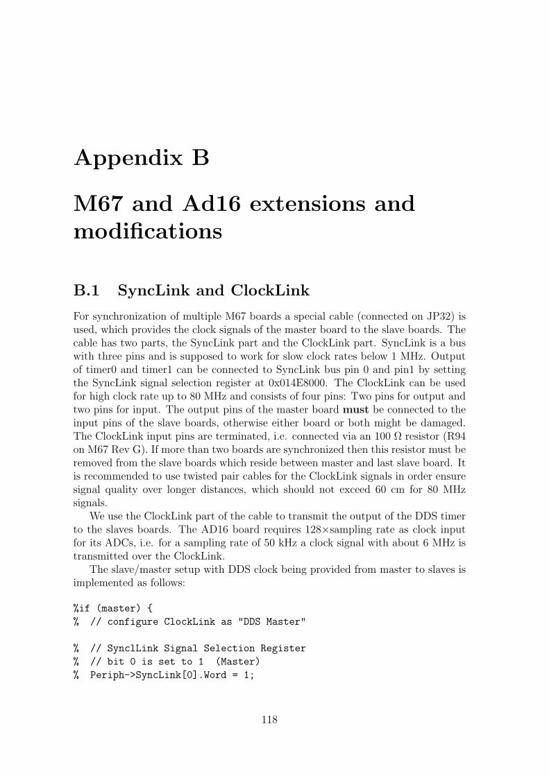
Appendix B
M67 and Ad16 extensions andmodifications
B.1 SyncLink and ClockLink
For synchronization of multiple M67 boards a special cable (connected on JP32) isused, which provides the clock signals of the master board to the slave boards. Thecable has two parts, the SyncLink part and the ClockLink part. SyncLink is a buswith three pins and is supposed to work for slow clock rates below 1 MHz. Outputof timer0 and timer1 can be connected to SyncLink bus pin 0 and pin1 by settingthe SyncLink signal selection register at 0x014E8000. The ClockLink can be usedfor high clock rate up to 80 MHz and consists of four pins: Two pins for output andtwo pins for input. The output pins of the master board must be connected to theinput pins of the slave boards, otherwise either board or both might be damaged.The ClockLink input pins are terminated, i.e. connected via an 100 Ω resistor (R94on M67 Rev G). If more than two boards are synchronized then this resistor must beremoved from the slave boards which reside between master and last slave board. Itis recommended to use twisted pair cables for the ClockLink signals in order ensuresignal quality over longer distances, which should not exceed 60 cm for 80 MHzsignals.
We use the ClockLink part of the cable to transmit the output of the DDS timerto the slaves boards. The AD16 board requires 128×sampling rate as clock inputfor its ADCs, i.e. for a sampling rate of 50 kHz a clock signal with about 6 MHz istransmitted over the ClockLink.
The slave/master setup with DDS clock being provided from master to slaves isimplemented as follows:
%if (master)
% // configure ClockLink as "DDS Master"
% // SynclLink Signal Selection Register
% // bit 0 is set to 1 (Master)
% Periph->SyncLink[0].Word = 1;
118
APPENDIX B. M67 AND AD16 EXTENSIONS AND MODIFICATIONS 119
Figure B.1: SyncLink/ClockLink cable pin documentation. Note the 100 Ω resistorwhich is integrated on the M67 board (Rev G) as resistor R94. This resistor ter-minates the ClockLink. But since more than one slave board is connected to theClockLinkOut pins like in this example, resistor R94 needs to be removed on theslave boards DSP 1 and DSP 2.
// SyncLink Destination Selection Register
// activate ClockLink
Periph->SyncLink[1].Word = 0;
else
// configure ClockLink as "DDS Slave",
// SynclLink Signal Selection Register
// bit 0 is set to 0 (Slave)
// bit 3 is set to 1 (get DDS from ClockLink)
Periph->SyncLink[0].Word = 8;
// SyncLink Destination Selection Register
// activate ClockLink
Periph->SyncLink[1].Word = 0;
APPENDIX B. M67 AND AD16 EXTENSIONS AND MODIFICATIONS 120
B.2 Synchronizing the AD16 boards
The synchronization of the ADCs of multiple AD16 boards is established by theso called AdcSync cable. A single wire which connects the SyncOut pin of oneAD16 board with the SynIn pin of the next AD16 board. All AD16 boards whichshould be synchronized are connected in a row by the AdcSync cable. In orderto activate synchronization the Innovative Integration library function AD16_sync
must be called for the first board in the row. The current implementation assumesthat this AD16 board resides in omnibus slot 0 of the master board.
B.3 Trigger Input
In many experiment settings a stimulus is presented to test subjects. The dataacquisition system should be able to acquire the time stamps of stimulus presentationtogether with the measured data. This requires that a stimulus generator can outputa TTL trigger signal, when it presents a stimulus. This trigger signal must beconnected to the M67 data acquisition hardware and then it possible to acquire thestimulus time stamps. There are different scenarios what kind of data is availablefrom a stimulus generator. It might have an digital port, where markers of differentstimuli are generated. How to use such data is sketched by the following paragraphs.
The external interrupt source line 3 of the C6701 which can be accessed on aomnibus connector pin can be utilized as trigger input line. A physical access pointmust customized by connecting pin 50 on the digital IO (DIO) port and pin 29 onJP 24 on the M67 board.
In order to support multiple external trigger lines, a circuit is required whichcombines the different trigger input line such that a single interrupt source is gen-erated for the DSP and for the DIO port clock input. In Figure B.2 this circuit isdenoted with ≥. Addtionally, the ”‘Edge to 1”’ circuit generates a logical 1 for eachactive trigger input line and it is connected to the pins of the DIO port. A fallingedge on the DIO port clock triggers that the DIO port latches all input lines intoits internal register. The digital input values must be stable for 10ns for latching.The same falling edge should trigger an interrupt service routine in the C6701 whichfetches the data from the internal DIO port register. This routine also stores a timestamp which is mapped onto a sample point index. As the time stamp is fetchedinside the interrupt service routine, the time resolution depends mainly on the inter-rupt latency. According to the C6701 documentation it takes 13 CPU cycles until aniterrupt service routine is executed. At 160MHz this corresponds to 87.5ns, whichis the ideal case. Actually, the latency depends on some other factors:
• Maximum number of instructions for which interrupts might be disabled,which happens in compiler generated code that utilizes software pipelining(see also compiler option -mi).
• DMA transfers, which have higher priority than the CPU to access memory,might increase the latency.
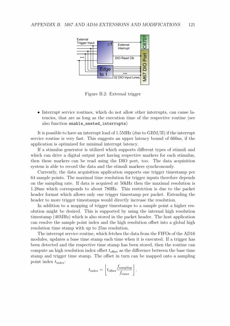
APPENDIX B. M67 AND AD16 EXTENSIONS AND MODIFICATIONS 121
External Trigger Input External
Interrupt≥1
M67
DIO
Por
t
DIO Read Clk
C67
01
Edgeto 1
32 DIO Input Lines
Figure B.2: External trigger
• Interrupt service routines, which do not allow other interrupts, can cause la-tencies, that are as long as the execution time of the respective routine (seealso function enable_nested_interrupts)
It is possible to have an interrupt load of 1.5MHz (due to GBM/II) if the interruptservice routine is very fast. This suggests an upper latency bound of 660ns, if theapplication is optimized for minimal interrupt latency.
If a stimulus generator is utilized which supports different types of stimuli andwhich can drive a digital output port having respective markers for each stimulus,then these markers can be read using the DIO port, too. The data acquisitionsystem is able to record the data and the stimuli markers synchronously.
Currently, the data acquisition application supports one trigger timestamp per64 sample points. The maximal time resolution for trigger inputs therefore dependson the sampling rate. If data is acquired at 50kHz then the maximal resolution is1.28ms which corresponds to about 780Hz. This restriction is due to the packetheader format which allows only one trigger timestamp per packet. Extending theheader to more trigger timestamps would directly increase the resolution.
In addition to a mapping of trigger timestamps to a sample point a higher res-olution might be desired. This is supported by using the internal high resolutiontimestamp (40MHz) which is also stored in the packet header. The host applicationcan resolve the sample point index and the high resolution offset into a global highresolution time stamp with up to 25ns resolution.
The interrupt service routine, which fetches the data from the FIFOs of the AD16modules, updates a base time stamp each time when it is executed. If a trigger hasbeen detected and the respective time stamp has been stored, then the routine cancompute an high resolution index offset toffset as the difference between the base timestamp and trigger time stamp. The offset in turn can be mapped onto a samplingpoint index tindex:
tindex =
⌊toffset
fsampling
ftimer
⌋.
Appendix C
Realtime operating system
C.1 Overview
Realtime Operating Systems (RTOS) are special kinds of operating systems. Atlarge an RTOS provides a robust, high performance software architecture on whichhigher level software applications can be developed. In contrast to a gerneral pur-pose operating system (GPOS) an RTOS provides deterministic behaviour of basicservices, which usually include
• task scheduling,
• intertask communication,
• sychronization,
• dynamic memory allocation, and
• timer services.
Deterministic behaviour is particularly important for embedded systems interactingwith the real world. Such systems need to react on events within a strict time dead-line, which is usually short, regardless of whatever happens in the system, i.e. howmany other tasks are running or messages are transmitted. In an RTOS the timeand resources needed to execute an operating system service are known and theyare limited, such that there are no random timing components. Random elementsin service times would cause random delays in application software and would thenmake the application randomly miss real-time deadlines, which is unacceptable for areal-time system. GPOSs (such as Windows or Linux) are usually non-deterministic,e.g. moving a window influences the response or execution time of other applica-tions. Furthermore, timing resolution is not as high as often necessary in embeddedapplications.
There are a number of commercial benefits when using an off the shelve RTOS fordevelopment of an real time application. Instead of implementing proprietary equiv-alents of the basic operating system services one can use proven and well documentedfunctionality of the RTOS. Moreover, having such a foundation for an application
122
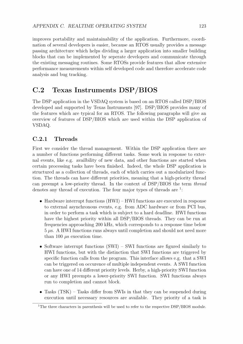
APPENDIX C. REALTIME OPERATING SYSTEM 123
improves portability and maintainability of the application. Furthermore, coordi-nation of several developers is easier, because an RTOS usually provides a messagepassing architecture which helps dividing a larger application into smaller buildingblocks that can be implemented by seperate developers and communicate throughthe existing messaging routines. Some RTOSs provide features that allow extensiveperformance measurements within self developed code and therefore accelerate codeanalysis and bug tracking.
C.2 Texas Instruments DSP/BIOS
The DSP application in the VSDAQ system is based on an RTOS called DSP/BIOSdeveloped and supported by Texas Instruments [97]. DSP/BIOS provides many ofthe features which are typical for an RTOS. The following paragraphs will give anoverview of features of DSP/BIOS which are used within the DSP application ofVSDAQ.
C.2.1 Threads
First we consider the thread management. Within the DSP application there area number of functions performing different tasks. Some work in response to exter-nal events, like e.g. availbility of new data, and other functions are started whencertain processing tasks have been finished. Indeed, the whole DSP application isstructured as a collection of threads, each of which carries out a modularized func-tion. The threads can have different priorities, meaning that a high-priority threadcan preempt a low-priority thread. In the context of DSP/BIOS the term threaddenotes any thread of execution. The four major types of threads are 1:
• Hardware interrupt functions (HWI) – HWI functions are executed in responseto external asynchronous events, e.g. from ADC hardware or from PCI bus,in order to perform a task which is subject to a hard deadline. HWI functionshave the highest priority within all DSP/BIOS threads. They can be run atfrequencies approaching 200 kHz, which corresponds to a response time below5 µs. A HWI functions runs always until completion and should not need morethan 100 µs execution time.
• Software interrupt functions (SWI) – SWI functions are figured similarly toHWI functions, but with the distinction that SWI functions are triggered byspecific function calls from the program. This interface allows e.g. that a SWIcan be triggered on occurence of multiple independent events. A SWI functioncan have one of 14 different priority levels. Herby, a high-priority SWI functionor any HWI preempts a lower-priority SWI function. SWI functions alwaysrun to completion and cannot block.
• Tasks (TSK) – Tasks differ from SWIs in that they can be suspended duringexecution until necessary resources are available. They priority of a task is
1The three characters in parenthesis will be used to refer to the respective DSP/BIOS module.
APPENDIX C. REALTIME OPERATING SYSTEM 124
SoftwareInterrupts
(SWI)14 levels
Tasks(TSK)
15 levels
Background
(IDL)Thread
HardwareInterrupts
(HWI)
Prio
rity
Figure C.1: Thread priorities
always lower than the priority of SWIs or HWIs. Additionally, there are 15different priority levels available for prioritization within tasks. For communi-cation and synchronization within tasks and with SWIs or HWIs a number ofstructures including queues, semaphores, and mailboxes can be employed.
• Background thread (IDL) – In the background thread the idle loop is exe-cuted, which continuously runs except when it is preempted by another higher-priority thread. Functions that are not subject to any hard deadline can berun within the idle loop. However, since each function is called after the pre-vious has been finished, they should not block, because otherwise they wouldprevent other idle loop functions from being executed.
Figure C.1 illustrates priority levels of the different thread types.
C.2.2 Interthread communication and synchronization
As already mentioned above DSP/BIOS has different structures to enable interthreadcommunication and synchronization:
• Semaphores (SEM) – Semaphores are often used to coordinate access to ashared resource among a set of competing tasks. Basically, a semaphore isa counter which comes together with atomic operations for incrementing anddecrementing. The value of the counter corresponds to the number of availableresources. Thus the counter of the semaphore can only be decremented if itis greater than zero. Before a task accesses a ressource it needs to acquire therespective semaphore (decrementing). The task is blocked if the semaphorecounter is zero. In this case DSP/BIOS additionaly supports different timeout
APPENDIX C. REALTIME OPERATING SYSTEM 125
mechanisms, i.e. the acquisition of the semaphore fails immediately, aftera certain period of time, or never, meaning that the task blocks until thesemaphore becomes available. When the ressource is not longer used, the taskmust release the semaphore (incrementing).
• Mailboxes (MBX) – A set of functions provides a mailbox functionality wheremessages are of fixed length and the number of messages is also fixed. Taskscan only post messages if there is a free slot in the mailbox. Otherwise theycan wait for a certain timeout period or until a slot becomes available. Withsuch a mailbox mechanism one can prevent an application being flooded bymore messages, than it can handle. On the other hand a task can wait formessages to be posted into a mailbox, again for a certain timeout period oruntil a message is available.
• Queues (QUE) – Queues can be used to exchange data structures of arbitrarylength and number between threads. Queue elements can be added and re-moved by atomic operations. Usually queues are used in a FIFO (First In FirstOut) sense, i.e. elements are inserted at the tail and removed at the head ofthe queue. However, insertion and removal of elements at arbitrary positionsof the queue is also possible.
C.2.3 Timer
DSP/BIOS has two different time services – a system clock and a high- and low-resolution timer. By default, the low-resolution time is equal to the system clock.However, any other event, such as availability of data, can also be the time basefor the system clock. Moreover, low- and high-resolution timer can be disabled orenabled. Using one of the on-device timers as time base for low- and high-resolutionsclocks a time resolution close to single instructions cycles is supported.
C.2.4 Profiling
DSP/BIOS provides statistic objects (STS) which compute the sum, mean, andmaximum for a series of data during execution of the program. The results aredisplayed within CCS. Based on the timer services one can measure execution timesof algorithms, and thus determine if time deadlines are meet by a specific part ofthe code. STS objects can also be employed in order to measure the needed amountof memory on the stack, or to check plausibility of acquired or processed data.

List of Figures
1.1 Overview of the project VSAMUEL . . . . . . . . . . . . . . . . . . . 2
2.1 Basic neuron . . . . . . . . . . . . . . . . . . . . . . . . . . . . . . . . 62.2 Morphological neural cell categorization . . . . . . . . . . . . . . . . . 82.3 Layered structure of cerebral cortex . . . . . . . . . . . . . . . . . . . 102.4 Layered structure of the cerebellum . . . . . . . . . . . . . . . . . . . 112.5 Scheme of an action potential . . . . . . . . . . . . . . . . . . . . . . 132.6 Connection between field and action potentials. . . . . . . . . . . . . 142.7 Tuning curve . . . . . . . . . . . . . . . . . . . . . . . . . . . . . . . 15
3.1 Interceptable neural activity . . . . . . . . . . . . . . . . . . . . . . . 183.2 Equivalent circuit for a biopotential electrode . . . . . . . . . . . . . 193.3 Extracellular recording and gap resistance . . . . . . . . . . . . . . . 213.4 Microelectrodes with single tip. . . . . . . . . . . . . . . . . . . . . . 223.5 MEA probe and needle array. . . . . . . . . . . . . . . . . . . . . . . 233.6 Michigan probe . . . . . . . . . . . . . . . . . . . . . . . . . . . . . . 233.7 SEM of VSAMUEL probe E4 . . . . . . . . . . . . . . . . . . . . . . 243.8 VSAMUEL Probes . . . . . . . . . . . . . . . . . . . . . . . . . . . . 253.9 Manufacturing process of the VSAMUEL probes . . . . . . . . . . . . 26
4.1 General attenuation scheme of a filter . . . . . . . . . . . . . . . . . . 284.2 Comparison of frequency responses of high pass IIR and FIR filter. . 314.3 IIR and FIR high pass filter . . . . . . . . . . . . . . . . . . . . . . . 324.4 Single level decomposition and reconstruction filter bank . . . . . . . 334.5 Wavelet filter bank of depth three . . . . . . . . . . . . . . . . . . . . 344.6 High pass filter using a wavelet filter bank . . . . . . . . . . . . . . . 344.7 Variance of WFB filter in frequency domain due to translation . . . . 354.8 Efficient implementation of an FIR filter followed by a subsampler . . 374.9 Efficient implementation of upsampling with subsequent FIR filter . . 374.10 One stage wavelet filter bank in term of polyphase matrices. . . . . . 384.11 Wavelet coefficients in lifting order . . . . . . . . . . . . . . . . . . . 484.12 Lifting prediction step in linear assembler . . . . . . . . . . . . . . . . 49
5.1 High pass filter implemented with a wavelet filter bank . . . . . . . . 525.2 Denoising of a neural recording . . . . . . . . . . . . . . . . . . . . . 545.3 Histograms of extracted noise of a neural recording . . . . . . . . . . 545.4 Comparison of denoising results using different wavelets . . . . . . . . 55
126
LIST OF FIGURES 127
5.5 NEO operator applied to neural recording . . . . . . . . . . . . . . . 565.6 NEO operator applied to neural recording . . . . . . . . . . . . . . . 565.7 Spike snippets, wavelet based features, and scalograms of the same
single spike snippet at different translations . . . . . . . . . . . . . . 605.8 Translation variance of the energy feature . . . . . . . . . . . . . . . 61
6.1 Data acquisition system hardware setup . . . . . . . . . . . . . . . . 656.2 Design of the VSAMUEL probe E3 . . . . . . . . . . . . . . . . . . . 666.3 Pre and main amplifier for 64 channels . . . . . . . . . . . . . . . . . 686.4 Basic concept of sigma-delta converter, [1] . . . . . . . . . . . . . . . 706.5 AD16 board . . . . . . . . . . . . . . . . . . . . . . . . . . . . . . . . 716.6 M67 board equipped with AD16 and its installed heat spreader . . . 716.7 DMA controller configuration registers . . . . . . . . . . . . . . . . . 736.8 Datapath from AD16 to PCI bus . . . . . . . . . . . . . . . . . . . . 746.9 Host PC of data acquisition system with 128 channels . . . . . . . . . 756.10 Adapter board for analog input SCSI to Latch. . . . . . . . . . . . . 766.11 Additional fans and airholes in the cabinet. . . . . . . . . . . . . . . . 766.12 Small cabinet with improved air flow . . . . . . . . . . . . . . . . . . 776.13 Packet management within DSP application . . . . . . . . . . . . . . 786.14 Communication channels between host and target . . . . . . . . . . . 806.15 Data Transfer Protocol . . . . . . . . . . . . . . . . . . . . . . . . . . 816.16 Main Panel . . . . . . . . . . . . . . . . . . . . . . . . . . . . . . . . 826.17 Configure a new experiment . . . . . . . . . . . . . . . . . . . . . . . 846.18 Probe and site group settings . . . . . . . . . . . . . . . . . . . . . . 866.19 Probe setup dialog . . . . . . . . . . . . . . . . . . . . . . . . . . . . 876.20 Amplifier setup dialog . . . . . . . . . . . . . . . . . . . . . . . . . . 876.21 Blueplot . . . . . . . . . . . . . . . . . . . . . . . . . . . . . . . . . . 886.22 Spectrogram in time frequency mode . . . . . . . . . . . . . . . . . . 896.23 Spectrogram in waterfall mode . . . . . . . . . . . . . . . . . . . . . . 896.24 Scope with open setup context menu . . . . . . . . . . . . . . . . . . 906.25 Menu of tool button . . . . . . . . . . . . . . . . . . . . . . . . . . . 916.26 Add Analyzer dialog . . . . . . . . . . . . . . . . . . . . . . . . . . . 926.27 Wavelet filter setup dialog . . . . . . . . . . . . . . . . . . . . . . . . 936.28 Wavelet denoising setup . . . . . . . . . . . . . . . . . . . . . . . . . 936.29 Wavelet denoising and Wavelet filtering . . . . . . . . . . . . . . . . . 946.30 Class diagram for VSFileReader and VSFileWriter . . . . . . . . . . . 956.31 Classes for data acquisition from multiple DSP boards. . . . . . . . . 966.32 Interaction of classes during data acquisition. . . . . . . . . . . . . . 976.33 Merging of raw data from three DSP applications. . . . . . . . . . . . 996.34 Reorder of acquired data after copy from shared memory . . . . . . . 1006.35 Class diagram for VSRingBuffer and VSDataBuffer . . . . . . . . . . 1016.36 Classes for data distribution . . . . . . . . . . . . . . . . . . . . . . . 102
7.1 Field potential profiles obtained in the medial entorhinal cortex . . . 1047.2 Simultaneous recording from 4 sites after induction of fast gamma
oscillations . . . . . . . . . . . . . . . . . . . . . . . . . . . . . . . . . 105

LIST OF FIGURES 128
7.3 Single unit recordings performed with a M2 probe . . . . . . . . . . . 1067.4 Field potential profile . . . . . . . . . . . . . . . . . . . . . . . . . . . 1077.5 Receptive fields in Crus II and PML . . . . . . . . . . . . . . . . . . 1087.6 Multi unit recording in cerebellum . . . . . . . . . . . . . . . . . . . . 1087.7 Extracellular action potential recorded in rat cerebellum . . . . . . . 1097.8 Spike interval histogram of evoked activity in rat cerebellum . . . . . 109
A.1 Ebeam evaporation process . . . . . . . . . . . . . . . . . . . . . . . 116A.2 Lift-off technique . . . . . . . . . . . . . . . . . . . . . . . . . . . . . 117
B.1 SyncLink/ClockLink cable . . . . . . . . . . . . . . . . . . . . . . . . 119B.2 External trigger . . . . . . . . . . . . . . . . . . . . . . . . . . . . . . 121
C.1 Thread priorities . . . . . . . . . . . . . . . . . . . . . . . . . . . . . 124

Bibliography
[1] Analog Devices. Sigma-Delta ADCs and DACs. search for AN-283 on http:
//www.analog.com.
[2] Gerardo Biella and Marco de Curtis. Olfactory inputs activate the medialentorhinal cortex via the hippocampus. Journal of Neurophysiology, 83:1924–1931, 2000.
[3] Gerardo Biella, Laura Uva, Ulrich G. Hofmann, and Marco de Curtis. As-sociative potentials in the entorhinal cortex of the guinea pig. Journal ofNeurophysiology, 88:1159–65, 2002.
[4] Gerardo Biella, Laura Uva, Ulrich G. Hofmann, and Marco de Curtis. In-trinsic and associative synaptic circuit in the temporal neocortex, perirhinaland enotrhinal cortex: an intra- and extracellular electrophysiological study.Forum of European Neurosciences - Abstracts, 2002.
[5] B. Black. Analog-to-digital converter architectures and choices for systemdesign. Analog Dialogue, 33(8), September 1999.
[6] J.O. Bockris and S.U.M. Khan. Surface Electrochemistry: A Molecular LevelApproach. Plenum Press, New York, June 1993.
[7] Andrew P. Bradley. Shift-invariance in the discrete wavelet transform. InProc. VIIth Digital Image Computing: Techniques and Applications, pages29–38, Sydney, December 2003.
[8] Joseph D. Bronzino, editor. The Biomedical Engineering Handbook, volume 1.CRC Press and IEEE Press, 2 edition, 2000.
[9] B.H. Brown, R.H. Smallwood, D.C. Barber, P.V. Lawford, and D.R. Hose.Medical Physics and Biomedical Engineering. Series in Medical Physics. Insti-tute of Physics Publishing, Bristol and Philadelphia, 1999.
[10] P.K. Campbell, R. A. Normann, K.W. Horch, and S. S. Stensaas. A chronicintracortical electrode array: Preliminary results. J. Biomed. Mats. Res.:Applied Biomats, 23:245 – 259, 1989.
[11] S. Grace Chang, Bin Yu, and Martin Vetterli. Adaptive wavelet thresholdingfor image denoising and compression. IEEE Transactions on Image Processing,9(9), September 2000.
129
BIBLIOGRAPHY 130
[12] Enric Claverol-Tinture and Jerry Pine. Extracellular potentials in low-densitydissociated neuronal cultures. Journal of Neuroscience Methods, 117(1):13–21,2002.
[13] I. Daubechies. Orthonormal bases of compactly supported wavelets. Commu-nications on Pure and Applied Mathematics, 41:909–996, 1988.
[14] I. Daubechies and W. Sweldens. Factoring wavelet transforms into liftingsteps. J. Fourier Anal. Appl., 4(3):245–267, 1998.
[15] Peter Dayan and L.F. Abbott. Theoretical Neuroscience: Computational andMathematical Modeling of Neural Systems. MIT Press, 1 edition, December2001.
[16] Marco de Curtis, Gerardo Biella, C. Buccellati, and G. Folco. Simultaneousinvestigation of the neuonal and vascular compartments in the guinea pig brainisolated in vitro. Brain Research Protocols, 3(2):221–228, 1998.
[17] Marco de Curtis and Ulrich G. Hofmann. Development of a versatile systemfor advanced neuronal recordings with multi-site microelectrodes. Technicalreport, Istituto Nazionale Neurologico ”Carlo Besta”, Milano, Italy, February2003.
[18] Marco de Curtis, D Pare, and R Llinas. The electrophysiology of the olfactoryhippocampal system in the isolated and perfused adult mammalian brain invitro. Hippocampus, 1(4):341–354, 1991.
[19] Clayton T. Dickson, Gerardo Biella, and Marco de Curtis. Evidence for spatialmodules mediated by temporal synchronization of carbachol-induced gammarhythm in medial entorhinal cortex. Journal of Neuroscience, 20:7846–7854,2000.
[20] Clayton T. Dickson, Gerardo Biella, and Marco de Curtis. Enhancement ofspatial and temporal synchronization in the enthorinal cortex by phase reset.Hippocampus, 12(4):447–456, 2002.
[21] David L. Donoho. De-noising by soft-thresholding. IEEE Transactions onInformation Theory, 41(3):613–627, 1995.
[22] David L. Donoho and Iain M. Johnstone. Ideal spatial adaptation by waveletshrinkage. Biometrika, 81(3):425–455, 1994.
[23] David L. Donoho and Iain M. Johnstone. Adapting to unknown smooth-ness via wavelet shrinkage. Journal of the American Statistical Association,90(432):1200–1224, 1995.
[24] Alpha Omega Engineering. Alpha map data acquisition system. Brochure onwebsite, 2008.

BIBLIOGRAPHY 131
[25] P. Fagerstedt and E. DeSchutter. Multi-layer recordings from the cerebellarcortex of the anestethetized rat using multi-site silicon probes. Forum ofEuropean Neurosciences - Abstracts, page 15, 2004. A129.4.
[26] P. Fagerstedt, A. Volny-Luraghi, M. Kindlundh, P. Norlin, U. G. Hofmann,and E. De Schutter. Novel silicon probes with multi-site microelectrodes forsingle unit and local field potential (lfp) recordings from cerebellar cortex ofanesthetized rats. Forum of European Neurosciences - Abstracts, 2002. A126.8.
[27] Patriq Fagerstedt, Antonia Volny-Luraghi, and Erik De Schutter. Results ofin vivo acute recordings from cerebellum. Technical report, Laboratory ofTheoretical Neurobiology, University of Antwerp, August 2003.
[28] A. Folkers and U.G. Hofmann. Data acqusition system for 32 channels.VSAMUEL Deliverable Report 4.1, ISIP, University of Lubeck, dec 2002.
[29] A. Folkers and U.G. Hofmann. Data acqusition system for 64 channels includ-ing compression schemes. VSAMUEL Deliverable Report 4.2, ISIP, Universityof Lubeck, May 2002.
[30] A Folkers, S Jannasch, and U.G. Hofmann. Lifting scheme - an alternative towavelet transforms for real time applications. GlobalDSP Magazine, 2(12):3–6,dec 2003.
[31] A. Folkers, H Stemman, K.M.L. Menne, P. Norlin, M. Kindlundh, W. Frei-wald, and U.G. Hofmann. Realtime wavelet-based clustering for a 64 channelmultisite recording system. In CNS’03, page abstract and Poster, 2003.
[32] Andre Folkers and Ulrich G. Hofmann. A multichannel data acquisition andanalysis system based on off-the-shelf dsp boards. In Kalman Fazekas, editor,Proceedings of the EURASIP Conference on Digital Signal Processing for Mul-timedia Communications and Services, pages 249–252, Budapest, September2001. EURASIP, Scientific Association of Infocommunications - HTE. ISBN963-8111-64-X.
[33] Andre Folkers, Florian Mosch, Thomas Malina, and Ulrich G. Hofmann. Real-time bioelectrical data acquisition and processing from 128 channels utilizingthe wavelet-transformation. Neurocomputing, 52–54:247–254, 2003.
[34] W. Freiwald, H. Stemmann, A. Wannig, A. K. Kreiter, U. G. Hofmann, M. D.Hills, G. T. A. Kovacs, D. T. Kewley, J. M. Bower, C. W. Eurich, and S. D.Wilke. Stimulus representation in rat primary visual cortex: Multi-electroderecordings and estimation theory. Neurocomputing, 44–46:407–416, 2002.
[35] Winrich Freiwald, Heiko Stemmann, Aurel Wanning, Andreas K. Kreiter, Ul-rich G. Hofmann, Matthew D. Hills, Gregory T.A. Kovacs, David T. Kewley,James M. Bower, Axel Etzhold, Stefan D. Wilke, and Christian W. Eurich.Stimulus representation in rat primary visual cortex: multi-electrode record-ings with micromachined silicon probes and estimation theory. Neurocomput-ing, 44–46:407–416, 2002.
BIBLIOGRAPHY 132
[36] William F. Ganong. Review of Medical Physiology. Appleton & Lange, 17edition, 1995.
[37] Claude Ghez. Principles of Neural Science, chapter The Cerebellum, pages626–646. Appleton & Lange, 1991.
[38] Ghassan Gholmieh, Walid Soussou, Martin Hana, Ashish Ahuja, Min-ChiHsiao, Dong Songa, Armand R. Tanguay Jr., and Theodore W. Berger.Custom-designed high-density conformal planar multielectrode arrays forbrain slice electrophysiology. Journal of Neuroscience Methods, 152:116–129,2006.
[39] Multi Channel Systems MCS GmbH. ME System User Manual, 2006.
[40] Charles M. Gray, Pedro E. Maldonado, Mathew Wilson, and Bruce Mc-Naughton. Tetrodes markedly improve the reliability and yield of multiplesingle-unit isolation from multi-unit recordings in cate striate cortex. Journalof Neuroscience Methods, 63:43–54, 1995.
[41] J.A. Hartigan and M.A. Wong. A k-means clustering algorithm. AppliedStatistics, 28(1):100–108, 1979.
[42] G.H. Henry, B. Dreher, and P.O. Bishop. Orientation specificity of cells in catstriate cortex. Journal of Neurophysiology, 37:1394–1409, 1974.
[43] U.G. Hofmann, A. Folkers, F. F. Mosch, T. Malina, K.M.L. Menne, G. Biella,P. Fagerstedt, E. De Schutter, W. Jensen, K. Yoshida, D. Hoehl, U. Thomas,M.G. Kindlundh, P. Norlin, and M. De Curtis. A novel high channel-count sys-tem for acute multisite neuronal recordings. IEEE Transactions on BiomedicalEngineering, 53(8):1672 – 1677, 2006.
[44] U.G. Hofmann, A Folkers, F Mosch, D Hohl, M Kindlundh, and P Norlin. A64(128)-channel multisite neuronal recording system. Biomedizinische Tech-nik, 47(E 1):194–197, 2002.
[45] U.G. Hofmann, Dirk Hohl, Andreas Hartlep, Robert Schmidt, Peter Detem-ple, Marion Bar, and Andre Folkers. Geschichtete rundumableitung neuronaleraktivitaten mittels koaxial gelagerter linearer oder helikaler mikroelektrode-nanordnungen, 2002.
[46] U.G. Hofmann, T. Malina, F. Mosch, K. Labusch, and A. Folkers. A versa-tile daq system for multisite recordings. In Society for Neuroscience Abstr.,volume 27, page Program No. 821.72, San Diego, 2001.
[47] Ulrich G. Hofmann, Erik De Schutter, Ken Yoshida, Marco De Curtis, UweThomas, and Peter Norlin. On the design of multi-site microelectrodes forneural recordings. In P. M. Knoll, editor, Proceedings of the MICRO.tec 2000,volume 1, pages 283 – 288, Berlin, 2000. VDE Verlag.

BIBLIOGRAPHY 133
[48] G.R. Holt and C. Koch. Electrical interactions via the extracellular potentialnear clell bodies. Journal of Computational Neuroscience, 6(2):169–184, 1999.
[49] S.D. Van Hooser, U.G. Hofmann, D.T. Kewley, and J.M. Bower. Relation-ship between field potentials and spike activity in rat s1: multi-site corticalrecordings and simulations. Neurocomputing, 32-33:591–596, 2000.
[50] M. Horikawa, H. Harada, and M. Yarita. Detection limit in low-amplitudeeeg measurement. Journal of Clincal Neurophysiology, 20(1):45–53, February2003.
[51] D.H. Hubel and T.N. Wiesel. Receptive fields and functional architecture ofthe monkey striate cortex. Journal of Physiology, 195:215–243, 1968.
[52] P. J. Huber. Robust Statistics. John Wiley and Sons, New York, 1981.
[53] Eyal Hulata, Ronen Segev, and Eshel Ben-Jacob. A method for spike sortingand detection based on wavelet packets and shannon’s mutual information.Journal of Neuroscience Methods, 117:1–12, 2002.
[54] IEEE. Programs for Digital Signal Processing. IEEE Press, New York, 1979.
[55] R.B. Illing. Geschichte der Hirnforschung. Lexikon der Neurowissenschaft,4:40–50, 2001.
[56] Innovative Integration, Thousand Oaks, California, USA. Multi-CardTiming Synchronization, 2001. m6x_synclink.pdf from http://www.
innovative-dsp.com.
[57] S. Jannasch, R. Klinger, N. Matter, and U. G. Hofmann. Recording elec-tromyographic signals in a classical conditioning experiment. In Short Articleand Poster, Jahrestagung der DGBMT, Ilmenau, 2004. Schiel & Schon.
[58] Herbert H. Jasper. The ten-twenty electrode system of the international feder-ation. Electroencephalography and clinical neurophysiology, 10:371–375, 1958.
[59] W. Jensen, K. Yoshida, and U.G. Hofmann. In-vivo implant mechanics offlexible, silicon-based acreo microelectrode arrays in rat cerebral cortex. IEEETransactions on Biomedical Engineering, 53(5):934–940, May 2006.
[60] W. Jensen, K. Yoshida, and U.G. Hofmann. In vivo implant mechanics ofsingle-shaft microelectrodes in peripheral nervous tissue. In Neural Engineer-ing, CNE ’07. 3rd International IEEE/EMBS Conference on, pages 1–4, 2007.
[61] Eric R. Kandel. Principles of Neural Science, chapter Nerve Cells and Be-haviour, pages 18–32. Appleton & Lange, 1991.
[62] Eric R. Kandel, James H. Schwartz, and Thomas M. Jessell, editors. Principlesof Neural Ncience. Appleton & Lange, 25 Van Zant Street, East Norwalk,Connecticut 06855, 3 edition, 1991.

BIBLIOGRAPHY 134
[63] Nick G. Kingsbury. The dual-tree complex wavelet transform: A newt tech-nique for shift invariance and directional filters. In Proc. 8th IEEE DSP Work-shop, Utah, August 1998. paper no. 86.
[64] John Koester. Principles of Neural Science, chapter Membrane Potential,pages 81–94. Appleton & Lange, 1991.
[65] G. Kreiman, C. Hung, A. Kraskov, R. Quiroga, T. Poggio, and J. DiCarlo.Object selectivity of local field potentials and spikes in the macaque inferiortemporal cortex. Neuron, 49:433–445, 2006.
[66] Abraham Kuruvilla and Roland Flink. Intraoperative electrocorticography inepilepsy surgery: useful or not? Seizure, 12(8):577–584, December 2003.
[67] Juan Carlos Letelier and Pamela P. Weber. Spike sorting based on discretewavelet transform coefficients. JNM, 101(2):93–106, September 2000.
[68] Michael S. Lewicki. Bayesian modeling and classification of neural signals.Neural Computation, 6(5):1005–1030, 1994.
[69] Michael S. Lewicki. A review of methods for spike sorting: the detection andclassification of neural action potentials. Network, 9(4):53–78, November 1998.
[70] Nikos Logothetis, Jon Pauls, Mark Augath, Torsten Trinath, and Axel Oelter-mann. Neurophysiological investigation of the basis of the fmri signal. Nature,412:150–157, 2006.
[71] T. Malina, A. Folkers, and U.G. Hofmann. Real-time eeg processing basedon wavelet transformation. In IFMBE Proceedings of the12th Nordic BalticConference on Biomedical Engineering and Medical Physics, pages 166–167,2002.
[72] T. Malina, A. Folkers, F. Mosch, K. Labusch, M. Schurmann, and U.G. Hof-mann. An integrated system to trigger feedback-coupled event related brainpotentials (erps). Biomedizinsche Technik, 46 E1:322–323, 2001.
[73] Stephane Mallat. A Wavelet Tour of Signal Processing. Academic Press, 2edition, 1999.
[74] McNaughton, O. Keefe, and Barnes. The stereotrode: A new technique forsimultaneous isolation of several single units in the central nervous system frommultiple unit records. Journal of Neuroscience Methods, 8:391–397, 1983.
[75] K.M.L. Menne, A. Folkers, R. Maex, T. Malina, and U.G. Hofmann. Testof spike sorting algorithms on the basis of simulated data. Neurocomputing,44–46:1119–1126, 2002. VSAMUEL.
[76] K.M.L. Menne, T Malina, A Folkers, and U.G. Hofmann. Biologically realisticsimulation of a part of hippocampal ca3: Generation of testdata for the evalu-ation of spike detection algorithms. In T. Martinetz D. Polani, J. Kim, editor,

BIBLIOGRAPHY 135
5th German Workshop on Artificial Life - Abstracting and Synthesizing thePrinciples of Living Systems, pages 17–25, Lubeck, 2002. IOS Press Infinix.
[77] K.M.L. Menne, H. Schuhart, A Folkers, and U. G. Hofmann. Neurosurgery bymultichannel electrophysiology, patient specific navigation, and customizeddatabase. In Dreilandertagung der Gesellschaft fur Biomedizinsche Technik2003, volume 48, pages 500–501, Salzburg, Austria, 2003. Schiele & Schon.
[78] Evangelia Micheli-Tzanakou. The Biomedical Engineering Handbook, vol-ume 1, chapter Nervous System. CRC Press and IEEE Press, 2 edition, 2000.
[79] M. Muhlethaler, Marco de Curtis, K. Walton, and R. Llinas. The isolated andperfused brain of the guinea pig in vitro. European J. Neuroscience, 5(7):915–926, 1993.
[80] S. Mukhopadhyay and G.C. Ray. A new interpretation of nonlinear energyoperator and its efficacyin spike detection. IEEE Transactions on BiomedicalEngineering, 45(2):180–187, 1998.
[81] Miguel A.L. Nicolelis, editor. Methods for neural ensemble recordings. CRCPress, 1999.
[82] Peter Norlin and Maria Kindlundh. Custom designed 32 microelectrode probes(VSAMUEL Deliverable 2.1). Technical report, ACREO AB, Kista, Sweden,May 2001.
[83] Peter Norlin, Maria Kindlundh, Aliette Mouroux, Ken Yoshida, and Ulrich G.Hofmann. A 32-site neural recording probe fabricated by drie of soi substrates.Journal of Micromechanics and Microengineering, 12:414–419, July 2002.
[84] Paul L. Nunez. Electric Field of the Brain: The Neurophysics of EEG. OxfordUniversity Press, New York, 1981.
[85] Paul L. Nunez and Ramesh Srinivasan. Electroencephalogram. Scholarpedia,2(2):1348, 2007.
[86] A.V. Oppenheim and R.W. Schafer. Discrete-time signal processing. signalprocessing series. Prentice Hall, 1989.
[87] L.R. Rabiner, J.H. McClellan, and T.W. Parks. Fir digital filter design tech-niques using weighted chebyshev approximations. Proc. IEEE, 63, 1975.
[88] M. Salganicoff, M. Sarna, L. Sax, and G.L. Gerstein. Unsupervised waveformclassification for multi-neural recordings: a real-time, software based system.i. algorithms and implementation. Journal of Neuroscience Methods, 25:181–187, 1988.
[89] Edward M. Schmidt. Methods for neural ensemble recordings, chapter Elec-trodes for many single neuronr recordings. CRC Press, 1999.
BIBLIOGRAPHY 136
[90] Erik De Schutter. Models. http://www.tnm.ua.ac.be/models/index.shtml,1998.
[91] Andrew B. Schwartz, X. Tracy Cui, Douglas J. Weber, and Daniel W. Moran.Brain-controlled interfaces: Movement restoration with neural prosthetics.Neuron, 52:205–220, October 2006.
[92] Ivan W. Selesnick, Richard G. Baraniuk, and Nick G. Kingsbury. The dual-treecomplex wavelet transform. IEEE Signal Processing Magazine, 22(6):123–151,November 2005.
[93] Ivan W. Selesnick and C.S. Burrus. Generalized digital butterworth filterdesign. Proceedings of the IEEE Int. Conf. Acoust., Speech, Signal Processing,3, May 1996.
[94] W. Singer and C.M. Gray. Visual feature integration and the temporal corre-lation hypothesis. Ann Rev Neurosci, 18:555–586, 1995.
[95] W. Sweldens. The lifting scheme: A new philosophy in biorthogonal waveletconstructions. In A. F. Laine and M. Unser, editors, Wavelet Applications inSignal and Image Processing III, pages 68–79. Proc. SPIE 2569, 1995.
[96] Plexon Neurotechnology Research Systems. Neural Data Acquisition System– Recorder/16 and Recorder/64, 2006.
[97] Texas Instruments Incorporated, Post Office Box 655303, Dallas, Texas75265. TMS320 DSP/BIOS User’s Guide, November 2001. http://www-s.ti.com/sc/psheets/spru423a/spru423a.pdf.
[98] H.D. Tong, R.A.F. Zwijze, J.W. Berenschot, R.J. Wiegerink, G.J.M. Krijnen,and M.C. Elwenspoek. Characterization of platinum lift-off technique. In Pro-ceedings of the Semiconductor Sensor Workshop, pages 697–702, Veldhoven,the Netherlands, December 2000. The Dutch Technology Foundation.
[99] M. Trepel. Neuroanatomie: Struktur und Funktion. Urban und Schwarzenberg,Munchen; Wien; Baltimore, 1995.
[100] Solange van der Linden, Ferruccio Panzica, and Marco de Curtis. Carbacholinduces fast oscillations in the medial but not in the lateral entorhinal cortexof the isolated guinea pig brain. Journal of Neurophysiology, 82:2441–2450,1999.
[101] A. Volny-Luraghi, R. Maex, B. Vos, and E. De Schutter. Peripheral stimuliexcite coronal beams of golgi cells in rat cerebellar cortex. Neuroscience,113(2):363–373, 2002.
[102] B. Weber, T. Malina, K. Menne, A. Folkers, V. Metzler, and Ulrich G. Hof-mann. Handling large files of multisite microelectrode recordings for the Eu-ropean VSAMUEL consortium. Neurocomputing, June 2001.

BIBLIOGRAPHY 137
[103] Wikipedia. Butterworth. Wikipedia, 2007. http://en.wikipedia.org/wiki/Butterworth_filter.
[104] Menno Witter and Floris Wouterlood, editors. The Parahippocampal Region:Organization and Role in Cognitive Functions. Oxford University Press, NewYork, 2002.
[105] S. Ramon y Cajal. Histology. Wood, 10 edition, 1933.
[106] Ken Yoshida, W. Jensen, Peter Norlin, M. Kindlundh, and Ulrich G. Hofmann.Characterization of silicon microelectrodes from the EU VSAMUEL project.In J. Werner, editor, Biomedizinsche Technik, Bochum, 2001. Schiele & SchonGmbH.

Lebenslauf
Andre Folkers
Kontakt Pausheide 933415 [email protected]
Personliche Daten
geboren am 14. Januar 1974 in WesterstedeFamilienstand verheiratet seit 26.11.1999
mit Dr. med. Verena Folkers, geb. SpringfeldKinder Antonia, Karolin, Frederik und Teresa
Berufstatigkeit
18. Mai 2009 Doktorprufung zum Dr.-Ing. an der Universitat zu Lubeckseit 01/2007 Softwareentwickler bei Beckhoff Automation GmbH, Verl
10/2003 – 12/2006 Softwareentwickler bei Harman/Becker Automotive Systems,Hamburg
02/2003 – 09/2003 Software-Ingenieur bei Thomas Recording GmbH, Gießen,in Kooperation mit der Universitat Lubeck
02/2000 – 01/2003 Wissenschaftlicher Mitarbeiter am Institut fur Signalverarbeitung,Universitat zu Lubeck
Studium und Schule
10/1994 – 01/2000 Informatik mit Nebenfach Medizinische Informatik,Universitat zu Lubeck
14. Januar 2000 Diplom in Informatik04/1999 – 09/1999 Diplomarbeit
”Pictorial Query Specification and Processing“
Universitat von Maryland in College Park, USA7. Oktober 1996 Vordiplom
02/1996 – 12/1998 Studentischer Mitarbeiter am Institut fur Technische Informatik04/1997 – 07/1997 Studentischer Ubungsleiter am Institut fur Informationssysteme10/1996 – 02/1997 Studentischer Mitarbeiter am Institut fur Mathematik10/1993 – 09/1994 Sanitatssoldat, Sanitatsbataillon 11, Leer und Varel
3. Mai 1993 Abitur am Gymnasium Westerstede
Related Documents