DARTPIV: Dynamic Adaptive Real-Time Particle …groups.csail.mit.edu/robotics-center/public_papers/Sharma13.pdfDARTPIV: Dynamic Adaptive Real-Time Particle ... Dynamic Adaptive Real-Time

1

DARTPIV: Dynamic Adaptive Real-Time Particle

Image Velocimetry

by

Samvaran Sharma

Submitted to the Department of Electrical Engineering and Computer Science

In partial fulfillment of the requirements for the degree of

Master of Engineering

At the

MASSACHUSETTS INSTITUTE OF TECHNOLOGY

May 2013

© Massachusetts Institute of Technology 2013. All rights reserved.

Signature of Author………………………………………………………………………………………………

Department of Electrical Engineering and Computer Science

May 23, 2013

Certified by………………………………………………………………………………………………………….

Professor Russ Tedrake

Associate Professor of Computer Science, CSAIL

Thesis Supervisor

Accepted by…………………………………………………………………………………………………………

Professor Dennis M. Freeman

Chairman, Masters of Engineering Thesis Committee

2

3

DARTPIV: Dynamic Adaptive Real-Time Particle Image

Velocimetry

by

Samvaran Sharma

Submitted to the Department of Electrical Engineering and Computer Science in partial

fulfillment of the requirements for the degree of

Master of Engineering

Abstract

Particle Image Velocimetry (PIV) is a technique that allows for the detailed

visualization of fluid flow. By performing computational analysis on images taken by a

high-sensitivity camera that monitors the movement of laser-illuminated tracer particles

over time, PIV is capable of producing a vector field describing instantaneous velocity

measurements of the fluid captured in the field of view. Nearly all PIV implementations

feature offline processing of the collected data, a feature that limits the scope of the

applications of this technique. Recently, however, researchers have begun to explore the

possibility of using FPGAs or PCs to greatly improve the efficiency of these algorithms

in order to obtain real-time speeds for use in feedback loops. Such approaches are very

promising and can help expand the use of PIV into previously unexplored fields, such as

robot locomotion. Yet these real-time algorithms have the potential to be improved even

further. This thesis outlines an approach to make real-time PIV algorithms more

accurate and versatile in large part by applying principles from another emerging

technique called adaptive PIV, and in doing so will also address new issues created from

the conversion of traditional PIV to a real-time context. This thesis also documents the

implementation of this Dynamic Adaptive Real-Time PIV (DARTPIV) algorithm on a

PC with CUDA parallel computing, and its performance and results analyzed in the

context of normal real-time PIV.

Thesis Supervisor: Russ Tedrake

Title: Associate Professor of Computer Science, CSAIL

4

5

Acknowledgements

My journey at MIT has been a long one

6

[blank]

7

[TABLE OF CONTENTS 1]

8

[TABLE OF CONTENTS 2]

9

[TABLE OF CONTENTS 3]

10

[blank]

11

[LIST OF FIGURES]

12

[LIST OF FIGURES 2]

13

[LIST OF FIGURES 3]

14

[blank]

15

[LIST OF TABLES]

16

[blank]

17

Chapter 1

Introduction

Fluid-body systems pose a myriad of complex problems for researchers and designers in a

wide variety of fields. Control of a rigid body within the context of a freely-moving fluid is a

difficult problem to model, and thus a difficult one to solve, particularly when given very

short time scales to work with. Even a cursory glance into the details of this topic will

reveal several unique challenges: first, the fluid state at any given time is difficult to

ascertain not only because of its complex nature, but also due to the simple fact that they

are difficult to visualize; second, in order to fill out gaps in the visualization or project

forward into time, it is necessary to develop a model that will accurately describe how the

complex flow will evolve, which is both difficult to ascertain for every potential flow

condition, and computationally intensive to complete; third, in the context of control, any

approach that must be taken must be responsive over a very short time scale so as to be

useful as an input in a feedback loop.

18

Given the difficult nature of these problems, it may be appropriate to ask whether it

is worthwhile pursuing these challenges, as it is perfectly possible to create control schemes

that do not take into account the state of the fluid. However, in doing so, we would be

passing over a great opportunity to convert a persistent foe into a valuable ally – namely,

ignoring the potential benefits we could obtain from recognizing and capitalizing on fluid

state to accomplish control tasks. In nature, animals have long since evolved techniques to

take advantage of the fluid state around them, not only physiologically (through wing

shape, body shape, and effective natural control surfaces), but also mentally, by learning

through experience. In the same way humans have become exceedingly efficient walkers,

using the momentum of our own bodies to make the task more efficient rather than fighting

against it, birds, bees, bats, and fish have, for millennia, become masters of using the

subtleties of the medium that transports them to their advantage.

Yet perhaps the more practical and compelling reason is that the need for solving

such problems is increasing. With the rapid rise of interest in Micro Air Vehicles (MAVs)

and continued research in underwater robotics, it is becoming increasingly desirable to find

a way to more gracefully deal with fluid structures and use them to increase locomotive

efficiency, as opposed to attempting to simply overpower their effects and compensate for

the error between the robot’s desired state and measured state.

One approach that can offer answers to the problem of visualization is a technique

called Particle Image Velocimetry (PIV), which can reveal a vector field approximating the

nature of the fluid flow by tracking particles suspended in a transparent liquid. As these

particles are carried around by the flow structures, the motion of the fluid is revealed over

time, and captured and stored by a camera for later computational analysis.

While not a new approach, PIV has slowly but steadily spread in research

communities due to falling costs and a wider spread of knowledge. It has become a popular

method in many fields, including fluid dynamics and aerospace, amongst others, and has

19

even led to the creation of a small-yet-important industry around the technique, featuring

companies that sell commercial PIV systems or tailor-made components.

However, many of these setups continue to be relatively expensive, cumbersome, and

highly application-specific. While it is true that the general approach has been improved

upon, and new technologies have been incorporated in order to improve accuracy, efficiency,

and versatility, it is still possible for PIV to expand beyond its traditional spheres and lend

its capabilities to even more areas of research.

In order to marry the need for smarter, more efficient locomotive techniques in

robotics and control theory with the potential capabilities of particle image velocimetry, it

is necessary to bring PIV to a new level of fidelity by further leveraging cheap

computational power and novel approaches from recently published academic literature.

This paper outlines a method that seeks to improve upon established PIV practices in order

to improve and adapt the technique for use in a plethora of new settings, including robot

locomotion.

20

21

Chapter 2

Background and Objectives

2.1 How PIV Works

Particle Image Velocimetry has a short history borne out of a long-standing idea – that in

order to visualize the flow of a complex fluid, one can add tracer particles to it and study

the direction of the flow, in the same way one might drop a stick in a stream and take not

of the direction in which it is carried. Ludwig Prandtl, a German pioneer in the field of

aerodynamics, experimented with this concept in the early 20th century, using pieces of

aluminum to visualize the vortices created in the wake of a cylinder thrust into an otherwise

laminar flow.

PIV as we know it today originated in the 1980s. With work from researchers such

as Adrian, Laurenco and Krothapalli, Willert and Gharib, Westerweel, and many others,

the technique and its variants (such as Particle Tracking Velocimetry, Scalar Image

Velocimetry, and Image Correlation Velocimetry) began to develop academic clout and their

22

methodologies more refined. The use of digital photography led to a great leap forward in

PIV feasibility, which only improved as computers became faster and cheaper, and cameras

became more powerful and sensitive.

Today’s conventional PIV is accomplished by seeding a transparent fluid in a

transparent tank with highly reflective, neutrally-buoyant particles. Then, by utilizing a

laser sheet – that is, a laser beam spread into a 2-dimensional plane by a cylindrical lens –

pointed at the tank, one can light up a slice of the fluid, making the particles in that plane

shine brightly from the incoming light. A camera, whose line of sight is orthogonal to the

laser sheet, can then look into the tank and rapidly capture pictures of the lit-up particles

as they are carried around by the fluid.

The camera takes images in sequential pairs, with a short interframe time between

them. For instance, it rapidly takes Image 1A and Image 1B, one after the other, with a

temporal separation of 2ms between the two. After 40ms, it takes Image 2A and Image2B,

Figure 2-1: Left: A schematic of the PIV setup. A water tunnel has seeding particles mixed into the

fluid, illuminated by a horizontal laser sheet in the same plane as the tunnel. A camera below the

water tunnel looks up through the clear plastic and takes captures image pairs in quick succession.

Right: A representation showing how image pairs are captured and the relative times between each

image. Times used in the experiments were similar to the ones shown here.

23

which are once more separated by only 2ms. This small interframe time ensures that Image

1A and Image 1B will look nearly identical, with only the motion of the particles in the

moving fluid causing any kind of shift.

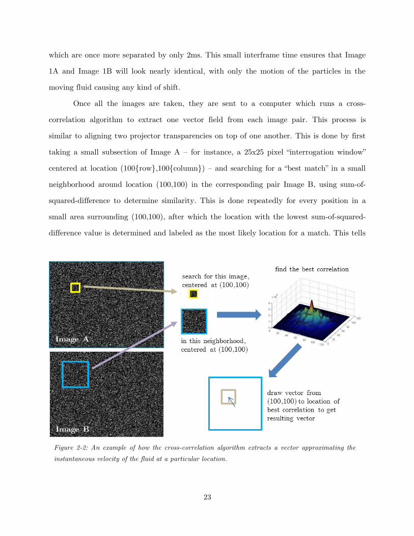
Once all the images are taken, they are sent to a computer which runs a cross-

correlation algorithm to extract one vector field from each image pair. This process is

similar to aligning two projector transparencies on top of one another. This is done by first

taking a small subsection of Image A – for instance, a 25x25 pixel “interrogation window”

centered at location (100{row},100{column}) – and searching for a “best match” in a small

neighborhood around location (100,100) in the corresponding pair Image B, using sum-of-

squared-difference to determine similarity. This is done repeatedly for every position in a

small area surrounding (100,100), after which the location with the lowest sum-of-squared-

difference value is determined and labeled as the most likely location for a match. This tells

Figure 2-2: An example of how the cross-correlation algorithm extracts a vector approximating the

instantaneous velocity of the fluid at a particular location.

24

us where the particles we saw in the 25x25 pixel “interrogation window” from Image A have

most likely traveled to by the time Image B was taken. This allows us to draw a vector

from the center of the window in Image A (100,100) to the location of the best match in

Image B - for instance (97,97) – meaning that the particles imaged in that section moved

roughly 3 pixels up and 3 pixels to the left during the interframe time.

If we do this repeatedly, hundreds of times, over the entire image, with our

“interrogation window” locations aligned in a 30x30 grid, we can develop a vector field

describing the approximate direction of fluid flow over the camera’s field of view. From

there, many other interesting things can be done, such as calculating vorticity, and

observing flow structures and their evolution over time.

2.2 Real-time PIV

As useful as PIV is, it has the capability to do more, and expand its role in the research

world. Currently, PIV is done in two stages: first, the experiment is set up and the images

captured; second, the images post-processed and analyzed using the cross-correlation

approach. This approach is largely free from any kind of temporal restrictions, and a high

degree of manual input can be used to ensure the best possible results. For instance,

researchers can continually adjust various parameters, such as the size of the interrogation

windows, the spread of the “neighborhood” in which to search for the best match, the

number of vectors calculated for each image pair, and so on. Indeed, more sophisticated

cross-correlation algorithms can be used that result in fewer errors in the resulting vector

field. While this means that a great amount of effort can be done towards analysis, it also

means that the PIV results cannot be used to influence the experiment in real-time. This

may be perfectly acceptable for someone seeking to simply observe fluid flow phenomena,

but it also means that PIV remains unappealing to other areas of study.

25

However, if it were possible to increase the efficiency of this process and develop a

method that could perform PIV from a live video stream in a very short time scale and

obtain results in real time, it would open up a whole new realm of experimental possibilities.

Researchers could change experiment conditions on the fly and see their repercussions in as

they happen, or even use the vector field result as part of an autonomous feedback loop in

experiments. Essentially, instead of forcing researchers take pictures of this invisible world

of fluid dynamics and study them after the fact, we would be giving them a proverbial

magical lens that could reveal the complex motions of the fluid in real time.

Fortunately, research into this possibility has just begun to appear, thanks to some

very recent work done by several research groups. Most of these approaches utilize a Field

Programmable Gate Array (FPGA) to create a fast, custom architecture for PIV analysis.

This is a promising approach that has potential for high throughput from a compact,

relatively inexpensive device.

Even at this early stage, real-time PIV is demonstrating its versatility and exciting

new possibilities. Last year, Dr. John Roberts, my undergraduate thesis advisor and fellow

researcher at MIT CSAIL’s Robot Locomotion Group was able to use an off-the-shelf

commercial GPU to perform real-time PIV as part of his PhD thesis “Control of

underactuated fluid-body systems with real-time particle image velocimetry”. Yet more

importantly, he was able to use the result as part of a feedback loop in a control task. This

task sought to “balance” a flat plate connected by a hinge to a motorized “cart” against the

a laminar flow in a water tunnel, fighting weathercock stability by moving the “cart” along

a track perpendicular to the flow of the water. It was dubbed the “hydrodynamic cart-pole”

problem due to its similarity to the traditional cart-pole problem found in control theory.

His research showed that not only is there great potential to do smarter control

underwater, but that knowledge of the fluid state, revealed through the real-time PIV, did

indeed improve performance of the task, tantalizingly opening the door for further research

26

into methods to illuminate fluid state for the sake of improving locomotive efficiency and

control authority.

My own undergraduate thesis built off of these experiments, and demonstrated

another interesting use of real-time PIV – the ability to potentially identify periodic flow

structures and even predict obstructions upstream by analyzing the real-time vector fields

generated by the PIV algorithm.

Real-time PIV is beginning to change what is possible with the traditional PIV

technique, and is giving a powerful new tool to many fields of research that may otherwise

have never used it. It may help us dramatically improve the efficiency and accuracy of robot

locomotion in the air and underwater, help find new ways to efficiently manage wind farms,

allow researchers to gain a better understanding of how fluids move in the human body,

enable the creation of better aircraft, and much more. It is a way to illuminate an otherwise

invisible medium that is extraordinarily difficult to model, and do so in such a way that we

can see what is happening as it happens, and use that information in novel ways.

2.3 M otivation and Goals

While real-time PIV as opened up an exciting new chapter in the technique’s history, it has

also revealed some new issues that did not exist before. With normal PIV, there were no

time restrictions due to the fact that calculations were done after the images were taken,

and vector fields could be created with as much manual input as was necessary, from

deliberately fixing stray vectors to adjusting PIV settings such as interrogation window size,

and even the cross-correlation algorithm itself to achieve a near-perfect result.

However, when dealing with real-time PIV, most of these steps become luxuries, due

to the fact that the calculations must be done on a sub-second timescale. This means that

there is little to no opportunity for manual input, and the algorithm is on its own once the

camera starts rolling. While it is true that these attributes can be set beforehand, as the

27

flow conditions change, so do the optimal PIV settings. If the flow increases or decreases in

speed in different areas, the PIV algorithm must be adjusted, or if the density of the

reflective seeding particles changes. A standard “one size fits all” approach only works so

well when the images being analyzed are changing rapidly, and exhibit wholly different

characteristics not only over a period of time, but within the same field of view in a single

image.

As such, it is necessary to develop a way to counteract these effects and ensure that

the accuracy of the result is as high as possible. In short, there are three main issues with

real-time PIV that uses a normal, grid-like approach:

Accuracy: With different characteristics in different parts of the image – for

instance, varying densities of the reflective seeding particles, and changing

velocity magnitudes – there are different ways a PIV algorithm should handle

these parts. Finding an algorithm that accurately accounts for these

differences is key.

Efficiency: The number of cross-correlations that are done within a single

image for traditional PIV is staggering. However, it may be possible, with

smarter analysis, to reduce that number and focus on the areas of the image

where the most relevant fluid structure information is held.

Adaptability: Another very important issue that must be fixed is that the

new PIV algorithm must be able to automatically adapt to changes in flow

conditions with minimal human intervention. The time scales in which the

PIV calculations must be completed are far too short for any manual review

of the results, so any error-corrections, adaptations, or other features must be

able to run without much hand-holding.

28

This new, smarter, real-time particle image velocimetry has the potential to improve the

emerging field of real-time PIV with specific modifications to help it improve in these three

key areas. One fantastic starting point for such an approach would be by looking at another

very new sub-field of PIV – adaptive PIV. There is limited but visible work being done to

develop and apply techniques that evaluate the different properties within a PIV image,

such as seeding particle density, and create a more accurate vector field representation of

the fluid flow. However, the approaches detailed in these works are, once again, for non-

real-time settings, and significant adaptations will have to be made to combine these

adaptive PIV techniques to the real-time PIV setting.

2.4 Related W orks

There are two major fields of PIV research that will be relevant to the work outlined in this

paper – one that deals with the emerging technology of real-time PIV systems, and one that

deals with a novel techniques being proposed in adaptive PIV methods.

2.4.1 Works on Related Real-Time PIV

As stated before, there has been research work from several groups detailing proposals for

real-time PIV systems. The first such implementation was 1997 by Carr et al. who

developed a digital PIV technique that ran in a very small interrogation area. From there,

FPGA-based methods became common, with Maruyama et al. publishing such an

implementation in 2003. Their method used an off-the shelf Virtex-II FPGA to perform

calculations specific to a particular interrogation region size. French researchers Fresse et al.

published a similar system in 2006. That same year, Tadmor et al. from Northeastern

University in Boston published another FPGA-based method that used reconfigurable

29

architecture that allowed for real-time PIV analysis that was independent of the design

specifics of the PIV system, such as interrogation region size.

Non-FPGA work with real-time PIV is even more difficult to come by – with only

two main works of note being published in the last 3 years. The first is from California

Institute of Technology, from Gharib et al. who used a standard dual-core PC system, with

no parallel architecture in their approach. The second work was accomplished in 2012 by

the aforementioned Dr. John Roberts of MIT, my undergraduate research advisor, who was

able to leverage the power of parallel processing offered by off-the-shelf GPUs using CUDA.

His approach was unique, as he was able to utilize the result as part of a feedback loop in a

hydrodynamic controls problem, directly demonstrating PIV’s potential usefulness to the

field of control theory and robotics. It is on his work that much of the research outlined in

this paper is based.

2.4.2 Works on Related Adaptive PIV

The adaptive side of my approach draws upon works done by several research groups to

utilize various cross-correlation settings for PIV analysis of a single image. This general idea

has been around for over a decade, with Riethmuller et al. proposing in 2000 to

progressively redefining window size with iterative interrogation steps to improve accuracy

and resolution. Other algorithms emerged that began to rely on various characteristics of

the image to define window size. Scarano et al. in 2002 utilized local velocity fluctuations to

do so, and Susset et al. used signal-to-noise ratio to do the same in 2004.

However, my approach is adapted from that of Theunissen, Scarano, and

Riethmuller from 2007, who combined local velocity fluctuations with seeding particle

density to reach a metric that would define window size and the number of vectors analyzed

in a particular area.

All the methods mentioned in this section deal with off-line methods for achieving

improved accuracy with adaptive PIV. However, these same methods can offer a lot to the

30

burgeoning field of real-time PIV, and that in fact, real-time PIV truly needs adaptive

techniques in order to become a reliable and accurate research tool. This paper seeks to do

exactly this – to join a real-time PIV implementation with adaptive PIV techniques in order

to create a powerful technique that can reveal the invisible subtleties of complex fluid flow

as they occur.

31

Chapter 3

Hardware and Experimental

Setup

3.1 Hardware Used

There was extensive hardware used in this research, with some of it custom-built, and

others using commercial components.

3.1.1 Water Tunnel

The water tunnel used in these experiments was built by Steven Proulx (a former member

of the lab staff), and John Roberts. It was designed for the purposes of studying fluid-body

system interactions within a controlled environment. It features two stainless-steel pumps

which feed water to a settling tank, which then flows through flow straighteners (a set of

small-diameter tubes arranged in a honeycomb pattern), and then a contraction section,

before reaching the test section, and after that, returns to the pumps to be recirculated.

32

The important things to note for this experiment are that it offers a very controlled,

laminar flow in the test section – a perfect setup for PIV research. Objects can be placed

upstream of the test section, as well, providing interesting wakes and fluid flow structures

to analyze. Additionally, flow can be stopped until the water reaches a standstill, if more

subtle experiments involving slower flows are desired. In my experiments, only one pump

was utilized to circulate the water, which led to a flow speed of roughly 11 cm/s.

3.1.2 Laser and Optics

For the laser used in the experiments, a LaVision 2 Watt Continuous Wave laser was used

which emitted a green beam of wavelength 532nm, matching the high quantum efficiency

wavelength range of our camera. This laser was not as strong as many of the lasers used in

high-speed PIV setups, but was able to perform at an adequate level for the experiments

detailed in this paper. John Roberts was able to use a very powerful 100mJ double-pulsed

laser in his experiments, which enabled him to run both pumps, making the flow speed

roughly 22 cm/s. Due to the nature of the laser, enough light could be outputted within the

Figure 3-1: Left: A picture of the water tunnel setup used. Right: A schematic showing the flow of

water through the system.

33

short time that the camera shutter was open so that a clear, well-lit, blur-free image could

be taken, even at those high speeds. With a less powerful laser, the experiments were

restricted to slower speeds in order to ensure no significant motion blur occurred.

The beam was split into a 2D laser sheet by a cylindrical lens (ThorLabs anti-

reflectivity coated cylindrical lens with a focal length of -38.1mm, part number LK1325L1-

A). This lens was mounted to the laser itself, ensuring there would be minimal problems

with alignment.

The room windows and sections of the water tunnel itself were covered in opaque

black tarp as a safety precaution, and protective eyewear was used whenever the laser was

on.

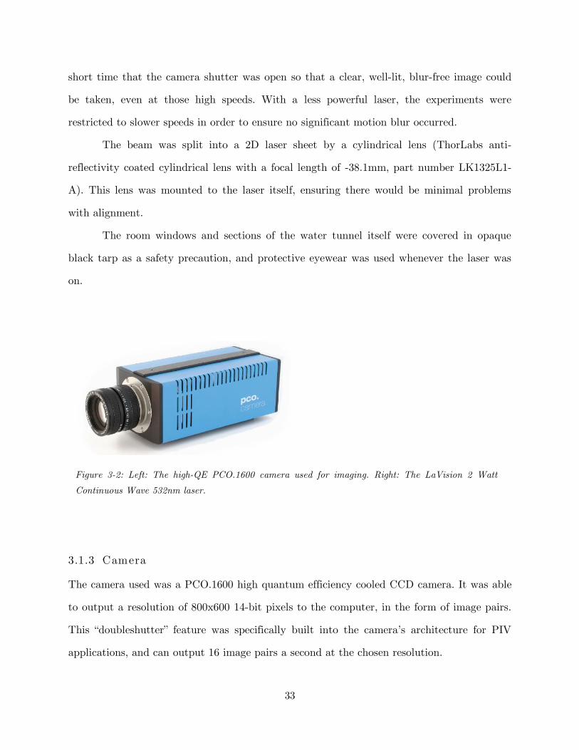
3.1.3 Camera

The camera used was a PCO.1600 high quantum efficiency cooled CCD camera. It was able

to output a resolution of 800x600 14-bit pixels to the computer, in the form of image pairs.

This “doubleshutter” feature was specifically built into the camera’s architecture for PIV

applications, and can output 16 image pairs a second at the chosen resolution.

Figure 3-2: Left: The high-QE PCO.1600 camera used for imaging. Right: The LaVision 2 Watt

Continuous Wave 532nm laser.

34

The camera was placed underneath the test section, looking up through a

transparent piece of plastic making up the floor of that segment. The magnification is such

that one pixel represents 0.158mm. In order to protect the camera from water leakage, it is

housed in an aluminum mounting box, with a clear glass ceiling designed by John Roberts.

The camera is screwed in place rigidly to the inside wall of the box, facing upwards in order

to see into the test section.

3.1.4 Seeding Particles

The particles used in these experiments were 50µm polymer particles made specifically for

PIV application by Dantec Dynamics (part number PSP-50). After mixing via the water

pumps, the particles remain suspended in the water, being roughly neutrally buoyant.

The size and type of the particles was chosen specifically to provide enough scattered

light from the laser sheet to produce a clear image from the camera.

3.1.5 Computer Hardware

There were two computers used in the experiments, both standard dual-core machines. The

camera computer, however, featured an NVidia GeForce GTX 570 with 480 unique cores,

which was used to run the parallelized CUDA code that performed the cross-correlations.

The camera sent data directly to the computer, which was able to process the information

in real time using the PIV algorithm, and send the results to the second computer via

Lightweight Communications and Marshalling protocol (LCM) developed by the MIT

DARPA Urban Challenge Team in 2008.

The visualization computer ran a MATLAB script that read the LCM stream from

the camera computer over the local area network and displayed the calculated vector field

in real time.

3.1.6 Arduino

35

To convert the continuous wave laser into a pulsed laser suitable for the doubleshutter

camera, some work was necessary to ensure the timings synced up perfectly. An off-the-shelf

Arduino Uno was used to ensure that this was done properly (detailed in 3.2).

3.2 Implementing the Basic PIV Setup

There was a unique challenging in converting the continuous wave laser into a laser suitable

for PIV application. Traditionally, powerful double-pulsed lasers are used to allow for

lighting during the capture of the image pairs, but in the absence of such hardware, another

way had to modulate the laser output so that it lined up with the camera shutter, while still

producing enough light to capture a clear image.

This challenge stems from a trait of the doubleshutter mode of the PCO.1600

camera. While Image A can be finely controlled by the user in terms of exposure time, the

corresponding image pair cannot. After a short, non-modifiable interframe time after the

capture of Image A, the camera begins to capture Image B for a period of time that cannot

be manually set. This second exposure time tends to be much longer than the exposure time

of Image A, meaning that the resulting image exhibits far more motion blur than Image A.

Since PIV is built upon comparing minute differences between Image A and Image B, it is

of utmost importance that the two images are similar in every way, in terms of exposure,

contrast, and other such metrics, and only differ in the small changes in the positions of

illuminated seeding particles.

The LaVision 2 Watt laser has an input for a TTL signal that can modulate the

laser output, meaning that if one cannot command the camera shutter to be open for a set

amount of time during Image B, it might be possible to command the laser light to only be

on for that desired length of time, to match the exposure characteristics of Image A. An

example signal that could accomplish such a goal might behave as follows:

36

On for the entirety of the capture of Image A. Since it is possible to strictly

define the exposure time for Image A, no special illumination steps have to be

taken.

Off for a set amount of time after Image A. This time would be the desired

interframe time between Image A and Image B. The camera shutter may

open for the capture of Image B during this time, but as there is no light to

illuminate the scene, no stray image information would be captured.

On for a set amount of time to capture Image B. While the camera shutter

remains open for an extended period of time for Image B, it would be possible

to only illuminate the scene with the laser for a short period of time, so that

we attain an image that is similar to Image A.

For example, if the desired exposure time of each image in the pair is 8ms, and we desire an

interframe time of 3 ms, then we would set Image A to be exposed for 8ms. We would turn

the laser on for the entirety of Image A’s capture, after which time we would modulate the

laser signal to be off for 3ms, and then on for another 8ms while the camera shutter is open

for Image B. This would result in an Image A that had been exposed for a total of 8ms, and

an Image B that had been exposed for a total of 8ms, starting 3ms after the end of Image

A.

Since the camera shutter is open for a significant period of time for the capture of

Image B, we have a significant amount of freedom in deciding how much interframe time

and exposure time to use.

I decided to use a simple Arduino Uno for this procedure, and began by using a

software-based trigger to modulate the laser. Every time the program loop requested an

image from the camera, it would send a signal to the Arduino to begin a sequence of on/off

signals that would produce the desired exposures for Image A and B. However, this

approach was not fruitful, as there were inherent delays in the system.

37

Instead, a feature of the PCO.1600 camera hardware was utilized that outputted a

“high” signal via BNC while Image A was being captured. This signal was fed into the

Arduino, which would replicate the input signal and send it to the laser, with the added

feature that when it detected a transition from “high” to “low” (signaling the end of the

Image A capture), it ignore incoming information for a time while it outputted a “low” for

the desired interframe time, followed by a “high” pulse for the Image B exposure time.

This approach worked very well, leading to image pairs that were nearly identical in

the way they looked. After some experimentation with exposure times, a suitable setting

was found where there was enough light for the camera to capture a clear, if somewhat dim,

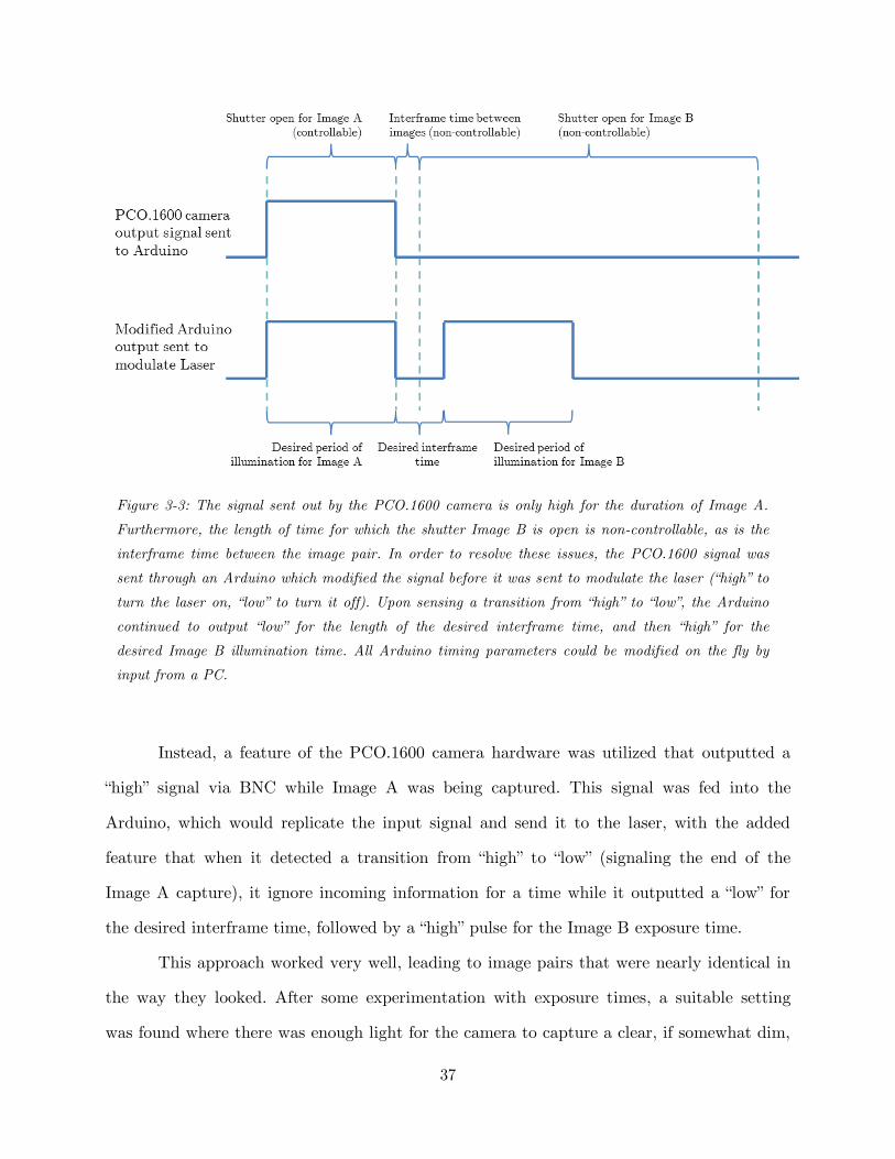
Figure 3-3: The signal sent out by the PCO.1600 camera is only high for the duration of Image A.

Furthermore, the length of time for which the shutter Image B is open is non-controllable, as is the

interframe time between the image pair. In order to resolve these issues, the PCO.1600 signal was

sent through an Arduino which modified the signal before it was sent to modulate the laser (“high” to

turn the laser on, “low” to turn it off). Upon sensing a transition from “high” to “low”, the Arduino

continued to output “low” for the length of the desired interframe time, and then “high” for the

desired Image B illumination time. All Arduino timing parameters could be modified on the fly by

input from a PC.

38

image, with minimal motion blur. To improve the image quality, a final postprocessing step

was added that manually bumped up the contrast so that the seeding particles could be

clearly distinguished from the dark background.

39

Chapter 4

The DARTPIV Algorithm

4.1 Theory and Approach

To develop an approach that could take techniques from adaptive PIV and apply them in a

real-time PIV context, there were several things to consider.

First, the steps followed in adaptive PIV had to be made more efficient, so as

to be completed in a very short time scale over a relatively large image of

800x600 pixels.

Second, the algorithm still had to be parallelizable, even after using different

window sizes and other such steps, and be able to use much of the CUDA

architecture already in place.

Third, it had to be able to work for a variety of flow conditions, and change

between them on the fly, without any intervention from the user. While the

adaptive approach would allow for variations in a single image to be

accounted for, there is nothing in the PIV algorithm that accounts for major

40

changes in flow conditions over time – for instance, if the flow speed increases

or decreases dramatically, or a solid body in the test section is removed or its

shape changed (for instance, a robotic fish).

The output had to still be a vector field – that is, an ordered grid of vectors.

This would make it easy to do further analysis on vorticity, and other such

calculations, if desired.

A starting point for the approach began with the methodology outlined by Theunissen,

Scarano, and Riethmuller in 2007. They point out that in areas where there is increased

seeding particle density, smaller interrogation windows can be used, and in fact, will lead to

more accurate results. However, in order to compensate for the reduced coverage, more

interrogation windows will need to be looked at in those regions. Similarly, when there is a

large local variation in velocity, smaller interrogation windows are needed in order to reduce

the chance of selecting a window in which particles are moving in multiple directions, which

would result in a faulty vector being generated. But again, the number of interrogation

windows would have to increase in order to capture the different sets of velocity vectors

packed into that small area.

Essentially, as particle density and local velocity variation increase, interrogation

windows in that area should decrease in size but increase in number. This was the essence

of their approach which was carried into the present real-time implementation. An

additional step that was included to make the system more dynamic and robust to

variations over time was to make use of the ability to set the interframe time on the fly

through the Arduino. This Dynamic feature of the Adaptive, Real-Time PIV system is the

motivation behind the acronym DARTPIV.

4.1.1 Seeding Particle Density

41

To implement the adaptive PIV algorithm, a computationally efficient way of evaluating

seeding particle density over the 800x600 pixel image had to be developed. Given the real-

time nature of my application, simply attaining an approximation of this factor would be

sufficient.

The approach of Riethmuller et al. utilized a technique used in Particle Tracking

Velocimetry (PTV) to individually count the number of particles in selected areas – a

process that involves background subtraction and intensity thresholding, which would have

been too computationally expensive for a real-time approach. Instead, a “sliding window”

approach to calculate local average pixel intensity. For instance, when evaluating the

seeding particle density of location (100,100), all pixels in a 25x25 pixel box around that

location would be taken and values averaged. Since each seeding particle is roughly the

same size, and shows up as small white group of high-valued pixels, a greater average value

within a window would mean there were more seeding particles in that region.

This approach is easy to implement, is reasonably accurate, and can be implemented

relatively efficiently by leveraging the high amount of overlap in the sliding window

approach.

4.1.2 Local Velocity Variation

The strategy for efficiently obtaining local velocity variation information also relied upon

finding a shortcut of sorts in order to obtain a reasonable estimate, as opposed to placing

emphasis solely on accuracy.

The unique challenge about this step, however, is that in order to determine local

velocity variations in a particular image, a vector field must already be in place. That is, in

order to do PIV that takes into account local velocity variations, we must already have PIV

completed. However, since this was a system where image pairs are separated only by a

fraction of a second, it would be reasonable to assume that the vector field calculated from

the previous image pair would still do a good job roughly describing the vector field in the

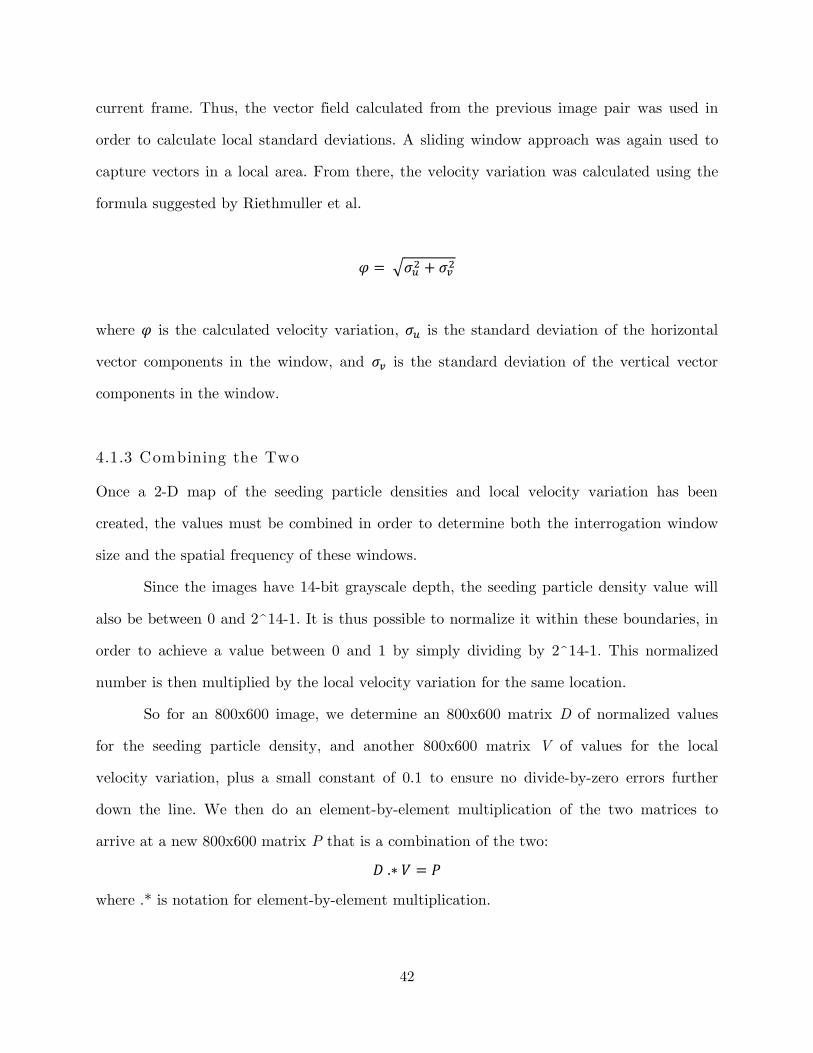
42

current frame. Thus, the vector field calculated from the previous image pair was used in

order to calculate local standard deviations. A sliding window approach was again used to

capture vectors in a local area. From there, the velocity variation was calculated using the

formula suggested by Riethmuller et al.

√

where is the calculated velocity variation, is the standard deviation of the horizontal

vector components in the window, and is the standard deviation of the vertical vector

components in the window.

4.1.3 Combining the Two

Once a 2-D map of the seeding particle densities and local velocity variation has been

created, the values must be combined in order to determine both the interrogation window

size and the spatial frequency of these windows.

Since the images have 14-bit grayscale depth, the seeding particle density value will

also be between 0 and 2^14-1. It is thus possible to normalize it within these boundaries, in

order to achieve a value between 0 and 1 by simply dividing by 2^14-1. This normalized

number is then multiplied by the local velocity variation for the same location.

So for an 800x600 image, we determine an 800x600 matrix D of normalized values

for the seeding particle density, and another 800x600 matrix V of values for the local

velocity variation, plus a small constant of 0.1 to ensure no divide-by-zero errors further

down the line. We then do an element-by-element multiplication of the two matrices to

arrive at a new 800x600 matrix P that is a combination of the two:

where .* is notation for element-by-element multiplication.

43

4.1.4 Spatial Frequency of Interrogation W indows

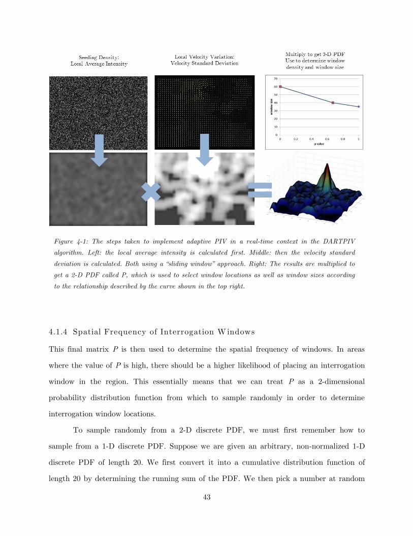
This final matrix P is then used to determine the spatial frequency of windows. In areas

where the value of P is high, there should be a higher likelihood of placing an interrogation

window in the region. This essentially means that we can treat P as a 2-dimensional

probability distribution function from which to sample randomly in order to determine

interrogation window locations.

To sample randomly from a 2-D discrete PDF, we must first remember how to

sample from a 1-D discrete PDF. Suppose we are given an arbitrary, non-normalized 1-D

discrete PDF of length 20. We first convert it into a cumulative distribution function of

length 20 by determining the running sum of the PDF. We then pick a number at random

Figure 4-1: The steps taken to implement adaptive PIV in a real-time context in the DARTPIV

algorithm. Left: the local average intensity is calculated first. Middle: then the velocity standard

deviation is calculated. Both using a “sliding window” approach. Right: The results are multiplied to

get a 2-D PDF called P, which is used to select window locations as well as window sizes according

to the relationship described by the curve shown in the top right.

44

between the minimum (first) and maximum (last) values of the CDF, and begin to step

through each of the 20 values in order. Once we reach a number that is greater than or

equal to our previously determined random number, we take the index of that number as

our answer.

To expand this into a 2-D setting, suppose we have a 30x20 matrix that we wish to

sample from as a 2-D discrete PDF. The first step is to sum the values within each of the 20

columns so that we obtain a 1-D row of 20 numbers. We then apply the familiar 1-D

discrete PDF selection algorithm to this row in order to select an index, called c. We then

consider the column from the original 30x20 matrix, and once more apply the 1-D

discrete PDF problem to select an index, called r. This leaves us with our result, in the

form of (r,c).

For the DARTPIV approach, we repeat this process once for every vector we wish to

analyze – that is, if we want to extract 700 vectors from an image, we would repeat this

process 700 times. For computational efficiency, we calculate the column-sum CDF and

each of the individual column CDFs once, and store them (since the total number of vectors

we want to analyze is typically greater than the number of columns, or width, of the image,

it is generally more efficient to simply pre-calculate CDFs for each column and refer back to

them instead of calculating a new column CDF for each vector).

4.1.5 Interrogation W indow Sizes

Once a location has been selected for the interrogation window from the 2-D discrete PDF

P, the size of the interrogation window must be determined. This means finding a way to

translate the value of P at the selected point into a size for the interrogation window. Since

P is a value that increases as seeding density and local velocity variation increase, this

means that for large values of P, we want small interrogation window sizes, and vice-versa.

But determining precisely what those sizes will be is its own challenge.

45

This investigation began by creating some simulated PIV images using a MATLAB

script that would position white dots resembling illuminated seeding particles upon a black

background, and create a second image in which the dots had moved according to a set

pattern – namely, that of a smoothed Rankine vortex model. The use of simulated images

meant that the “true” vector field for the image pair was known, and could be used as a

baseline ground truth. The simulated images that were used included a wide range of values

for P for testing.

Another MATLAB script that performed normal PIV was then used. The algorithm

was run many times, with small increments in the size of the interrogation windows upon

every iteration. Thus, at the end of the process, a set of vector fields from many different

interrogation window sizes was created. Each one of these vector fields was then compared

to the “ground truth” vector field. If a vector field created by a window size of 25 pixels was

able to attain results similar to the “ground truth” with little error in areas where the value

of P ranged from, for instance, 0.2 to 0.4, then it could be concluded that for those P

values, a window size of 25 pixels would be appropriate.

Conducting this analysis over the entire range of vector fields allowed for an

approximate function to be created, whereby an input P value could be transformed into an

output value that described the optimum window size. Of course, it was possible for several

window sizes to come up with good results for the same values of P, so some liberty was

taken to ensure the curve was smooth, while still staying within the bounds of the optimal

window sizes.

Of course, there is no guarantee that this same curve will be optimal for all PIV

setups. If the camera has a different focal length or the size of the seeding particles is

different, a new curve will have to be made following the same methodology.

4.1.6 Cross-Correlation

46

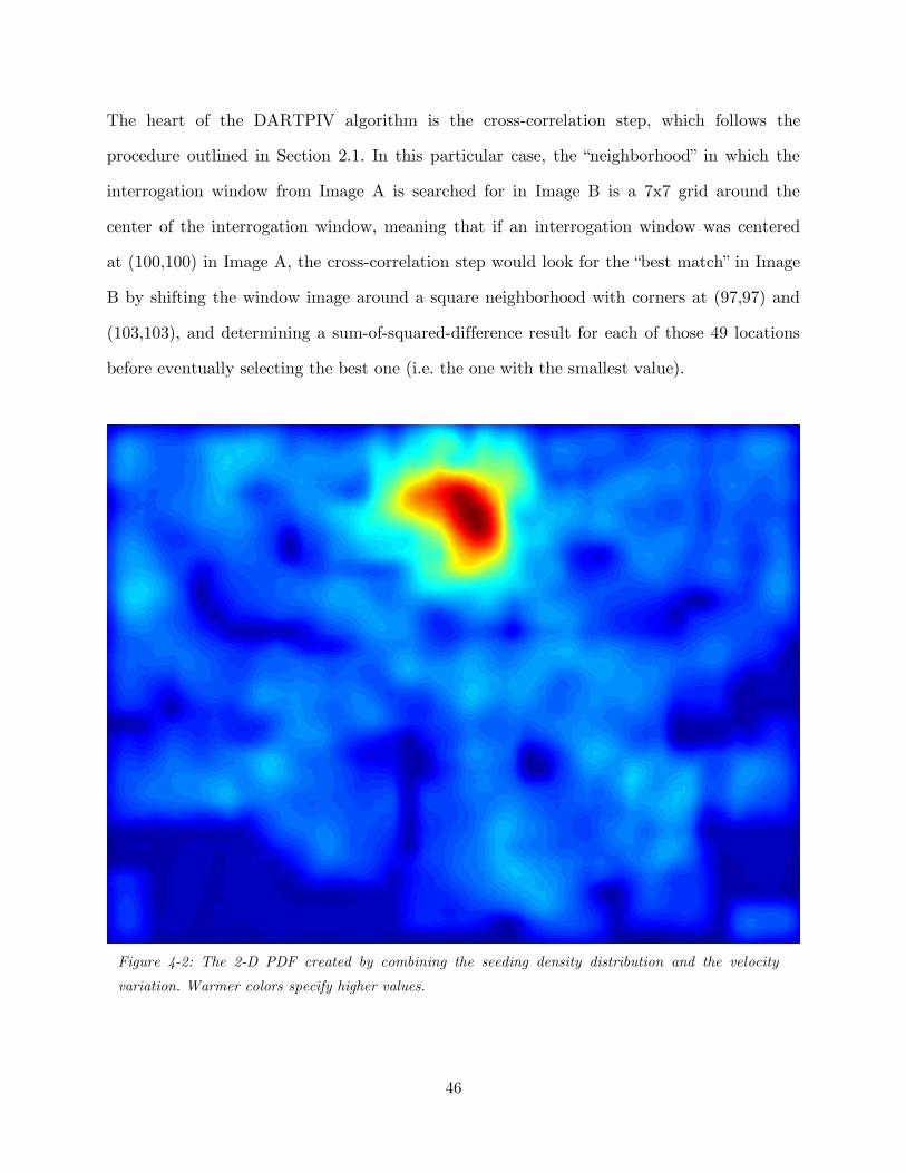
The heart of the DARTPIV algorithm is the cross-correlation step, which follows the

procedure outlined in Section 2.1. In this particular case, the “neighborhood” in which the

interrogation window from Image A is searched for in Image B is a 7x7 grid around the

center of the interrogation window, meaning that if an interrogation window was centered

at (100,100) in Image A, the cross-correlation step would look for the “best match” in Image

B by shifting the window image around a square neighborhood with corners at (97,97) and

(103,103), and determining a sum-of-squared-difference result for each of those 49 locations

before eventually selecting the best one (i.e. the one with the smallest value).

Figure 4-2: The 2-D PDF created by combining the seeding density distribution and the velocity

variation. Warmer colors specify higher values.

47

The particular cross-correlation approach outlined here is called direct cross-correlation.

Other methods exist as well, including those which use fast Fourier transforms to extract a

vector. However, direct cross-correlation was used in this case due to its simplicity and

parallelizability.

4.1.6 “Gridify”-ing and Dynamic Interframe Time Adjustment

The final step of the algorithm is to “gridify” the results – that is, to convert a set of vectors

arranged with no particular alignment over the image into an ordered grid of vectors

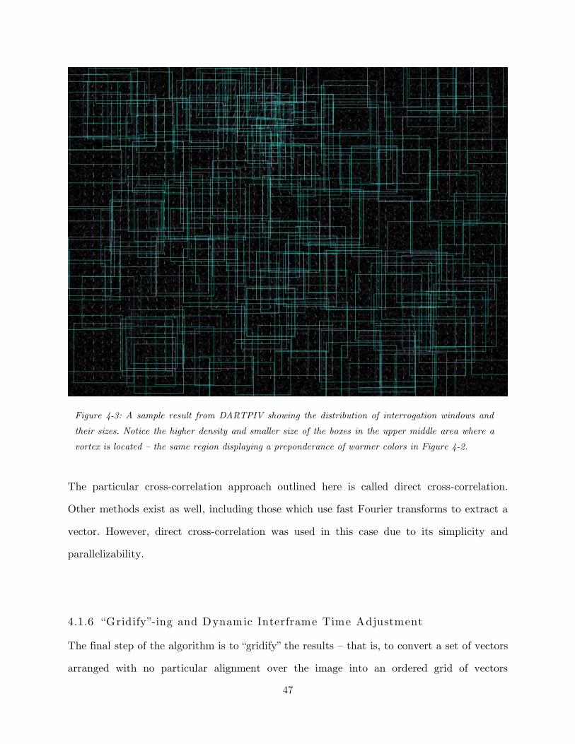
Figure 4-3: A sample result from DARTPIV showing the distribution of interrogation windows and

their sizes. Notice the higher density and smaller size of the boxes in the upper middle area where a

vortex is located – the same region displaying a preponderance of warmer colors in Figure 4-2.

48

comprising a vector field. This was a fairly simple operation – for each point in the grid, the

algorithm searched for the two closest evaluated vectors determined by Euclidian distance

to their origin (i.e. the center of their respective interrogation windows), and performed a

weighted average to determine the final product. This calculated value represents the

predicted displacement of the fluid in that interrogation window.

While this calculation is being done, the algorithm also keeps track of these

displacement magnitudes. Since we are searching in a 7x7 grid during the cross-correlation

step in this PIV algorithm, the largest displacement vector that can be produced is

<±3,±3>. This means that the largest shift in seeding particles that we can reliably detect

between image pairs is roughly 3 pixels. If the flow is faster, the displacements will be

greater than this amount, and errors will accumulate. Similarly, if the flow is slower,

displacements may be so small between frames that the algorithm simply finds vectors of

zero magnitude. Thus, it is worthwhile to attempt to ensure that the majority of the

displacements (that is, the average magnitude of the vectors) fall between 0 and 3. Since we

have control over the interframe time thanks to the Arudino Uno that is modulating the

laser, it is possible to work towards this goal.

Thus, as the values are being written to the vector field grid, two more subtle yet

important things are being done:

First, the average displacement magnitude is being calculated. If this number

is above 1.5, the interframe time decreased proportionally. For instance, if the

interframe time is 6ms and the average vector magnitude is 3, then the

algorithm is pushing the boundaries of what it can detec, and the interframe

time should ideally be shifted back down. Adjusting it such that it is 3ms

instead of 6ms would cause the average displacement magnitude to decrease

into a more appropriate range, as well. A simple proportial-difference

approach was taken here, whereby difference between the average

displacement magnitude and the desired 1.5 pixels was multiplied by a

49

constant factor and added or subtracted as necessary from the interframe

time on the fly.

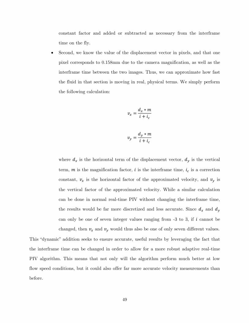
Second, we know the value of the displacement vector in pixels, and that one

pixel corresponds to 0.158mm due to the camera magnification, as well as the

interframe time between the two images. Thus, we can approximate how fast

the fluid in that section is moving in real, physical terms. We simply perform

the following calculation:

where is the horizontal term of the displacement vector, is the vertical

term, is the magnification factor, is the interframe time, is a correction

constant, is the horizontal factor of the approximated velocity, and is

the vertical factor of the approximated velocity. While a similar calculation

can be done in normal real-time PIV without changing the interframe time,

the results would be far more discretized and less accurate. Since and

can only be one of seven integer values ranging from -3 to 3, if cannot be

changed, then and would thus also be one of only seven different values.

This “dynamic” addition seeks to ensure accurate, useful results by leveraging the fact that

the interframe time can be changed in order to allow for a more robust adaptive real-time

PIV algorithm. This means that not only will the algorithm perform much better at low

flow speed conditions, but it could also offer far more accurate velocity measurements than

before.

50

4.2 Implementation Details

The DARTPIV algorithm was implemented twice – first in MATLAB, as a proof of concept

to test out the theory; and second, in C++/CUDA for the actual real-time implementation.

4.2.1 M ATLAB Proof-Of-Concept

The MATLAB implementation was an initial test run to serve as a guinea pig for

implementing a quick-and-dirty version of the adaptive PIV algorithm. It used the same

approach as outlined in Section 4.1, but without any emphasis on parallel processing. Use of

MATLAB’s built-in functions and various visualization tools made it a fantastic initial

prototyping tool, and helped set the stage for the C++/CUDA implementation later on.

4.2.2 C++/CUDA Implementation

The real implementation came after the MATLAB proof-of-concept was tried and tested.

Building off of John Robert’s real-time PIV code, the DARTPIV algorithm was carefully

adapted to the real-time context.

The code implementation here as well followed the sequence laid out in Section 4.1.

One major difference, however, was the implementation of the parallel processing step in the

cross-correlation section. When creating a CUDA-based algorithm, several constraints must

be satisfied:

1. Since all calculations are performed in parallel, as opposed to sequentially,

any calculations performed cannot depend on the results of a previous

calculation. For instance, in a “for” loop, one can save variables from the

previous iteration of the loop for use in the next iteration. However, with

CUDA, all such information must be pre-processed.

51

2. The CUDA memory architecture is separate from that of the computer, and

as such all relevant variables must be allocated for in CUDA memory and

transferred before the parallel processing step can take place.

When implementing normal PIV, this is not much of a hassle – interrogation window sizes

are constant, and window locations follow a simple, evenly-spaced vector field grid.

However, with an adaptive approach, each set of cross-correlations for a specific window will

has its own window size and window location. These are not constants, nor can they

described by a simple linear equation, and as such they must be transferred into CUDA

memory before the parallel processing step. Here, too, there is a challenge: it is not easy to

transfer thousands of separate variables to CUDA memory many times every second. As a

result, they are stored as long arrays, and require clever indexing in order to be accessed

properly by each individual CUDA thread.

To resolve this issue, the DARTPIV approach sends several arrays to the CUDA

memory: an array that contains pixel values for all the interrogation windows from Image A

(arranged sequentially), an array that contains a list that details the index at which each

window starts in the first array, an array that lists window sizes, an array that lists window

locations, and an array containing all pixels in Image B. Each thread can reference its own

thread number to determine where to index each one of these arrays.

Each thread in the CUDA implementation is responsible for all cross-correlations

corresponding to one interrogation window. Thus, even if there are enough threads to

perform analysis of all interrogation windows simultaneously, the program would still have

to wait for all of them to finish before proceeding. The limiting factor, then would be

whichever of those threads has the most work to do – likely the thread with the largest

interrogation window size. However, it is important to note that the cross-correlation step is

only one of many steps in the adaptive PIV sequence. In fact, in practice, reducing the size

of the interrogation windows only provided incremental benefits to speed, while negatively

impacting accuracy.

52

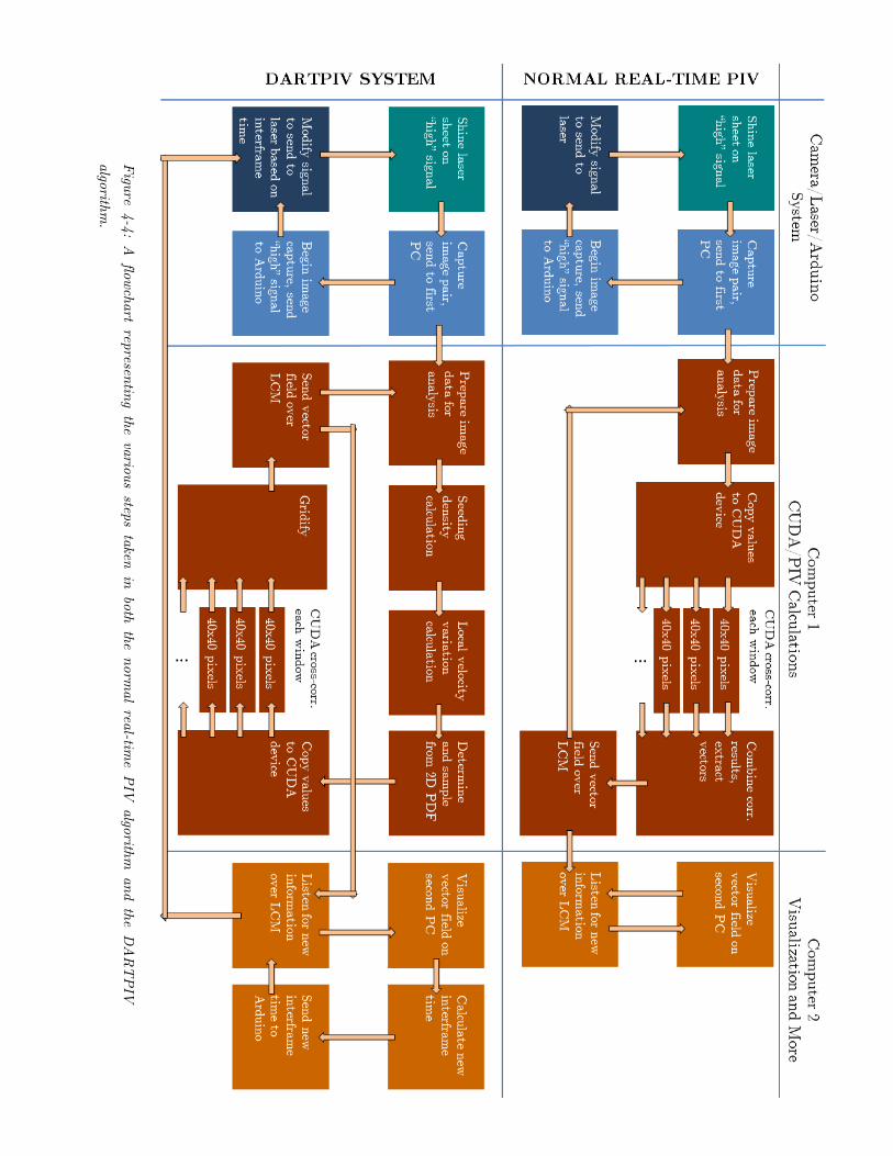
Figu

re 4-4

: A

flo

wch

art

represen

ting

the

vario

us

steps

taken

in

bo

th th

e norm

al

real-tim

e PIV

algo

rithm

and th

e D

AR

TPIV

algo

rithm

.

53

Chapter 5

Experiments, Results, and

Discussion

5.1 Experimental Approach

In order to demonstrate the unique advantages afforded by the DARTPIV algorithm, it was

necessary to devise a set of experiments that would not only put it to the test against

alternative approaches, but also do so in an objective, rigorous manner. The proposed

advantages of a dynamic, adaptive, real-time particle image velocimetry approach centers

mainly around three goals: better accuracy in determining a vector field, improved

efficiency, and a high degree of robustness and autonomy from manual input.

To test DARTPIV’s success in each of these areas, a set of four experiments was

conducted, pitting the approach against a normal real-time PIV implementation using the

same hardware and input data.

In order to make this investigation as objective and precise as possible, a metric for

evaluating performance must be defined. However, when dealing with something as

54

complicated as vector fields describing fluid motion, it is difficult to come by a simple

“answer key” to check one’s work against. One option is to work off of simulated datasets, in

which the absolute ground truth of the vector field is known, since it is artificially created.

However, even the best simulations lack many of the subtleties and challenges of real-world

examples. Furthermore, seeing how these approaches perform in the real world is in itself a

very desirable goal. If an algorithm works well in simulation, but fails when applied to

actual PIV data, then it is of little practical use, unless it offers up something significant in

terms of theory.

Another approach, however, is to use a result which we know beyond reasonable

doubt to be more “correct” than that of the algorithms being evaluated. In this case, a

widely used open-source, offline PIV algorithm named PIVlab was used as the baseline

“truth” against which to measure the accuracy of realtime approaches. This offline algorithm

had sub-pixel accuracy, and the added capabilities of error correcting and filling in gaps

through interpolation in order to obtain highly accurate results, thereby giving DARTPIV

and normal real-time PIV a high bar to strive towards.

To objectively compare the vector field provided by the offline PIVlab approach to

those generated by DARTPIV and normal real-time PIV, a simple yet telling metric was

used: each vector in the grid 24x32 vectors was compared to the corresponding vector in the

24x32 “answer key” of vectors provided by the PIVlab software through simple Euclidian

distance. That is to say that if DARTPIV evaluated a particular vector to be <3,2>, and

PIVlab, using the same set of images, labeled that vector to be <3,3>, we would consider

DARTPIV to have an error of magnitude 1 pixel at that location, since the magnitude of

the difference between the two vectors is 1. By doing this repeatedly for every vector over a

sequence of images in each experiment, it is possible to derive the average error magnitude

of a given real-time approach as measured against the “ground truth” of the PIVlab data.

Four experiments were used to put DARTPIV and normal real-time PIV through its

paces. In each one of the first three experiments, a sequence of image pairs was captured by

55

the video camera, and then sent to each of the algorithms for analysis. Thus, the DARTPIV

algorithm, the normal real-time PIV algorithm, and the PIVlab software all evaluated the

exact same set of images.

1. Straight, Laminar Flow: In the first experiment, the water tunnel was turned

on with one pump running, and a sequence of image pairs was captured with

the doubleshutter video camera. There were no obstructions placed upstream,

and thus the flow in the test section remained approximately laminar and

straight. This served as a simple, yet crucial starting point for evaluation – a

situation in which the “true” vector field could easily be approximated,

meaning that any variation from this laminar profile by the real-time

algorithms would most likely be a product of a blatant error, as opposed to a

subtle difference in the cross-correlation calculations.

2. Flat Plate Wake: The second experiment sought to create a more challenging

high-speed environment for analysis. By running one pump, and then

positioning a flat plate of width 1.25 inches perpendicular to the direction of

the fluid flow and placing it directly upstream of the illuminated test section,

a dramatic, rapidly alternating wake was formed, and picked up by the

camera. These flow structures moved fast, and yet exhibited vectors pointing

in a multitude of different directions, with a range of magnitudes. Indeed, the

flow was so fast in some places that a very noticeable motion blur could be

seen in the images. While an offline algorithm with error correcting could

analyze a sequence of image pairs exhibiting this phenomenon with a high

degree of accuracy, it would no doubt serve as a big challenge to the time-

constrained real-time techniques.

3. Dual Vortices: The third experiment having to deal with fluid flow structures

was done without any pumps on. Beginning from a stationary flow, a flat

plate of width 1.25 inches was dragged slowly through the test section,

56

producing dual vortices on its trailing edges that could be plainly seen with

the naked eye, and were captured by the camera. This experiment exemplified

an environment with dramatic changes in local velocity variations within the

same field of view.

4. Free Stream Velocity Measurement: The last experiment was of a slightly

different style, as it sought to evaluate the velocity calculation capabilities of

both real-time PIV methods. The goal of this experiment was to accurately

monitor fluid velocity in the test section over time. Starting from a stationary

water tunnel, one pump was turned on, and the various parts of the water

tunnel inundated with fluid, producing a unique, repeatable, laminar velocity

profile within the test section. This was the only experiment in which the

algorithms were not working off of the exact same image pairs, since the

DARTPIV approach would need to make significant use of its ability to

dynamically change interframe time, and the normal real-time PIV method

and PIVlab software both required a constant interframe time. In order to

compensate for this, an experiment that was chosen had a high degree of

repeatability, and repeated three times for each of the three PIV

methodologies.

5.2 Experiment1: Straight, Laminar, Flow

In this experiment, the dataset used was a set of image pairs relating to a steady, straight

flow in the test section of the water tunnel with one pump on. Despite the simple setup of

the experiment, it was still a relatively challenging task for the two real-time PIV

algorithms, as the speed of the water was quite high, and there was very little room for

error in calculating the vector field of such a well-known flow.

57

Normal Real-Time PIV Average Error: 1.11

DARTPIV Average Error: 0.76

Figure 5-2: Data from Experiment 1

Figure 5-1: A sample frame from Experiment 1’s straight and laminar flow.

58

In this test, the DARTPIV approach clearly wins out in terms of accuracy, with an average

error that was markedly lower than that of its counterpart in each of the 20 frames

evaluated, indicating that despite the presence of a few inconsistencies, DARTPIV is able to

analyze fast-laminar flow quite well.

5.3 Experiment 2: Flat Plate Wake

The dataset in Experiment 2 was a set of image pairs taken while the fluid in the test

section was subjected to the beautiful yet dramatic wakes behind a flat plate of width 1.25

inches placed perpendicular to the primary direction of fluid flow. The high speeds and wide

variety of vectors within a single image makes for a challenging problem to tackle, and as

such the results showed that both real-time approaches had a more difficult time this time

around.

59

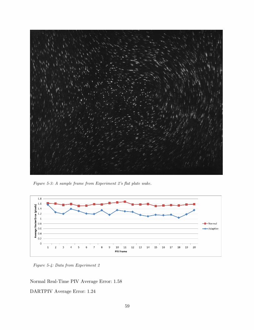
Normal Real-Time PIV Average Error: 1.58

DARTPIV Average Error: 1.24

Figure 5-4: Data from Experiment 2

Figure 5-3: A sample frame from Experiment 2’s flat plate wake.

60

However, once more, the DARTPIV approach proved more accurate. Qualitative analysis of

the vector fields showed that both approaches were able to pick up on the major flow

characteristics of the wake, however.

5.4 Experiment 3: Dual Vortices

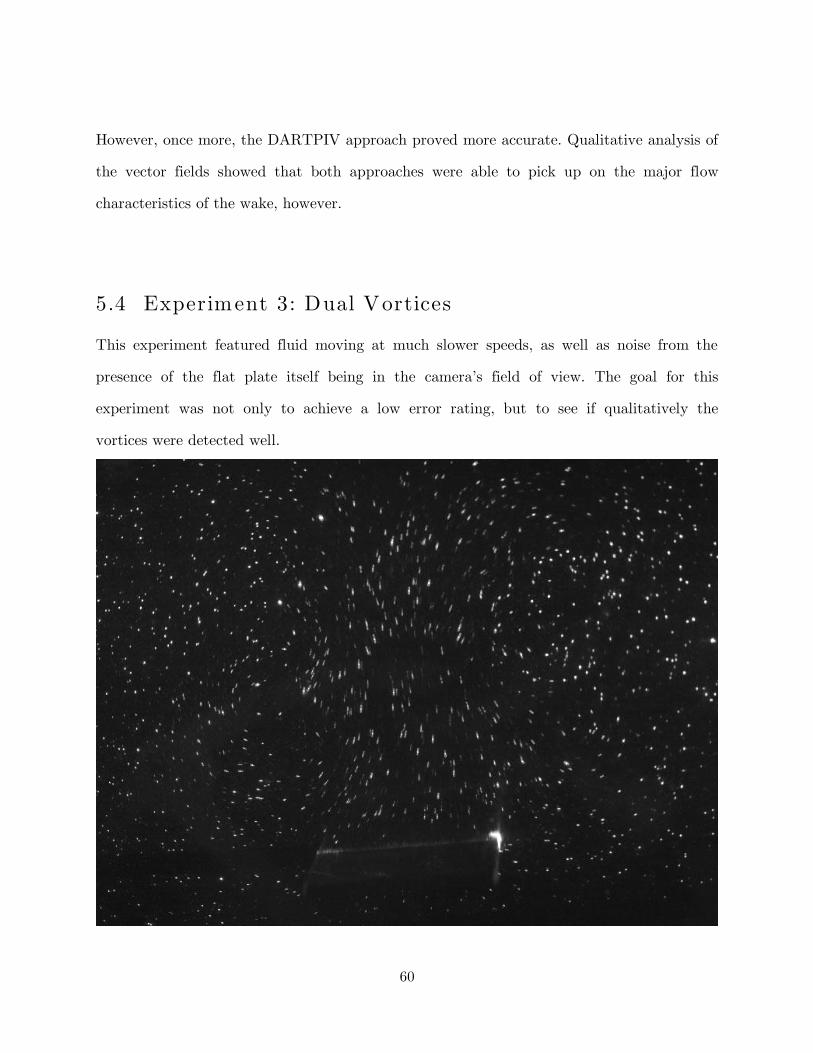
This experiment featured fluid moving at much slower speeds, as well as noise from the

presence of the flat plate itself being in the camera’s field of view. The goal for this

experiment was not only to achieve a low error rating, but to see if qualitatively the

vortices were detected well.

61

Normal Real-Time PIV Average Error: 0.91

DARTPIV Average Error: 0.80

This time around, both methods performed surprisingly well. In fact, normal real-time PIV

was almost as accurate as the DARTPIV algorithm. More importantly, however, the

vortices were picked up well in both cases, so much so that it was possible to easily visualize

them by extracting the curl of the vector field.

[figure showing curl]

5.5 Experiment 4: Free Stream Velocity

The final experiment was designed specifically to determine just how well the DARTPIV

algorithm could approximate velocities, given its ability to dynamically change interframe

time. A successful test would see it succeed in predicting the free stream velocity with high

Figure 5-6: Data from Experiment 3.

Figure 5-5: A sample frame from Experiment 3’s vortices.

62

accuracy, even at low speeds, where the normal real-time approach might simply pick up a

displacement of 0 pixels, which would not be useful.

Since DARTPIV would have to rely heavily on the dynamic interframe time in this

experiment, it would not be possible to utilize the same set of images for analysis on both

real-time PIV algorithms, as was done in the previous three experiments. This meant that

extra emphasis would have to be placed on ensuring that the data chosen to be analyzed

could be repeated reliably. To allow for an interesting yet repeatable data set, the water

tunnel pumps were first turned off and the water allowed to settle to a standstill. Then one

pump was turned on, and velocity monitored until full water circulation was achieved

(approximately 30 seconds later). The period of interest in this experiment was from the

point the pumps were turned on and fluid began to move to a few seconds after full

circulation.

This sequence was repeated thrice for each of the three PIV algorithms (DARTPIV,

normal real-time PIV, and PIVlab). PIVlab again served as the “ground truth”; due to its

high degree of accuracy and sub-pixel correlation capabilities, it was able to achieve a very

accurate representation of the displacement between frames. Once the vector field was

analyzed, the vertical components of all the vectors were averaged to determine average

fluid displacement between frames. Combining this with the known magnification factor and

interframe and exposure times, the approximate velocity could be determined at every point

over the time course of the water tunnel “ramp up”. This same approach was used to

convert the DARTPIV and normal real-time PIV results into velocity approximations over

the same “ramp up” time course.

63

The graph above details not only the repeatable nature of the experiment (notice how the

PIVlab and DARTPIV curves in particular overlap one another) but also how accurate

DARTPIV is at estimating velocities, despite having no more vector resolution than the

normal real-time PIV implementation.

5.6 Performance

Although one of the desired goals of an adaptive PIV approach is improved performance in

computation time, the implementation outlined in this paper was not able to achieve that

end. Normal real-time PIV was able to evaluate 768 vectors, each with interrogation

window sizes of 40x40 pixels over an 800x600 pixel image at a relatively spritely 14.6Hz,

leveraging the CUDA architecture to accomplish the feat.

However, the adaptive approach was only able to achieve a speed of 8.7Hz while

leveraging the CUDA architecture. Much of the time was taken up by the pre-processing

steps of determining seeding density, andbuilding and sampling from a 2-dimensional

probability distribution function. Post-processing steps such as “gridifying” the results were

also somewhat expensive, although cross-correlation remained fairly efficient.

Figure 5-7: Data from Experiment 4. [NEED TO INCLUDE DATA FROM PIVLAB]

64

Chapter 6

Conclusion and Future Work

6.1 Conclusion

In final review, we can look back at the three stated goals of adaptive real-time PIV:

improved accuracy, improved efficiency, and robustness and autonomy.

With regards to accuracy, this goal was largely achieved. Results from the first three

experiments showed that there were, on average, fewer errors from the DARTPIV approach

than that of normal real-time PIV for a variety of different flow conditions. Robustness and

autonomy were proven as well, particularly in experiment 4, which proved that the

algorithm could calculate accurate velocities for a large variety of different speeds, thanks to

the dynamic use of interframe time. Further proving that point was simply the fact that no

manual input was needed once the initial settings were in place, and the same algorithm

could adapt to a variety of different flow conditions without human intervention, which will

be a crucial aspect of real-time PIV systems moving forwards.

65

The only area in which improvement was not made was efficiency, with the frame

rate falling from 14.6Hz to 8.7Hz between normal and adaptive PIV implementations. This

was largely due to the fact that parallel processing interrogation windows means less room

for temporal improvement, even if fewer cross-correlations are needed to achieve the same

result. If an implementation that uses sequential methods is used, one would likely see a

large improvement in the efficiency of the cross-correlation step.

The results of this thesis point to one undeniable fact – that dynamic, adaptive

techniques can play a big role in improving real-time PIV. As real-time PIV improves, gains

more visibility, and becomes more widespread, researchers will continue to look for ways to

make the tool more powerful and versatile, and many of the techniques shown here may

provide the answers. The research world has only scratched the surface of what PIV can do,

but with some improvements, it can become a major agent that ushers in a new age of great

advancements in many fields, such as robot locomotion in air and underwater, smarter wind

farms, more detailed aerodynamic calculations, medical and biological applications, and

more.

6.2 Future W ork

Much of the future work related to the field of adaptive real-time PIV centers around

improving efficiency of the algorithm. Greater efficiency in pre- and post-processing steps

can dramatically improve upon the performance metrics of the technique outlined in this

paper, which would allow for more time and computing resources to be spent on ensuring

accuracy and robustness. Adding error correction steps such as outlier removal would be a

big improvement, as would interpolation to fill in the spots taken by those stray vectors. A

smoothing mask could also be used to ensure a more elegant vector field output.

Other improvements that would improve the adoption rates of this technique would

be discovering ways to implement a reliable PIV algorithm on cheaper hardware. This

would allow for the greatest future works of all – seeing how PIV techniques adapt to

66

different fields to help push research along. No other technique can illuminate the

mysterious, complex, invisible motion of fluids better than particle image velocimetry, and

developing it into a tool that can be used easily and cost effectively would be very

worthwhile.