Daron Acemoglu - Capital Deepening and Non-Balanced Economic Growth (2006)

NBER WORKING PAPER SERIES

CAPITAL DEEPENING AND NON-BALANCEDECONOMIC GROWTH

Daron AcemogluVeronica Guerrieri

Working Paper 12475http://www.nber.org/papers/w12475

NATIONAL BUREAU OF ECONOMIC RESEARCH1050 Massachusetts Avenue

Cambridge, MA 02138August 2006

We thank John Laitner, Guido Lorenzoni, Iv an Werning and seminar participants at Chicago, FederalReserve Bank of Richmond, IZA, MIT, NBER Economic Growth Group, 2005, Society of EconomicDynamics, Florence 2004 and Vancouver 2006, and Universitat of Pompeu Fabra for useful comments andAriel Burstein for help with the simulations. Acemoglu acknowledges financial support from the RussellSage Foundation and the NSF. An early version of this paper was circulated under the title “Non-BalancedEndogenous Growth”. The views expressed herein are those of the author(s) and do not necessarily reflectthe views of the National Bureau of Economic Research.

©2006 by Daron Acemoglu and Veronica Guerrieri. All rights reserved. Short sections of text, not to exceedtwo paragraphs, may be quoted without explicit permission provided that full credit, including © notice, isgiven to the source.

Capital Deepening and Non-Balanced Economic GrowthDaron Acemoglu and Veronica GuerrieriNBER Working Paper No. 12475August 2006JEL No. O30, O40, 041

ABSTRACT

This paper constructs a model of non-balanced economic growth. The main economic force is thecombination of differences in factor proportions and capital deepening. Capital deepening tends toincrease the relative output of the sector with a greater capital share, but simultaneously induces areallocation of capital and labor away from that sector. We first illustrate this force using a generaltwo-sector model. We then investigate it further using a class of models with constant elasticity ofsubstitution between two sectors and Cobb-Douglas production functions in each sector. In this classof models, non-balanced growth is shown to be consistent with an asymptotic equilibrium withconstant interest rate and capital share in national income. We also show that for realistic parametervalues, the model generates dynamics that are broadly consistent with US data. In particular, themodel generates more rapid growth of employment in less capital-intensive sectors, more rapidgrowth of real output in more capital-intensive sectors and aggregate behavior in line with the Kaldorfacts. Finally, we construct and analyze a model of “non-balanced endogenous growth,” whichextends the main results of the paper to an economy with endogenous anddirected technical change.This model shows that equilibrium will typically involve endogenous non-balanced technologicalprogress.

Daron AcemogluDepartment of EconomicsMIT, E52-380B50 Memorial DriveCambridge, MA 02142-1347and [email protected]

Veronica GuerrieriUniversity of ChicagoGraduate School of Business5807 South Woodlawn AvenueRoom 310Chicago, IL [email protected]

1 Introduction

Most models of economic growth strive to be consistent with the “Kaldor facts”, i.e., the

relative constancy of the growth rate, the capital-output ratio, the share of capital income

in GDP and the real interest rate (see Kaldor, 1963, and also Denison, 1974, Homer and

Sylla, 1991, Barro and Sala-i-Martin, 2004). Beneath this balanced picture, however, are the

patterns that Kongsamut, Rebelo and Xie (2001) refer to as the “Kuznets facts”, which concern

the systematic change in the relative importance of various sectors, in particular, agriculture,

manufacturing and services (see Kuznets, 1957, 1973, Chenery, 1960, Kongsamut, Rebelo and

Xie, 2001). While the Kaldor facts emphasize the balanced nature of economic growth, the

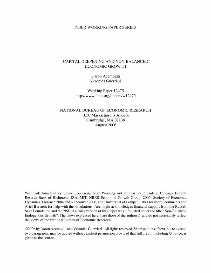
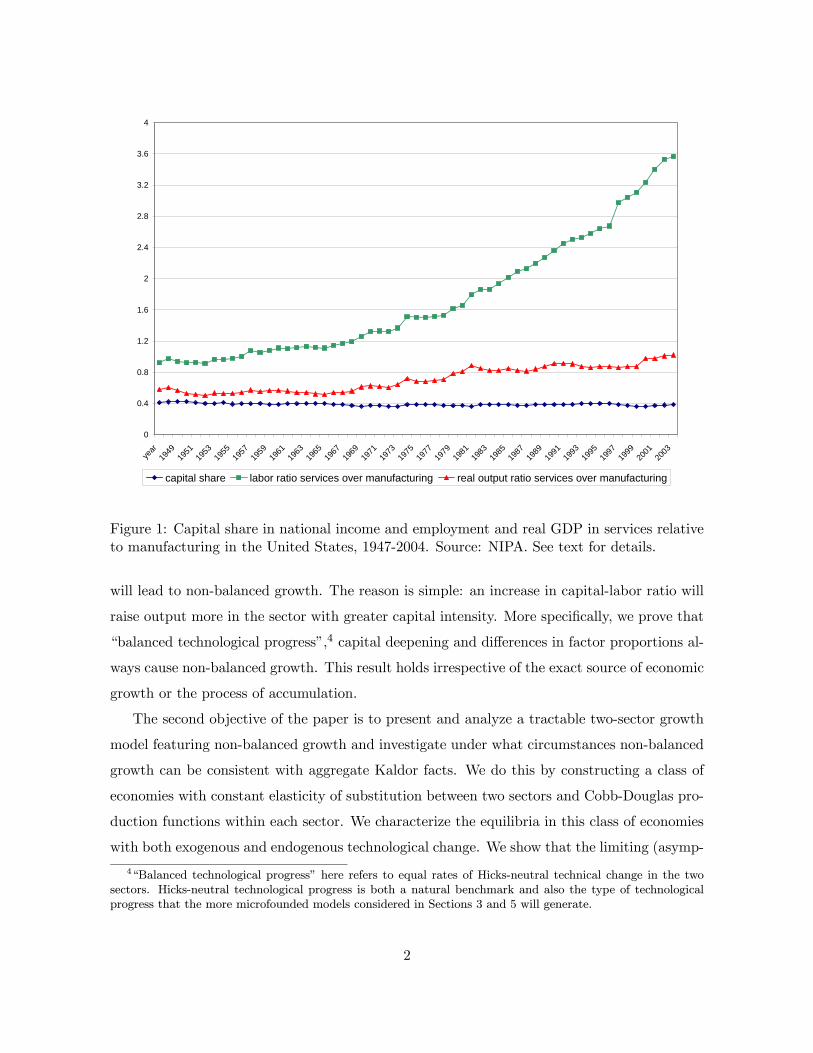
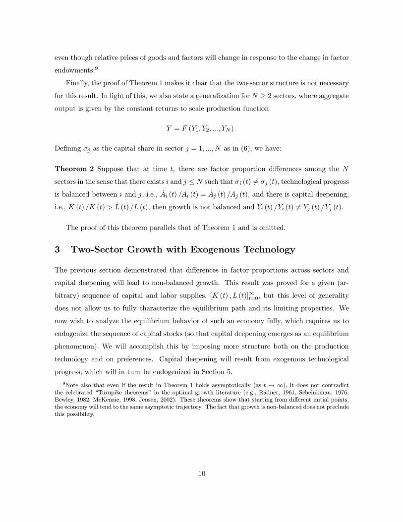
Kuznets facts highlight its non-balanced nature. Figure 1 illustrates some aspects of both the

Kaldor and Kuznets facts for postwar US; the capital share of national income is relatively

constant, whereas relative employment and output in services increase significantly.1

The Kuznets facts have motivated a small literature, which typically starts by positing

non-homothetic preferences consistent with Engel’s law.2 This literature therefore emphasizes

the demand-side reasons for non-balanced growth; the marginal rate of substitution between

different goods changes as an economy grows, directly leading to a pattern of uneven growth

between sectors. An alternative thesis, first proposed by Baumol (1967), emphasizes the po-

tential non-balanced nature of economic growth resulting from differential productivity growth

across sectors, but has received less attention in the literature.3

This paper has two aims. First, it shows that there is a natural supply-side reason, re-

lated to Baumol’s (1967) thesis, for economic growth to be non-balanced. Differences in factor

proportions across sectors (i.e., different shares of capital) combined with capital deepening

1All data are from the National Income and Product Accounts (NIPA). For details and definitions of services,manufacturing, employment, real GDP and capital share, see Appendix B.

2See, for example, Murphy, Shleifer and Vishny (1989), Matsuyama (1992), Echevarria (1997), Laitner (2000),Kongsamut, Rebelo and Xie (2001), Caselli and Coleman (2001), Gollin, Parente and Rogerson (2002). See alsothe interesting papers by Stokey (1988), Matsuyama (2002), Foellmi and Zweimuller (2002), and Buera andKaboski (2006), which derive non-homothetiticites from the presence of a “hierarchy of needs” or “hierarchyof qualities”. Finally, Hall and Jones (2006) point out that there are natural reasons for health care to bea superior good (because expected life expectancy multiplies utility) and show how this can account for theincrease in health care spending. Matsuyama (2005) presents an excellent overview of this literature.

3Two exceptions are the two recent independent papers by Ngai and Pissarides (2006) and Zuleta and Young(2006). Ngai and Pissarides (2006), for example, construct a model of multi-sector economic growth inspiredby Baumol. In Ngai and Pissarides’s model, there are exogenous Total Factor Productivity differences acrosssectors, but all sectors have identical Cobb-Douglas production functions. While both of these papers arepotentially consistent with the Kuznets and Kaldor facts, they do not contain the main contribution of ourpaper: non-balanced growth resulting from factor proportion differences and capital deepening.

1

0

0.4

0.8

1.2

1.6

2

2.4

2.8

3.2

3.6

4

year

1949

1951

1953

1955

1957

1959

1961

1963

1965

1967

1969

1971

1973

1975

1977

1979

1981

1983

1985

1987

1989

1991

1993

1995

1997

1999

2001

2003

capital share labor ratio services over manufacturing real output ratio services over manufacturing

Figure 1: Capital share in national income and employment and real GDP in services relativeto manufacturing in the United States, 1947-2004. Source: NIPA. See text for details.

will lead to non-balanced growth. The reason is simple: an increase in capital-labor ratio will

raise output more in the sector with greater capital intensity. More specifically, we prove that

“balanced technological progress”,4 capital deepening and differences in factor proportions al-

ways cause non-balanced growth. This result holds irrespective of the exact source of economic

growth or the process of accumulation.

The second objective of the paper is to present and analyze a tractable two-sector growth

model featuring non-balanced growth and investigate under what circumstances non-balanced

growth can be consistent with aggregate Kaldor facts. We do this by constructing a class of

economies with constant elasticity of substitution between two sectors and Cobb-Douglas pro-

duction functions within each sector. We characterize the equilibria in this class of economies

with both exogenous and endogenous technological change. We show that the limiting (asymp-

4“Balanced technological progress” here refers to equal rates of Hicks-neutral technical change in the twosectors. Hicks-neutral technological progress is both a natural benchmark and also the type of technologicalprogress that the more microfounded models considered in Sections 3 and 5 will generate.

2

totic) equilibrium takes a simple form and features constant but different growth rates in each

sector, constant interest rate and constant share of capital in national income.

Other properties of the limiting equilibrium of this class of economies depend on whether

the products of the two sectors are gross substitutes or complements (meaning whether the

elasticity of substitution between these products is greater than or less than one). Suppose for

this discussion that the rates of technological progress in the two sectors are similar. In this

case, when the two sectors are gross substitutes, the more capital-intensive sector dominates

the economy. The form of the equilibrium is more subtle and interesting when the elasticity of

substitution between these products is less than one; the growth rate of the economy is now

determined by the more slowly growing, less capital-intensive sector. Despite the change in

the terms of trade against the faster growing, capital-intensive sector, in equilibrium sufficient

amounts of capital and labor are deployed in this sector to ensure a faster rate of growth than

in the less capital-intensive sector.

One interesting feature is that our model economy generates non-balanced growth without

significantly deviating from the Kaldor facts. In particular, even in the limiting equilibrium

both sectors grow at positive (and unequal) rates. More importantly, when the elasticity of

substitution is less than one,5 convergence to this limiting equilibrium is typically slow and

along the transition path, growth is non-balanced, while capital share and interest rate vary

by relatively small amounts. Therefore, the equilibrium with an elasticity of substitution less

than one may be able to rationalize both non-balanced sectoral growth and the Kaldor facts.

Finally, we present and analyze a model of “non-balanced endogenous growth,” which shows

the robustness of our results to endogenous technological progress. Our analysis shows that

when sectors differ in terms of their capital intensity, equilibrium technological change will

5As we will see below, the elasticity of substitution between products will be less than one if and only if the(short-run) elasticity of substitution between labor and capital is less than one. In view of the time-series andcross-industry evidence, a short-run elasticity of substitution between labor and capital less than one appearsreasonable.For example, Hamermesh (1993), Nadiri (1970) and Nerlove (1967) survey a range of early estimates of the

elasticity of substitution, which are generally between 0.3 and 0.7. David and Van de Klundert (1965) similarlyestimate this elasticity to be in the neighborhood of 0.3. Using the translog production function, Griffin andGregory (1976) estimate elasticities of substitution for nine OECD economies between 0.06 and 0.52. Berndt(1976), on the other hand, estimates an elasticity of substitution equal to 1, but does not control for a timetrend, creating a strong bias towards 1. Using more recent data, and various different specifications, Krusell,Ohanian, Rios-Rull, and Violante (2000) and Antras (2001) also find estimates of the elasticity significantlyless than 1. Estimates implied by the response of investment to the user cost of capital also typically imply anelasticity of substitution between capital and labor significantly less than 1 (see, e.g., Chirinko, 1993, Chirinko,Fazzari and Mayer, 1999, or Mairesse, Hall and Mulkay, 1999).

3

itself be non-balanced and will not restore balanced growth between sectors. To the best of

our knowledge, despite the large literature on endogenous growth, there are no previous studies

that combine endogenous technological progress and non-balanced growth.6

A variety of evidence suggests that non-homotheticities in consumption emphasized by the

previous literature are indeed present and create a tendency towards non-balanced growth. Our

purpose in this paper is not to argue that these demand-side factors are unimportant, but to

propose and isolate an alternative supply-side force contributing to non-balanced growth and

show that it is potentially quite powerful as well. Naturally, whether or not our mechanism is

important in practice is an empirical question. In Section 4, we undertake a simple calibration

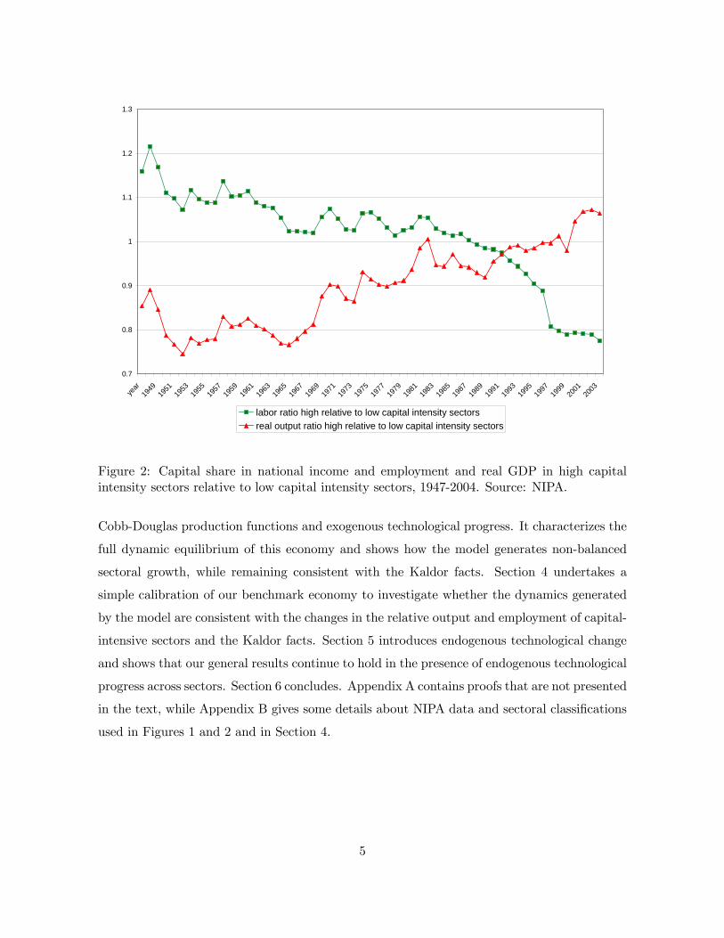
of our benchmark model to provide a preliminary investigation of this question. As a prepa-

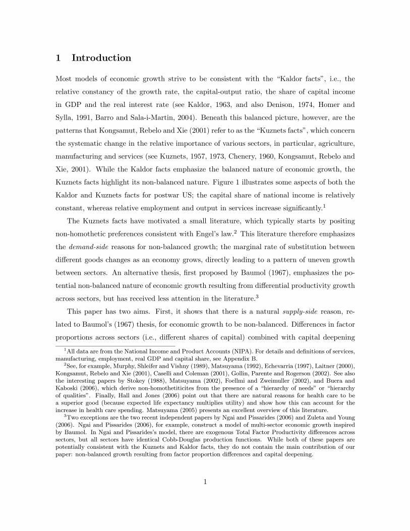
ration for this calibration, Figure 2 shows the equivalent of Figure 1, but with sectors divided

according to their capital intensity (see Appendix B for details). This figure shows a number

of important patterns: first, consistent with our qualitative predictions, there is more rapid

growth of employment in less capital-intensive sectors.7 Second, also in line with our approach,

the figure shows that the rate of growth of real GDP is faster in more capital-intensive sectors.

Notably, this contrasts with Figure 1, which showed faster growth in both employment and

real GDP for services. The opposite movements of employment and real GDP for sectors with

high and low capital intensity is a distinctive feature of our approach (for the theoretically and

empirically relevant case of the elasticity of substitution less than one). The simple calibra-

tion exercise in Section 4 also shows that our model economy generates equilibrium dynamics

consistent with both non-balanced growth at the sectoral level and the Kaldor facts at the

aggregate level. Moreover, not only the qualitative but also the quantitative implications of

our model appear to be broadly consistent with the data shown in Figure 2.

The rest of the paper is organized as follows. Section 2 shows how the combination of

factor proportions differences and capital deepening lead to non-balanced growth. Section 3

constructs a more specific model with a constant elasticity of substitution between two sectors,

6See, among others, Romer (1986, 1990), Lucas (1988), Rebelo (1991), Segerstrom, Anant and Dinopoulos(1990), Stokey (1991), Grossman and Helpman (1991a,b), Aghion and Howitt (1992), Jones (1995), Young(1993). Aghion and Howitt (1998) and Barro and Sala-i-Martin (2004) provide excellent introductions toendogenous growth theory. See also Acemoglu (2002) on models of directed technical change that featureendogenous, but balanced technological progress in different sectors. Acemoglu (2003) presents a model withnon-balanced technological progress between two sectors, but in the limiting equilibrium both sectors grow atthe same rate.

7Note also that the magnitude of changes in Figure 2 is less than those in Figure 1, which suggests thatchanges in the composition of demand between manufacturing and services are likely responsible for some ofthe changes in the sectoral composition of output experienced over the past 60 years.

4

0.7

0.8

0.9

1

1.1

1.2

1.3

year

1949

1951

1953

1955

1957

1959

1961

1963

1965

1967

1969

1971

1973

1975

1977

1979

1981

1983

1985

1987

1989

1991

1993

1995

1997

1999

2001

2003

labor ratio high relative to low capital intensity sectorsreal output ratio high relative to low capital intensity sectors

Figure 2: Capital share in national income and employment and real GDP in high capitalintensity sectors relative to low capital intensity sectors, 1947-2004. Source: NIPA.

Cobb-Douglas production functions and exogenous technological progress. It characterizes the

full dynamic equilibrium of this economy and shows how the model generates non-balanced

sectoral growth, while remaining consistent with the Kaldor facts. Section 4 undertakes a

simple calibration of our benchmark economy to investigate whether the dynamics generated

by the model are consistent with the changes in the relative output and employment of capital-

intensive sectors and the Kaldor facts. Section 5 introduces endogenous technological change

and shows that our general results continue to hold in the presence of endogenous technological

progress across sectors. Section 6 concludes. Appendix A contains proofs that are not presented

in the text, while Appendix B gives some details about NIPA data and sectoral classifications

used in Figures 1 and 2 and in Section 4.

5

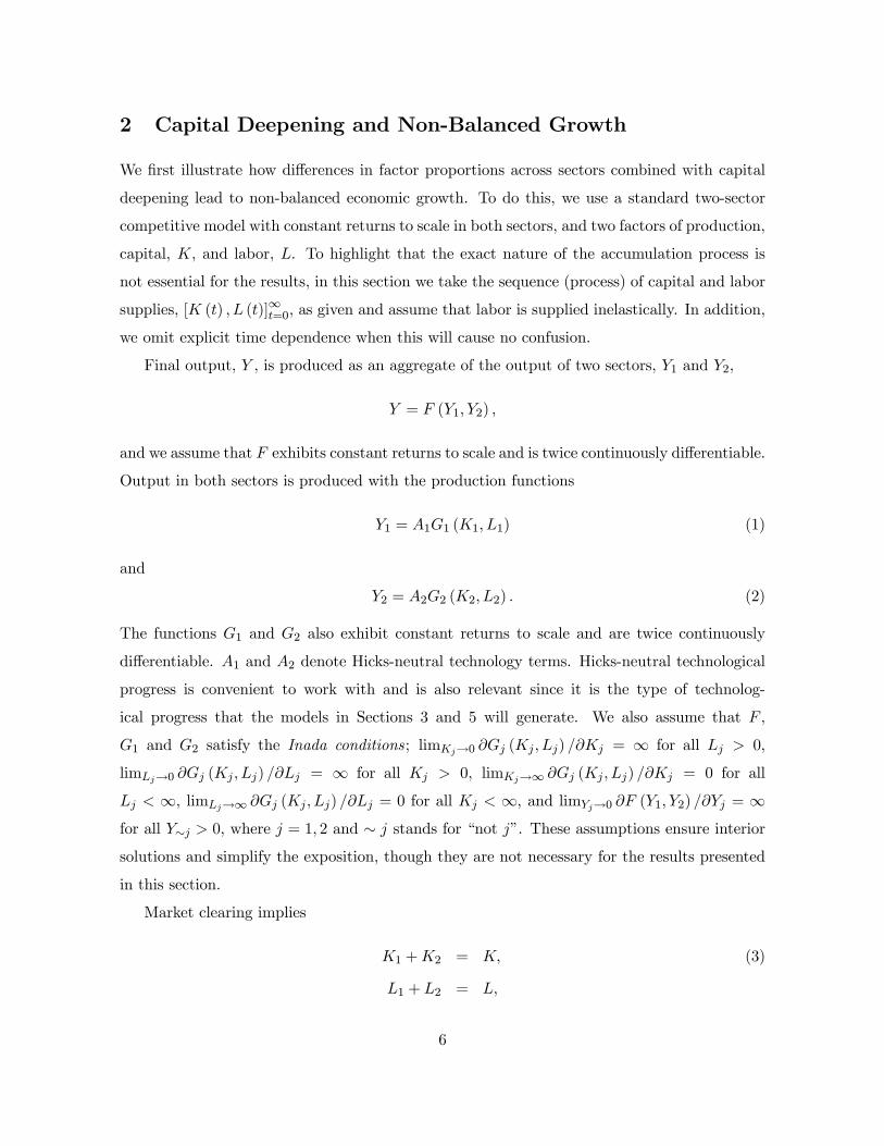
2 Capital Deepening and Non-Balanced Growth

We first illustrate how differences in factor proportions across sectors combined with capital

deepening lead to non-balanced economic growth. To do this, we use a standard two-sector

competitive model with constant returns to scale in both sectors, and two factors of production,

capital, K, and labor, L. To highlight that the exact nature of the accumulation process is

not essential for the results, in this section we take the sequence (process) of capital and labor

supplies, [K (t) , L (t)]∞t=0, as given and assume that labor is supplied inelastically. In addition,

we omit explicit time dependence when this will cause no confusion.

Final output, Y , is produced as an aggregate of the output of two sectors, Y1 and Y2,

Y = F (Y1, Y2) ,

and we assume that F exhibits constant returns to scale and is twice continuously differentiable.

Output in both sectors is produced with the production functions

Y1 = A1G1 (K1, L1) (1)

and

Y2 = A2G2 (K2, L2) . (2)

The functions G1 and G2 also exhibit constant returns to scale and are twice continuously

differentiable. A1 and A2 denote Hicks-neutral technology terms. Hicks-neutral technological

progress is convenient to work with and is also relevant since it is the type of technolog-

ical progress that the models in Sections 3 and 5 will generate. We also assume that F ,

G1 and G2 satisfy the Inada conditions; limKj→0 ∂Gj (Kj , Lj) /∂Kj = ∞ for all Lj > 0,

limLj→0 ∂Gj (Kj , Lj) /∂Lj = ∞ for all Kj > 0, limKj→∞ ∂Gj (Kj , Lj) /∂Kj = 0 for all

Lj < ∞, limLj→∞ ∂Gj (Kj , Lj) /∂Lj = 0 for all Kj < ∞, and limYj→0 ∂F (Y1, Y2) /∂Yj = ∞for all Y∼j > 0, where j = 1, 2 and ∼ j stands for “not j”. These assumptions ensure interior

solutions and simplify the exposition, though they are not necessary for the results presented

in this section.

Market clearing implies

K1 +K2 = K, (3)

L1 + L2 = L,

6

where K and L are the (potentially time-varying) supplies of capital and labor, given by the

exogenous sequences [K (t) , L (t)]∞t=0. We take these sequences to be continuosly differentiable

functions of time. Without loss of any generality, we also ignore capital depreciation.

We normalize the price of the final good to 1 in every period and denote the prices of Y1

and Y2 by p1 and p2, and wage and rental rate of capital (interest rate) by w and r. We assume

that product and factor markets are competitive, so product prices satisfy

p1p2=

∂F (Y1, Y2) /∂Y1∂F (Y1, Y2) /∂Y2

. (4)

Moreover, given the Inada conditions, the wage and the interest rate satisfy:8

w =∂A1G1 (K1, L1)

∂L1=

∂A2G2 (K2, L2)

∂L2(5)

r =∂A1G1 (K1, L1)

∂K1=

∂A2G2 (K2, L2)

∂K2.

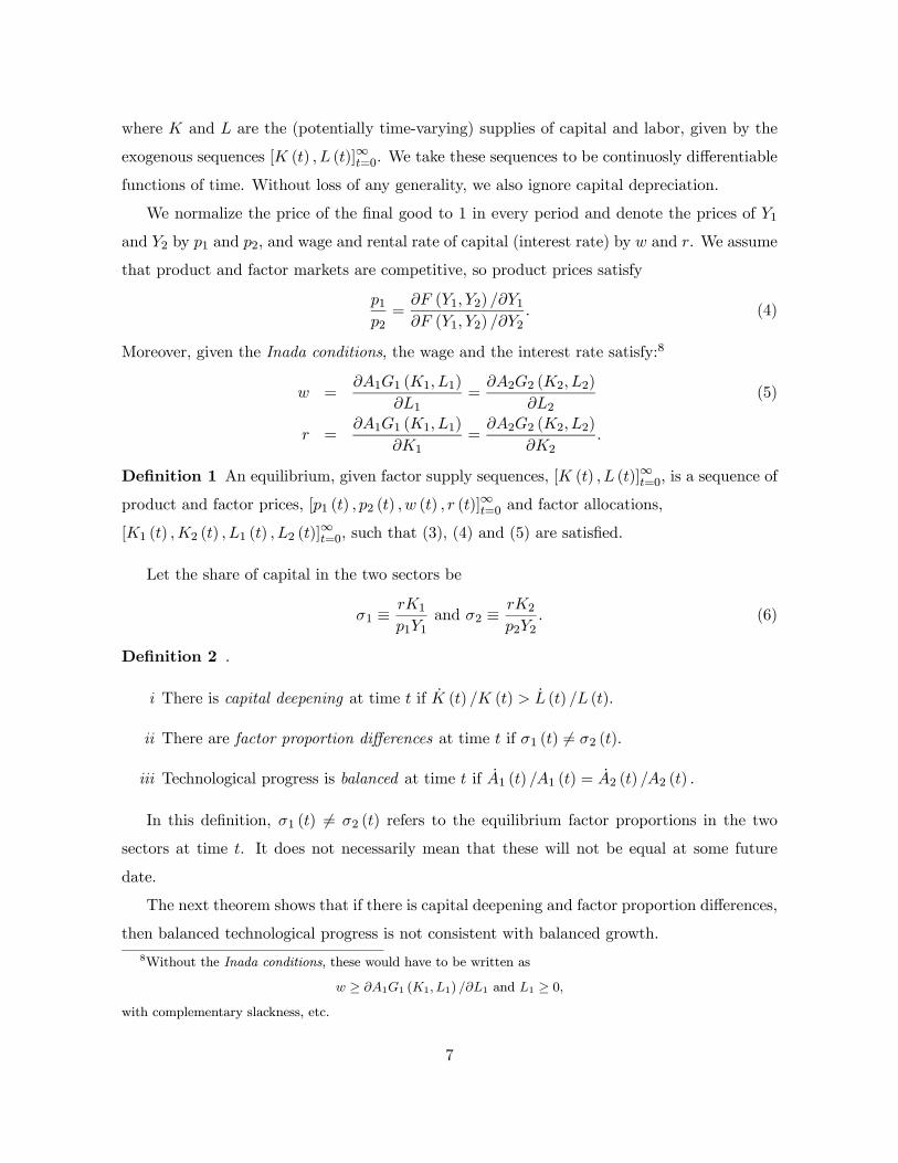
Definition 1 An equilibrium, given factor supply sequences, [K (t) , L (t)]∞t=0, is a sequence of

product and factor prices, [p1 (t) , p2 (t) , w (t) , r (t)]∞t=0 and factor allocations,

[K1 (t) ,K2 (t) , L1 (t) , L2 (t)]∞t=0, such that (3), (4) and (5) are satisfied.

Let the share of capital in the two sectors be

σ1 ≡rK1

p1Y1and σ2 ≡

rK2

p2Y2. (6)

Definition 2 .

i There is capital deepening at time t if K (t) /K (t) > L (t) /L (t).

ii There are factor proportion differences at time t if σ1 (t) 6= σ2 (t).

iii Technological progress is balanced at time t if A1 (t) /A1 (t) = A2 (t) /A2 (t) .

In this definition, σ1 (t) 6= σ2 (t) refers to the equilibrium factor proportions in the two

sectors at time t. It does not necessarily mean that these will not be equal at some future

date.

The next theorem shows that if there is capital deepening and factor proportion differences,

then balanced technological progress is not consistent with balanced growth.

8Without the Inada conditions, these would have to be written as

w ≥ ∂A1G1 (K1, L1) /∂L1 and L1 ≥ 0,

with complementary slackness, etc.

7

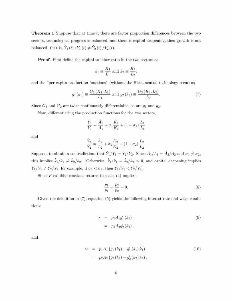
Theorem 1 Suppose that at time t, there are factor proportion differences between the two

sectors, technological progress is balanced, and there is capital deepening, then growth is not

balanced, that is, Y1 (t) /Y1 (t) 6= Y2 (t) /Y2 (t).

Proof. First define the capital to labor ratio in the two sectors as

k1 ≡K1

L1and k2 ≡

K2

L2,

and the “per capita production functions” (without the Hicks-neutral technology term) as

g1 (k1) ≡G1 (K1, L1)

L1and g2 (k2) ≡

G2 (K2, L2)

L2. (7)

Since G1 and G2 are twice continuously differentiable, so are g1 and g2.

Now, differentiating the production functions for the two sectors,

Y1Y1=

A1A1

+ σ1K1

K1+ (1− σ1)

L1L1

andY2Y2=

A2A2

+ σ2K2

K2+ (1− σ2)

L2L2

.

Suppose, to obtain a contradiction, that Y1/Y1 = Y2/Y2. Since A1/A1 = A2/A2 and σ1 6= σ2,

this implies k1/k1 6= k2/k2. [Otherwise, k1/k1 = k2/k2 > 0, and capital deepening implies

Y1/Y1 6= Y2/Y2; for example, if σ1 < σ2, then Y1/Y1 < Y2/Y2].

Since F exhibits constant returns to scale, (4) implies

p1p1=

p2p2= 0. (8)

Given the definition in (7), equation (5) yields the following interest rate and wage condi-

tions:

r = p1A1g01 (k1) (9)

= p2A2g02 (k2) ,

and

w = p1A1¡g1 (k1)− g01 (k1) k1

¢(10)

= p2A2¡g2 (k2)− g02 (k2) k2

¢.

8

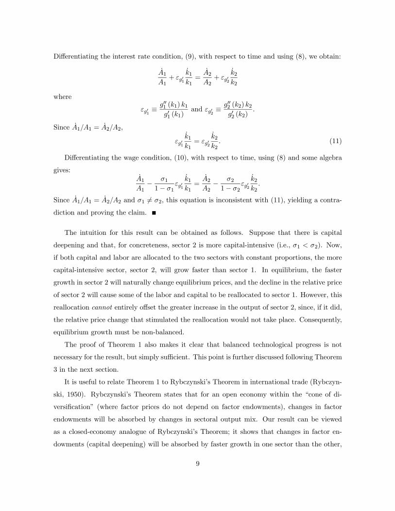
Differentiating the interest rate condition, (9), with respect to time and using (8), we obtain:

A1A1

+ εg01k1k1=

A2A2

+ εg02k2k2

where

εg01 ≡g001 (k1) k1g01 (k1)

and εg02 ≡g002 (k2) k2g02 (k2)

.

Since A1/A1 = A2/A2,

εg01k1k1= εg02

k2k2. (11)

Differentiating the wage condition, (10), with respect to time, using (8) and some algebra

gives:A1A1− σ11− σ1

εg01k1k1=

A2A2− σ21− σ2

εg02k2k2.

Since A1/A1 = A2/A2 and σ1 6= σ2, this equation is inconsistent with (11), yielding a contra-

diction and proving the claim.

The intuition for this result can be obtained as follows. Suppose that there is capital

deepening and that, for concreteness, sector 2 is more capital-intensive (i.e., σ1 < σ2). Now,

if both capital and labor are allocated to the two sectors with constant proportions, the more

capital-intensive sector, sector 2, will grow faster than sector 1. In equilibrium, the faster

growth in sector 2 will naturally change equilibrium prices, and the decline in the relative price

of sector 2 will cause some of the labor and capital to be reallocated to sector 1. However, this

reallocation cannot entirely offset the greater increase in the output of sector 2, since, if it did,

the relative price change that stimulated the reallocation would not take place. Consequently,

equilibrium growth must be non-balanced.

The proof of Theorem 1 also makes it clear that balanced technological progress is not

necessary for the result, but simply sufficient. This point is further discussed following Theorem

3 in the next section.

It is useful to relate Theorem 1 to Rybczynski’s Theorem in international trade (Rybczyn-

ski, 1950). Rybczynski’s Theorem states that for an open economy within the “cone of di-

versification” (where factor prices do not depend on factor endowments), changes in factor

endowments will be absorbed by changes in sectoral output mix. Our result can be viewed

as a closed-economy analogue of Rybczynski’s Theorem; it shows that changes in factor en-

dowments (capital deepening) will be absorbed by faster growth in one sector than the other,

9

even though relative prices of goods and factors will change in response to the change in factor

endowments.9

Finally, the proof of Theorem 1 makes it clear that the two-sector structure is not necessary

for this result. In light of this, we also state a generalization for N ≥ 2 sectors, where aggregateoutput is given by the constant returns to scale production function

Y = F (Y1, Y2, ..., YN) .

Defining σj as the capital share in sector j = 1, ..., N as in (6), we have:

Theorem 2 Suppose that at time t, there are factor proportion differences among the N

sectors in the sense that there exists i and j ≤ N such that σi (t) 6= σj (t), technological progress

is balanced between i and j, i.e., Ai (t) /Ai (t) = Aj (t) /Aj (t), and there is capital deepening,

i.e., K (t) /K (t) > L (t) /L (t), then growth is not balanced and Yi (t) /Yi (t) 6= Yj (t) /Yj (t).

The proof of this theorem parallels that of Theorem 1 and is omitted.

3 Two-Sector Growth with Exogenous Technology

The previous section demonstrated that differences in factor proportions across sectors and

capital deepening will lead to non-balanced growth. This result was proved for a given (ar-

bitrary) sequence of capital and labor supplies, [K (t) , L (t)]∞t=0, but this level of generality

does not allow us to fully characterize the equilibrium path and its limiting properties. We

now wish to analyze the equilibrium behavior of such an economy fully, which requires us to

endogenize the sequence of capital stocks (so that capital deepening emerges as an equilibrium

phenomenon). We will accomplish this by imposing more structure both on the production

technology and on preferences. Capital deepening will result from exogenous technological

progress, which will in turn be endogenized in Section 5.

9Note also that even if the result in Theorem 1 holds asymptotically (as t → ∞), it does not contradictthe celebrated “Turnpike theorems” in the optimal growth literature (e.g., Radner, 1961, Scheinkman, 1976,Bewley, 1982, McKenzie, 1998, Jensen, 2002). These theorems show that starting from different initial points,the economy will tend to the same asymptotic trajectory. The fact that growth is non-balanced does not precludethis possibility.

10

3.1 Demographics, Preferences and Technology

The economy consists of L (t) workers at time t, supplying their labor inelastically. There is

exponential population growth,

L (t) = exp (nt)L (0) . (12)

We assume that all households have constant relative risk aversion (CRRA) preferences over

total household consumption (rather than per capita consumption), and all population growth

takes place within existing households (thus there is no growth in the number of households).10

This implies that the economy admits a representative agent with CRRA preferences:Z ∞

0

C(t)1−θ − 11− θ

e−ρtdt, (13)

where C (t) is aggregate consumption at time t, ρ is the rate of time preferences and θ ≥ 0is the inverse of the intertemporal elasticity of substitution (or the coefficient of relative risk

aversion). We again drop time arguments to simplify the notation whenever this causes no

confusion. We also continue to assume that there is no depreciation of capital.

The flow budget constraint for the representative consumer is:

K = rK + wL+Π−C. (14)

Here w is the equilibrium wage rate and r is the equilibrium interest rate, K and L denote

the total capital stock and the total labor force in the economy, and Π is total net corporate

profits received by the consumers (which will be equal to zero in this section).

The unique final good is produced by combining the output of two sectors with an elasticity

of substitution ε ∈ [0,∞):

Y =

∙γY

ε−1ε

1 + (1− γ)Yε−1ε

2

¸ εε−1

, (15)

where γ is a distribution parameter which determines the relative importance of the two goods

in the aggregate production.

The resource constraint of the economy, in turn, requires consumption and investment to

be less than total output, Y = rK + wL+Π, thus

K + C ≤ Y. (16)

10The alternative would be to specify population growth taking place at the extensive margin, in which casethe discount rate of the representative agent would be ρ − n rather than ρ, without any important changes inthe analysis.

11

The two goods Y1 and Y2 are produced competitively using constant elasticity of substitu-

tion (CES) production functions with elasticity of substitution between intermediates equal to

ν > 1:

Y1 =

µZ M1

0y1(i)

ν−1ν di

¶ νν−1

and Y2 =

µZ M2

0y2(i)

ν−1ν di

¶ νν−1

, (17)

where y1(i)’s and y2(i)’s denote the intermediates in the sectors that have different capi-

tal/labor ratios, and M1 and M2 represent the technology terms. In particular M1 denotes

the number of intermediates in sector 1 and M2 the number of intermediate goods in sector

2. This structure is particularly useful since it can also be used for the analysis of endogenous

growth in Section 5.

Intermediate goods are produced with the following Cobb-Douglas technologies

y1(i) = l1(i)α1k1(i)

1−α1 and y2 (i) = l2 (i)α2 k2 (i)

1−α2 , (18)

where l1(i) and k1(i) are labor and capital used in the production of good i of sector 1 and

l2 (i) and k2 (i) are labor and capital used in the production of good i of sector 2.11

The parameters α1 and α2 determine which sector is more “capital intensive”.12 When

α1 > α2, sector 1 is less capital intensive, while the converse applies when α1 < α2. In the rest

of the analysis, we assume that

α1 > α2, (A1)

which only rules out the case where α1 = α2, since the two sectors are otherwise identical

and the labeling of the sector with the lower capital share as sector 1 is without loss of any

generality.

All factor markets are competitive, and market clearing for the two factors implyZ M1

0l1(i)di+

Z M2

0l2 (i) di ≡ L1 + L2 = L, (19)

and Z M1

0k1(i)di+

Z M2

0k2 (i) di ≡ K1 +K2 = K, (20)

11Strictly speaking, we should have two indices, i1 ∈M1 and i2 ∈M2, whereMj is the set of intermediatesof type j, and Mj is the measure of the setMj . We simplify the notation by using a generic i to denote bothindices, and let the context determine which index is being referred to.12We use the term “capital intensive” as corresponding to a greater share of capital in value added, i.e.,

σ2 > σ1 in terms of the notation of the previous section. While this share is constant because of the Cobb-Douglas technologies, the equilibrium ratios of capital to labor in the two sectors depend on prices.

12

where the first set of equalities in these equations define K1, L1,K2 and L2 as the levels of

capital and labor used in the two sectors, and the second set of equalities impose market

clearing.

The number of intermediate goods in the two sectors evolve at the exogenous rates

M1

M1= m1 and

M2

M2= m2. (21)

Since M1 and M2 determine productivity in their respective sectors, we will refer to them as

“technology”. In this section, we assume that all intermediates are also produced competitively

(i.e., any firm can produce any of the existing intermediates). In Section 5, we will modify

this assumption and assume that new intermediates are invented by R&D and the firm that

invents a new intermediate has a fully-enforced perpetual patent for its production.

3.2 Equilibrium

Recall that w and r denote the wage and the capital rental rate, and p1 and p2 denote the

prices of the Y1 and Y2 goods, with the price of the final good normalized to one. Let [q1(i)]M1i=1

and [q2(i)]M2i=1 be the prices for labor-intensive and capital-intensive intermediates.

Definition 3 An equilibrium is given by paths for factor, intermediate and final goods prices

r, w, [q1(i)]M1i=1 , [q2(i)]

M2i=1 , p1 and p2, employment and capital allocation [l1(i)]

M1i=1 , [l2(i)]

M2i=1 ,

[k1(i)]M1i=1 , [k2(i)]

M2i=1 such that firms maximize profits and markets clear, and consumption and

savings decisions, C and K, maximize consumer utility.

It is useful to break the characterization of equilibrium into two pieces: static and dynamic.

The static part takes the state variables of the economy, which are the capital stock, the labor

supply and the technology, K, L,M1 andM2, as given and determines the allocation of capital

and labor across sectors and factor and good prices. The dynamic part of the equilibrium

determines the evolution of the endogenous state variable, K (the dynamic behavior of L is

given by (12) and those of M1 and M2 by (21)).

Our choice of numeraire implies that the price of the final good, P , satisfies:

1 ≡ P =£γεp1−ε1 + (1− γ)ε p1−ε2

¤ 11−ε .

13

Next, since Y1 and Y2 are supplied competitively, their prices are equal to the value of their

marginal product, thus

p1 = γ

µY1Y

¶− 1ε

and p2 = (1− γ)

µY2Y

¶− 1ε

, (22)

and the demands for intermediates, y1(i) and y2(i), are given by the familiar isoelastic demand

curves:q1(i)

p1=

µy1(i)

Y1

¶− 1ν

andq2(i)

p2=

µy2(i)

Y2

¶− 1ν

. (23)

Since all intermediates are produced competitively, prices must equal marginal cost. More-

over, given the production functions in (18), the marginal costs of producing intermediates

take the familiar Cobb-Douglas form,

mc1 (i) = α−α11 (1− α1)α1−1 r1−α1wα1 and mc2 (i) = α−α22 (1− α2)

α2−1 r1−α2wα2 .

Therefore, at all points in time, intermediate prices satisfy

q1(i) = α1 (1− α1)α1−1 r1−α1wα1 , (24)

and

q2(i) = α2 (1− α2)α2−1 r1−α2wα2 , (25)

for all i.

Equations (24) and (25) imply that all intermediates in each sector sell at the same price

q1 = q1(i) for all i ≤ M1 and q2 = q2(i) for all i ≤ M2. This combined with (23) implies that

the demand for, and the production of, the same type of intermediate will be the same. Thus:

y1(i) = l1 (i)α1 k1 (i)

1−α1

= lα11 k1−α11 = y1 ∀i ≤M1

y2(i) = l2 (i)α2 k2 (i)

1−α2

= lα22 k1−α22 = y2 ∀i ≤M2,

where l1 and k1 are the levels of employment and capital used in each intermediate of sector

1, and l2 and k2 are the levels of employment and capital used for intermediates in sector 2.

Market clearing conditions, (19) and (20), then imply that l1 = L1/M1, k1 = K1/M1,

l2 = L2/M2 and k2 = K2/M2, so we have the output of each intermediate in the two sectors as

y1 =Lα11 K1−α1

1

M1and y2 =

Lα22 K1−α2

2

M2. (26)

14

Substituting (26) into (17), we obtain the total supply of labor- and capital-intensive goods

as

Y1 =M1

ν−11 Lα1

1 K1−α11 and Y2 =M

1ν−12 Lα2

2 K1−α22 . (27)

Comparing these (derived) production functions to (1) and (2) highlights that in this economy,

the production functions G1 and G2 from the previous section take Cobb-Douglas forms,

with one sector always having a higher share of capital than the other sector, and also that

A1 ≡M1

ν−11 and A2 ≡M

1ν−12 .

In addition, combining (27) with (15) implies that the aggregate output of the economy is:

Y =

"γ

µM

1ν−11 Lα1

1 K1−α11

¶ ε−1ε

+ (1− γ)

µM

1ν−12 Lα2

2 K1−α22

¶ ε−1ε

# εε−1

. (28)

Finally, factor prices and the allocation of labor and capital between the two sectors are

determined by:13

w = γα1

µY

Y1

¶ 1ε Y1L1

(29)

w = (1− γ)α2

µY

Y2

¶1ε Y2L2

(30)

r = γ (1− α1)

µY

Y1

¶ 1ε Y1K1

(31)

r = (1− γ) (1− α2)

µY

Y2

¶ 1ε Y2K2

. (32)

These factor prices take the familiar form, equal to the marginal product of a factor from (28).

3.3 Static Equilibrium: Comparative Statics

Let us now analyze how changes in the state variables, L,K,M1 andM2, impact on equilibrium

factor prices and factor shares. As noted in the Introduction, the case with ε < 1 is of greater

interest (and empirically more relevant as pointed out in footnote 5), so, throughout, we focus

on this case (though we give the result for the case in which ε > 1, and we only omit the

standard case with ε = 1 to avoid repetition).

13To obtain these equations, start with the cost functions above, and derive the demand for factors by using

Shepherd’s Lemma. For example, for the sector 1, these are l1 =³

α11−α1

rw

´1−α1y1 and k1 =

³α1

1−α1rw

´−α1y1.

Combine these two equations to derive the equilibrium relationship between r and w. Then using equation (24),eliminate r to obtain a relationship between w and q1. Finally, combining this relationship with the demandcurve in (23), the market clearing conditions, (19) and (20), and using (27) yields (29). The other equations areobtained similarly.

15

Let us denote the fraction of capital and labor employed in the labor-intensive sector by

κ ≡ K1/K and λ ≡ L1/L (clearly 1 − κ ≡ K2/K and 1 − λ ≡ L2/L). Combining equations

(29), (30), (31) and (32), we obtain:

κ =

"1 +

µ1− α21− α1

¶µ1− γ

γ

¶µY1Y2

¶ 1−εε

#−1(33)

and

λ =

∙µ1− α11− α2

¶µα2α1

¶µ1− κ

κ

¶+ 1

¸−1. (34)

Equation (34) makes it clear that the share of labor in sector 1, λ, is monotonically increasing

in the share of capital in sector 1, κ. We next determine how these two shares change with

capital accumulation and technological change.

Proposition 1 In equilibrium,

1.

d lnκ

d lnK= − d lnκ

d lnL=

(1− ε) (α1 − α2) (1− κ)

1 + (1− ε) (α1 − α2) (κ− λ)> 0⇔ (α1 − α2) (1− ε) > 0. (35)

2.d lnκ

d lnM2= − d lnκ

d lnM1=

(1− ε) (1− κ) /(ν − 1)1 + (1− ε) (α1 − α2) (κ− λ)

> 0⇔ ε < 1. (36)

The proof of this proposition is straightforward and is omitted.

Equation (35), part 1 of the proposition, states that when the elasticity of substitution be-

tween sectors, ε, is less than 1, the fraction of capital allocated to the capital-intensive sector

declines in the stock of capital (and conversely, when ε > 1, this fraction is increasing in the

stock of capital). To obtain the intuition for this comparative static, which is useful for under-

standing many of the results that will follow, note that if K increases and κ remains constant,

then the capital-intensive sector, sector 2, will grow by more than sector 1. Equilibrium prices

given in (22) then imply that when ε < 1 the relative price of the capital-intensive sector will

fall more than proportionately, inducing a greater fraction of capital to be allocated to the less

capital-intensive sector 1. The intuition for the converse result when ε > 1 is straightforward.

Moreover, equation (36) implies that when the elasticity of substitution, ε, is less than one,

an improvement in the technology of a sector causes the share of capital going to that sector

to fall. The intuition is again the same: when ε < 1, increased production in a sector causes

16

a more than proportional decline in its relative price, inducing a reallocation of capital away

from it towards the other sector (again the converse results and intuition apply when ε > 1).

Proposition 1 gives only the comparative statics for κ. Equation (34) immediately implies

that the same comparative statics apply to λ and thus yields the following corollary:

Corollary 1 In equilibrium,

1.d lnλ

d lnK= −d lnλ

d lnL> 0⇔ (α1 − α2) (1− ε) > 0.

2.d lnλ

d lnM2= − d lnλ

d lnM1> 0⇔ ε < 1.

Next, combining (29) and (31), we also obtain relative factor prices as

w

r=

α11− α1

µκK

λL

¶, (37)

and the capital share in the economy as:14

σK ≡rK

Y= 1− γα1

µY1Y

¶ ε−1ε

λ−1. (38)

Proposition 2 In equilibrium,

1.d ln (w/r)

d lnK= −d ln (w/r)

d lnL=

1

1 + (1− ε) (α1 − α2) (κ− λ)> 0.

2.

d ln (w/r)

d lnM2= −d ln (w/r)

d lnM1= − (1− ε) (κ− λ) /(ν − 1)

1 + (1− ε) (α1 − α2) (κ− λ)< 0⇔ (α1 − α2) (1− ε) > 0.

3.d lnσKd lnK

< 0⇔ ε < 1. (39)

4.d lnσKd lnM2

= −d lnσKd lnM1

< 0⇔ (α1 − α2) (1− ε) > 0. (40)

14Note that σK refers to the share of capital in national income, and is thus different from the capital sharesin the previous section, which were sector specific. Sector-specific capital shares are constant here because ofthe Cobb-Douglas production functions (in particular, σ1 = α1 and σ2 = α2).

17

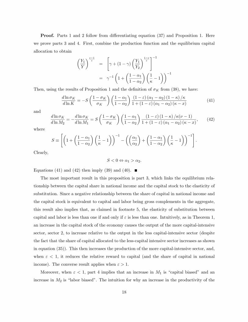
Proof. Parts 1 and 2 follow from differentiating equation (37) and Proposition 1. Here

we prove parts 3 and 4. First, combine the production function and the equilibrium capital

allocation to obtain µY1Y

¶ ε−1ε

=

"γ + (1− γ)

µY1Y2

¶1−εε

#−1

= γ−1µ1 +

µ1− α11− α2

¶µ1

κ− 1¶¶−1

Then, using the results of Proposition 1 and the definition of σK from (38), we have:

d lnσKd lnK

= −Sµ1− σKσK

¶µ1− α11− α2

¶(1− ε) (α1 − α2) (1− κ) /κ

1 + (1− ε) (α1 − α2) (κ− x)(41)

andd lnσKd lnM2

= −d lnσKd lnM1

= S

µ1− σKσK

¶µ1− α11− α2

¶(1− ε) (1− κ) /κ(ν − 1)

1 + (1− ε) (α1 − α2) (κ− x), (42)

where

S ≡"µ1 +

µ1− α11− α2

¶µ1

κ− 1¶¶−1

−µµ

α1α2

¶+

µ1− α11− α2

¶µ1

κ− 1¶¶−1#

.

Clearly,

S < 0⇔ α1 > α2.

Equations (41) and (42) then imply (39) and (40).

The most important result in this proposition is part 3, which links the equilibrium rela-

tionship between the capital share in national income and the capital stock to the elasticity of

substitution. Since a negative relationship between the share of capital in national income and

the capital stock is equivalent to capital and labor being gross complements in the aggregate,

this result also implies that, as claimed in footnote 5, the elasticity of substitution between

capital and labor is less than one if and only if ε is less than one. Intuitively, as in Theorem 1,

an increase in the capital stock of the economy causes the output of the more capital-intensive

sector, sector 2, to increase relative to the output in the less capital-intensive sector (despite

the fact that the share of capital allocated to the less-capital intensive sector increases as shown

in equation (35)). This then increases the production of the more capital-intensive sector, and,

when ε < 1, it reduces the relative reward to capital (and the share of capital in national

income). The converse result applies when ε > 1.

Moreover, when ε < 1, part 4 implies that an increase in M1 is “capital biased” and an

increase in M2 is “labor biased”. The intuition for why an increase in the productivity of the

18

sector that is intensive in capital is biased toward labor (and vice versa) is once again similar:

when the elasticity of substitution between the two sectors, ε, is less than one, an increase in

the output of a sector (this time driven by a change in technology) decreases its price more than

proportionately, thus reducing the relative compensation of the factor used more intensively in

that sector (see Acemoglu, 2002). When ε > 1, we have the converse pattern, and an increase

in M2 is “capital biased,” while an increase in M1 is “labor biased”

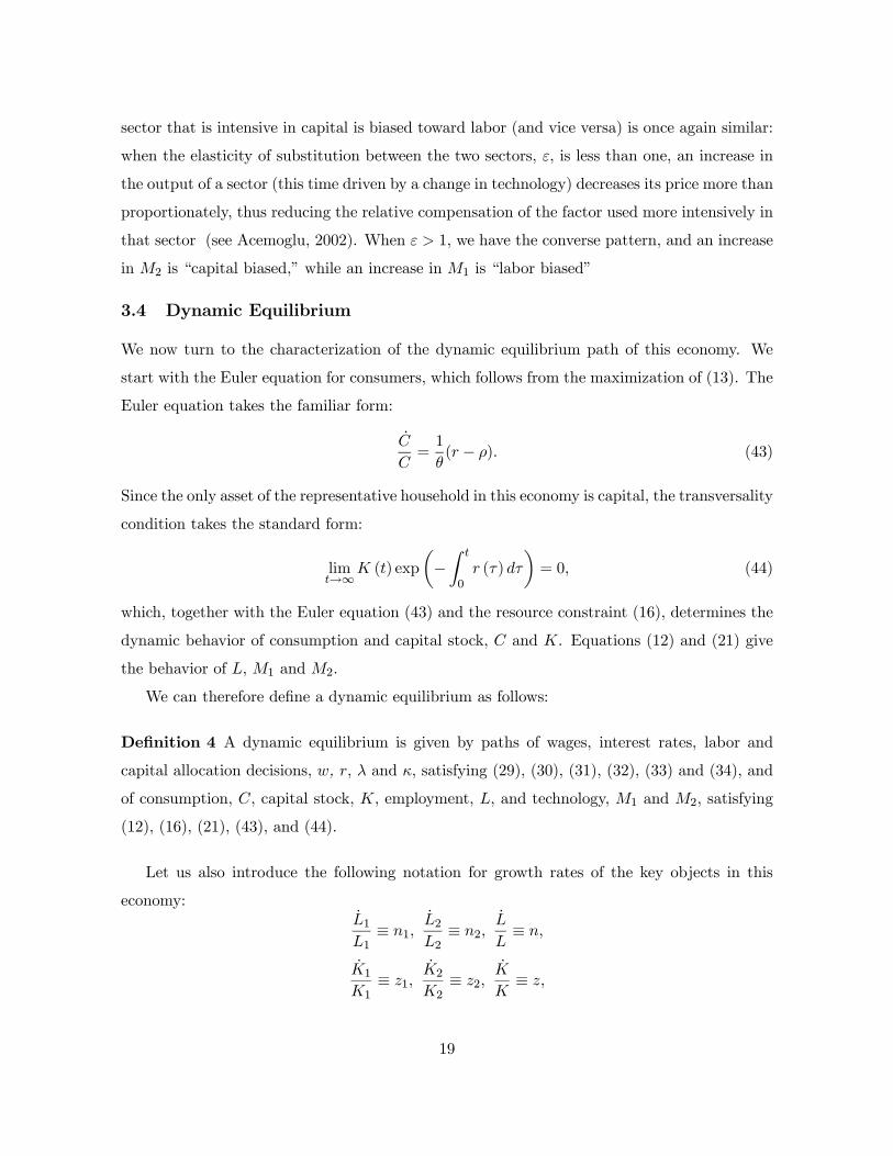
3.4 Dynamic Equilibrium

We now turn to the characterization of the dynamic equilibrium path of this economy. We

start with the Euler equation for consumers, which follows from the maximization of (13). The

Euler equation takes the familiar form:

C

C=1

θ(r − ρ). (43)

Since the only asset of the representative household in this economy is capital, the transversality

condition takes the standard form:

limt→∞

K (t) exp

µ−Z t

0r (τ) dτ

¶= 0, (44)

which, together with the Euler equation (43) and the resource constraint (16), determines the

dynamic behavior of consumption and capital stock, C and K. Equations (12) and (21) give

the behavior of L, M1 and M2.

We can therefore define a dynamic equilibrium as follows:

Definition 4 A dynamic equilibrium is given by paths of wages, interest rates, labor and

capital allocation decisions, w, r, λ and κ, satisfying (29), (30), (31), (32), (33) and (34), and

of consumption, C, capital stock, K, employment, L, and technology, M1 and M2, satisfying

(12), (16), (21), (43), and (44).

Let us also introduce the following notation for growth rates of the key objects in this

economy:L1L1≡ n1,

L2L2≡ n2,

L

L≡ n,

K1

K1≡ z1,

K2

K2≡ z2,

K

K≡ z,

19

Y1Y1≡ g1,

Y2Y2≡ g2,

Y

Y≡ g,

so that ns and zs denote the growth rate of labor and capital stock, ms denotes the growth

rate of technology, and gs denotes the growth rate of output in sector s. Moreover, whenever

they exist, we denote the corresponding asymptotic growth rates by asterisks, i.e.,

n∗s = limt→∞

ns , z∗s = lim

t→∞zs and g∗s = lim

t→∞gs.

Similarly denote the asymptotic capital and labor allocation decisions by asterisks

κ∗ = limt→∞

κ and λ∗ = limt→∞

λ.

We now state and prove two lemmas that will be useful both in this section and again in

Section 5.

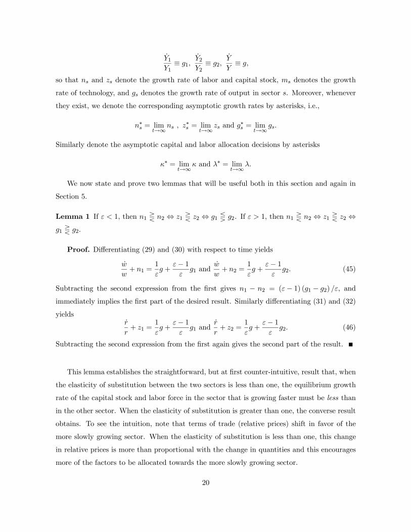
Lemma 1 If ε < 1, then n1 R n2 ⇔ z1 R z2 ⇔ g1 Q g2. If ε > 1, then n1 R n2 ⇔ z1 R z2 ⇔g1 R g2.

Proof. Differentiating (29) and (30) with respect to time yields

w

w+ n1 =

1

εg +

ε− 1ε

g1 andw

w+ n2 =

1

εg +

ε− 1ε

g2. (45)

Subtracting the second expression from the first gives n1 − n2 = (ε− 1) (g1 − g2) /ε, and

immediately implies the first part of the desired result. Similarly differentiating (31) and (32)

yieldsr

r+ z1 =

1

εg +

ε− 1ε

g1 andr

r+ z2 =

1

εg +

ε− 1ε

g2. (46)

Subtracting the second expression from the first again gives the second part of the result.

This lemma establishes the straightforward, but at first counter-intuitive, result that, when

the elasticity of substitution between the two sectors is less than one, the equilibrium growth

rate of the capital stock and labor force in the sector that is growing faster must be less than

in the other sector. When the elasticity of substitution is greater than one, the converse result

obtains. To see the intuition, note that terms of trade (relative prices) shift in favor of the

more slowly growing sector. When the elasticity of substitution is less than one, this change

in relative prices is more than proportional with the change in quantities and this encourages

more of the factors to be allocated towards the more slowly growing sector.

20

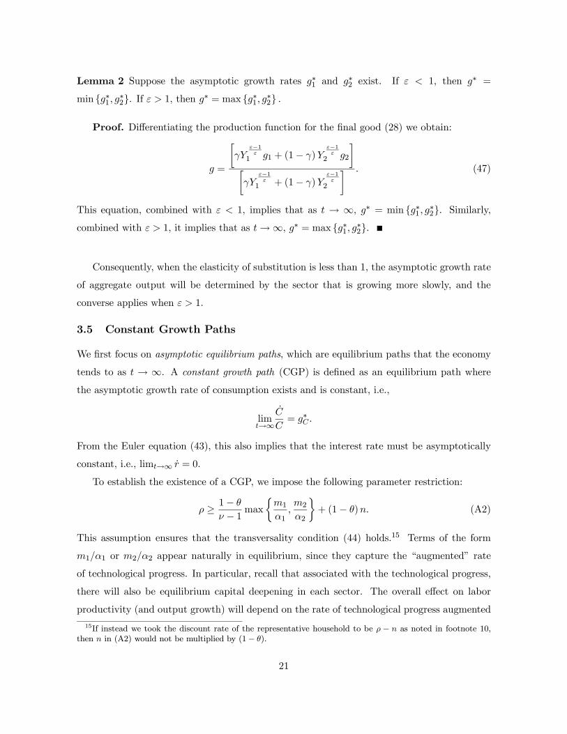
Lemma 2 Suppose the asymptotic growth rates g∗1 and g∗2 exist. If ε < 1, then g∗ =

min {g∗1, g∗2}. If ε > 1, then g∗ = max {g∗1, g∗2} .

Proof. Differentiating the production function for the final good (28) we obtain:

g =

∙γY

ε−1ε

1 g1 + (1− γ)Yε−1ε

2 g2

¸∙γY

ε−1ε

1 + (1− γ)Yε−1ε

2

¸ . (47)

This equation, combined with ε < 1, implies that as t → ∞, g∗ = min {g∗1, g∗2}. Similarly,combined with ε > 1, it implies that as t→∞, g∗ = max {g∗1, g∗2}.

Consequently, when the elasticity of substitution is less than 1, the asymptotic growth rate

of aggregate output will be determined by the sector that is growing more slowly, and the

converse applies when ε > 1.

3.5 Constant Growth Paths

We first focus on asymptotic equilibrium paths, which are equilibrium paths that the economy

tends to as t → ∞. A constant growth path (CGP) is defined as an equilibrium path where

the asymptotic growth rate of consumption exists and is constant, i.e.,

limt→∞

C

C= g∗C .

From the Euler equation (43), this also implies that the interest rate must be asymptotically

constant, i.e., limt→∞ r = 0.

To establish the existence of a CGP, we impose the following parameter restriction:

ρ ≥ 1− θ

ν − 1 max½m1

α1,m2

α2

¾+ (1− θ)n. (A2)

This assumption ensures that the transversality condition (44) holds.15 Terms of the form

m1/α1 or m2/α2 appear naturally in equilibrium, since they capture the “augmented” rate

of technological progress. In particular, recall that associated with the technological progress,

there will also be equilibrium capital deepening in each sector. The overall effect on labor

productivity (and output growth) will depend on the rate of technological progress augmented

15If instead we took the discount rate of the representative household to be ρ − n as noted in footnote 10,then n in (A2) would not be multiplied by (1− θ).

21

with the rate of capital deepening. The terms m1/α1 or m2/α2 capture this, since a lower α1

or α2 corresponds to a greater share of capital in the relevant sector, and thus a higher rate of

augmented technological progress for a given rate of Hicks-neutral technological change. In this

light, Assumption A2 can be understood as implying that the augmented rate of technological

progress should be low enough to satisfy the transversality condition (44).

The next theorem is the main result of this part of the paper and characterizes the relatively

simple form of the CGP in the presence of non-balanced growth. Although we characterize a

CGP, in the sense that aggregate output grows at a constant rate, it is noteworthy that growth

is non-balanced since output, capital and employment in the two sectors grow at different rates.

Theorem 3 Suppose Assumptions A1 and A2 hold. Define s and ∼ s such that msαs

=

minnm1α1, m2α2

oand m∼s

α∼s= max

nm1α1, m2α2

owhen ε < 1, and ms

αs= max

nm1α1, m2α2

oand m∼s

α∼s=

minnm1α1, m2α2

owhen ε > 1. Then there exists a unique CGP such that

g∗ = g∗C = g∗s = z∗s = n+1

αs (ν − 1)ms, (48)

z∗∼s = n− (1− ε)m∼s(ν − 1) +

[1 + α∼s (1− ε)]ms

αs (ν − 1)< g∗, (49)

g∗∼s = n+εm∼s(ν − 1) +

[1− α∼s (1− εα∼s (1− ε))]ms

αs (ν − 1) [1− α∼s (1− ε)]> g∗, (50)

n∗s = n and n∗∼s = n− (1− ε) (αsm∼s − α∼sms)

αs (ν − 1). (51)

Proof. We prove this proposition in three steps.

Step 1: Suppose that ε < 1. Provided that g∗∼s ≥ g∗s > 0, then there exists a unique

CGP defined by equations (48), (49), (50) and (51) satisfying g∗∼s > g∗s > 0, where msαs

=

minnm1α1, m2α2

oand m∼s

α∼s= max

nm1α1, m2α2

o.

Step 2: Suppose that ε > 1. Provided that g∗∼s ≤ g∗s < 0, then there exists a unique

CGP defined by equations (48), (49), (50) and (51) satisfying g∗∼s < g∗s < 0, where msαs

=

maxnm1α1, m2α2

oand m∼s

α∼s= min

nm1α1, m2α2

o.

Step 3: Any CGP must satisfy g∗∼s ≥ g∗s > 0, when ε < 1 and g∗s ≥ g∗∼s > 0, when ε > 1

with msαsdefined as in the theorem.

The third step then implies that the growth rates characterized in steps 1 and 2 are indeed

equilibria and there cannot be any other CGP equilibria, completing the proof.

22

Proof of Step 1. Let us assume without any loss of generality that s = 1, i.e., msαs= m1

α1.

Given g∗2 ≥ g∗1 > 0, equations (33) and (34) imply condition that λ∗ = κ∗ = 1 [in the case where

s = 2, we would have λ∗ = κ∗ = 0] and Lemma 2 implies that we must also have g∗ = g∗1.

This condition together with our system of equations, (27) , (45) and (46), solves uniquely

for n∗1, n∗2, z

∗1 , z

∗2 , g

∗1 and g∗2 as given in equations (48), (49), (50) and (51). Note that this

solution is consistent with g∗2 > g∗1 > 0, since Assumptions A1 and A2 imply that g∗2 > g∗1 and

g∗1 > 0. Finally, C ≤ Y , (14) and (44) imply that the consumption growth rate, g∗C , is equal

to the growth rate of output, g∗. [Suppose not, then since C/Y → 0 as t → ∞, the budgetconstraint (14) implies that asymptotically K (t) = Y (t), and integrating the budget constraint

gives K (t)→R t0 Y (s) ds, implying that the capital stock grows more than exponentially, since

Y is growing exponentially; this would naturally violate the transversality condition (44)].

Finally, we can verify that an equilibrium with z∗1 , z∗2 , m

∗1, m

∗2, g

∗1 and g∗2 satisfies the

transversality condition (44). Note that the transversality condition (44) will be satisfied if

limt→∞

K (t)

K (t)< r∗, (52)

where r∗ is the constant asymptotic interest rate. Since from the Euler equation (43) r∗ =

θg∗+ρ, (52) will be satisfied when g∗ (1− θ) < ρ. Assumption A2 ensures that this is the case

with g∗ = n+ 1α1(ν−1)m1. A similar argument applies for the case where

msαs= m2

α2.

Proof of Step 2. The proof of this step is similar to the previous one, and is thus omitted.

Proof of Step 3. We now prove that along all CGPs g∗∼s ≥ g∗s > 0, when ε < 1 and

g∗s ≥ g∗∼s > 0, when ε > 1 with msαsdefined as in the theorem. Without any loss of generality,

suppose that msαs= m1

α1. We now separately derive a contradiction for two configurations, (1)

g∗1 ≥ g∗2, or (2) g∗2 ≥ g∗1 but g

∗1 ≤ 0.

1. Suppose g∗1 ≥ g∗2 and ε < 1. Then, following the same reasoning as in Step 1, the unique

solution to the equilibrium conditions (27), (45) and (46), when ε < 1 is:

g∗ = g∗C = g∗2 = z∗2 = n+1

α2 (ν − 1)m2, (53)

z∗1 = n− (1− ε)m1

(ν − 1) +[1 + α1 (1− ε)]m2

α2 (ν − 1), (54)

g∗1 = n+εm1

(ν − 1) +[1− α1 (1− εα1 (1− ε))]m2

α2 (ν − 1) [1− α1 (1− ε)], (55)

n∗1 = n+(1− ε) [α1m2 − α2m1]

α2 (ν − 1). (56)

23

Combining these equations implies that g∗1 < g∗2, which contradicts the hypothesis g∗1 ≥

g∗2 > 0. The argument for ε > 1 is analogous.

2. Suppose g∗2 ≥ g∗1 and ε < 1, then the same steps as above imply that there is a unique

solution to equilibrium conditions (27), (45) and (46), which are given by equations (48),

(49), (50) and (51). But now (48) directly contradicts g∗1 ≤ 0. Finally suppose g∗2 ≥ g∗1

and ε > 1, then the unique solution is given by (53), (54), (55) and (56). But in this

case, (55) directly contradicts the hypothesis that g∗1 ≤ 0, completing the proof.

There are a number of important implications of this theorem. First, as long as m1/α1 6=m2/α2, growth is non-balanced. The intuition for this result is the same as Theorem 1 in the

previous section. Suppose, for concreteness, that m1/α1 < m2/α2 (which would be the case,

for example, if m1 ≈ m2). Then, differential capital intensities in the two sectors combined

with capital deepening in the economy (which itself results from technological progress) ensure

faster growth in the more capital-intensive sector, sector 2. Intuitively, if capital were allocated

proportionately to the two sectors, sector 2 would grow faster. Because of the changes in prices,

capital and labor are reallocated in favor of the less capital-intensive sector, so that relative

employment in sector 1 increases. However, crucially, this reallocation is not enough to fully

offset the faster growth of real output in the more capital-intensive sector. This result also

highlights that the assumption of balanced technological progress in Theorem 1 (which, in this

context, corresponds to m1 = m2) was not necessary for the result, but we simply needed to

rule out the precise relative rate of technological progress between the two sectors that would

ensure balanced growth (in this context, m1/α1 = m2/α2).

Second, while the CGP growth rates look somewhat complicated because they are written in

the general case, they are relatively simple once we restrict attention to parts of the parameter

space. For instance, whenm1/α1 < m2/α2, the capital-intensive sector (sector 2) always grows

faster than the labor-intensive one, i.e., g∗1 < g∗2. In addition if ε < 1, the more slowly-growing

labor-intensive sector dominates the asymptotic behavior of the economy, and the CGP growth

24

rates are

g∗ = g∗C = g∗1 = z∗1 = n+1

α1 (ν − 1)m1,

g∗2 = n+εm2

(ν − 1) +[1− α2 (1− εα2 (1− ε))]m1

α1 (ν − 1) [1− α2 (1− ε)]> g∗.

In contrast, when ε > 1, the more rapidly-growing capital-intensive sector dominates the

asymptotic behavior of the economy and

g∗ = g∗C = g∗2 = z∗2 = n+1

α2 (ν − 1)m2,

g∗1 = n+εm1

(ν − 1) +[1− α1 (1− εα1 (1− ε))]m2

α2 (ν − 1) [1− α1 (1− ε)]< g∗.

Third, as the proof of Theorem 3 makes it clear, in the limiting equilibrium the share

of capital and labor allocated to one of the sector tends to one (e.g., when sector 1 is the

asymptotically dominant sector, λ∗ = κ∗ = 1). Nevertheless, at all points in time both sectors

produce positive amounts, so this limit point is never reached. In fact, at all times both

sectors grow at rates greater than the rate of population growth in the economy. Moreover,

when ε < 1, the sector that is shrinking grows faster than the rest of the economy at all point

in time, even asymptotically. Therefore, the rate at which capital and labor are allocated away

from this sector is determined in equilibrium to be exactly such that this sector still grows

faster than the rest of the economy. This is the sense in which non-balanced growth is not a

trivial outcome in this economy (with one of the sectors shutting down), but results from the

positive but differential growth of the two sectors.

Finally, it can be verified that the share of capital in national income and the interest rate

are constant in the CGP. For example, whenm1/α1 < m2/α2, σ∗K = 1−α1 and when m1/α1 >

m2/α2,σ∗K = 1−α2–in other words, the asymptotic capital share in national income will reflect

the capital share of the dominant sector. The limiting interest rate, on the other hand, will

be equal to r∗ = (1− α1) γε

ε−1 (χ∗)−α1 in the first case and r∗ = (1− α2) γε

ε−1 (χ∗)−α2 in the

second case, where χ∗ is effective capital-labor ratio defined in equation (57) below. These

results are the basis of the claim in the Introduction that this equilibrium may account for

non-balanced growth at the sectoral level, without substantially deviating from the Kaldor

facts. In particular, the constant growth path equilibrium matches both the Kaldor facts

and generates unequal growth between the two sectors. However, in this constant growth

path equilibrium, one of the sectors has already become very small relative to the other.

25

Therefore, this theorem does not answer whether along the equilibrium path (but away from

the asymptotic equilibrium), we can have a situation in which both sectors have non-trivial

employment levels and the equilibrium capital share in national income and the interest rate

are approximately constant. This question and the stability of the constant growth path

equilibrium are investigated next.

3.6 Dynamics and Stability

The previous section characterized the asymptotic equilibrium, and established the existence

of a unique constant growth path. This growth path exhibits non-balanced growth, though

asymptotically the economy grows at a constant rate and the share of capital in national

income is constant. We now study the equilibrium behavior of this economy away from this

asymptotic equilibrium.

The equilibrium behavior away from the asymptotic equilibrium path can be represented by

a dynamical system characterizing the behavior of a control variable C and four state variables

K, L, M1 and M2. The dynamics of aggregate consumption, C, and aggregate capital stock,

K, are given by the Euler equation (43) and the resource constraint (16). Furthemore, the

dynamic behavior of L is given by (12) and those of M1 and M2 are given by (21).

As noted above, when ε > 1, the sector which grows faster dominates the economy, while

when ε < 1, conversely, the slower sector dominates. We will show that in both cases the

unique CGP of the previous section is locally stable. Without loss of generality, we restrict the

discussion to the case in which asymptotically the economy is dominated by the labor-intensive

sector, sector 1, so that

g∗ = g∗1 = z∗1 = n+1

α1 (ν − 1)m1.

This means that when we assume ε < 1, the relevant part of the parameter space is where

m1/α1 < m2/α2, and, when ε > 1, we must havem1/α1 > m2/α2 (for the rest of the parameter

space, it would be sector 2 that dominates the asymptotic behavior, and the same results apply

analogously).

The equilibrium behavior of this economy can be represented by a system of autonomous

non-linear differential equations in three variables,

c ≡ C

LM1

α1(ν−1)1

, χ ≡ K

LM1

α1(ν−1)1

and κ. (57)

26

Here c is the level of consumption normalized by population and technology (of the sector that

will dominate the asymptotic behavior) and is the only control variable; χ is the capital stock

normalized by the same denominator, and κ determines the allocation of capital between the

two sectors. These two are state variables with given initial conditions χ (0) and κ (0).16

The dynamic equilibrium conditions then translate into the following equations:

c

c=

1

θ

"(1− α1) γ

µY

Y1

¶ 1ε

λα1 (κχ)−α1 − ρ

#− n− 1

α1 (ν − 1)m1, (58)

χ

χ= λα1κ1−α1χ−α1

µY

Y1

¶− χ−1c− n− 1

α1 (ν − 1)m1,

κ

κ=

(1− κ)h(α1 − α2)

χχ +

³1

ν−1

´³m2 − α2

α1m1

´i³

ε1−ε

´+ α2 + (1− α1) (1− κ) + (1− α2)κ+ (α1 − α2) (1− λ)

,

where µY

Y1

¶= γ

εε−1

∙1 +

µ1− α11− α2

¶µ1

κ− 1¶¸ ε

ε−1,

and

λ =

∙µ1− α1α1

¶µα2

1− α2

¶µ1− κ

κ

¶+ 1

¸−1.

Clearly, the constant growth path equilibrium characterized above corresponds to a steady-

state equilibrium in terms of these three variables, denoted by c∗, χ∗ and κ∗ (i.e., in the CGP

equilibrium, c , χ and κ will be constant). These steady-state values are given by κ∗ = 1,

χ∗ =

⎡⎣³θhn+ 1

α1(ν−1)m1

i+ ρ

´γ

εε−1 (1− α1)

⎤⎦−1α1

,

and

c∗ = γε

ε−1χ∗1−η − χ∗

µn+

1

α1 (ν − 1)m1

¶.

Since there are two state and one control variable, local (saddle-path) stability requires

the existence of a (unique) two-dimensional manifold of solutions in the neighborhood of the

steady state that converge to c∗, χ∗ and κ∗. The next theorem states that this is the case.

Theorem 4 The non-linear system (58) is locally (saddle-path) stable, in the sense that in

the neighborhood of c∗, χ∗ and κ∗, there is a unique two-dimensional manifold of solutions

that converge to c∗, χ∗ and κ∗.

16χ (0) is given by definition, and κ (0) is uniquely pinned down by the static equilibrium allocation of capitalat time t = 0, given by (33).

27

Proof. Let us rewrite the system (58) in a more compact form as

x = f (x) , (59)

where x ≡¡c χ κ

¢0. To investigate the dynamics of the system (59) in the neighborhood

of the steady state, consider the linear system

z = J (x∗) z,

where z ≡ x− x∗ and x∗ such that f (x∗) = 0, where J (x∗) is the Jacobian of f (x) evaluated

at x∗. Differentiation and some algebra enable us to write this Jacobian matrix as

J (x∗) =

⎡⎣ acc acχ acκaχc aχχ aχκaκc aκχ aκκ

⎤⎦ ,where

acc = aκc = aκχ = 0

acχ = −γε

ε−1 (χ∗)−α1−1

µα1 (1− α1)

θ

¶acκ = γ

εε−1 (χ∗)

−α1µ1− α1

θ

¶ ∙µ1− α11− α2

¶µ1 + α2 (1− ε)

1− ε

¶− α1

¸aχc = − (χ∗)−1

aχχ = γε

ε−1 (χ∗)−α1−1

(1− α1)

∙1− 1

θ

¸+(χ∗)−1 ρ

θ

aχκ = γε

ε−1 (χ∗)−α1∙(1− α1) +

µ1− α11− α2

¶µ1 + α2 (1− ε)

1− ε

¶¸aκκ = −

µ1− ε

ν − 1

¶µm2 −

α2α1

m1

¶.

The determinant of the Jacobian is det (J (x∗)) = −aκκacχaχc. The above expressions showthat acχ and aχc are negative. Next, it can be seen that aκκ is always negative since ε ≶ 1⇔m2/α2 ≷ m1/α1. [As noted above, this is not a parameter restriction. For example, when ε > 1

and m2/α2 > m1/α1, it will be sector 2 that grows more slowly in the limit, and stability will

again obtain]. The fact that aκκ < 0 immediately implies that det (J (x∗)) > 0, so the steady

state is hyperbolic. Moreover, either all the eigenvalues are positive or two of them are negative

and one is positive. To determine which is the case, we look at the characteristic equation

given by det (J (x∗)− vI) = 0, where v denotes the vector of the eigenvalues. This equationcan be expressed as the following cubic in v, with roots corresponding to the eigenvalues:

(aκκ − v) [v (aχχ − v) + aχcacχ] = 0.

28

This expression shows that one of the eigenvalue is equal to aκκ and thus negative, so there

must be two negative eigenvalues. This establishes the existence of a unique two-dimensional

manifold of solutions in the neighborhood of this steady state, converging to it. This proves

local (saddle-path) stability.

This result shows that the constant growth path equilibrium is locally stable, and when

the initial values of capital, labor and technology are not too far from the constant growth

path, the economy will indeed converge to this equilibrium, with non-balanced growth at the

sectoral level and constant capital share and interest rate at the aggregate.

4 A Simple Calibration

We now undertake an illustrative calibration of the model presented in Section 3 to investigate

whether the equilibrium dynamics generated by our model economy are broadly consistent

with non-balanced growth at the sectoral level and the aggregate Kaldor facts in the US data.

To do this, we use by-industry data on value added and employment and national data on

capital from NIPA as described in Appendix B. To map our model economy to data, we

classify the NIPA two-digit (22-level) industries into low and high capital intensity “sectors”,

each comprising approximately 50% of total employment. High capital intensity sectors have

capital share in value added of greater than 0.35. Appendix B and Table B1 provide more

details on the classification of the sectors. This division of sectors into high and low capital

intensity sectors is also the one used in Figure 2. We use this division of sectors together with

other aggregate data from NIPA for the calibration of our benchmark model.

It can be verified that in our benchmark model γ, M1 and M2 do not matter separately.

Instead, all expressions are in terms of B1 ≡ γε

ε−1M1

ν−11 and B2 ≡ (1− γ)

εε−1 M

1ν−12 . Con-

sequently, our model economy is fully characterized by eight parameters, ε, α1, α2, ρ, θ, n,

m1 ≡ m1/ (ν − 1) and m2 ≡ m1/ (ν − 1), and six initial values, L (0), K (0), B1 (0), B2 (0),

Y N1 (0) and Y N

2 (0), where Y Nj ’s refer to nominal output levels (thus in terms of our model,

Y Nj (0) = pj (0)Yj (0)).

We choose a period to correspond to a year and take the initial year, t = 0, to correspond

to the first year for which we have NIPA data for our sectors, 1948. We adopt the following

standard parameter values:

• 1% annual population growth, n = 0.01;

29

• 2% annual discount rate, ρ = 0.02;

• 10% annual asymptotic “rental rate” of capital, r∗ = 0.10;

• 2% annual asymptotic growth rate, g∗ = 0.02;17

Our classification of industries creates two sectors, with corresponding shares of labor in

value added of 0.72 and 0.52. Consequently we take α1 = 0.72 and α2 = 0.52 (see Appendix

B). For our benchmark calibration we set m1 = m2, so that the asymptotically dominant sector

will be the less capital-intensive sector, sector 1. In this case, our model economy implies that

the asymptotic growth rate of aggregate output satisfies

g∗ = g∗1 = n+ m1/α1,

which, together with the values for g∗, n and α1, implies m1 = m2 = 0.0072. We will report

robustness checks for different levels of m2 below (while keeping sector 1 the asymptotically

dominant sector). The general patterns implied by our model are not sensitive to the exact

value of m2. Note also that, since sector 1 is the asymptotically dominant sector, our model

pins down the asymptotic share of capital in national income as σ∗K = 1− α1 = 0.28, which is

lower than the share of capital in the US data shown in Figure 1.

Moreover, since the growth rate of consumption and output have to be equal asymptotically,

the Euler equation (43) implies that g∗ = (r∗ − ρ) /θ, thus θ = 4, which results in a reasonable

elasticity of intertemporal substitution of 0.25.

From NIPA, we take the following data for 1948: L (0) = 37, 169, K (0) = 560, 000,

Y N1 (0) = 85, 885, Y N

2 (0) = 108, 473, Y N (0) = 194, 358, where Y N (0) refers to total nominal

output in all the sectors under consideration. Employment is in terms of full-time equiva-

lents in thousands, while all the other figures are in terms of (current) millions of dollars (see

Appendix B). These numbers will be used to determine the initial values for our calibration.

Next, notice that equation (33) can be rewritten as:

κ =

∙1 +

µ1− α21− α1

¶Y N2

Y N1

¸−1. (60)

17These numbers are the same as those used by Barro and Sala-i-Martin (2004) in their calibration of thebaseline neoclassical model. The only difference is that since there is no depreciation in our model, we chooser as 10% to correspond to the rental rate of capital inclusive of depreciation.

30

This equation together with the 1948 levels of nominal output in the two sectors, Y N1 (0) and

Y N2 (0), from NIPA pins down κ (0). Equation (34) then gives the initial value of relative

employment, λ (0). These implied values are:

λ (0) = 0.52 and κ (0) = 0.32.

We can also compute an empirical equivalent of λ (0) from NIPA data using employment in

different industries. Reassuringly, this empirical counterpart to λ (0) is approximately 0.46,

which is reasonably close to the number implied by our model. Moreover, these numbers also

pin down the initial interest rate and the capital share in national income as r (0) = 0.14 and

σK (0) = 0.39.18 Recall that we chose the asymptotic interest rate as r∗ = 0.10 and our model

economy implies that the limiting capital share is σ∗K = 0.28, thus both the interest rate and

the capital share must decline at some point along the transition path. A key question concerns

the speed of these declines.

We also choose ε = 0.5 as our benchmark value, which is consistent with the evidence

discussed in footnote 5. We will experiment with different values of ε and show that the

precise value of the elasticity of substitution does not matter for the patterns documented in

our calibration.

This only leaves the initial values of B1 (0) and B2 (0) to be determined. We do this using

equations (22) and (28) combined with the data from NIPA for Y N1 (0), Y N

2 (0) and Y N (0)

introduced above. In particular, with the transformed variables, equation (22) can be rewritten

as:

Y N1 (0)

Y N2 (0)

=

ÃB1 (0) (K1 (0))

1−α1 (L1 (0))α1

B2 (0) (K2 (0))1−α2 (L2 (0))

α2

! ε−1ε

.

This equation combined with the production function from (28) yields the initial values B1 (0)

and B2 (0) necessary for our calibration exercise.

Figure 3 shows the results of the benchmark calibration.19 The four panels depict relative

employment in sector 1 (λ), relative capital in sector 1 (κ), the interest rate (r) and the

18For the capital share, we use equation (89) in Appendix B. For the interest rate, we use equation (31) or(32), together with the aggregate capital stock of the economy.19To compute the dynamics of our calibrated economy, we first represent the equilibrium as a two-dimensional

non-autonomous system in c and χ (rather than the three-dimensional autonomous system analyzed above)since κ can be represented as a function of time only. This two dimensional system has one state and onecontrol variable. Following Judd (1998, chapter 10), we then discretize these differential equations using theEuler method, and turn them into a system of first-order difference equations in ct and χt, which can itself betransformed into a second-order non-autonomous system only in χt. We compute a numerical solution to the

31

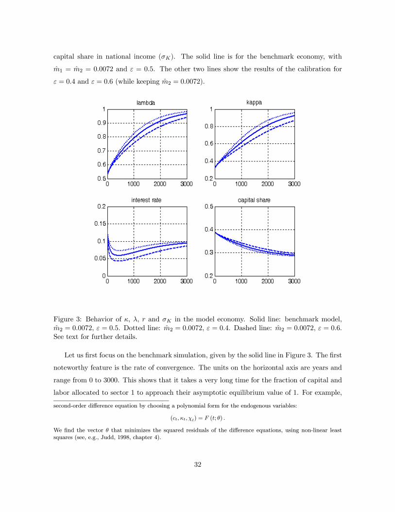
capital share in national income (σK). The solid line is for the benchmark economy, with

m1 = m2 = 0.0072 and ε = 0.5. The other two lines show the results of the calibration for

ε = 0.4 and ε = 0.6 (while keeping m2 = 0.0072).

Figure 3: Behavior of κ, λ, r and σK in the model economy. Solid line: benchmark model,m2 = 0.0072, ε = 0.5. Dotted line: m2 = 0.0072, ε = 0.4. Dashed line: m2 = 0.0072, ε = 0.6.See text for further details.

Let us first focus on the benchmark simulation, given by the solid line in Figure 3. The first

noteworthy feature is the rate of convergence. The units on the horizontal axis are years and

range from 0 to 3000. This shows that it takes a very long time for the fraction of capital and

labor allocated to sector 1 to approach their asymptotic equilibrium value of 1. For example,

second-order difference equation by choosing a polynomial form for the endogenous variables:

(ct, κt, χt) = F (t; θ) .

We find the vector θ that minimizes the squared residuals of the difference equations, using non-linear leastsquares (see, e.g., Judd, 1998, chapter 4).

32

initially, about 52% of employment is in sector 1, and after 500 years, this number has increased

only to about 70%. The implied allocation of capital between the two sectors is a similar. This

illustrates that even though in the limiting equilibrium one of the sectors employs all of the

factors, it takes a very long time for the economy to approach this limit point. Second, the

rental rate of capital (or the interest rate) follows a non-monotonic pattern, but does not vary

by much (remaining between 6% and 10% for most of the 3000 years). Third, the share of

capital in national income is declining visibly. As noted above, this is by construction, since

the initial capital share is set as σK (0) = 0.39, while the model implies that the asymptotic

capital share is σ∗K = 0.28. More importantly, the decline of the capital share is relatively

slow.

These patterns can be seen most clearly in Table 1, which shows US data from 1948 to 2004

for the relative (real) output and employment of the high and low capital intensity sectors and

the capital share in national income (see Appendix B) as well as the results from the calibration

of the model for the same time period. In particular, since t = 0 for the calibration is taken to

be 1948, the implied numbers for 2004 are given by the calibration for the time period t = 56.

The first two columns of this table confirm the pattern shown in Figure 2 in the Introduction;

real output grows faster in high capital intensity sectors, while employment grows faster in

low capital intensity sectors. The next two columns show that the benchmark calibration is

consistent with this pattern, though the magnitude of changes is somewhat smaller in the

calibration than in the data. For example, Y2/Y1 increases by about 25% in the data between

1948 and 2004, while the increase is about 15% in the benchmark calibration. Similarly, L2/L1

declines by about 33% in the data, while the implied decline in the model is about 12%.20

The movements of the capital share in national income, on the other hand, are similar in both

cases. In the data there is a decline from 0.41 to 0.39 between 1948 and 2004, whereas in

the model there is a slightly smaller decline from 0.39 to 0.38. These results suggest that our

model economy generates changes in the relative output and employment of the two sectors

that are quantitatively as well as qualitatively plausible, even though the magnitudes of the

changes are about half as large as those in the data.

20Note that the initial values of Y2/Y1 and L2/L1 (and λ) are not the same in the data and in the benchmarkmodel, since, as explained above, we chose the sectoral allocation of labor implied by the model given the relativenominal outputs of the two sectors (recall equation (60)).

33

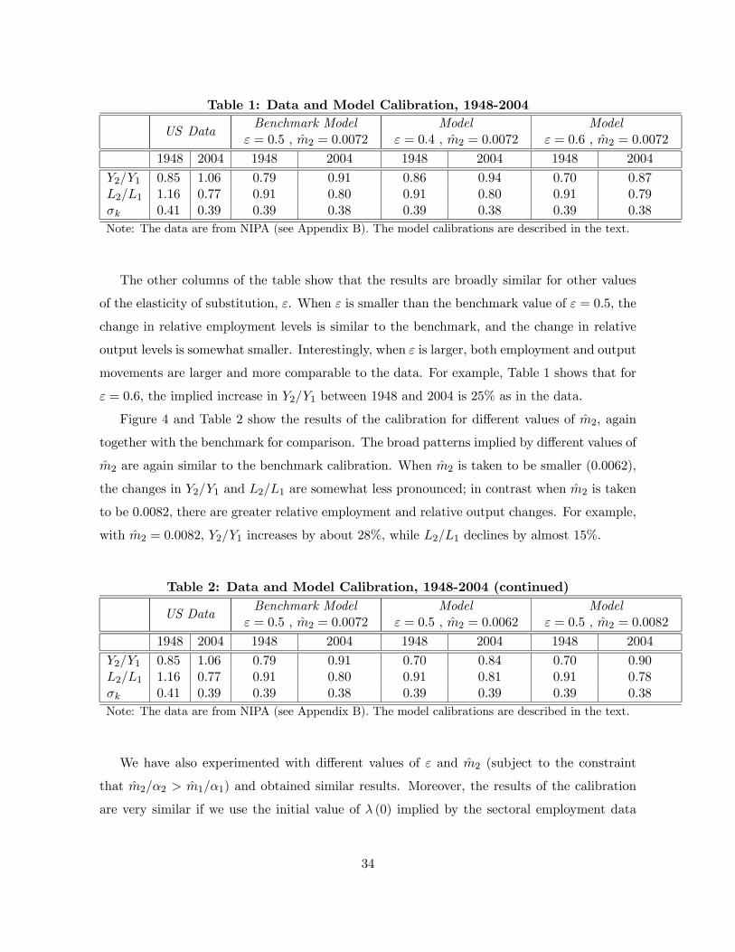
Table 1: Data and Model Calibration, 1948-2004

US DataBenchmark Model

ε = 0.5 , m2 = 0.0072Model

ε = 0.4 , m2 = 0.0072Model

ε = 0.6 , m2 = 0.0072

1948 2004 1948 2004 1948 2004 1948 2004

Y2/Y1 0.85 1.06 0.79 0.91 0.86 0.94 0.70 0.87L2/L1 1.16 0.77 0.91 0.80 0.91 0.80 0.91 0.79σk 0.41 0.39 0.39 0.38 0.39 0.38 0.39 0.38

Note: The data are from NIPA (see Appendix B). The model calibrations are described in the text.

The other columns of the table show that the results are broadly similar for other values

of the elasticity of substitution, ε. When ε is smaller than the benchmark value of ε = 0.5, the

change in relative employment levels is similar to the benchmark, and the change in relative

output levels is somewhat smaller. Interestingly, when ε is larger, both employment and output

movements are larger and more comparable to the data. For example, Table 1 shows that for

ε = 0.6, the implied increase in Y2/Y1 between 1948 and 2004 is 25% as in the data.

Figure 4 and Table 2 show the results of the calibration for different values of m2, again

together with the benchmark for comparison. The broad patterns implied by different values of

m2 are again similar to the benchmark calibration. When m2 is taken to be smaller (0.0062),

the changes in Y2/Y1 and L2/L1 are somewhat less pronounced; in contrast when m2 is taken

to be 0.0082, there are greater relative employment and relative output changes. For example,

with m2 = 0.0082, Y2/Y1 increases by about 28%, while L2/L1 declines by almost 15%.

Table 2: Data and Model Calibration, 1948-2004 (continued)

US DataBenchmark Model

ε = 0.5 , m2 = 0.0072Model

ε = 0.5 , m2 = 0.0062Model

ε = 0.5 , m2 = 0.0082

1948 2004 1948 2004 1948 2004 1948 2004

Y2/Y1 0.85 1.06 0.79 0.91 0.70 0.84 0.70 0.90L2/L1 1.16 0.77 0.91 0.80 0.91 0.81 0.91 0.78σk 0.41 0.39 0.39 0.38 0.39 0.39 0.39 0.38

Note: The data are from NIPA (see Appendix B). The model calibrations are described in the text.

We have also experimented with different values of ε and m2 (subject to the constraint

that m2/α2 > m1/α1) and obtained similar results. Moreover, the results of the calibration

are very similar if we use the initial value of λ (0) implied by the sectoral employment data

34

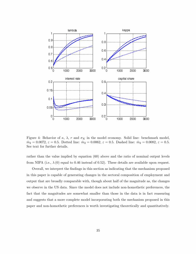
Figure 4: Behavior of κ, λ, r and σK in the model economy. Solid line: benchmark model,m2 = 0.0072, ε = 0.5. Dotted line: m2 = 0.0062, ε = 0.5. Dashed line: m2 = 0.0082, ε = 0.5.See text for further details.

rather than the value implied by equation (60) above and the ratio of nominal output levels

from NIPA (i.e., λ (0) equal to 0.46 instead of 0.52). These details are available upon request.

Overall, we interpret the findings in this section as indicating that the mechanism proposed

in this paper is capable of generating changes in the sectoral composition of employment and

output that are broadly comparable with, though about half of the magnitude as, the changes

we observe in the US data. Since the model does not include non-homothetic preferences, the

fact that the magnitudes are somewhat smaller than those in the data is in fact reassuring

and suggests that a more complete model incorporating both the mechanism proposed in this

paper and non-homothetic preferences is worth investigating theoretically and quantitatively.

35

5 Non-Balanced Endogenous Growth

In this section we introduce endogenous technological progress. This investigation has two

objectives. As already emphasized, non-balanced growth results from capital deepening, and so

far, capital deepening was a consequence of exogenous technological change. The first question

is whether endogenous technological change might restore balanced growth. The analysis in

this section will show that this is not the case. Second, endogenizing technological change in

this context enables us to derive a model of non-balanced endogenous technological change,

which is an important direction for models of endogenous technology, given the non-balanced

nature of growth in the data. In particular, we will see that differences in capital intensity

between sectors naturally lead to non-balanced endogenous technological progress.

Demographics, preferences and technology are the same as described in Section 3, with two

differences. First, instead of the exogenous processes for technology given in (21), we now need

to specify an innovation possibilities frontier, i.e., the technology to transform resources into

blueprints for new varieties in the two sectors. We assume that

M1 = b1M−ϕ1 X1 and M2 = b2M

−ϕ2 X2, (61)

where X1 ≥ 0 and X2 ≥ 0 are research expenditures in terms of the final good, b1 and b2 are

strictly positive constants measuring the technical difficulty of creating new blueprints in the

two sectors, and ϕ ∈ (−1,∞) measures the degree of spillovers in technology creation.21

Second, we assume that firms that invent blueprints for intermediates in either sector

become the monopolist supplier of that intermediate, with a fully-enforced perpetual patent.

There is free entry into research, which means that any firm can make use of the innovation

possibilities frontier (61) in order to invent new varieties.

The value of the monopolist for intermediate i in sector s is given by

Vs(i, t) =

Z ∞

texp

∙−Z v

tr(z)dz

¸πs(i, v)dv, (62)

21When ϕ = 0, there are no spillovers from the current stock of knowledge to future innovations. With ϕ < 0,there are positive spillovers and the stock of knowledge in a particular sector makes further innovation in thatsector easier. With ϕ > 0, there are negative spillovers (“fishing out”) and further innovations are more difficultin sectors that are more advanced (see, for example, Jones, 1995, Kortum, 1997). Similar to the results in Jones(1995), Young (1999) and Howitt (1999), there will be endogenous growth for a range of values of ϕ becauseof population growth. In the remainder, we will typically think of ϕ > 0, so that there are negative spillovers,though this is not important for any of the asymptotic results.Also, this innovation possibilities frontier assumes that only the final good is used to generate new technologies.

The alternative is to have a scarce factor, such as labor or scientists, in which case some amount of positivespillovers would be necessary to generate endogenous growth.

36

for s = 1, 2, where πs (i, t) = (qs (i, t)−mcs (i, t)) ys (i, t) is the flow profits for firm i at time

t, with qs given by the iso-elastic demand curves in (23) in Section 3, and mcs is the marginal

cost of production in this sector, which was also defined in Section 3. In equilibrium, all firms

in the same sector will make the same profits, so Vs(i, t) = Vs(t), and we use V1(t) and V2(t)

to denote the values of firms in the two sectors at time t.

Each monopolist chooses its price to maximize (62). Since demands are iso-elastic and

prices at time t only influence revenues and costs at that point, profit-maximizing prices will

be given by a constant markup over marginal cost:

q1(i) =

µν

ν − 1

¶α1 (1− α1)

α1−1 r1−α1wα1 , (63)

q2(i) =

µν

ν − 1

¶α2 (1− α2)

α2−1 r1−α2wα2 . (64)

These prices are identical to the intermediate prices in Section 3, (24) and (25), except for

the presence of the markup terms, ν/ (ν − 1). Now, combining equations (22), (23), (26) and(27) from Section 3 (which all still apply in the endogenous growth economy), the prices for

the labor- and capital-intensive intermediates can be expressed as q1 = γM1

ν−11 (Y1/Y )

− 1ε and

q2 = (1− γ)M1

ν−12 (Y2/Y )

− 1ε . These prices combined again with (26) and (27) and the fact

that there is a markup of ν/ (ν − 1) over marginal costs enable us to write the flow profits

from the sale of the labor- and capital-intensive intermediates as:

π1 =γ

ν

µY1Y

¶−1ε Y1

M1and π2 =

1− γ

ν

µY2Y

¶− 1ε Y2M2

. (65)

Because of the markups, factor prices are also slightly different in this section than in

Section 3. In particular, we have:

w =

µν − 1ν

¶γα1

µY

Y1

¶1ε Y1L1

and w =

µν − 1ν

¶(1− γ)α2

µY

Y2

¶1ε Y2L2

, (66)

r =

µν − 1ν

¶γ (1− α1)

µY

Y1

¶ 1ε Y1K1

and r =

µν − 1ν

¶(1− γ) (1− α2)

µY

Y2

¶1ε Y2K2

. (67)

Even though factor prices include the markup term (ν − 1) /ν, this markup is the same in bothsectors. Consequently, the allocation of capital in labor between the two sectors is unchanged

and is still determined by equations (33) and (34) in Section 3.

Given the value for being the monopolist for intermediate in (62), the free entry conditions

take the following form:

V1 ≤Mϕ1

b1and V2 ≤

Mϕ2

b2, (68)

37

with each condition holding as equality when there is positive R&D expenditure for that sector,

i.e., when X1 > 0 or X2 > 0.

The resource constraint of the economy is also modified to incorporate the R&D expendi-

tures becomes

K +C +X1 +X2 ≤ Y. (69)

Finally, the problem of consumer optimization is similar to that in Section 3. In particular,

the Euler equation is still given by (43), but the transversality condition needs to be modified

because of corporate profits. The financial wealth of the representative consumer now comes

from payments to capital and profits and is thus given by W (t) = K (t) + M1 (t)V1 (t) +

M2 (t)V2 (t), where recall that V1 (t) is the present discounted value of the profits of a firm in

the sector 1 at time t and there are M1 (t) such firms, and similarly for V2 (t) and M2 (t). The

relevant transversality condition can then be written as

limt→∞

W (t) exp

µ−Z t

0r (τ) dτ

¶= 0. (70)

Definition 5 A dynamic equilibrium is given by paths of wages and interest rates, w and

r, labor and capital allocation decisions, λ and κ, satisfying (33), (34), (66) and (67), and of

consumption C, employment, L, capital stock,K, technology,M1 andM2 values of innovation,

V1 and V2, and research expenditures, X1 and X2, satisfying (12), (43), (61), (62), (68), (69)

and (70).

It is also useful to define a path that satisfies all of these equations, possibly except the

transversality condition, (70), as a quasi-equilibrium.

Since the case with ε < 1 is both more interesting, and in view of the discussion in footnote

5, also more realistic, in this section we focus on this case exclusively.

We first note that Propositions 1 and 2 from Section 3 still apply and characterize the

comparative static responses. Moreover, Lemmas 1 and 2 from Section 3 continue to determine

the behavior of the growth rate of sectoral output, capital and employment. For the analysis

of the economy with endogenous technology, we also need an additional result in the next

lemma. It shows that provided that (i) ε < 1, (ii) there exists a constant asymptotic interest

rate r∗ (i.e., limt→∞ r = 0), and (iii) there is positive population growth, in the asymptotic

equilibrium the free entry conditions in (68) will both hold as equality:

38

Lemma 3 Suppose that ε < 1, n > 0, and limt→∞ r = 0, then limt→∞ (V1 −Mϕ1 /b1) = 0 and

limt→∞ (V2 −Mϕ2 /b2) = 0.

Proof. See Appendix A.

This lemma is an important result for the analysis of non-balanced endogenous growth. It

implies that both free-entry conditions must hold as equalities in the limiting equilibrium and

thus enables us to solve for the asymptotic growth rates from the free entry conditions and

obtain a relatively simple characterization of the constant growth path equilibrium.

The economic intuition for the lemma comes from population growth; with population

growth, it is always optimal to allocate more capital to each sector, which increases the prof-

itability of intermediate producers in that sector. Consequently, the value of a new blueprint

increases asymptotically. This rules out asymptotic equilibrium paths with slack free-entry

conditions, because along such paths, the cost of creating a new blueprint would remain con-

stant, ultimately violating the free-entry condition.

To establish the existence of a CGP, we now impose the following parameter restriction,

which replaces (A2) in the exogenous technology case:

α1ζ > 1 and ρ > (1− θ)α1ζ

α1ζ − 1n, (A3)

where ζ ≡ (ν − 1) (1 + ϕ). Assumption A3 ensures that the transversality condition (70)

holds. Notice that in contrast to Assumption A2 only α1 features in this condition; this is

because Assumption A1 already imposed that α1 < α2, and with endogenous technology, this

is sufficient to make sector 1 the more slowly growing sector in the asymptotic equilibrium.

Assumption A3 also rules out quasi-equilibrium paths where output and consumption grow

more than exponentially. This is stated in the next lemma.

Lemma 4 Suppose Assumption A3 holds and ε < 1, then there exists no quasi-equilibria with

limt→∞ C/C =∞.

This lemma is also proved in Appendix A, where, for completeness, we also show that

Assumption A3 is “tight” in the sense that, if first inequality in this assumption did not

hold, there always exist quasi-equilibria with more than exponential growth (which would also

naturally violate the transversality condition). The proof of this lemma also makes clear that

the second part of Assumption A3 is also necessary for the transversality condition.

39

Lemmas 3 and 4 together imply that the asymptotic equilibrium has to converge either

to a limit with constant growth of consumption, or to a limit cycle. Using these results, the

next theorem establishes the existence of a unique constant growth path, with non-balanced

sectoral growth, but constant share of capital and constant interest rate in the aggregate. This

theorem is therefore the analogue of Theorem 3 in Section 3.

Theorem 5 Suppose Assumptions A1 and A3 hold, ε < 1, and n > 0, then there exists a

unique CGP where

g∗ = g∗C = g∗1 = z∗1 =α1ζ

α1ζ − 1n, (71)

g∗2 =α1ζ (1− ε+ ζ) + εζ (α1 − α2)

(α1ζ − 1) (1− ε+ ζ)n > g∗, (72)

z∗2 =α1ζ (1− ε+ ζ)− ζ (α1 − α2) (1− ε)

(α1ζ − 1) (1− ε+ ζ)n < g∗, (73)

n∗1 = n and n∗2 =

∙1− ζ (1− ε) (α1 − α2)

(α1ζ − 1) [1− ε+ ζ]

¸n, (74)

m∗1 =1

1 + ϕz∗1 and m∗2 =

1

1 + ϕz∗2 . (75)

Proof. See Appendix A.

A number of features are worth noting. First, this theorem shows that the equilibrium of

this non-balanced endogenous growth economy takes a relatively simple form. Second, given

the equilibrium rates of technological change in the two sectors, m∗1 and m∗2, the asymptotic

growth rates are identical to those in Theorem 3 in Section 3, so that the economy with

endogenous technological change gives the same insights as the one with exogenous technology.

In particular, there is non-balanced sectoral growth, but in the aggregate, the economy has a

limiting equilibrium with constant share of capital in national income and a constant interest

rate.

Finally and interestingly, technology is also endogenously non-balanced, and in fact, tries

to counteract the non-balanced nature of economic growth. Specifically, there is more tech-

nological change towards the sector that is growing more slowly (recall we are focusing on

the case where ε < 1), so that the sector with lower capital intensity employs an increasing

share of the capital and labor in the economy and over time has access to increasingly superior

technology. Nevertheless, this sector still grows more slowly than the more capital-intensive

sector, and the non-balanced nature of the growth process remains. Therefore, endogenous

40

growth does not restore balance between the two sectors as long as capital intensity (factor

proportion) differences between the two sectors remain.

Unfortunately, we do not have an equivalent of Theorem 4 for the endogenous growth

economy. The reason is that there are two more endogenous state variables and two more

control variables now, so the dynamical system includes c, χ, κ, M1, M2, X1 and X2 (or

their stationary transformations). Given the size of this system, we are unable to prove local

(saddle-path) stability. Nevertheless, Lemmas 3 and 4 imply that the system cannot lead to

an explosive path, thus it has two tend to a constant growth path or settle into a limit cycle.

6 Conclusions

This paper shows how differences in factor proportions across sectors combined with capital

deepening lead to a non-balanced pattern of economic growth. We first illustrated this point

using a general two-sector growth model, and then characterized the equilibrium fully using a

class of economies with constant elasticity of substitution between sectors and Cobb-Douglas

production technologies. This class of economies shows how the pattern of equilibrium may

be consistent with both non-balanced sectoral growth and the aggregate Kaldor facts, in par-

ticular, approximately constant share of capital in national income and interest rates. We

also constructed and analyzed a model with endogenous technology featuring non-balanced

economic growth.

The main contribution of the paper is theoretical, demonstrating that the interaction

between capital deepening and factor proportion differences across sectors will lead to non-

balanced growth, while still remaining consistent with the aggregate Kaldor facts. We also

presented a simple calibration of our baseline model, which showed that the equilibrium path

may indeed exhibit sectoral employment and output shares changing significantly, while the

aggregate capital share and the interest rate remain approximately constant. Moreover, the

magnitudes implied by this simple calibration are comparable to, though somewhat smaller

than, the sectoral changes observed in the the postwar US data. A full investigation of whether

the mechanism suggested in this paper is first-order in practice is an empirical question left

for future research. It would be particularly useful to combine the mechanism proposed in this

paper with non-homothetic preferences and estimate a structural version of the model with

multiple sectors using US or OECD data.

41

7 Appendix A: Proof from Section 5

7.1 Proof of Lemma 3

We will prove this lemma in four steps.Step 1: m∗1 = m∗2 = 0 imply g

∗2 = g∗1 = n.

Step 2: lim supt→∞ (V1 −Mϕ1 /b1) ≥ 0 or lim supt→∞ (V2 −Mϕ

2 /b2) ≥ 0.Step 3: lim supt→∞ (V1 −Mϕ

1 /b1) ≥ 0 and lim supt→∞ (V2 −Mϕ2 /b2) ≥ 0.

Step 4: limt→∞ (V1 −Mϕ1 /b1) = 0 and limt→∞ (V2 −Mϕ

2 /b2) = 0.

Proof of Step 1: We first prove that m∗1 = m∗2 = 0 imply g∗2 = g∗1 = n. To see this, combineequations (31) and (32) to obtainµ

Y2Y1

¶ 1−εε

=

µ1− γ

γ

¶µ1− α21− α1

¶K1

K2.

Differentiating gives

1− ε

ε(α2n2 − α1n1) +

1− ε

ε(1− α2) z2 −

1− ε

ε(1− α1) z1 = z1 − z2. (76)

To derive a contradiction, suppose that g∗2 > g∗1 . Differentiating (27), we obtain

g1 = α1n1 + (1− α1) z1 +1

ν − 1m1 and g2 = α2n2 + (1− α2) z2 +1

ν − 1m2. (77)

Then, from Lemma 1 n∗2 < n∗1 and z∗2 < z∗1 and from Lemma 2, g∗ = g∗1 . Since limt→∞ r = 0, equation(46) and the fact that g∗ = g∗1 imply that g

∗1 = z∗1 . This combined with equation (77) and m∗1 = 0

implies that z∗1 = n∗1 = n, which together with (76) implies

0 >1− ε

ε(1− α2) (z

∗2 − z∗1) > z∗1 − z∗2 ,

yielding a contradiction. The argument for the case in which g∗2 < g∗1 is analogous. Since g∗2 = g∗1 = g∗

and m∗1 = m∗2 = 0, it must also be the case that g∗2 = g∗1 = n, completing the proof of step 1.

Proof of Step 2: First note that lim supt→∞ (V1 −Mϕ1 /b1) < 0 and

lim supt→∞ (V2 −Mϕ2 /b2) < 0 imply that the free entry conditions, (68), are asymptotically slack, so

m∗1 and m∗2 exist, and limt→∞m1 (t) = m∗1 = 0 and limt→∞m2 (t) = m∗2 = 0 (since they cannot benegative). In particular, note that if lim supt→∞ (V1 −Mϕ

1 /b1) < 0, this implies that there exists no“infinitely-recurring” interval in the limit where the free entry condition holds for sector 1.

Now to derive a contradiction, suppose that m∗2 = m∗1 = 0, which, as shown above, implies g∗1 =g∗2 = g∗ = n > 0. Then, differentiating the second equation in (65), we obtain:

limt→∞

π2π2= g∗ > 0. (78)

Combining this with limt→∞ r = 0 and the value function in (62) yields: limt→∞ V2 = ∞. Sincem∗2 = 0 by hypothesis, M−ϕ2 is constant, and we have limt→∞ V2 = ∞ > limt→∞Mϕ

2 /b2, violat-ing the free entry condition (68). This proves that m∗1 and m∗2 cannot both equal to 0, and thuslim supt→∞ (V2 −Mϕ

2 /b2) < 0 and lim supt→∞ (V1 −Mϕ1 /b1) < 0 is not possible.

Proof of Step 3: We next prove that lim supt→∞ (V1 −Mϕ1 /b1) ≥ 0,

lim supt→∞ (V2 −Mϕ2 /b2) ≥ 0, lim supt→∞m1 > 0 and lim supt→∞m2 > 0.

42

Suppose, to derive a contradiction, lim supt→∞m2 = m∗2 = 0 andlim supt→∞ (V2 −Mϕ

2 /b2) < 0 (the other case is proved analogously). Since, as shown above, m∗1 =m∗2 = 0 is not possible, we must have lim supt→∞ (V1 −Mϕ

1 /b1) ≥ 0 and lim supt→∞m1 > 0.We start by noting from (65), that asymptotically

limt→∞

π2π2=1

ε(g − g2) + g2, (79)

because m∗2 = 0. Since

limt→∞

r

r=1

ε(g − g2) + g2 − z2 = 0

from (32), z2 > 0 implies that limt→∞ π2/π2 > 0. But by the same argument as in Step 2, we havelimt→∞ V2 = ∞ > limt→∞Mϕ

2 /b2, violating the free entry condition (68). We therefore only haveto show that z2 > 0 (which would naturally imply that lim supt→∞ z2 > 0). Suppose, to obtain acontradiction, that z∗2 = 0. Using (45) and (46) from the proof of Lemma 1, we have z2−n2 = z1−n1,which implies that n∗2 = 0 (recall that either n1 ≥ n or n2 ≥ n, and since limt→∞ g ≥ n, eitherz1 ≥ n or z2 ≥ n). But then with n∗2 = z∗2 = m∗2 = 0, we have g∗2 = 0 < g∗1 , which contradictsn∗2 < n∗1 = n from Lemma 1. A similar argument for the other sector completes the proof thatlim supt→∞ (V1 −Mϕ

1 /b1) ≥ 0 and lim supt→∞ (V2 −Mϕ2 /b2) ≥ 0.

Proof of Step 4. From the free entry conditions in (68), we have that V1 −Mϕ1 /b1 ≤ 0 and

V2 −Mϕ2 /b2 ≤ 0, thus lim supt→∞ (V1 −Mϕ

1 /b1) ≤ 0 and lim supt→∞ (V2 −Mϕ2 /b2) ≤ 0. Combined

with Step 3, this implies lim supt→∞ (V1 −Mϕ1 /b1) = 0 and

lim supt→∞ (V2 −Mϕ2 /b2) = 0. Hence, we only have to prove that lim inft→∞ (V1 −Mϕ

1 /b1) ≥ 0 andlim inft→∞ (V2 −Mϕ

2 /b2) ≥ 0. We prove the first inequality (the proof of the second is similar).Suppose, to derive a contradiction, that lim inft→∞ (V1 −Mϕ

1 /b1) < 0. This implies that there existsa (recurring) interval (t00, t

02) such that V1 (t)−Mϕ

1 (t) /b1 < 0 for all t ∈ (t00, t02). Suppose that (t00, t02)is unbounded; this would imply that lim supt→∞m1 = m∗1 = 0, yielding a contradiction with Step2. Thus (t00, t

02) must be bounded, so there exists (t0, t2) ⊃ (t00, t02) such that for t ∈ (t0, t2) \ (t00, t02),

we have V1 (t) − Mϕ1 (t) /b1 = 0. Moreover, since lim supt→∞m1 > 0, there also exists an interval

(t000 , t002) ⊃ (t0, t2) such that for all t ∈ (t0, t2) \ (t000 , t002), m1 > 0.Next, since m1 = 0 for all t ∈ (t00, t02), we also have M1 (t

00) =M1 (t

02). This implies

V1 (t02) =

Mϕ1 (t

00)

b1= V1 (t

00) . (80)

Figure A1 shows this diagrammatically.Let us rewrite (62) in the Bellman equation form

V1 (t)

r= V1 (t)−

π1 (t)

r∀t. (81)

Equation (81) also shows that V1 (t) is well-defined, so V1 (t) is continuously differetiable in t. Equation(80) and the fact that V1 (t)−Mϕ

1 (t00) /b1 < 0 for all t ∈ (t00, t02) imply that V1 (t) reaches a minimum

over (t00, t02) with V1 (t) = 0. Let t

01 < t02 be such that V1 (t

01) is the first local minimum after t00, which

naturally satisfies V1 (t01) < V1 (t

00). Moreover, using (65) and (67), we have that for all t

π1 (t)

r∗=

1

(ν − 1) (1− α1)

K1 (t)

M1 (t),

where r∗ = limt→∞ r (t) is the asymptotic equilibrium interest rate, which exists by hypothesis thatlimt→∞ r (t) = 0. Also, using the fact that limt→∞ r (t) = 0 and the interest rate equation, (67), we

43

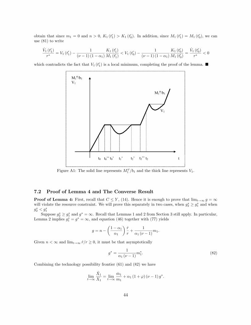
obtain that since m1 = 0 and n > 0, K1 (t01) > K1 (t

00). In addition, since M1 (t

01) = M1 (t

00), we can

use (81) to write

V1 (t01)

r∗= V1 (t

01)−

1

(ν − 1) (1− α1)

K1 (t01)

M1 (t01)< V1 (t

00)−

1

(ν − 1) (1− α1)

K1 (t00)

M1 (t00)=

V1 (t00)

r∗< 0

which contradicts the fact that V1 (t01) is a local minimum, completing the proof of the lemma. ¥

V1

M1φ/b1

t

M1φ/b1

V1

t0’’ t1’ t0’ t2’ t2’’

t0 t2

Figure A1: The solid line represents Mϕ1 /b1 and the thick line represents V1.

7.2 Proof of Lemma 4 and The Converse Result

Proof of Lemma 4: First, recall that C ≤ Y , (14). Hence it is enough to prove that limt→∞ g =∞will violate the resource constraint. We will prove this separately in two cases, when g∗2 ≥ g∗1 and wheng∗2 < g∗1

Suppose g∗2 ≥ g∗1 and g∗ =∞. Recall that Lemmas 1 and 2 from Section 3 still apply. In particular,

Lemma 2 implies g∗1 = g∗ =∞, and equation (46) together with (77) yields

g = n−µ1− α1α1

¶r

r+

1

α1 (ν − 1)m1.

Given n <∞ and limt→∞ r/r ≥ 0, it must be that asymptotically

g∗ =1

α1 (ν − 1)m∗1. (82)

Combining the technology possibility frontier (61) and (82) we have

limt→∞

X1

X1= lim

t→∞

m1

m1+ α1 (1 + ϕ) (ν − 1) g∗.

44

Then, the first inequality in Assumption A3, ζ > 1/α1, implies

limt→∞

X1

X1> g∗,

which violates the resource constraint (69).Next suppose that g∗1 > g∗2and g∗ = ∞. Then, following the same steps above, Lemma 2 implies

g∗2 = g∗ =∞, and equation (46) together with (45) and (77) yieldsµ1− α1 (1− ε)

ε

¶g1 = α1n1 +

µ1− α1

ε

¶g − (1− α1)

r

r+

µ1

ν − 1

¶m1.

Since g∗ =∞ , a fortiori g∗1 =∞, and, given n <∞ and limt→∞ r/r ≥ 0, we have that asymptotically

m∗1 = (ν − 1)∙µ1− α1 (1− ε)

ε

¶g∗1 −

µ1− α1

ε

¶g∗¸. (83)

Once again the innovation possibilities frontier (61) implies

limt→∞

X1

X1= lim

t→∞

m1

m1+ α1 (1− ϕ)m∗1.

Then equation (83) together with the first inequality in Assumption A3, ζ > 1/α1, implies

limt→∞

X1

X1> α1 (1− ϕ) (ν − 1) g∗ > g∗,

which violates the resource constraint (69), completing the proof that when Assumption A3 holds, anyquasi-equilibrium with more than exponential growth violates the resource constraint. ¥

For completeness, we also prove the converse of Lemma 4, which shows that the use of the firstinequality in Assumption A3, ζ > 1/α1, in this lemma is “tight” in the sense that, if it were relaxed,the opposite result would obtain.

Lemma 4’: Suppose A1 holds, but ζ ≡ (ν − 1) (1− ϕ) ≤ 1/α1, then there exists quasi-equilibriawith limt→∞ g =∞.

Proof. This lemma will be proved by showing that in this case

g∗2 = g∗1 = g∗ =∞ and z∗2 = z∗1 = z∗ (84)

z∗ = g∗ − r

r(85)

m1

m1=

m2

m2= [1− α1ζ] g (86)

is a quasi-equilibrium.Combining equation (46) from Section 3 with (84), we obtain

z∗ = g∗ − limt→∞

r

r

which is exactly condition (85). By substituting into (77), we obtain

g∗ = n1 −µ1− α1α1

¶limt→∞

r

r+

1

α1 (ν − 1)m∗1

45

g∗ = n2 −µ1− α2α2

¶limt→∞

r

r+

1

α2 (ν − 1)m∗2

which gives g∗ = 1α1(ν−1)m

∗1 and g∗ = 1

α2(ν−1)m∗2, and hence

m∗1 =α1α2

m∗2.

Differentiating this condition gives the first equality of equation (86).Next, from the technology possibilities frontiers, (61), feasibility requires

limt→∞

X1

X1=

m∗1m∗1

+ α1ζg∗ ≤ g∗

limt→∞

X2

X2=

m∗2m∗2

+ α2ζg∗ ≤ g∗

and both these conditions are satisfied given the second equality of equation (86) and α1 > α2.

7.3 Proof of Theorem 5

We prove this proposition in two steps.Step 1: Provided that g∗2 ≥ g∗1 > 0, then there exists a unique CGP defined by equations (71),

(72), (73), (74) and (75), satisfying g∗2 > g∗1 > 0.Step 2: All CGP must satisfy g∗2 ≥ g∗1 > 0.

Proof of Step 1. Lemma 3 establishes that as t→∞ the free-entry conditions (68) must asymp-totically hold as equality. Combining (68) as equality with (81) (and the equivalent for sector 2), weobtain the following conditions that must hold as t→∞:

γν

¡Y1Y

¢− 1ε Y1

r − ϕm1=

M1+ϕ1

b1and

γν

¡Y2Y

¢− 1ε Y2

r − ϕm2=

M1+ϕ2

b2(87)

Differentiating (87) yields:

g1 −1

ε(g1 − g)− (1 + ϕ)m1 = 0 and g2 −

1

ε(g2 − g)− (1 + ϕ)m2 = 0. (88)

Then g∗2 > g∗1 > 0 and Lemma 2 imply that we must also have g∗ = g∗1 . This condition together oursystem of equations, (45), (46), (77), (88), solves uniquely for n∗1, n

∗2, z

∗1 , z

∗2 , m

∗1, m

∗2, g

∗1 and g∗2 (and

κ∗ = λ∗ = 1) as given in equations (71), (72), (73), (74) and (75). Note that this solution is consistentwith g∗2 > g∗1 > 0, since Assumptions A1 and A3 immediately imply that g∗2 > g∗1 and g∗1 > 0 (whichis also consistent with Lemma 3). Finally, C ≤ Y , (14) and (44) imply that the consumption growthrate, g∗C , is equal to the growth rate of output, g

∗.Finally, we can verify that an equilibrium with κ∗, λ∗, n∗1, n

∗2, z

∗1 , z

∗2 , m

∗1, m

∗2, g

∗1 and g∗2 satisfies

the transversality condition (44) with a similar argument to the one spelled in the first step of the proofof Theorem 3 (since Assumption A3 ensures that g∗ < r∗).

Proof of Step 2. The proof that along all CGPs g∗2 > g∗1 > 0 must be true, is analogous to theone of the second step in the proof of Theorem 3. ¥

46

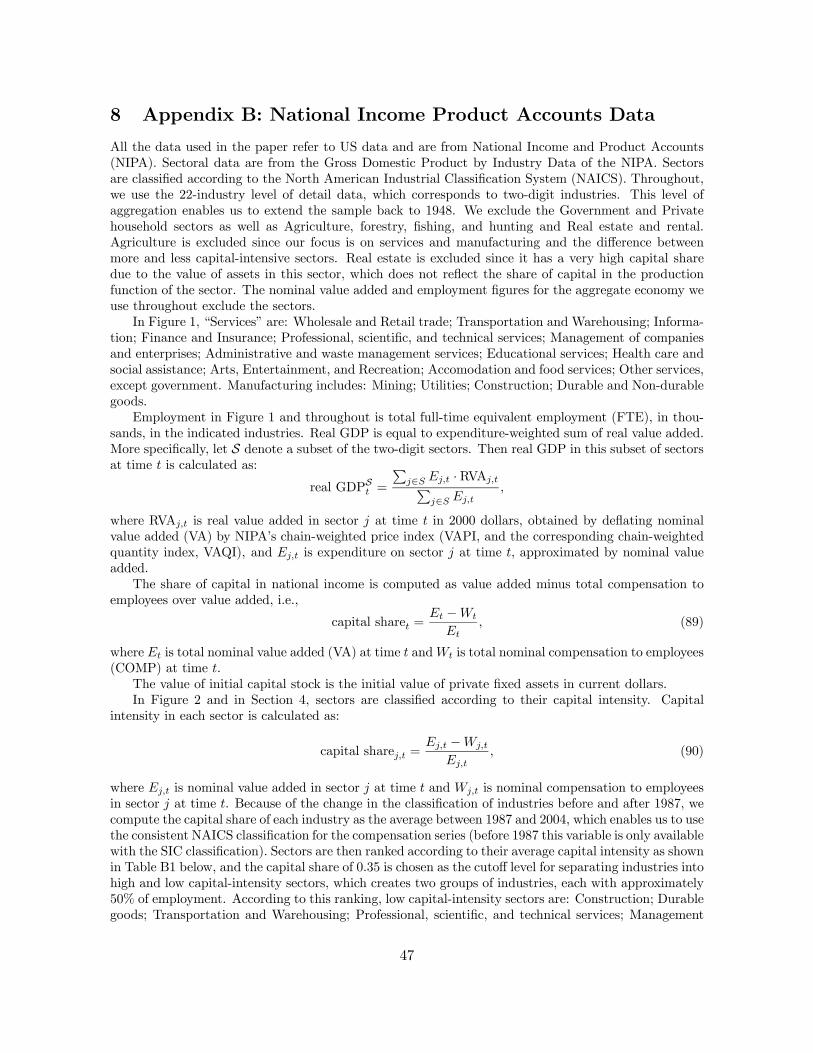
8 Appendix B: National Income Product Accounts Data

All the data used in the paper refer to US data and are from National Income and Product Accounts(NIPA). Sectoral data are from the Gross Domestic Product by Industry Data of the NIPA. Sectorsare classified according to the North American Industrial Classification System (NAICS). Throughout,we use the 22-industry level of detail data, which corresponds to two-digit industries. This level ofaggregation enables us to extend the sample back to 1948. We exclude the Government and Privatehousehold sectors as well as Agriculture, forestry, fishing, and hunting and Real estate and rental.Agriculture is excluded since our focus is on services and manufacturing and the difference betweenmore and less capital-intensive sectors. Real estate is excluded since it has a very high capital sharedue to the value of assets in this sector, which does not reflect the share of capital in the productionfunction of the sector. The nominal value added and employment figures for the aggregate economy weuse throughout exclude the sectors.

In Figure 1, “Services” are: Wholesale and Retail trade; Transportation and Warehousing; Informa-tion; Finance and Insurance; Professional, scientific, and technical services; Management of companiesand enterprises; Administrative and waste management services; Educational services; Health care andsocial assistance; Arts, Entertainment, and Recreation; Accomodation and food services; Other services,except government. Manufacturing includes: Mining; Utilities; Construction; Durable and Non-durablegoods.

Employment in Figure 1 and throughout is total full-time equivalent employment (FTE), in thou-sands, in the indicated industries. Real GDP is equal to expenditure-weighted sum of real value added.More specifically, let S denote a subset of the two-digit sectors. Then real GDP in this subset of sectorsat time t is calculated as:

real GDPSt =

Pj∈S Ej,t ·RVAj,tP

j∈S Ej,t,

where RVAj,t is real value added in sector j at time t in 2000 dollars, obtained by deflating nominalvalue added (VA) by NIPA’s chain-weighted price index (VAPI, and the corresponding chain-weightedquantity index, VAQI), and Ej,t is expenditure on sector j at time t, approximated by nominal valueadded.

The share of capital in national income is computed as value added minus total compensation toemployees over value added, i.e.,

capital sharet =Et −Wt

Et, (89)

where Et is total nominal value added (VA) at time t andWt is total nominal compensation to employees(COMP) at time t.

The value of initial capital stock is the initial value of private fixed assets in current dollars.In Figure 2 and in Section 4, sectors are classified according to their capital intensity. Capital

intensity in each sector is calculated as:

capital sharej,t =Ej,t −Wj,t

Ej,t, (90)

where Ej,t is nominal value added in sector j at time t and Wj,t is nominal compensation to employeesin sector j at time t. Because of the change in the classification of industries before and after 1987, wecompute the capital share of each industry as the average between 1987 and 2004, which enables us to usethe consistent NAICS classification for the compensation series (before 1987 this variable is only availablewith the SIC classification). Sectors are then ranked according to their average capital intensity as shownin Table B1 below, and the capital share of 0.35 is chosen as the cutoff level for separating industries intohigh and low capital-intensity sectors, which creates two groups of industries, each with approximately50% of employment. According to this ranking, low capital-intensity sectors are: Construction; Durablegoods; Transportation and Warehousing; Professional, scientific, and technical services; Management

47

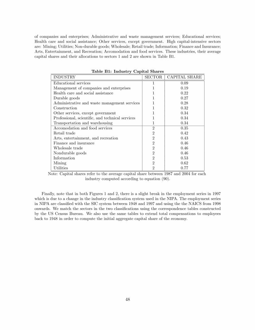
of companies and enterprises; Administrative and waste management services; Educational services;Health care and social assistance; Other services, except government. High capital-intensive sectorsare: Mining; Utilities; Non-durable goods; Wholesale; Retail trade; Information; Finance and Insurance;Arts, Entertainment, and Recreation; Accomodation and food services. These industries, their averagecapital shares and their allocations to sectors 1 and 2 are shown in Table B1.

Table B1: Industry Capital Shares

INDUSTRY SECTOR CAPITAL SHARE

Educational services 1 0.09Management of companies and enterprises 1 0.19Health care and social assistance 1 0.22Durable goods 1 0.27Administrative and waste management services 1 0.28Construction 1 0.32Other services, except government 1 0.34Professional, scientific, and technical services 1 0.34Transportation and warehousing 1 0.34Accomodation and food services 2 0.35Retail trade 2 0.42Arts, entertainment, and recreation 2 0.43Finance and insurance 2 0.46Wholesale trade 2 0.46Nondurable goods 2 0.46Information 2 0.53Mining 2 0.62Utilities 2 0.77

Note: Capital shares refer to the average capital share between 1987 and 2004 for eachindustry computed according to equation (90).

Finally, note that in both Figures 1 and 2, there is a slight break in the employment series in 1997which is due to a change in the industry classification system used in the NIPA. The employment seriesin NIPA are classified with the SIC system between 1948 and 1997 and using the the NAICS from 1998onwards. We match the sectors in the two classifications using the correspondence tables constructedby the US Census Bureau. We also use the same tables to extend total compensations to employeesback to 1948 in order to compute the initial aggregate capital share of the economy.

48

References

[1] Acemoglu, Daron, “Directed Technical Change” Review of Economic Studies, LXIX

(2002), 781-810.

[2] Acemoglu, Daron, “Labor- and Capital-Augmenting Technical Change” Journal of Euro-

pean Economic Association, I (2003), 1-37.

[3] Aghion, Philippe and Peter Howitt, “A Model of Growth Through Creative Destruction”

Econometrica, LX (1992), 323-351.

[4] Aghion, Philippe and Peter Howitt, Endogenous Growth Theory, Cambridge, MA, MIT

Press, 1998.

[5] Antras, Pol, “Is the U.S. Aggregate Production Function Cobb-Douglas? New Estimates

of the Elasticity of Substitution” MIT mimeo (2001).

[6] Barro, Robert and Xavier Sala-i-Martin. Economic Growth, McGraw Hill, New York

(2004, 2nd edition).

[7] Baumol, William J., “Macroeconomics of Unbalanced Growth: The Anatomy of Urban

Crisis”, American Economic Review, LVII (1967), 415-426.

[8] Berndt, Ernst, “Reconciling Alternative Estimates of the Elasticity of Substitution,” Re-

view of Economics and Statistics, LVIII (1976), 59-68.

[9] Bewley, Truman, “An Integration of Equilibrium Theory and Turnpike Theory” Journal

of Mathematical Economics, X (1982), 233-267.

[10] Buera, Francisco and Joseph Kaboski “The Rise of the Service Economy” Northwestern

mimeo, 2006.

[11] Caselli, Francesco and John Coleman, “The U. S. Structural Transformation and Regional

Convergence: a Reinterpretation” Journal of Political Economy CIX (2001) 584-617.

[12] Chenery, Hollis, “Patterns of Industrial Growth”, American Economic Review, V (1960),

624-654.

49

[13] Chirinko, Robert S. “Business Fixed Investment: a Critical Survey of Modeling Strategies,

Empirical Results and Policy Implications” Journal of Economic Literature, XXXI, (1993),

1875-1911.

[14] Chirinko, Robert S., Steven M. Fazzari and Andrew P. Mayer, “How Responsive Is Busi-

ness Capital Formation to Its User Cost?” Journal of Public Economics, LXXV, (1999),

53-80.

[15] David, Paul, and Th. Van de Klundert, “Biased Efficiency Growth and Capital-Labor

Substitution in the U.S., 1899-1960,” American Economic Review, LV, (1965), 357-393.

[16] Denison, Edward F, “Accounting for United States Economic Growth, 1929-1969” Wash-

ington, DC: Brookings Institution (1974).

[17] Echevarria, Cristina, “Changes in Sectoral Composition Associated with Economic

Growth”, International Economic Review, XXXVIII (1997), 431-452.

[18] Foellmi, Reto and Josef Zweimuller “Structural Change and the Kaldor Facts of Economic

Growth” CEPR Discussion Paper, No. 3300, 2002.

[19] Gollin, Douglas, Stephen Parente and Richard Rogerson “The Role of Agriculture in

Development” American Economic Review Papers and Proceedings XCII (2002) 160-164.

[20] Griffin, James M. and Paul R. Gregory, “An Intercountry Translog Model of Energy

Substitution Responses”, American Economic Review, LXVI (1976), 845-857.

[21] Grossman, Gene and Elhanan Helpman, “Quality Ladders in the Theory of Growth”

Review of Economic Studies, LIIX (1991a), 43-61.

[22] Grossman, Gene and Elhanan Helpman, Innovation and Growth in the Global Economy,

Cambridge, MA, MIT Press, 1991b.

[23] Hall, Robert E. and Charles I. Jones “The Value of Life and the Rise in Health Spending”

forthcoming Quarterly Journal of Economics, (2006).

[24] Hamermesh, David S., Labor Demand, Princeton University Press, Princeton 1993.

[25] Homer, Sydney and Richard Sylla A History of Interest Rates, Rutgers University Press,

New Brunswick, 1991.

50

[26] Howitt, Peter, “Steady Endogenous Growth with Population and R&D Inputs Growing”

Journal of Political Economics, CVII (1999), 715-730.

[27] Jensen, Martin K. “Balanced Growth, Dynamic Stability and the Turnpike” University

of Copenhagen, Ph.D. dissertation, 2002.

[28] Jones, Charles I., “R&D-Based Models of Economic Growth”, Journal of Political Eco-

nomics, CIII (1995), 759-784.

[29] Jones, Charles I., “The Shape of Production Functions and the Direction of Technical

Change”, U.C. Berkeley mimeo (2004).

[30] Judd, Kenneth, Numerical Methods in Economics, MIT Press, Cambridge, 1998.

[31] Kaldor, Nicholas , “Capital Accumulation and Economic Growth”, in Friedrich A. Lutz

and Douglas C. Hague, eds., Proceedings of a Conference Held by the International Eco-

nomics Association, London, Macmillan.(1963)

[32] Kongsamut, Piyabha , Sergio Rebelo and Danyang Xie, “Beyond Balanced Growth”,

Review of Economic Studies, LXVIII (2001), 869-882.

[33] Kortum, Samuel, “Research, Patenting and Technological Change” Econometrica, LXV

(1997), 1389-1431.

[34] Krusell, Per; Lee Ohanian and Victor Rios-Rull and Giovanni Violante, “Capital Skill

Complementary and Inequality”, Econometrica, LXIIX (2000), 1029-1053.

[35] Kuznets, Simon, “Quantitative Aspects of the Economic Growth of Nations: II, Indus-

trial Distribution of National Product and Labour Forcce”, Economic Development and

Cultural Change, V Supplement (1957).

[36] Kuznets, Simon, “Modern Economic Growth: Findings and Reflections”, American Eco-

nomic Review, LXIII (1973), 829-846.

[37] Laitner, John, “Structural Change and Economic Growth”, Review of Economic Studies,

LXVII (2000), 545-561.

[38] Lucas, Robert E., “On the mechanics of economic development.” Journal of Monetary

Economics, XXII (1988), 3-42.

51

[39] Matsuyama, Kiminori, “Agricultural Productivity, Comparative Advantage and Economic

Growth” Journal of Economic Theory LVIII (1992), 317-334.

[40] Matsuyama, Kiminori, “The Rise of Mass Consumption Societies” Journal of Political

Economy, CX (2002), 1093-1120.

[41] Matsuyama, Kiminori, “Structural Change” forthcoming New Pelgrave Dictionary of Eco-

nomics (2005).

[42] Mairesse, Jacques, Bronwyn H. Hall and Benoit Mulkay, “Firm-Level Investment in France

and the United States: An Exploration over What We Have Returned in Twenty Years”

Annales d’Economie et Statistiques, LV (1999), 27-67.

[43] McKenzie, Lionel W., “Turnpikes: Richard Ely Lecture” American Economic Review,

(1998).

[44] Murphy, Kevin, Andrei Shleifer and Robert Vishny, “Income Distribution, Market Size

and Industrialization” Quarterly Journal of Economics CIV (1989), 537-564.

[45] Nadiri, M. I. “Some Approaches to Theory and Measurement of Total Factor Productivity:

a Survey” Journal of Economic Literature, VIII, (1970), 1117-77.

[46] Nerlove, Mark, “Recent Empirical Studies of the CES and Related Production Functions”

in M. Brown (editor) The Theory and Empirical Analysis of Production New York (1967).

[47] Ngai Rachel and Christopher Pissarides, “Structural Change in a Multi-Sector Model of

Growth”, London School of Economics, mimeo, 2006.

[48] Radner, Roy “Paths of Economic Growth That Are Optimal With Regard Only to Final

States” Review of Economic Studies, XXVIII (1961), 98-104.

[49] Romer, Paul M., “Increasing Returns and Long-Run Growth” Journal of Political Econ-

omy, XCIV (1986), 1002-1037.

[50] Romer, Paul M., “Endogenous Technological Change” Journal of Political Economy, IIC

(1990), S71-S102.

[51] Rybczynski, Tadeusz, “Factor Endowments and Relative Commodity Prices” Economica,

XXII (1955), 336-341.

52

[52] Scheinkman, Jose A. “On Optimal Steady States of n-Sector Growth Models When Utility

Is Discounted” Journal of Economic Theory, XII (1976), 11-20.

[53] Segerstrom, Paul S., T. C. A. Anant, and Elias Dinopoulos, “A Schumpeterian Model of

the Product Life Cycle” American Economic Review LXXX (1990), 1077-1092.

[54] Stokey, Nancy “Learning by Doing in the Introduction of New Goods” Journal of Political

Economy, XCVI (1988), 701-717.

[55] Stokey, Nancy, “Human Capital, Product Quality and Growth” Quarterly Journal of

Economics, CVI (1991), 587-616.

[56] Young, Alwyn “Invention and Bounded Learning by Doing” Journal of Political Economy

CI (1993), 443-472.

[57] Young, Alwyn “Growth without Scale Effect” Journal of Political Economy, CVI (1998),

41-63.

[58] Zuleta, Hernando and Andrew Young “Labor’s Shares–Aggregate and Industry: Ac-

counting for Both in a Model with Induced Innovation” University of Mississippi, mimeo,

2006.

53