1 / 142 From Joins to Aggregates and Optimization Problems: One idea to rule them all and at their core factorize them! Dan Olteanu (Oxford) http://www.cs.ox.ac.uk/projects/FDB/ RiSE & LogiCS Summer School, July 4, 2017

Welcome message from author
This document is posted to help you gain knowledge. Please leave a comment to let me know what you think about it! Share it to your friends and learn new things together.
Transcript

1 / 142
From Joins to Aggregates and Optimization Problems:
One idea to rule them all and at their core factorize them!
Dan Olteanu (Oxford)
http://www.cs.ox.ac.uk/projects/FDB/
RiSE & LogiCS Summer School, July 4, 2017
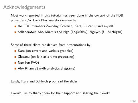
Acknowledgements
Most work reported in this tutorial has been done in the context of the FDB
project and/or LogicBlox analytics engine by
the FDB members Zavodny, Schleich, Kara, Ciucanu, and myself
collaborators Abo Khamis and Ngo (LogicBlox), Nguyen (U. Michigan)
Some of these slides are derived from presentations by
Kara (on covers and various graphics)
Ciucanu (on join-at-a-time processing)
Ngo (on FAQ)
Abo Khamis (in-db analytics diagrams)
Lastly, Kara and Schleich proofread the slides.
I would like to thank them for their support and sharing their work!
2 / 142
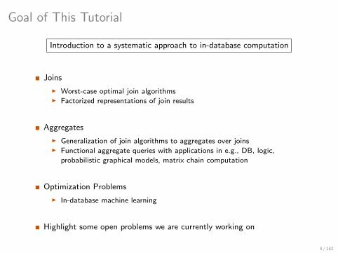
Goal of This Tutorial
Introduction to a systematic approach to in-database computation
Joins
I Worst-case optimal join algorithmsI Factorized representations of join results
Aggregates
I Generalization of join algorithms to aggregates over joinsI Functional aggregate queries with applications in e.g., DB, logic,
probabilistic graphical models, matrix chain computation
Optimization Problems
I In-database machine learning
Highlight some open problems we are currently working on
3 / 142
Part 1. Joins
Part 2. Aggregates
Part 3. Optimization
Part 4. Open Problems
4 / 142
Outline
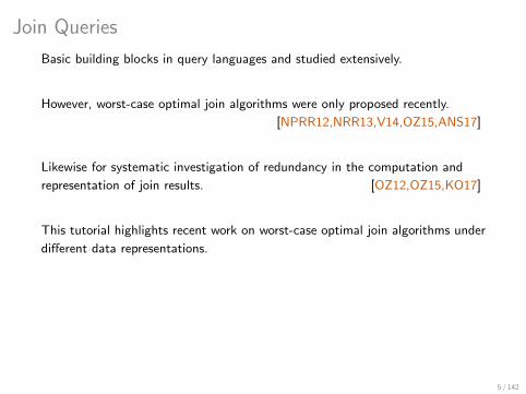
Join Queries
Basic building blocks in query languages and studied extensively.
However, worst-case optimal join algorithms were only proposed recently.
[NPRR12,NRR13,V14,OZ15,ANS17]
Likewise for systematic investigation of redundancy in the computation and
representation of join results. [OZ12,OZ15,KO17]
This tutorial highlights recent work on worst-case optimal join algorithms under
different data representations.
5 / 142
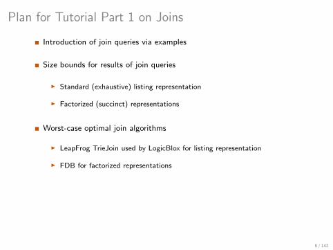
Plan for Tutorial Part 1 on Joins
Introduction of join queries via examples
Size bounds for results of join queries
I Standard (exhaustive) listing representation
I Factorized (succinct) representations
Worst-case optimal join algorithms
I LeapFrog TrieJoin used by LogicBlox for listing representation
I FDB for factorized representations
6 / 142

Introduction to Join Queries
7 / 142
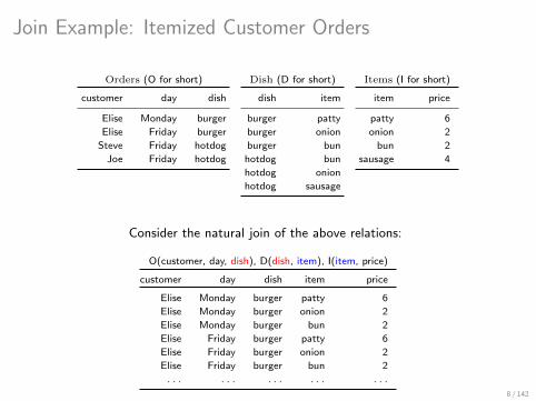
Join Example: Itemized Customer Orders
Orders (O for short)
customer day dish
Elise Monday burger
Elise Friday burger
Steve Friday hotdog
Joe Friday hotdog
Dish (D for short)
dish item
burger patty
burger onion
burger bun
hotdog bun
hotdog onion
hotdog sausage
Items (I for short)
item price
patty 6
onion 2
bun 2
sausage 4
Consider the natural join of the above relations:
O(customer, day, dish), D(dish, item), I(item, price)
customer day dish item price
Elise Monday burger patty 6
Elise Monday burger onion 2
Elise Monday burger bun 2
Elise Friday burger patty 6
Elise Friday burger onion 2
Elise Friday burger bun 2
. . . . . . . . . . . . . . .
8 / 142
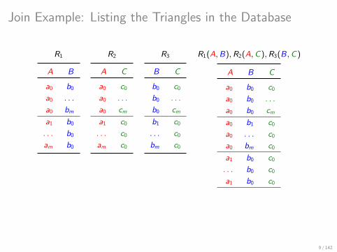
Join Example: Listing the Triangles in the Database
R1 R2 R3 R1(A,B),R2(A,C),R3(B,C)
A B
a0 b0
a0 . . .
a0 bm
a1 b0
. . . b0
am b0
A C
a0 c0
a0 . . .
a0 cm
a1 c0
. . . c0
am c0
B C
b0 c0
b0 . . .
b0 cm
b1 c0
. . . c0
bm c0
A B C
a0 b0 c0
a0 b0 . . .
a0 b0 cm
a0 b1 c0
a0 . . . c0
a0 bm c0
a1 b0 c0
. . . b0 c0
a1 b0 c0
9 / 142
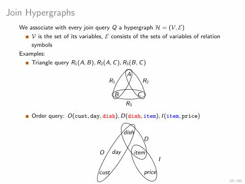
Join Hypergraphs
We associate with every join query Q a hypergraph H = (V, E)
V is the set of its variables, E consists of the sets of variables of relation
symbols
Examples:
Triangle query R1(A,B),R2(A,C),R3(B,C)
R1 R2
R3
A
B C
Order query: O(cust, day, dish),D(dish, item), I (item, price)
O
D
I
dish
day item
cust price
10 / 142
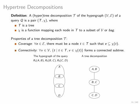
Hypertree Decompositions
Definition: A (hyper)tree decomposition T of the hypergraph (V, E) of a
query Q is a pair (T , χ), where
T is a tree
χ is a function mapping each node in T to a subset of V or bag.
Properties of a tree decomposition T :
Coverage: ∀e ∈ E , there must be a node t ∈ T such that e ⊆ χ(t).
Connectivity: ∀v ∈ V, t | t ∈ T , v ∈ χ(t) forms a connected subtree.
The hypergraph of the query
R1(A,B),R2(B,C),R3(C ,D)
A tree decomposition
A
B
C
D
A,B
B,C
C ,D
11 / 142
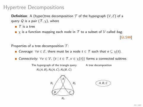
Hypertree Decompositions
Definition: A (hyper)tree decomposition T of the hypergraph (V, E) of a
query Q is a pair (T , χ), where
T is a tree
χ is a function mapping each node in T to a subset of V called bag.
[GLS99]
Properties of a tree decomposition T :
Coverage: ∀e ∈ E , there must be a node t ∈ T such that e ⊆ χ(t).
Connectivity: ∀v ∈ V, t | t ∈ T , v ∈ χ(t) forms a connected subtree.
The hypergraph of the triangle query
R1(A,B),R2(A,C),R3(B,C)
A tree decomposition
R1 R2
R3
A
B C
A,B,C
12 / 142
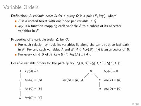
Variable Orders
Definition: A variable order ∆ for a query Q is a pair (F , key), where
F is a rooted forest with one node per variable in Q
key is a function mapping each variable A to a subset of its ancestor
variables in F .
Properties of a variable order ∆ for Q:
For each relation symbol, its variables lie along the same root-to-leaf path
in F . For any such variables A and B, A ∈ key(B) if A is an ancestor of B.
For every child B of A, key(B) ⊆ key(A) ∪ A.
Possible variable orders for the path query R1(A,B),R2(B,C),R3(C ,D):
A
B
C
D
key(A) = ∅
key(B) = A
key(C) = B
key(D) = C
B
A C
D
key(B) = ∅
key(C) = B
key(D) = C
key(A) = B
13 / 142
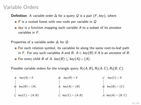
Variable Orders
Definition: A variable order ∆ for a query Q is a pair (F , key), where
F is a rooted forest with one node per variable in Q
key is a function mapping each variable A to a subset of its ancestor
variables in F .
Properties of a variable order ∆ for Q:
For each relation symbol, its variables lie along the same root-to-leaf path
in F . For any such variables A and B, A ∈ key(B) if A is an ancestor of B.
For every child B of A, key(B) ⊆ key(A) ∪ A.
Possible variable orders for the triangle query R1(A,B),R2(A,C),R3(B,C):
A
B
C
key(A) = ∅
key(B) = A
key(C) = A,B
B
A
C
key(B) = ∅
key(A) = B
key(C) = A,B
C
B
A
key(C) = ∅
key(B) = C
key(A) = B,C
14 / 142
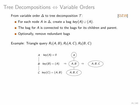
Tree Decompositions ⇔ Variable Orders
From variable order ∆ to tree decomposition T : [OZ15]
For each node A in ∆, create a bag key(A) ∪ A.
The bag for A is connected to the bags for its children and parent.
Optionally, remove redundant bags
Example: Triangle query R1(A,B),R2(A,C),R3(B,C)
A
B
C
key(A) = ∅
key(B) = A
key(C) = A,B
⇒
A
A,B
A,B,C
⇒ A,B,C
15 / 142
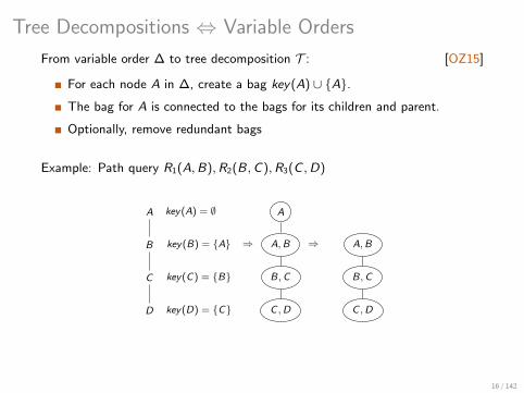
Tree Decompositions ⇔ Variable Orders
From variable order ∆ to tree decomposition T : [OZ15]
For each node A in ∆, create a bag key(A) ∪ A.
The bag for A is connected to the bags for its children and parent.
Optionally, remove redundant bags
Example: Path query R1(A,B),R2(B,C),R3(C ,D)
A
B
C
D
key(A) = ∅
key(B) = A
key(C) = B
key(D) = C
⇒
A
A,B
B,C
C ,D
⇒ A,B
B,C
C ,D
16 / 142
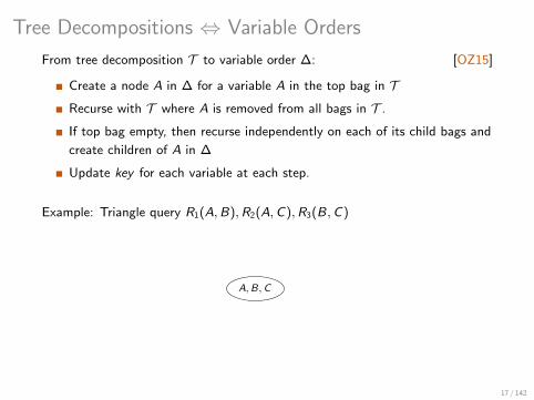
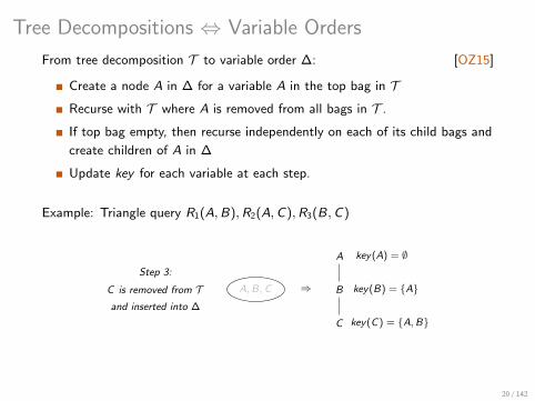
Tree Decompositions ⇔ Variable Orders
From tree decomposition T to variable order ∆: [OZ15]
Create a node A in ∆ for a variable A in the top bag in T
Recurse with T where A is removed from all bags in T .
If top bag empty, then recurse independently on each of its child bags and
create children of A in ∆
Update key for each variable at each step.
Example: Triangle query R1(A,B),R2(A,C),R3(B,C)
Step 1:
A is removed from Tand inserted into ∆
A,B,C
⇒
A
B
C
key(A) = ∅
key(B) = A
key(C) = A,B
17 / 142
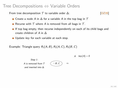
Tree Decompositions ⇔ Variable Orders
From tree decomposition T to variable order ∆: [OZ15]
Create a node A in ∆ for a variable A in the top bag in T
Recurse with T where A is removed from all bags in T .
If top bag empty, then recurse independently on each of its child bags and
create children of A in ∆
Update key for each variable at each step.
Example: Triangle query R1(A,B),R2(A,C),R3(B,C)
Step 1:
A is removed from Tand inserted into ∆
A,B,C ⇒
A
B
C
key(A) = ∅
key(B) = A
key(C) = A,B
18 / 142

Tree Decompositions ⇔ Variable Orders
From tree decomposition T to variable order ∆: [OZ15]
Create a node A in ∆ for a variable A in the top bag in T
Recurse with T where A is removed from all bags in T .
If top bag empty, then recurse independently on each of its child bags and
create children of A in ∆
Update key for each variable at each step.
Example: Triangle query R1(A,B),R2(A,C),R3(B,C)
Step 2:
B is removed from Tand inserted into ∆
A,B,C ⇒
A
B
C
key(A) = ∅
key(B) = A
key(C) = A,B
19 / 142
Tree Decompositions ⇔ Variable Orders
From tree decomposition T to variable order ∆: [OZ15]
Create a node A in ∆ for a variable A in the top bag in T
Recurse with T where A is removed from all bags in T .
If top bag empty, then recurse independently on each of its child bags and
create children of A in ∆
Update key for each variable at each step.
Example: Triangle query R1(A,B),R2(A,C),R3(B,C)
Step 3:
C is removed from Tand inserted into ∆
A,B,C ⇒
A
B
C
key(A) = ∅
key(B) = A
key(C) = A,B
20 / 142

Tree Decompositions ⇔ Variable Orders
From tree decomposition T to variable order ∆: [OZ15]
Create a node A in ∆ for a variable A in the top bag in T
Recurse with T where A is removed from all bags in T .
If top bag empty, then recurse independently on each of its child bags and
create children of A in ∆
Update key for each variable at each step.
Example: Path query R1(A,B),R2(B,C),R3(C ,D)
Step 3:
C is removed from Tand inserted into ∆
A,B
B,C
C ,D
⇒
A
B
C
D
key(A) = ∅
key(B) = A
key(C) = B
key(D) = C
21 / 142

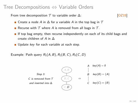
Tree Decompositions ⇔ Variable Orders
From tree decomposition T to variable order ∆: [OZ15]
Create a node A in ∆ for a variable A in the top bag in T
Recurse with T where A is removed from all bags in T .
If top bag empty, then recurse independently on each of its child bags and
create children of A in ∆
Update key for each variable at each step.
Example: Path query R1(A,B),R2(B,C),R3(C ,D)
Step 1:
A is removed from Tand inserted into ∆
A,B
B,C
C ,D
⇒
A
B
C
D
key(A) = ∅
key(B) = A
key(C) = B
key(D) = C
22 / 142
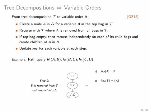
Tree Decompositions ⇔ Variable Orders
From tree decomposition T to variable order ∆: [OZ15]
Create a node A in ∆ for a variable A in the top bag in T
Recurse with T where A is removed from all bags in T .
If top bag empty, then recurse independently on each of its child bags and
create children of A in ∆
Update key for each variable at each step.
Example: Path query R1(A,B),R2(B,C),R3(C ,D)
Step 2:
B is removed from Tand inserted into ∆
A,B
B,C
C ,D
⇒
A
B
C
D
key(A) = ∅
key(B) = A
key(C) = B
key(D) = C
23 / 142
Tree Decompositions ⇔ Variable Orders
From tree decomposition T to variable order ∆: [OZ15]
Create a node A in ∆ for a variable A in the top bag in T
Recurse with T where A is removed from all bags in T .
If top bag empty, then recurse independently on each of its child bags and
create children of A in ∆
Update key for each variable at each step.
Example: Path query R1(A,B),R2(B,C),R3(C ,D)
Step 3:
C is removed from Tand inserted into ∆
A,B
B,C
C ,D
⇒
A
B
C
D
key(A) = ∅
key(B) = A
key(C) = B
key(D) = C
24 / 142
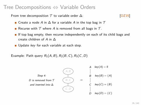
Tree Decompositions ⇔ Variable Orders
From tree decomposition T to variable order ∆: [OZ15]
Create a node A in ∆ for a variable A in the top bag in T
Recurse with T where A is removed from all bags in T .
If top bag empty, then recurse independently on each of its child bags and
create children of A in ∆
Update key for each variable at each step.
Example: Path query R1(A,B),R2(B,C),R3(C ,D)
Step 4:
D is removed from Tand inserted into ∆
A,B
B,C
C ,D
⇒
A
B
C
D
key(A) = ∅
key(B) = A
key(C) = B
key(D) = C
25 / 142

Size Bounds for Listing Representationof Join Results
26 / 142
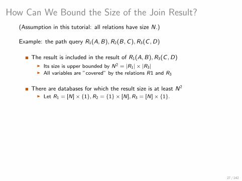
How Can We Bound the Size of the Join Result?
(Assumption in this tutorial: all relations have size N.)
Example: the path query R1(A,B),R2(B,C),R3(C ,D)
The result is included in the result of R1(A,B),R3(C ,D)
I Its size is upper bounded by N2 = |R1| × |R3|I All variables are ”covered” by the relations R1 and R3
There are databases for which the result size is at least N2
I Let R1 = [N]× 1,R2 = 1 × [N],R3 = [N]× 1.
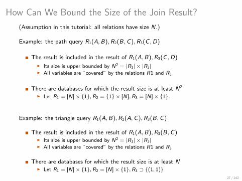
Example: the triangle query R1(A,B),R2(A,C),R3(B,C)
The result is included in the result of R1(A,B),R3(B,C)I Its size is upper bounded by N2 = |R1| × |R3|I All variables are ”covered” by the relations R1 and R3
There are databases for which the result size is at least NI Let R1 = [N]× 1,R2 = [N]× 1,R3 ⊃ (1, 1)
27 / 142
How Can We Bound the Size of the Join Result?
(Assumption in this tutorial: all relations have size N.)
Example: the path query R1(A,B),R2(B,C),R3(C ,D)
The result is included in the result of R1(A,B),R3(C ,D)
I Its size is upper bounded by N2 = |R1| × |R3|I All variables are ”covered” by the relations R1 and R3
There are databases for which the result size is at least N2
I Let R1 = [N]× 1,R2 = 1 × [N],R3 = [N]× 1.
Example: the triangle query R1(A,B),R2(A,C),R3(B,C)
The result is included in the result of R1(A,B),R3(B,C)I Its size is upper bounded by N2 = |R1| × |R3|I All variables are ”covered” by the relations R1 and R3
There are databases for which the result size is at least NI Let R1 = [N]× 1,R2 = [N]× 1,R3 ⊃ (1, 1)
27 / 142
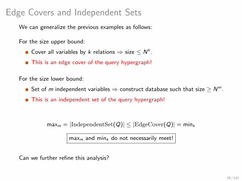
Edge Covers and Independent Sets
We can generalize the previous examples as follows:
For the size upper bound:
Cover all variables by k relations ⇒ size ≤ Nk .
This is an edge cover of the query hypergraph!
For the size lower bound:
Set of m independent variables⇒ construct database such that size ≥ Nm.
This is an independent set of the query hypergraph!
maxm = |IndependentSet(Q)| ≤ |EdgeCover(Q)| = mink
maxm and mink do not necessarily meet!
Can we further refine this analysis?
28 / 142

The Fractional Edge Cover Number ρ∗(Q)
The two bounds meet if we take their fractional versions [AGM08]
Fractional edge cover of Q with weight k ⇒ size ≤ Nk .
Fractional independent set with weight m ⇒ construct database such that
size ≥ Nm.
By duality of linear programming:
maxm = |FractionalIndependentSet(Q)| = |FractionalEdgeCover(Q)| = mink
This is the fractional edge cover number ρ∗(Q)!
29 / 142
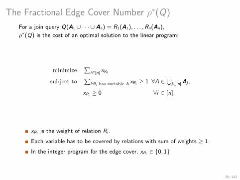
The Fractional Edge Cover Number ρ∗(Q)
For a join query Q(A1 ∪ · · · ∪ An) = R1(A1), . . . ,Rn(An),
ρ∗(Q) is the cost of an optimal solution to the linear program:
minimize∑
i∈[n] xRi
subject to∑
i :Ri has variable A xRi ≥ 1 ∀A ∈⋃
j∈[n] Aj ,
xRi ≥ 0 ∀i ∈ [n].
xRi is the weight of relation Ri .
Each variable has to be covered by relations with sum of weights ≥ 1.
In the integer program for the edge cover, xRi ∈ 0, 1
30 / 142

Example of Fractional Edge Cover Computation (1)
Consider the following join query Q:
R(A,B,C), S(A,B,D),T (A,E),U(E,F ).
A
B
C D
E
F
R
SU
T
Relations R, S ,U cover all variables.
FractionalEdgeCover(Q) ≤ 3
Each of the nodes C , D, and F must be covered by separate relations.
FractionalIndependentSet(Q) ≥ 3
⇒ ρ∗(Q) = 3
⇒ Size ≤ N3 and for some inputs is Θ(N3).31 / 142

Example of Fractional Edge Cover Computation (2)
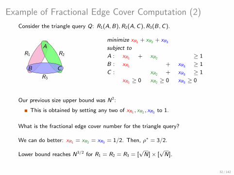
Consider the triangle query Q: R1(A,B),R2(A,C),R3(B,C).
R1 R2
R3
A
B C
minimize xR1 + xR2 + xR3
subject to
A : xR1 + xR2 ≥ 1
B : xR1 + xR3 ≥ 1
C : xR2 + xR3 ≥ 1
xR1 ≥ 0 xR2 ≥ 0 xR3 ≥ 0
Our previous size upper bound was N2:
This is obtained by setting any two of xR1 , xR2 , xR3 to 1.
What is the fractional edge cover number for the triangle query?
We can do better: xR1 = xR2 = xR3 = 1/2. Then, ρ∗ = 3/2.
Lower bound reaches N3/2 for R1 = R2 = R3 = [√N]× [
√N].
32 / 142
Example of Fractional Edge Cover Computation (2)
Consider the triangle query Q: R1(A,B),R2(A,C),R3(B,C).
R1 R2
R3
A
B C
minimize xR1 + xR2 + xR3
subject to
A : xR1 + xR2 ≥ 1
B : xR1 + xR3 ≥ 1
C : xR2 + xR3 ≥ 1
xR1 ≥ 0 xR2 ≥ 0 xR3 ≥ 0
Our previous size upper bound was N2:
This is obtained by setting any two of xR1 , xR2 , xR3 to 1.
What is the fractional edge cover number for the triangle query?
We can do better: xR1 = xR2 = xR3 = 1/2. Then, ρ∗ = 3/2.
Lower bound reaches N3/2 for R1 = R2 = R3 = [√N]× [
√N].
32 / 142
Example of Fractional Edge Cover Computation (3)
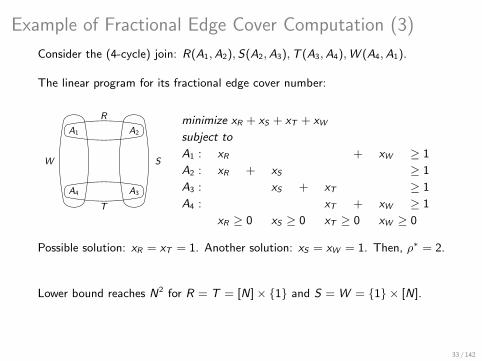
Consider the (4-cycle) join: R(A1,A2),S(A2,A3),T (A3,A4),W (A4,A1).
The linear program for its fractional edge cover number:
R
T
W S
A1 A2
A3A4
minimize xR + xS + xT + xW
subject to
A1 : xR + xW ≥ 1
A2 : xR + xS ≥ 1
A3 : xS + xT ≥ 1
A4 : xT + xW ≥ 1
xR ≥ 0 xS ≥ 0 xT ≥ 0 xW ≥ 0
Possible solution: xR = xT = 1. Another solution: xS = xW = 1. Then, ρ∗ = 2.
Lower bound reaches N2 for R = T = [N]× 1 and S = W = 1 × [N].
33 / 142
Size Bounds for Factorized Representationsof Join Results
34 / 142
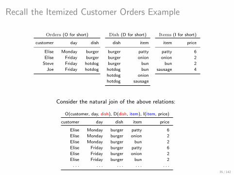
Recall the Itemized Customer Orders Example
Orders (O for short)
customer day dish
Elise Monday burger
Elise Friday burger
Steve Friday hotdog
Joe Friday hotdog
Dish (D for short)
dish item
burger patty
burger onion
burger bun
hotdog bun
hotdog onion
hotdog sausage
Items (I for short)
item price
patty 6
onion 2
bun 2
sausage 4
Consider the natural join of the above relations:
O(customer, day, dish), D(dish, item), I(item, price)
customer day dish item price
Elise Monday burger patty 6
Elise Monday burger onion 2
Elise Monday burger bun 2
Elise Friday burger patty 6
Elise Friday burger onion 2
Elise Friday burger bun 2
. . . . . . . . . . . . . . .
35 / 142

Factor Out Common Data Blocks
O(customer, day, dish), D(dish, item), I(item, price)
customer day dish item price
Elise Monday burger patty 6
Elise Monday burger onion 2
Elise Monday burger bun 2
Elise Friday burger patty 6
Elise Friday burger onion 2
Elise Friday burger bun 2
. . . . . . . . . . . . . . .
The listing representation of the above query result is:
〈Elise〉 × 〈Monday〉 × 〈burger〉 × 〈patty〉 × 〈6〉 ∪
〈Elise〉 × 〈Monday〉 × 〈burger〉 × 〈onion〉 × 〈2〉 ∪
〈Elise〉 × 〈Monday〉 × 〈burger〉 × 〈bun〉 × 〈2〉 ∪
〈Elise〉 × 〈Friday〉 × 〈burger〉 × 〈patty〉 × 〈6〉 ∪
〈Elise〉 × 〈Friday〉 × 〈burger〉 × 〈onion〉 × 〈2〉 ∪
〈Elise〉 × 〈Friday〉 × 〈burger〉 × 〈bun〉 × 〈2〉 ∪ . . .
It uses relational product (×), union (∪), and data (singleton relations).
The attribute names are not shown to avoid clutter.36 / 142
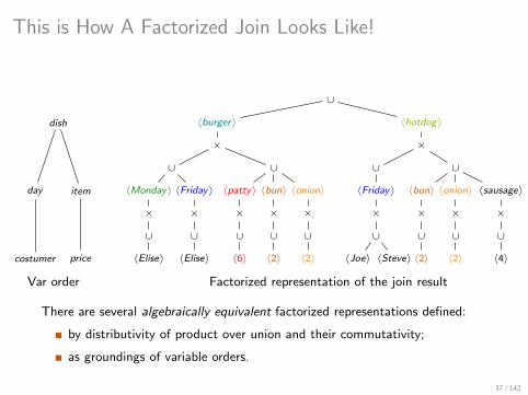
This is How A Factorized Join Looks Like!
∪
〈burger〉 〈hotdog〉
× ×
∪
〈bun〉 〈onion〉 〈sausage〉
× × ×
∪ ∪ ∪
〈2〉 〈2〉 〈4〉
∪
〈Friday〉
×
∪
〈Joe〉 〈Steve〉
∪
〈patty〉 〈bun〉 〈onion〉
× × ×
∪ ∪ ∪
〈6〉 〈2〉 〈2〉
∪
〈Friday〉
×
∪
〈Elise〉
〈Monday〉
×
∪
〈Elise〉
dish
day item
costumer price
Var order Factorized representation of the join result
There are several algebraically equivalent factorized representations defined:
by distributivity of product over union and their commutativity;
as groundings of variable orders.
37 / 142
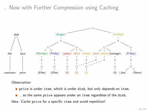
.. Now with Further Compression using Caching
∪
〈burger〉 〈hotdog〉
× ×
∪
〈sausage〉〈bun〉〈onion〉
×× ×
∪
〈4〉
∪
〈Friday〉
×
∪
〈Joe〉 〈Steve〉
∪
〈patty〉 〈bun〉 〈onion〉
× × ×
∪ ∪ ∪
〈6〉 〈2〉 〈2〉
∪
〈Friday〉
×
∪
〈Elise〉
〈Monday〉
×
∪
〈Elise〉
dish
day item
costumer price
Observation:
price is under item, which is under dish, but only depends on item,
.. so the same price appears under an item regardless of the dish.
Idea: Cache price for a specific item and avoid repetition!
38 / 142
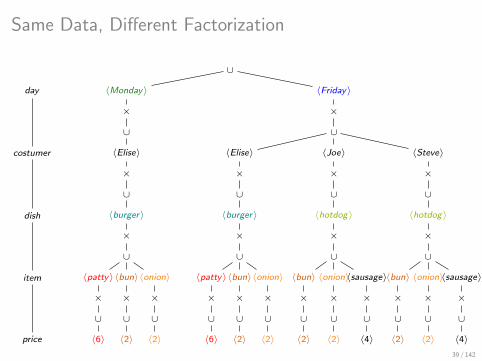
Same Data, Different Factorization
∪
〈Monday〉 〈Friday〉
× ×
∪ ∪
〈Elise〉
×
∪
〈burger〉
×
∪
〈patty〉〈bun〉〈onion〉
× × ×
∪ ∪ ∪
〈6〉 〈2〉 〈2〉
〈Elise〉
×
∪
〈burger〉
×
∪
〈patty〉〈bun〉〈onion〉
× × ×
∪ ∪ ∪
〈6〉 〈2〉 〈2〉
〈Joe〉
×
∪
〈hotdog〉
×
∪
〈bun〉 〈onion〉〈sausage〉
× × ×
∪ ∪ ∪
〈2〉 〈2〉 〈4〉
〈Steve〉
×
∪
〈hotdog〉
×
∪
〈bun〉 〈onion〉〈sausage〉
× × ×
∪ ∪ ∪
〈2〉 〈2〉 〈4〉
day
costumer
dish
item
price
39 / 142
.. and Further Compressed using Caching
∪
〈Monday〉 〈Friday〉
× ×
∪ ∪
〈Elise〉
×
∪
〈burger〉
×
∪
〈patty〉〈bun〉〈onion〉
× × ×
∪ ∪ ∪
〈6〉 〈2〉 〈2〉
〈Elise〉
×
∪
〈burger〉
×
〈Joe〉
×
∪
〈hotdog〉
×
∪
〈bun〉 〈onion〉〈sausage〉
× × ×
∪
〈4〉
〈Steve〉
×
∪
〈hotdog〉
×
day
costumer
dish
item
price
40 / 142

Which factorization should we choose?
The size of a factorization is the number of its values.
Example:
F1 =(〈1〉 ∪ · · · ∪ 〈n〉
)×(〈1〉 ∪ · · · ∪ 〈m〉
)F2 =〈1〉 × 〈1〉 ∪ · · · ∪ 〈1〉 × 〈m〉
∪ · · · ∪
〈n〉 × 〈1〉 ∪ · · · ∪ 〈n〉 × 〈m〉.
F1 is factorized, F2 is a listing representation
F1 ≡ F2
BUT |F1| = m + n |F2| = m ∗ n.
How much space does factorization save over the listing representation?
41 / 142

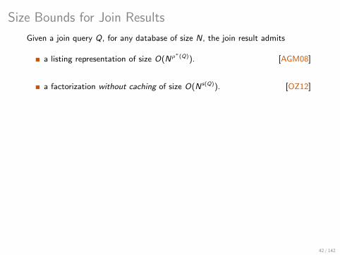
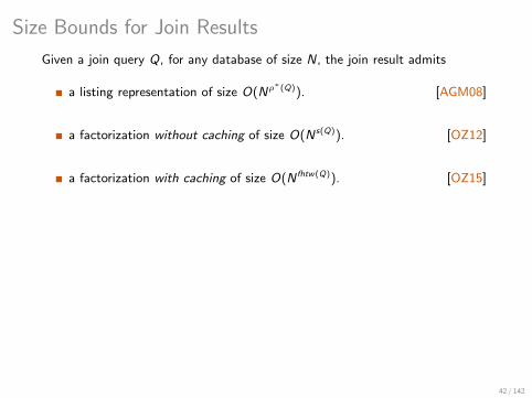
Size Bounds for Join Results
Given a join query Q, for any database of size N, the join result admits
a listing representation of size O(Nρ∗(Q)). [AGM08]
a factorization without caching of size O(Ns(Q)). [OZ12]
a factorization with caching of size O(N fhtw(Q)). [OZ15]
1 ≤ fhtw(Q) ≤︸︷︷︸up to log |Q|
s(Q) ≤︸︷︷︸up to |Q|
ρ∗(Q) ≤ |Q|
|Q| is the number of relations in Q
ρ∗(Q) is the fractional edge cover number of Q
s(Q) is the factorization width of Q
fhtw(Q) is the fractional hypertree width of Q [M10]
42 / 142

Size Bounds for Join Results
Given a join query Q, for any database of size N, the join result admits
a listing representation of size O(Nρ∗(Q)). [AGM08]
a factorization without caching of size O(Ns(Q)). [OZ12]
a factorization with caching of size O(N fhtw(Q)). [OZ15]
These size bounds are asymptotically tight!
Best possible size bounds for factorized representations over variable
orders of Q and for listing representation, but not database optimal!
There exists arbitrarily large databases for whichI the listing representation has size Ω(Nρ
∗(Q))I the factorization with (without) caching over any variable order of Q has
size Ω(Ns(Q)) (Ω(N fhtw(Q))).
43 / 142

Example: The Factorization Width s
A
B
C D
E
F
R
SU
T A
B
C D
E
F
key(A) = ∅
key(B) = A
key(C) = A,B key(D) = A,B
key(E) = A
key(F ) = E
The structure of the factorization over the above variable order ∆:⋃a∈A
(〈a〉 ×
⋃b∈B
(〈b〉 ×
( ⋃c∈C
〈c〉)×( ⋃d∈D
〈d〉))×⋃e∈E
(〈e〉 ×
( ⋃f∈F
〈f 〉)))
The number of values for a variable is dictated by the number of valid tuples of
values for its ancestors in ∆:
One value 〈f 〉 for each tuple (a, e, f ) in the join result.
Size of factorization = sum of sizes of results of subqueries along paths.
44 / 142
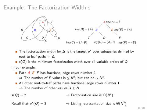
Example: The Factorization Width s
A
B
C D
E
F
R
SU
T A
B
C D
E
F
key(A) = ∅
key(B) = A
key(C) = A,B key(D) = A,B
key(E) = A
key(F ) = E
The factorization width for ∆ is the largest ρ∗ over subqueries defined by
root-to-leaf paths in ∆
s(Q) is the minimum factorization width over all variable orders of Q
In our example:
Path A–E–F has fractional edge cover number 2.
⇒ The number of F -values is ≤ N2, but can be ∼ N2.
All other root-to-leaf paths have fractional edge cover number 1.
⇒ The number of other values is ≤ N.
s(Q) = 2 ⇒ Factorization size is Θ(N2)
Recall that ρ∗(Q) = 3 ⇒ Listing representation size is Θ(N3)45 / 142

Example: The Fractional Hypertree Width fhtw
Idea: Avoid repeating identical expressions, store them once and use pointers.
A
B
C D
E
F
R
SU
T A
B
C D
E
F
key(A) = ∅
key(B) = A
key(C) = A,B key(D) = A,B
key(E) = A
key(F ) = E
⋃a∈A
[〈a〉 × · · · ×
⋃e∈E
(〈e〉 ×
( ⋃f∈F
〈f 〉))]
Observation:
Variable F only depends on E and not on A: key(F ) = E
A value 〈e〉 maps to the same union⋃
(e,f )∈U〈f 〉 regardless of its pairings
with A-values.
⇒ Define Ue =⋃
(e,f )∈U〈f 〉 for each value 〈e〉 and use Ue instead of the
union⋃
(e,f )∈U〈f 〉.
46 / 142

Example: The Fractional Hypertree Width fhtw
Idea: Avoid repeating identical expressions, store them once and use pointers.
A
B
C D
E
F
R
SU
T A
B
C D
E
F
key(A) = ∅
key(B) = A
key(C) = A,B key(D) = A,B
key(E) = A
key(F ) = E
A factorization with definitions would be:⋃a∈A
[〈a〉 × · · · ×
⋃e∈E
(〈e〉 × Ue
)];
Ue =
⋃(e,f )∈U
〈f 〉
fhtw for ∆ is the largest ρ∗(Q ′) over subqueries Q ′ defined by the
variables key(X ) ∪ X for each variable X in ∆
fhtw(Q) is the minimum fhtw over all variable orders of Q
In our example: fhtw(Q) = 1 < s(Q) = 2 < ρ∗(Q) = 3.
47 / 142
Relational Counterpartof Factorized Representation
48 / 142
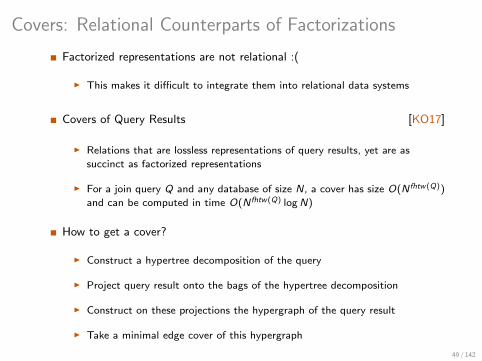
Covers: Relational Counterparts of Factorizations
Factorized representations are not relational :(
I This makes it difficult to integrate them into relational data systems
Covers of Query Results [KO17]
I Relations that are lossless representations of query results, yet are as
succinct as factorized representations
I For a join query Q and any database of size N, a cover has size O(N fhtw(Q))
and can be computed in time O(N fhtw(Q) log N)
How to get a cover?
I Construct a hypertree decomposition of the query
I Project query result onto the bags of the hypertree decomposition
I Construct on these projections the hypergraph of the query result
I Take a minimal edge cover of this hypergraph
49 / 142
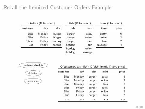
Recall the Itemized Customer Orders Example
Orders (O for short)
customer day dish
Elise Monday burger
Elise Friday burger
Steve Friday hotdog
Joe Friday hotdog
Dish (D for short)
dish item
burger patty
burger onion
burger bun
hotdog bun
hotdog onion
hotdog sausage
Items (I for short)
item price
patty 6
onion 2
bun 2
sausage 4
customer,day,dish
dish,item
item,price
O(customer, day, dish), D(dish, item), I(item, price)
customer day dish item price
Elise Monday burger patty 6
Elise Monday burger onion 2
Elise Monday burger bun 2
Elise Friday burger patty 6
Elise Friday burger onion 2
Elise Friday burger bun 2
. . . . . . . . . . . . . . .
50 / 142
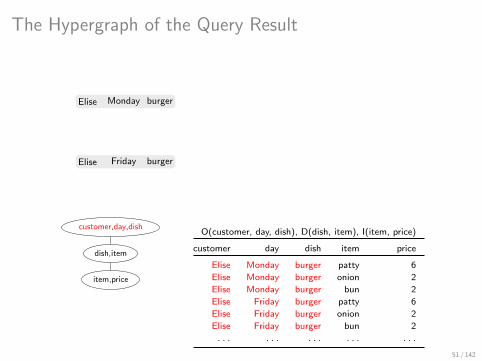
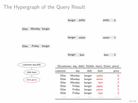
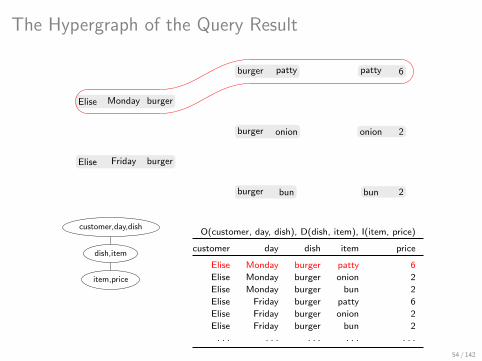
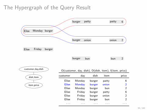
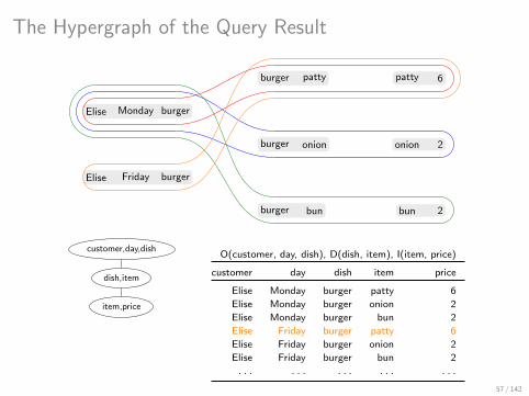
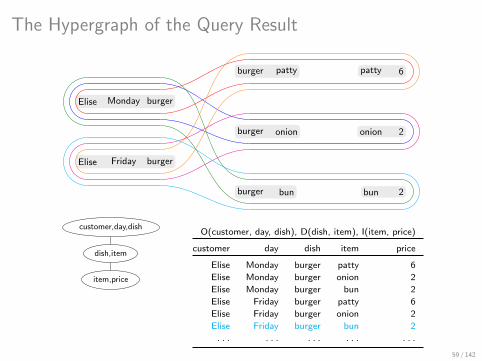
The Hypergraph of the Query Result
Elise Monday burger
Elise Friday burger
burger patty
burger onion
burger bun
patty 6
onion 2
bun 2
customer,day,dish
dish,item
item,price
O(customer, day, dish), D(dish, item), I(item, price)
customer day dish item price
Elise Monday burger patty 6
Elise Monday burger onion 2
Elise Monday burger bun 2
Elise Friday burger patty 6
Elise Friday burger onion 2
Elise Friday burger bun 2
. . . . . . . . . . . . . . .
51 / 142
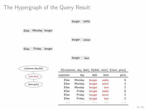
The Hypergraph of the Query Result
Elise Monday burger
Elise Friday burger
burger patty
burger onion
burger bun
patty 6
onion 2
bun 2
customer,day,dish
dish,item
item,price
O(customer, day, dish), D(dish, item), I(item, price)
customer day dish item price
Elise Monday burger patty 6
Elise Monday burger onion 2
Elise Monday burger bun 2
Elise Friday burger patty 6
Elise Friday burger onion 2
Elise Friday burger bun 2
. . . . . . . . . . . . . . .
52 / 142
The Hypergraph of the Query Result
Elise Monday burger
Elise Friday burger
burger patty
burger onion
burger bun
patty 6
onion 2
bun 2
customer,day,dish
dish,item
item,price
O(customer, day, dish), D(dish, item), I(item, price)
customer day dish item price
Elise Monday burger patty 6
Elise Monday burger onion 2
Elise Monday burger bun 2
Elise Friday burger patty 6
Elise Friday burger onion 2
Elise Friday burger bun 2
. . . . . . . . . . . . . . .
53 / 142
The Hypergraph of the Query Result
Elise Monday burger
Elise Friday burger
burger patty
burger onion
burger bun
patty 6
onion 2
bun 2
customer,day,dish
dish,item
item,price
O(customer, day, dish), D(dish, item), I(item, price)
customer day dish item price
Elise Monday burger patty 6
Elise Monday burger onion 2
Elise Monday burger bun 2
Elise Friday burger patty 6
Elise Friday burger onion 2
Elise Friday burger bun 2
. . . . . . . . . . . . . . .
54 / 142
The Hypergraph of the Query Result
Elise Monday burger
Elise Friday burger
burger patty
burger onion
burger bun
patty 6
onion 2
bun 2
customer,day,dish
dish,item
item,price
O(customer, day, dish), D(dish, item), I(item, price)
customer day dish item price
Elise Monday burger patty 6
Elise Monday burger onion 2
Elise Monday burger bun 2
Elise Friday burger patty 6
Elise Friday burger onion 2
Elise Friday burger bun 2
. . . . . . . . . . . . . . .
55 / 142

The Hypergraph of the Query Result
Elise Monday burger
Elise Friday burger
burger patty
burger onion
burger bun
patty 6
onion 2
bun 2
customer,day,dish
dish,item
item,price
O(customer, day, dish), D(dish, item), I(item, price)
customer day dish item price
Elise Monday burger patty 6
Elise Monday burger onion 2
Elise Monday burger bun 2
Elise Friday burger patty 6
Elise Friday burger onion 2
Elise Friday burger bun 2
. . . . . . . . . . . . . . .
56 / 142
The Hypergraph of the Query Result
Elise Monday burger
Elise Friday burger
burger patty
burger onion
burger bun
patty 6
onion 2
bun 2
customer,day,dish
dish,item
item,price
O(customer, day, dish), D(dish, item), I(item, price)
customer day dish item price
Elise Monday burger patty 6
Elise Monday burger onion 2
Elise Monday burger bun 2
Elise Friday burger patty 6
Elise Friday burger onion 2
Elise Friday burger bun 2
. . . . . . . . . . . . . . .
57 / 142

The Hypergraph of the Query Result
Elise Monday burger
Elise Friday burger
burger patty
burger onion
burger bun
patty 6
onion 2
bun 2
customer,day,dish
dish,item
item,price
O(customer, day, dish), D(dish, item), I(item, price)
customer day dish item price
Elise Monday burger patty 6
Elise Monday burger onion 2
Elise Monday burger bun 2
Elise Friday burger patty 6
Elise Friday burger onion 2
Elise Friday burger bun 2
. . . . . . . . . . . . . . .
58 / 142
The Hypergraph of the Query Result
Elise Monday burger
Elise Friday burger
burger patty
burger onion
burger bun
patty 6
onion 2
bun 2
customer,day,dish
dish,item
item,price
O(customer, day, dish), D(dish, item), I(item, price)
customer day dish item price
Elise Monday burger patty 6
Elise Monday burger onion 2
Elise Monday burger bun 2
Elise Friday burger patty 6
Elise Friday burger onion 2
Elise Friday burger bun 2
. . . . . . . . . . . . . . .
59 / 142
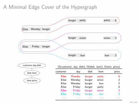
A Minimal Edge Cover of the Hypergraph
Elise Monday burger
Elise Friday burger
burger patty
burger onion
burger bun
patty 6
onion 2
bun 2
customer,day,dish
dish,item
item,price
O(customer, day, dish), D(dish, item), I(item, price)
customer day dish item price
Elise Monday burger patty 6
Elise Monday burger onion 2
Elise Monday burger bun 2
Elise Friday burger patty 6
Elise Friday burger onion 2
Elise Friday burger bun 2
. . . . . . . . . . . . . . .
60 / 142

A Cover of (a part of) the Query Result
O(customer, day, dish), D(dish, item), I(item, price)
customer day dish item price
Elise Monday burger patty 6
Elise Friday burger onion 2
Elise Friday burger bun 2
customer,day,dish
dish,item
item,price
O(customer, day, dish), D(dish, item), I(item, price)
customer day dish item price
Elise Monday burger patty 6
Elise Monday burger onion 2
Elise Monday burger bun 2
Elise Friday burger patty 6
Elise Friday burger onion 2
Elise Friday burger bun 2
. . . . . . . . . . . . . . .
61 / 142
Compression by Factorization in Practice
62 / 142
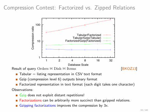
Compression Contest: Factorized vs. Zipped Relations
1
10
100
1 2 4 8 16 32
Com
pres
sion
ratio
Database Scale
Tabular/FactorizedTabular/Gzip(Tabular)
Factorized/Gzip(Factorized)
Result of query Orders 1 Dish 1 Items [BKOZ13]
Tabular = listing representation in CSV text format
Gzip (compression level 6) outputs binary format
Factorized representation in text format (each digit takes one character)
Observations:
Gzip does not exploit distant repetitions!
Factorizations can be arbitrarily more succinct than gzipped relations.
Gzipping factorizations improves the compression by 3x.63 / 142

Factorization Gains in Practice (1/3)
Retailer dataset used for LogicBlox analytics
Relations: Inventory (84M), Sales (1.5M), Clearance (368K), Promotions
(183K), Census (1K), Location (1K).
Compression factors (caching not used):
I 26.61x for natural join of Inventory, Census, Location.
I 159.59x for natural join of Inventory, Sales, Clearance, Promotions
64 / 142
Factorization Gains in Practice (2/3)
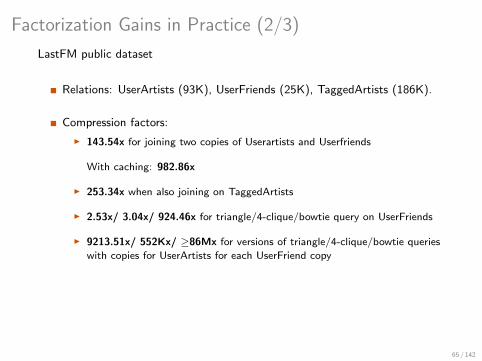
LastFM public dataset
Relations: UserArtists (93K), UserFriends (25K), TaggedArtists (186K).
Compression factors:
I 143.54x for joining two copies of Userartists and Userfriends
With caching: 982.86x
I 253.34x when also joining on TaggedArtists
I 2.53x/ 3.04x/ 924.46x for triangle/4-clique/bowtie query on UserFriends
I 9213.51x/ 552Kx/ ≥86Mx for versions of triangle/4-clique/bowtie queries
with copies for UserArtists for each UserFriend copy
65 / 142

Factorization Gains in Practice (3/3)
Twitter public dataset
Relation: Follower-Followee (1M)
Compression factors:
I 2.69x for triangle query
I 3.48x for 4-clique query
I 4918.73x for bowtie query
66 / 142
Worst-Case Optimal Join Algorithms
67 / 142

How Fast Can We Compute Join Results?
Given a join query Q, for any database of size N, the join result can be
computed in time
O(Nρ∗(Q) logN) as listing representation [NPRR12,V14]
O(Ns(Q) logN) as factorization without caching [OZ15]
O(N fhtw(Q) logN) as factorization with caching [OZ15]
These upper bounds essentially follow the succinctness gap. They are:
worst-case optimal (modulo logN) within the given representation model
with respect to data complexityI additional quadratic factor in the number of variables and linear factor in
the number of relations in Q
68 / 142

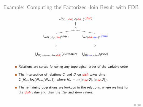
Example: Computing the Factorized Join Result with FDB
Our join: O(customer, day, dish), D(dish, item), I(item, price)
can be grounded to a factorized representation as follows:⋃O( , ,dish),D(dish, )〈dish〉
×
⋃O( ,day,dish)〈day〉
×
⋃O(customer,day,dish)〈customer〉
⋃D(dish,item)〈item〉
×
⋃I (item,price)〈price〉
This evaluation follows the variable order given below:
dish
day
customer
item
price
69 / 142
Example: Computing the Factorized Join Result with FDB
⋃O( , ,dish),D(dish, )〈dish〉
×
⋃O( ,day,dish)〈day〉
×
⋃O(customer,day,dish)〈customer〉
⋃D(dish,item)〈item〉
×
⋃I (item,price)〈price〉
Relations are sorted following any topological order of the variable order
The intersection of relations O and D on dish takes time
O(Nmin log(Nmax/Nmin)), where Nm = m(|πdishO|, |πdishD|).
The remaining operations are lookups in the relations, where we first fix
the dish value and then the day and item values.
70 / 142

LeapFrog TrieJoin
Much acclaimed worst-case optimal join algorithm used by LogicBlox [V14]
Computes a listing representation of the join result
⇒ It does not exploit factorization
Glorified multi-way sort-merge join with an efficient list intersection
LeapFrog TrieJoin (LogicBlox) is a special case of our algorithm, where
the input variable order ∆ is a path, and
for each variable A, key(A) consists of all ancestors of A in ∆.
71 / 142
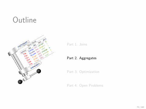
Part 1. Joins
Part 2. Aggregates
Part 3. Optimization
Part 4. Open Problems
72 / 142
Outline
Aggregates
Essential operators in any realistic query language and database-supported
application.
Much DB research into optimization of aggregates is rather ad-hoc.
Aggregates over joins can express a host of problems in Computer Science, and
it is only recently that this connection has been made explicit [ANR16]
This tutorial highlights recent theoretical work on aggregate computation with
lowest computational complexity to date [BKOZ13,ANR16]
In Part 3, we will see how this development supports state-of-the-art machine
learning inside the database [SOC16,ANNOS17]
73 / 142
Plan for Tutorial Part 2
We will first show how aggregates can be computed over factorized joins.
[BKOZ13]
We will then show how to factorize the computation of aggregates using
optimized relational queries.
We will then present a beautiful generalization of aggregates over joins
called Functional Aggregate Queries (FAQs). [ANR16]
I Captures different semirings, e.g., sum-product, max-product, Boolean
I Captures a large class of problems across Computer Science
I FAQ computation is factorized and has the computational complexity of
aggregates over factorized joins
74 / 142

Examples: Aggregates over Factorized Joins
75 / 142
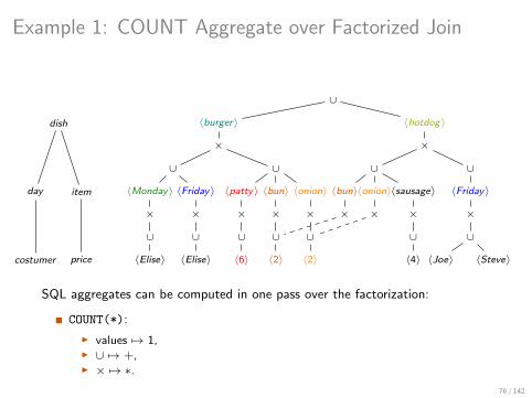
Example 1: COUNT Aggregate over Factorized Join
∪
〈burger〉 〈hotdog〉
× ×
∪
〈sausage〉〈bun〉〈onion〉
×× ×
∪
〈4〉
∪
〈Friday〉
×
∪
〈Joe〉 〈Steve〉
∪
〈patty〉 〈bun〉 〈onion〉
× × ×
∪ ∪ ∪
〈6〉 〈2〉 〈2〉
∪
〈Friday〉
×
∪
〈Elise〉
〈Monday〉
×
∪
〈Elise〉
dish
day item
costumer price
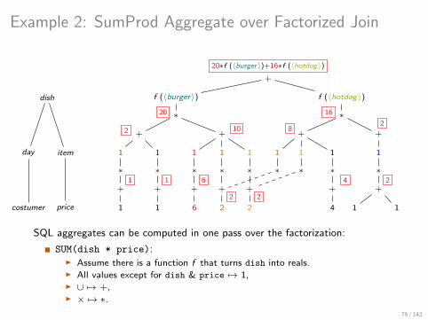
SQL aggregates can be computed in one pass over the factorization:
COUNT(*):
I values 7→ 1,I ∪ 7→ +,I × 7→ ∗.
76 / 142

Example 1: COUNT Aggregate over Factorized Join
+
1 1
∗ ∗
+
11 1
∗∗ ∗
+
1
+
1
∗
+
1 1
+
1 1 1
∗ ∗ ∗
+ + +
1 1 1
+
1
∗
+
1
1
∗
+
1
dish
day item
costumer price
12
66
2 3
1 1 1
1 1
3 2
1 2
SQL aggregates can be computed in one pass over the factorization:
COUNT(*):
I values 7→ 1,I ∪ 7→ +,I × 7→ ∗.
77 / 142
Example 2: SumProd Aggregate over Factorized Join
∪
〈burger〉 〈hotdog〉
× ×
∪
〈sausage〉〈bun〉〈onion〉
×× ×
∪
〈4〉
∪
〈Friday〉
×
∪
〈Joe〉 〈Steve〉
∪
〈patty〉 〈bun〉 〈onion〉
× × ×
∪ ∪ ∪
〈6〉 〈2〉 〈2〉
∪
〈Friday〉
×
∪
〈Elise〉
〈Monday〉
×
∪
〈Elise〉
dish
day item
costumer price
SQL aggregates can be computed in one pass over the factorization:
SUM(dish * price):I Assume there is a function f that turns dish into reals.I All values except for dish & price 7→ 1,I ∪ 7→ +,I × 7→ ∗.
78 / 142
Example 2: SumProd Aggregate over Factorized Join
+
f (〈burger〉) f (〈hotdog〉)
∗ ∗
+
11 1
∗∗ ∗
+
4
+
1
∗
+
1 1
+
1 1 1
∗ ∗ ∗
+ + +
6 2 2
+
1
∗
+
1
1
∗
+
1
dish
day item
costumer price
20∗f (〈burger〉)+16∗f (〈hotdog〉)
1620
2 10
1 1 6
2 2
82
4 2
SQL aggregates can be computed in one pass over the factorization:
SUM(dish * price):I Assume there is a function f that turns dish into reals.I All values except for dish & price 7→ 1,I ∪ 7→ +,I × 7→ ∗.
79 / 142
Example: Factorized Aggregate Computation
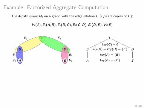
The 4-path query Q4 on a graph with the edge relation E (Ei ’s are copies of E):
V1(A),E1(A,B),E2(B,C),E3(C ,D),E4(D,E),V2(E)
C
B D
A EV1 V2
E1 E4
E2 E3 C
B D
A E
key(A) = B
key(E) = D
key(B) = key(D) = Ckey(C) = ∅
Recall sizes for factorized results of path queries
ρ∗(Q4) = 3⇒ listing representation has size O(|E |3).
s(Q4) = 2⇒ factorization without caching has size O(|E |2).
fhtw(Q4) = 1⇒ factorization with caching has size O(|E |).
For the n-path query Qn, s(Qn) = log2 n and fhtw(Qn) = 1.
80 / 142

Example: Factorized Aggregate Computation
We would like to compute COUNT(Q4):
in (pseudo)linear time
using optimized queries that are derived from the variable order of Q4
without materializing the factorized result of the path query
Convention:
View the relations as functions mapping tuples to numbers.
The functions for input relations map their tuples to 1.
81 / 142

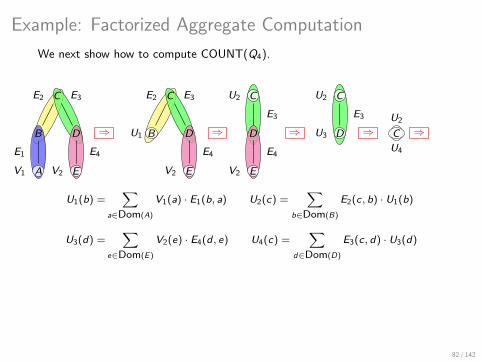
Example: Factorized Aggregate Computation
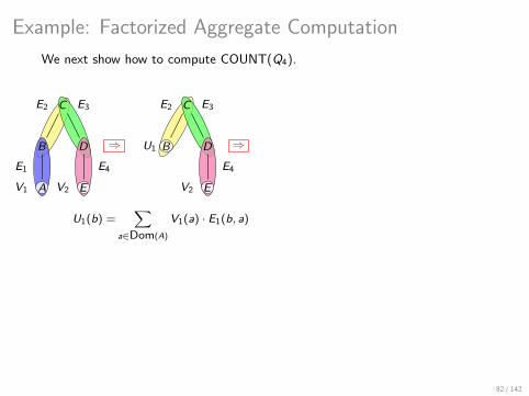
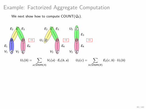
We next show how to compute COUNT(Q4).
V1 V2
E1 E4
E2 E3C
B D
A E
⇒
C
B D
E
U1
E2
V2
E3
E4
⇒
C
D
E
U2
E3
V2
E4
⇒
C
D
U2
E3
U3 ⇒ C
U2
U4
⇒U5
U1(b) =∑
a∈Dom(A)
V1(a) · E1(b, a) U2(c) =∑
b∈Dom(B)
E2(c, b) · U1(b)
U3(d) =∑
e∈Dom(E)
V2(e) · E4(d , e) U4(c) =∑
d∈Dom(D)
E3(c, d) · U3(d)
U5 =∑
c∈Dom(C)
U2(c) · U4(c)
82 / 142
Example: Factorized Aggregate Computation
We next show how to compute COUNT(Q4).
V1 V2
E1 E4
E2 E3C
B D
A E
⇒
C
B D
E
U1
E2
V2
E3
E4
⇒
C
D
E
U2
E3
V2
E4
⇒
C
D
U2
E3
U3 ⇒ C
U2
U4
⇒U5
U1(b) =∑
a∈Dom(A)
V1(a) · E1(b, a)
U2(c) =∑
b∈Dom(B)
E2(c, b) · U1(b)
U3(d) =∑
e∈Dom(E)
V2(e) · E4(d , e) U4(c) =∑
d∈Dom(D)
E3(c, d) · U3(d)
U5 =∑
c∈Dom(C)
U2(c) · U4(c)
82 / 142
Example: Factorized Aggregate Computation
We next show how to compute COUNT(Q4).
V1 V2
E1 E4
E2 E3C
B D
A E
⇒
C
B D
E
U1
E2
V2
E3
E4
⇒
C
D
E
U2
E3
V2
E4
⇒
C
D
U2
E3
U3 ⇒ C
U2
U4
⇒U5
U1(b) =∑
a∈Dom(A)
V1(a) · E1(b, a) U2(c) =∑
b∈Dom(B)
E2(c, b) · U1(b)
U3(d) =∑
e∈Dom(E)
V2(e) · E4(d , e) U4(c) =∑
d∈Dom(D)
E3(c, d) · U3(d)
U5 =∑
c∈Dom(C)
U2(c) · U4(c)
82 / 142

Example: Factorized Aggregate Computation
We next show how to compute COUNT(Q4).
V1 V2
E1 E4
E2 E3C
B D
A E
⇒
C
B D
E
U1
E2
V2
E3
E4
⇒
C
D
E
U2
E3
V2
E4
⇒
C
D
U2
E3
U3 ⇒
C
U2
U4
⇒U5
U1(b) =∑
a∈Dom(A)
V1(a) · E1(b, a) U2(c) =∑
b∈Dom(B)
E2(c, b) · U1(b)
U3(d) =∑
e∈Dom(E)
V2(e) · E4(d , e)
U4(c) =∑
d∈Dom(D)
E3(c, d) · U3(d)
U5 =∑
c∈Dom(C)
U2(c) · U4(c)
82 / 142
Example: Factorized Aggregate Computation
We next show how to compute COUNT(Q4).
V1 V2
E1 E4
E2 E3C
B D
A E
⇒
C
B D
E
U1
E2
V2
E3
E4
⇒
C
D
E
U2
E3
V2
E4
⇒
C
D
U2
E3
U3 ⇒ C
U2
U4
⇒
U5
U1(b) =∑
a∈Dom(A)
V1(a) · E1(b, a) U2(c) =∑
b∈Dom(B)
E2(c, b) · U1(b)
U3(d) =∑
e∈Dom(E)
V2(e) · E4(d , e) U4(c) =∑
d∈Dom(D)
E3(c, d) · U3(d)
U5 =∑
c∈Dom(C)
U2(c) · U4(c)
82 / 142

Example: Factorized Aggregate Computation
We next show how to compute COUNT(Q4).
V1 V2
E1 E4
E2 E3C
B D
A E
⇒
C
B D
E
U1
E2
V2
E3
E4
⇒
C
D
E
U2
E3
V2
E4
⇒
C
D
U2
E3
U3 ⇒ C
U2
U4
⇒U5
U1(b) =∑
a∈Dom(A)
V1(a) · E1(b, a) U2(c) =∑
b∈Dom(B)
E2(c, b) · U1(b)
U3(d) =∑
e∈Dom(E)
V2(e) · E4(d , e) U4(c) =∑
d∈Dom(D)
E3(c, d) · U3(d)
U5 =∑
c∈Dom(C)
U2(c) · U4(c)
82 / 142
Functional Aggregate Queries
83 / 142
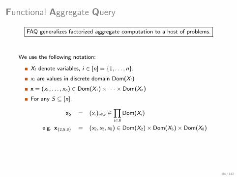
Functional Aggregate Query
FAQ generalizes factorized aggregate computation to a host of problems.
We use the following notation:
Xi denote variables, i ∈ [n] = 1, . . . , n,
xi are values in discrete domain Dom(Xi )
x = (x1, . . . , xn) ∈ Dom(X1)× · · · × Dom(Xn)
For any S ⊆ [n],
xS = (xi )i∈S ∈∏i∈S
Dom(Xi )
e.g. x2,5,8 = (x2, x5, x8) ∈ Dom(X2)× Dom(X5)× Dom(X8)
84 / 142
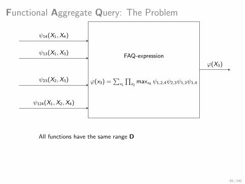
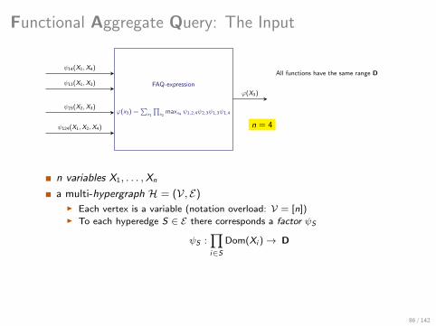
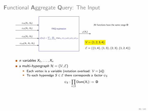
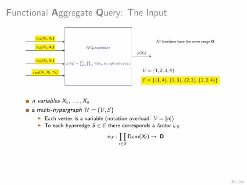
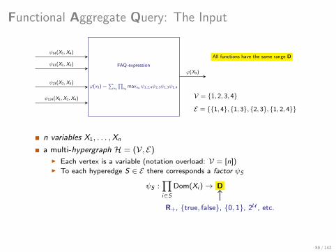
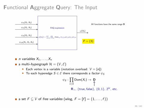
Functional Aggregate Query: The Problem
FAQ-expression
ϕ(x3) =∑
x1
∏x2
maxx4 ψ1,2,4ψ2,3ψ1,3ψ1,4
ϕ(X3)
ψ124(X1,X2,X4)
ψ23(X2,X3)
ψ13(X1,X3)
ψ14(X1,X4)
All functions have the same range D
85 / 142
Functional Aggregate Query: The Input
FAQ-expression
ϕ(x3) =∑
x1
∏x2
maxx4 ψ1,2,4ψ2,3ψ1,3ψ1,4
ϕ(X3)
ψ124(X1,X2,X4)
ψ23(X2,X3)
ψ13(X1,X3)
ψ14(X1,X4)All functions have the same range D
n = 4
V = 1, 2, 3, 4
E = 1, 4, 1, 3, 2, 3, 1, 2, 4
V = 1, 2, 3, 4
E = 1, 4, 1, 3, 2, 3, 1, 2, 4
F = 3
n variables X1, . . . ,Xn
a multi-hypergraph H = (V, E)I Each vertex is a variable (notation overload: V = [n])I To each hyperedge S ∈ E there corresponds a factor ψS
ψS :∏i∈S
Dom(Xi )→ D
a set F ⊆ V of free variables (wlog, F = [f ] = 1, . . . , f )
86 / 142
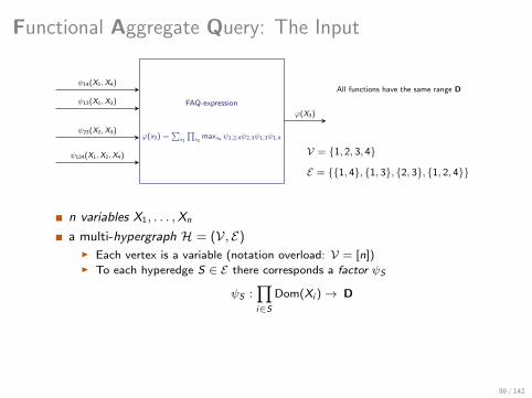
Functional Aggregate Query: The Input
FAQ-expression
ϕ(x3) =∑
x1
∏x2
maxx4 ψ1,2,4ψ2,3ψ1,3ψ1,4
ϕ(X3)
ψ124(X1,X2,X4)
ψ23(X2,X3)
ψ13(X1,X3)
ψ14(X1,X4)All functions have the same range D
n = 4
V = 1, 2, 3, 4
E = 1, 4, 1, 3, 2, 3, 1, 2, 4
V = 1, 2, 3, 4
E = 1, 4, 1, 3, 2, 3, 1, 2, 4
F = 3
n variables X1, . . . ,Xn
a multi-hypergraph H = (V, E)I Each vertex is a variable (notation overload: V = [n])I To each hyperedge S ∈ E there corresponds a factor ψS
ψS :∏i∈S
Dom(Xi )→ D
R+, true, false, 0, 1, 2U , etc.
a set F ⊆ V of free variables (wlog, F = [f ] = 1, . . . , f )
86 / 142
Functional Aggregate Query: The Input
FAQ-expression
ϕ(x3) =∑
x1
∏x2
maxx4 ψ1,2,4ψ2,3ψ1,3ψ1,4
ϕ(X3)
ψ124(X1,X2,X4)
ψ23(X2,X3)
ψ13(X1,X3)
ψ14(X1,X4)All functions have the same range D
n = 4V = 1, 2, 3, 4
E = 1, 4, 1, 3, 2, 3, 1, 2, 4
V = 1, 2, 3, 4
E = 1, 4, 1, 3, 2, 3, 1, 2, 4
F = 3
n variables X1, . . . ,Xn
a multi-hypergraph H = (V, E)I Each vertex is a variable (notation overload: V = [n])I To each hyperedge S ∈ E there corresponds a factor ψS
ψS :∏i∈S
Dom(Xi )→ D
R+, true, false, 0, 1, 2U , etc.
a set F ⊆ V of free variables (wlog, F = [f ] = 1, . . . , f )
86 / 142

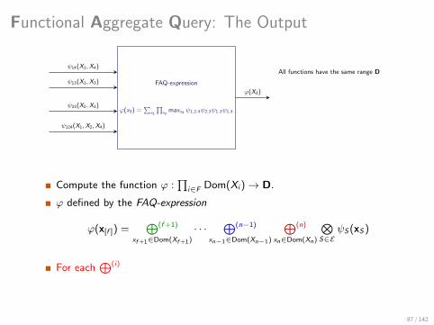
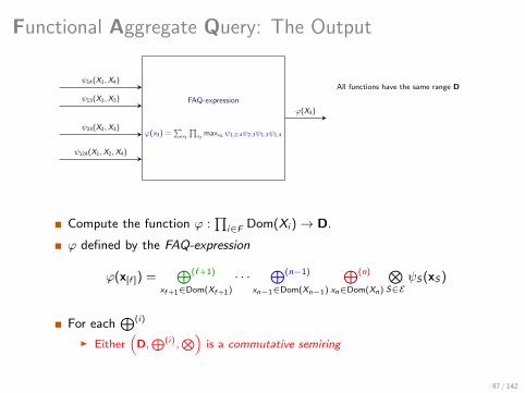
Functional Aggregate Query: The Output
FAQ-expression
ϕ(x3) =∑
x1
∏x2
maxx4 ψ1,2,4ψ2,3ψ1,3ψ1,4
ϕ(X3)
ψ124(X1,X2,X4)
ψ23(X2,X3)
ψ13(X1,X3)
ψ14(X1,X4)All functions have the same range D
Compute the function ϕ :∏
i∈F Dom(Xi )→ D.
ϕ defined by the FAQ-expression
ϕ(x[f ]) =⊕(f +1)
xf +1∈Dom(Xf +1)
· · ·⊕(n−1)
xn−1∈Dom(Xn−1)
⊕(n)
xn∈Dom(Xn)
⊗S∈E
ψS(xS)
For each⊕(i)
I Either(
D,⊕(i),
⊗)is a commutative semiring
I Or⊕(i) =
⊗
87 / 142

Functional Aggregate Query: The Output
FAQ-expression
ϕ(x3) =∑
x1
∏x2
maxx4 ψ1,2,4ψ2,3ψ1,3ψ1,4
ϕ(X3)
ψ124(X1,X2,X4)
ψ23(X2,X3)
ψ13(X1,X3)
ψ14(X1,X4)All functions have the same range D
Compute the function ϕ :∏
i∈F Dom(Xi )→ D.
ϕ defined by the FAQ-expression
ϕ(x[f ]) =⊕(f +1)
xf +1∈Dom(Xf +1)
· · ·⊕(n−1)
xn−1∈Dom(Xn−1)
⊕(n)
xn∈Dom(Xn)
⊗S∈E
ψS(xS)
For each⊕(i)
I Either(
D,⊕(i),
⊗)is a commutative semiring
I Or⊕(i) =
⊗87 / 142

Semirings
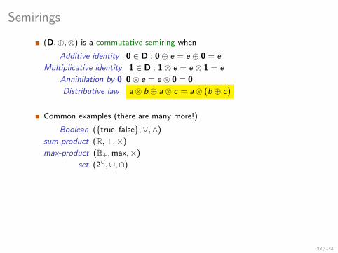
(D,⊕,⊗) is a commutative semiring when
Additive identity 0 ∈ D : 0⊕ e = e ⊕ 0 = e
Multiplicative identity 1 ∈ D : 1⊗ e = e ⊗ 1 = e
Annihilation by 0 0⊗ e = e ⊗ 0 = 0
Distributive law a⊗ b ⊕ a⊗ c = a⊗ (b ⊕ c)
Common examples (there are many more!)
Boolean (true, false,∨,∧)
sum-product (R,+,×)
max-product (R+,max,×)
set (2U ,∪,∩)
88 / 142
Semirings
(D,⊕,⊗) is a commutative semiring when
Additive identity 0 ∈ D : 0⊕ e = e ⊕ 0 = e
Multiplicative identity 1 ∈ D : 1⊗ e = e ⊗ 1 = e
Annihilation by 0 0⊗ e = e ⊗ 0 = 0
Distributive law a⊗ b ⊕ a⊗ c = a⊗ (b ⊕ c)
Common examples (there are many more!)
Boolean (true, false,∨,∧)
sum-product (R,+,×)
max-product (R+,max,×)
set (2U ,∪,∩)
88 / 142

SumProduct ⊂ FAQ
Problem (SumProduct)
Given a commutative semiring (D,⊕,⊗), compute the function
ϕ(x1, . . . , xf ) =⊕xf +1
⊕xf +2
· · ·⊕xn
⊗S∈E
ψS(xS)
SumProductI Rina Dechter (Artificial Intelligence 1999 and earlier)
≡ Marginalize a Product FunctionI Aji and McEliece (IEEE Trans. Inform. Theory 2000)
89 / 142
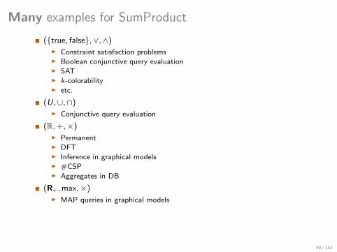
Many examples for SumProduct
(true, false,∨,∧)I Constraint satisfaction problemsI Boolean conjunctive query evaluationI SATI k-colorabilityI etc.
(U,∪,∩)I Conjunctive query evaluation
(R,+,×)I PermanentI DFTI Inference in graphical modelsI #CSPI Aggregates in DB
(R+,max,×)I MAP queries in graphical models
90 / 142
Part 1. Joins
Part 2. Aggregates
Part 3. Optimization
Part 4. Open Problems
91 / 142
Outline
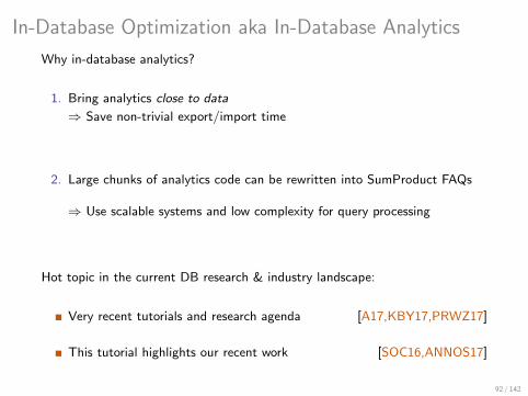
In-Database Optimization aka In-Database Analytics
Why in-database analytics?
1. Bring analytics close to data
⇒ Save non-trivial export/import time
2. Large chunks of analytics code can be rewritten into SumProduct FAQs
⇒ Use scalable systems and low complexity for query processing
Hot topic in the current DB research & industry landscape:
Very recent tutorials and research agenda [A17,KBY17,PRWZ17]
This tutorial highlights our recent work [SOC16,ANNOS17]
92 / 142
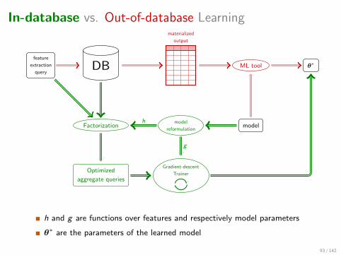
In-database vs. Out-of-database Learning
feature
extraction
queryDB
materialized
output
ML tool θ∗
modelmodel
reformulationFactorization
Optimized
aggregate queries
Gradient-descent
Trainer
h
g
h and g are functions over features and respectively model parameters
θ∗ are the parameters of the learned model
93 / 142
Our Approach to In-Database Analytics
Unified in-database analytics solution for a host of optimization problems.
Used by retail-planning and forecasting applications
Typical databases have weekly sales, promotions, and products
Training dataset = Result of a feature extraction query over the database
Task = Train parameterized model to predict, e.g., additional demand
generated for a product due to promotion
Training algorithm = First-order optimization algorithm, e.g., batch or
stochastic gradient descent, whose convergence rates are dimension-free
Commercial database management system
One platform for OLAP and OLTP, descriptive and predictive analytics
Datalog++ as programming language for applications
94 / 142
Plan for Tutorial Part 3
We will first introduce the main technical ideas via an example
I Train a linear regression model using batch gradient descent
I Express gradient computation as database queries
I Re-parameterize the model under functional dependencies
We will then discuss a generalization
I Polynomial regression, factorization machines, classification
We will conclude with complexity analysis of in-database analytics
I Model training faster than computing the input to external ML library!
95 / 142
Typical Retail Example
96 / 142
Typical Retail Example
Database I = (R1,R2,R3,R4,R5)
Feature selection query Q:
Q(sku, store, color, city, country, unitsSold)←
R1(sku, store, day, unitsSold),R2(sku, color),
R3(day, quarter),R4(store, city),R5(city, country).
Free variablesI Categorical (qualitative): F = sku, store, color, city, country.I Continuous (quantitative): unitsSold.
Bounded variablesI Categorical (qualitative): B = day, quarter
We learn the ridge linear regression model 〈θ, x〉 =∑
f∈F 〈θf , xf 〉 over
D = Q(I ) with feature vector x and response yunitsSold .
The parameters θ are obtained by minimizing the square loss function:
J(θ) =1
2|D|∑
(x,y)∈D
(〈θ, x〉 − yunitsSold)2 + ‖θ‖22
97 / 142
Recap: One-hot encoding of categorical variables
Continuous variables are mapped to scalars
I yunitsSold ∈ R.
Categorical variables are mapped to indicator vectors
I Say variable country has categories vietnam and england.
I The variable country is then mapped to an indicator vector
xcountry = [xvietnam, xengland]> ∈ (0, 12)>.
I xcountry = [0, 1]> for a tuple with country = ‘‘england’’
One-hot encoding leads to very wide training datasets and many 0-values.
98 / 142

Recap: Role of the Least Square Loss Function
Goal: Describe a linear relationship fun(x) = θ1x + θ0 between variables x and
y = fun(x), so we can estimate new y values given new x values.
We are given n (black) data points (xi , yi )i∈[n]
We would like to find a (red) regression line fun(x) such that the (green)
error∑
i∈[n](fun(xi )− yi )2 is minimized
The role of the `2-regularization ‖θ‖22 = θ2
0 + θ21 is to avoid
over/under-fitting. It gives preference to functions fun with smaller norms.
99 / 142

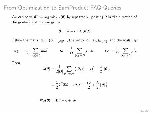
From Optimization to SumProduct FAQ Queries
We can solve θ∗ := arg minθ J(θ) by repeatedly updating θ in the direction of
the gradient until convergence:
θ := θ − α ·∇J(θ).
Define the matrix Σ = (σij)i,j∈[|F |], the vector c = (ci )i∈[|F |], and the scalar sY :
σij =1
|D|∑
(x,y)∈D
xix>j ci =
1
|D|∑
(x,y)∈D
y · xi sY =1
|D|∑
(x,y)∈D
y 2.
Then,
J(θ) =1
2|D|∑
(x,y)∈D
(〈θ, x〉 − y)2 +λ
2‖θ‖2
2
=1
2θ>Σθ − 〈θ, c〉+
sY2
+λ
2‖θ‖2
2
∇J(θ) = Σθ − c + λθ
100 / 142
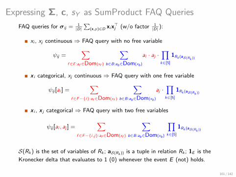
Expressing Σ, c, sY as SumProduct FAQ Queries
FAQ queries for σij = 1|D|∑
(x,y)∈D xix>j (w/o factor 1
|D| ):
xi , xj continuous ⇒ FAQ query with no free variable
ψij =∑
f∈F :af ∈Dom(xf )
∑b∈B:ab∈Dom(xb)
ai · aj ·∏k∈[5]
1Rk (aS(Rk ))
x i categorical, xj continuous ⇒ FAQ query with one free variable
ψij [ai ] =∑
f∈F−i:af ∈Dom(xf )
∑b∈B:ab∈Dom(xb)
aj ·∏k∈[5]
1Rk (aS(Rk ))
x i , x j categorical ⇒ FAQ query with two free variables
ψij [ai , aj ] =∑
f∈F−i,j:af ∈Dom(xf )
∑b∈B:ab∈Dom(xb)
∏k∈[5]
1Rk (aS(Rk ))
S(Rk) is the set of variables of Rk ; aS(Rk )) is a tuple in relation Rk ; 1E is the
Kronecker delta that evaluates to 1 (0) whenever the event E (not) holds.
101 / 142

Expressing Σ, c, sY as SQL Queries
SQL queries for σij = 1|D|∑
(x,y)∈D xix>j (w/o factor 1
|D| ):
xi , xj continuous ⇒ SQL query with no group-by attribute
SELECT SUM(xi*xj) FROM D;
x i categorical, xj continuous ⇒ SQL query with one group-by attribute
SELECT xi , SUM(xj) FROM D GROUP BY xi ;
x i , x j categorical ⇒ SQL query with two free variables
SELECT xi , xj , SUM(1) FROM D GROUP BY xi , xj ;
Σ, c, sY are all aggregates that can be computed inside the database!
We avoid one-hot/sparse encoding of the input data.
102 / 142
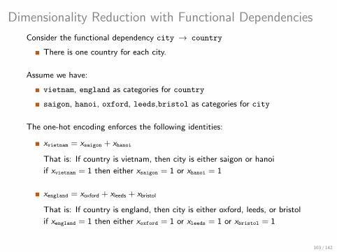
Dimensionality Reduction with Functional Dependencies
Consider the functional dependency city → country
There is one country for each city.
Assume we have:
vietnam, england as categories for country
saigon, hanoi, oxford, leeds,bristol as categories for city
The one-hot encoding enforces the following identities:
xvietnam = xsaigon + xhanoi
That is: If country is vietnam, then city is either saigon or hanoi
if xvietnam = 1 then either xsaigon = 1 or xhanoi = 1
xengland = xoxford + xleeds + xbristol
That is: If country is england, then city is either oxford, leeds, or bristol
if xengland = 1 then either xoxford = 1 or xleeds = 1 or xbristol = 1
103 / 142
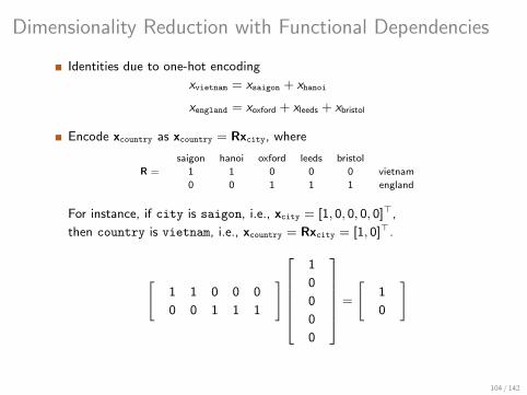
Dimensionality Reduction with Functional Dependencies
Identities due to one-hot encoding
xvietnam = xsaigon + xhanoi
xengland = xoxford + xleeds + xbristol
Encode xcountry as xcountry = Rxcity, where
R =
saigon hanoi oxford leeds bristol
1 1 0 0 0 vietnam
0 0 1 1 1 england
For instance, if city is saigon, i.e., xcity = [1, 0, 0, 0, 0]>,
then country is vietnam, i.e., xcountry = Rxcity = [1, 0]>.
[1 1 0 0 0
0 0 1 1 1
]1
0
0
0
0
=
[1
0
]
104 / 142
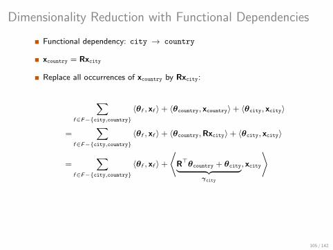
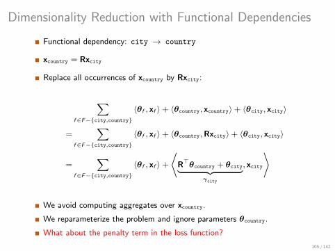
Dimensionality Reduction with Functional Dependencies
Functional dependency: city → country
xcountry = Rxcity
Replace all occurrences of xcountry by Rxcity:
∑f∈F−city,country
〈θf , xf 〉+ 〈θcountry, xcountry〉+ 〈θcity, xcity〉
=∑
f∈F−city,country
〈θf , xf 〉+ 〈θcountry,Rxcity〉+ 〈θcity, xcity〉
=∑
f∈F−city,country
〈θf , xf 〉+
⟨R>θcountry + θcity︸ ︷︷ ︸
γcity
, xcity
⟩
We avoid computing aggregates over xcountry.
We reparameterize the problem and ignore parameters θcountry.
What about the penalty term in the loss function?
105 / 142

Dimensionality Reduction with Functional Dependencies
Functional dependency: city → country
xcountry = Rxcity
γcity = R>θcountry + θcity
Rewrite the penalty term
‖θ‖22 =
∑j 6=city
‖θj‖22 +
∥∥∥γcity − R>θcountry
∥∥∥2
2+ ‖θcountry‖2
2
”Optimize out” θcountry by expressing it in terms of γcity:
θcountry = (Icountry + RR>)−1Rγcity = R(Icity + R>R)−1γcity
Icountry is the order-Ncountry identity matrix and similarly for Icity.
The penalty term becomes
‖θ‖22 =
∑j 6=city
‖θj‖22 +
⟨(Icity + R>R)−1γcity,γcity
⟩
106 / 142

The General Picture
107 / 142
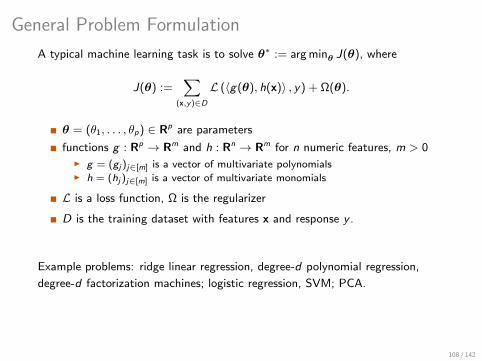
General Problem Formulation
A typical machine learning task is to solve θ∗ := arg minθ J(θ), where
J(θ) :=∑
(x,y)∈D
L (〈g(θ), h(x)〉 , y) + Ω(θ).
θ = (θ1, . . . , θp) ∈ Rp are parameters
functions g : Rp → Rm and h : Rn → Rm for n numeric features, m > 0I g = (gj )j∈[m] is a vector of multivariate polynomialsI h = (hj )j∈[m] is a vector of multivariate monomials
L is a loss function, Ω is the regularizer
D is the training dataset with features x and response y .
Example problems: ridge linear regression, degree-d polynomial regression,
degree-d factorization machines; logistic regression, SVM; PCA.
108 / 142
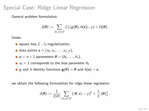
Special Case: Ridge Linear Regression
General problem formulation:
J(θ) :=∑
(x,y)∈D
L (〈g(θ), h(x)〉 , y) + Ω(θ).
Under
square loss L , `2-regularization,
data points x = (x0, x1, . . . , xn, y),
p = n + 1 parameters θ = (θ0, . . . , θn),
x0 = 1 corresponds to the bias parameter θ0
g and h identity functions g(θ) = θ and h(x) = x,
we obtain the following formulation for ridge linear regression:
J(θ) :=1
2|D|∑
(x,y)∈D
(〈θ, x〉 − y)2 +λ
2‖θ‖2
2 .
109 / 142
Special Case: Degree-d Polynomial Regression
General problem formulation:
J(θ) :=∑
(x,y)∈D
L (〈g(θ), h(x)〉 , y) + Ω(θ).
Under
square loss L , `2-regularization,
data points x = (x0, x1, . . . , xn, y),
p = m = 1 + n + n2 + · · ·+ nd parameters θ = (θa), where
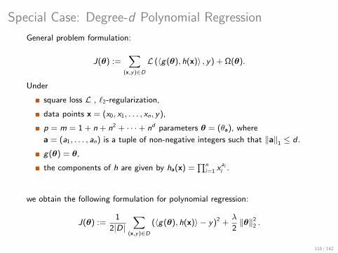
a = (a1, . . . , an) is a tuple of non-negative integers such that ‖a‖1 ≤ d .
g(θ) = θ,
the components of h are given by ha(x) =∏n
i=1 xaii .
we obtain the following formulation for polynomial regression:
J(θ) :=1
2|D|∑
(x,y)∈D
(〈g(θ), h(x)〉 − y)2 +λ
2‖θ‖2
2 .
110 / 142

Special Case: Factorization Machines
Under
square loss L , `2-regularization,
data points x = (x0, x1, . . . , xn, y),
p = m = 1 + n + r · n parameters and m = 1 + n +(n2
)features
we obtain the following formulation for degree-2 rank-r factorization machines:
J(θ) :=1
2|D|∑
(x,y)∈D
n∑
i=0
θixi +∑
i,j∈(
[n]2
)`∈[r ]
θ(`)i θ
(`)j xixj − y
2
+λ
2‖θ‖2
2 .
where
hS (x) =∏i∈S
xi , for S ⊆ [n], |S | ≤ 2
gS (θ) =
θ0 when |S | = 0
θi when S = i∑r`=1 θ
(`)i θ
(`)j when S = i , j.
111 / 142
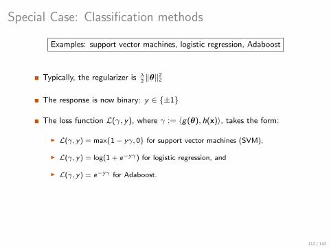
Special Case: Classification methods
Examples: support vector machines, logistic regression, Adaboost
Typically, the regularizer is λ2‖θ‖2
2
The response is now binary: y ∈ ±1
The loss function L(γ, y), where γ := 〈g(θ), h(x)〉, takes the form:
I L(γ, y) = max1− yγ, 0 for support vector machines (SVM),
I L(γ, y) = log(1 + e−yγ) for logistic regression, and
I L(γ, y) = e−yγ for Adaboost.
112 / 142
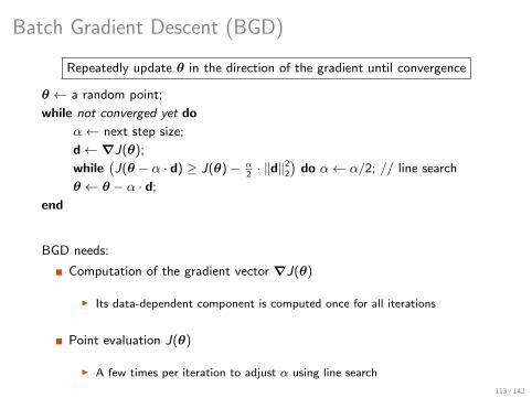
Batch Gradient Descent (BGD)
Repeatedly update θ in the direction of the gradient until convergence
θ ← a random point;
while not converged yet do
α← next step size;
d←∇J(θ);
while(J(θ − α · d) ≥ J(θ)− α
2· ‖d‖2
2
)do α← α/2; // line search
θ ← θ − α · d;
end
BGD needs:
Computation of the gradient vector ∇J(θ)
I Its data-dependent component is computed once for all iterations
Point evaluation J(θ)
I A few times per iteration to adjust α using line search
113 / 142

Compute Parameters θ using BGD
Immediate extension of the linear regression case discussed before.
Define the matrix Σ = (σij)i,j∈[m], the vector c = (ci )i∈[m], and the scalar sY by
Σ =1
|D|∑
(x,y)∈D
h(x)h(x)>
c =1
|D|∑
(x,y)∈D
y · h(x)
sY =1
|D|∑
(x,y)∈D
y 2.
Under square loss L and `2-regularization:
J(θ) =1
2g(θ)>Σg(θ)− 〈g(θ), c〉+
sY2
+λ
2‖θ‖2
2
∇J(θ) =∂g(θ)>
∂θΣg(θ)− ∂g(θ)>
∂θc + λθ
114 / 142

Summing Up
Insight #1:
Σ, c, sY are queries that can be computed inside the database!
I They can take much less time than computing the feature extraction query
Insight #2:
The training dataset has repeating data blocks as it satisfies the join
dependencies given by the feature extraction query.
I A factorized training dataset avoids this redundancy.
Insight #3:
The training dataset has many functional dependencies in practice.
I First learn a smaller, reparameterized model whose features functionally
determine the left-out features, then map it back to the original model with
both functionally determining and determined parameters
115 / 142
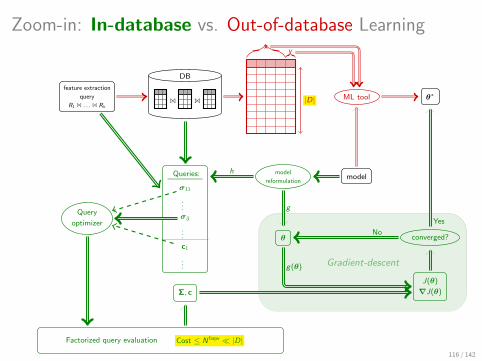
Zoom-in: In-database vs. Out-of-database Learning
feature extraction
query
R1 1 . . . 1 Rk
DB
1 1
xy
|D| ML tool θ∗
modelmodel
reformulationQueries:
σ11
...σij
...
c1
...
Query
optimizer
Factorized query evaluation Cost ≤ N faqw |D|
Σ, c
θ
J(θ)
∇J(θ)
converged?
Gradient-descent
h
g
g(θ)
No
Yes
116 / 142

Complexity Analysis
117 / 142
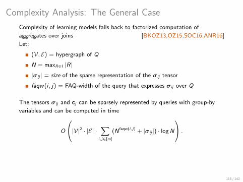
Complexity Analysis: The General Case
Complexity of learning models falls back to factorized computation of
aggregates over joins [BKOZ13,OZ15,SOC16,ANR16]
Let:
(V, E) = hypergraph of Q
N = maxR∈I |R|
|σij | = size of the sparse representation of the σij tensor
faqw(i , j) = FAQ-width of the query that expresses σij over Q
The tensors σij and cj can be sparsely represented by queries with group-by
variables and can be computed in time
O
|V|2 · |E| · ∑i,j∈[m]
(N faqw(i,j) + |σij |) · logN
.
118 / 142
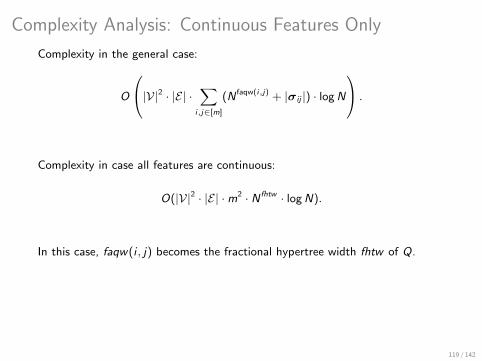
Complexity Analysis: Continuous Features Only
Complexity in the general case:
O
|V|2 · |E| · ∑i,j∈[m]
(N faqw(i,j) + |σij |) · logN
.
Complexity in case all features are continuous:
O(|V|2 · |E| ·m2 · N fhtw · logN).
In this case, faqw(i , j) becomes the fractional hypertree width fhtw of Q.
119 / 142
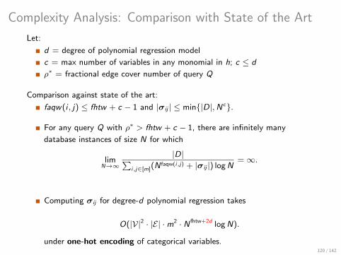
Complexity Analysis: Comparison with State of the Art
Let:
d = degree of polynomial regression model
c = max number of variables in any monomial in h; c ≤ d
ρ∗ = fractional edge cover number of query Q
Comparison against state of the art:
faqw(i , j) ≤ fhtw + c − 1 and |σij | ≤ min|D|,Nc.
For any query Q with ρ∗ > fhtw + c − 1, there are infinitely many
database instances of size N for which
limN→∞
|D|∑i,j∈[m](N
faqw(i,j) + |σij |) logN=∞.
Computing σij for degree-d polynomial regression takes
O(|V|2 · |E| ·m2 · N fhtw+2d logN).
under one-hot encoding of categorical variables.120 / 142
Part 1. Joins
Part 2. Aggregates
Part 3. Optimization
Part 4. Open Problems
121 / 142
Outline

Adaptive Join Processing
122 / 142
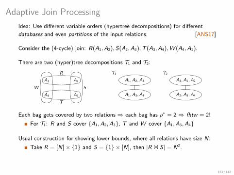
Adaptive Join Processing
Idea: Use different variable orders (hypertree decompositions) for different
databases and even partitions of the input relations. [ANS17]
Consider the (4-cycle) join: R(A1,A2),S(A2,A3),T (A3,A4),W (A4,A1).
There are two (hyper)tree decompositions T1 and T2:
R
T
W S
A1 A2
A3A4
T1
A1,A2,A3
A1,A3,A4
T2
A4,A1,A2
A2,A3,A4
Each bag gets covered by two relations ⇒ each bag has ρ∗ = 2 ⇒ fhtw = 2!
For T1: R and S cover A1,A2,A3, T and W cover A1,A3,A4
Usual construction for showing lower bounds, where all relations have size N:
Take R = [N]× 1 and S = 1 × [N], then |R 1 S | = N2.
These R and S do not yield N2 for T2!: R and W cover A4,A1,A2 with
|R 1 W | = N, while S and T cover A2,A3,A4 with |S 1 T | = N.
123 / 142

Adaptive Join Processing
Idea: Use different variable orders (hypertree decompositions) for different
databases and even partitions of the input relations. [ANS17]
Consider the (4-cycle) join: R(A1,A2),S(A2,A3),T (A3,A4),W (A4,A1).
There are two (hyper)tree decompositions T1 and T2:
R
T
W S
A1 A2
A3A4
T1
A1,A2,A3
A1,A3,A4
T2
A4,A1,A2
A2,A3,A4
Each bag gets covered by two relations ⇒ each bag has ρ∗ = 2 ⇒ fhtw = 2!
For T1: R and S cover A1,A2,A3, T and W cover A1,A3,A4
Usual construction for showing lower bounds, where all relations have size N:
Take R = [N]× 1 and S = 1 × [N], then |R 1 S | = N2.
These R and S do not yield N2 for T2!: R and W cover A4,A1,A2 with
|R 1 W | = N, while S and T cover A2,A3,A4 with |S 1 T | = N.123 / 142
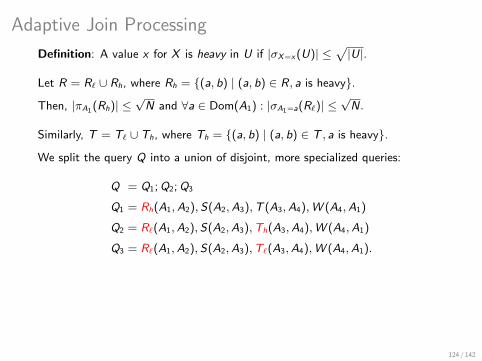
Adaptive Join Processing
Definition: A value x for X is heavy in U if |σX=x(U)| ≤√|U|.
Let R = R` ∪ Rh, where Rh = (a, b) | (a, b) ∈ R, a is heavy.
Then, |πA1 (Rh)| ≤√N and ∀a ∈ Dom(A1) : |σA1=a(R`)| ≤
√N.
Similarly, T = T` ∪ Th, where Th = (a, b) | (a, b) ∈ T , a is heavy.
We split the query Q into a union of disjoint, more specialized queries:
Q = Q1;Q2;Q3
Q1 = Rh(A1,A2),S(A2,A3),T (A3,A4),W (A4,A1)
Q2 = R`(A1,A2), S(A2,A3),Th(A3,A4),W (A4,A1)
Q3 = R`(A1,A2), S(A2,A3),T`(A3,A4),W (A4,A1).
Each of Q1,Q2,Q3 has fhtw = 3/2, hence Q has fhtw = 3/2.
124 / 142
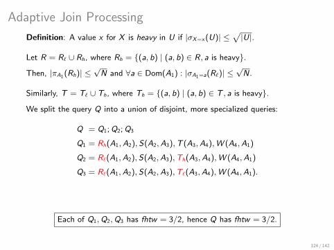
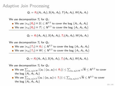
Adaptive Join Processing
Q1 = Rh(A1,A2),S(A2,A3),T (A3,A4),W (A4,A1)
We use decomposition T1 for Q1:
We use |πA1 (Rh) 1 S | ≤ N3/2 to cover the bag A1,A2,A3We use |πA1 (Rh) 1 T | ≤ N3/2 to cover the bag A1,A3,A4
Q2 = R`(A1,A2), S(A2,A3),Th(A3,A4),W (A4,A1)
We use decomposition T1 for Q2:
We use |πA3 (Th) 1 R`| ≤ N3/2 to cover the bag A1,A2,A3We use |πA3 (Th) 1 W | ≤ N3/2 to cover the bag A1,A3,A4
Q3 = R`(A1,A2), S(A2,A3),T`(A3,A4),W (A4,A1).
We use decomposition T2 for Q3:
We use∑
(a1,a4)∈W |a2 | (a1, a2) ∈ R`| ≤∑
(a1,a4)∈W
√N ≤ N3/2 to cover
the bag A1,A2,A4We use
∑(a2,a3)∈S |a4 | (a3, a4) ∈ T`| ≤
∑(a2,a3)∈S
√N ≤ N3/2 to cover
the bag A2,A3,A4125 / 142

One-join-at-a-time vs All-joins-at-once
126 / 142
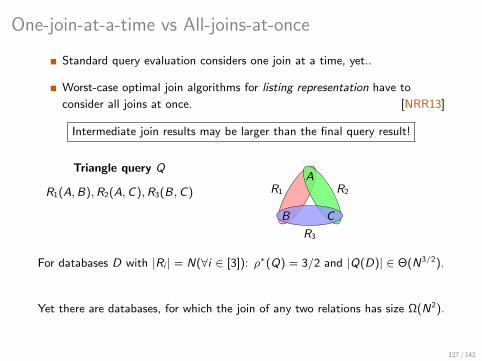
One-join-at-a-time vs All-joins-at-once
Standard query evaluation considers one join at a time, yet..
Worst-case optimal join algorithms for listing representation have to
consider all joins at once. [NRR13]
Intermediate join results may be larger than the final query result!
Triangle query Q
R1(A,B),R2(A,C),R3(B,C) R1 R2
R3
A
B C
For databases D with |Ri | = N(∀i ∈ [3]): ρ∗(Q) = 3/2 and |Q(D)| ∈ Θ(N3/2).
Yet there are databases, for which the join of any two relations has size Ω(N2).
127 / 142

Why traditional join-at-a-time plans are suboptimalQuery Q R1(A,B),R2(A,C),R3(B,C)
Database
R1 R2 R3 Q
A B
a0 b0
a0 . . .
a0 bm
a1 b0
. . . b0
am b0
A C
a0 c0
a0 . . .
a0 cm
a1 c0
. . . c0
am c0
B C
b0 c0
b0 . . .
b0 cm
b1 c0
. . . c0
bm c0
A B C
a0 b0 c0
a0 b0 . . .
a0 b0 cm
a0 b1 c0
a0 . . . c0
a0 bm c0
a1 b0 c0
a1 b0 c0
. . . b0 c0
Query plans
1
1 R1
R2 R3
1
1 R2
R1 R3
1
1 R3
R1 R2
. . .
128 / 142
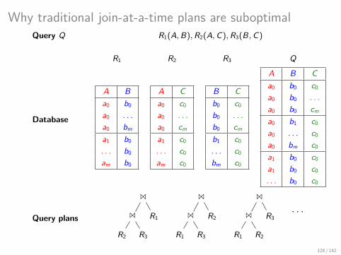

Why traditional join-at-a-time plans are suboptimalR1(A,B),R2(A,C),R3(B,C)
R1 R2 R3 Q
A B
a0 b0
a0 . . .
a0 bm
a1 b0
. . . b0
am b0
A C
a0 c0
a0 . . .
a0 cm
a1 c0
. . . c0
am c0
B C
b0 c0
b0 . . .
b0 cm
b1 c0
. . . c0
bm c0
A B C
a0 b0 c0
a0 b0 . . .
a0 b0 cm
a0 b1 c0
a0 . . . c0
a0 bm c0
a1 b0 c0
. . . b0 c0
a1 b0 c0
2m + 1 2m + 1 2m + 1 6m + 3
129 / 142
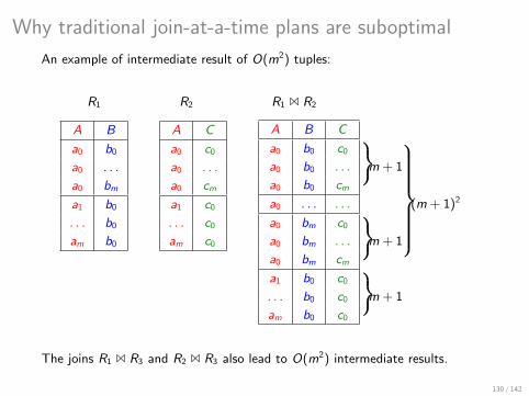
Why traditional join-at-a-time plans are suboptimal
An example of intermediate result of O(m2) tuples:
R1 R2 R1 1 R2
A B
a0 b0
a0 . . .
a0 bm
a1 b0
. . . b0
am b0
A C
a0 c0
a0 . . .
a0 cm
a1 c0
. . . c0
am c0
A B C
a0 b0 c0
︸︷︷︸
︸︷︷
︸
a0 b0 . . . m + 1
a0 b0 cm
a0 . . . . . . (m + 1)2
a0 bm c0
︸︷︷︸
a0 bm . . . m + 1
a0 bm cm
a1 b0 c0
︸︷︷︸
. . . b0 c0 m + 1
am b0 c0
The joins R1 1 R3 and R2 1 R3 also lead to O(m2) intermediate results.
130 / 142

One-join-at-a-time using Factorized Representations
We can attain worst-case optimality for join-at-a-time processing by factorizing
the intermediate results. [CO15]
R1
R2 R3
A B
a0 b0
a0 . . .
a0 bm
a1 b0
. . . b0
am b0
A C
a0 c0
a0 . . .
a0 cm
a1 c0
. . . c0
am c0
B C
b0 c0
b0 . . .
b0 cm
b1 c0
. . . c0
bm c0
∪
a0 a1 . . . am
× × ×
∪ ∪ ∪
b0 . . . bm b0 b0
A
B
∪
a0 a1 . . . am
× × ×
∪ ∪ ∪
c0 . . . cm c0 c0
A
C
∪
b0 b1 . . . bm
× × ×
∪ ∪ ∪
c0 . . . cm c0 c0
B
C
131 / 142
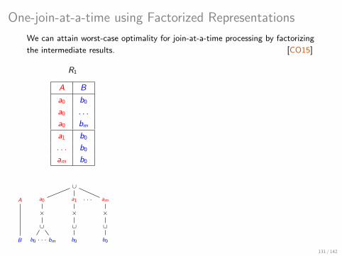

One-join-at-a-time using Factorized Representations
We can attain worst-case optimality for join-at-a-time processing by factorizing
the intermediate results. [CO15]
R1 R2
R3
A B
a0 b0
a0 . . .
a0 bm
a1 b0
. . . b0
am b0
A C
a0 c0
a0 . . .
a0 cm
a1 c0
. . . c0
am c0
B C
b0 c0
b0 . . .
b0 cm
b1 c0
. . . c0
bm c0
∪
a0 a1 . . . am
× × ×
∪ ∪ ∪
b0 . . . bm b0 b0
A
B
∪
a0 a1 . . . am
× × ×
∪ ∪ ∪
c0 . . . cm c0 c0
A
C
∪
b0 b1 . . . bm
× × ×
∪ ∪ ∪
c0 . . . cm c0 c0
B
C
131 / 142
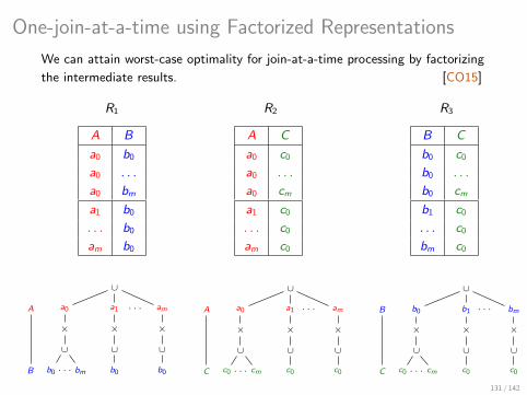
One-join-at-a-time using Factorized Representations
We can attain worst-case optimality for join-at-a-time processing by factorizing
the intermediate results. [CO15]
R1 R2 R3
A B
a0 b0
a0 . . .
a0 bm
a1 b0
. . . b0
am b0
A C
a0 c0
a0 . . .
a0 cm
a1 c0
. . . c0
am c0
B C
b0 c0
b0 . . .
b0 cm
b1 c0
. . . c0
bm c0
∪
a0 a1 . . . am
× × ×
∪ ∪ ∪
b0 . . . bm b0 b0
A
B
∪
a0 a1 . . . am
× × ×
∪ ∪ ∪
c0 . . . cm c0 c0
A
C
∪
b0 b1 . . . bm
× × ×
∪ ∪ ∪
c0 . . . cm c0 c0
B
C
131 / 142
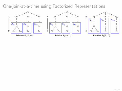
One-join-at-a-time using Factorized Representations∪
a0 a1 . . . am
× × ×
∪ ∪ ∪
b0 . . . bm
Ba0
b0
Ba1
b0
Bam
A
B
∪
a0 a1 . . . am
× × ×
∪ ∪ ∪
c0 . . . cm
Ca0
c0
Ca1
c0
Cam
A
C
∪
b0 b1 . . . bm
× × ×
∪ ∪ ∪
c0 . . . cm
Cb0
c0
Cb1
c0
Cbm
B
C
Relation R1(A, B). Relation R2(A, C). Relation R3(B, C).
∪
a0 . . . am
× ×
Ba0Ca0 Bam Cam
A
B C
∪
a0 a1 . . . am
× × ×
∪ Ca0
b0 . . . bm
Cb0Cbm
∪ Ca1
b0
Cb0
∪ Cam
b0
Cb0
A
B
C(R3)
C(R2)
∪
a0 a1 . . . am
× × ×
∪
b0 b1 . . . bm
× × ×
∪ ∪ ∪
c0 . . . cm c0 c0
∪
b0
×
∪
c0
∪
b0
×
∪
c0
A
B
C
After joining on A After joining on B After joining on C
m + 1 values 3m + 2 values 6m + 3 values
132 / 142
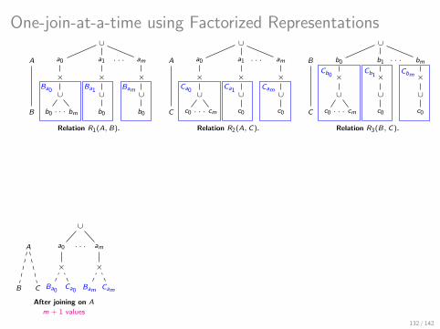
One-join-at-a-time using Factorized Representations∪
a0 a1 . . . am
× × ×
∪ ∪ ∪
b0 . . . bm
Ba0
b0
Ba1
b0
Bam
A
B
∪
a0 a1 . . . am
× × ×
∪ ∪ ∪
c0 . . . cm
Ca0
c0
Ca1
c0
Cam
A
C
∪
b0 b1 . . . bm
× × ×
∪ ∪ ∪
c0 . . . cm
Cb0
c0
Cb1
c0
Cbm
B
C
Relation R1(A, B). Relation R2(A, C). Relation R3(B, C).
∪
a0 . . . am
× ×
Ba0Ca0 Bam Cam
A
B C
∪
a0 a1 . . . am
× × ×
∪ Ca0
b0 . . . bm
Cb0Cbm
∪ Ca1
b0
Cb0
∪ Cam
b0
Cb0
A
B
C(R3)
C(R2)
∪
a0 a1 . . . am
× × ×
∪
b0 b1 . . . bm
× × ×
∪ ∪ ∪
c0 . . . cm c0 c0
∪
b0
×
∪
c0
∪
b0
×
∪
c0
A
B
C
After joining on A
After joining on B After joining on C
m + 1 values
3m + 2 values 6m + 3 values
132 / 142
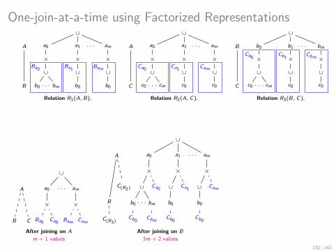
One-join-at-a-time using Factorized Representations∪
a0 a1 . . . am
× × ×
∪ ∪ ∪
b0 . . . bm
Ba0
b0
Ba1
b0
Bam
A
B
∪
a0 a1 . . . am
× × ×
∪ ∪ ∪
c0 . . . cm
Ca0
c0
Ca1
c0
Cam
A
C
∪
b0 b1 . . . bm
× × ×
∪ ∪ ∪
c0 . . . cm
Cb0
c0
Cb1
c0
Cbm
B
C
Relation R1(A, B). Relation R2(A, C). Relation R3(B, C).
∪
a0 . . . am
× ×
Ba0Ca0 Bam Cam
A
B C
∪
a0 a1 . . . am
× × ×
∪ Ca0
b0 . . . bm
Cb0Cbm
∪ Ca1
b0
Cb0
∪ Cam
b0
Cb0
A
B
C(R3)
C(R2)
∪
a0 a1 . . . am
× × ×
∪
b0 b1 . . . bm
× × ×
∪ ∪ ∪
c0 . . . cm c0 c0
∪
b0
×
∪
c0
∪
b0
×
∪
c0
A
B
C
After joining on A After joining on B
After joining on C
m + 1 values 3m + 2 values
6m + 3 values
132 / 142
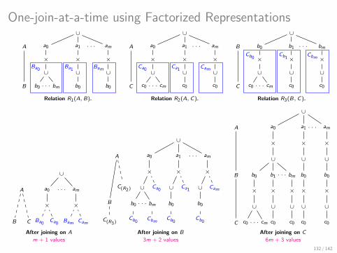
One-join-at-a-time using Factorized Representations∪
a0 a1 . . . am
× × ×
∪ ∪ ∪
b0 . . . bm
Ba0
b0
Ba1
b0
Bam
A
B
∪
a0 a1 . . . am
× × ×
∪ ∪ ∪
c0 . . . cm
Ca0
c0
Ca1
c0
Cam
A
C
∪
b0 b1 . . . bm
× × ×
∪ ∪ ∪
c0 . . . cm
Cb0
c0
Cb1
c0
Cbm
B
C
Relation R1(A, B). Relation R2(A, C). Relation R3(B, C).
∪
a0 . . . am
× ×
Ba0Ca0 Bam Cam
A
B C
∪
a0 a1 . . . am
× × ×
∪ Ca0
b0 . . . bm
Cb0Cbm
∪ Ca1
b0
Cb0
∪ Cam
b0
Cb0
A
B
C(R3)
C(R2)
∪
a0 a1 . . . am
× × ×
∪
b0 b1 . . . bm
× × ×
∪ ∪ ∪
c0 . . . cm c0 c0
∪
b0
×
∪
c0
∪
b0
×
∪
c0
A
B
C
After joining on A After joining on B After joining on C
m + 1 values 3m + 2 values 6m + 3 values
132 / 142

Open Problems for In-Database Optimization
133 / 142
Beyond the Current Setting
The presented framework works for semi-ring training expressions
Gradient computation and point evaluation are FAQ queries in the
sum-product semi-ring
Necessary for factorization
Beyond BGD: quasi-Newton, stochastic/coordinate GD
Further loss functions beyond square loss?
Further regularization functions beyond `2-norm?
Further ML problems typically used by LogicBlox
Decision/boosted trees, clustering, deep neural nets
Is the framework also applicable to these problems?
134 / 142

Effect of Functional Dependencies on Convergence
Rule: Eliminate features that are functionally determined.
It reduces
Computational complexity
Model complexity
Generalization error, i.e., how accurately an algorithm is able to predict
outcome values for previously unseen data.
Can it lead to faster BGD convergence?
How to approach non-linear dependencies?
Statistical effectiveness of above rule is difficult to gauge
Keep redundant variables if they help construct simpler
regression/classification functions
FD-aware optimizations beyond the `2-norm in the penalty term?
135 / 142
Foundations for In-Database Linear Algebra
Current research topic in the database systems community
Missing: Expressiveness and complexity analysis
For FD-aware model optimization, we need in-database support for
Tensor, Kronecker, Khatri-Rao products
Special cases of matrix inversion with rank-1 update, e.g.,
Sherman-Morrison-Woodbury
MS = I +∑s∈S
R>s Rs
as needed in the penalty term of the rewritten loss function:⟨(Icity + R>R)−1γcity,γcity
⟩Cholesky decomposition of matrices
Such linear algebra expressions can be phrased as queries in our framework.
136 / 142
Multi-Output Functional Aggregate Queries
Common ML tasks can be expressed as programs in languages with
functional aggregates and fixpoint.
These programs have many inter-related aggregates, e.g., σij and c .
Needed: Systematic investigation of algorithms and complexity for computing
large sets of inter-related aggregates.
Expected: Lower complexity that computing them independently.
137 / 142

Thank you!
138 / 142
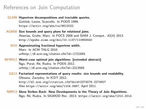
References on Join Computation
GLS99 Hypertree decompositions and tractable queries.
Gottlob, Leone, Scarcello. In PODS 1999.
https://arxiv.org/abs/cs/9812022
AGM08 Size bounds and query plans for relational joins.
Atserias, Grohe, Marx. In FOCS 2008 and SIAM J. Comput., 42(4) 2013.
http://epubs.siam.org/doi/10.1137/110859440
M10 Approximating fractional hypertree width.
Marx. In ACM TALG 2010.
urlhttp://dl.acm.org/citation.cfm?id=1721845
NPRR12 Worst-case optimal join algorithms: [extended abstract]
Ngo, Porat, Re, Rudra. In PODS 2012.
urhttp://dl.acm.org/citation.cfm?id=2213565
OZ12 Factorised representations of query results: size bounds and readability.
Olteanu, Zavodny. In ICDT 2012.
http://dl.acm.org/citation.cfm?doid=2274576.2274607
Also https://arxiv.org/abs/1104.0867, April 2011.
NRR13 Skew Strikes Back: New Developments in the Theory of Join Algorithms.
Ngo, Re, Rudra. In SIGMOD Rec. 2013. https://arxiv.org/abs/1310.3314
139 / 142
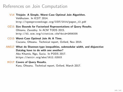
References on Join Computation
V14 Triejoin: A Simple, Worst-Case Optimal Join Algorithm.
Veldhuizen. In ICDT 2014.
http://openproceedings.org/ICDT/2014/paper_13.pdf
OZ15 Size Bounds for Factorised Representations of Query Results.
Olteanu, Zavodny. In ACM TODS 2015.
http://dl.acm.org/citation.cfm?doid=2656335
CO15 Worst-Case Optimal Join At A Time.
Ciucanu, Olteanu. Technical report, Oxford, Nov 2015.
ANS17 What do Shannon-type inequalities, submodular width, and disjunctive
Datalog have to do with one another?
Abo Khamis, Ngo, Suciu. In PODS 2017.
https://arxiv.org/abs/1612.02503
KO17 Covers of Query Results.
Kara, Olteanu. Technical report, Oxford, March 2017.
140 / 142

References on Aggregate Computation
BKOZ13 Aggregation and Ordering in Factorised Databases.
Bakibayev, Kocisky, Olteanu, Zavodny. In PVLDB 2013.
https://arxiv.org/abs/1307.0441
ANR16 FAQ: Questions Asked Frequently.
Abo Khamis, Ngo, Rudra. In PODS 2016.
https://arxiv.org/abs/1504.04044
141 / 142
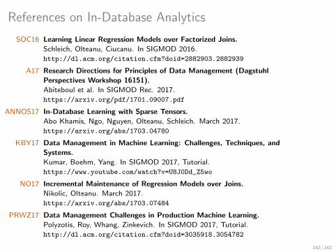
References on In-Database Analytics
SOC16 Learning Linear Regression Models over Factorized Joins.
Schleich, Olteanu, Ciucanu. In SIGMOD 2016.
http://dl.acm.org/citation.cfm?doid=2882903.2882939
A17 Research Directions for Principles of Data Management (Dagstuhl
Perspectives Workshop 16151).
Abiteboul et al. In SIGMOD Rec. 2017.
https://arxiv.org/pdf/1701.09007.pdf
ANNOS17 In-Database Learning with Sparse Tensors.
Abo Khamis, Ngo, Nguyen, Olteanu, Schleich. March 2017.
https://arxiv.org/abs/1703.04780
KBY17 Data Management in Machine Learning: Challenges, Techniques, and
Systems.
Kumar, Boehm, Yang. In SIGMOD 2017, Tutorial.
https://www.youtube.com/watch?v=U8J0Dd_Z5wo
NO17 Incremental Maintenance of Regression Models over Joins.
Nikolic, Olteanu. March 2017.
https://arxiv.org/abs/1703.07484
PRWZ17 Data Management Challenges in Production Machine Learning.
Polyzotis, Roy, Whang, Zinkevich. In SIGMOD 2017, Tutorial.
http://dl.acm.org/citation.cfm?doid=3035918.3054782
142 / 142
Related Documents

![[123doc.vn] - kinh-nghiem-thi-tuyen-dung-cua-cong-ty-samsung-duoc-chia-se-tren-cac-dien-dan.pdf](https://static.cupdf.com/doc/110x72/577c7dae1a28abe0549f8f3a/123docvn-kinh-nghiem-thi-tuyen-dung-cua-cong-ty-samsung-duoc-chia-se-tren-cac-dien-danpdf.jpg)