Damage model for brittle elastic solids with unequal tensile and compressive strengths

Pergamon

Engineering Fra~~rure Mechrmic.~ Vol. 49. No. 5. pp. 6XlH97. 1994 Copyright ‘c 1994 Elsevier Science Ltd

0013-7944(94)00183-9 Printed in Great Britain. All rights reserved 0013-7944:94 $7.00 + 0 00

DAMAGE MODEL FOR BRITTLE ELASTIC SOLIDS WITH

UNEQUAL TENSILE AND COMPRESSIVE STRENGTHS

V. A. LUBARDA, D. KRAJCINOVIC and S. MASTILOVIC

Department of Mechanical and Aerospace Engineering, Arizona State University, Tempe, AZ 85287-6106, U.S.A.

Abstract-The paper presents a rate-type constitutive analysis of damage, applicable to brittle materials whose elastic properties degrade during a deformation process. Different tensile and compressive material responses are modeled incorporating positive and negative projections of the stress or strain tensors. Proposed evolution laws for the rate of compliance tensors are consistent with some of the prominent features of brittle material response. A new structure of the damage surface is introduced for a more accurate account of the effects of the hydrostatic states of stress on the overall response. Derived rate constitutive equations provide the explicit representation of the tangent compliance tensor. The proposed model is applied to uniaxial tension and compression to illustrate nonlinear relationships between stress and longitudinal, lateral, and volumetric strains. The proposed model is compared with some of the existing theories.

1. INTRODUCTION

DEGRADATION of elastic properties reflecting accumulating damage in brittle materials is primarily a consequence of the evolution of internal microcrack structure. Depending on the material microstructure and the current state of stress and strain and their rates, instantaneous material response and further evolution of damage may involve activation of different microcrack mechanisms. The tensile hoop stress generated at the surface of relatively large pores represents a preferential crack nucleation mechanism in very porous rocks. In low porosity, compact rocks frictional sliding of crack surfaces can destabilize original shear cracks, causing them to kink and develop wing cracks. Other mechanisms of microcracking are also possible. Some of these mechanisms were implemented in the failure analysis of brittle solids by Ashby and Sammis [I],

and others. Progressive degradation of mechanical properties is an inherent feature of brittle material

behavior. Several analytical models were developed to estimate the effective elastic properties of a solid weakened by a given distribution of microcracks or other defects. A comprehensive review of these models can be found in a recent treatise by Nemat-Nasser and Hori [2]. An important issue in the formulation of continuum damage models is related to the appropriate choice of the mathematical form for the damage variable. This has been recently studied by Lubarda and Krajcinovic [3], who considered several frequently encountered two and three dimensional distri- butions of microcracks. Their analysis demonstrated the shortcomings of the scalar and second- order tensor damage variables, and the accuracy gained by using the fourth-order tensor variable.

The mode and stability of crack growth and, therefore, behavior of brittle material strongly depends on the sign and magnitude of applied stresses. For instance? the response of brittle material subjected to a compressive loading is strongly dependent on the magnitude of lateral confinement. An unconfined specimen fails by axial splitting, attributed to unstable growth of a single crack, at relatively small microcrack density. As the confinement is increased, axial splitting is suppressed and at large levels of confinement homogeneous microcracking prevails throughout the sample, resulting in a quasi-ductile overall response (Horii and Nemat-Nasser [4]).

The analysis presented in this paper addresses the important issue of modeling different tensile and compressive responses of brittle materials. The concept of positive and negative projections of stress and strain tensors is used to account approximately for two basic, tensile and compressive, damage evolution modes. This idea was independently introduced by Ladeveze and Lemaitre [5], Ortiz [6] and Mazars [7], and was subsequently utilized by Simo and Ju [8], Yazdani and Schreyer [9], Ju [IO], Stevens and Liu [l 11, Yazdani [12], and others. The positive parts of the stress

681

682 V. A. LUBARDA et al

and strain tensors are obtained by using the positive stress and strain projection operators P,’ and P;‘. When applied to stress c and strain c tensors, these operators remove their negative eigenvalue components

G+=P;:b, L’=P::c. (1)

In (I), the symbol (:) denotes the trace product of the fourth-order projection operator and the second-order tensor. If ny) and ny) (c( = 1,2, 3) are the three orthogonal principal directions of the stress and strain tensors, respectively, the corresponding positive projection operators are defined by

In (2) and (3), G(‘) and c@) are the principal stress and strain components, while the angular brackets are defined such that

((1) = -c 1, n>,O

0, a<0

for any scalar a. The remaining parts of the stress and strain tensors are their negative parts

Substituting eq. (1) into eq. (5), it follows

6 ==P,:c, t- =P<-:t, (6)

where

P, =1--p;, P; =1-P’ < . X7)

In eq. (7), I denotes the fourth-order identity tensor. In general, for elastically anisotropic and, for certain states of stress and strain, even elastically isotropic materials, P,* # P: and P; +P, . The symmetry properties of the projection operators, in particular the reciprocal symmetry P,, = Pklijt hold for positive and negative stress and strain projection operators. A proper de~nition of the projection operators is discussed in more detail in the Appendix to this paper.

The rate theory of damage elasticity presented in this paper is based on the assumption that no residual strain is left upon unloading to zero stress from any state of deformation. The analysis is a generalization of previous work by the same authors (Lubarda and Krajcinovic (131). introduced to model different tensile and compressive responses of brittle materials. Basic formulation is provided in stress space, with a straightforward extension to strain space. The suggested rate (evolution) expressions for the compliance fluxes are in accord with some of the essential features of the experimentally observed brittle response. Damage surface is defined and the rate-type constitutive equations formulated. Explicit representation of the tangent compliance tensor is also given. Several important applications are discussed, and results are compared with a related work.

Incorporation of residual (plastic) strains into the constitutive framework and the finite strain aspects of the analysis are left for a forthcoming paper.

2. PRELIMINARY ANALYSIS

Consider small defo~ations of brittle material whose elastic properties change during a deformation process. Assume that the residual strain vanishes upon unloading initiated from an arbitrary state of deformation. Degradation of elastic properties is attributed to the accumulated damage, i.e. nucleation and propagation of microcracks during a deformation process. Let 8:. denote the surface energy of the microcrack surfaces created in the course of deformation from

Damage model for brittle elastic solids 683

the initial to the current state. The Helmholtz free energy @ and the Gibbs energy II/ (per unit

volume) can then be defined as

@ =$?(@E)+&; (8)

Y =+%?(a@a)-E;., (9)

where c and c are the stress and strain tensors, and 2 and &the current elastic stiffness and compliance tensors. The symbol (:) stands for the inner, trace product and 0 for the outer tensor product. As discussed in the context of the thermodynamic analysis of the quasi-static growth of Griffith cracks (Rice [14]), free energy at the current state is equal to the work done in transforming the body from its initial to current state along an imagined reversible and isothermal path. This path can be recreated by a sequence of two steps. First, new microcrack surfaces are formed separating reversibly the adjacent layers of atoms, pulling against their cohesive forces. The work needed to overcome cohesive forces is denoted by E:.. Second, the microcracked solid is deformed elastically to the current state of deformation c. The required work is ;Z: (c 0 t), where dp denotes the current elastic stiffness which accounts for the presence of all existing active cracks. A microcrack is considered to be active if it imposes a discontinuity in at least one component of the displacement vector across its surface. Lubarda and Krajcinovic [l3] have presented a constitutive analysis of damage behavior in brittle elastic solids by using both, elastic stiffness and elastic compliance tensors. In this section we rederive some of these results, restricting for brevity the attention to formulation based on the Gibbs energy and the elastic compliance tensor.

Since elastic compliances increase as damage evolves, it is convenient to represent the current elastic compliance tensor &‘in an additive form

dt=~&+M, (10)

where 4 denotes the initial elastic compliance tensor of the undamaged material. The fourth-order tensor &can be considered as being an appropriate measure of the accumulated damage. This tensor changes during a deformation process as a consequence of the material degradation, i.e. the nucleation of new and the growth of existing microcracks. The rate of the Gibbs energy is obtained by differentiating eq. (9)

@ =~:(aOs)+ni:f(aob)--;. (11)

The reciprocity symmetries of the tensor &are used in arriving at eq. (11). From the first law of thermodynamics, the rate of Gibbs energy in an isothermal deformation process is

!I+ = t :& + TA, (12)

where T is the temperature, and n the irreversible entropy production rate. The product TA represents the energy dissipation rate associated with the damage evolution. As a consequence of the second law of thermodynamics, n 3 0. Comparing eqs (1 I) and (l2), it follows that

IZ =&%?:a (13)

TA = n;l:;(c~ @a) - 6,. (14)

Equation (13) is the elasticity equation relating the current stress and strain tensors through the current elastic compliance tensor A= 2-l. Equation (14) gives the energy dissipation rate, written in terms of the stress tensor b, and the damage flux Ri. Indeed, introducing

r =+ @a), (15)

as the thermodynamic force (affinity) conjugate to damage tensor M, eq. (14) can be written as

TA = r : k - 6;. (16)

The affinity f was previously utilized in the literature by Ortiz[6], Simo and Ju [8], Ju [lo], Krajcinovic et al. [15], and others.

684 V. A. LUBARDA ef al.

Suppose that there is a scalar function C2 = R(T) such that the damage flux !$I can be expressed as

where p is the rate of some monotonically increasing scalar parameter p, which can be considered as being a measure of the cumulative damage at the considered state. Hence, in absence of healing, fi > 0. The function R is referred to as a damage potential for the flux &I. Substituting eq. (17) into eq. (16), the energy dissipation rate can be expressed as

If 0 is a homogeneous function of r of degree n, eq. (18) reduces to

T/l =pnR-C.,. (19)

Since the energy dissipation rate is non-negative, from eq. (19) it follows

,&!5 >o, dp ’

(20)

The equality sign in eq. (20) applies only if all energy associated with the damage process is transformed into the surface energy of the created microcrack faces.

The expression for the strain rate can be derived differentiating eq. (13) and using eq. (ICI).

i = .&& +M:a. (31)

The first term on the right-hand side of (21) is the strain rate that would correspond to stress rate t? if the damage flux M would be zero. This part of the strain rate is referred to as the elastic part of the strain rate. The remaining part

id=M:c (22)

is the strain rate attributable to change in damage, referred to concisely as the damage strain rate. Substituting eq. (17) into eq. (22)

i.e.

JR [“=P,-.

ca (24)

Therefore, the damage potential R serves as a dual potential: for the damage flux !%‘I in the space of affinity r, i.e. eq. (17), and for the damage strain rate L *’ in the space of stress 0, i.e. eq. (24).

3. UNEQUAL TENSILE AND COMPRESSIVE STRENGTHS

Since the compliance flux M is primarily a consequence of the stress-induced evolution of internal crack structure, and is strongly dependent on the sign of applied normal stresses (tensile or compressive), it is assumed that the flux M consists of two parts, such that

M=M++M. (25)

The flux M+ contributes to “positive” part of the compliance tensor M+, activated by a positive part of the stress tensor a +, while M- contributes to “negative” part of the compliance tensor M ,

activated by a negative part of the stress tensor u _. The total strain is then determined from

t=,,&:a+M+:a++M~:a (26)

The representation (26) correctly predicts (to a certain extent) the so-called unilateral damage effect (Lemaitre [16], Chaboche [ 171) i.e. a sudden stiffening and recovery of the elastic properties due

Damage model for brittle elastic solids 685

to the crack closure which occurs during reloading in compression, following a previous tension loading.

Consider the following structure of the damage potential

n=d:r, d= i f_ auNi@Nj. !=I j=l

(27)

In (25) a,, are the constants (a,, = ail) and

Ni= ni@n, (i = 1, 2, 3) (28)

are the dyadic products of the eigendirections nj of the stress tensor 6. Consequently

(29)

and the flux l$l, defined by eq. (17), becomes

ni=p&L (30)

To express the flux, eq. (30), in the additive form, eq. (25) the tensor & is written as

Az=&++L&. (31)

The positive and negative contributions to & depend on the current state of stress in the following

manner. Denote the principal stresses by cr, , o2 and o3 (g, 2 g2 2 g3). If all three principal stresses are different (a, # cr2 # a,), it is assumed that:

&+ = c[N, 0 N, + a(N) 0 N3)s]

d- =N,ON,+b(N,ON,),, (32)

where the subscript s denotes the symmetric part. Constants a, b and c play the role of material parameters, and are specified according to experimental data. The parameter c is related to the ratio of material strengths in tension and compression, while a and b are specified according to observed lateral strain-longitudinal stress response, as discussed in Section 6. The parameters a and b may be appropriate constants or, more generally, functions of the hydrostatic part of stress tensor. The structure (32) is constructed in accordance with experimentally observed feature of brittle material response, which indicates that cracks dominantly propagate in planes normal to the direction of largest principal stress. In the case of equal magnitudes of certain principal stresses, the following modifications are suggested. If the principal stresses are such that 0, # crz = cr3, eq. (32) is replaced by

(33)

d- =N,ON,+~[(N,~N,),+(N,~N,),l. (34)

Finally, in the case of the spherical state of stress cr, = g2 = c3, the suggested expressions for the positive and negative parts of the tensor L& are

&- =‘I 3 3

where I = N, 0 N, + N, 0 N, + N3 0 N, is the fourth-order unit (identity) tensor.

(35)

686 V. A. LUBARDA et al.

The advantages of the proposed evolution laws for the compliance fluxes are evident from discussions in Section 6, demonstrating the capability of the proposed equations to capture essential nonlinear features of uniaxial stress vs longitudinal, lateral, and volumetric strain behavior. Naturally, the proposed model is not without flaws. For example, if the previous loading history was such that damage consists of cracks created dominantly in the planes parallel to a given direction (say, longitudinal direction in the case of uniaxial compression), reloading and subsequent loading in triaxial tension would likely cause further crack growth in the same planes. Equation (35), however, indicates an isotropic increment of the damage evolution. The same flaw, however, is shared by other damage models, such as one proposed by Ortiz 161.

4. DAMAGE SURFACE

To distinguish between the unloading-elastic behavior and loadingdamage behavior, introduce a damage function in stress space Z(a+, IS .-), which depends on both positive and negative parts of the stress tensor (defined in the Introduction to this paper), such that the locus of points

Z(c+, 0 )-R(p)=% (36)

encloses the stress region within which the response of material is purely elastic. The surface defined by (36) is referred to as a damage surface in stress space. The parameter R, which defines the size of the surface, is assumed to depend on the cumulative damage parameter p. The representation (36) is the simplest version of the damage criterion. It implies that during damage evolution initial damage surface expands isotropically in stress space and that its evolution is fully defined by a single scalar. This is often not a satisfactory assumption, particularly for nonproportional loading paths. For example, loading in uniaxial compression beyond the initial damage threshold creates microcracks that are likely to remain inactive upon unloading and subsequent reverse loading in tension. Hence, while the damage threshold stress is increased during compression, it remains virtually unchanged for a reverse loading in tension, until the tensile loading creates additional damage by itself. Therefore, isotropic evolution of the damage surface cannot be expected to work well in non-proportional loading. This is analogous to the isotropic hardening models used in metal plasticity. In the present case the situation is further exacerbated by the dependence of the damage evolution on the sign of the normal stress. The tendency for localized change in shape of the damage surface during certain loading paths has been discussed by Holcomb and Costin [18].

If the stress state is on the damage surface, the subsequent stress state will also be on the damage surface, provided that the consistency condition is satisfied

ac ac dR ~:6++-:6 --

au- dp P = 0.

From eq. (37), the rate of the cumulative damage parameter is

.iac - P=h abf.0

i . .++g:y ) u 1

(37)

(38)

where h = dR/dp. Since progressive damage implies p > 0, from eq. (38) follows that during the damage loading

(39)

In the hardening regime (h > 0), eq. (39) represents the damage loading condition. However, in the softening regime (h < 0), the condition

(40)

represents only a necessary but not sufficient condition for the damage loading, since the inequality (40) can be satisfied during elastic unloading as well.

Damage model for brittle elastic solids 687

Note that C(a ‘, 6 -) = C(P+ : CT, P- : G), but ;I # (8 X/&J) : 6, since P+ and P- are not constant operators. Consequently, the last expression in (3.64) and expressions (3.66) of the Ortiz [6] paper apply ifa+:+ =~~:4+ =O, i.e. if the projection operators P+ and P- are constant operators.

Consider the damage function of the form analogous to that of Ortiz [6], i.e.

C =ikb+:a+ +~a~:a-, (41)

where the material parameter k (the cross-effect coefficient) is specified to reflect unequal strengths in tension and compression. The rate of change of the cumulative damage parameter eq. (38) is in this case

p = k (ka +:c?+ +a-:&). (42)

Yazdani and Schreyer [9] and Yazdani [12] used more involved representations of the damage surface to remove some of the perceived deficiences associated with eq. (41). For example, if the damage threshold stress in uniaxial compression is ai-, (41) predicts that the damage threshold stress under hydrostatic compression is a; /$. However, experimental evidence indicates that little or no damage is observed under hydrostatic compression alone. A plausible modification of eq. (41) to provide a more accurate estimate of the effect of the hydrostatic pressure is

C =;k[S+:S+ +a(p+)*]+;[S- :S- +fi(pm)2]. (43)

where S’ = a* +p’6 are the deviatoric parts of the positive and negative parts of the stress a?, + p - = - fa * : 6 are the corresponding hydrostatic pressures (6 denotes the second-order unit tensor),

while ~1, p and k are material parameters, specified in accordance with the experimental data. Let the damage threshold stress in uniaxial compression be a;, and in uniaxial tension 0:. If the damage threshold stress under hydrostatic pressure is p;, and under hydrostatic tension PO+, it can be shown that

’ (45)

where 9 =~;/a; and 9+ =po+/a,+. The rate of change of the cumulative damage parameter, eq. (38), corresponding to the damage function, eq. (43), is

fi =; [k(S+ -$xp+ s):&+ +(S- -fPpma):q.

If c1 = /3 = 3, eq. (46) reduces to eq. (42). It can be easily shown that in the case of uniaxial compression, the damage parameter p is equal to (E-’ - Et’), where E is the current degraded elastic (secant) modulus, appearing in the uniaxial compression stress-strain relationship CJ = E(c)c,

and E,, is the initial elastic modulus. The parameter R is equal to h(6 + p)02. Consequently, the relationship R = R(p) can be easily extracted from the given compression stress-strain relationship (T = E(E)L. If the tension stress-strain curve is used, the parameter R is equal to (k/18)/6 + c( (02,

while the damage parameter p is equal to c-‘(Em’ - E;‘), where E is the current degraded elastic (secant) modulus in the uniaxial tension test. Other applications are considered in Section 6 of this paper. The selection and the significance of the appropriate structure of the damage surface is further discussed by Lubarda and Krajcinovic [13]. Important related issues were also studied by Holcomb and Costin [ 181, and Ashby and Sammis [I].

5. COMPLETE RATE-TYPE CONSTITUTIVE EQUATIONS

The rate of the total strain is derived by differentiating the stress-strain relationship, eq. (26),

i=(~&+M+):&++(.4&~+M~):&+I\i+:a++I\i-:a-. (47)

688 V. A. LUBARDA et al.

In eq. (47),

i’=(&+M+):ti+ +(&+M-):S-, (48)

is recognized as the elastic part of the strain rate, while the remaining part

[d=l\jl+:ut +l\;I- :*- (49)

is the damage strain rate. The evolution equations for the positive and negative compliance fluxes are obtained from eqs (30) and (31) as

M+ = p&J+, 1\;1- = pa-. (50)

Using the previously derived expression for the rate of the cumulative damage parameter p, the damage strain rate (49) becomes

id=; [(*@++ +(&+I. (51)

In eq. (51), the second-order tensor A stands for

A=d+:a++& :C (52)

Therefore, the eq. (47) for the total strain rate becomes

i =&:~++&-:(j~ (53)

where .Y&+ and & are the “positive” and “negative” tangent compliance tensors, given by

(54)

Equation (53) represents the overall rate-type constitutive relation for the damage response of brittle elastic solids with unequal tensile and compressive strengths.

It is pointed out that for the prescribed stress rate d, the positive part of the stress rate appearing in the above equations is defined by

&+=lim P:+a,:(6 +d At)--;:a

At Al-0 (55)

The negative part of the stress rate is defined by an analogous expression. For the damage function prescribed by (43), the overall rate-type constitutive equation takes

the form

i= &+M++;A@(S+ [

-;ccp+~S) 1 i

:d+ + &+M- +; A@(S- -f&-6) 1 :C. (56)

Equation (56) is the specific representation of the general expression (53), corresponding to the selected damage function, eq. (43).

Other representations of the damage function can be constructed and incorporated into the presented constitutive framework, along the lines suggested by Lubarda and Krajcinovic [13]. Numerical implementation of the constitutive equations, such as eq. (53) or its special form eq. (56), corresponding to a selected representation of the damage function, is analogous to that of the familiar rate-type plasticity theory. The same applies to the corresponding constitutive structures of

Damage model for brittle elastic solids 689

the strain space formulation. Some of the computational aspects of other formulations have already been addressed in the damage mechanics literature, for example by Simo and Ju [19] and Ju [lo].

6. APPLICATIONS

6.1. Specifications of material parameters

The material parameters introduced in the above formulated model are specified according to experimental data measured for Salem limestone by Green [20]. In the uniaxial compression test (without confinement), the first significant departure from linearity of the stress-strain relationship is observed at the stress level of about a; = 60 MPa, and the corresponding strain level

- = 1.6 x 10m3. The initial elastic modulus is, therefore, calculated to be E, = 37.5 GPa. The Fiilure occurred at the stress level of about 69 MPa, and the corresponding strain of 2.1 x 10-j. The experimental data in uniaxial tension show more pronounced, specimen dependent scatter. The failure stress ranges from 5 to 6 MPa, so that the average ratio of the compressive to tensile strengths is 69/5.5 z 12.5. The tensile damage threshold stress oz is not easily identified, and in calculations performed herein it is assumed that the ratio a;/o,i is also equal to 12.5, so that ol = 4.8 MPa. The initial elastic modulus in tension is taken to be the same as in compression, i.e. E, = 37.5 GPa. In absence of triaxial tension data, it was further assumed that the hydrostatic damage threshold in tension is pi = CT:,/&. Since brittle materials can sustain a much higher hydrostatic pressure, it is taken that p; = IOcr;. Consequently, the parameters rr, p and k, defined by eqs (44) and (4.5), have the following numerical values

c1=3, /I+, kzlO4. (57)

The initial damage criterion, C = R,, with the damage function Z defined by eq. (43): and with R,, = (6 + ~)(~~)*/18, is represented for a biaxial state of stress (ci3 = 0) in Fig. 1.

Fig. 1. Damage criterion for biaxial state of stress corresponding to damage surface eq. (43) and material parameters specified by eq. (57). The damage onset stress in uniaxial compression UC is 12.5 times that

in uniaxial tension CT:.

690

U-[ MPa] 801

V. A. LUBARDA et al.

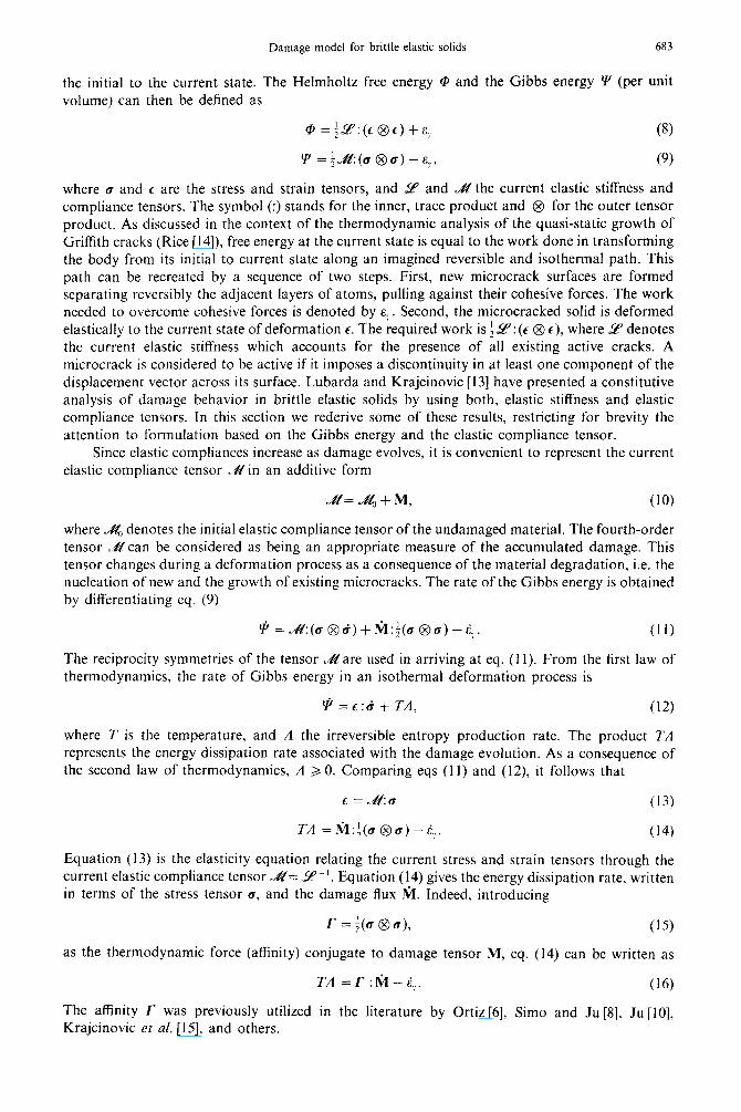
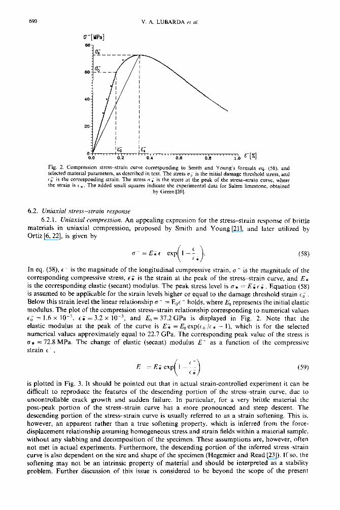
c- [x] Fig. 2. Compression stress-strain curve corresponding to Smith and Young’s formula eq. (58) and selected material parameters, as described in text. The stress 00 is the initial damage threshold stress, and 6; is the corresponding strain. The stress a; is the stress at the peak of the stress-strain curve, where the strain is cj. The added small squares indicate the experimental data for Salem limestone, obtained

by Green [20].

6.2. Uniaxial stress-strain response

6.2.1. Uniaxial compression. An appealing expression for the stress-strain response of brittle materials in uniaxial compression, proposed by Smith and Young [21], and later utilized by Ortiz [6,22], is given by

u- =Ezc- exp (58)

In eq. (58), L is the magnitude of the longitudinal compressive strain, rr is the magnitude of the corresponding compressive stress, cz is the strain at the peak of the stress-strain curve, and ES

is the corresponding elastic (secant) modulus. The peak stress level is cr ; = E; L & Equation (58) is assumed to be applicable for the strain levels higher or equal to the damage threshold strain c0 . Below this strain level the linear relationship ~7 - = E,t ~- holds, where E,, represents the initial elastic modulus. The plot of the compression stress-strain relationship corresponding to numerical values

60 = 1.6 x 10m3, c; = 3.2 x 10e3, and EO = 37.2 GPa is displayed in Fig. 2. Note that the elastic modulus at the peak of the curve is E; = E,exp(c;/c; - I), which is for the selected numerical values approximately equal to 22.7 GPa. The corresponding peak value of the stress is B* = 72.8 MPa. The change of elastic (secant) modulus E- as a function of the compressive strain c-,

is plotted in Fig. 3. It should be pointed out that in actual strain-controlled experiment it can be difficult to reproduce the features of the descending portion of the stress-strain curve, due to uncontrollable crack growth and sudden failure. In particular, for a very brittle material the post-peak portion of the stress-strain curve has a more pronounced and steep descent. The descending portion of the stress-strain curve is usually referred to as a strain softening. This is, however, an apparent rather than a true softening property, which is inferred from the force- displacement relationship assuming homogeneous stress and strain fields within a material sample, without any slabbing and decomposition of the specimen. These assumptions are, however, often not met in actual experiments. Furthermore, the descending portion of the inferred stress-strain curve is also dependent on the size and shape of the specimen (Hegemier and Read [23]). If so, the softening may not be an intrinsic property of material and should be interpreted as a stability problem. Further discussion of this issue is considered to be beyond the scope of the present

Damage model for brittle elastic solids 691

paper. Some of the representative references to strain softening, its relation to localization, length scale and size effect, and other pertinent issues, are Baiant [24], Baiant et al. [25], Read and Hegemier [26], Schreyer and Chen [27], Needleman [28], and Karihaloo et al. [29]. Integrating (.50), and in view of (26) and (34)2, one has

1 c- = ( > E;,+p c-.

Hence, since cr --/c ~ = E- is the current value of the longitudinal elastic modulus, the expression for the cumulative damage parameter can be derived from (60) as

In particular, the value of p at the peak of the stress-strain curve is obtained from I&p* = E,/E; - 1, which gives p* = 0.649B;‘. It is easy now to rewrite eq. (58) in the parametric form as

t- =c* l+ln-i*) ( 0 *

(r -. 1 +Eop*

=O* 1+&J&I I+ln I+“’ ~-

1 +a!+* I. (62)

The parameter R, which defines the size of the damage surface eq. (36), can be expressed by using eq. (43) as

R =$(~-+-P)(G-)~. (63)

The relationship R = R(p) is obtained substituting (62& into (63) and is plotted in Fig. 4. 6.2.2. Uniaxiaf tension. By an analogous procedure, in the case of uniaxial tension it follows

that

R =+(6+z)(cr+)’ (64)

E- [CPa] 40-

:%

30 -

zo-

lo-

o (,,I,,/,,,),,,,,,,I,,,,,,,,rl,l,,,I,,,

0 0.2 0.4 0.6 TB WI

Fig. 3. The change of elastic (secant) modulus E in uniaxial compression as a function of strain 6 -, according to eq. (59). E0 is the initial elastic modulus of undamaged material.

692 V. A. LUBARDA et al.

R (Io'(Ypa)*)

0.0 ~,,,.,,.,,,,,,,.,,..,,,,,,,,,,,,,,.,,..,,,,,.,,,.. 0 2 3 1 4 A&P

Fig. 4. The change of parameter R, which defines the size of damage surface, as a function of non-dimensional cumulative damage parameter E,p. R, is the initial damage threshold value of R. at

p =o.

The tensile stress CY+ can be expressed as a function of the damage parameter p by equating eqs (63) and (64). This gives

CT+=lS*+ 1 + E,p* 1 +EOP 1 +EOP

1 +ln > 1+&p* ’

where

(66)

is the stress at the peak of the tensile stress-strain curve. For assumed values of the parameters CI, p and k, given by eq. (57) the coefficient K is equal to the reciprocal of 12.5, which is also equal to the previously assumed value of the stress ratio ~$/a;. Since L+ = cr+/E+, it follows that

t+ =.C*+ l+cEop 1 +Eop*

1 + cEop* I+ Eop

where

C$ =K 1 $-c&p* _

1 + Eop* ‘*

(68)

is the strain at the peak of the tensile stress-strain curve. The parameter c, appearing in eqs (65)-(69), is specified by requiring that the strain at the peak

of the tensile stress-strain curve is l/l0 of the strain at the peak of the compressive stress-strain curve. This is in agreement with the experimental data on Salem limestone (Green [20]). From (69) therefore,

1 c =-

EOP* K-‘(1 +E,p+ 1 (70)

For the considered numerical values, from eq. (70) c = 1.635. Experimental data on concrete indicate higher values of the ratio L 5 /c ; , and l/5 would be a reasonable estimate. The plot of the tensile stress-strain curve d + = CJ +(c +), corresponding to eqs (66) and (68), is shown in Fig. 5.

Damage model for brittle elastic solids 693

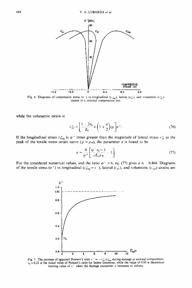
6.3. Lateral strain behavior 6.3.1. Uniaxial compression. The lateral strain in the direction normal to the longitudinal

compressive direction is obtained from eqs (26) (34), and (50),

(71)

where ~1” is Poisson’s coefficient of the undamaged material. The initial value of Poisson’s ratio for the Salem limestone is v0 z _ 0.22. The volumetric strain is then

c,,= -[!z$+(l +g+ (72)

The material parameter b is specified by requiring that the magnitude of the longitudinal strain

clone is cp times greater than that of the lateral strain ~,,t at the peak of the stress-strain curve. From this condition

(73)

For example, for cp = 2, and for the selected numerical values, eq. (73) gives b z - 3.72. Diagrams of the compressive stress (a-) vs longitudinal (t,& = --t -), lateral (tla,), and volumetric (t”;,) strains are displayed in Fig. 6. Note that for cp = 2, the volumetric strain vanishes at the peak of the stress-strain curve. Observe the dilatant volume increase which occurs as a consequence of the microcrack growth and opening under compressive load, so that the volumetric strain changes from compressive to tensile. The increase of apparent Poisson’s ratio

6 I,1 vm = --= v. - 0.25bEop

6 long l+E,p ’ (74)

as a function of E,,p is given in Fig. 7. The limiting value of v -, as E decreases to zero or p tends to infinity. is equal to -b/4.

6.3.2. Uniaxial tension. The lateral strain in the case of uniaxial tension is

U+[ MPa]

6- _-_---- - c

I

0 I I

-0; , I

I 4-

2 II,, 8.00

I % It: 0.02 0.04 0.00 0.08 0.10 0.12

(75)

&+[%I

Fig. 5. Tension stress-strain curve whose parametric representation is given by eqs (66) and (68). The stress 0,’ is the initial damage threshold stress, and c$ IS the corresponding strain. The stress ut is the stress at the peak of the stress-strain curve, where the strain is t $. The added small squares indicate the

experimental data for Salem limestone, obtained by Green [20].

694 V. A. LUBARDA et al.

(T-[MPa]

COMPRESSIVE STRAIN [X]

Fig. 6. Diagrams of compressive stress (u ) vs longitudinal (c&), lateral (TV,), and volumetric (C ,,) strains in a uniaxial compression test.

while the volumetric strain is

CL, = [?+(I +$++. (76)

If the longitudinal strain c,& is cp + times greater than the magnitude of lateral strain c,:, at the peak of the tensile stress-strain curve (p = p*), the parameter a is found to be

For the considered numerical values, and the ratio cp + = 6, eq. (77) gives a z -0.464. Diagrams of the tensile stress (G+) vs longitudinal (c& = t +), lateral (t&), and volumetric (c,‘,,) strains are

v- 1.0

0.93 t---------------------

0.6 ;

0.6 :

0.4 -

0.2 1 vo

Fig. 7. The increase of apparent Poisson’s ratio B - = --t ,;,/r lone during damage in uniaxial compression. v0 = 0.22 is the initial value of Poisson’s ratio for Salem limestone, while the value of 0.93 is theoretical

limiting value of v- when the damage parameter p increases to infinity.

Damage model for brittle elastic solids 695

a+[ MPa] -6

TENSILE STRAIN [X]

-0.01 0 0.01 0.02 0.03 0.04 0.05 0.06

Fig. 8. Diagrams of tensile stress (u ‘) vs longitudinal (t ,&), lateral (6 I:,) and volumetric (6 $,) strains in a uniaxial tension test.

shown in Fig. 8. The dilatation effects under tension load are far less pronounced than in compression, and the volumetric strain is always tensile. The decrease of apparent Poisson’s ratio

v+ - c t vO - 0.25acE,p

- --= 6 Iing 1 + cEop

as a function of E,p is given in Fig. 9. The limiting value of v+, as p goes to infinity, is equal to -a/4.

7. CONCLUSION

The analysis presented in this paper provides the rate-type constitutive equations for elastic behavior of brittle material, whose elastic properties degrade during a path-dependent deformation process involving damage evolution. A marked difference in brittle material response dependent on the sign of applied normal stresses (tensile or compressive) is modeled by introducing positive and negative stress and strain operators. The basic formulation is presented in stress space, with

0.0 ,111,11’,1,‘.1111111,,,,,~,,,~,,,,,,,,,,,,,,,,,,~~ c&J 0 1 2 3 4 5

Fig. 9. The decrease of apparent Poisson’s ratio Y + = --C&/C + long during damage in uniaxial tension. rg = 0.22 is the initial value of Poisson’s ratio for Salem limestone, while the value of 0. I 16 is the theoretical

limiting value of v+ when the damage parameter p increases to infinity.

696 V. A. LUBARDA er al.

a straightforward extension to strain space. Proposed representation of the evolution equations for the compliance fluxes is in accord with some of the basic features of the experimentally observed brittle material response. The rate-type constitutive equations are derived by using a new, physically appealing structure of the introduced damage surface. By virtue of its incremental nature, the presented phenomenological analysis is capable of modeling the path-dependent degradation of elastic properties and induced elastic anisotropy. Applications to uniaxial tension and compression lead to experimentally observed relationships between the stresses and the longitudinal, lateral and volumetric strains.

The applicability of the results presented in this paper will be significantly extended when the residual or plastic strains are adequately incorporated in the proposed constitutive framework. Residual strains inevitably arise during deformation, because upon unloading the cracks are prevented to return to their original configurations due to misfits, interlocks, and other geometric and kinetic effects of the interacting crack population. Furthermore, since brittle materials can exhibit significant apparent ductility under high confinement, large strains can accumulate. The constitutive analysis, therefore, has to be recast in a finite deformation form, which is the subject of a forthcoming publication.

Acknob\~ledgemenfs-The authors gratefully acknowledge financial support provided by research grants from the U.S. Army Engineer Waterways Experiment Station, (V.A.L.), and the U.S. Army Research Office, Engineering Science Division (D.K. and S.M.), which made this work possible. The authors also express their appreciation to Dr. J. S. Zelasko and M. L. Green of WES for useful discussions and providing the experimental data for Salem limestone.

REFERENCES

[I] M. F. Ashby and C. G. Sammis, The damage mechanics of brittle solids in compression. Pur. A. Geoph. 133,489- 521 (1990).

[2] S. Nemat-Nasser and M. Hori, Micromechanics-Ouerall Properties of Heterogeneous Solids. Elsevier/North-Holland, Amsterdam (1993).

[3] V. A. Lubarda and D. Krajcinovic. Damage tensors and the crack density distribution. Int. .I. Solids Structures 30, 28% 2877 (1993).

[4] H. Hori and S. Nemat-Nasser, Brittle failure in compression: splitting, faulting and brittleductile transition. Phil. Truns. R. Sot. Long. A 319, 337-374 (1986).

[5] P. Ladeveze and J. Lemaitre, Damage effective stress in quasi-unilateral conditions. Proc. IUTAM Congress, Lyngby, Denmark (1984).

[6] M. Ortiz, A constitutive theory for the inelastic behavior of concrete. Mech. Mater. 4, 67.-93 (1985). [7] J. Mazars, A description of micro- and macroscale damage of concrete structures. Engng Fracture Mech. 25, 729%737

(1986). (81 J. C. Simo and J. W. Ju, Strain- and stress-based continum damage models--I. Formulation. Int. J. Solids Structures

23, 821-840 (1987). [9] S. Yazdani and H. L. Schreyer, An anisotropic damage model with dilatation for concrete. Mech. Mater. 7, 23 I -244

(1988). [IO] J. W. Ju, On energy based coupled elastoplastic damage theories: constitutive modeling and computational aspects.

Int. J. Solids Structure 25, 803-833 (1989). [I l] D. J. Stevens and D. Liu, Strain-based constitutive model with mixed evolution rules for concrete. I. Engng Mech.

118, 1184~1200 (1992). [12] S. Yazdani, On a class of continuum damage mechanics theories. ht. J. Damage Mech. 2, 162.-176 (1993). [I 31 V. A. Lubarda and D. Krajcinovic, Constitutive structure of the rate theory of damage in brittle elastic solids. Appl.

Math. Comp.. in press. [14] J. R. Rice, Thermodynamics of the quasi-static growth of Griffith cracks. J. Mech. Phys. Solids 26, 61-78 (1978). [15] D. Krajcinovic, M. Basista and D. Sumarac, Micromechanically inspired phenomenological damage model. J. Appl.

Mech. 58, 1-6 (1991). [l6] J. Lemaitre, A Course on Damage Mechanics. Springer, Berlin (1992). [17] J.-L. Chaboche, Damage induced anisotropy: on the difficulties associated with the active/passive unilateral condition.

Inr. J. Duntage Mech. 1, 148-171 (1992). 1181 D. J. Holcomb and L. S. Costin, Detecting damage surfaces in brittle materials using acoustic emissions. J. Appl. Mec,h.

53, 536-544 (1986). [19] J. C. Simo and J. W. Ju, Strain- and stress-based continuum damage models-II. Computational aspects. Int. J. Solids

Strucrures 23, 841-869 (1987). [20] M. L. Green, Laboratory tests on Salem limestone. Geomechanics Division, Structures Laboratory, Department of

the Army, Vicksburg, Mississippi (1992). [21] G. M. Smith and L. E. Young, Ultimate theory in flexure by exponential function. J. ACI, 52, 349-359 (1955). [22] M. Ortiz, An analytical study of the localized failure modes of concrete. Mech. Mater. 6, 1599174 (1987). [23] G. A. Hegemier and H. E. Read, On the deformation and failure of brittle solids: some outstanding issues. Much.

Muter. 4, 215-260 (1985). [24] 2. P. Baiant, Instability, ductility, and size effects in strain-softening concrete. J. Engng Mech. Div. ASCE EM 2,

331-334 (1976).

Damage model for brittle elastic solids 697

Z. P. Baiant, T. B. Belytshko and T. P. Chang, Continuum theory for strain softening. J. Engrrg Me&. Dir. .4SCE 110, 16661692 (1984). H. E. Read and G. A. Hegemier, Strain softening of rock, soil and concrete-a review article. Mech. Murer. 3,271.294 (1984). H. L. Schreyer and Z. Chen, One-dimensional softening with localization. J. Appl. Mech. 53, 791-797 (1986). A. Needleman, Material rate dependence and mesh sensitivity in localization problems. Compur. Me&. A&. M&I. Engng 67, 69-85 (1988). B. L. Karihaloo, D. Fu and X. Huang, Modeling of tension softening in quasi-brittle materials by an array of circular holes with edge cracks. Mech. Mufer. 11, 1233134 (1991). N. R. Hansen and H. L. Schreyer, Deactivation of damage effects. Recent Advances in Damage Mechanics md Plastkir,v (Edited by J. W. Ju), ASME: AMD 132, 63-76 (1992).

APPENDIX

In several publications (Simo and Ju [8], Ju [lo], Chaboche [17]) the matrices used to define the projection operators are not properly defined. Although some modifications are used by Stevens and Liu [l I], and Hansen and Schreyer [3OJ, the issue is still not completely settled. To address this in the light of the Simo and Ju [8] approach. consider the spectral decomposition of the strain tensor

where 6, (i = 1,2,3) are the principal strains, and n, are the corresponding principal directions (with components expressed relatively to a selected coordinate system). The positive (tensile) part of the strain tensor is obtained by removing the negative eigenvalues from (Al), i.e.

where Hf.) is the Heaviside step function. To elaborate on the transition between (A 1) and (A2), consider the ortho~~~nai matrix Q whose columns are the components of the three orthonormai eigenvectors II,. This matrix can be written as

Q = i n,Oe,, cm I 3. I

where the unit vectors e, have the components {A,, , S,,, S,,} (i = I, 2,3), and 5 denotes the Kronecker delta. By a similarity transformation the diagonal matrix E, whose diagonal elements are the eigenvalues 6, of the strain tensor <. is

E = Q’tQ = 2 tie,Qe,. ,=l

tA4)

The positive part of the strain tensor can now be extracted by the transformation

6 + = Q+E(Q+)r,

where

(A5)

Q’ = i H(c,)n,@e, IF,

(Ah)

Substituting (A4) and (A6) into (AS), the relationship (A2) is easily verified. Therefore, the application of the operator Q’ in (A.5) removes the negative eigenvalues from the strain tensor t, expressing the positive (tensile) part 6 + in the original coordinate system by (A2). Furthermore, from (A4) and (AS) it follows that

c c = s+cs+, (A7)

where the symmetric matrix

S’ = Q+Q’= Q(Q+)” = c H(c,)n,~ n; <=,

(A8)

is the positive second-order spectral projection tensor. introducing the fourth-order positive projection operator PI, (A7) can be rewritten as

L+ =p+:c.

The components of the projection operator P+, written in a symmetricized form, are

PS., = $S;; s; + Sf s,;,.

In Simo and Ju [8], Ju [lo], and Chaboche [17] the formulas (A3) and (A6) are mistakenly written as

(A9)

(A IO)

Q = C n,Bn, (All) I= I

Q’ = c H(q)n,Qn,. tA12) /i,

In fact, if (At 1) would apply, the tensor Q would be identically equal to the second-order unit tensor. Presumably, the mentioned authors meant Q to be a diagonalization matrix, whose columns are the three eigenvectors n,, but this is given by the representation (A3), and not by (Al 1). Similarly, it is (A6) that properly defines the matrix Q+. and not (Al?).

(Received I December 1993)