Damage Diagnosis of Frame Structures Using Modified Modal Strain Energy Change Method

Damage Diagnosis of Fame Structure Using

Modified Modal Strain Energy Change Method__________________________________________________________________________________________________________

TING-YU HSU1& CHIN-HSIUNG LOH

2

ABSTRACT

A modified modal strain energy change (M-MSEC) method and its corresponding

iteration process are presented to detect damage of frame structures. It improves that the

damage quantification obtained by using different kind of modes in M-MSEC can be

identified correctly. The effectiveness of the proposed algorithm is demonstrated via

numerical study of a 3-D frame structure. A full scale experimental study is also

performed to evaluate the robustness of the M-MSEC method on damage detection.

Satisfactory results are shown in relating to the modeling error, noise effect and limited

measurements.

INTRODUCTION

Structure damage will induce the change of modal information, such as natural

frequencies, mode shapes, and modal damping. These modal characteristics have been

utilized to detect the damage location and quantity, and several techniques have been

proposed in resent years [1]. Modal strain energy (MSE), which is a function of mode

shape and elemental stiffness, has been utilized initially as the indictor for modal

selection [2, 3], and later has been treated as a damage indicator [4, 5]. Furthermore, the

sensitivity of the modal strain energy change (MSEC) with respect to the local damage is

derived, and is utilized to detect the location and quantity of damage [6]. The MSEC

method was later improved, and the modal truncation error and the finite-element

modeling error in higher modes were reduced [7]. The corresponding modal expansion

for incomplete measured mode shapes, damage localization by modal strain energy

change ratio (MSECR) and the threshold of elemental MSE has been discussed to

increase the accuacy of MSEC method [8].

In practice, there are no elements with equally reduction of stiffness in each DOF

unless the element is totally removed or damaged. For a beam-column element, the

stiffness directly relates to the sectional properties. Therefore, the elemental stiffness

matrix is consider as the combination of stiffness matrices contributed by different

sectional properties, hence the original MSEC method can be modified to identify the

1Ph.D Student, Dept. of Civil Engineering, National Taiwan Univ., Taipei, Taiwan. E-mail: [email protected]

2Professor, Dept. of Civil Engineering, National Taiwan Univ., Taipei, Taiwan. E-mail: [email protected]

337

sectional properties of elements. Therefore, the damage extent of elements can be

identified more clearly by MSEC mtehod, and all kind of modes and their combination

become a useful tool to identify the element damage quantity. Because the natural

frequencies are determined much more accurately than the mode shapes, the sensitivity

function of natural frequencies can also be added to the MSEC method.

When enough damage has occurred to cause the change of the modal parameters and

stiffness matrix of the system, the relation between the MSEC and the damage reduction

factor becomes nonlinear. Certain iteration process is required to obtain more accurate

assessment of the severity of the damage. In this study a modified iteration process is

proposed which considering the updated MSE target which is obtained from expanding

the incomplete mode shapes in accordance with the current structure state. The traditional

MSEC method did not consider this update mode shapes to evaluate the MSEC.

Besides, all the simulation and experimental studies for MSEC in previous papers

solely focus on 2-D structures. Therefore, another main purpose of this study is to apply

the MSEC to a 3-D structure with very limited measurements, which is common

encountered in civil engineering structure. The numerical study using the finite element

modal (FEM) of the 3-D test structure is performed first to verify the proposed modified

MSEC method and the iteration process. The experimental study of this application to a

3-D test structure is also conducted to see the effectiveness of damage detection of the

proposed method.

DAMAGE LOCALIZATION

Modal Strain Energy Change Ratio

The basic idea of MSE is defined as the product of the elemental stiffness matrix and

the second power of the mode shape component. For the jthelement in the i

thmode, the

MSE before and after the occurrence of damage is given as

ij

T

iij KMSE and d

ij

Td

i

d

ij KMSE (1)

where i is the ithmode shape of the undamaged state, jK is the undamaged

elemental stiffness of jthelement, superscript T denotes the transpose, and the

superscript d denotes the damaged state. In d

ijMSE , d

jK is replaced by jK as an

approximation since the damaged stiffness matrix is unknown in advance. The modal

strain energy change ratio (MSECR) is defined as

ij

ij

d

ij

ijMSE

MSEMSEMSECR (2)

without taking the absolute value in the numerator, and this non-absolute MSECR has

been proven more suitable for damage localization than the absolute MSECR [8]. If a

total of m modes are considered at the same time, the average normalized modal strain

338

energy change ratio for the jthelement may also be utilized as the damage localization

indicator, and it is defined as

m

i i

ij

jMSECR

MSECR

mMSECR

1 max,

1(3)

which is the average of MSECR normalized with respect to the largest value of

max,iMSECR in each ithmode.

It should be noted that the MSECR can also be represented by the ratio contributed

by different sectional properties of the elements if the elemental stiffness matrix is

considered as the combination of stiffness matrices contributed by different sectional

properties (which will be disscussed later).

Neglecting the Elements with Small MSE

Because the elements with small MSE will inevitably lead to abnormal of MSECR

value, especially in the application to a 3-D structure, criterion for eliminating the

possibility of resulting in abnormal MSECR has been proposed [8] to neglect the jth

element in ithmode if

L

j

ijMSEij MSEL

CMSE1

1(12)

where MSEC is defined as the threshold of MSE. Another reason to eliminate the

elements of small MSE is that the corresponding sensitivities of this kind of elements

maybe too small and hence numerically leads to abnormal results of the inverse method.

By setting the moderate MSEC value, the null hypothesis of damage location and also the

abnormal results of damage quantification can be removed. [8]

DAMAGE QUANTIFICATION

Original MSEC Method

The MSEC method [6] assumes that the damage only affects the stiffness matrix of

the system, and the lump value of the stiffness loss of the jthelement after the damage is

introduced is expressed as

jjj KK )01( j (4)

where j is the reduction factor in stiffness of jthelement. The first order modal strain

energy change of jthelement in the i

thmode due to the variation of mode shape is

defined as

)(22 i

d

ij

T

iij

T

iij KKMSEC (5)

If the variation of mode shape is assumed as the linear combination of the mode shapes, it

can be derived from the equation of motion as [9]

339

n

r

r

ir

i

T

ri

K

1

where ir (6)

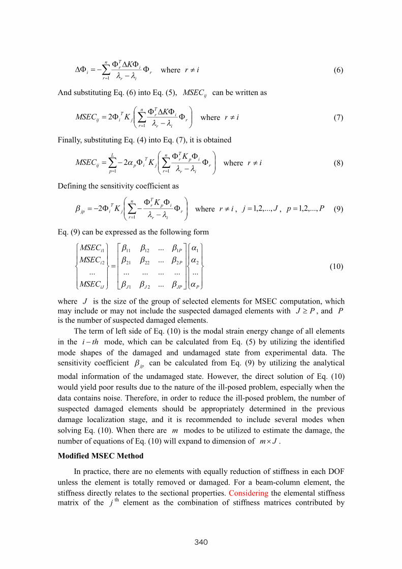
And substituting Eq. (6) into Eq. (5), ijMSEC can be written as

n

r

r

ir

i

T

rj

T

iij

KKMSEC

1

2 where ir (7)

Finally, substituting Eq. (4) into Eq. (7), it is obtained

L

p

n

r

r

ir

ip

T

r

j

T

ipij

KKMSEC

1 1

2 where ir (8)

Defining the sensitivity coefficient as

n

r

r

ir

ip

T

r

j

T

ijp

KK

1

2 where ir , Jj ,...,2,1 , Pp ,...,2,1 (9)

Eq. (9) can be expressed as the following form

PJPJJ

P

P

iJ

i

i

MSEC

MSEC

MSEC

...

...

............

...

...

...

2

1

21

22221

11211

2

1

(10)

where J is the size of the group of selected elements for MSEC computation, which

may include or may not include the suspected damaged elements with PJ , and P

is the number of suspected damaged elements.

The term of left side of Eq. (10) is the modal strain energy change of all elements

in the thi mode, which can be calculated from Eq. (5) by utilizing the identified

mode shapes of the damaged and undamaged state from experimental data. The

sensitivity coefficient jp can be calculated from Eq. (9) by utilizing the analytical

modal information of the undamaged state. However, the direct solution of Eq. (10)

would yield poor results due to the nature of the ill-posed problem, especially when the

data contains noise. Therefore, in order to reduce the ill-posed problem, the number of

suspected damaged elements should be appropriately determined in the previous

damage localization stage, and it is recommended to include several modes when

solving Eq. (10). When there are m modes to be utilized to estimate the damage, the

number of equations of Eq. (10) will expand to dimension of Jm .

Modified MSEC Method

In practice, there are no elements with equally reduction of stiffness in each DOF

unless the element is totally removed or damaged. For a beam-column element, the

stiffness directly relates to the sectional properties. Considering the elemental stiffness

matrix of the jthelement as the combination of stiffness matrices contributed by

340

different sectional properties, the variation of the stiffness matrix for jthelement can

be expressed as

111122223333 I

j

I

j

I

j

I

j

I

j

I

j

A

j

A

jj KKKKK (11)

where superscript A denotes the one related to the cross sectional area, superscript

33I or 22I denotes the one related to the moment of inertia about the local 3rdaxis or

2ndaxis, respectively, and superscript 11I denotes the one related to the torsional

constant. Therefore, the first order modal strain energy change of jthelement in the i

th

mode due to the variation of mode shape and different sectional properties are expressed

as

i

I

j

T

i

i

I

j

T

i

i

I

j

T

i

i

A

j

T

i

ij

K

K

K

K

MSEC

11

22

33

2 (12)

And the sensitivity coefficient is modified as

11112211331111

11222222332222

11332233333333

112233

II

jp

II

jp

II

jp

AI

jp

II

jp

II

jp

II

jp

AI

jp

II

jp

II

jp

II

jp

AI

jp

AI

jp

AI

jp

AI

jp

AA

jp

jp (13)

in which the typical component of sensitivity coefficient jp is expressed as

n

r

r

ir

i

I

p

T

rA

j

T

i

AI

jp

KK

1

33

33 2 where ir (14)

where the combination of superscript A or 33I can be replaced by any other

combination of A , 33I , 22I , and J .

Because the natural frequencies are determined much more accurately than the

mode shapes, and the incoroporation of the change of system natural frequency and

MSEC may also reduce the posibiliy of ill-posed sensitivity matrix, and the sensitivity

equations of the variation of natural frequencies is:

i

ij

T

i

ii

d

iif

Kfff

2

0

8(15)

are added to Eq. (10), where d

if is the measured natural frequency of the ithmode of

the damage system, and 0

if is the measured intact natural frequency of the ithmode,

hence Eq. (10) turns into

341

P

JPJJ

P

P

i

iJ

T

i

i

i

T

i

i

i

T

i

iJ

i

i

i

f

K

f

K

f

K

MSEC

MSEC

MSEC

f

...

...

............

...

...

8...

88

...

2

1

21

22221

11211

22

2

2

1

2

1

(16)

Finally, Eq. (12), Eq. (13) and Eq. (14) are substituted into Eq. (16) to solve for the

stiffness reduction factor of different sectional property of each element.

Dynamic Modal Expansion

The dynamic expansion is a well known reduction and expansion method based on

the undamped dynamic equation of the system. [10] The unmeasured DOFs of the

current structure state can be obtained by expanding the measured DOFs of the structure

based on the following equation

msmissis MKMK )()(212

(11)

where subscript m relates to master DOFs (measured DOFs), and subscript s relates

to slave DOFs (un-measured DOFs). The mode shape with full DOFs can be obtained

by expanding the incomplete measured mode shape using this dynamic modal

expansion algorithm.

Modified Iteration Process

Because the relation between the MSEC and the damage reduction factor j is

nonlinear when enough damage has occurred to cause the shift of the system natural

frequency and stiffness, iteration process is required to obtain more accurate assessment

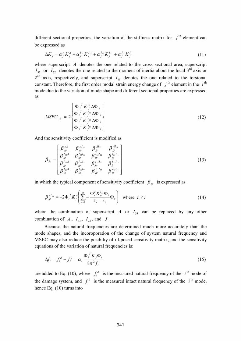
of damage severity. Ricles and Kosmatka had proposed an iteration process coping with

the nonlinearity [11] as illustrated in Fig. 1(a), where the superscripts 0, 1, and 2 refer to

the linearization points during updating, and 0 and d are arrays containing modal

parameters including natural frequency and MSE of the intact and damaged structure,

respectively. The difference between 0 and d is actually the left side of Eq.(16).

In the ithstep, the stiffness reduction factor array i is calculated by Eq. (16) which

considering the current structural state rather than the intact structural state. Finally, the

accumulated stiffness reduction factor array is obtained by summing all the stiffness

reduction factor array i .

The target of the iteration process is d , which is assumed fixed during the

iteration. The natural frequency in d is directly the measured one in the damaged

state. However, the other target, MSE in the damaged state, is obtained by dynamic

expanding the measured mode shape in the damaged state according to the stiffness

matrix. In the original iteration process, the intact stiffness matrix is utilized and

remains unchanged during the iteration. We propose to use the stiffness matrix updated

based on the results of the previous step in each iteration step to expand the measured

342

mode shape, hence the updated target MSE is utilized during the iteration process. The

modified iteration process is demonstrated in Fig. 1(b).

d

0

0

1

1

1

11

2

2 0

Fixed

Target

Structural

Parameter

= Updated Linearization Point

0d

0

0

1

1

2

2 0

1d

2d

Fig. 1 Iteration process (a) original; (b) modified

Convergence Criterion

In practice, the true damage state is unknown. Therefore, certain criterion is

required to evaluate the results obtained by the modified MSEC method. Actually, both

the natural frequency, mode shape, and stiffness matrix must satisfy the equation of

motion, i.e. 0)( 2

iiMK , but the residual is not a scalar. In this study, we use the

measured damaged natural frequency as the target, and define the target ratio (TR) as

the convergence criterion

d

i

o

i

d

i

j

ii

ff

ffTR (11)

where j

if is the calculated natural frequency of the ithmode in the j

thiteration. The

advantage of using natural frequency based convergence criterion is that the natural

frequency is measured directly and also reliable. This simple convergence criterion

provides a roughly idea about the reliability of the results.

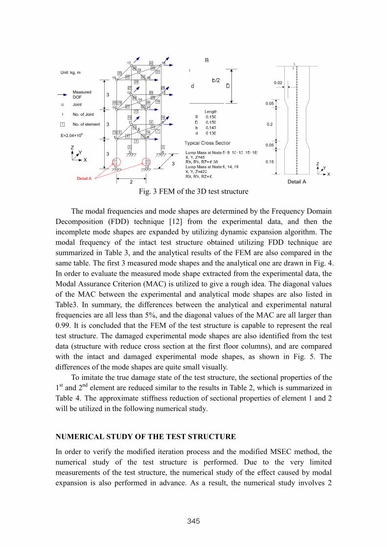
EXPERIMENTAL SETUP AND FEM OF THE TEST STRUCTURE

Experimental Setup of the Test Structure

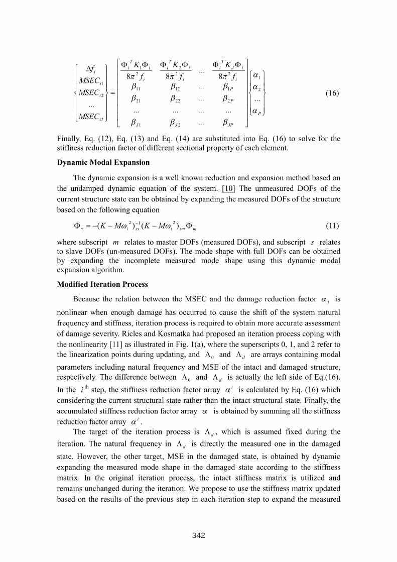
The modified MSEC procedure is evaluated using modal data extracted from a shaking

table test of a 3D structure, which is a full-scale 1-bay × 1-bay × 3-story steel frame

structure (Fig. 2). The dimension of the test structure is 2m, 3m and 9m in X, Y and Z

direction, respectively. The dead load is simulated by lead-block units fixed on the steel

plate of each floor, results in the total mass of each floor of the test structure is 5,943 kg.

To imitate the damage state which is like the plastic hinge of the column, the flanges of

343

the bottom of the first story column are sliced with 2cm wide and 20cm long for both

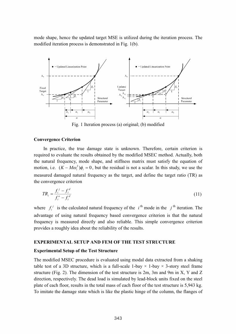
sides. According to the numerical study of the entire damaged column of the first floor

by SAP2000 software, the force need to achieve 1 unit deformation in each DOF on the

top of the designated-damaged column (i.e. the point No. 5 and 6 in Fig. 3) is deducted

to different extent which is summarized in Table 2.

Fig. 2 Photo of the 3-D experimental test structure

The test structure was subjected to El Centro earthquakes and random vibration

simulated by the shaking table in National Center of Research on Earthquake

Engineering (NCREE), Taiwan, R.O.C.. Unilateral, bilateral, and torsional excitation

from shaking table test with amplitude 100 gal are conducted both before and after the

s during the

tests are measured only at point 6, 8, 11, 13, 16, and 18 in the X direction and point 7, 8,

12, 13, 17, and 18 in the Y direction.

To give an outline of the limited number of measured DOFs of the test structure in

this study, the Coefficient of Measurement Density (CMD) is defined as (measured

number of DOFs)/((number of elements)×(number of DOFs per node)). The CMD of

the test structure is (12)/(36×6)=1/18, on the other hand, the CMD of the experimental

case study of the original paper [6] is (16)/(18×3)=8/27, which is more than 5 times of

the CMD of the test structure. Accordingly, the hardship for damage detection of this

test structure can be anticipated.

FEM of Test Structure

The FEM of test structure is simplified and condensed into 36 beam-column

elements. Each of the point has 6 DOFs, therefore there are 90 DOFs totally. The axial

stiffness of the elements No. 9~12, 21~24, 33~36 are magnified to simulate the stiffness

contribution of the steel plate and lead block units. The distribution of the mass of each

joint in each floor is manually adjusted to fit the experimental modal results. The details

of the geometrical and physical information of the test structure are shown in Fig.3.

X

Global

Coordinate

Reduced

Quantity

Z -2.5%

X -20.3%

Y -5.5%

RZ -3.1%

RX -6.8%

RY -25.2%

Table 2: Stiffness reduction of each DOF

on the top of the sliced column

344

1 2

3 4

5

6 7

8

9 10

1112

17

18 19

20

21 22

2324

13 14

15 16

29

30 31

32

33 34

3536

25 26

27 28

2

31 2

3 4

5 6

7 8

10 11

12 13

9

14

15 16

17 18

19

1

1

X

YZ

No. of Joint

No. of element

Joint

Detail A

Measured

DOF

3

3

3

Unit: kg, m

E=2.04×106

0.15

0.05

0.2

0.05

0.02

X

YZ

Detail A

Fig. 3 FEM of the 3D test structure

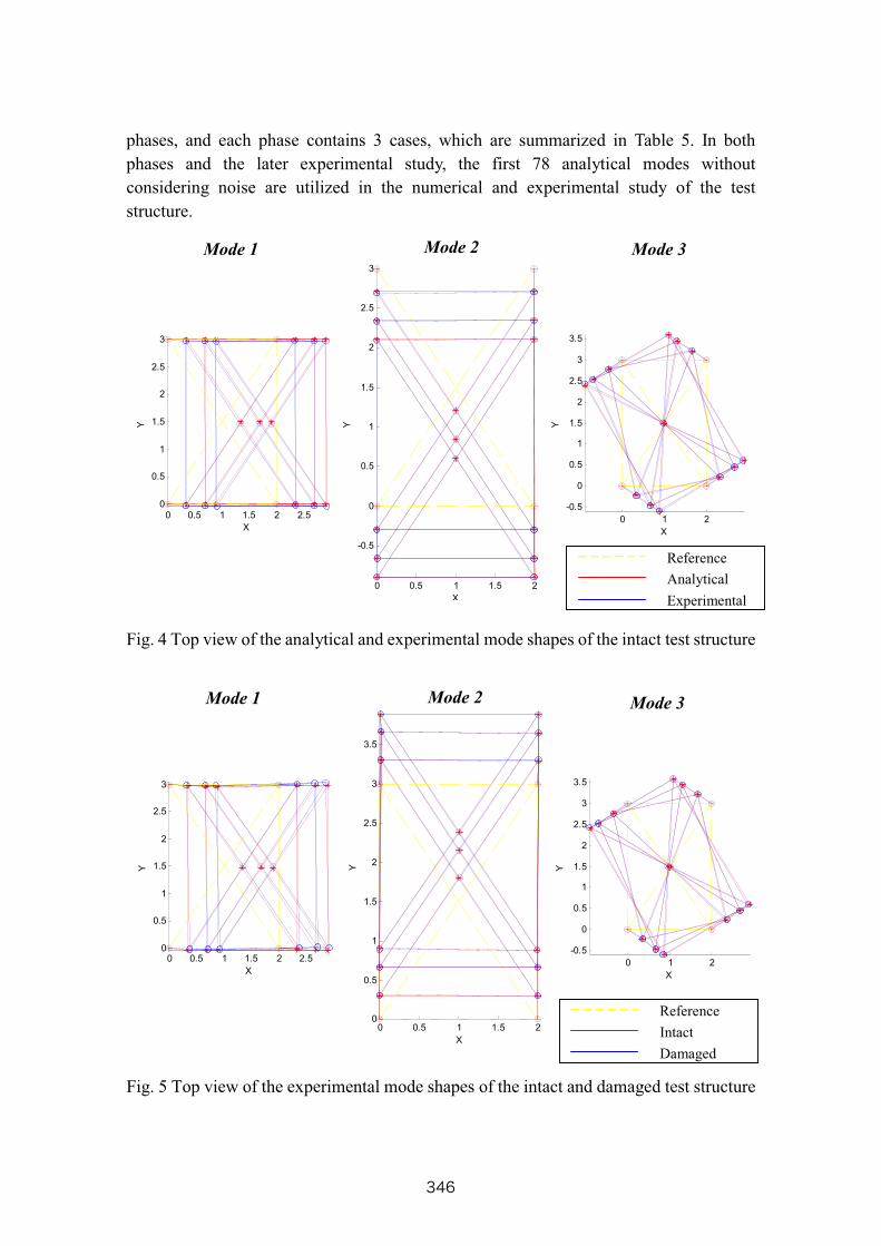
The modal frequencies and mode shapes are determined by the Frequency Domain

Decomposition (FDD) technique [12] from the experimental data, and then the

incomplete mode shapes are expanded by utilizing dynamic expansion algorithm. The

modal frequency of the intact test structure obtained utilizing FDD technique are

summarized in Table 3, and the analytical results of the FEM are also compared in the

same table. The first 3 measured mode shapes and the analytical one are drawn in Fig. 4.

In order to evaluate the measured mode shape extracted from the experimental data, the

Modal Assurance Criterion (MAC) is utilized to give a rough idea. The diagonal values

of the MAC between the experimental and analytical mode shapes are also listed in

Table3. In summary, the differences between the analytical and experimental natural

frequencies are all less than 5%, and the diagonal values of the MAC are all larger than

0.99. It is concluded that the FEM of the test structure is capable to represent the real

test structure. The damaged experimental mode shapes are also identified from the test

data (structure with reduce cross section at the first floor columns), and are compared

with the intact and damaged experimental mode shapes, as shown in Fig. 5. The

differences of the mode shapes are quite small visually.

To imitate the true damage state of the test structure, the sectional properties of the

1stand 2

ndelement are reduced similar to the results in Table 2, which is summarized in

Table 4. The approximate stiffness reduction of sectional properties of element 1 and 2

will be utilized in the following numerical study.

NUMERICAL STUDY OF THE TEST STRUCTURE

In order to verify the modified iteration process and the modified MSEC method, the

numerical study of the test structure is performed. Due to the very limited

measurements of the test structure, the numerical study of the effect caused by modal

expansion is also performed in advance. As a result, the numerical study involves 2

345

phases, and each phase contains 3 cases, which are summarized in Table 5. In both

phases and the later experimental study, the first 78 analytical modes without

considering noise are utilized in the numerical and experimental study of the test

structure.

0 0.5 1 1.5 2 2.50

0.5

1

1.5

2

2.5

3

X

Y

0 0.5 1 1.5 2

-0.5

0

0.5

1

1.5

2

2.5

3

X

Y

0 1 2

-0.5

0

0.5

1

1.5

2

2.5

3

3.5

X

Y

Fig. 4 Top view of the analytical and experimental mode shapes of the intact test structure

0 0.5 1 1.5 2 2.50

0.5

1

1.5

2

2.5

3

X

Y

0 0.5 1 1.5 20

0.5

1

1.5

2

2.5

3

3.5

X

Y

0 1 2

-0.5

0

0.5

1

1.5

2

2.5

3

3.5

X

Y

Fig. 5 Top view of the experimental mode shapes of the intact and damaged test structure

Mode 1 Mode 2 Mode 3

Reference

Analytical

Experimental

Reference

Intact

Damaged

Mode 1 Mode 2 Mode 3

346

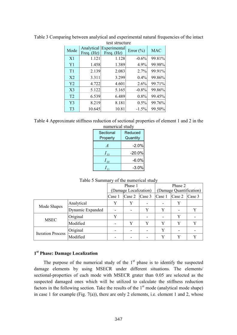
Table 3 Comparing between analytical and experimental natural frequencies of the intact

test structure

ModeAnalyticalFreq. (Hz)

ExperimentalFreq. (Hz)

Error (%) MAC

X1 1.121 1.128 -0.6% 99.81%

Y1 1.458 1.389 4.9% 99.98%

T1 2.139 2.083 2.7% 99.91%

X2 3.311 3.299 0.4% 99.86%

Y2 4.722 4.601 2.6% 99.71%

X3 5.122 5.165 -0.8% 99.86%

T2 6.539 6.489 0.8% 99.45%

Y3 8.219 8.181 0.5% 99.76%

T3 10.645 10.81 -1.5% 99.50%

Table 4 Approximate stiffness reduction of sectional properties of element 1 and 2 in the

numerical study

Sectional

Property

Reduced

Quantity

A -2.0%

33I -20.0%

22I -6.0%

11I -3.0%

Table 5 Summary of the numerical studyPhase 1

(Damage Localization)Phase 2

(Damage Quantification)

Case 1 Case 2 Case 3 Case 1 Case 2 Case 3

Analytical Y Y - - YMode Shapes

Dynamic Expanded - - Y Y - Y

Original Y - - Y -MSEC

Modified - Y Y Y Y Y

Original - - - Y - -Iteration Process

Modified - - - Y Y Y

1stPhase: Damage Localization

The purpose of the numerical study of the 1stphase is to identify the suspected

damage elements by using MSECR under different situations. The elements/

sectional-properties of each mode with MSECR grater than 0.05 are selected as the

suspected damaged ones which will be utilized to calculate the stiffness reduction

factors in the following section. Take the results of the 1stmode (analytical mode shape)

in case 1 for example (Fig. 7(a)), there are only 2 elements, i.e. element 1 and 2, whose

347

MSECR are greater than 0.05. Therefore, only these 2 elements are selected as the

suspected damaged elements and utilized to calculate the stiffness reduction factors for

the 1stmode. The difference between case 1 and case 2 is the calculation of MSECR.

The other example is the results obtained by the 1stmode in case 3 (Fig. 7(c)). There are

3 sectional-properties whose MSECR exceed the limit, i.e. 33I of the element 1, 33I

of the element 2, and the 22I of the element 5.

In order to simplify the comparison of the results obtained by different methods in

the numerical study of the 2ndphase, the suspected damaged elements/sectional

-properties are selected considering the same mode numbers, rather than the individual

mode. For example, the 1st, 4

thand 6

thmode are the 1

st, 2

ndand 3

rdmode of the

X-direction, respectively, and the average MSECR of these 3 modes is considered to

locate the suspected damage elements/sectional-properties. Similarly, the 2nd, 5th, and 8

th

modes are considered together, and the 3rd, 7th, and 9

thmodes are considered together.

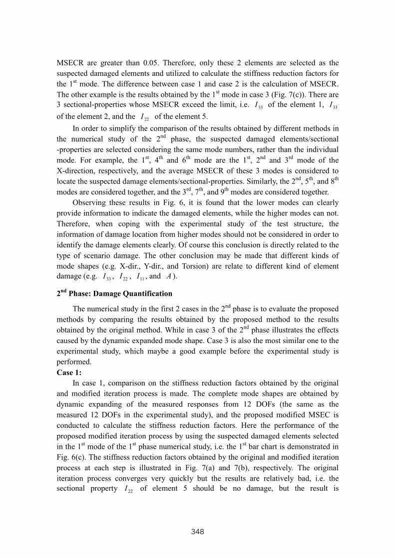
Observing these results in Fig. 6, it is found that the lower modes can clearly

provide information to indicate the damaged elements, while the higher modes can not.

Therefore, when coping with the experimental study of the test structure, the

information of damage location from higher modes should not be considered in order to

identify the damage elements clearly. Of course this conclusion is directly related to the

type of scenario damage. The other conclusion may be made that different kinds of

mode shapes (e.g. X-dir., Y-dir., and Torsion) are relate to different kind of element

damage (e.g. 33I , 22I , 11I , and A ).

2ndPhase: Damage Quantification

The numerical study in the first 2 cases in the 2ndphase is to evaluate the proposed

methods by comparing the results obtained by the proposed method to the results

obtained by the original method. While in case 3 of the 2ndphase illustrates the effects

caused by the dynamic expanded mode shape. Case 3 is also the most similar one to the

experimental study, which maybe a good example before the experimental study is

performed.

Case 1:

In case 1, comparison on the stiffness reduction factors obtained by the original

and modified iteration process is made. The complete mode shapes are obtained by

dynamic expanding of the measured responses from 12 DOFs (the same as the

measured 12 DOFs in the experimental study), and the proposed modified MSEC is

conducted to calculate the stiffness reduction factors. Here the performance of the

proposed modified iteration process by using the suspected damaged elements selected

in the 1stmode of the 1

stphase numerical study, i.e. the 1

stbar chart is demonstrated in

Fig. 6(c). The stiffness reduction factors obtained by the original and modified iteration

process at each step is illustrated in Fig. 7(a) and 7(b), respectively. The original

iteration process converges very quickly but the results are relatively bad, i.e. the

sectional property 22I of element 5 should be no damage, but the result is

348

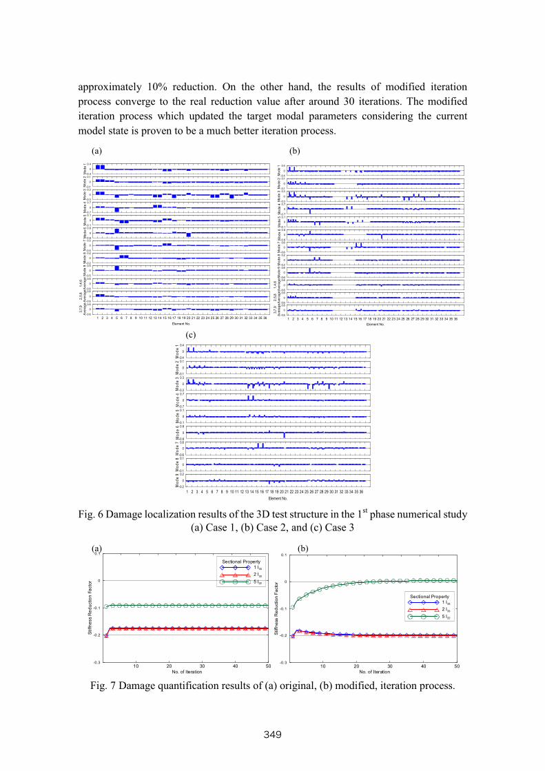
approximately 10% reduction. On the other hand, the results of modified iteration

process converge to the real reduction value after around 30 iterations. The modified

iteration process which updated the target modal parameters considering the current

model state is proven to be a much better iteration process.

-0.4

0

0.4

Mode1

-0.1

0

0.1

Mode2

-0.3

0

0.3

Mode3

-0.7

0

0.7

Mode4

-0.1

0

0.1

Mode5

-0.6

0

0.6

Mode6

Element No.

-0.5

0

0.5

Mode7

-0.2

0

0.2

Mode8

-0.5

0

0.5

Mode9

-0.6

0

0.6

1,4,6

Average

-0.6

0

0.6

2,5,8

Average

1 2 3 4 5 6 7 8 9 10 11 12 13 14 15 16 17 18 19 20 21 22 23 24 25 26 27 28 29 30 31 32 33 34 35 36-0.6

0

0.6

3,7,9

Average

-0.4

0

0.4

Mode1

-0.1

0

0.1

Mode2

-0.3

0

0.3

Mode3

-0.7

0

0.7

Mode4

-0.1

0

0.1

Mode5

-0.6

0

0.6

Mode6

Element No.

-0.6

0

0.6

Mode7

-0.2

0

0.2

Mode8

-0.6

0

0.6

Mode9

-0.6

0

0.6

1,4,6

Average

-0.6

0

0.6

2,5,8

Average

1 2 3 4 5 6 7 8 9 10 11 12 13 14 15 16 17 18 19 20 21 22 23 24 25 26 27 28 29 30 31 32 33 34 35 36

-0.6

0

0.6

3,7,9

Average

-0.4

0

0.4

Mode1

-0.1

0

0.1

Mode2

-0.3

0

0.3

Mode3

-0.7

0

0.7

Mode4

-0.1

0

0.1

Mode5

-0.6

0

0.6

Mode6

Element No.

-0.6

0

0.6

Mode7

-0.1

0

0.1

Mode8

1 2 3 4 5 6 7 8 9 10 11 12 13 14 15 16 17 18 19 20 21 22 23 24 25 26 27 28 29 30 31 32 33 34 35 36

-0.2

0

0.2

Mode9

Fig. 6 Damage localization results of the 3D test structure in the 1stphase numerical study

(a) Case 1, (b) Case 2, and (c) Case 3

10 20 30 40 50-0.3

-0.2

-0.1

0

0.1

StiffnessReductionFactor

Sectional Property

1 I33

2 I33

5 I22

No. of Iteration

10 20 30 40 50-0.3

-0.2

-0.1

0

0.1

StiffnessReductionFactor

Sectional Property

1 I33

2 I33

5 I22

No. of Iteration

Fig. 7 Damage quantification results of (a) original, (b) modified, iteration process.

(a) (b)

(c)

(a) (b)

349

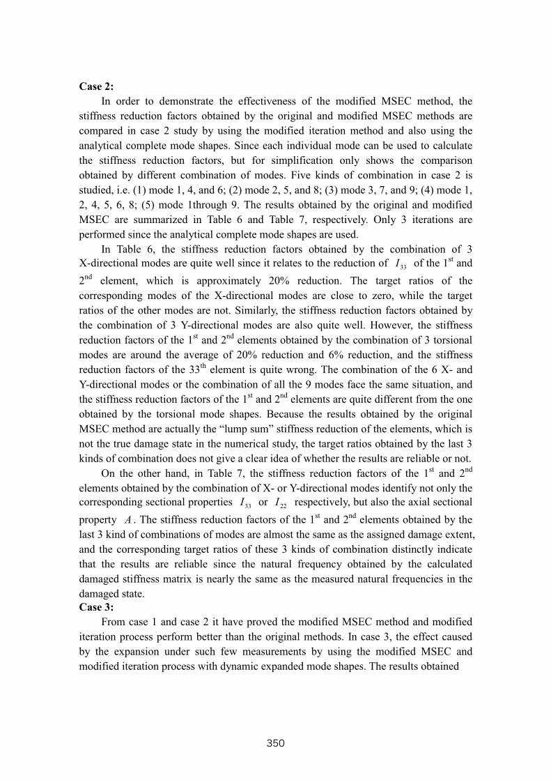
Case 2:

In order to demonstrate the effectiveness of the modified MSEC method, the

stiffness reduction factors obtained by the original and modified MSEC methods are

compared in case 2 study by using the modified iteration method and also using the

analytical complete mode shapes. Since each individual mode can be used to calculate

the stiffness reduction factors, but for simplification only shows the comparison

obtained by different combination of modes. Five kinds of combination in case 2 is

studied, i.e. (1) mode 1, 4, and 6; (2) mode 2, 5, and 8; (3) mode 3, 7, and 9; (4) mode 1,

2, 4, 5, 6, 8; (5) mode 1through 9. The results obtained by the original and modified

MSEC are summarized in Table 6 and Table 7, respectively. Only 3 iterations are

performed since the analytical complete mode shapes are used.

In Table 6, the stiffness reduction factors obtained by the combination of 3

X-directional modes are quite well since it relates to the reduction of 33I of the 1stand

2ndelement, which is approximately 20% reduction. The target ratios of the

corresponding modes of the X-directional modes are close to zero, while the target

ratios of the other modes are not. Similarly, the stiffness reduction factors obtained by

the combination of 3 Y-directional modes are also quite well. However, the stiffness

reduction factors of the 1stand 2

ndelements obtained by the combination of 3 torsional

modes are around the average of 20% reduction and 6% reduction, and the stiffness

reduction factors of the 33thelement is quite wrong. The combination of the 6 X- and

Y-directional modes or the combination of all the 9 modes face the same situation, and

the stiffness reduction factors of the 1stand 2

ndelements are quite different from the one

obtained by the torsional mode shapes. Because the results obtained by the original

which is

not the true damage state in the numerical study, the target ratios obtained by the last 3

kinds of combination does not give a clear idea of whether the results are reliable or not.

On the other hand, in Table 7, the stiffness reduction factors of the 1stand 2

nd

elements obtained by the combination of X- or Y-directional modes identify not only the

corresponding sectional properties 33I or 22I respectively, but also the axial sectional

property A . The stiffness reduction factors of the 1stand 2

ndelements obtained by the

last 3 kind of combinations of modes are almost the same as the assigned damage extent,

and the corresponding target ratios of these 3 kinds of combination distinctly indicate

that the results are reliable since the natural frequency obtained by the calculated

damaged stiffness matrix is nearly the same as the measured natural frequencies in the

damaged state.

Case 3:

From case 1 and case 2 it have proved the modified MSEC method and modified

iteration process perform better than the original methods. In case 3, the effect caused

by the expansion under such few measurements by using the modified MSEC and

modified iteration process with dynamic expanded mode shapes. The results obtained

350

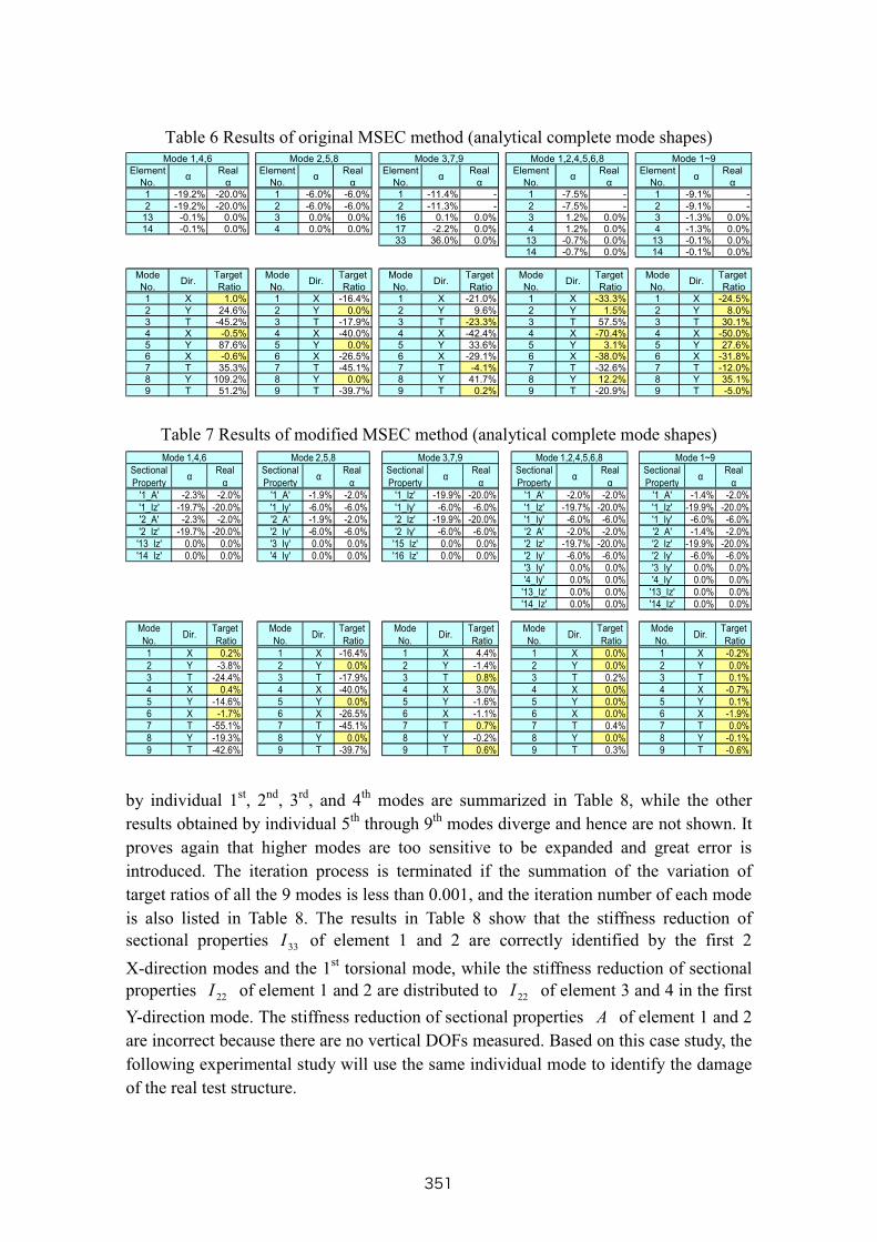
Table 6 Results of original MSEC method (analytical complete mode shapes)

Element

No.

Real Element

No.

Real Element

No.

Real Element

No.

Real Element

No.

Real

1 -19.2% -20.0% 1 -6.0% -6.0% 1 -11.4% - 1 -7.5% - 1 -9.1% -

2 -19.2% -20.0% 2 -6.0% -6.0% 2 -11.3% - 2 -7.5% - 2 -9.1% -13 -0.1% 0.0% 3 0.0% 0.0% 16 0.1% 0.0% 3 1.2% 0.0% 3 -1.3% 0.0%

14 -0.1% 0.0% 4 0.0% 0.0% 17 -2.2% 0.0% 4 1.2% 0.0% 4 -1.3% 0.0%

33 36.0% 0.0% 13 -0.7% 0.0% 13 -0.1% 0.0%

14 -0.7% 0.0% 14 -0.1% 0.0%

Mode

No.Dir.

Target

Ratio

Mode

No.Dir.

Target

Ratio

Mode

No.Dir.

Target

Ratio

Mode

No.Dir.

Target

Ratio

Mode

No.Dir.

Target

Ratio

1 X 1.0% 1 X -16.4% 1 X -21.0% 1 X -33.3% 1 X -24.5%

2 Y 24.6% 2 Y 0.0% 2 Y 9.6% 2 Y 1.5% 2 Y 8.0%

3 T -45.2% 3 T -17.9% 3 T -23.3% 3 T 57.5% 3 T 30.1%

4 X -0.5% 4 X -40.0% 4 X -42.4% 4 X -70.4% 4 X -50.0%

5 Y 87.6% 5 Y 0.0% 5 Y 33.6% 5 Y 3.1% 5 Y 27.6%6 X -0.6% 6 X -26.5% 6 X -29.1% 6 X -38.0% 6 X -31.8%

7 T 35.3% 7 T -45.1% 7 T -4.1% 7 T -32.6% 7 T -12.0%

8 Y 109.2% 8 Y 0.0% 8 Y 41.7% 8 Y 12.2% 8 Y 35.1%

9 T 51.2% 9 T -39.7% 9 T 0.2% 9 T -20.9% 9 T -5.0%

Mode 3,7,9 Mode 1,2,4,5,6,8 Mode 1~9Mode 1,4,6 Mode 2,5,8

Table 7 Results of modified MSEC method (analytical complete mode shapes)

Sectional

Property

Real Sectional

Property

Real Sectional

Property

Real Sectional

Property

Real Sectional

Property

Real

'1_A' -2.3% -2.0% '1_A' -1.9% -2.0% '1_Iz' -19.9% -20.0% '1_A' -2.0% -2.0% '1_A' -1.4% -2.0%

'1_Iz' -19.7% -20.0% '1_Iy' -6.0% -6.0% '1_Iy' -6.0% -6.0% '1_Iz' -19.7% -20.0% '1_Iz' -19.9% -20.0%

'2_A' -2.3% -2.0% '2_A' -1.9% -2.0% '2_Iz' -19.9% -20.0% '1_Iy' -6.0% -6.0% '1_Iy' -6.0% -6.0%

'2_Iz' -19.7% -20.0% '2_Iy' -6.0% -6.0% '2_Iy' -6.0% -6.0% '2_A' -2.0% -2.0% '2_A' -1.4% -2.0%

'13_Iz' 0.0% 0.0% '3_Iy' 0.0% 0.0% '15_Iz' 0.0% 0.0% '2_Iz' -19.7% -20.0% '2_Iz' -19.9% -20.0%

'14_Iz' 0.0% 0.0% '4_Iy' 0.0% 0.0% '16_Iz' 0.0% 0.0% '2_Iy' -6.0% -6.0% '2_Iy' -6.0% -6.0%

'3_Iy' 0.0% 0.0% '3_Iy' 0.0% 0.0%

'4_Iy' 0.0% 0.0% '4_Iy' 0.0% 0.0%

'13_Iz' 0.0% 0.0% '13_Iz' 0.0% 0.0%

'14_Iz' 0.0% 0.0% '14_Iz' 0.0% 0.0%

Mode

No.Dir.

Target

Ratio

Mode

No.Dir.

Target

Ratio

Mode

No.Dir.

Target

Ratio

Mode

No.Dir.

Target

Ratio

Mode

No.Dir.

Target

Ratio

1 X 0.2% 1 X -16.4% 1 X 4.4% 1 X 0.0% 1 X -0.2%

2 Y -3.8% 2 Y 0.0% 2 Y -1.4% 2 Y 0.0% 2 Y 0.0%

3 T -24.4% 3 T -17.9% 3 T 0.8% 3 T 0.2% 3 T 0.1%

4 X 0.4% 4 X -40.0% 4 X 3.0% 4 X 0.0% 4 X -0.7%

5 Y -14.6% 5 Y 0.0% 5 Y -1.6% 5 Y 0.0% 5 Y 0.1%

6 X -1.7% 6 X -26.5% 6 X -1.1% 6 X 0.0% 6 X -1.9%

7 T -55.1% 7 T -45.1% 7 T 0.7% 7 T 0.4% 7 T 0.0%

8 Y -19.3% 8 Y 0.0% 8 Y -0.2% 8 Y 0.0% 8 Y -0.1%

9 T -42.6% 9 T -39.7% 9 T 0.6% 9 T 0.3% 9 T -0.6%

Mode 3,7,9 Mode 1,2,4,5,6,8 Mode 1~9Mode 1,4,6 Mode 2,5,8

by individual 1st, 2

nd, 3

rd, and 4

thmodes are summarized in Table 8, while the other

results obtained by individual 5ththrough 9

thmodes diverge and hence are not shown. It

proves again that higher modes are too sensitive to be expanded and great error is

introduced. The iteration process is terminated if the summation of the variation of

target ratios of all the 9 modes is less than 0.001, and the iteration number of each mode

is also listed in Table 8. The results in Table 8 show that the stiffness reduction of

sectional properties 33I of element 1 and 2 are correctly identified by the first 2

X-direction modes and the 1sttorsional mode, while the stiffness reduction of sectional

properties 22I of element 1 and 2 are distributed to 22I of element 3 and 4 in the first

Y-direction mode. The stiffness reduction of sectional properties A of element 1 and 2

are incorrect because there are no vertical DOFs measured. Based on this case study, the

following experimental study will use the same individual mode to identify the damage

of the real test structure.

351

Table 8 Results of modified MSEC method (dynamic expanded mode shapes)

Sectional

Property

Real Sectional

Property

Real Sectional

Property

Real Sectional

Property

Real

'1_Iz' -19.9% -2.0% '1_Iy' -3.0% -6.0% '1_Iz' -20.5% -20.0% '1_A' 20.5% -2.0%

'2_Iz' -20.1% -20.0% '2_Iy' -3.0% -6.0% '1_Iy' -3.0% -6.0% '1_Iz' -18.5% -20.0%

'5_Iy' 0.2% -2.0% '3_Iy' -3.0% 0.0% '2_Iz' -20.7% -20.0% '2_A' 20.5% -2.0%

'4_Iy' -3.0% 0.0% '2_Iy' -3.1% -6.0% '2_Iz' -19.1% -20.0%

'6_Iy' -0.1% 0.0% '3_Iz' -2.9% 0.0% '13_Iz' 3.7% 0.0%

'7_Iy' -0.1% 0.0% '3_Iy' -2.8% 0.0% '14_Iz' 2.4% 0.0%

'4_Iz' 0.0% 0.0% '15_Iz' 1.9% 0.0%

'4_Iy' 0.1% 0.0% '16_Iz' 2.0% 0.0%

'5_Iy' 0.0% 0.0% '17_Iy' 0.5% 0.0%

'6_Iy' -0.3% 0.0%

'7_Iy' -0.4% 0.0%

'8_Iy' 3.2% 0.0%

Mode

No.Dir.

Target

Ratio

Mode

No.Dir.

Target

Ratio

Mode

No.Dir.

Target

Ratio

Mode

No.Dir.

Target

Ratio

1 X -0.2% 1 X -16.4% 1 X 115.5% 1 X -2.2%

2 Y -3.9% 2 Y 0.1% 2 Y -62.5% 2 Y -2.9%

3 T -68.8% 3 T -17.9% 3 T 0.0% 3 T 161.0%

4 X -0.6% 4 X -40.0% 4 X 61.0% 4 X 0.0%

5 Y -14.6% 5 Y -0.5% 5 Y -27.2% 5 Y -13.8%

6 X -1.2% 6 X -26.5% 6 X -925.2% 6 X -0.6%

7 T -48.2% 7 T -42.7% 7 T 70.3% 7 T -88.8%

8 Y -19.3% 8 Y -0.6% 8 Y 136.8% 8 Y -19.3%

9 T -44.6% 9 T -36.3% 9 T -245.8% 9 T -17.6%

Mode 1 (ITE=30) Mode 2 (ITE=21) Mode 3 (ITE=6) Mode 4 (ITE=12)

EXPERIMENTAL DAMAGE DETECTION

Damage Localization

The measured mode shapes of the intact and damaged structure are utilized for

damage localization. Due to the noise and other disturbance in the test, the threshold of

MSE MSEC is chosen as 0.3 in the experimental study. Similar to the results of

numerical study (Fig. 6(c)), the damage locations can be successfully identified by only

the first 3 modes. It should be noted that the MSECR value of the 4thmode can not

identify the damage locations, which implies the damage quantification obtained by the

4thmode may not be as good as the numerical study. The sectional properties with

MSECR greater than 0.05 of the first 4 individual mode are chosen to calculate the

stiffness reduction factors.

Damage Quantification

The measured mode shapes and natural frequencies of the intact and damaged structure

are utilized for damage quantification. Based on the results of numerical study, the

stiffness reduction factors obtained using the first 4 individual modes are listed in Table

9. Because the iteration process fails to converge for these 4 modes, only the results

obtained at the first iteration are shown. From the results, it seems that the stiffness

reduction of sectional properties 33I of element 1 and 2 are properly

identified by the first 2 X-direction modes and the 1sttorsional mode, and the target

ratios of the corresponding modes are nearly zero. However, the other sectional

properties of other elements are identified as some moderate amount of stiffness

352

and noise effect et al. The combination of any modes does not improve the results of

damage quantification and hence not shown here.

As discussed previously, the number of measured DOFs is relative sparse which

leads to great error caused by expansion of incomplete mode shapes. The modeling

error is also a tough question of the model based identification method. Although the

MAC value and cross-orthogonality check (COR, which is not shown in this paper) of

the measured and analytical mode shapes are quite excellent, it seems that the modeling

error still introduce great error to the modified MSEC method. Further study is needed

to identify the effect of modeling error. In this study, certain amount of noise should

introduce moderate level of errors for damage quantification since the MSEC method

has been proved noise sensitive in damage quantification [6].

-0.4

0

0.4

Mode1

-0.1

0

0.1

Mode2

-0.3

0

0.3

Mode3

-0.7

0

0.7

Mode4

-0.2

0

0.2

Mode5

-0.6

0

0.6

Mode6

Element No.

-0.6

0

0.6

Mode7

-0.3

0

0.3

Mode8

1 2 3 4 5 6 7 8 9 10 11 12 13 14 15 16 17 18 19 20 21 22 23 24 25 26 27 28 29 30 31 32 33 34 35 36

-0.4

0

0.4

Mode9

Fig. 8 Experimental damage localization results of the test structure

CONCLUSIONS

The modified MSEC method to detect structural damage and corresponding

modified iteration process are proposed in this paper. Numerical results using a 3-D

frame structure clearly illustrate the following:

(1) The reduction of sectional properties rather than lump stiffness of elements can

be identified by the proposed modified MSEC method, hence the torsional

modes and the combination of different kind of modes become capable to

identify the correct damage extent.

353

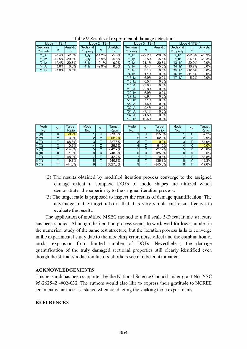
Table 9 Results of experimental damage detection

Sectional

Property

Analytic Sectional

Property

Analytic Sectional

Property

Analytic Sectional

Property

Analytic

'1_A' -2.4% -2.5% '1_Iy' -14.2% -5.5% '1_Iz' -22.2% -20.3% '1_Iz' -22.3% -20.3%

'1_Iz' -16.5% -20.3% '2_Iy' -5.9% -5.5% '1_Iy' 3.5% -5.5% '2_Iz' -24.1% -20.3%

'2_Iz' -17.4% -20.3% '3_Iy' 0.1% 0.0% '2_Iz' -21.1% -20.3% '13_Iz' 20.0% 0.0%

'4_A' 0.6% 0.0% '4_Iy' -9.9% 0.0% '2_Iy' 4.4% -5.5% '14_Iz' 16.7% 0.0%

'5_Iy' -8.8% 0.0% '3_Iy' 0.1% 0.0% '15_Iz' -12.5% 0.0%

'4_Iy' 1.1% 0.0% '16_Iz' -11.1% 0.0%

'15_Iz' 6.9% 0.0% '17_Iy' 5.2% 0.0%

'16_Iz' 6.5% 0.0%

'18_A' -2.0% 0.0%

'19_A' -2.8% 0.0%

'20_Iy' 6.9% 0.0%

'27_Iz' 6.9% 0.0%

'28_Iz' 7.1% 0.0%

'29_A' -4.5% 0.0%

'30_A' -9.4% 0.0%

'31_A' -7.1% 0.0%

'32_A' -1.5% 0.0%

'32_Iy' 12.5% 0.0%

Mode

No.Dir.

Target

Ratio

Mode

No.Dir.

Target

Ratio

Mode

No.Dir.

Target

Ratio

Mode

No.Dir.

Target

Ratio

1 (X) X -0.2% 1 X -73.8% 1 X 115.5% 1 X -2.2%

2 (Y) Y -3.9% 2 Y -362.2% 2 Y -62.5% 2 Y -2.9%

3 (T) T -68.8% 3 T -327.6% 3 T 0.0% 3 T 161.0%

4 (X) X -0.6% 4 X -29.6% 4 X 61.0% 4 X 0.0%

5 (Y) Y -14.6% 5 Y -342.7% 5 Y -27.2% 5 Y -13.8%

6 (X) X -1.2% 6 X 748.5% 6 X -925.2% 6 X -0.6%

7 (T) T -48.2% 7 T -142.2% 7 T 70.3% 7 T -88.8%

8 (Y) Y -19.3% 8 Y 540.7% 8 Y 136.8% 8 Y -19.3%

9 (T) T -44.6% 9 T 6527.3% 9 T -245.8% 9 T -17.6%

Mode 1 (ITE=1) Mode 2 (ITE=1) Mode 3 (ITE=1) Mode 4 (ITE=1)

(2) The results obtained by modified iteration process converge to the assigned

damage extent if complete DOFs of mode shapes are utilized which

demonstrates the superiority to the original iteration process.

(3) The target ratio is proposed to inspect the results of damage quantification. The

advantage of the target ratio is that it is very simple and also effective to

evaluate the results.

The application of modified MSEC method to a full scale 3-D real frame structure

has been studied. Although the iteration process seems to work well for lower modes in

the numerical study of the same test structure, but the iteration process fails to converge

in the experimental study due to the modeling error, noise effect and the combination of

modal expansion from limited number of DOFs. Nevertheless, the damage

quantification of the truly damaged sectional properties still clearly identified even

though the stiffness reduction factors of others seem to be contaminated.

ACKNOWLEDGEMENTS

This research has been supported by the National Science Council under grant No. NSC

95-2625 Z -002-032. The authors would also like to express their gratitude to NCREE

technicians for their assistance when conducting the shaking table experiments.

REFERENCES

354

1.

health monitoring of structure and mechanical systems from changes in their vibration characteristics:

Research Rep. No. LA-13070-MS, ESA-EA, Los Alamos National Laboratory,

Los Alamos, N.M.

2.

1057.

3.

699.

4. ion in structures without base-line modal

1649.

5.

844.

6. Shi, Z

1223.

7. al

529.

8. -D Frame Structure Using

XXIV, St. Louis, Missouri, USA, 2006.

9. Thomas R. S., Charles J. C. Joanne L. W. Howard M. A. (1988 Comparison of Several Methods for

Calculating Vibration Mode Shape Derivatives AIAA J., Vol. 26, no. 12, 1506 1511.

10. Kidder, R., Reduction of Structural Frequency Equations , AIAA Journal, Vol. 11, No. 6, 1973.

11. Ricles, J. M., and Kosmatks, J. B. (1992) structures using vibratory

2316.

355