Daily Mean Sea Level Pressure Reconstructions for the ...

Daily Mean Sea Level Pressure Reconstructions for the European–North AtlanticRegion for the Period 1850–2003

T. J. ANSELL,a P. D. JONES,b R. J. ALLAN,a D. LISTER,b D. E. PARKER,a M. BRUNET,c A. MOBERG,d

J. JACOBEIT,e P. BROHAN,a N. A. RAYNER,a E. AGUILAR,c H. ALEXANDERSSON,f M. BARRIENDOS,g

T. BRANDSMA,h N. J. COX,i P. M. DELLA-MARTA,j A. DREBS,k D. FOUNDA,l F. GERSTENGARBE,m

K. HICKEY,n T. JÓNSSON,o J. LUTERBACHER,p Ø. NORDLI,q H. OESTERLE,m M. PETRAKIS,l A. PHILIPP,e

M. J. RODWELL,r O. SALADIE,c J. SIGRO,c V. SLONOSKY,s L. SRNEC,t V. SWAIL,u A. M. GARCÍA-SUÁREZ,v

H. TUOMENVIRTA,k X. WANG,u H. WANNER,p P. WERNER,m D. WHEELER,w AND E. XOPLAKIp

a Hadley Centre, Met Office, Exeter, United Kingdomb CRU, University of East Anglia, Norwich, United Kingdom

c Universitat Rovira i Virgili, Tarragona, Spaind Stockholm University, Stockholm, Sweden

e University of Augsburg, Augsburg, Germanyf Swedish Meteorological and Hydrological Institute, Norrköping, Sweden

g University of Barcelona, Barcelona, Spainh KNMI, De Bilt, Netherlands

i Durham University, Durham, United Kingdomj University of Bern, Bern, Switzerland

k Finnish Meteorological Institute, Helsinki, Finlandl National Observatory of Athens, Athens, Greece

m Potsdam Institute for Climate Impact Research, Potsdam, Germanyn National University of Ireland, Galway, Galway, Ireland

o Icelandic Meteorological Office, Reykjavik, Icelandp University of Bern, and NCCR Climate, Bern, Switzerland

q The Norwegian Meteorological Institute, Oslo, Norwayr ECMWF, Reading, United Kingdom

s McGill University, Montreal, Quebec, Canadat Meteorological and Hydrological Service, Zagreb, Croatia

u Environment Canada, Ontario, Canadav Armagh Observatory, Armagh, Ireland

w University of Sunderland, Sunderland, United Kingdom

(Manuscript received 5 May 2005, in final form 13 October 2005)

ABSTRACT

The development of a daily historical European–North Atlantic mean sea level pressure dataset(EMSLP) for 1850–2003 on a 5° latitude by longitude grid is described. This product was produced using86 continental and island stations distributed over the region 25°–70°N, 70°W–50°E blended with marinedata from the International Comprehensive Ocean–Atmosphere Data Set (ICOADS). The EMSLP fieldsfor 1850–80 are based purely on the land station data and ship observations. From 1881, the blended landand marine fields are combined with already available daily Northern Hemisphere fields. Complete cov-erage is obtained by employing reduced space optimal interpolation. Squared correlations (r2) indicate thatEMSLP generally captures 80%–90% of daily variability represented in an existing historical mean sea levelpressure product and over 90% in modern 40-yr European Centre for Medium-Range Weather ForecastsRe-Analyses (ERA-40) over most of the region. A lack of sufficient observations over Greenland and theMiddle East, however, has resulted in poorer reconstructions there. Error estimates, produced as part of thereconstruction technique, flag these as regions of low confidence. It is shown that the EMSLP daily fieldsand associated error estimates provide a unique opportunity to examine the circulation patterns associatedwith extreme events across the European–North Atlantic region, such as the 2003 heat wave, in the contextof historical events.

Corresponding author address: Dr. T. J. Ansell, Hadley Centre, Met Office, Fitz Roy Road, Exeter, Devon EX1 3PB, United Kingdom.E-mail: [email protected]

15 JUNE 2006 A N S E L L E T A L . 2717

© 2006 American Meteorological Society

JCLI3775

1. Introduction

The European Community (EC)-funded Europeanand North Atlantic Daily to Multidecadal ClimateVariability Project (EMULATE) began in November2002. An initial aim of EMULATE was to define char-acteristic atmospheric circulation patterns over the Eu-ropean and North Atlantic region. Changes in meanamplitudes, variability, persistence, and transition re-gimes of these dominant patterns over a 154-yr periodwould then be assessed with both traditional and newstatistical techniques. These variations and trendswould be related to sea surface temperature (SST) pat-terns over the North Atlantic and worldwide, and tonatural and anthropogenic forcing factors, involvingvarious climate model integrations. A final aim was torelate these trends to extremes in temperature and pre-cipitation over Europe.

Previous studies of this nature have been limited by alack of gridded mean sea level pressure (MSLP) prod-ucts of sufficient length. Central to EMULATE, there-fore, has been the development of daily gridded MSLPfields over Europe and the extratropical North Atlan-tic, extending back to 1850. These fields will enable usto more fully examine whether relationships betweenSST and circulation patterns are stationary, and then tomore reliably assess the relative importance of anthro-pogenic factors. They will also be used to study thedynamic backgrounds of extreme events and circulationextremes over a well-extended period.

Here we present the development of this griddeddaily MSLP product on a 5° latitude by longitude gridover the region 25°–70°N, 70°W–50°E (hereafter re-ferred to as the EMULATE region). Daily griddedMSLP fields since 1881 for the Northern Hemispherenorth of 15°N are already available (Jackson 1986,hereafter referred to as J86), but are only reliable overwestern and central Europe (e.g., Germany, Austria,Switzerland, and northern Italy). These fields are im-proved and extended, using the long station–based Eu-ropean pressure series from earlier EC projects andrecently digitized long station records, particularly overEurope and Russia. Over the ocean we take advantageof the recently released International ComprehensiveOcean–Atmosphere Data Set (ICOADS; Worley et al.2005; Diaz et al. 2002), using all available observationsover the 24-h period. By blending these sources we areable to produce daily fields from 1850.

The biggest challenge to this work has been the lackof daily observations, particularly before 1881. Duringthis period, observations are available over only 15% ofthe EMULATE region. Despite the inclusion of therecently digitized U.S. Maury collection (before 1863;

Worley et al. 2005), the marine observations are con-strained to the major shipping routes of the time, pre-dominantly between northwest Europe and the Ameri-cas and from northwest Europe to around the Cape ofGood Hope. Similarly, in remote terrestrial regionssuch as central Greenland and northern Africa, no sta-tion data are available. In these areas, our fields arebased purely on reconstruction. Because of this, it isimportant to be able to constrain analyses in these re-gions of low confidence, and accordingly, our Europe-an–North Atlantic mean sea level pressure dataset(EMSLP) is available with error estimates to guide theresearcher.

Quality control and gridding issues, central to thiswork, are described in sections 2 and 3, including theuse of interpolation techniques to obtain spatially com-plete fields. In section 4, we compare EMSLP to exist-ing analyses and examine its ability to resolve extremeevents. In addition to improving the understanding ofrecent events [such as the 2003 summer heat wave inwestern Europe, the autumn 2000 floods in the UnitedKingdom (U.K.), and the European floods in Germany,Austria, and the Czech Republic in 2002 (Danube andElbe rivers)], we expect that this product will be a valu-able aid in the further understanding of historicalextreme events dating back to the mid-nineteenth cen-tury. Conclusions are given in section 5.

2. Data sources and quality control

Our strategy has been to take advantage of a North-ern Hemisphere (north of 15°N) synoptic daily griddedMSLP product available from 1881 to the present (J86),and to improve it while extending the analysis back to1850 with the inclusion of new land station and marinepressure observations. The J86 fields are an extremelyvaluable resource, as they are derived from synopticoperational charts and so implicitly contain many thou-sands of station observations. Because of this, we con-centrated our efforts on collating and digitizing stationdata for the period before 1881. The EMSLP fields for1850–80 are therefore based purely on a blending ofland station data and ship observations; from 1881, theblended land and marine fields are combined with thedaily J86 fields.

Because the number and times of observations perday varies markedly between stations, all the observa-tions (including the marine and J86 fields) are adjustedto represent the 24-hourly mean. Accordingly, theEMSLP daily fields represent the average pressure overthe 24-h period and so are different and indeedsmoother than synoptic and 4� daily reanalysis charts.

2718 J O U R N A L O F C L I M A T E VOLUME 19

a. Terrestrial data sources

The daily continental and island observations weredrawn from a number of sources. Data already in elec-tronic form were obtained for various Italian, Fenno-scandian, and U.K. stations compiled by earlier ECprojects such as Improved understanding of past cli-matic variability from early daily European instrumen-tal sources (IMPROVE; Camuffo and Jones 2002 andreferences therein) and Waves and Storms in the NorthAtlantic (WASA; Schmith et al. 1997), and for the citiesof Montreal, Canada (Slonosky 2003); Gibraltar,United Kingdom; De Bilt, Netherlands; Paris, France;Palermo, Italy; and Galway, Ireland (Hickey et al.2003), by individual efforts (see the acknowledgments).We were able to obtain updates and additional historicdata for some WASA stations, extending them back to1850 and forward to 2003. Considerable material had tobe digitized, however, from individual hard copyrecords from Russian, British, French, and Spanishdaily weather records (DWRs), held in the U.K. Na-tional Meteorological Archives and Library. Thesewere supplemented by scanned Algerian, French, andU.S. observations on the National Oceanic and Atmo-spheric Administration (NOAA) Library Web site(http://docs.lib.noaa.gov/rescue/data_rescue_home-.html). Old American Bulletin of International Meteo-rological Observations volumes also provided valuablerecords for Nuuk (Godthåb), Greenland, and helpedfill gaps in existing records. Data were also digitizedfrom compilations made under the auspices of the U.K.Board of Trade, Royal Engineers, and Army MedicalDepartment, and from Ottoman Empire records.

In all, 86 continental and island stations over the Eu-ropean–North Atlantic region (see Fig. 1 for land sta-tion distribution) were selected. A detailed list of theindividual station series lengths is provided in Table 1;the corresponding data sources are detailed in Table 2.Both the “uncorrected” and quality-controlled dailystation data series used in the project are available from

the EMULATE Web site (www.cru.uea.ac.uk/cru/projects/emulate/).

QUALITY CONTROL

Most of the 86 station series required some form ofquality control and homogenization. Most observationswere made with mercury barometers; a number of cor-rections are necessary for converting these measure-ments into a true measure of the atmospheric pressure.The reading from a mercury barometer (usually in En-glish inches or millimeters of mercury) is proportionalto the length of mercury in a column, balanced againstthe weight of the entire atmospheric column. The in-struments were calibrated at “standard conditions,” socorrections must be applied to account for the thermalexpansion of mercury and for the local gravity value. Inmost cases, the station data had been corrected atsource to a standard temperature of 0°C and to a stan-dard gravity equal to that at 45°N. Some digitized Rus-sian series, however, had been calibrated at 13.33°C(e.g., Lugansk), so additional adjustments had to bemade. All pressures were converted to units of hectoPascals (hPa).

When sea level pressures were not available, the sta-tion level pressures were corrected to mean sea level.An expression for the reduction of station level pres-sure to sea level can be obtained by combining thehypsometric equations with the ideal gas equation forair (see Slonosky et al. 2001). This conversion requiresthe temperature reading. Daily temperature recordswere not always available, so in these few cases clima-tological temperature values were employed.

A daily pressure value was obtained for each stationby taking the average of all available observations foreach day. The number and times of observations perday varied markedly across all 86 stations, however,causing biases because atmospheric pressure hasmarked semidiurnal and diurnal variations. This arisesfrom internal gravity waves in the atmosphere, gener-ated by atmospheric solar heating through the absorp-tion of solar radiation, and upward eddy conduction ofheat from the ground (Chapman and Lindzen 1970).Over the EMULATE region, the amplitude of bothdiurnal and semidiurnal oscillation (also referred to asatmospheric tides) is generally �1.0 hPa (Dai andWang 1999). While this is small compared with dailyvariability (especially when compared with the Trop-ics), it is important to account for it.

In order for the daily fields to better approximate the“true” daily mean, each station was corrected for theseatmospheric tides. Due to a lack of sufficient sub dailydata, however, we were unable to calculate the diurnaland semidiurnal cycle at each station directly. Instead,

FIG. 1. Distribution of the 86 continental and island stations inEMSLP. Eighty-three station records begin between 1850 and1880; Tasiilaq, Potsdam, and Tenerife begin after 1880. The years1850–80 correspond to the period when no J86 fields are available.

15 JUNE 2006 A N S E L L E T A L . 2719

we used the seasonal phase and amplitude griddedfields calculated by Dai and Wang (1999) and interpo-lated from the nearest grid point. Observation hours foreach day of the station series were collated and used todetermine the appropriate adjustment required.

b. Marine data sources

Marine pressure observations were obtained fromICOADS (Worley et al. 2005; Diaz et al. 2002). Thisdataset combines the Met Office’s Marine Data Bankwith the previous version of COADS (Woodruff et al.

1987) and also includes several million new observa-tions from the U.S. Maury collection, amongst others.Daily marine gridded MSLP fields were generated us-ing these data for 1850–1997, supplemented with theNational Centers for Environmental Prediction(NCEP) Global Telecommunication System (GTS)data for 1998–2003.

SUMMARY OF MARINE GRIDDING PROCEDURE

To quality control and grid the marine observations,we have modified the procedure used in the develop-

TABLE 1. List of 86 pressure sites used in EMSLP. The start and end year of the record is given, as well as the latitude andlongitude in decimal degrees (negative longitudes are °W). A source ID is also provided; see Table 2.

Station and source IDFirstyear

Lastyear Lat Lon Station and source ID

Firstyear

Lastyear Lat Lon

Aberdeen 1, 3 1861 1995 57.16 �2.10 London 3, 4 1850 1881 51.46 0Alexandria 13 1876 1881 31.20 29.95 Lugansk 6 1850 1880 48.60 39.30Algiers 4, 15 1872 1881 36.76 3.10 Lund 1 1864 2001 55.70 13.20Tasiilaq 1 1894 1995 65.60 �37.63 Lyon 4 1869 1881 45.72 4.95Angra (de Heroismo) 4 1871 1878 38.66 �27.22 Madrid 14, 16 1853 1880 40.45 �3.71Archangel 6, 11 1866 2000 64.55 40.53 Malta 4, 10 1852 1880 35.83 14.00Armagh 14 1850 2001 54.35 �6.65 Milan 2, 4 1763 1998 45.61 8.73Astrakhan 6, 11 1850 2000 46.35 48.03 Montreal 14 1850 1873 45.53 �73.60Athens 14 1850 1880 37.90 23.73 Moscow 6, 11 1850 2000 55.76 37.66Baghdad 7, 4 1869 1876 33.23 44.23 Nikolayev 6 1850 1880 46.58 31.95Barcelona 14, 16 1850 2002 41.50 2.01 Nordby 1 1874 2002 55.43 8.40Beirut 7, 13 1874 1881 33.82 35.48 Oksøy fyr 1 1870 2002 58.07 8.05Bergen 1 1868 2002 60.38 5.33 Orenburg 6 1850 1876 51.75 55.10Bermuda 10 1852 1880 32.28 �64.50 Padua 2 1766 1997 45.40 11.85Biarritz 3, 4 1860 1880 43.46 �1.53 Palermo 4, 14 1851 1880 38.13 13.33Biskra 4, 15 1878 1881 34.80 5.73 Paris 14, 4 1851 1880 48.81 2.33Bodø 1, 14 1868 1994 67.26 14.43 Plymouth 3 1861 1881 50.35 �4.15Brest 3, 4 1861 1881 48.45 �4.16 Potsdam 1 1893 1993 52.38 13.06Cadiz 2, 14 1786 2002 37.46 �6.28 Prague 14 1850 1880 50.08 14.42Corfu 10, 13 1852 1880 39.61 19.91 Providence 15 1850 1860 41.68 �71.25De Bilt 14 1850 2001 52.10 5.18 Reykjavík 14 1820 2001 64.13 �21.90Diyarbakir 4, 7 1869 1876 37.88 40.18 Riga 6, 11 1850 1990 56.81 23.89Durham 14 1850 1881 54.76 �1.58 Rochefort 3, 4 1862 1881 45.93 �0.93Fao 4, 7 1869 1876 29.98 48.50 Rome 4 1869 1881 41.95 12.50Funchal 4 1871 1881 32.63 �16.90 Scutari 10 1866 1880 41.00 29.05Galway 3, 14 1850 1880 53.28 �9.02 Sevastopol 6, 11 1850 1990 44.61 33.55Gibraltar 4, 14 1850 2002 36.10 �5.35 Sibiu 4 1878 1881 45.80 24.15Nuuk (Godthåb) 8 1875 1880 64.16 �51.75 St. Johns 10, 12 1852 1876 47.56 �52.70Gothenburg 1 1860 2002 55.70 11.98 Stockholm 1 1756 1998 59.33 18.05Halifax 9, 12 1850 1875 44.63 �63.50 Stornoway 3, 4 1872 1881 58.22 �6.32Hammerodde 1 1874 1995 55.30 14.78 St. Petersburg 6, 11 1850 2000 59.93 27.96Haparanda 1 1860 2002 65.82 24.13 Stykkisholmur 1 1874 2003 65.08 �22.73Harnosand 1 1860 1995 62.61 17.93 Tenerife 16 1901 2002 28.47 �16.32Helsinki 1 1844 2001 60.17 24.95 Tbilisi 6, 11 1850 1990 41.68 44.95Hohenpeissenberg 14 1850 2002 47.80 11.02 Tórshavn 1 1874 2002 62.02 �6.77Jena 14 1850 2000 50.93 11.58 Toulon 3, 4 1868 1881 43.10 5.93Kazan 6, 11 1850 2000 55.78 49.13 Uppsala 1 1722 1998 59.86 17.63Kem 6 1866 1880 64.95 34.65 Valentia 1, 3, 4 1861 1995 51.93 �10.25Kiev 6, 11 1850 1990 50.40 30.45 Vardø 14 1861 2003 70.36 31.10Kostroma 6 1850 1880 57.73 40.78 Vestervig 1 1874 1995 56.77 8.32La Coruna 3, 16, 5 1865 2002 43.16 �8.50 Visby 1 1860 2002 57.63 18.28Lesina (Split) 4, 13 1869 1881 43.53 16.30 Wilna 6, 11 1850 1990 54.68 25.30Lisbon 4 1869 1881 38.77 �9.13 Zagreb 14 1862 2000 45.82 15.98


ment of the First Hadley Centre Sea Level Pressuredataset (HadSLP1). This historical gridded globalmonthly MSLP product is described in Basnett andParker (1997). The quality control and gridding is basedon residuals (anomalies) formed by removing amonthly background field (described below) from eachship observation. The residuals were compared to ameasure of intramonthly variability (see below); themedian residual of only those observations that wereequal to or less than 3 times this intramonthly valuewere assigned to 1° latitude by longitude grid boxes. Asmoother daily value for each 1° latitude by longitudegrid box was then formed by taking the median value of

all 1° residuals over a 7° area centered on the 1° � 1°target box. This procedure serves to infill data-sparse or-missing areas and smooth over data-rich areas. Forexample, if the target box value is missing, but one ofthe surrounding forty-eight 1° boxes in the 7° area con-tains an observation, then the target value is replacedwith this value.1 If all grid box values in the 7° degreearea contain data, including the target, then the targetvalue will be replaced with the median of all 49 grid box

1 In the case of an isolated observation, this procedure couldresult in a block of anomalous values being spread over a 7° � 7°cell.

TABLE 2. Summary of sources corresponding to source IDs provided in Table 1. A number of the stations used in EMSLP wereavailable as a result of individual efforts; these stations (and the researcher’s name) are listed here under miscellaneous sources. Fulldetails of the sources are provided on the EMULATE Web site (www.cru.uea.ac.uk/cru/projects/emulate/).

ID Source description

1 WASA Project (Schmith et al. 1997)2 IMPROVE (Camuffo and Jones 2002)3 U.K. daily weather records (Met Office, 1860–81)4 French daily weather records (Bureau Central Meteorologique, 1869–81)5 Spanish daily weather records (Boletin Meteorologico Diario 1875)6 St. Petersburg yearbooks (Nicolas Central Physical Observatory, 1850–87)7 Ottoman Empire records (Constantinople Observatoire Imperial, 1870–74: Bulletin, 1869–74)8 Simultaneous international meteorological observations (Washington Signal Office, 1875–81)9 Meteorological observations at Bermuda, 1853–54, Halifax, 1854–55, and miscellaneous papers (Board of Trade 1863).

10 Royal Engineers and the Army Medical Department observations (Met Office 1890)11 Six- and three-hourly meteorological observations from 223 U.S.S.R. stations (Razuvaev et al. 1998)12 Environment Canada13 Austrian yearbooks (Zentralanstalt für Meteorologie und Geodynamik, 1854–1984)14 Miscellaneous data sources:

Armagh: Armagh Observatory records (A. García-Suárez)Athens: Athens Observatory records (D. Founda, M. Petrakis, E. Xoplaki)Barcelona: ADVICE Project (M. Barriendos)Bodø: Ø. NordliCadiz: Real Observatorio de la Armada en San Fernando (Royal Observatory of the Spanish Navy at San Fernando)Debilt/Utrecht: Koninklijk Nederlands Meteorologisch Instituut (KNMI) yearbooks (T. Brandsma)Durham: Durham University Observatory (D. Lister and N. J. Cox)Galway: Hickey et al. (2003)Gibraltar: Gibraltar Chronicle and Royal Engineers (M. Rodwell and D. Wheeler)Hohenpeissenberg: German Weather Service (DWD)Jena: F. GerstengarbeMadrid: El Noticioso Newspaper, Rico Sinobas Paper, Rico Sinobas Manuscript, La Gaceta Newspaper, Real Observatorio

Astronomico de MadridMontreal: Observations by Dr. Smallwood, Dr. Sunderland, Dr. Hall near McGill Observatory, Montreal (V. Slonosky)Palermo: Astronomical Observatory Palermo (M. Barriendos)Paris: Journal des observations météorologiques et magnétiques faites à l’Observatoire de Paris: 1823–62, 1861–72, 1873–80

(M. Barriendos)Prague: R. BrazdilReykjavík: P. Jones (http://www.cru.uea.ac.uk/cru/data/nao.htm)*Vardø: Ø. NordliZagreb: Meteorological and Hydrological Service, Gric (L. Srnec)

15 NOAA library scanned images (http://docs.lib.noaa.gov/rescue/data_rescue_home.html)Algiers: Bulletin météorologie du gouvernment générale de l’Algérie (1877–81)Providence: Caswell (1859)

16 Instituto Nacional de Meteorología (Spanish National Meteorological Office)

* The 1854–80 values for Reykjavík are climatologically derived (see Jones et al. 1997).

15 JUNE 2006 A N S E L L E T A L . 2721

values. The 7° area was chosen initially to help combatthe sparseness of the available observed data, but itresults in considerable smoothing, particularly in well-sampled midlatitude regions. This is considered furtherin section 4.

We also corrected each observation for the diurnaland semidiurnal oscillation, using the Dai and Wang(1999) fields, as with the land data. Considerable effortwas also spent exploring and documenting the extent ofpreviously undetected duplicates and a low (anoma-lously negative) MSLP bias in the early 1850s; theseissues are elaborated upon in appendixes A and B. Thebackground fields were added back to the screenedgridded residuals to yield gridded actual values of ma-rine MSLP.

c. Gridded data sources

1) DAILY

We have taken advantage of the Met Office’s histori-cal J86 dataset, a Northern Hemisphere (north of 15°N)synoptic daily MSLP product extending from 1881 tothe present on a 5° latitude by 10° longitude grid. Untilthe 1970s these J86 fields were derived from digitizedhand-drawn synoptic charts (see Table 3), including theGerman Morning charts and U.S. forecast charts. In the1970s, they were replaced with model analysis charts.The J86 product is an extremely valuable resource, aseach daily field implicitly contains many thousands ofstation observations that went into the original opera-tional charts each day.

The many changes in sources, detailed in Table 3,mean that the J86 fields are, however, subject to het-erogeneities, elevation corrections, and increasing dataavailability (see also Jones 1987; Jones et al. 1999). Po-tential problems are important over southeastern Eu-rope, the Middle East, and parts of the North AtlanticOcean, particularly before 1940. To account for theseheterogeneities, the J86 fields were adjusted such that

their monthly means agreed with HadSLP1 [describedin section 2c(2) below]. The maximum adjustmentswere 5–6 hPa. The years 1999–2002 remain uncorrected(HadSLP1 extends only to 1998),2 but potential hetero-geneities are more likely before 1975 (see Table 3).Fields were also regridded onto a 5° � 5° grid. Weapplied a correction for the diurnal and semidiurnaloscillation using the Dai and Wang (1999) fields andbased on analysis times given in Table 3 to make themconsistent with the 24-h “daily” station and marinedata.

Intramonthly standard deviation fields, introduced inthe subsection of 2b, were calculated from the dailyfour 6-hourly NCEP–National Center for AtmosphericResearch (NCAR) reanalysis fields (Kalnay et al.1996).

2) MONTHLY

As described in the subsection of 2b, a backgroundfield is required for quality-controlling and gridding themarine observations. We have principally relied onHadSLP1 [an updated version of the global mean sealevel pressure dataset (GMSLP2.1f; Basnett and Parker1997)], which is a global monthly gridded product, on a5° latitude by longitude grid for 1871–1998. For 1854–70, we used Kaplan et al.’s (2000) optimally interpo-lated (marine only) fields. A climatological average wasused for the period 1850–54. A land and marine back-ground field is also required when blending the landand marine fields (section 3a). As Kaplan et al.’s (2000)optimally interpolated fields are marine only, a clima-tological monthly average for 1871–1900 from Had-SLP1 was used for the period 1850–70.

For homogeneity checks and validation, a historicalgridded product developed as part of the Annual to

2 HadSLP2 (Allan and Ansell 2006) was not yet available at thistime.

TABLE 3. List of sources for the Met Office’s operational Northern Hemisphere J86 fields up to 2003 (Jackson 1986).

Period Source

1 Dec 1880–31 Dec 1898 Deutsche Wetterdienst “morning” charts (derived from the “Tagliche Synoptische WetterKarten”covering an area from 80°E to 100°W)

1 Jan 1899–31 Dec 1939 Extended Forecast Division of the U.S. Weather Bureau 1200 UTC charts1 Jan 1940–31 Dec 1948 Offenbach 0001 UTC charts*1 Jan 1949–31 Dec 1965 Extended Forecast Division of the U.S. Weather Bureau 1200 UTC charts1 Jan 1966–20 Aug 1975 U.K. Met Office 0001 UTC charts

21 Aug 1975–31 Dec 2002 U.K. Met Office 0001 UTC model charts1 Jan 2003–present NCEP–NCAR reanalysis 6-hourly SLP fields (daily average of 0600 and 1200 UTC charts)

* Recently, G. Compo compared the 1948 NCEP–NCAR reanalysis and Offenbach charts and showed that the Offenbach charts wereactually 1200 UTC, not 0001 UTC. We do not know whether this incorrect time stamp is true for all of the Offenbach charts.


Decadal Variability in Climate in Europe Project(ADVICE; Jones et al. 1999) was used. The ADVICEmonthly data are available either as 51 individual sta-tion series or on a 5° latitude by 10° longitude grid for1780–1995. Note that ADVICE used monthly averagesof J86 data since 1881 and additional monthly fields for1873–80; accordingly, ADVICE is not independent ofEMSLP.

d. Homogenization of land station data

To obtain a long and homogenized series, issues suchas change of station location, instrument, and instru-ment height need to be identified and accounted for.These can be identified in metadata records, but suchrecords are often unavailable.

Potential heterogeneities can be identified with astandard normal homogeneity test (Alexandersson1986). This and similar techniques, described inSlonosky et al. (1999), rely on comparisons with “ref-erence” series that are known to be homogeneous. Wemade near-neighbor comparisons, for example, be-tween Durham and Aberdeen in the United Kingdom,Toulon and Brest in France, Galway, Ireland, Armagh,Northern Ireland, and Gibraltar and Cadiz, Spain. Notall potential heterogeneities could be identified by thismethod, however, owing to a lack of suitable nearbyreference series. Occasionally the reference series itselfwas found to contain inhomogeneities (viz. Cadiz). It isalso preferable to use records from at least two differ-ent observing countries (Slonosky et al. 1999), as meth-odological changes may have taken place at the sametime within individual countries.

To address these homogenization issues more fully,we applied adjustment factors, similar to those appliedto the J86 fields [section 2c(1)]. Specifically, themonthly means were calculated for each daily seriesand compared with a reference value (the correspond-ing ADVICE monthly station series or an interpolationfrom the nearest ADVICE or HadSLP1 grid point;preference was given to the ADVICE station serieswhere possible). The difference in monthly means wasthen used to adjust the daily SLP values. To avoidjumps in adjustments at the end of each month andyear, a binomial filter with seven terms was applied tothe whole monthly adjustment series. This process givesa smooth daily adjustment series, but almost the fulldaily variability of the station data is still preserved.This homogenization stage is very important, as someof the inhomogeneities found were very large. For ex-ample, the London series required adjustments of �7hPa during 1850. Without these adjustments, EMSLPwould be flawed, as the station observations areweighted heavily (see section 3a).

For the Canadian stations and those in the far east ofthe EMULATE region, a final adjustment was requiredso that their daily average represented the same 24-hperiod as the other series. The Canadian stations are 5h behind central Europe; the easternmost Russian sta-tions are 4 h ahead. As only daily averages were avail-able for these stations, we were forced to interpolatebetween the preceding (following) day and the actualday for the Canadian (far Russian) stations.

3. Gridding and reconstruction

a. Blending land and marine fields

The quality-controlled land station data wereblended with the gridded marine fields, using a proce-dure similar to that employed to grid the marine obser-vations (subsection of 2b). For each day in each monthin each year for 1850–2003 and in each 1° � 1° grid box,the marine grid box value and all terrestrial individualMSLP station observations (if present) were collated.Residuals were formed by subtracting a monthly (landand marine) background field from each terrestrial ob-servation and marine grid box value, and then the me-dian value (both land and marine) was selected. All ofthe 1° � 1° median values were then averaged to 5° �5° grid point values, taking account of their spatial dis-tribution.

The J86 fields (from 1881 to 2003) were then com-bined with these blended (land and marine) 1850–2003fields using Poisson blending (Reynolds 1988). Usingthe blended land and marine observations (anomalousvalues) as the ground truth, the Laplacian (second de-rivative) of the “less reliable” J86 anomalies was usedto interpolate between the blended observations andJ86 anomalies. For grid boxes with no observations, theJ86 value was taken.

b. Interpolation

To create spatially complete fields, Reduced SpaceOptimal Interpolation (RSOI) was used [see Kaplan etal. (1997) and references therein]. The RSOI techniquereconstructs fields by least squares fitting incompleteobserved data to yield the amplitudes of a predeter-mined subset of the empirical orthogonal functions(EOFs) of the spatial covariance matrix. The analysis isconstrained to give the greatest weight to data withsmaller estimated error variance, so that noisy or sparsedata are prevented from producing noisy or spuriousfields (Kaplan et al. 1997). The series of EOFs is trun-cated to remove as much of the noise as possible whileretaining true signals. By construction, therefore, large-scale features of the variable are recovered, which are

15 JUNE 2006 A N S E L L E T A L . 2723

presumed to be those of the greatest climatic impor-tance (Kaplan et al. 2000). A major assumption of thismethod is that the EOFs describe a set of patterns thatoccur throughout the reconstruction period.

During the period 1850–80, the blended land and ma-rine fields have very poor data coverage; 85%–90% ofthe grid boxes have missing values. To assess how wellRSOI would perform with such sparse coverage, weperformed verification experiments by subsamplingdaily NCEP–NCAR reanalysis fields for 1990–2000 torepresent the historical sampling of 1850–60. Thesefields were then reconstructed using RSOI, using EOFscalculated over the period 1951–89 (a relatively well-sampled yet independent period). The root-mean-square (rms) errors for the reconstructed and “original”daily fields were generally �2.5 hPa, indicating that thetechnique generally performs very well, even with�85% of the data withheld. Over Greenland and in thefar northeast and west of the EMULATE region, rmserrors were as large as 5 hPa, highlighting regionswhere the technique performs less well.

PROCEDURE

We now describe how RSOI was applied, detailingfirst the calculation of the covariance matrix and errorfields.

The most crucial element of RSOI is to obtain a re-liable estimate of the spatial covariance matrix (Kaplanet al. 2000). It is desirable to use a relatively long timeperiod of well-sampled fields, so here, NCEP–NCARreanalysis data from 1951–2002 were used. We em-ployed anomalies relative to smoothed daily averages(“normals”) for 1951–2000 on 5° latitude by longituderesolution. The unsmoothed normals were created bytaking the climatological 50-yr average for each calen-dar day of the year. A 50-yr average of 29 February wasformed by simulating 29 February in non–leap years byaveraging 28 February and 1 March. After the un-smoothed climatology was formed, a binomial (timewise) filter with 21 terms (removing noise under 15days) was applied at each grid point to yield thesmoothed (daily) climatology.

EOFs were calculated for each calendar day over justthe EMULATE region using a covariance matrix ofMSLP anomalies and applying a fourth-order Shapirofilter (Shapiro 1971), following Kaplan et al. (1997).Kaplan et al. (2000) found that it was necessary to re-estimate the signal covariance to obtain a more realisticestimate of the signal covariance and, by association,more realistic theoretical error estimates (Kaplan et al.2000, their appendix). However, it was found in thisstudy that this step was not required because of, we

believe, the smooth NCEP–NCAR fields from whichthe covariance matrix was estimated.

An estimate of the sampling error is also required forRSOI. We used an average (1961–90) of the combinedmarine, land, and J86 sampling error. For the marineobservations, the sampling error for each month (afterParker 1984) was calculated as part of the marine grid-ding procedure. This was multiplied by the square rootof the number of days with data to yield the daily error.In addition, we took account of the errors inherent inthe ship observations. A value of 0.25 hPa for geo-graphically random one-sigma bias was estimated fromthe differences between synoptic charts and operationalmodel analyses and added vectorially to the samplingerror.

Over land, estimated errors were based on the alti-tude of the station. An estimate of h/1500 as the biasassociated with the reduction to mean sea level, whereh is the altitude of the stations (in meters), was identi-fied by comparing the pressure reduced to sea level andmodel analyses at a number of high-altitude grid points.Again, 0.25 hPa was added (vectorially) to the eleva-tion-related bias to reflect the random bias error. Forgrid points where the J86 data were used, we based theerror on the intrabox standard deviation (calculatedfrom 1° � 1° resolution data within the 5° � 5° grid boxfrom the NCEP–NCAR reanalysis) divided by thenumber of observations at that grid point. A sample ofhistorical synoptic charts was used to estimate the num-ber of observations at each grid point. In regions of zeroobservations (central Greenland and northeast Euro-pean Russia), the error was set to the intrabox standarddeviation at that grid point.

Complete MSLP anomaly fields were reconstructedusing the leading 20 EOFs and the error field. Follow-ing Rayner et al. (2003), the available “observations”(as anomalies) were then superimposed on the recon-struction. Then grid points were flagged where the gridpoint anomaly minus the average of its neighbors wasgreater than a maximum permitted difference. Thismaximum permitted value was calculated as the meananomalous value plus 3 times the standard deviation,based on 1961–90 daily averages and standard devia-tions derived from the NCEP–NCAR reanalysis.Flagged anomalies and their neighbors were thenweighted based on whether they were an observation orreconstruction and on the numbers of constituent ob-servations. This gave greater weight to well-observedareas because reconstructed values were treated as be-ing based on one observation. The flagged anomaly wasthen replaced by the average of the weighted anoma-lies, that is, the flagged point and its eight nearestneighbors. Over the 154-yr period, an average of 1.5%


of grid points month�1 were initially flagged, with 0.2%remaining after the first weighted average. This proce-dure was reiterated until data rejections ceased; 90% ofthese flagged grid points were “corrected” after twoiterations. Finally, the climatology was added back toyield absolute values.

4. Assessment of results

To diagnose any potential problems with EMSLP, wehave compared the dataset with the monthly ADVICEproduct (Jones et al. 1999) and with the daily 6-hourly40-Yr European Centre for Medium-Range WeatherForecasts (ECMWF) Re-Analyses (ERA-40) MSLPfields. Both long-term averages and individual eventshave been examined. Here we highlight issues that maybe most relevant to the potential user.

a. Climatologies

We compare the EMSLP monthly climatology withthe ADVICE gridded product over 1850–1995 inFig. 2. The ADVICE region is only a subset of theEMULATE region, but there is generally excellentagreement between the two products, with differencesof the order �0.5 hPa (only those values �0.5 and��0.5 are plotted). These results are similar to a recentgridded SLP dataset of Luterbacher et al. (2002) goingback to A.D. 1500. One region where differences areprominent is central Spain. Pressures near Madrid inEMSLP are around 1.5 hPa higher during November–January than in the ADVICE grid, whereas from Juneto August (JJA), EMSLP pressures are 1.5 hPa lowerthan in ADVICE. The EMULATE station series areadjusted so that their monthly means are equal to theADVICE station series (section 2d); hence the differ-ence between the two products cannot be explained bya discrepancy in the two input series. The coarser AD-VICE grid may, however, account for the differences;the ADVICE grid point for Madrid includes data fromOporto, Portugal, that are not included in EMSLP, be-cause only monthly data are available. Differences be-tween coastal and inland sites are marked in this region,due to thermal pressure systems that develop over theinterior.

In the Middle East, ADVICE MSLP is lower thanEMSLP during most of the year, though particularlyduring summer. The inclusion of the monthly Cairo,Egypt; and Jerusalem, Israel; records in ADVICE mayaccount for these regional differences in the two prod-ucts; EMSLP has only limited records for Alexandria,Egypt; and Beirut, Lebanon (see Table 1); and for1881–2003 relies solely on reconstruction and J86 fieldshere. Differences between the gridded products overthe ocean, we believe, are a result of the inclusion of

ICOADS observations in EMSLP and their subsequentimpact on the diurnal cycle. While both products arebased on J86 fields, which are derived from synopticcharts (Table 3), these fields in EMSLP were correctedfor the semidiurnal and diurnal cycle. Even though ourcorrection is coarse, the ICOADS observations overthe ocean are well sampled throughout the day, and sothe daily marine MSLP fields in EMSLP are closer to a24-h mean than in the original J86 fields. This is sup-ported by the agreement between EMSLP and ERA-40over the oceans in Fig. 3 (see below).

Comparisons with ERA-40 are shown in Fig. 3; bothproducts are averaged for 1959–2001. Differences overthe ocean are very small (�0.5 hPa), except in the east-ern Mediterranean and off the east Greenland coast,north of and extending into Iceland.

The biases in Greenland and Iceland are most promi-nent during the winter months and are believed to berelated to seasonal variations in the estimated air tem-peratures used in the reduction to mean sea level pres-sure. This results in fictitious high pressure areas overGreenland and central Iceland during the winter inERA-40. The lower pressures over Greenland inEMSLP compared with ERA-40 are also evident incomparisons with NCEP–NCAR reanalysis fields (notshown). Models estimate the MSLP there by extrapo-lating the surface pressure over 2000 m through the iceto sea level, so the result is sensitive to the assumedtemperature profile.

Over Europe, the differences are larger than thatseen with ADVICE (Fig. 2), and again these are largestin November–February with differences up to 1.5 hPain eastern Europe. As in Greenland and Iceland, thereduction to sea level during the winter season prob-ably accounts for the differences here between EMSLPand ERA-40. We suspect that differences in the num-ber of observations available to each product, particu-larly before the late 1970s,3 may also have had someinfluence. In North Africa and the Middle East, thedifferences may be associated with the diurnal cyclecorrection (see section 4b).

b. Correlations

Spatial correlations and temporal squared correla-tions were performed to compare EMSLP with theADVICE and ERA-40 products. Generally, the ex-plained variances are larger in the winter months, be-cause of the greater meteorological signal in this sea-

3 The input archive for ERA-40 was smaller in the early years(Simmons et al. 2004) than what would have been available to theJ86 fields at the time.

15 JUNE 2006 A N S E L L E T A L . 2725

FIG. 2. (a) (top to bottom) January–June monthly normals for (left) EMSLP, (middle) ADVICE, and (right) monthly differences��0.5 and �0.5 in hPa. Normals are calculated over 1850–1995. To aid the comparison we have interpolated EMSLP to the ADVICE5° latitude by 10° longitude grid. (b) Same as in (a), except for July–December.


Fig 2a live 4/C

FIG. 2. (Continued)

15 JUNE 2006 A N S E L L E T A L . 2727

Fig 2b live 4/C

FIG. 3. (a) Same as in Fig. 2a, but for (middle) ERA-40. Normals are calculated over 1959–2001. (b) Same as in (a), but forJuly–December.


Fig 3a live 4/C

FIG. 3. (Continued)

15 JUNE 2006 A N S E L L E T A L . 2729

Fig 3b live 4/C

son. Jones et al. (1999) found a similar result whenverifying ADVICE with the Lamb and Johnson (1966)and Kington (1980, 1988) historical analyses.

The grid point squared correlations (r2) betweenADVICE and EMSLP were calculated for three peri-ods: 1850–80 (Fig. 4), 1881–1940 (Fig. 5), and 1941–95(not shown). During the mid-nineteenth century overcentral Europe in winter (January–February), the vari-ance explained is very high (�90%), consistent with thequality and amount of data here. This weakens during

spring–summer and near the periphery of the region(Fig. 4). Over the ocean and the southern regions, dif-ferences are also more notable. This is consistent withthe inclusion of ICOADS observations in EMSLP andmay also reflect the lack of North African station datain ADVICE.

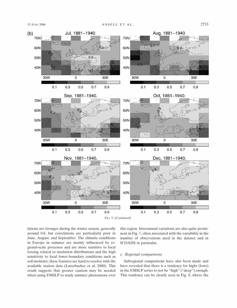
During 1881–1940 (Fig. 5), the variance explainedincreases, particularly during summer and over theocean. The Middle East region, however, remains aregion of low explained variance. EMSLP contains no

FIG. 4. (a) January–June monthly gridpoint squared correlation (r2) between EMSLP and ADVICE calculated over 1850–80. (b)Same as in (a), but for July–December.


station or J86 observations in this region for 1881–98and only limited records for Beirut and Alexandria in1876–81, whereas ADVICE (as noted above) includesdata from Cairo and Jerusalem. In the last period ex-amined, 1941–95 (not shown), r2 values increaseslightly.

Given that ADVICE and EMSLP are not strictlyindependent, we also present the grid point squaredcorrelation (r2) with ERA-40. These r2 values are veryhigh, with explained variances over much of the regionin excess of 90% (the July–December values are shown

in Fig. 6). The exception is in North Africa and theMiddle East during April–November. This is mostmarked in August–September, when the variance ex-plained drops to around 10% in North Africa. The dif-ferences may be a result of the diurnal cycle correctionbeing incorrectly applied to the EMSLP product in thisarea where the true signal is small. Incorrect applica-tion could have resulted from unrecorded temporalvariations in the times of land station observations usedin the J86 fields, which were a major input to EMSLP inthis area. Differences between the two products, as a

FIG. 4. (Continued)

15 JUNE 2006 A N S E L L E T A L . 2731

result of observing times, are expected (as noted above)to be less notable over the marine regions given thegood coverage of ship observations throughout the day;r2 values are indeed high over the ocean. The poorerresult over North Africa may also indicate differencesin the number of observations in this region.

Following Jones et al. (1999), we comparedADVICE and EMSLP by calculating spatial correla-tion coefficients over the common area for 1850–1995(Fig. 7). Jones et al. (1999) note that anomalies shouldbe used to avoid artificially high correlations due to the

climatological average spatial distribution of high andlow pressure over the European–North Atlantic region.To give equal weight to the less variable lower latitudesand the more variable higher latitudes, we formed nor-malized anomalies by removing a 1961–90 average anddividing by the standard deviation, also calculated overthis period. As expected, correlations are sometimespoor during the early period, but gradually improvetoward the late twentieth century with an increasingnumber of observations (also plotted in Fig. 7). Owingto the existence of stronger anomalies in winter, corre-

FIG. 5. (a) Same as in Fig. 4, but over 1881–1940.


lations are stronger during the winter season, generallyaround 0.8, but correlations are particularly poor inJune, August, and September. The climatic conditionsin Europe in summer are mainly influenced by re-gional-scale processes and are more sensitive to localforcing related to insolation distributions and the highsensitivity to local lower-boundary conditions such assoil moisture; these features are hard to resolve with theavailable station data (Luterbacher et al. 2000). Thisresult suggests that greater caution may be neededwhen using EMSLP to study summer phenomena over

this region. Interannual variations are also quite promi-nent in Fig. 7, often associated with the variability in thenumber of observations used in the dataset and inICOADS in particular.

c. Regional comparisons

Subregional comparisons have also been made andhave revealed that there is a tendency for highs (lows)in the EMSLP series to not be “high” (“deep”) enough.This tendency can be clearly seen in Fig. 8, where the

FIG. 5. (Continued)

15 JUNE 2006 A N S E L L E T A L . 2733

EMSLP pressures are plotted against the correspond-ing ADVICE pressures for the same 31-yr period. Astraight line representing EMSLP � ADVICE values isalso plotted. We suspect that this is a consequence ofthe “smoothing” and “in-filling” procedure appliedwhen gridding the marine observations (subsection of2b). It may also be partly due to the application ofRSOI, which tends to produce damped fields, despiteour attempts to reduce this by blending back in theobservations (subsection of 3b). A similar relationshipto that seen in Fig. 8 is evident during 1881–1920, 1921–60, and 1961–2000 (not shown), indicating that it is apersistent feature of the EMSLP product. We have alsoseen this dampening when comparing the nearest gridpoint value from EMSLP with the original station se-ries. A monthly analysis of extreme events (not shown)indicated that the flattening appears not to have a ma-jor impact on these time scales.

In Fig. 9 we plot the winter North Atlantic Oscilla-tion (NAO) using EMSLP and the monthly HadSLP2product (Allan and Ansell 2006), taking the grid pointnearest to Ponta Delgada in the Azores minus thegrid point nearest Reykjavík, Iceland. Seasonal aver-ages are formed for each year and the differencesare standardized by removing a 1961–90 mean. Alsoplotted is a station-based index using data from theAzores and Reykjavík (data available online at http://www.cru.uea.ac.uk/cru/data/nao.htm). All three seriescompare well; the correlation coefficient for EMSLPand HadSLP2 is 0.97 and is 0.98 for EMSLP andthe station series. There is a lot of interannual variabil-ity evident in the NAO series, and encouragingly, de-spite the smoothing described above, EMSLP has thecorrect magnitude. This may be a result of the influenceof the Icelandic and limited Azores station data onEMSLP.

FIG. 6. Same as in Fig. 4b, but between EMSLP and ERA-40 over 1959–2001.


FIG. 7. Time series of spatial correlations for January–December between EMSLP and ADVICE. Correlation coefficients (solid line)are plotted for 1850–2003 with the scale on the left-hand axis. Also plotted is the average number of observations in each grid box foreach month (dashed line) with the scale on the right-hand axis.

15 JUNE 2006 A N S E L L E T A L . 2735

d. Variability

A general feature of least squares objective analysesis a reduction in variance and this is evident in theEMSLP reconstructed fields. It is most prominent inthe data-sparse regions (e.g., northwest Greenland andnortheast European Russia, in the far northeast of theEMULATE region). We plot daily variability withinthe summer season by calculating the standard devia-tion of all JJA daily fields for each of the 10 decades ofthe dataset (1850–1950) in Fig. 10. For the first 3 de-cades, the variability off the west Greenland coast andNewfoundland is lower than during the rest of the pe-riod. This region and period correspond to locationswith virtually no observations before blending with theJ86 fields in 1881.

During 1875–80, we have very sporadic records fromNuuk (64.16°N, 51.75°W). In 1894, the Tasiilaq (Am-masalik), Greenland, record (65.60°N, 37.63°W) begins.Nuuk and Tasiilaq are the only two Greenland stationsincluded in the dataset, besides those implicit in the J86product. Complete monthly data are available for Nuukfrom 1866, but we were unable to locate the completedaily records. The inclusion of the Nuuk station in 1875resulted in an increase of variability on the coast. It isalso much higher over central Greenland during thisdecade.

Over much of Europe and the subtropical AtlanticOcean, where coverage is better, less-marked changesare observed. However, over most of the central andnorthwest Atlantic, the variability is lower in the 1860sthan in the earlier decade, particularly off Newfound-land. While the number of marine observations is con-sistently lower during 1850–80 than subsequently, theydid not increase steadily over this 30-yr period. In fact,the 1860s were a relatively data-poor period, owing tothe American Civil War and a general decline in theMaury collection (changes in the number of observa-tions are shown in Fig. 7). This may account for thegreater reduction in variability during this periodcompared with the slightly more data-rich period of1850–60.

There is little that can be done to adjust the lowvariance; however, error estimates produced with theRSOI solution can be used to place error bars. Indeed,very large errors and uncertainty are associated withthe period before 1881 near northwest Greenland. Theerrors decrease in 1875 with the inclusion of the Nuukobservations.

FIG. 9. The winter (December–February) NAO for 1850–2003 from EMSLP (red) andHadSLP2 (blue) gridded products. The winter NAO is calculated by taking the differencebetween the grid point closest to Ponta Delgada and that closest to Reykjavík. The 1961–90mean series value is then removed from each value. Also plotted is a station-based index from1866–2003 (green), using data from Reykjavík and Ponta Delgada. Differences between thetwo station series are formed and the 1961–90 average is also removed. Correlation coeffi-cients are also given.

FIG. 8. Monthly EMSLP MSLP ( y axis) vs ADVICE MSLP (xaxis) at 45°N, 10°E for 1850–80. A straight line representingmonthly EMSLP � ADVICE is also shown.


Fig 9 live 4/C

FIG. 10. Daily variability observed within the summer season (JJA) in each decade (from 1850–1949) in EMSLP. Contours arein hPa.

15 JUNE 2006 A N S E L L E T A L . 2737

e. Extreme events

Recent extreme climate events such as the 2003 heatwave in Europe (Trigo et al. 2005; Fink et al. 2004;Schär et al. 2004; Luterbacher et al. 2004; Stott et al.2004) that significantly affect human health (Kovats etal. 2004; Koppe et al. 2004; Stéphan et al. 2005) have ledclimatologists to question whether such events are un-precedented in the historical record. EMSLP provides aunique opportunity to explore the circulation patternsassociated with both daily and submonthly extremeevents back to the mid-nineteenth century.

Following Burt (2004), we are now able to plot theatmospheric circulation conditions associated with theextreme U.K. heat waves of July 1868, July 1881, Au-gust–September 1906, August 1911, July 1923, and Au-gust 2003 using EMSLP. In Fig. 11, we plot the anoma-lous MSLP field for the days corresponding to the high-est temperatures of the summer, equal to or exceeding35°C. The years 1911 and 2003 were also anomalouslywarm summers over central Europe (e.g., Pfister 1999;Luterbacher et al. 2004). Anomalously high pressurecentered over or near southern Scandinavia is a com-mon feature in all six events, resulting in anomaloussoutheasterly flow bringing hot continental air into the

United Kingdom. Much of central Europe is dominatedby high pressure associated with these events (Fig. 11).

This circulation pattern and anomalous flow has beenidentified previously by Maryon et al. (1982) in a clus-ter analysis of summer (JA) 15-day average MSLPfields for the Northern Hemisphere. A similar analysisof both daily and 5-day fields with EMSLP and modelanalyses, as part of EMULATE, has revealed a similarcirculation type.

EMSLP also enables us to examine the circulationpatterns associated with recent U.K. floods, such as inautumn 2000, in the context of historical events. Thethree wettest Octobers in the United Kingdom andWales during 1766–2003 were in 1903, 2000, and 1987(Jones and Conway 1997; Alexander and Jones 2001).Using U.K. daily weather records and a chronology ofBritish hydrological events (see online at http://www.dundee.ac.uk/geography/cbhe/), we have selected daysassociated with flooding in the United Kingdom foreach of these extreme months, in addition to 3 nine-teenth-century flooding events: 1882, 1870, and 1872.These three were the 8th, 13th, and 21st wettest Octo-bers, respectively. The anomalous circulation condi-tions are plotted in Fig. 12. While all events are domi-

FIG. 11. MSLP anomalies for six heat wave events over the United Kingdom. The MSLP average anomaly is plotted for the hottestdays, where 35°C or more was reached (after Burt 2004). Anomalies are formed by removing a 1961–90 climatological average; contoursare in 2 hPa.


nated by anomalously low pressure over the UnitedKingdom, arguably of more interest are the differencesin the Nordic region and over northwest Russia.Anomalously high pressure dominates this region in2000, 1882 and 1872, whereas during 1870, 1903, and1987, negative pressures extending into Norway andparts of Sweden are prominent. EMSLP is now beingused to examine circulation changes associated withchanges in extreme storms over the United Kingdom(L. V. Alexander 2005, personal communication).

5. Conclusions

We have described the development of a daily grid-ded European–North Atlantic MSLP dataset for 1850–2003 on a 5° latitude by longitude grid, produced with86 continental and island station records and ship ob-servations from the ICOADS database. The EMSLPfields for 1850–80 are based purely on the land stationdata and ship observations. From 1881, the blendedland and marine fields are combined with already avail-able adjusted daily J86 fields, using a technique thatreduces the effect of any remaining heterogeneities in

these fields. Thus, EMSLP provides 154 yr of homog-enized pressure fields. Comparisons with other histori-cal products, such as ADVICE (Jones et al. 1999), andrecent analyses, such as ERA-40, indicate that EMSLPis able to reproduce climatological features well andexplain over 90% of the variance over much of theEMULATE region.

Three main issues, however, have been highlighted.First, smoothing applied during the gridding and qual-ity control procedure has “flattened” the daily fields.Nevertheless, the seasonal NAO index calculated fromEMSLP appears to have the correct magnitude (Fig. 9)and the flattening appears not to have a major impacton a monthly analysis of extreme events (not shown).

Second, during the data-sparse period of 1850–80, thevariance to the far east and far west of the EMULATEregion is notably lower than after 1880. This is a con-sequence of the RSOI procedure and data sparseness.While it is difficult to correct this problem, error esti-mates produced with the OI solution can be employedto flag unreliable values. This result highlights the needto digitize the millions of observations that are stillavailable from ship logbooks held in the U.K. National

FIG. 12. MSLP anomalies for six flooding events over the United Kingdom. Days were selected in each case from daily station totals,available in the U.K. DWRs held in the U.K. Meteorological Library and with reference to historical flooding events are available fromthe Chronology of British Hydrological Events (http://www.dundee.ac.uk/geography/cbhe/). Anomalies are formed by removing a1961–90 climatological average; contours are in 4 hPa.

15 JUNE 2006 A N S E L L E T A L . 2739

Archives in Kew and the National Maritime Museum inGreenwich, and land station records available in dailyweather record volumes held in the Met Office ar-chives.

Third, again during the data-sparse period notedabove, the pressures over Greenland appear to be toohigh in winter. We suggest that this is due to the use ofNCEP–NCAR reanalysis data in the reconstruction ofthe MSLP fields. It is not a direct result of the highpressure bias over Greenland in the NCEP–NCAR re-analysis in winter, because the reconstruction ofEMSLP uses the covariance matrix of NCEP MSLPanomalies. Rather, we argue that this bias is due to theNCEP fields being too variable over Greenland [seen incomparisons with ERA-40 (not shown)], resulting inslightly positive MSLP anomalies (via the covariancematrix) over the high-altitude northwest Atlantic in thisperiod, yielding strong positive MSLP anomalies overGreenland.

Despite these issues, we believe EMSLP is suitablefor characterizing circulation patterns over the Europe-an–North Atlantic region. While the existing J86 fields,derived from synoptic hand-drawn charts, providegreater detail than EMSLP, they contain heterogene-ities (see Jones 1987), arising in particular from changesin source (detailed in Table 3). As a result, EMSLP,being homogenized, is more suitable for extendedanalyses back to the nineteenth century. For more re-cent (post 1970) analyses of synoptic events or cyclonetracking studies, we suggest that reanalysis productswould be more suitable. However, we were able to ex-amine the anomalous conditions during the recent 2003heat wave in Europe (Fig. 11) and recent floodingevents (Fig. 12) in a historical context.

Using EMSLP, the next stage of EMULATE will beto fully examine whether relationships between SSTand circulation patterns are stationary. EMSLP, its as-sociated error estimates, and number of observationfields will be freely available online after November2005 (www.cru.uea.ac.uk/cru/projects/emulate/).

Acknowledgments. We wish to thank Pat Folland andGail Willetts for their help in digitizing many of the MetOffice holdings of daily weather records. We also wishto thank Rudolf Brazdil for kindly providing the dailyseries for Prague, Aiguo Dai for providing the diurnalcycle phase and amplitude fields, and Gil Compo, ScottWoodruff, and Hendrik Wallbrink for many valuablediscussions with regards to the duplicates and lowMSLP bias issue in ICOADS. We are extremely grate-ful for help and advice from Alexey Kaplan in applyingRSOI. We recognize the individual efforts of M. Rod-well and D. Wheeler, T. Brandsma, and M. Barriendos

in obtaining data for Gibraltar, De Bilt, and Paris andPalmero, respectively. This project was funded by theEuropean Commission under Contract EVK2.CT2002-00161. Mariano Barriendos’s work was done underContract “Programa Ramon y Cajal.” E. Xoplaki and J.Luterbacher are further supported by NCCR Climate.Finally, we thank three anonymous reviewers for thehelpful comments and suggestions. This work is Britishcrown copyright.

APPENDIX A

Undetected Duplicates

We were advised (G. Compo 2003, personal commu-nication) that there were a number of undetected (andhence unflagged) duplicates in the ICOADS database.These arose because in some cases, the gravity correc-tion has been applied in reverse to the MSLP data ob-tained from one particular deck of data (deck 156).Another deck (193) contained many data at the sameposition (within ��0.1°) as the deck 156 data and withidentical values for SST, air temperature, etc., but withpressures different by twice the gravity correction. Thisonly happened in certain months and so this may be theresult of the error of one particular digitizer. This is arelatively easy problem to correct when there are coin-cident data from deck 193 with which to compare thedeck 156 data, and a fix was developed to exclude theerroneous data from deck 156. However, there aremany areas for which there are deck 156 data, but nodeck 193 data; and deck 156 carries on after 1938 whendeck 193 ends. These nonduplicate deck 156 data havebeen compared with other neighboring (but not coin-cident) values from other decks (e.g., 207, 116, 155, 110)during the 1940s, and no evidence of undetected dupli-cates was found. This is consistent with the belief thatthis problem does not persist beyond 1938 (S. Woodruff2003, personal communication).

APPENDIX B

Correcting for the Low MSLP Bias in U.S. MauryObservations

The 1850s decade in the ICOADS data is dominatedby anomalously low MSLP over much of the globalocean. This signal is strongest in midlatitude regions.Such a large and coherent signal was not seen duringany other decade and was not supported by land-baseddata. It was first reported by Todd Mitchell in 2002 at aworkshop on the use of historical marine climate data(Diaz et al. 2002), and remains an unresolved problemwithin the ICOADS pressure community. During1850–55, the only data source was deck 701 (the U.S.


Maury collection). After 1855, observations from theNetherlands deck 193 begin and the low bias is lessprominent. Because EMULATE required fields tostart in 1850, it was not possible to simply ignore theU.S. Maury observations.

The marine gridding procedure works with residualsby removing a reference monthly background fieldvalue based on 1850–2003 from each observation (seethe subsection of 2b). The deck 701 observations areanomalously negative compared with these backgroundfields, but if we create residuals by removing a back-ground based on just the biased deck 701 observations,the residuals are smaller in magnitude. So a deck 701monthly background climatology was created by aver-aging deck 701 gridded fields for only 1850–60. Thegridding and quality control procedure was rerun, nowusing two reference monthly background fields: the“normal” monthly 1850–2003 background and the deck701 monthly climatology. If an observation was fromdeck 701, the 701 climatology was removed; the normalmonthly background field was removed from all otherobservations. After the daily median residual wasformed on the 1° � 1° grid, the normal monthly back-ground value was added back.

By incorporating this procedure, a marked reductionin the low MSLP bias was observed. When comparingthe 1850–60 decade to a 1961–90 climatology, theMSLP over the North Atlantic region remained anoma-lously low, though this signal was weaker than was ob-served in an earlier uncorrected version of the EMSLPdataset. Our procedure will have removed any realmultiannual climate anomaly during 1850–55, but com-parisons with land-based data support our treatment ofthe marine data.

REFERENCES

Alexander, L. V., and P. D. Jones, 2001: Updated precipitationseries for the U.K. and discussion of recent extremes. Atmos.Sci. Lett., 1, doi:10.1006/asle.2000.0016.

Alexandersson, H., 1986: A homogeneity test applied to precipi-tation data. Int. J. Climatol., 6, 661–675.

Allan, R. J., and T. J. Ansell, 2006: A new globally completemonthly historical gridded mean sea level pressure dataset(HadSLP2): 1850–2004. J. Climate, in press.

Basnett, T., and D. E. Parker, 1997: Development of the GlobalMean Sea Level Pressure Data Set GMSLP2. CRTN 79,Hadley Centre, Met Office, 16 pp.

Board of Trade, 1863: Meteorological Papers (Board of Trade).No. 1, 2d ed. Her Majesty’s Stationary Office, London,United Kingdom, 84 pp.

Boletin Meteorologico Diario, 1875: Spanish Daily WeatherRecords.

Burt, S., 2004: The August 2003 heatwave in the United Kingdom:Part 1—Maximum temperatures and historical precedents.Weather, 59, 199–208.

Camuffo, D., and P. Jones, 2002: Improved Understanding of PastClimatic Variability from Early Daily European InstrumentalSources. Kluwer Academic, 392 pp.

Caswell, A., 1859: Meteorological observations made at Provi-dence, R. I. extending over a period of twenty-eight years anda half from December 1831–May 1860. Smithsonian Contri-butions to Knowledge, Vol. 12, No. 103, Smithsonian Institu-tion, Washington, DC, 179 pp.

Chapman, S., and R. S. Lindzen, 1970: Atmospheric Tides. D.Reidel, 200 pp.

Dai, A., and J. Wang, 1999: Diurnal and semidiurnal tides inglobal surface pressure fields. J. Atmos. Sci., 56, 3874–3891.

Diaz, H., C. K. Folland, T. Manabe, D. E. Parker, R. Reynolds,and S. Woodruff, 2002: Workshop on advances in the use ofhistorical marine climate data. CLIVAR Exchanges, No. 25,International CLIVAR Project Office, Southampton, UnitedKingdom, 71–73.

Fink, A. H., T. Brücher, A. Krüger, G. C. Leckebusch, J. G. Pinto,and U. Ulbrich, 2004: The 2003 European summer heatwavesand drought—synoptic diagnosis and impacts. Weather, 59,209–216.

Hickey, K., P. Dunlop, K. Hoare, and F. Gaffney, 2003: WeatherDiary 1861–1966 and Daily, Monthly, Seasonal and AnnualPressure 1861–1920. Vol. 1, Meteorological Data Recorded atNational University of Ireland, Galway, Department of Ge-ography, National University of Ireland, 81 pp.

Jackson, M., 1986: Operational superfiles. Met Office Tech. Note25, 41 pp.

Jones, P. D., 1987: The early twentieth century Arctic high—factor fiction? Climate Dyn., 1, 63–75.

——, and D. Conway, 1997: Precipitation in the British Isles: Ananalysis of area-average data updated to 1995. Int. J. Clima-tol., 17, 427–438.

——, T. Jónsson, and D. Wheeler, 1997: Extension to the NorthAtlantic Oscillation using early instrumental pressure obser-vations from Gibraltar and south-west Iceland. Int. J. Clima-tol., 17, 1433–1450.

——, and Coauthors, 1999: Monthly mean pressure reconstruc-tions for Europe for the 1780–1995 period. Int. J. Climatol.,19, 347–364.

Kalnay, E., and Coauthors, 1996: The NCEP/NCAR 40-Year Re-analysis Project. Bull. Amer. Meteor. Soc., 77, 437–471.

Kaplan, A., Y. Kushnir, M. A. Cane, and M. B. Blumenthal, 1997:Reduced space optimal analysis for historical datasets: 136years of Atlantic sea surface temperatures. J. Geophys. Res.,102 (C13), 27 835–27 860.

——, ——, and ——, 2000: Reduced space optimal interpolationof historical marine sea level pressure: 1854–1992. J. Climate,13, 2987–3002.

Kington, J. A., 1980: Daily weather mapping from 1781. ClimaticChange, 3, 7–36.

——, 1988: The Weather of the 1780s over Europe. CambridgeUniversity Press, 166 pp.

Koppe, C., R. S. Kovats, G. Jendritzky, and B. Menne, 2004:Heat-waves: Risks and responses. Health and Global Envi-ronmental Change Series, Vol. 2, WHO Regional Office forEurope, 123 pp.

Kovats, R. S., S. Hajat, and P. Wilkinson, 2004: Contrasting pat-terns of mortality and hospital admissions during hot weatherand heat waves in Greater London, UK. Occup. Environ.Med., 61, doi:10.1136/oem.2003.012047.

Lamb, H. H., and A. I. Johnson, 1966: Secular variations of the

15 JUNE 2006 A N S E L L E T A L . 2741

atmospheric circulation since 1750. Geophys. Mem. 110, MetOffice, 125 pp.

Luterbacher, J., and Coauthors, 2000: Reconstruction of monthlymean sea level pressure over Europe for the Late MaunderMinimum period (1675–1715). Int. J. Climatol., 20, 1049–1066.

——, and Coauthors, 2002: Reconstruction of sea level pressurefields over the Eastern North Atlantic and Europe back to1500. Climate Dyn., 18, doi:10.1007/s00382-001-0196-6.

——, D. Dietrich, E. Xoplaki, M. Grosjean, and H. Wanner, 2004:European seasonal and annual temperature variability,trends, and extremes since 1500. Science, 303, 5663,doi:10.1126/science.1093877.

Maryon, R. H., A. M. Storey, and D. Carr, 1982: A multivariatelong range forecasting model. Met Office Branch Memo. 106,48 pp.

Meteorological Office, 1890: Meteorological observations at theforeign and colonial stations of the Royal Engineers and theArmy Medical Department, 1852–1886. Met Office Rep. 83,London, United Kingdom, 261 pp.

Parker, D. E., 1984: The statistical effects of incomplete samplingof coherent data series. J. Climatol., 4, 445–449.

Pfister, C., 1999: Wetternachhersage: 500 Jahre Klimavariationenund Naturkatastrophen (1496-1995). Haupt, 304 pp.

Rayner, N. A., D. E. Parker, E. B. Horton, C. K. Folland, L. V.Alexander, D. P. Rowell, E. C. Kent, and A. Kaplan, 2003:Global analyses of sea surface temperature, sea ice, and nightmarine air temperature since the late nineteenth century. J.Geophys. Res., 108, 4407, doi:10.1029/2002JD002670.

Razuvaev, V. N., E. G. Apasova, and R. A. Martuganov, 1998:Six- and three-hourly meteorological observations from 223U.S.S.R. Stations. CDIAC-108, NDP-048, Carbon DioxideInformation Analysis Center, Oak Ridge National Labora-tory, 137 pp.

Reynolds, R. W., 1988: A real-time global sea surface temperatureanalysis. J. Climate, 1, 75–86.

Schär, C., P. L. Vidale, D. Lüthi, C. Frei, C. Häberli, M. Liniger,and C. Appenzeller, 2004: The role of increasing temperature

variability in European summer heat waves. Nature, 427,doi:10.1038/nature02300.

Schmith, T., H. Alexandersson, K. Iden, and H. Tuomenvirta,1997: North Atlantic–European pressure observations 1868–1995 (WASA dataset version 1.0). Danish MeteorologicalInstitute Tech. Rep. 97-3, 13 pp.

Shapiro, R., 1971: The use of linear filtering as a parameterizationof atmospheric diffusion. J. Atmos. Sci., 28, 523–531.

Simmons, A. J., and Coauthors, 2004: Comparison of trends andlow-frequency variability in CRU, ERA-40, and NCEP/NCAR analyses of surface air temperature. J. Geophys. Res.,109, D24115, doi:10.1029/2004JD005306.

Slonosky, V. C., 2003: The meteorological observations of Jean-François Gaultier, Quebec, Canada: 1742–56. J. Climate, 16,2232–2247.

——, P. D. Jones, and T. D. Davies, 1999: Homogenization tech-niques for European monthly mean surface pressure series. J.Climate, 12, 2658–2672.

——, ——, and ——, 2001: Instrumental pressure observationsand atmospheric circulation from the 17th and 18th centuries:London and Paris. Int. J. Climatol., 21, 285–298.

Stéphan, F., S. Ghiglione, F. Decailliot, L. Yakhou, P. Duvaldes-tin, and P. Legrand, 2005: Effect of excessive environmentalheat on core temperature in critically ill patients. An obser-vational study during the 2003 European heat wave. Br. J.Anaesth., 94, doi:10.1093/bja/aeh291.

Stott, P. A., D. A. Stone, and M. R. Allen, 2004: Human contri-bution to the European heatwave of 2003. Nature, 432,doi:10.1038/nature03089.

Trigo, R. M., R. García-Herrera, J. Díaz, I. F. Trigo, and M. A.Valente, 2005: How exceptional was the early August 2003heatwave in France? Geophys. Res. Lett., 32, L10701,doi:10.1029/2005GL022410.

Woodruff, S. D., R. J. Slutz, R. L. Jenne, and P. M. Steurer, 1987:A Comprehensive Ocean–Atmosphere Data Set. Bull. Amer.Meteor. Soc., 68, 1239–1250.

Worley, S. J., S. D. Woodruff, R. W. Reynolds, S. J. Lubker, andN. Lott, 2005: ICOADS release 2.1 data and products. Int. J.Climatol., 25, 823–842.


Daily Mean Sea Level Pressure Reconstructions for the ...

Documents