D6122

Designation: D 6122 – 99 An American National Standard

Standard Practice forValidation of Multivariate Process InfraredSpectrophotometers 1

This standard is issued under the fixed designation D 6122; the number immediately following the designation indicates the year oforiginal adoption or, in the case of revision, the year of last revision. A number in parentheses indicates the year of last reapproval. Asuperscript epsilon (e) indicates an editorial change since the last revision or reapproval.

1. Scope

1.1 This practice covers requirements for the validation ofmeasurements made by on-line, process near- or mid-infraredanalyzers, or both, used in the calculation of physical, chemi-cal, or quality parameters of liquid petroleum products. Theparameters are calculated from spectroscopic data using mul-tivariate modeling methods. The requirements include verifi-cation of adequate instrument performance, verification of theapplicability of the calibration model to the spectrum of thesample under test, and verification of equivalence between theresult calculated from the infrared measurements and the resultproduced by the primary method used for the development ofthe calibration model.

1.2 This practice does not cover procedures for establishingthe calibration model used by the analyzer. Calibration proce-dures are covered in Practices E 1655 and references therein.

1.3 This practice is intended as a review for experiencedpersons. For novices, this practice will serve as an overview oftechniques used to verify instrument performance, to verifymodel applicability to the spectrum of the sample under test,and to verify equivalence between the parameters calculatedfrom the infrared measurement and the results of the primarymethod measurement.

1.4 This practice teaches and recommends appropriate sta-tistical tools, outlier detection methods, for determiningwhether the spectrum of the sample under test is a member ofthe population of spectra used for the analyzer calibration. Thestatistical tools are used to determine if the infrared measure-ment results in a valid property or parameter estimate.

1.5 The outlier detection methods do not define criteria todetermine whether the sample, or the instrument is the cause ofan outlier measurement. Thus, the operator who is measuringsamples on a routine basis will find criteria to determine that aspectral measurement lies outside the calibration, but will nothave specific information on the cause of the outlier. Thispractice does suggest methods by which instrument perfor-mance tests can be used to indicate if the outlier methods areresponding to changes in the instrument response.

1.6 This practice is not intended as a quantitative perfor-mance standard for the comparison of analyzers of differentdesign.

1.7 Although this practice deals primarily with validation ofon-line, process infrared analyzers, the procedures and statis-tical tests described herein are also applicable to at-line andlaboratory infrared analyzers which employ multivariate mod-els.

1.8 This standard does not purport to address all of thesafety concerns, if any associated with its use. It is theresponsibility of the user of this standard to consult andestablish appropriate safety and health practices and deter-mine the applicability of regulatory limitations prior to use.

2. Referenced Documents

2.1 ASTM Standards:D 1265 Practice for Sampling Liquefied Petroleum Gases2

D 3764 Practice for Validation of Process Stream Analyz-ers3

D 4057 Practice for Manual Sampling of Petroleum andPetroleum Products3

D 4177 Practice for Automatic Sampling of Petroleum andPetroleum Products3

D 6299 Practice for Applying Statistical Quality AssuranceTechniques to Evaluate Analytical Measurement SystemPerformance4

E 131 Terminology Relating to Molecular Spectroscopy5

E 275 Practice for Describing and Measuring Performanceof Ultraviolet, Visible, and Near Infrared Spectrophotom-eters5

E 932 Practice for Describing and Measuring Performanceof Dispersive Infrared Spectrophotometers5

E 1421 Practice for Describing and Measuring Performanceof Fourier Transform Infrared (FT-IR) Spectrometers:Level Zero and Level One Tests5

E 1655 Practices for Infrared, Multivariate, QuantitativeAnalysis5

E 1866 Guide for Establishing Spectrophotometer Perfor-mance Tests5

E 1944 Practice for Describing and Measuring Performance1 This practice is under the jurisdiction of ASTM Committee D-2 on Petroleum

Products and Lubricants and is the direct responsibility of Subcommittee D02.25 onValidation of Process Analyzers and Statistical Quality Assurance of MeasurementProcesses for Petroleum and Petroleum Products.

Current edition approved Dec. 10, 1999. Published December 1999. Originallypublished as D 6122–97. Last previous edition D 6122–97.

2 Annual Book of ASTM Standards, Vol 05.01.3 Annual Book of ASTM Standards, Vol 05.02.4 Annual Book of ASTM Standards, Vol 05.04.5 Annual Book of ASTM Standards, Vol 03.06.

1

Copyright © ASTM, 100 Barr Harbor Drive, West Conshohocken, PA 19428-2959, United States.

of Fourier Transform Near-Infrared (FT-NIR) Spectrom-eters: Level Zero and Level One Tests5

3. Terminology

3.1 Definitions:3.2 For definitions of terms and symbols relating to IR

spectroscopy, refer to Terminology E 131.3.3 For definitions of terms and symbols relating to multi-

variate calibration, refer to Practices E 1655.3.4 Definitions of Terms Specific to This Standard:3.4.1 action limit, n—the limiting value from an instrument

performance test, beyond which the analyzer is expected toproduce potentially invalid results.

3.4.2 analyzer , n—all piping, hardware, computer, soft-ware, instrumentation and calibration model required to auto-matically perform analysis of a process or product stream.

3.4.3 analyzer calibration, n—seemultivariate calibration.3.4.4 analyzer intermediate precision, n— a statistical mea-

sure of the expected long-term variability of analyzer resultsfor samples whose spectra are neither outliers, nor nearestneighbor inliers.

3.4.5 analyzer model, n—seemultivariate model.3.4.6 analyzer repeatability, n—a statistical measure of the

expected short-term variability of results produced by theanalyzer for samples whose spectra are neither outliers nornearest neighbor inliers.

3.4.7 analyzer result, n—the numerical estimate of aphysical, chemical, or quality parameter produced by applyingthe calibration model to the spectral data collected by theanalyzer.

3.4.8 analyzer validation test,, n—seevalidation test.3.4.9 calibration transfer, n— a method of applying a

multivariate calibration developed on one analyzer to a differ-ent analyzer by mathematically modifying the calibrationmodel or by instrument standardization.

3.4.10 check sample, n—a single, pure liquid hydrocarboncompound, or a known, reproducible mixture of liquid hydro-carbon compounds whose spectrum is constant over time suchthat it can be used in a performance test.

3.4.11 control limits, n—limits on a control chart which areused as criteria for signaling the need for action, or for judgingwhether a set of data does or does not indicate a state ofstatistical control. E 456

3.4.12 exponentially weighted moving average controlchart, n—a control chart based on the exponentially weightedaverage of individual observations from a system; the obser-vations may be the differences between the analyzer result, andthe result from the primary method.

3.4.13 individual observation control chart, n—a controlchart of individual observations from a system; the observa-tions may be the differences between the analyzer result andthe result from the primary method.

3.4.14 inlier, n—seenearest neighbor distance inlier.3.4.15 inlier detection methods, n—statistical tests which

are conducted to determine if a spectrum resides within aregion of the multivariate calibration space which is sparselypopulated.

3.4.16 in-line probe, n—a spectrophotometer cell installedin a process pipe or slip stream loop and connected to the

analyzer by optical fibers.3.4.17 instrument, n—spectrophotometer, associated elec-

tronics and computer, spectrophotometer cell and, if utilized,transfer optics.

3.4.18 instrument standardization, n—a procedure for stan-dardizing the response of multiple instruments such that acommon multivariate model is applicable for measurementsconducted by these instruments, the standardization beingaccomplished by way of adjustment of the spectrophotometerhardware or by way of mathematical treatment of the collectedspectra.

3.4.19 line sample, n—a process or product sample which iswithdrawn from a sample port in accordance with PracticesD 1265, D 4057, or D 4177, whichever is applicable, during aperiod when the material flowing through the analyzer is ofuniform quality and the analyzer result is essentially constant.

3.4.20 moving range of two control chart, n— a controlchart that monitors the change in the absolute value of thedifference between two successive differences of the analyzerresult minus the result from the primary method.

3.4.21 multivariate calibration, n—an analyzer calibrationthat relates the spectrum at multiple wavelengths or frequen-cies to the physical, chemical, or quality parameters.

3.4.22 multivariate model, n—a multivariate, mathematicalrule or formula used to calculate physical, chemical, or qualityparameters from the measured infrared spectrum.

3.4.23 nearest neighbor distance inlier, n— a spectrumresiding within a gap in the multivariate calibration space, theresult for which is subject to possible interpolation error.

3.4.24 optical background, n—the spectrum of radiationincident on a sample under test, typically obtained by measur-ing the radiation transmitted through the spectrophotometercell when no sample is present, or when an optically thin ornonabsorbing liquid is present.

3.4.25 optical reference filter, n—an optical filter or otherdevice which can be inserted into the optical path in thespectrophotometer or probe producing an absorption spectrumwhich is known to be constant over time, such that it can beused in place of a check or test sample in a performance test.

3.4.26 outlier detection limits, n—the limiting value forapplication of an outlier detection method to a spectrum,beyond which the spectrum represents an extrapolation of thecalibration model.

3.4.27 outlier detection methods, n—statistical tests whichare conducted to determine if the analysis of a spectrum usinga multivariate model represents an interpolation of the model.

3.4.28 outlier spectrum, n—a spectrum whose analysis by amultivariate model represents an extrapolation of the model.

3.4.29 performance test, n—a test that verifies that theperformance of the instrument is consistent with historical dataand adequate to produce valid results.

3.4.30 physical correction, n— a type of pos processingwhere the correction made to the numerical value produced bythe multivariate model is based on a separate physical mea-surement of, for example, sample density, sample path length,or particulate scattering.

3.4.31 post-processing, v—performing a mathematical op-eration on an intermediate analyzer result to produce the final

D 6122

2

result, including correcting for temperature effects, adding amean property value of the analyzer calibration, and convertinginto appropriate units for reporting purposes.

3.4.32 pre-processing, v—performing mathematical opera-tions on raw spectral data prior to multivariate analysis ormodel development, such as selecting wave length regions,correcting for baseline, smoothing, mean centering, and assign-ing weights to certain spectral positions.

3.4.33 primary method, n—the analytical procedure used togenerate the reference values against which the analyzer is bothcalibrated and validated; Practices E 1655 uses the termreference method in place of the term primary method.

3.4.34 process analyzer system, n—seeanalyzer.3.4.35 process analyzer validation samples, n—seevalida-

tion samples.3.4.36 spectrophotometer cell, n— an apparatus which al-

lows a liquid hydrocarbon to flow between two optical surfaceswhich are separated by a fixed distance, the sample pathlength,while simultaneously allowing light to pass through the liquid.

3.4.37 test sample, n—a process or product sample, or amixture of process or product samples, which has a constantspectrum for a finite time period, and which can be used in aperformance test; test samples and their spectra are generallynot reproducible in the long term.

3.4.38 transfer optics, n—a device which allows movementof light from the spectrophotometer to a remote spectropho-tometer cell and back to the spectrophotometer; transfer opticsinclude optical fibers or other optical light pipes.

3.4.39 validation samples, n—samples that are used tocompare the analyzer results to the primary method resultsthrough the use of control charts and statistical tests; validationsamples used in the initial validation may be line and testsamples, whereas validation samples used in the periodicvalidation are line samples.

3.4.40 validated result, n—a result produced by the analyzerfor a sample whose spectrum is neither an outlier nor a nearestneighbor inlier that is equivalent, within control limits to theresult expected from the primary method, so that the result canbe used instead of the direct measurement of the sample by theprimary method.

3.4.41 validation test, n—a test performed on a validationsample that demonstrates that the result produced by theanalyzer and the result produced by the primary method areequivalent to within control limits.

4. Summary of Practice

4.1 This section describes, in summary form, the stepsinvolved in the validation of an infrared analyzer over the longterm. Before this practice may be undertaken, certain precon-ditions shall be satisfied. The preconditions are described inSection 7. This practice consists of four major procedures.

4.2 Each time a spectrum of a process sample is collected,statistical tests are performed to verify that the multivariatemodel is applicable to the spectrum. Only spectra whoseanalysis represents interpolation of the multivariate modelandwhich are sufficiently close to spectra in the calibration may beused in the analyzer validation.

4.3 When the analyzer is initially installed, or after majormaintenance is concluded, performance tests are conducted to

verify that the instrument is functioning properly. The intent ofthese tests is to provide a rapid indication of the state of theinstrument. These tests are necessary but not sufficient todemonstrate valid analyzer results.

4.4 After the initial performance test is successfully com-pleted, an initial validation test is conducted to verify that theresults produced by the analyzer are in statistical agreementwith results for the primary method. Once this initial validationis completed, the analyzer results are considered valid forsamples whose spectra are neither outliers or nearest neighborinliers.

4.5 During routine operation of the analyzer, validation testsare conducted on a regular, periodic basis to demonstrate thatthe analyzer results remain in statistical agreement with resultsfor the primary method. Between validation tests, performancetests are conducted to verify that the instrument is performingin a consistent fashion.

5. Significance and Use

5.1 The primary purpose of this practice is to permit the userto validate numerical values produced by a multivariate,infrared or near-infrared, on-line, process analyzer calibrated tomeasure a specific chemical concentration, chemical property,or physical property.The validated analyzer results are ex-pected to be equivalent, over diverse samples whose spectraare neither outliers or nearest neighbor inliers, to thoseproduced by the primary method to within control limitsestablished by control charts for the prespecified statisticalconfidence level.

5.2 Procedures are described for verifying that the instru-ment, the model, and the analyzer system are stable andproperly operating.

5.3 A multivariate analyzer system inherently utilizes amultivariate calibration model. In practice the model bothimplicitly and explicitly spans some subset of the population ofall possible samples that could be in the complete multivariatesample space. The model is applicable only to samples that fallwithin the subset population used in the model construction. Asample measurement cannot be validated unless applicability isestablished. Applicability cannot be assumed.

5.3.1 Outlier detection methods are used to demonstrateapplicability of the calibration model for the analysis of theprocess sample spectrum. The outlier detection limits are basedon historical as well as theoretical criteria. The outlier detectionmethods are used to establish whether the results obtained byan analyzer are potentially valid. The validation procedures arebased on mathematical test criteria that indicate whether theprocess sample spectrum is within the range spanned by theanalyzer system calibration model. If the sample spectrum is anoutlier, the analyzer result is invalid. If the sample spectrum isnot an outlier, then the analyzer result is valid providing that allother requirements for validity are met. Additional, optionaltests may be performed to determine if the process samplespectrum falls in a sparsely populated region of the multivari-ate space covered by the calibration set, too far from neigh-boring calibration spectra toensure good interpolation. Forexample, such nearest neighbor tests are recommended if thecalibration sample spectra are highly clustered.

5.3.2 This practice does not define mathematical criteria to

D 6122

3

determine from a spectroscopic measurement of a samplewhether the sample, the model, or the instrument is the causeof an outlier measurement. Thus the operator who is measuringsamples on a routine basis will find criteria in the outlierdetection method to determine whether a sample measurementlies within the expected calibration space, but will not havespecific information as to the cause of the outlier withoutadditional testing.

6. Apparatus and Considerations for Quantitative On-Line Process IR Measurements

6.1 Infrared or Near-Infrared Spectrophotometer:6.1.1 The analyzer covered by this practice is based on an

infrared spectrophotometer, double-beam or single-beam, suit-able for recording accurate measurements in the near-infrared(780 to 2500 nm, 12820.5 to 4000 cm–1) or mid-infrared(4000–400 cm–1) regions, or both. The spectral range measuredby the analyzer shall be the same as that of the instrument usedin collecting the spectral data upon which the multivariatecalibration model is based. Complete descriptions of theinstrumentation and procedures that are required for quantita-tive on-line process IR measurements are beyond the scope ofthis practice. Some general guidelines are given in Annex A1.(Warning—There are inherent dangers associated with the useof electrical instrumentation, on-line processes, and hydrocar-bon materials. The users of this practice should have a practicalknowledge of these hazards and employ appropriate safe-guards.)

6.1.2 In developing spectroscopic methods, it is the respon-sibility of the user to describe the instrumentation and theperformance required to achieve the desired repeatability,reproducibility, and accuracy for the application.

6.2 Process Analyzer System:6.2.1 The process analyzer system typically includes the

spectrophotometer, transfer optics, the hardware for samplehandling, the hardware for introduction of reference standardsand solvents, the computer for controlling the spectrophotom-eter and calculating results, and the multivariate model. Thesystem configuration should be compatible with the mid-infrared or near-infrared IR measurement and this practice.

6.3 Collection of Line Samples:6.3.1 Withdraw line samples in accordance with accepted

sampling methods as given by Practices D 1265, D 4057, orD 4177, whichever is applicable. Flush the entire sample loopwith the process stream sample prior to withdrawal of the linesample.

6.3.2 The intent of this practice is to collect samples thatcorrespond directly to the spectra being collected by theanalyzer. Collect the sample at a port close to the optical probeand at a time correlated with the collection of the samplespectrum. This practice requires that parameters that canimpact the result also be recorded at the time of samplecollection and the effect of these parameters be properlyaccounted for when comparing the results with the primarymethod result. For a more detailed discussion of the various lagtimes that can influence the correspondence between theanalyzer measurement and collection of line samples, seePractice D 3764.

6.3.3 Sample storage for extended time periods is not

recommended if there is a likelihood that samples degrade withtime. Chemical changes occurring during storage will causechanges in the spectrum, as well as changes in the property orquality parameter measured by the primary method.

6.3.4 If possible, at the time of line sample withdrawal,collect sufficient quantity of sample material to allow formultiple measurements of the property or quality parameter bythe primary method, should such measurements be required.

7. Preconditions

7.1 Certain preconditions shall be met before this practicecan be applied.

7.1.1 Install the analyzer in accordance with manufacturer’sinstructions.

7.1.2 Develop and validate the multivariate calibrationmodel used on the process analyzer using methods described inPractices E 1655. If a calibration transfer method is used totransfer the model from one analyzer to another, verify thetransferred model as described in Practices E 1655.

7.1.3 A quality assurance program for the primary method isrequired in order to determine the usability of values generatedby the primary method in the validation of analyzer perfor-mance using this practice (see Section 8).

8. Reference Values and the Quality Assurance Programfor the Primary Method

8.1 The property reference value against which analyzerresults are compared during validation is established by apply-ing the primary measurement method which was used in themodel development to line samples representing the processstream.

8.2 A quality assurance program for the primary method isrequired for values generated by this method to be used inanalyzer validation.

8.2.1 Carefully check the laboratory apparatus used forprimary method measurement before these tests are performedto ensure compliance with the requirements of the primary testmethod.

8.2.2 Test control materials of known composition andquality on a regularly scheduled basis. Plot the primary methodresults on control charts to ensure the long-term performanceof the primary test. Individual values, exponentially weightedmoving average, and moving range of two control charts are allrecommended for charting the performance of the primarymethod. Calculate the values for these control charts usingequations given in Sections 12 and 13. Plot the differencesbetween the primary method result, and the expected value forthe standard sample. Determine the historical precision of theprimary method from these regular tests, and compare it topublished values for the method to determine if the test iswithin expected limits. Compare the historical precision to theanalyzer precision using statistical tests.

9. Procedure

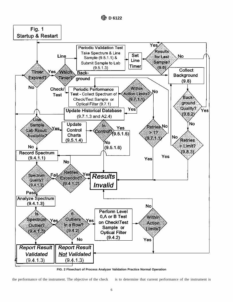
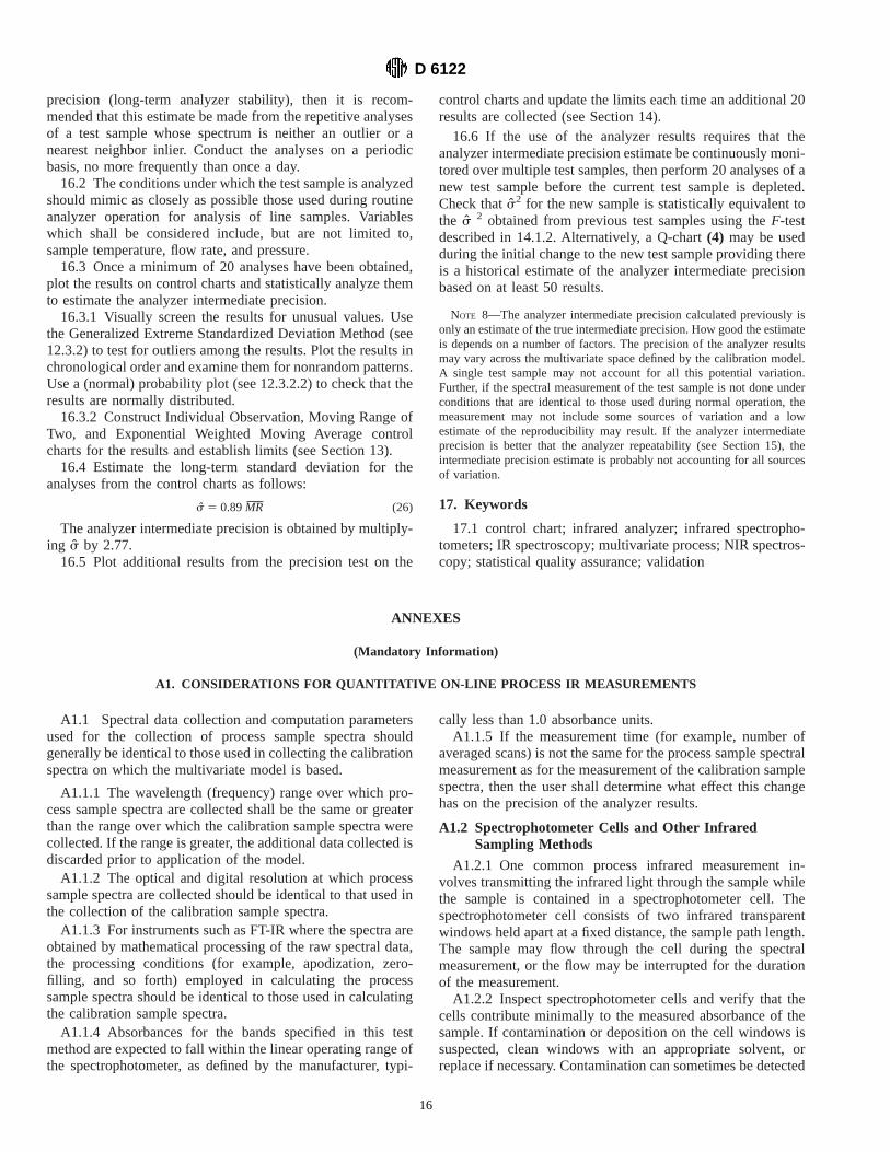
9.1 A flowchart for the steps involved in this practice isshown in Fig. 1 and Fig. 2.

9.2 Initial Performance Tests:9.2.1 After the multivariate process analyzer has been

installed (or reinstalled following major maintenance), check

D 6122

4

FIG. 1 Flowchart of Process Analyzer Validation Practice Initial Startup and Restart after Maintenance

D 6122

5

the performance of the instrument. The objective of the check is to determine that current performance of the instrument is

FIG. 2 Flowchart of Process Analyzer Validation Practice Normal Operation

D 6122

6

consistent with performance which is known to produce validanalyses. Conduct this initial check out of the instrumentwithin a short period (preferably within 24 h) after installation.Collect spectra of 20 check or test samples and analyze themusing one or more of the Level 0, Level A, or Level Bperformance tests described in Annex A2 and Practice E 1866.

9.2.2 Compare the results for the initial performance tests toperformance test action limits. These action limits may bebased on historical data for the same tests, on simulations ofthe effects of performance changes on the analyzer results, oron a combination of historical and simulated data. Methods forestablishing action limits are discussed in Annex A2 andPractice E 1866.

9.2.2.1 If the performance test results are within actionlimits, then the procedure continues with the initial validationtests. If the performance test results are not within action limits,check installation, instrument standardization or calibrationtransfer, or combination thereof, and correct the cause of theinadequate performance. Repeat the initial performance tests.

9.2.2.2 If action limits for performance tests have not beenestablished, use the results for the initial performance tests togenerate an initial historical database against which future testscan be compared, and continue the validation procedure withthe steps described in 9.3. In the absence of historical data orperformance simulations, the performance of the instrumentcannot be verified, but shall be assumed. Should the analyzerfail to validate, inadequate instrument performance could beresponsible.

9.3 Initial Validation (see Section 12 for details):9.3.1 Once the initial performance tests are completed,

collect spectra of 20 line and test samples and analyze themusing the multivariate model. In order for the results to be usedin the initial validation test, the spectra of the 20 line or testsamples shall not be either outliers or nearest neighbor inliers(see Section 11 and Annex A3). Replace samples whose spectraare outliers or nearest neighbor inliers with other line or testsamples.

9.3.2 Withdraw line samples from the process using meth-ods described in Practices D 1265, D 4057, or D 4177, which-ever is applicable, and analyze them by the primary method.The line sample shall correspond directly to the spectrumcollected in 9.3.1.

9.3.3 Check that the standard deviation of the analyzerresults for the 20 validation samples is at least 72 % of thereproducibility of the primary method for each property/component being modeled. If not, collect spectra of additionalline or test samples, or both, until the standard deviation isadequate.

9.3.4 Compare values calculated by the analyzer to thoseobtained by the primary method using statistical tests describedin Section 12. If the values are within statistical agreement,then the analyzer results are considered valid, and the analyzercan be used to analyze line samples. If the values are not withinstatistical agreement, then the installation, instrument standard-ization or calibration transfer, or combination thereof, arechecked and corrected, and the procedure starts over withinitial performance tests as described in 9.2.

9.4 Normal Operation:

9.4.1 Once the initial analyzer system validation is com-pleted, normal operations for analysis of process samples maybe conducted. Conduct tests of the performance of the analyzerand of the validity of the analyzer results on a periodic,regularly scheduled basis. When these tests are not scheduled,the normal application of the analyzer for on-line analysisproceeds as follows:

9.4.1.1 Collect a spectrum of the process sample.9.4.1.2 Optionally, conduct tests on the spectrum in order to

determine that the quality of the spectrum is adequate for usein estimating results by way of application of the multivariatemodel. Spectrum quality tests are generally defined by theinstrument manufacturer or model developer, or both. Ifspectrum quality tests are used, allow a finite number of retrieson the spectrum collection before the analyzer is consideredinoperative, and the results produced invalid.

9.4.1.3 Analyze the spectrum using the calibration model, toproduce one or more results, possibly uncertainties in theseresults, and statistics which are used to determine if thespectrum is an outlier or nearest neighbor inlier relative to thesample population used in the development of the calibrationmodel (see Section 11 and Annex A3). If the spectrum recordedduring normal operation of the analyzer is not an outlier ornearest neighbor inlier, then the calculated property valuesproduced are considered valid as long as the analyzer qualitycontrol charts are up to date and the differences between theanalyzer results and the primary method results are withincontrol limits. If the spectrum recorded during the normaloperation of the analyzer is an outlier or nearest neighbor inlier,then the specific results associated with that spectrum areconsidered to be invalid.

9.4.2 When six successive spectra recorded during thenormal operation of the analyzer are all outliers, conductperformance tests to determine if the instrument performance iswithin action limits (see 10.3.3).

9.5 Periodic Validation Tests:9.5.1 Conduct periodic analyzer validation tests at regularly

scheduled intervals, preferably once a week (see Section 13).9.5.1.1 Simultaneously, withdraw a line sample from the

process and collect a spectrum of the process stream with theprocess analyzer.

9.5.1.2 Analyze the spectrum using the multivariate modelto produce a result, and to produce outlier and nearest neighborinlier statistics. If the spectrum is an outlier or nearest neighborinlier, it cannot be used for the validation test, and theprocedure starts over with 9.5.1.

9.5.1.3 Analyze the line sample by the primary method usedin the development of the calibration.

9.5.1.4 Compare the analyzer and primary method resultsby plotting their difference on control charts as described inSection 13.

9.5.1.5 If the difference is within control limits, then thepredicted result for the analyzer is considered to be valid.

9.5.1.6 If the difference is not within control limits, then theresult for the analyzer are invalid. Check the control charts forthe primary method (see Section 8) to ensure that the primarymethod is within control limits. If the primary method is notwithin control limits, determine and correct the cause of the

D 6122

7

error, and repeat the primary method test. If the primarymethod is within control limits, conduct performance tests tocheck if the instrument performance is within action limits. Ifthe instrument performance is not within action limits, serviceto the analyzer may be necessary.

9.5.2 Collect validation samples, analyze them by the pri-mary method, and compare the analyzer and primary methodresults using control charts on a periodic basis. The exactperiod between validation samples will depend on the nature ofthe analyzer application. At minimum, collect and analyze avalidation sample at least once within each seven-day period.More frequent validation testing may be appropriate forapplications where analyzers are being used to certify products.The period between validation samples should not be less thanthe typical time required to obtain the reference data by way ofthe primary method.

9.6 If the laboratory, primary method results for a linesample are not available by the time the next time sample isscheduled to be collected, then the results produced by theanalyzer are to be considered invalid until such time as theoverdue results become available and the control charts areupdated.

9.7 Performance Tests:9.7.1 It is recommended that performance tests be con-

ducted on a regularly scheduled basis, preferably daily, be-tween the periodic analyzer validation tests. The objective ofthe test is to demonstrate that the analyzer performance isconsistent between validation tests. Details on performancetests are given in Section 10, Annex A2, and Practice E 1866.

9.7.1.1 If the results for the performance tests are withinaction limits, continue operation of the analyzer.

9.7.1.2 If the results of the performance tests are not withinaction limits, then repeat the test. If the results of the repeat testare not within action limits, then the analyzer results areconsidered invalid, and the analyzer should be serviced.

9.7.1.3 If action limits have not been established for theperformance tests, it is recommended that validation tests beperformed more frequently to establish the historical databaseagainst which the limits can be set (see Annex A2 and PracticeE 1866).

9.8 Optical Backgrounds:9.8.1 Collect new optical backgrounds on a regularly sched-

uled interval, or when indicated by analyzer performanceresults.

9.8.2 Tests may be conducted on the collected opticalbackground to determine its quality. Background quality testsare generally defined by the instrument manufacturer or modeldeveloper, or both.

9.8.3 If background quality tests are used, allow a finitenumber of retries on the spectrum collection before theanalyzer is considered inoperative, and the results producedinvalid.

10. Performance Tests

10.1 Performance tests are conducted to determine whetherthe performance of the instrument (the spectrophotometer, theoptical cell, and all transfer optics in between) is adequate toproduce spectra of the quality sufficient for valid analyses.Typically, check or test samples are introduced into the

analyzer, the spectra of these samples are analyzed using theappropriate Level 0, Level A, or Level B performance test, andthe results are plotted on charts and compared to action limits.For analyzers equipped with in-line probes, it may be imprac-tical to remove the probe to conduct performance tests. Forsuch analyzers, alternative procedures described in Annex A2and Practice E 1866 may be used to conduct performance tests.Adequacy of the spectra is determined by comparison to ahistorical database of spectra of sufficient and insufficientquality. Alternatively, simulations of possible changes in in-strument performance can be used to define the performancethat is adequate for a given application. A description of Level0, A, and B tests, and of methods for setting action limits forperformance tests based on historical data and on simulations,are described in detail in Annex A2 and Practice E 1866.

10.2 When conducting the performance tests, operate theinstrument in the most stable and reproducible conditionsattainable, as defined by the manufacturer. Allow sufficientwarm-up time before the commencement of any measure-ments. If the calibration model was based on spectra ofsamples held within a specified temperature range, then allowall samples, including check and test samples, to equilibrate tothis temperature prior to spectral measurement. If possible, theoptical configuration used for measurements of test and checksamples should beidentical to that used for measurement ofline samples. If identical optical configurations are not possibledue to analyzer design, the user should recognize that theperformance tests may not measure the performance of theentire instrument. Data collection and computation conditionsshould be equivalent to those used in the collection of thespectra used in the calibration model. Introduce fresh referencematerial into the spectrophotometer cell for each measurement.Flow through the cell during the measurement is not required.Date and time stamp the spectral data used in performancetests, and store the results of the tests in a historical database.

10.3 Timing of Analyzer Performance Tests:10.3.1 Conduct performance tests on a regularly scheduled

basis, preferably daily, to test instrument performance consis-tency between validation tests. Compare the results of theperformance tests with action limits for the tests. If a signifi-cant change in the performance is observed, conduct a secondanalysis to verify the change. If the significant change inperformance is verified, mark analyzer resultsnot validateduntil the cause and effect of the change can be determined. Ifthe change in performance is not verified, conduct analyses offive additional check or test samples to demonstrate that thefirst occurrence was an anomaly, before continuing withnormal operation.

10.3.1.1 The significance of a change in instrument perfor-mance may be unknown in the absence of historical data orsimulations. In such case, more frequent validation testing maybe required to demonstrate the relationship between analyzerperformance and valid analyses. If, after a change in instrumentperformance is observed, the analyzer results remain in control,the change is not adversely effecting analyzer results. If,however, the analyzer results go out of control relative to theprimary method, the change is adversely affecting analyzerresults.

D 6122

8

10.3.1.2 If historical data or simulations exist to demon-strate that change in performance is sufficient to produceinvalid analyses, then service the analyzer to correct theproblem. Service of this type is considered major maintenance,and initial performance and validation tests are required beforeresuming analyzer operation.

10.3.2 When an analyzer is installed, or after major main-tenance has been performed, conduct 20 instrument perfor-mance tests using the check or test sample over a 24-h periodto capture any diurnal performance variations. Compare theperformance test results for the 20 samples with performancetest action limits to determine if the analyzer performance isadequate. Add the test results for the 20 analyses to thehistorical database against which future performance tests arecompared. Once these performance tests have been success-fully completed, initiate the initial validation of the analyzer.

10.3.3 If, during the course of normal operation, the spectraof six successive samples are determined to be spectral outliers(see Section 11 and Annex A3), it is recommended thatperformance tests be conducted to demonstrate that the outlierdiagnostics are responding to chemical changes in the processstream and not to changes in the instrument performance. If theresults for the performance tests are outside action limits, thenthe outlier diagnostics may be responding to instrument per-formance and the analyzer should be serviced. If the results forthe performance tests are within action limits, then the outlierdiagnostics are most likely responding to changes in theprocess which are producing materials outside the range of thecurrent calibration. If the process remains outside the range ofthe calibration for extended periods, it is recommended that theinstrument performance be verified periodically using perfor-mance tests, until such time as the process returns to a statewhere the model is again applicable. If the process has changedso as to be permanently outside the range of the calibration,then a new model should be developed following PracticesE 1655. Revalidate the analyzer with the new model followingthe procedure described herein.

10.3.4 Conduct performance tests if a bias is observedbetween the analyzer and primary method values to determineif the bias is the result of a change in instrument performance.

10.4 Reference Materials for Instrument Performance Tests:10.4.1 Check samples are generally used for conducting

performance tests. Check samples are single, pure, liquidhydrocarbon compounds or mixtures of liquid hydrocarboncompounds of definite composition. An alternate to using acheck sample is to use an actual process sample called a testsample. For systems equipped with in-line probes, opticalfilters may be used as reference materials for instrumentperformance tests.

NOTE 1—Performance tests conducted on test samples are only in-tended to check the stability of analyzer performance over time. While theanalyzer results for the test sample can be compared to the results for theprimary method, such comparisons are not a substitute for the validationtests described in Sections 12 and 13. Analyzer results for test samples canbe used in the calculation of the analyzer intermediate precision (seeSection 16).

10.4.2 Details on reference materials for instrument perfor-mance tests are given in Annex A2 and Practice E 1866.

11. Verification that the Model is Applicable to theSpectrum of the Process Stream Sample – SpectralOutlier and Nearest Neighbor Inlier Detection

11.1 The spectra of the calibration samples define a set ofvariables that are used in the calibration model. If, whenunknown samples are analyzed, the variables calculated fromthe spectrum of the unknown sample lie within the range of thevariables for the calibration, the estimated value for theunknown sample is obtained by interpolation of the model. Ifthe variables for the unknown sample are outside the range ofthe variables in the calibration model, the estimate representsan extrapolation of the model. Additionally, if the spectrum ofthe sample under test contains spectral features that were notpresent in the spectra of the calibration samples, then thesefeatures represent variables that were not included in thecalibration, and the analysis of the sample spectrum representsan extrapolation of the model.

11.2 For the purpose of this practice, an analyzer result isconsidered valid only if the analysis involves an interpolationof the multivariate calibration model. Outlier detection meth-ods are used to determine if an analysis represents an interpo-lation or an extrapolation of the multivariate model. Themathematics involved in outlier detection are described inPractices E 1655 and in Annex A3. The calculation of outlierstatistics is by necessity an integral part of the analyzersoftware since these calculations shall be conducted each timethe multivariate model is applied to a spectrum to produce aresult. Appropriate limits for outlier tests will generally be setby the calibration model developer based on statistics from thecalibration set.

11.2.1 A Mahalanobis Distance or leverage statistic is em-ployed to determine if the spectrum being analyzed representsan interpolation or extrapolation of the variable space definedby the calibration model.

11.2.2 A spectral residuals statistic is employed to detectextrapolation of the calibration model due to spectra featureswhich were not present in the spectra of the calibration set.

11.2.3 Optionally, a Nearest Neighbor Distance statistic canbe employed to determine when the spectrum being analyzedfalls in a sparsely populated region of the multivariate calibra-tion space. While analyses of such spectra represent interpola-tion of the model, there may be insufficient information in themodel to produce valid analyses for these samples. The use ofa Nearest Neighbor Distance statistic is recommended if thecalibration samples are highly clustered in the multivariatespace. It is the responsibility of the model developer todetermine if use of a Nearest Neighbor Distance statistic isappropriate. If a Nearest Neighbor Distance statistic is em-ployed, then the results for any sample whose Nearest Neigh-bor Distance exceeds the predetermined limit are consideredinvalid. Such samples are referred to as Nearest NeighborInliers.

11.3 Annex A3 discusses available outlier detection meth-ods. Further details on outlier methods and on notations used intheir calculations are in Practices E 1655. Users may substituteother outlier detection methods providing they are at least asrigorous as those described in Annex A3 and Practices E 1655.If alternative outlier detection methods are substituted, it is the

D 6122

9

user’s responsibility to demonstrate that any analyzer resultsthat are marked as invalid by the tests described herein are alsomarked as invalid by the substituted methods.

11.4 While it is generally preferable that the outlier statisticsbe generated using the same modeling method that was used togenerate the calibration model, this is not required. Forinstance, MLR models do not provide spectral residual statis-tics. If an MLR model is used as the calibration model, anadditional PCR or PLS model may be used to provide thenecessary residuals statistics. If a supplementary model is usedto generate outlier statistics, construct the supplementarymodel using the same set of calibration samples used for thepredictive model, and apply the outlier statistics which will beused on the process analyzer system in the validation of themodel in accordance with Practices E 1655.

11.4.1 Outlier tests detect differences in the spectrum of theprocess sample relative to the spectra of the calibrationsamples. These spectral differences may be due to differencesin the chemistries of the samples, or due to differences in theperformance of the spectrometer used to collect the spectra.Table 1 discusses inferences that may be drawn from outliertest results. The outlier tests by themselves do not distinguishbetween the instrument and the sample being the cause of theoutlier result. Instrument performance tests may be used tohelp determine if the outlier test is responding to changes in theprocess or in the instrument.

12. Analyzer System Initial Validation

12.1 The initial validation of the analyzer is performed bycomparing the analyzer and primary method results for a set ofat least 20 initial validation samples. The primary methodresults are regressed against the analyzer results. A statisticaltest is performed on the regression results. The null hypothesisfor the test is that the slope of the regression line is less than orequal to zero, that is, that there is no positive correlationbetween the two sets of results. If the null hypothesis isrejected, then there is a statistically significant positive corre-lation between the two sets of results.

12.2 Initial Validation Samples:12.2.1 Initial validation of the analyzer is performed with a

minimum of 20 samples. The actual number of samples used inthe initial validation is designated byn. Spectra of these

samples must yield potentially valid results (for example, thespectra must not be outliers) as defined in Section 11. Foranalyzer validation, select samples with chemical concentra-tions or physical properties which are interpolations within therange for which the calibration was developed and validated.

12.2.2 Select initial validation samples which exhibit suffi-cient variation in the property or composition being measured.At a minimum, it is recommended that the standard deviationof the analyzer results among the initial validation samplesshould be at least 72 % of the reproducibility of the primarymethodfor each property to be measured.

NOTE 2—Seventy-two percent of the reproducibility is equivalent totwice the standard deviation of the reproducibility. Strictly speaking, thestandard deviation of both the analyzer results and the primary methodvalues are preferably at least 72 % of the reproducibility of the referencemethod to ensure that there is sufficient variation in the results to performa meaningful statistical test. However, the primary method values (seeSection 8) are not necessarily available at the time the initial validationsamples are collected. If the analyzer does not pass the initial validationtests described in 12.1, and if the standard deviation in the referencevalues is less than 72 % of the reproducibility, the user should considerrepeating the initial validation with samples that show a larger variability.

NOTE 3—If the primary method against which the analyzer results isbeing compared is not an ASTM method, the reproducibility of themethod may not be known. The repeatability of the primary method valuescan be estimated from quality assurance data (see Section 8) and used inplace of the reproducibility. The user should be aware that the repeatabilitywill generally be smaller than the reproducibility, and that 72 % of therepeatability will typically represent less variation than 72 % of theproducibility. If the analyzer does not pass the initial validation testsdescribed below, the user should consider repeating the initial validationwith samples that show a larger variability.

12.2.2.1 Samples in the required property range for validat-ing one property may not be suitable for validating anotherproperty derived from the same spectral measurement. (Forexample, three motor gasoline grades may span five octanerange but may have a constant Reid vapor pressure. Theywould, thus, be suitable for initial validation of an analyzermeasuring octane, but not Reid vapor pressure).

12.2.2.2 While line samples are preferable, the process maynot exhibit sufficient variation during the period of initialvalidation to provide the required sample variation. In thiscase, test samples that were not used for the model develop-ment may be included in the set of samples used for initialvalidation to achieve the required variation. Confirm theintegrity of these test samples by appropriate testing prior touse. Preferably, test samples should not make up more than25 % of the set of initial validation samples.

12.2.2.3 Check samples resembling the process stream maybe used in place of test samples providing that their spectra arenot outliers.

12.2.3 Initial Validation Correlation (Slope) Test—Test thecorrelation between the analyzer results, and the primarymethod results for the 20 initial validation samples by thefollowing calculation:

12.2.3.1 Perform a regression of the primary method results,Yr, versus the analyzer results,Ya. Calculate the slope of theregression,m, as follows:

m5( ~Ya – Ya!~Yr – Y r!

( ~ Ya – Ya!2 (1)

TABLE 1 Inferences Related to Outlier Detection or InstrumentFailure

MahalanobisDistance Test

SpectralResidual

Test

Inferences Status of AnalyzerResult

Less thanlimit

lessthanlimit

spectrum within range ofcalibration spectra

result valid ifcontrol charts arecurrent and within

control limitsGreater than

limitlessthanlimit

possible instrument malfunctionor model extrapolation due to

sample component outside rangefor calibration

invalid result

Less thanlimit

greaterthan limit

possible instrument malfunctionor model extrapolation due to

sample absorption not present incalibration spectra

Invalid result

Greater thanlimit

geaterthan limit

possible instrument malfunctionor model extrapolation

invalid result

D 6122

10

Y refers to meany value for then initial validation samples.12.2.3.2 Calculate the standard error of the regression co-

efficient or slope,Sm

Sm 5Œ( ~Yr – Yr!2 – m2( ~Ya – Ya!

2

~n – 2!( ~Ya – Ya!2 (2)

12.2.3.3 Calculate [m/sm] and compare the value to the 95th

percentile of Student’st distribution with ( n–2) degrees offreedom in Table 2.

12.2.3.4 If the preceding ratio exceeds thet value in thetable, the analyzer results show a statistically significantcorrelation to the reference values, and are therefore potentiallyvalid. The initial validation continues with the bias test in 12.3.

12.2.3.5 If the preceding ratio does not exceed thet value inthe table, the analyzer results do not show a statisticallysignificant positive correlation to the reference values and are,therefore, invalid. The analyzer validation process is discon-tinued until the source of the problem is identified andcorrected. If the standard deviation of either the analyzerresults or the reference values was close to 72 % of thereproducibility of the reference method, then the user mayconsider adding additional line or test samples, or both, toextend the range of initial validation set, and repeating theinitial validation correlation test.

12.3 Initial Validation Bias Test—A test is performed todetermine if there is a bias between the results for the analyzerand the primary method.

12.3.1 Compute the differences,di, between the analyzerresults and the primary method results for then initialvalidation samples

d i 5 ~ya – yr!i (3)

12.3.2 Examine then differences to determine if any areoutliers using a Generalized Extreme Standardized Deviation

Method(1).6 If any of the differences are outliers relative to thedistribution of differences, collect additional line samples toreplace them. Also examine the differences using a (Normal)Probability Plot(2) to determine if the differences are normallydistributed. The statistical quality control plots described inSection 13 assume that the differences are normally distributed.If the differences are not normally distributed, attempt todetermine the cause of the non-normal distribution and, ifpossible, correct it before restarting the validation procedure.

NOTE 4—If the multivariate model does not account for all sources ofvariation that may effect the modeled concentration or property, then thedifferences between the analyzer result and the primary method resultincludes this unmodeled variance. It is assumed that, over a sufficientlylarge, diverse set of samples, the systematic model prediction errorsresulting from this unmodeled variance will behave as if they wererandom errors, analogous to the imprecision associated with the primarymethod. If the differences are not normally distributed, then this assump-tion may be incorrect, or the set of validation samples may not be large ordiverse enough.

12.3.2.1 To detect outliers among then differences using theESD method, calculate the valuesas follows:

ESDi 5?di?/ s (4)

wheres is the standard deviation in thedi. Find the samplehaving the maximumESDi. This value isESD(1). Eliminatethis sample, recalculates, and recalculateESDi for the n-1remaining samples. Find the maximumESD i. This value isESD(2). Eliminate this sample, recalculates and recalculateESDi for the n-2 samples. Find the maximum value of theESDi. This value isESD(3). Assuming there are at most three

6 The boldface numbers in parentheses refer to the list of references at the end ofthis standard.

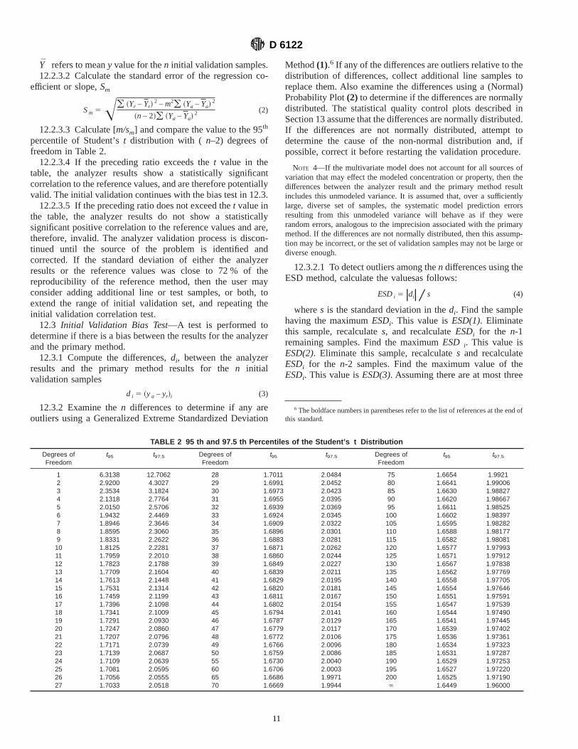
TABLE 2 95 th and 97.5 th Percentiles of the Student’s t Distribution

Degrees ofFreedom

t95 t97.5 Degrees ofFreedom

t95 t97.5 Degrees ofFreedom

t95 t97.5

1 6.3138 12.7062 28 1.7011 2.0484 75 1.6654 1.99212 2.9200 4.3027 29 1.6991 2.0452 80 1.6641 1.990063 2.3534 3.1824 30 1.6973 2.0423 85 1.6630 1.988274 2.1318 2.7764 31 1.6955 2.0395 90 1.6620 1.986675 2.0150 2.5706 32 1.6939 2.0369 95 1.6611 1.985256 1.9432 2.4469 33 1.6924 2.0345 100 1.6602 1.983977 1.8946 2.3646 34 1.6909 2.0322 105 1.6595 1.982828 1.8595 2.3060 35 1.6896 2.0301 110 1.6588 1.981779 1.8331 2.2622 36 1.6883 2.0281 115 1.6582 1.9808110 1.8125 2.2281 37 1.6871 2.0262 120 1.6577 1.9799311 1.7959 2.2010 38 1.6860 2.0244 125 1.6571 1.9791212 1.7823 2.1788 39 1.6849 2.0227 130 1.6567 1.9783813 1.7709 2.1604 40 1.6839 2.0211 135 1.6562 1.9776914 1.7613 2.1448 41 1.6829 2.0195 140 1.6558 1.9770515 1.7531 2.1314 42 1.6820 2.0181 145 1.6554 1.9764616 1.7459 2.1199 43 1.6811 2.0167 150 1.6551 1.9759117 1.7396 2.1098 44 1.6802 2.0154 155 1.6547 1.9753918 1.7341 2.1009 45 1.6794 2.0141 160 1.6544 1.9749019 1.7291 2.0930 46 1.6787 2.0129 165 1.6541 1.9744520 1.7247 2.0860 47 1.6779 2.0117 170 1.6539 1.9740221 1.7207 2.0796 48 1.6772 2.0106 175 1.6536 1.9736122 1.7171 2.0739 49 1.6766 2.0096 180 1.6534 1.9732323 1.7139 2.0687 50 1.6759 2.0086 185 1.6531 1.9728724 1.7109 2.0639 55 1.6730 2.0040 190 1.6529 1.9725325 1.7081 2.0595 60 1.6706 2.0003 195 1.6527 1.9722026 1.7056 2.0555 65 1.6686 1.9971 200 1.6525 1.9719027 1.7033 2.0518 70 1.6669 1.9944 ` 1.6449 1.96000

D 6122

11

outliers, theESDvalues are compared to criticalESDvalues inTable 3 forn samples. IfESD(3)is greater thanl3 in Table 3for n samples, then all three samples are outliers. IfESD(3)isless thanl3, but ESD(2) is greater thanl2, then the first twosamples are outliers. IfESD(3) is less thanl3 andESD(2) isless thanl2, butESD(1)is greater thanl 1, then the first sampleis an outlier. IfESD(3)is less thanl3, ESD(2)is less thanl 2

and ESD(1) is less thanl 1, then none of the samples areoutliers.

12.3.2.2 A (normal) probability plot is used to test theassumption that the differences are normally distributed. Con-struct the probability plot after outliers are eliminated in12.3.2.1. Generate a vector of probability values from 0.5/n to1- 0.5/n at intervals of 1/n. Calculate the inverse of thestandard normal cumulative distribution function at theseprobability values. Sort then differences calculated in 12.2.2.1and pair them with the inverse normal cumulative distributionfunction values. Plot these pairs as (x,y). If the differences arenormally distributed, the plot should be approximately linear.Major deviations from linearity are an indication of non-normal distributions of the differences.

12.3.2.3 Compute the bias for the initial validation processas the average difference between the analyzer results and theprimary method resultsas follows:

d 5(i51

n

di

n (5)

12.3.2.4 Calculate the variance for the validation process

Sd2 5

(i51

n

~d i – d! 2

n – 1 (6)

12.3.2.5 Computet:

t 5?d?=n

Sd(7)

12.3.2.6 Compare the computedt value with the criticaltvalues in Table 2 for (n-1) degrees of freedom.

(a) If the calculatedt value is less than or equal to the criticalt value, then the bias is not statistically significant. Theanalyzer is expected to give essentially the same average resultas the primary method, and no statistically significant biasexists and the analyzer results are valid.

(b) If the calculatedt value is greater than the criticalt value,then the bias is statistically significant. There is at least a 95 %probability that the analyzer and the primary method are notgiving the same average results. The analyzer or primarymethod validity is suspect, and further investigation of theprimary method quality assurance and the analyzer functionand operation shall be conducted to resolve the source of thebias.Bias corrections of multivariate models are not permittedwithin the scope of this practice.

NOTE 5—For the purpose of this practice, if it is necessary to add a biascorrection to a model to bring analyzer and primary method results intoagreement, the addition of the bias correction is considered to produce anew model. Validate this new model as described in Practices E 1655.Once the new model has been validated, install it on the analyzer andvalidate the analyzer performance in accordance with the proceduresdescribed herein. If the bias is changed, it again produces a new modelwhich again shall be revalidated in accordance with Practices E 1655, andthe analyzer performance shall again be validated.

12.4 Calculate the relative accuracy and precision of theinitial analyzer validation results as follows:

12.4.1 Calculate the mean square error for the analyzerresults as follows:

SEa2 5

(i51

n

~Ya – Yr!i2

n (8)

12.4.2 If there is no statistically significant bias for thevalidation process (see 12.3.2.3 to 12.3.2.6), then the 95 %confidence limit on the absolute value of the differencebetween the measurements by the validated analyzer and by theprimary method is given by

t 3 Sd (9)

wheren is the number of samples used for analyzer valida-tion, andt is the Student’st95 value from Table 2 forn degreesof freedom. This limit applies only to primary method resultsproduced by the same laboratory which provided the data usedin the validation. Comparisons of the analyzer results toprimary method results for other laboratories may producelarger differences.

12.4.3 Optionally, the analyzer validation results may becompared to those obtained during the validation of themultivariate model to determine if the analyzer performance isconsistent with that expected based on the model validation.

12.4.3.1 Compare the mean square error for the analyzer tothat which was obtained for the validation of the model usingan F-test. TheSEVis the Standard Error of Validation for themodel. TheSEVwas calculated as part of the validation of themodel following procedures described in Practices E 1655.

12.4.3.2 Calculate the valueF as follows:

F 5SEa

2

SEV2 for SEa2 . SEV2 (10)

F 5SEV2

SEa2 for SEV2 . SEa

2 (11)

Compare the value ofF with the limiting F value given inTable 4. If Eq 10 is used, the number of degrees of freedom forthe numerator and denominator aren-1 (wheren is the numberof analyzer validation samples) andv-1 (wherev is the numberof model validation samples), respectively. If Eq 11 is used, thenumber of degress of freedom for the numerator and denomi-nator arev-1 andn-1, respectively.

12.4.3.3 If the calculated valueF is less than the limitingvalueF in Table 4,SEa

2 is not significantly greater thanSEV2,and the performance of the analyzer is consistent with thatexpected for the multivariate model.

12.4.3.4 If the calculated valueF is greater than the limitingvalue F from Table 4, then there is a statistically significantdifference betweenSEa

2 and SEV. If Eq 10 was used, the

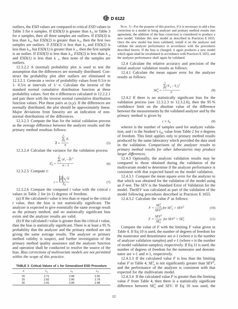
TABLE 3 Critical Values of l for Generalized ESD Procedure

n l1 l2 l3

20 2.71 2.68 2.6525 2.82 2.80 2.7830 2.91 2.89 2.88

D 6122

12

performance of the analyzer may be poorer than would beexpected on the basis of the model validation results. Conductfurther investigation of the analyzer function and operation toresolve the source of the poor performance. If Eq 11 was used,the performance of the analyzer may be better than would beexpected on the basis of the model validation results.

13. Periodic Validation by Plotting Control Charts of theDifferences Between Methods

13.1 If the analyzer passes the initial validation test de-scribed in 12.1, check the stability of the differences betweenthe analyzer and primary method using the control charts. Usethree types of control charts as described in Practice D 6299.

13.2 Individual Values Control Chart for the Differences:13.2.1 Establish the initial control limits for these charts by:13.2.1.1 Compute the differences,di, for the initial valida-

tion sample set of 20 using Eq 3.13.2.1.2 Compute the mean differenced (d-bar) and moving

rangeMR (MR-bar) as follows.

d 5(i51

n

di

n (12)

MR5(i51

n–1

?di11 – di?n – 1 (13)

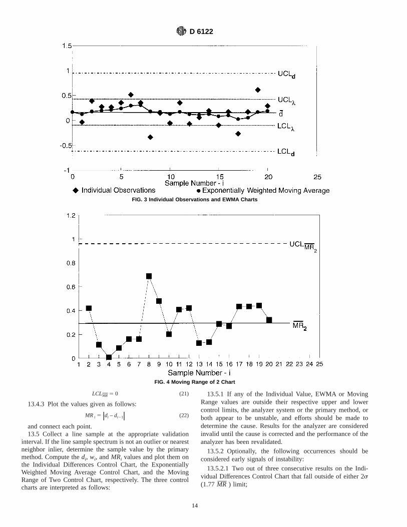
13.2.1.3 Construct the Individual Values Control Chart forthe differences as shown in Fig. 3 with the following controllimits.

UCLd 5 d 1 2.66 MR (14)

LCLd 5 d – 2.66MR (15)

13.2.2 Plot the differences,di, but do not connect the points.

13.3 Exponentially Weighted Moving Average (EWMA)Control Chart:

13.3.1 Overlay the Individual Values chart with an Expo-nentially Weighted Moving Average (EWMA) Control Chartfor the differences.(3)

13.3.2 Calculate the control limits for the ExponentiallyWeighted Moving Average chart using a weight (lambda) of0.2 to 0.4 as follows. See Fig. 3. A lambda value of 0.4 closelyemulates the run rule effects of conventional control charts,while a value of 0.2 has optimal prediction properties for thenext expected value. In addition, these lambda values alsoconveniently place the control limits (3-sigma) for the EWMAtrend at the 1-sigma (for 0.2 lambda) to 1.5-sigma (for 0.4lambda) values for the Individual Observations Chart.

UCLl 5 d 1 2.66MRŒ l2 –l (16)

LCL l 5 d 1 2.66 MRŒ l2 –l (17)

13.3.3 Calculate sequence values,wi, and plot them on theEWMA control chart.w0 is the initial value assumed fori 5 0in calculatingw 1 using the recursion Eq 19

w0 5 d (18)

wi 5 ~1 –l!wi21 1 ldi (19)

13.3.4 Plot thew i values on the chart and connect thepoints.

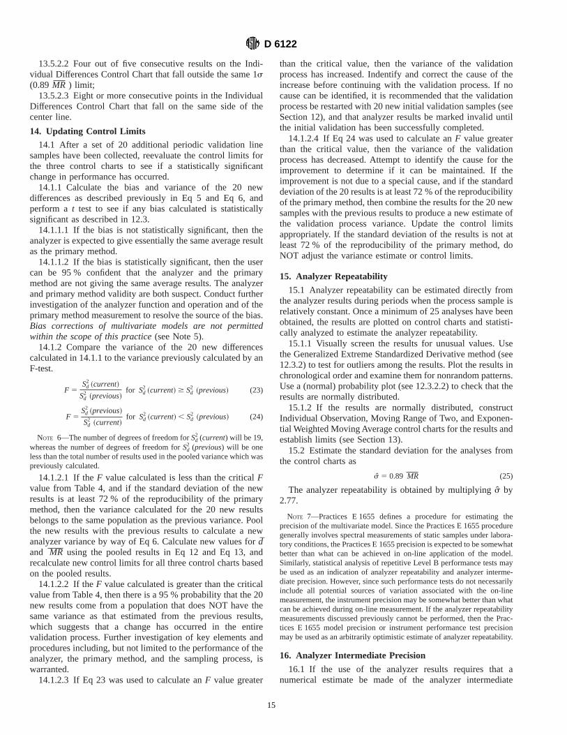
13.4 Moving Range of Two Control Chart:13.4.1 Construct a separate Moving Range of Two Control

Chart.13.4.2 See Fig. 4. The control limits are given as follows:

UCLMR 5 3.27MR (20)

TABLE 4 95 th Percentiles of the F- Distribution

Degrees of Freedom Numerator (Number of Analyzer Validation Samples)

Degrees

20 21 22 23 24 25 30

8 3.15 3.14 3.13 3.12 3.12 3.11 3.0812 2.54 2.53 2.52 2.51 2.51 2.50 2.4716 2.28 2.26 2.25 2.24 2.24 2.23 2.1920 2.12 2.11 2.10 2.09 2.08 2.07 2.0424 2.03 2.01 2.00 1.99 1.98 1.97 1.9428 1.96 1.95 1.93 1.92 1.91 1.91 1.87

of

32 1.91 1.90 1.88 1.87 1.86 1.85 1.8236 1.87 1.86 1.85 1.83 1.82 1.81 1.7840 1.84 1.83 1.81 1.80 1.79 1.78 1.74

Freedom

44 1.81 1.80 1.79 1.78 1.77 1.76 1.7248 1.79 1.78 1.77 1.76 1.75 1.74 1.7052 1.78 1.76 1.75 1.74 1.73 1.72 1.6856 1.76 1.75 1.74 1.72 1.71 1.70 1.6660 1.75 1.73 1.72 1.71 1.70 1.69 1.6564 1.74 1.72 1.71 1.70 1.69 1.68 1.6468 1.73 1.71 1.70 1.69 1.68 1.67 1.63

DenomInator

72 1.72 1.70 1.69 1.68 1.67 1.66 1.62

76 1.71 1.70 1.68 1.67 1.66 1.65 1.61

80 1.70 1.69 1.68 1.67 1.65 1.64 1.60

84 1.70 1.68 1.67 1.66 1.65 1.64 1.59

88 1.69 1.68 1.66 1.65 1.64 1.63 1.59

92 1.69 1.67 1.66 1.65 1.64 1.63 1.58

96 1.68 1.67 1.65 1.64 1.63 1.62 1.58

100 1.68 1.66 1.65 1.64 1.63 1.62 1.57

` 1.57 1.56 1.54 1.53 1.52 1.51 1.46

D 6122

13

LCLMR 5 0 (21)

13.4.3 Plot the values given as follows:

MRi 5?di – di21? (22)

and connect each point.13.5 Collect a line sample at the appropriate validation

interval. If the line sample spectrum is not an outlier or nearestneighbor inlier, determine the sample value by the primarymethod. Compute thedi, wi, andMRi values and plot them onthe Individual Differences Control Chart, the ExponentiallyWeighted Moving Average Control Chart, and the MovingRange of Two Control Chart, respectively. The three controlcharts are interpreted as follows:

13.5.1 If any of the Individual Value, EWMA or MovingRange values are outside their respective upper and lowercontrol limits, the analyzer system or the primary method, orboth appear to be unstable, and efforts should be made todetermine the cause. Results for the analyzer are consideredinvalid until the cause is corrected and the performance of theanalyzer has been revalidated.

13.5.2 Optionally, the following occurrences should beconsidered early signals of instability:

13.5.2.1 Two out of three consecutive results on the Indi-vidual Differences Control Chart that fall outside of either 2s(1.77MR ) limit;

FIG. 3 Individual Observations and EWMA Charts

FIG. 4 Moving Range of 2 Chart

D 6122

14

13.5.2.2 Four out of five consecutive results on the Indi-vidual Differences Control Chart that fall outside the same 1s(0.89MR ) limit;

13.5.2.3 Eight or more consecutive points in the IndividualDifferences Control Chart that fall on the same side of thecenter line.

14. Updating Control Limits

14.1 After a set of 20 additional periodic validation linesamples have been collected, reevaluate the control limits forthe three control charts to see if a statistically significantchange in performance has occurred.

14.1.1 Calculate the bias and variance of the 20 newdifferences as described previously in Eq 5 and Eq 6, andperform a t test to see if any bias calculated is statisticallysignificant as described in 12.3.

14.1.1.1 If the bias is not statistically significant, then theanalyzer is expected to give essentially the same average resultas the primary method.

14.1.1.2 If the bias is statistically significant, then the usercan be 95 % confident that the analyzer and the primarymethod are not giving the same average results. The analyzerand primary method validity are both suspect. Conduct furtherinvestigation of the analyzer function and operation and of theprimary method measurement to resolve the source of the bias.Bias corrections of multivariate models are not permittedwithin the scope of this practice(see Note 5).

14.1.2 Compare the variance of the 20 new differencescalculated in 14.1.1 to the variance previously calculated by anF-test.

F 5Sd

2 ~current!

Sd2 ~previous!

for Sd2 ~current! $ Sd

2 ~previous! (23)

F 5Sd

2 ~previous!

Sd2 ~current!

for Sd2 ~current! , Sd

2 ~previous! (24)

NOTE 6—The number of degrees of freedom forSd2 (current) will be 19,

whereas the number of degrees of freedom forSd2 (previous) will be one

less than the total number of results used in the pooled variance which waspreviously calculated.

14.1.2.1 If theF value calculated is less than the criticalFvalue from Table 4, and if the standard deviation of the newresults is at least 72 % of the reproducibility of the primarymethod, then the variance calculated for the 20 new resultsbelongs to the same population as the previous variance. Poolthe new results with the previous results to calculate a newanalyzer variance by way of Eq 6. Calculate new values fordand MR using the pooled results in Eq 12 and Eq 13, andrecalculate new control limits for all three control charts basedon the pooled results.

14.1.2.2 If theF value calculated is greater than the criticalvalue from Table 4, then there is a 95 % probability that the 20new results come from a population that does NOT have thesame variance as that estimated from the previous results,which suggests that a change has occurred in the entirevalidation process. Further investigation of key elements andprocedures including, but not limited to the performance of theanalyzer, the primary method, and the sampling process, iswarranted.

14.1.2.3 If Eq 23 was used to calculate anF value greater

than the critical value, then the variance of the validationprocess has increased. Indentify and correct the cause of theincrease before continuing with the validation process. If nocause can be identified, it is recommended that the validationprocess be restarted with 20 new initial validation samples (seeSection 12), and that analyzer results be marked invalid untilthe initial validation has been successfully completed.

14.1.2.4 If Eq 24 was used to calculate anF value greaterthan the critical value, then the variance of the validationprocess has decreased. Attempt to identify the cause for theimprovement to determine if it can be maintained. If theimprovement is not due to a special cause, and if the standarddeviation of the 20 results is at least 72 % of the reproducibilityof the primary method, then combine the results for the 20 newsamples with the previous results to produce a new estimate ofthe validation process variance. Update the control limitsappropriately. If the standard deviation of the results is not atleast 72 % of the reproducibility of the primary method, doNOT adjust the variance estimate or control limits.

15. Analyzer Repeatability

15.1 Analyzer repeatability can be estimated directly fromthe analyzer results during periods when the process sample isrelatively constant. Once a minimum of 25 analyses have beenobtained, the results are plotted on control charts and statisti-cally analyzed to estimate the analyzer repeatability.

15.1.1 Visually screen the results for unusual values. Usethe Generalized Extreme Standardized Derivative method (see12.3.2) to test for outliers among the results. Plot the results inchronological order and examine them for nonrandom patterns.Use a (normal) probability plot (see 12.3.2.2) to check that theresults are normally distributed.

15.1.2 If the results are normally distributed, constructIndividual Observation, Moving Range of Two, and Exponen-tial Weighted Moving Average control charts for the results andestablish limits (see Section 13).

15.2 Estimate the standard deviation for the analyses fromthe control charts as

s 5 0.89 MR (25)

The analyzer repeatability is obtained by multiplyings by2.77.

NOTE 7—Practices E 1655 defines a procedure for estimating theprecision of the multivariate model. Since the Practices E 1655 proceduregenerally involves spectral measurements of static samples under labora-tory conditions, the Practices E 1655 precision is expected to be somewhatbetter than what can be achieved in on-line application of the model.Similarly, statistical analysis of repetitive Level B performance tests maybe used as an indication of analyzer repeatability and analyzer interme-diate precision. However, since such performance tests do not necessarilyinclude all potential sources of variation associated with the on-linemeasurement, the instrument precision may be somewhat better than whatcan be achieved during on-line measurement. If the analyzer repeatabilitymeasurements discussed previously cannot be performed, then the Prac-tices E 1655 model precision or instrument performance test precisionmay be used as an arbitrarily optimistic estimate of analyzer repeatability.

16. Analyzer Intermediate Precision

16.1 If the use of the analyzer results requires that anumerical estimate be made of the analyzer intermediate

D 6122

15

precision (long-term analyzer stability), then it is recom-mended that this estimate be made from the repetitive analysesof a test sample whose spectrum is neither an outlier or anearest neighbor inlier. Conduct the analyses on a periodicbasis, no more frequently than once a day.

16.2 The conditions under which the test sample is analyzedshould mimic as closely as possible those used during routineanalyzer operation for analysis of line samples. Variableswhich shall be considered include, but are not limited to,sample temperature, flow rate, and pressure.

16.3 Once a minimum of 20 analyses have been obtained,plot the results on control charts and statistically analyze themto estimate the analyzer intermediate precision.

16.3.1 Visually screen the results for unusual values. Usethe Generalized Extreme Standardized Deviation Method (see12.3.2) to test for outliers among the results. Plot the results inchronological order and examine them for nonrandom patterns.Use a (normal) probability plot (see 12.3.2.2) to check that theresults are normally distributed.

16.3.2 Construct Individual Observation, Moving Range ofTwo, and Exponential Weighted Moving Average controlcharts for the results and establish limits (see Section 13).

16.4 Estimate the long-term standard deviation for theanalyses from the control charts as follows:

s 5 0.89MR (26)

The analyzer intermediate precision is obtained by multiply-ing s by 2.77.

16.5 Plot additional results from the precision test on the

control charts and update the limits each time an additional 20results are collected (see Section 14).

16.6 If the use of the analyzer results requires that theanalyzer intermediate precision estimate be continuously moni-tored over multiple test samples, then perform 20 analyses of anew test sample before the current test sample is depleted.Check thats2 for the new sample is statistically equivalent tothe s 2 obtained from previous test samples using theF-testdescribed in 14.1.2. Alternatively, a Q-chart(4) may be usedduring the initial change to the new test sample providing thereis a historical estimate of the analyzer intermediate precisionbased on at least 50 results.

NOTE 8—The analyzer intermediate precision calculated previously isonly an estimate of the true intermediate precision. How good the estimateis depends on a number of factors. The precision of the analyzer resultsmay vary across the multivariate space defined by the calibration model.A single test sample may not account for all this potential variation.Further, if the spectral measurement of the test sample is not done underconditions that are identical to those used during normal operation, themeasurement may not include some sources of variation and a lowestimate of the reproducibility may result. If the analyzer intermediateprecision is better that the analyzer repeatability (see Section 15), theintermediate precision estimate is probably not accounting for all sourcesof variation.

17. Keywords

17.1 control chart; infrared analyzer; infrared spectropho-tometers; IR spectroscopy; multivariate process; NIR spectros-copy; statistical quality assurance; validation

ANNEXES

(Mandatory Information)

A1. CONSIDERATIONS FOR QUANTITATIVE ON-LINE PROCESS IR MEASUREMENTS

A1.1 Spectral data collection and computation parametersused for the collection of process sample spectra shouldgenerally be identical to those used in collecting the calibrationspectra on which the multivariate model is based.

A1.1.1 The wavelength (frequency) range over which pro-cess sample spectra are collected shall be the same or greaterthan the range over which the calibration sample spectra werecollected. If the range is greater, the additional data collected isdiscarded prior to application of the model.

A1.1.2 The optical and digital resolution at which processsample spectra are collected should be identical to that used inthe collection of the calibration sample spectra.

A1.1.3 For instruments such as FT-IR where the spectra areobtained by mathematical processing of the raw spectral data,the processing conditions (for example, apodization, zero-filling, and so forth) employed in calculating the processsample spectra should be identical to those used in calculatingthe calibration sample spectra.

A1.1.4 Absorbances for the bands specified in this testmethod are expected to fall within the linear operating range ofthe spectrophotometer, as defined by the manufacturer, typi-

cally less than 1.0 absorbance units.A1.1.5 If the measurement time (for example, number of

averaged scans) is not the same for the process sample spectralmeasurement as for the measurement of the calibration samplespectra, then the user shall determine what effect this changehas on the precision of the analyzer results.

A1.2 Spectrophotometer Cells and Other InfraredSampling Methods

A1.2.1 One common process infrared measurement in-volves transmitting the infrared light through the sample whilethe sample is contained in a spectrophotometer cell. Thespectrophotometer cell consists of two infrared transparentwindows held apart at a fixed distance, the sample path length.The sample may flow through the cell during the spectralmeasurement, or the flow may be interrupted for the durationof the measurement.

A1.2.2 Inspect spectrophotometer cells and verify that thecells contribute minimally to the measured absorbance of thesample. If contamination or deposition on the cell windows issuspected, clean windows with an appropriate solvent, orreplace if necessary. Contamination can sometimes be detected

D 6122

16

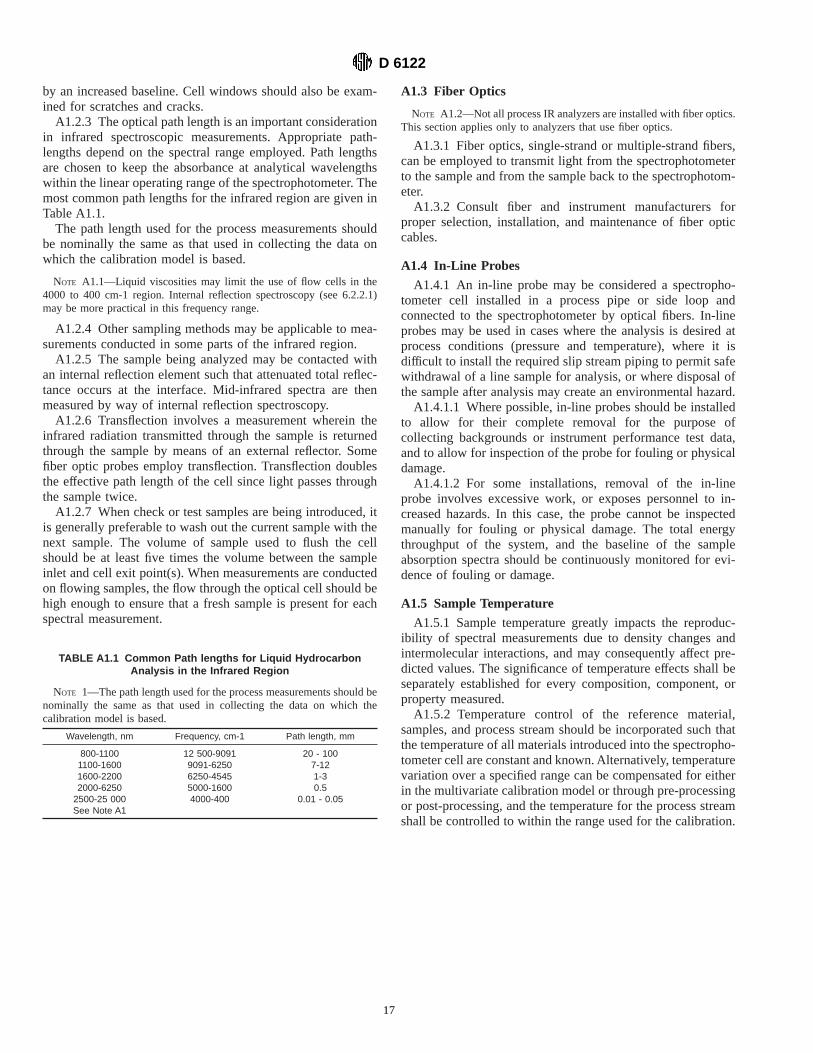
by an increased baseline. Cell windows should also be exam-ined for scratches and cracks.

A1.2.3 The optical path length is an important considerationin infrared spectroscopic measurements. Appropriate path-lengths depend on the spectral range employed. Path lengthsare chosen to keep the absorbance at analytical wavelengthswithin the linear operating range of the spectrophotometer. Themost common path lengths for the infrared region are given inTable A1.1.

The path length used for the process measurements shouldbe nominally the same as that used in collecting the data onwhich the calibration model is based.

NOTE A1.1—Liquid viscosities may limit the use of flow cells in the4000 to 400 cm-1 region. Internal reflection spectroscopy (see 6.2.2.1)may be more practical in this frequency range.

A1.2.4 Other sampling methods may be applicable to mea-surements conducted in some parts of the infrared region.

A1.2.5 The sample being analyzed may be contacted withan internal reflection element such that attenuated total reflec-tance occurs at the interface. Mid-infrared spectra are thenmeasured by way of internal reflection spectroscopy.

A1.2.6 Transflection involves a measurement wherein theinfrared radiation transmitted through the sample is returnedthrough the sample by means of an external reflector. Somefiber optic probes employ transflection. Transflection doublesthe effective path length of the cell since light passes throughthe sample twice.

A1.2.7 When check or test samples are being introduced, itis generally preferable to wash out the current sample with thenext sample. The volume of sample used to flush the cellshould be at least five times the volume between the sampleinlet and cell exit point(s). When measurements are conductedon flowing samples, the flow through the optical cell should behigh enough to ensure that a fresh sample is present for eachspectral measurement.

A1.3 Fiber Optics

NOTE A1.2—Not all process IR analyzers are installed with fiber optics.This section applies only to analyzers that use fiber optics.

A1.3.1 Fiber optics, single-strand or multiple-strand fibers,can be employed to transmit light from the spectrophotometerto the sample and from the sample back to the spectrophotom-eter.

A1.3.2 Consult fiber and instrument manufacturers forproper selection, installation, and maintenance of fiber opticcables.

A1.4 In-Line Probes

A1.4.1 An in-line probe may be considered a spectropho-tometer cell installed in a process pipe or side loop andconnected to the spectrophotometer by optical fibers. In-lineprobes may be used in cases where the analysis is desired atprocess conditions (pressure and temperature), where it isdifficult to install the required slip stream piping to permit safewithdrawal of a line sample for analysis, or where disposal ofthe sample after analysis may create an environmental hazard.

A1.4.1.1 Where possible, in-line probes should be installedto allow for their complete removal for the purpose ofcollecting backgrounds or instrument performance test data,and to allow for inspection of the probe for fouling or physicaldamage.

A1.4.1.2 For some installations, removal of the in-lineprobe involves excessive work, or exposes personnel to in-creased hazards. In this case, the probe cannot be inspectedmanually for fouling or physical damage. The total energythroughput of the system, and the baseline of the sampleabsorption spectra should be continuously monitored for evi-dence of fouling or damage.

A1.5 Sample Temperature

A1.5.1 Sample temperature greatly impacts the reproduc-ibility of spectral measurements due to density changes andintermolecular interactions, and may consequently affect pre-dicted values. The significance of temperature effects shall beseparately established for every composition, component, orproperty measured.

A1.5.2 Temperature control of the reference material,samples, and process stream should be incorporated such thatthe temperature of all materials introduced into the spectropho-tometer cell are constant and known. Alternatively, temperaturevariation over a specified range can be compensated for eitherin the multivariate calibration model or through pre-processingor post-processing, and the temperature for the process streamshall be controlled to within the range used for the calibration.

TABLE A1.1 Common Path lengths for Liquid HydrocarbonAnalysis in the Infrared Region

NOTE 1—The path length used for the process measurements should benominally the same as that used in collecting the data on which thecalibration model is based.

Wavelength, nm Frequency, cm-1 Path length, mm

800-1100 12 500-9091 20 - 1001100-1600 9091-6250 7-121600-2200 6250-4545 1-32000-6250 5000-1600 0.5

2500-25 000 4000-400 0.01 - 0.05See Note A1

D 6122

17

A2. INSTRUMENT PERFORMANCE TESTS

A2.1 Reference Materials for Instrument

A2.1.1 Check Samples—Check samples are generally usedfor conducting performance tests. Check samples are single,pure, liquid hydrocarbon compounds or mixtures of liquidhydrocarbon compounds of definite composition.

NOTE A2.1—If mixtures are utilized as check samples, they shall beprepared in a repeatable manner and, if stored, stored such that the mixtureis stable over long periods of time. In preparing mixtures of liquidhydrocarbon materials, components should be accurately pipetted orweighed at ambient temperature. It is recommended that mixtures beindependently verified for composition prior to use.

A2.1.1.1 The check sample is chosen such that its absorp-tion spectrum is similar to the petroleum matrix of theapplication of interest.

A2.1.1.2 When possible, the check sample should containthe major functional groups associated with the process streamof interest.

NOTE A2.2—The near-infrared spectral region is a simplified spectrumfor petroleum products in that the major bands are: aromatic, olefin,methyl, methylene, and oxygenates. For example, toluene is a frequentlychosen reference material for gasoline range petroleum products orintermediates. Toluene contains two major functional groups associatedwith gasoline, aromatic, and methyl functional groups.

A2.1.1.3 The check sample should have significant absor-bance at the wavelength(s) of interest. In order to adequatelydetermine the photometric linearity of the instrument, the peakabsorbance of a check sample should be similar to, andpreferably slightly greater than, the largest absorbance ex-pected from the process fluids.

A2.1.1.4 Mixtures can be used as check samples but theirspectra may be adversely affected by temperature-sensitiveinteractions that may manifest themselves by wavelength andabsorbance changes. Additionally, mixture composition maychange with time due to differential evaporation if samples arenot stored properly.

A2.1.2 Test Samples—A test sample is a process or productsample, or a mixture of process or product samples, whosespectrum is expected to be constant for the time period it isused in performance testing.

A2.1.2.1 Store the test sample in bulk quantities in con-trolled conditions such that the material is stable over time.

A2.1.2.2 Since test samples cannot be synthetically repro-duced, they can only be used for performance testing forlimited time periods. If test samples are used for this purpose,collection of historical data on a new test sample should beinitiated before previous test samples are depleted. It isrecommended that new test samples be analyzed sequentiallywith old test samples at least 15 times before they are used toreplace the old test sample. The 15 analyses shall be performedover a time period that does not exceed one month in duration.

A2.1.3 Optical Filters—An optical reference filter is anoptical filter or other optical device located in the spectropho-tometer or the sample probe which produces an absorptionspectrum which is known to be constant over time. This filtermay be automatically inserted into the optical path to allow

instrument performance tests to be performed.A2.1.3.1 Optical filters are used principally with in-line

probes when removal of the probe is inconvenient, precludingthe use of check or test samples for routine instrumentperformance testing.

A2.1.3.2 If an optical filter is used routinely to check orcorrect the spectral data collection or computation, then thesame filter cannot be used for instrument performance testing.For example, polystyrene filters are used to continuously checkand correct the wavelength scale of some dispersive NIRspectrophotometers. For such systems, polystyrene filtersshould not be employed for instrument performance testing.

A2.2 Types of Performance Tests

A2.2.1 Three types of performance tests are describedherein. ASTM Committee E-13 has defined Level 0 tests toconsist of a series of univariate instrument performance tests.The Level A and Level B tests defined herein are multivariateinstrument performance tests intended to be a rapid pass/failmeasure of the instrument performance.

A2.2.2 The Level 0, A, and B tests are intended to check thefollowing spectrophotometer variables: baseline, path length,wavelength, spectroscopic resolution, and photometric preci-sion and linearity.

A2.2.3 Level A tests involve the mathematical comparisonof the spectrum of a check or test sample against a historicalspectrum of the same material. Level B tests apply the actualprocess stream calibration model to analyze a check samplespectrum, a test sample spectrum, or the spectrum of an opticalfilter.

A2.2.4 Some Level 0 tests are specific for the type ofspectrophotometer in use (Fourier transform, diode array,monochromator, acousto-optic tunable filter, and so forth),whereas, Level A and Level B tests are applicable to allspectrophotometers. Level 0 tests for some specific instrumentshave been suggested or approved by Committee E-13. Teststhat might be useful in Level 0 procedures include thosediscussed in Practices E 275, E 932, E 1421 and E 1944.

A2.2.5 If the Level A or B test fails, it may be useful toperform a Level 0 test to provide diagnostics which mightpinpoint the cause of the failure.

A2.2.6 Level 0 and A tests can be developed prior to andutilized during and after the development of the processcalibration model. Although, by its very nature, the Level Btest can only be used after the process calibration model isdeveloped, it has the added advantage of providing someinformation about the sensitivity of the calibration model toinstrument performance parameters, especially when it isapplied to test samples rather than check samples or opticalfilters.

A2.2.7 Level 0 Tests:A2.2.7.1 Level 0 tests are not intended to provide absolute

measures of instrument performance, but rather useful diag-nostics that can be used to detect changes in instrumentperformance.

D 6122

18

A2.2.7.2 Level 0 tests measure various significant instru-ment parameters by specific univariate type measurementsperformed on the spectrum of a check sample, a test sample, oran optical filter. Parameters most frequently checked arewavelength precision, spectral resolution or bandwidth, base-line levels, photometric noise, and photometric linearity. All ofthe parameters measured should be plotted on control chartsand compared to historical values. The information derived isdirectly related to instrument performance and can be used fortrouble shooting.

A2.2.7.3 If Committee E-13 has not specified an appropriatetest procedure for the specific type of instrument used in theanalyzer, or if the sample specified by the Committee E-13procedure is incompatible with process operation, then thefollowing guidelines can be used to develop a practical Level0 test.

NOTE A2.3—A variety of algorithms can be used to calculate peakpositions, photometric noise, baseline stability, and resolution fromspectral data. Not all algorithms produce results of sufficient precision tobe useful for instrument performance testing. The calculations in thefollowing guidelines are intended as examples. The algorithms used incalculations of performance test results should be tested to demonstratethat they accurately track changes in instrument performance.

A2.2.7.4 A wavelength (or frequency) stability test is con-ducted by monitoring the positions of one or more absorbancepeaks for a check sample, a test sample or an optical filter. It isrecommended that the peak position be determined by thefollowing steps:

(a) Compute the first derivative of the spectrum by applyingthe appropriate digital filter to the spectrum. A commonly usedfilter has been defined by Savitzki and Golay(5) with correc-tions by Steiner, J., Termonia, Y., andDeltour, J.(6), withapplication criteria discussed by Willson and Polo(7). Thelatter reference discusses optimum filter parameters based uponthe relationship between spectral bandwidth and digitizationinterval.

(b) Identify the zero crossing associated with the peakabsorbance and compute its location by linear interpolationbetween the two adjacent points straddling the zero crossing.The zero crossing is taken as a measure of the peak position.

NOTE A2.4—The preceding test of wavelength stability can be affectedby photometric noise. To minimize the effect of noise, the peaks used forwavelength stability testing should be less than 1.0 absorbance, andpreferably below 0.7 absorbance.

A2.2.7.5 Photometric noise tests are conducted at two ormore spectral regions, preferably areas of minimum absor-bance. A spectral region used in the test covers at least elevenadjacent points. Two successive absorbance spectra of thecheck sample, the test sample, or the optical filter are collected.The second spectrum is subtracted from the first to generate adifference spectrum. The average value in each spectral regionis calculated for the difference spectrum and the standarddeviation about the average is calculated. The photometricnoise is the standard deviation about the average.

Photometric noise5Œ(i51

n

~Ai – A! 2

n – 1 (A2.1)

Ai is the absorbance value of the difference spectrum at the

i th data point,A is the average absorbance over then datapoints.

NOTE A2.5—The preceding measurement of photometric noise can beaffected by wavelength instability if there is a significant change inabsorbance across the region used in the noise calculation.

A2.2.7.6 Baseline stability is calculated for the same re-gions used in the photometric noise test. For a single spectrum,the mean absorbance for each region is computed and com-pared to historical data. Variation from the historical value istaken as an indication of baseline instability.

A2.2.7.7 Spectral resolution at one or more peaks in thespectrum of a check sample, a test sample, or an optical filtershould be monitored for stability. It is recommended that thespectral resolution of each peak be determined by the followingsteps.

(a) Compute the second derivative of the spectrum byapplying an appropriate digital filter to the spectrum. Acommonly used filter has been defined by Savitzki and Golay(5) with corrections by Steiner, J., Termonia, Y., and Deltour, J.(6), with application criteria discussed by Willson and Polo(7).The latter reference discusses optimum filter parameters basedupon the relationship between spectral bandwidth and digiti-zation interval.

(b) Identify the zero crossing on both sides of the minimumassociated with the peak absorbance and computing theirlocations by linear interpolation from the two adjacent pointsstraddling the zero crossing. The difference in the locations ofthe two zero crossings is taken as a measure of the spectralresolution.

NOTE A2.6—The preceding test of spectral resolution can be affectedby photometric noise.

A2.2.7.8 Photometric linearity is tested using two peaks inthe absorbance spectrum, one of which is the peak of maxi-mum absorbance. The second peak is preferably less than halfthe absorbance of the maximum peak. Linear baselines foreach peak are calculated from points of minimal absorbance onopposite sides of the peaks. The maximum absorbance for eachpeak is corrected for the baseline, and the ratio of theabsorbances for the two peaks is calculated. The ratio is usedto track changes in the photometric linearity.

NOTE A2.7—This test is sensitive to wavelength instabilities. A signifi-cant change in the ratio can be taken as evidence of a change inphotometric linearity, only if wavelength stability has been demonstrated.

A2.2.8 Level A Tests:A2.2.8.1 A Level A performance test is a pass/fail test that

is sensitive to all of the Level 0 parameters. Level A tests donot identify specific failure modes, but merely indicate if theinstrument performance is within historical bounds. In this test,the spectrum of a check sample, a test sample or an opticalfilter is compared to a historical spectra of the check sample,the test sample, or the optical filter by multivariate methods(least squares fitting or a PCR/PLS model). This procedure canprovide some information about specific instrument param-eters, but essentially looks for deviations in the residualspectrum as compared to the historical residual spectra. Thespectral range used in Level A tests should be comparable tothat used in the calibration model. If the spectrum of the check

D 6122

19

sample, the test sample, or the optical filter used in the LevelA test contains absorptions that are significantly higher thanthose of the calibration samples, then these peaks can beexcluded from the Level A fit.

A2.2.8.2 Level A Tests Using a Least Squares Method.—Ina Level A test, a least square fit of the current spectrum of thecheck sample, test sample, or optical filter is conducted againsta historical spectrum of the same material. Baseline terms maybe included in the fit to compensate for variations in baseline,and scaling may be applied to compensate for path lengthvariations. The types of compensations (baseline or pathlength) used in the fit should be similar to those employed inthe multivariate model used for the actual analyzer measure-ment. Methodology for calculating the least square fit isdiscussed by Blackburn, J.A.(8) and by Antoon, M.K., J.H.Koenig and J.L. Koenig(9). A typical least squares modelcould be

g 5 ah1 bl 1 c1 (A2.2)

whereg is the vector containing the current spectrum of thecheck sample, the test sample, or the optical filter,h is thevector containing the historical spectrum of the check sample,the test sample or the optical filter,l ( v for frequency basedspectra) is the vector of the wavelength axis values for spectrag andh, and 1 is a vector of ones.a is a coefficient for scalingthe historical spectrum to match the current spectrum.b is acoefficient which scalesl to provide a baseline correctionwhich is linear in wavelength (or frequency).c is a coefficientfor a baseline offset. The coefficientsa, b, and c are firstdetermined and then used to estimate the spectrum of thecurrent sample gˆ. The residuals from the fit are the differencebetween the measured and estimated values for the data points,g – g. The residuals from the fit are squared, and summed. Theresulting measure, herein referred to as the spectral residual, isused as a measure of changes in the instrument performance.This spectral residual should be plotted on control charts.Additionally, the scaling and baseline coefficients can bemonitored as an additional measure of instrument performance.

NOTE A2.8—Any function of the sum of the squares of the residualscan be used, for example, the square root.

A2.2.8.3 Level A Tests Using a PCR or PLS Method.—Toperform a Level A test using PCR or PLS, one shall firstdevelop an appropriate model. A series of historical spectra forthe check sample, the test sample or the optical filter areanalyzed without mean centering by a PCR or PLS regressionalgorithm using 100 % for the compositional value to generatethe Level A model. Generally, only one variable should beretained in the model since all the spectra are of the samematerial. The type of pre-processing or post-processing done inthe Level A test model should be comparable to that done in themultivariate calibration models being used on the analyzer. Theprincipal component or latent variable resulting from thismodel is applied to a current spectrum of the check sample, thetest sample, or the optical filter to generate a calculatedspectrum of the test sample, the check sample, or the opticalfilter. From this calculated spectrum, the spectral residual canbe computed as described previously. The spectral residual canbe charted to determine if the instrument is operating within

historical specifications.

NOTE A2.9—Chemometricians might refer to the analysis described inA2.2.8.3 as Principal Component Analysis rather than Principal Compo-nents Regression. However, the object here is to allow the Level A test tobe developed and applied using the same chemometric software employedin the development and application of the multivariate calibration model.

A2.2.9 Level B Tests:A2.2.9.1 A Level B performance test analyzes the spectrum

of a check sample, a test sample, or an optical filter against themodels in use on the analyzer system. As such, Level B testscan not be performed during calibration. Level B tests monitorthe instrument performance for deviations to which the cali-bration model is sensitive. Tests on a limited number ofsamples are not rigorous, but failure in these tests are indicativethat the analyzer operation has changed. The spectrum of thecheck sample, the test sample, or the optical filter is analyzedusing the multivariate model normally applied to line samples.The predicted value (property or component concentration),the Mahalanobis distance, and the spectral residuals are againcompared to historical values to detect any change in theanalyzer performance.

A2.3 Performance Test Charts

A2.3.1 Performance test results should be plotted on chartsand examined for trends. Such trend analysis may provideearly warnings of possible analyzer problems.

A2.3.2 Individual Value Control Charts, ExponentiallyWeighted Moving Average Control Charts, and Moving Rangeof Two Control Charts (see Section 13) can be used to detectstatistically significant changes in instrument performance.However, the statistical control limits associated with thesecharts will not necessarily be used to judge the performancetest results. Instead, some performance test results are typicallycompared to action limits as described in B5.

A2.3.3 For some performance tests, the test results areexpected to trend continuously in one direction until such timeas the analyzer is serviced. For example, the energy output ofan infrared source is expected to decrease continuously as thesource ages, until such time, as the source is cleaned orreplaced. The decreased energy may be observed as an increasein the Level 0 photometric noise, or as an increase in the LevelA spectral residual. The daily change in energy, noise, orresidual may be large relative to the precision with which thesevalues can be measured, but have tolerable effect on theaccuracy or precision of the analyzer results. For such tests,control charts and limits as discussed in Section 13 areinappropriate. An action limit for such tests needs to bedetermined from historical data or simulations as discussed inB5.

A2.3.4 For some performance tests, the test results areexpected to vary randomly about a fixed point. For example,for a properly operating instrument, the Level 0 wavelengthvalue might be expected to vary randomly about some averagevalue. For such tests, the control charts and control limitsdescribed in Section 13 can be usefully employed to set initialaction limits in the absence of historical data. Such initialaction limits may be loosened if statistically significant perfor-mance changes detected by the control charts are not found tohave significant effect on the validity of analyzer results.

D 6122

20

A2.3.5 Since Level B composition or property results forcheck or test samples are most directly comparable to actualanalyzer results, the Level B composition or property estimatesare most amenable to statistical control charting. Action limitsfor Level B composition or property estimates can be set to thecontrol limits described in Section 13.

A2.4 Performance Test Action Limits

A2.4.1 Calibration models differ greatly in their sensitivityto various aspects of instrument performance, and each appli-cation differs in what constitutes an acceptable tolerance tochanges in the results caused by variations in instrumentperformance. Although instrument performance tests are usefulin their own right, the process analyst should be concernedwith how changes in the instrument performance propagatethrough the calibration model and affect the calculated results.Historical databases or simulations that define acceptableperformance for one application may not be appropriate foranother application. In addition, the level of performancerequired by an application may be changed by the updating ofthe calibration model.

A2.4.2 Setting Action Limits Based on Historical Data forPerformance Tests:

A2.4.2.1 Performance tests provide measures of instrumentperformance. These measures can be compared to historicaldata for the same tests in order to judge the adequacy ofanalyzer performance. If historical data exist, limits for eachtest can be set and the performance can be judged against theselimits. If historical data do not exist, it will be necessary tocollect it as a standard part of the analyzer operation, and suchcollection will eventually allow performance limits to beestablished. The collection of the historical database forperformance tests is an integral part of the analyzer operation,and continues for the life of the analyzer.

A2.4.2.2 If the analyzer results for validation samples are inagreement with the results from the primary method, then theresults for the performance tests conducted during the sametime period should be considered an example of acceptableinstrument performance and added to the historical database.

A2.4.2.3 If the analyzer results are not in agreement withthe results from the primary method, and if the primary methodis within statistical quality control, the results from the perfor-mance tests may be examples of unacceptable instrumentperformance, particularly if the results from the performancetests are inconsistent with the historical database. Examples ofunacceptable instrument performance can be used to set actionlimits for future performance tests.

A2.4.2.4 It is strongly recommended that, at the time themultivariate model is developed, spectra of the check sample,the test sample, or the optical filter be collected along withspectra of the calibration and model validation samples.Performance tests can be applied to this data to determine thelevel of performance at the time of calibration. If a calibrationmodel was developed and validated, then the level of perfor-mance measured during the calibration period is adequate toproduce the precision demonstrated during calibration andvalidation of the model.

A2.4.2.5 Changes in analyzer performance that are detectedby Level 0 tests may or may not produce a significant change

in the results produced by the analyzer. Different types ofmultivariate models differ significantly in their sensitivity tovarious aspects of analyzer performance. By plotting the Level0 test results against analyzer results on control charts, condi-tions that lead to invalid analyzer results can be identified, andaction limits for each Level 0 test can eventually be estab-lished.

A2.4.2.6 Increases in the spectral residuals that are detectedby Level A tests will generally reflect some change in theresults produced by the analyzer. Even if the analyzer resultdoes not change, the spectral residuals measured as part of theoutlier testing will generally be expected to increase. The levelof increase that can be tolerated can be determined by plottingthe Level A test spectral residuals against analyzer results, anddetermining the maximum level at which valid analyzer resultsare produced.

A2.4.2.7 Changes in the values produced by a Level B testare the most straightforward to interpret since the values aredirectly comparable to the analyzer results. If the analysis ofthe spectrum of the check sample, the test sample, or theoptical filter is an interpolation of the model, then limits can beset directly based on the desired performance of the analyzer.If the analysis of the spectrum of the check sample, the testsample, or the optical filter is an extrapolation of the model,exercise care in setting limits since the extrapolated result maybe more sensitive to small changes in instrument performancethan analyses that are interpolations of the model. This isknown as leverage. In this case, initial limits should beconfirmed by plotting the Level B results against analyzerresults and determining the levels at which valid analyzerresults are produced.

NOTE A2.10—Any one test sample, check sample, or optical filter onlytests a small portion of the multivariate model space, and may not besensitive to all aspects of analyzer performance. The Level 0, A, and Btests are intended to detect possible analyzer failure modes. Acceptableperformance as measured by Level 0, A, and B tests is necessary but notsufficient by themselves for demonstrating valid analyzer performance.Comparison of analyzer results to in control, primary method laboratoryvalues is also necessary to demonstrate the validity of analyzer results.

A2.4.3 Determining Performance Action Limits by Simulat-ing Instrument Response Changes:

A2.4.3.1 An alternative procedure for determining actionlimits for instrument performance tests is to take actual,diverse, but representative spectra that are predicted well bythe model, and to mathematically modify these spectra tosimulate the expected variations in the instrument perfor-mance. The model sensitivity, for example, the change in theresults per unit change in a performance parameter, can beestimated and used to establish action limits for each perfor-mance parameter based on the error tolerance for the applica-tion. Instrument performance parameters which can be mod-eled include wavelength (frequency) shifts, baseline shifts,changes in photometric noise, resolution changes, and detectorlinearity changes. The importance of different performanceparameters is both application and instrument type dependent.Historical data for Level 0 performance tests are the best guideto the type of response changes that should be modeled for agiven instrument type.

A2.4.3.2 For example, the sensitivity of an analyzer to

D 6122

21

baseline drift can be simulated by adding various baselines toa set of representative spectra, analyzing these spectra with thecalibration model, and determining the change in the results asa function of the added baseline. The added baseline can, forexample, be parameterized in terms of offset, slope, andcurvature so that the effects of each can be determined.

A2.4.3.3 For example, the sensitivity of an analyzer towavelength (frequency) shift can be simulated by shifting thewavelength (frequency) of a set of representative spectra,analyzing these spectra with the calibration model, and deter-mining the change in the results as a function of the shift. If theshift is accomplished by way of interpolation of the spectra,exercise care that the interpolation function does not smooth orderesolve the spectra.

A2.4.3.4 Changes in instrument performance seldom affectonly one aspect of that performance. If simulations are used toset action limits for performance tests, it is essential thatmultiple performance parameters be varied simultaneously.The magnitude of the changes to the performance parametersthat should be simulated are best obtained from examination ofhistorical data on Level 0 performance tests conducted on thetype of instrument used in the analyzer.

A2.5 Tests for In-Line Probes

A2.5.1 Option A—Removal of the in-line probe from theprocess

A2.5.1.1 Whenever possible, it is preferable to remove thein-line probe from the process for the purpose of conducting aninstrument performance test.

A2.5.1.2 Removal of the in-line probe allows the entireoptical path to be examined during the performance test.Fouling or physical damage to the probe is more readilydetected.

A2.5.1.3 It will generally be necessary to clean the probebefore conducting instrument performance tests to remove anyresidual process sample which could contaminate the check ortest sample used in the tests. Similarly, it may be necessary toclean the probe after the tests if the check or test sample usedin the tests is incompatible with the process being measured.

A2.5.2 Option B—Temporarily disconnecting the in-lineprobe.

A2.5.2.1 For probes connected to the analyzer by opticalfibers, disconnect the fibers at the probe. Reconnect the fibersto an auxiliary probe, to a cuvette holder equipped withappropriate collimating optics or to a similar device. Collectthe spectrum of the check or test sample and continue with theLevel 0, A, or B test as described previously. Following thetests, reconnect the fibers to the in-line probe.

NOTE A2.11—If test samples are used for the instrument performancetests, it may be preferable to enclose the sample in a sealed cuvette toprevent differential evaporation of components and thus change in thechemical composition of the sample with time. Sealing these mixturesdoes not necessarily protect against thermal or photochemical degradationwhich can also alter chemical composition.

A2.5.2.2 When the in-line probe is not included in theoptical path during the instrument performance tests, theintegrity of the probe with respect to fouling and physicaldamage are not tested. Either of these two problems couldcontribute to invalid results.

A2.5.2.3 Fouling or contamination of the probe surface cansometimes be detected as changes in the baseline of the sampleabsorbance spectrum. The baseline should be monitored duringnormal operation for evidence of fouling.

A2.5.2.4 Physical damage to the probe could contribute toinvalid results. The total energy throughput of the opticalsystem should be monitored during normal operation forevidence of probe damage.

A2.5.3 Option C—Using a Reference Channel:A2.5.3.1 If the analyzer is equipped with multiple optical

channels, an alternative procedure is to dedicate one of theoptical channels as a reference channel for use in instrumentperformance tests. Level 0, A, or B tests are performed over thereference channel at the required interval.

A2.5.3.2 Performance tests conducted over a referencechannel do not test the entire optical path used for on-lineanalyses. While such tests may detect changes in source,spectrophotometer or detector performance, they are not af-fected by any changes in the fibers or probe in the on-linesample channel, nor are changes seen in the reference channelnecessarily mirrored in the other channels. It is the analyzervendor or user’s responsibility to demonstrate that performancemeasured on the reference channel is representative of perfor-mance on other channels.

A2.5.3.3 Energy throughput and sample absorbance spec-trum baseline should be monitored on each on-line channel forevidence of probe fouling or physical damage, or for changesin fiber tranmittance.

A2.5.4 Option D—Use of An Optical Reference Filter:A2.5.4.1 The spectrum of the optical reference filter is

obtained by first acquiring a spectrum of the current on-linesample, inserting the filter into the optical path, and collectinga spectrum of the filter (plus sample). The absorbance spectrumof the filter is calculated as follows:

Afilter 5 – log SSpectrumfilter 1 sample

SpectrumsampleD (A2.3)

Implicit to the successful use of this option is the assumptionthat the sample composition does not change significantly overthe time required to collect the two spectra. The spectra shouldbe collected as quickly as possible and in rapid succession.Testing should be performed during periods when the processis relatively stable to avoid compositional changes in thesample spectrum. Results of the tests using this option arecomparable only when the tests are run with identical spectralacquisition times.

A2.5.4.2 Level 0, A, or B tests are conducted on theabsorbance spectrum of the optical filter. Tests conducted inusing this option should be designed to avoid spectral rangeswhere the sample absorptions will be strong (>1.0 absorbance),since the absorbance spectrum of the filter may be excessivelynoisy in such regions.

A2.5.4.3 Option D will not detect fouling of the probe sincethe optical effects of such fouling will be present in both of thespectra ratioed in Annex A3. Performance tests conductedusing optical filters can be supplemented with baseline andphotometric noise tests done on on-line spectra. Such testsshould be performed in regions where the sample absorbance isknown to be minimal.

D 6122

22

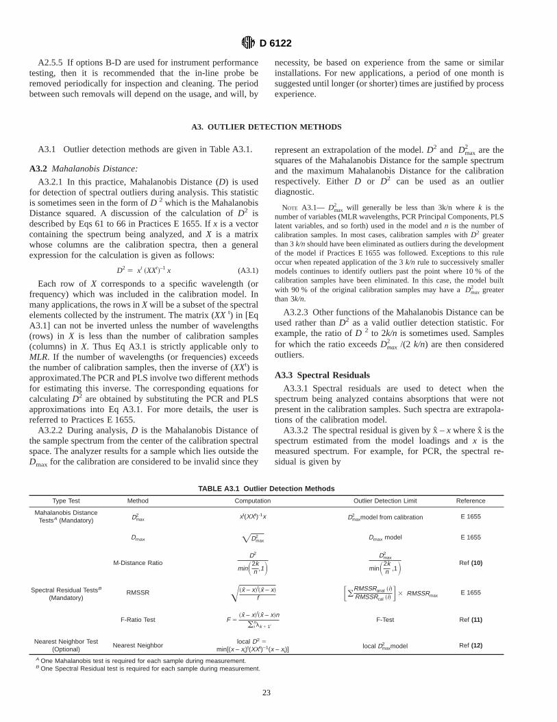
A2.5.5 If options B-D are used for instrument performancetesting, then it is recommended that the in-line probe beremoved periodically for inspection and cleaning. The periodbetween such removals will depend on the usage, and will, by

necessity, be based on experience from the same or similarinstallations. For new applications, a period of one month issuggested until longer (or shorter) times are justified by processexperience.

A3. OUTLIER DETECTION METHODS

A3.1 Outlier detection methods are given in Table A3.1.

A3.2 Mahalanobis Distance:

A3.2.1 In this practice, Mahalanobis Distance (D) is usedfor detection of spectral outliers during analysis. This statisticis sometimes seen in the form ofD 2 which is the MahalanobisDistance squared. A discussion of the calculation ofD2 isdescribed by Eqs 61 to 66 in Practices E 1655. Ifx is a vectorcontaining the spectrum being analyzed, andX is a matrixwhose columns are the calibration spectra, then a generalexpression for the calculation is given as follows:

D2 5 xt ~XXt!–1 x (A3.1)

Each row of X corresponds to a specific wavelength (orfrequency) which was included in the calibration model. Inmany applications, the rows inX will be a subset of the spectralelements collected by the instrument. The matrix (XX t) in [EqA3.1] can not be inverted unless the number of wavelengths(rows) in X is less than the number of calibration samples(columns) inX. Thus Eq A3.1 is strictly applicable only toMLR. If the number of wavelengths (or frequencies) exceedsthe number of calibration samples, then the inverse of (XXt) isapproximated.The PCR and PLS involve two different methodsfor estimating this inverse. The corresponding equations forcalculatingD2 are obtained by substituting the PCR and PLSapproximations into Eq A3.1. For more details, the user isreferred to Practices E 1655.

A3.2.2 During analysis,D is the Mahalanobis Distance ofthe sample spectrum from the center of the calibration spectralspace. The analyzer results for a sample which lies outside theDmax for the calibration are considered to be invalid since they

represent an extrapolation of the model.D2 and Dmax2 are the

squares of the Mahalanobis Distance for the sample spectrumand the maximum Mahalanobis Distance for the calibrationrespectively. EitherD or D2 can be used as an outlierdiagnostic.

NOTE A3.1— Dmax2 will generally be less than 3k/n wherek is the

number of variables (MLR wavelengths, PCR Principal Components, PLSlatent variables, and so forth) used in the model andn is the number ofcalibration samples. In most cases, calibration samples withD2 greaterthan 3k/nshould have been eliminated as outliers during the developmentof the model if Practices E 1655 was followed. Exceptions to this ruleoccur when repeated application of the 3k/n rule to successively smallermodels continues to identify outliers past the point where 10 % of thecalibration samples have been eliminated. In this case, the model builtwith 90 % of the original calibration samples may have aDmax

2 greaterthan 3k/n.

A3.2.3 Other functions of the Mahalanobis Distance can beused rather thanD2 as a valid outlier detection statistic. Forexample, the ratio ofD 2 to 2k/n is sometimes used. Samplesfor which the ratio exceedsDmax

2 /(2 k/n) are then consideredoutliers.

A3.3 Spectral Residuals

A3.3.1 Spectral residuals are used to detect when thespectrum being analyzed contains absorptions that were notpresent in the calibration samples. Such spectra are extrapola-tions of the calibration model.

A3.3.2 The spectral residual is given by xˆ – x where xis thespectrum estimated from the model loadings andx is themeasured spectrum. For example, for PCR, the spectral re-sidual is given by

TABLE A3.1 Outlier Detection Methods

Type Test Method Computation Outlier Detection Limit Reference

Mahalanobis DistanceTestsA (Mandatory) Dmax

2 xt(XXt)-1x Dmax2 model from calibration E 1655

Dmax =Dmax2 Dmax model E 1655

M-Distance RatioD2

minS2kn ,1D

Dmax2

minS2kn ,1D Ref (10)

Spectral Residual TestsB

(Mandatory)RMSSR Œ~x – x!t~x – x!

f F(RMSSRanal ~i!RMSSRcal ~i! G 3 RMSSRmax E 1655

F-Ratio Test F 5~x – x!t~x – x!n

(inlk 1 1i

F-Test Ref (11)

Nearest Neighbor Test(Optional)

Nearest Neighborlocal D2 5

min[(x – xi)t(XXt)–1(x – xi)]

local Dmax2 model Ref (12)

A One Mahalanobis test is required for each sample during measurement.B One Spectral Residual test is required for each sample during measurement.

D 6122

23

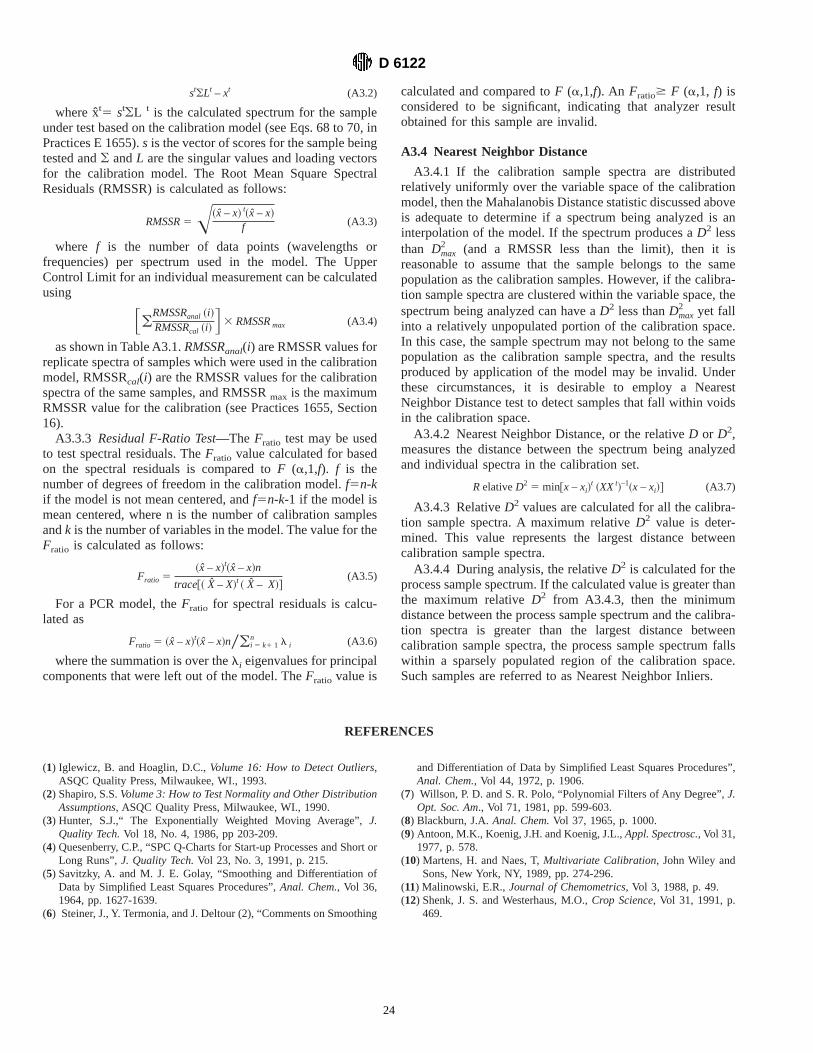
st(Lt – xt (A3.2)

where xt5 st(L t is the calculated spectrum for the sampleunder test based on the calibration model (see Eqs. 68 to 70, inPractices E 1655).s is the vector of scores for the sample beingtested and( andL are the singular values and loading vectorsfor the calibration model. The Root Mean Square SpectralResiduals (RMSSR) is calculated as follows:

RMSSR5Œ~x – x! t~x – x!f (A3.3)

where f is the number of data points (wavelengths orfrequencies) per spectrum used in the model. The UpperControl Limit for an individual measurement can be calculatedusing

F(RMSSRanal ~i!RMSSRcal ~i!

G3 RMSSRmax (A3.4)

as shown in Table A3.1.RMSSRanal(i) are RMSSR values forreplicate spectra of samples which were used in the calibrationmodel, RMSSRcal(i) are the RMSSR values for the calibrationspectra of the same samples, and RMSSRmax is the maximumRMSSR value for the calibration (see Practices 1655, Section16).

A3.3.3 Residual F-Ratio Test—The Fratio test may be usedto test spectral residuals. TheFratio value calculated for basedon the spectral residuals is compared toF (a,1,f). f is thenumber of degrees of freedom in the calibration model.f5n-kif the model is not mean centered, andf5n-k-1 if the model ismean centered, where n is the number of calibration samplesandk is the number of variables in the model. The value for theFratio is calculated as follows:

Fratio 5~x – x!t~x – x!n

trace@~ X – X!t ~ X – X!#(A3.5)

For a PCR model, theFratio for spectral residuals is calcu-lated as

Fratio 5 ~x – x!t~x – x!n/(i 5 k1 1n l i (A3.6)

where the summation is over theli eigenvalues for principalcomponents that were left out of the model. TheFratio value is

calculated and compared toF (a,1,f). An Fratio$ F (a,1, f) isconsidered to be significant, indicating that analyzer resultobtained for this sample are invalid.

A3.4 Nearest Neighbor Distance

A3.4.1 If the calibration sample spectra are distributedrelatively uniformly over the variable space of the calibrationmodel, then the Mahalanobis Distance statistic discussed aboveis adequate to determine if a spectrum being analyzed is aninterpolation of the model. If the spectrum produces aD2 lessthan Dmax

2 (and a RMSSR less than the limit), then it isreasonable to assume that the sample belongs to the samepopulation as the calibration samples. However, if the calibra-tion sample spectra are clustered within the variable space, thespectrum being analyzed can have aD2 less thanDmax

2 yet fallinto a relatively unpopulated portion of the calibration space.In this case, the sample spectrum may not belong to the samepopulation as the calibration sample spectra, and the resultsproduced by application of the model may be invalid. Underthese circumstances, it is desirable to employ a NearestNeighbor Distance test to detect samples that fall within voidsin the calibration space.

A3.4.2 Nearest Neighbor Distance, or the relativeD or D2,measures the distance between the spectrum being analyzedand individual spectra in the calibration set.

RelativeD2 5 min@x – xi!t ~XXt!–1~x – xi!# (A3.7)

A3.4.3 RelativeD2 values are calculated for all the calibra-tion sample spectra. A maximum relativeD2 value is deter-mined. This value represents the largest distance betweencalibration sample spectra.

A3.4.4 During analysis, the relativeD2 is calculated for theprocess sample spectrum. If the calculated value is greater thanthe maximum relativeD2 from A3.4.3, then the minimumdistance between the process sample spectrum and the calibra-tion spectra is greater than the largest distance betweencalibration sample spectra, the process sample spectrum fallswithin a sparsely populated region of the calibration space.Such samples are referred to as Nearest Neighbor Inliers.

REFERENCES

(1) Iglewicz, B. and Hoaglin, D.C.,Volume 16: How to Detect Outliers,ASQC Quality Press, Milwaukee, WI., 1993.

(2) Shapiro, S.S.Volume 3: How to Test Normality and Other DistributionAssumptions, ASQC Quality Press, Milwaukee, WI., 1990.

(3) Hunter, S.J.,“ The Exponentially Weighted Moving Average”,J.Quality Tech.Vol 18, No. 4, 1986, pp 203-209.

(4) Quesenberry, C.P., “SPC Q-Charts for Start-up Processes and Short orLong Runs”,J. Quality Tech.Vol 23, No. 3, 1991, p. 215.

(5) Savitzky, A. and M. J. E. Golay, “Smoothing and Differentiation ofData by Simplified Least Squares Procedures”,Anal. Chem., Vol 36,1964, pp. 1627-1639.

(6) Steiner, J., Y. Termonia, and J. Deltour (2), “Comments on Smoothing

and Differentiation of Data by Simplified Least Squares Procedures”,Anal. Chem., Vol 44, 1972, p. 1906.

(7) Willson, P. D. and S. R. Polo, “Polynomial Filters of Any Degree”,J.Opt. Soc. Am., Vol 71, 1981, pp. 599-603.

(8) Blackburn, J.A.Anal. Chem.Vol 37, 1965, p. 1000.(9) Antoon, M.K., Koenig, J.H. and Koenig, J.L.,Appl. Spectrosc., Vol 31,

1977, p. 578.(10) Martens, H. and Naes, T,Multivariate Calibration, John Wiley and

Sons, New York, NY, 1989, pp. 274-296.(11) Malinowski, E.R.,Journal of Chemometrics, Vol 3, 1988, p. 49.(12) Shenk, J. S. and Westerhaus, M.O.,Crop Science, Vol 31, 1991, p.

469.

D 6122

24

The American Society for Testing and Materials takes no position respecting the validity of any patent rights asserted in connectionwith any item mentioned in this standard. Users of this standard are expressly advised that determination of the validity of any suchpatent rights, and the risk of infringement of such rights, are entirely their own responsibility.

This standard is subject to revision at any time by the responsible technical committee and must be reviewed every five years andif not revised, either reapproved or withdrawn. Your comments are invited either for revision of this standard or for additional standardsand should be addressed to ASTM Headquarters. Your comments will receive careful consideration at a meeting of the responsibletechnical committee, which you may attend. If you feel that your comments have not received a fair hearing you should make yourviews known to the ASTM Committee on Standards, at the address shown below.

This standard is copyrighted by ASTM, 100 Barr Harbor Drive, PO Box C700, West Conshohocken, PA 19428-2959, United States.Individual reprints (single or multiple copies) of this standard may be obtained by contacting ASTM at the above address or at610-832-9585 (phone), 610-832-9555 (fax), or [email protected] (e-mail); or through the ASTM website (www.astm.org).

D 6122

25