NORTHWEST TRAINING RANGE COMPLEX EIS/OEIS FINAL (SEPTEMBER 2010) APPENDIX D MARINE MAMMAL MODELING i T TABLE OF CONTENTS D MARINE MAMMAL MODELING...................................................................................... D-1 D.1 BACKGROUND AND OVERVIEW .............................................................................................. D-1 D.1.1 METRICS FOR PHYSIOLOGICAL EFFECT THRESHOLDS ............................................. D-2 D.1.2 DERIVATION OF AN EFFECTS THRESHOLD BASED ON EFD ..................................... D-3 D.1.3 DERIVATION OF A BEHAVIORAL EFFECT THRESHOLD BASED ON SPL ................ D-4 D.2 ACOUSTIC SOURCES ................................................................................................................ D-6 D.2.1 SONARS ................................................................................................................................... D-6 D.2.2 EXPLOSIVES........................................................................................................................... D-7 D.3 ENVIRONMENTAL P ROVINCES ................................................................................................ D-9 D.3.1 IMPACT OF ENVIRONMENTAL PARAMETERS ............................................................ D-10 D.3.2 ENVIRONMENTAL PROVINCING METHODOLOGY .................................................... D-10 D.3.3 DESCRIPTION OF ENVIRONMENTAL PROVINCES ...................................................... D-11 D.4 I MPACT VOLUMES AND I MPACT RANGES ............................................................................ D-17 D.4.1 COMPUTING IMPACT VOLUMES FOR ACTIVE SONARS ........................................... D-18 D.4.1.1 Transmission Loss Calculations.......................................................................................... D-19 D.4.1.2 Energy Summation.............................................................................................................. D-19 D.4.1.3 Impact Volume per Hour of Sonar Operation ..................................................................... D-22 D.4.2 COMPUTING IMPACT VOLUMES FOR EXPLOSIVE SOURCES .................................. D-23 D.4.2.1 Transmission Loss Calculations.......................................................................................... D-23 D.4.2.2 Source Parameters ............................................................................................................... D-23 D.4.2.3 Impact Volumes for Various Metrics.................................................................................. D-25 D.4.2.4 Impact Volume per Explosive Detonation .......................................................................... D-27 D.4.3 IMPACT VOLUME BY REGION ......................................................................................... D-27 D.5 RISK F UNCTION:THEORETICAL AND P RACTICAL I MPLEMENTATION.............................. D-27 D.5.1 THRESHOLDS AND METRICS........................................................................................... D-28 D.5.2 MAXIMUM SOUND PRESSURE LEVEL ........................................................................... D-29 D.5.3 INTEGRATION ..................................................................................................................... D-29 D.5.3.1 Three Dimensions versus Two Dimensions........................................................................ D-31 D.5.4 THRESHOLD......................................................................................................................... D-31 D.5.5 MULTIPLE METRICS AND THRESHOLDS ...................................................................... D-32 D.5.6 CALCULATION OF EXPECTED EXPOSURES ................................................................. D-32 D.5.7 NUMERIC IMPLEMENTATION ......................................................................................... D-33 D.5.8 PRESERVING CALCULATIONS FOR FUTURE USE....................................................... D-34 D.5.9 SOFTWARE DETAIL............................................................................................................ D-35 D.6 EXPOSURE ESTIMATES .......................................................................................................... D-40 D.7 P OST ACOUSTIC MODELING ANALYSIS ............................................................................... D-41 D.7.1 MULTIPLE EXPOSURES IN GENERAL MODELING SCENARIO ................................. D-42 D.7.1.1 Solution to Ambiguity of Multiple Exposures in the General Modeling Scenario ............. D-42 D.7.1.2 Local Population: Upper Bound on Harassments ............................................................... D-44 D.7.1.3 Animal Motion Expansion .................................................................................................. D-44 D.7.1.4 Risk Function Expansion .................................................................................................... D-45 D.7.1.5 Example Case...................................................................................................................... D-47 D.7.2 LAND SHADOW ................................................................................................................... D-47 D.7.2.1 Computing the Land Shadow Effect at Each Grid Point .................................................... D-48 D.8 REFERENCES .......................................................................................................................... D-52

Welcome message from author
This document is posted to help you gain knowledge. Please leave a comment to let me know what you think about it! Share it to your friends and learn new things together.
Transcript

NORTHWEST TRAINING RANGE COMPLEX EIS/OEIS FINAL (SEPTEMBER 2010)
APPENDIX D MARINE MAMMAL MODELING i
TTABLE OF CONTENTS
D MARINE MAMMAL MODELING......................................................................................D-1
D.1 BACKGROUND AND OVERVIEW ..............................................................................................D-1D.1.1 METRICS FOR PHYSIOLOGICAL EFFECT THRESHOLDS .............................................D-2D.1.2 DERIVATION OF AN EFFECTS THRESHOLD BASED ON EFD .....................................D-3D.1.3 DERIVATION OF A BEHAVIORAL EFFECT THRESHOLD BASED ON SPL ................D-4D.2 ACOUSTIC SOURCES ................................................................................................................D-6D.2.1 SONARS...................................................................................................................................D-6D.2.2 EXPLOSIVES...........................................................................................................................D-7D.3 ENVIRONMENTAL PROVINCES................................................................................................D-9D.3.1 IMPACT OF ENVIRONMENTAL PARAMETERS ............................................................D-10D.3.2 ENVIRONMENTAL PROVINCING METHODOLOGY ....................................................D-10D.3.3 DESCRIPTION OF ENVIRONMENTAL PROVINCES......................................................D-11D.4 IMPACT VOLUMES AND IMPACT RANGES ............................................................................D-17D.4.1 COMPUTING IMPACT VOLUMES FOR ACTIVE SONARS ...........................................D-18D.4.1.1 Transmission Loss Calculations..........................................................................................D-19D.4.1.2 Energy Summation..............................................................................................................D-19D.4.1.3 Impact Volume per Hour of Sonar Operation.....................................................................D-22D.4.2 COMPUTING IMPACT VOLUMES FOR EXPLOSIVE SOURCES ..................................D-23D.4.2.1 Transmission Loss Calculations..........................................................................................D-23D.4.2.2 Source Parameters...............................................................................................................D-23D.4.2.3 Impact Volumes for Various Metrics..................................................................................D-25D.4.2.4 Impact Volume per Explosive Detonation..........................................................................D-27D.4.3 IMPACT VOLUME BY REGION.........................................................................................D-27D.5 RISK FUNCTION: THEORETICAL AND PRACTICAL IMPLEMENTATION..............................D-27D.5.1 THRESHOLDS AND METRICS...........................................................................................D-28D.5.2 MAXIMUM SOUND PRESSURE LEVEL...........................................................................D-29D.5.3 INTEGRATION .....................................................................................................................D-29D.5.3.1 Three Dimensions versus Two Dimensions........................................................................D-31D.5.4 THRESHOLD.........................................................................................................................D-31D.5.5 MULTIPLE METRICS AND THRESHOLDS......................................................................D-32D.5.6 CALCULATION OF EXPECTED EXPOSURES.................................................................D-32D.5.7 NUMERIC IMPLEMENTATION .........................................................................................D-33D.5.8 PRESERVING CALCULATIONS FOR FUTURE USE.......................................................D-34D.5.9 SOFTWARE DETAIL............................................................................................................D-35D.6 EXPOSURE ESTIMATES..........................................................................................................D-40D.7 POST ACOUSTIC MODELING ANALYSIS ...............................................................................D-41D.7.1 MULTIPLE EXPOSURES IN GENERAL MODELING SCENARIO.................................D-42D.7.1.1 Solution to Ambiguity of Multiple Exposures in the General Modeling Scenario .............D-42D.7.1.2 Local Population: Upper Bound on Harassments ...............................................................D-44D.7.1.3 Animal Motion Expansion..................................................................................................D-44D.7.1.4 Risk Function Expansion ....................................................................................................D-45D.7.1.5 Example Case......................................................................................................................D-47D.7.2 LAND SHADOW...................................................................................................................D-47D.7.2.1 Computing the Land Shadow Effect at Each Grid Point ....................................................D-48D.8 REFERENCES ..........................................................................................................................D-52

NORTHWEST TRAINING RANGE COMPLEX EIS/OEIS FINAL (SEPTEMBER 2010)
APPENDIX D MARINE MAMMAL MODELING ii
LLIST OF FIGURES
FIGURE D-1. SUMMER SVPS IN NWTRC................................................................................................................ D-13FIGURE D-2. WINTER SVPS IN NWTRC ................................................................................................................. D-13FIGURE D-3. NWTRC ENVIRONMENTAL PROVINCES OVER OPAREA ................................................................... D-16FIGURE D-4. HORIZONTAL PLANE OF VOLUMETRIC GRID FOR OMNI DIRECTIONAL SOURCE ................................. D-21FIGURE D-5. HORIZONTAL PLANE OF VOLUMETRIC GRID FOR STARBOARD BEAM SOURCE................................... D-21FIGURE D-6. 53C IMPACT VOLUME BY PING........................................................................................................... D-22FIGURE D-7. EXAMPLE OF AN IMPACT VOLUME VECTOR........................................................................................ D-22FIGURE D-8. 80-HZ BEAM PATTERNS ACROSS NEAR FIELD OF EER SOURCE ......................................................... D-25FIGURE D-9. 1250-HZ BEAM PATTERNS ACROSS NEAR FIELD OF EER SOURCE ..................................................... D-25FIGURE D-10. TIME SERIES ..................................................................................................................................... D-28FIGURE D-11. TIME SERIES SQUARED ..................................................................................................................... D-28FIGURE D-12. MAX SPL OF TIME SERIES SQUARED................................................................................................ D-29FIGURE D-13. PTS HEAVYSIDE THRESHOLD FUNCTION ......................................................................................... D-31FIGURE D-14. EXAMPLE OF A VOLUME HISTOGRAM............................................................................................... D-36FIGURE D-15. EXAMPLE OF THE DEPENDENCE OF IMPACT VOLUME ON DEPTH ...................................................... D-36FIGURE D-16. CHANGE OF IMPACT VOLUME AS A FUNCTION OF X-AXIS GRID SIZE ................................................ D-37FIGURE D-17. CHANGE OF IMPACT VOLUME AS A FUNCTION OF Y-AXIS GRID SIZE................................................ D-37FIGURE D-18. CHANGE OF IMPACT VOLUME AS A FUNCTION OF Y-AXIS GROWTH FACTOR.................................... D-38FIGURE D-19. CHANGE OF IMPACT VOLUME AS A FUNCTION OF BIN WIDTH.......................................................... D-38FIGURE D-20. DEPENDENCE OF IMPACT VOLUME ON THE NUMBER OF PINGS......................................................... D-39FIGURE D-21. EXAMPLE OF AN HOURLY IMPACT VOLUME VECTOR....................................................................... D-40FIGURE D-22. PROCESS OF CALCULATING H........................................................................................................... D-43FIGURE D-23. PROCESS OF SETTING AN UPPER BOUND ON INDIVIDUALS PRESENT IN AREA .................................. D-45FIGURE D-24. PROCESS OF EXPANDING AREA TO CREATE UPPER BOUND OF HARASSMENTS ................................ D-46FIGURE D-25. THE NEAREST POINT AT EACH AZIMUTH (WITH 1O SPACING) TO A SAMPLE GRID POINT (RED CIRCLE) IS
SHOWN BY THE GREEN LINES. ......................................................................................................................... D-48FIGURE D-26. APPROXIMATE PERCENTAGE OF BEHAVIORAL HARASSMENTS FOR EVERY 5 DEGREE BAND OF
RECEIVED LEVEL FROM THE 53C.................................................................................................................... D-49FIGURE D-27. AVERAGE PERCENTAGE OF HARASSMENTS OCCURRING WITHIN A GIVEN DISTANCE...................... D-50FIGURE D-28. DEPICTION OF LAND SHADOW OVER WARNING AREA 237............................................................... D-51FIGURE D-29. DEPICTION OF LAND SHADOW OVER NWTRC ................................................................................. D-51
LIST OF TABLES
TABLE D-1. HARASSMENT THRESHOLDS–EXPLOSIVES ............................................................................................. D-4TABLE D-2. ACTIVE SONARS EMPLOYED IN NWTRC............................................................................................... D-6TABLE D-3. REPRESENTATIVE SINKEX WEAPONS FIRING SEQUENCE..................................................................... D-9TABLE D-4. DISTRIBUTION OF BATHYMETRY PROVINCES IN NWTRC ................................................................... D-12TABLE D-5. DISTRIBUTION OF SVP PROVINCES IN NWTRC................................................................................... D-13TABLE D-6. DISTRIBUTION OF HIGH-FREQUENCY BOTTOM LOSS CLASSES IN NWTRC......................................... D-14TABLE D-7. DISTRIBUTION OF ENVIRONMENTAL PROVINCES IN GENERAL OPAREA OF NWTRC ........................ D-15TABLE D-8. DISTRIBUTION OF ENVIRONMENTAL PROVINCES WITHIN SINKEX AREA ........................................... D-17TABLE D-9. DISTRIBUTION OF ENVIRONMENTAL PROVINCES WITHIN W-237 ......................................................... D-17TABLE D-10. TL DEPTH AND RANGE SAMPLING PARAMETERS BY SONAR TYPE.................................................... D-19TABLE D-11. UNKNOWNS AND ASSUMPTIONS ........................................................................................................ D-41TABLE D-12. BEHAVIORAL HARASSMENTS AT EACH RECEIVED LEVEL BAND FROM 53C ...................................... D-49

NORTHWEST TRAINING RANGE COMPLEX EIS/OEIS FINAL (SEPTEMBER 2010)
APPENDIX D MARINE MAMMAL MODELING D-1
DD MARINE MAMMAL MODELINGD.1 BACKGROUND AND OVERVIEW
All marine mammals are protected under the Marine Mammal Protection Act (MMPA). The MMPA prohibits, with certain exceptions, the unauthorized take of marine mammals in U.S. waters and by U.S. citizens on the high seas, and the importation of marine mammals and marine mammal products into the United States.
The Endangered Species Act of 1973 (ESA) provides for the conservation of species that are endangered or threatened throughout all or a significant portion of their range, and the conservation of their ecosystems. A species is considered endangered if it is in danger of extinction throughout all or a significant portion of its range. A species is considered threatened if it is likely to become an endangered species within the foreseeable future. There are marine mammals, already protected under MMPA, listed as either endangered or threatened under ESA, and afforded special protections.
Actions involving sound in the water include the potential to harass marine animals in the surrounding waters. Demonstration of compliance with MMPA and the ESA, using best available science, has been assessed using criteria and thresholds accepted or negotiated, and described here.
Sections of the MMPA (16 United States Code [U.S.C.] 1361 et seq.) direct the Secretary of Commerce to allow, upon request, the incidental, but not intentional, taking of small numbers of marine mammals by U.S. citizens who engage in a specified activity, other than commercial fishing, within a specified geographical region. Through a specific process, if certain findings are made and regulations are issued, notice of a proposed authorization is provided to the public for review.
Authorization for incidental takings may be granted if the National Marine Fisheries Service (NMFS) finds that the taking will have no more than a negligible impact on the species or stock(s), will not have an immitigable adverse impact on the availability of the species or stock(s) for subsistence uses, and that the permissible methods of taking, and requirements pertaining to the mitigation, monitoring and reporting of such taking are set forth.
NMFS has defined negligible impact in 50 Code of Federal Regulations (CFR) 216.103 as an impact resulting from the specified activity that cannot be reasonably expected to, and is not reasonably likely to,adversely affect the species or stock through effects on annual rates of recruitment or survival.
Subsection 101(a)(5)(D) of the MMPA established an expedited process by which citizens of the United States can apply for an authorization to incidentally take small numbers of marine mammals by harassment. The National Defense Authorization Act of 2004 (NDAA) (Public Law 108-136) removed the small numbers limitation and amended the definition of “harassment” as it applies to a military readiness activity to read as follows:
(i) any act that injures or has the significant potential to injure a marine mammal or marine mammal stock in the wild [Level A Harassment]; or (ii) any act that disturbs or is likely to disturb a marine mammal or marine mammal stock in the wild by causing disruption of natural behavioral patterns, including, but not limited to, migration, surfacing, nursing, breeding, feeding, or sheltering, to a point where such behavioral patterns are abandoned or significantly altered [Level B Harassment].
The primary potential impact to marine mammals from underwater acoustics is Level B harassment from noise. For explosions of ordnance planned for use in the Northwest Training Range Complex (NWTRC), in the absence of any mitigation or monitoring measures, there is a very small chance that a marine mammal could be injured or killed when exposed to the energy generated from an explosive force.

NORTHWEST TRAINING RANGE COMPLEX EIS/OEIS FINAL (SEPTEMBER 2010)
APPENDIX D MARINE MAMMAL MODELING D-2
Analysis of noise impacts is based on criteria and thresholds initially presented in U.S. Navy Environmental Impact Statements (EISs) for ship shock trials of the Seawolf submarine and the Winston Churchill (DDG 81), in EISs for the Southern California and Hawaii Range Complexes, and subsequently adopted by NMFS.
Non-lethal injurious impacts (Level A Harassment) are defined in those documents as tympanic membrane (TM) rupture and the onset of slight lung injury. The threshold for Level A Harassment corresponds to a 50-percent rate of TM rupture, which can be stated in terms of an energy flux density (EFD) value of 205 decibels (dB) re 1 micro Pascal squared–second (μPa2-s). TM rupture is well-correlated with permanent hearing impairment. Ketten (1998) indicates a 30-percent incidence of permanent threshold shift (PTS) at the same threshold.
The criteria for onset of slight lung injury were established using partial impulse because the impulse of an underwater blast wave was the parameter that governed damage during a study using mammals, not peak pressure or energy (Yelverton, 1981). Goertner (1982) determined a way to calculate impulse values for injury at greater depths, known as the Goertner “modified” impulse pressure. Those values are valid only near the surface because as hydrostatic pressure increases with depth, organs like the lung, filled with air, compress. Therefore the “modified” impulse pressure thresholds vary from the shallow depth starting point as a function of depth.
The shallow depth starting points for calculation of the “modified” impulse pressures are mass-dependent values derived from empirical data for underwater blast injury (Yelverton, 1981). During the calculations, the lowest impulse and body mass for which slight, and then extensive, lung injury found during a previous study (Yelverton et al., 1973) were used to determine the positive impulse that may cause lung injury. The Goertner model is sensitive to mammal weight such that smaller masses have lower thresholds for positive impulse so injury and harassment will be predicted at greater distances from the source for them. Impulse thresholds of 13.0 and 31.0 pounds per square inch-millisecond (psi-msec), found to cause slight and extensive injury in a dolphin calf, were used as thresholds in the analysis contained in this document.
D.1.1 Metrics for Physiological Effect ThresholdsEffect thresholds used for acoustic impact modeling in this document are expressed in terms of EFD / Sound Exposure Level (SEL), which is total energy received over time in an area, or in terms of Sound Pressure Level (SPL), which is the level (root mean square) without reference to any time component for the exposure at that level. Marine and terrestrial mammal data show that, for continuous-type sounds of interest, Temporary Threshold Shift (TTS) and PTS are more closely related to the energy in the sound exposure than to the exposure SPL.
The Energy Level (EL) for each individual ping is calculated from the following equation:
EL = SPL + 10log10(duration)
The EL includes both the ping SPL and duration. Longer-duration pings and/or higher-SPL pings will have a higher EL.
If an animal is exposed to multiple pings, the EFD in each individual ping is summed to calculate the total EL. Since mammalian Threshold Shift (TS) data show less effect from intermittent exposures compared to continuous exposures with the same energy (Ward, 1997), basing the effect thresholds on the total received EL is a conservative approach for treating multiple pings; in reality, some recovery will occur between pings and lessen the effect of a particular exposure. Therefore, estimates are conservative because recovery is not taken into account (given that generally applicable recovery times have not been

NORTHWEST TRAINING RANGE COMPLEX EIS/OEIS FINAL (SEPTEMBER 2010)
APPENDIX D MARINE MAMMAL MODELING D-3
experimentally established) and as a result, intermittent exposures from sonar are modeled as if they were continuous exposures.
The total EL depends on the SPL, duration, and number of pings received. The TTS and PTS thresholds do not imply any specific SPL, duration, or number of pings. The SPL and duration of each received ping are used to calculate the total EL and determine whether the received EL meets or exceeds the effect thresholds. For example, the TTS threshold would be reached through any of the following exposures:
• A single ping with SPL = 195 dB re 1 μPa and duration = 1 second.
• A single ping with SPL = 192 dB re 1 μPa and duration = 2 seconds.
• Two pings with SPL = 192 dB re 1 μPa and duration = 1 second.
• Two pings with SPL = 189 dB re 1 μPa and duration = 2 seconds.D.1.2 Derivation of an Effects Threshold Based on EFDAs described in detail in Section 3.9.2.1 of the NWTRC EIS, SEL (EFD level) exposure threshold established for onset-TTS is 195 dB re 1 μPa2-s. This result is corroborated by the short-duration tone data of Finneran et al. (2000, 2003) and the long-duration sound data from Nachtigall et al. (2003a, b). Together, these data demonstrate that TTS in small odontocetes is correlated with the received EL and that onset-TTS exposures are fit well by an equal-energy line passing through 195 dB re 1 μPa2-s. Absent any additional data for other species and being that it is likely that small odontocetes are more sensitive to the mid-frequency active/high-frequency active (MFA/HFA) frequency levels of concern, this threshold is used for analysis for all cetacea.
The PTS thresholds established for use in this analysis are based on a 20 dB increase in exposure EL over that required for onset-TTS. The 20 dB value is based on estimates from terrestrial mammal data of PTS occurring at 40 dB or more of TS, and on TS growth occurring at a rate of 1.6 dB/dB increase in exposure EL. This is conservative because: (1) 40 dB of TS is actually an upper limit for TTS used to approximate onset-PTS, and (2) the 1.6 dB/dB growth rate is the highest observed in the data from Ward et al. (1958, 1959). Using this estimation method (20 dB up from onset-TTS) for the NWTRC analysis, the PTS threshold for cetacea is 215 dB re 1μPa2-s.
The threshold levels for analyzing acoustic impacts to pinnipeds from MFA/HFA sonar are based on specific species data when available. For the Stellar sea lion and Northern fur seal, the California sea lion data was used. Morphologically, the Stellar sea lion, Northern fur seal, and California sea lion are related. They are "eared" seals (Family Otarridae w/external ear flaps), vice the true seals (Family Phocidae w/out external ear flaps) such as harbor seals. In addition, the habitats and natural history (foraging, breeding, etc) are similar between Stellar sea lion, Northern fur seal, and California sea lion. The threshold levels for pinnipeds are given below:
Level A Harassment (onset PTS)
• Stellar Sea Lion 226 dB re 1 μPa2 ·s
• Northern Fur Seal 226 dB re 1 μPa2 ·s
• California Sea Lion 226 dB re 1 μPa2 ·s
• Northern Elephant Seal 224 dB re 1 μPa2 ·s
• Harbor Seal 203 dB re 1 μPa2 ·s
Level B Harassment (onset TTS)
• Stellar Sea Lion 206 dB re 1 μPa2 ·s

NORTHWEST TRAINING RANGE COMPLEX EIS/OEIS FINAL (SEPTEMBER 2010)
APPENDIX D MARINE MAMMAL MODELING D-4
• Northern Fur Seal 206 dB re 1 μPa2 ·s
• California Sea Lion 206 dB re 1 μPa2 ·s
• Northern Elephant Seal 204 dB re 1 μPa2 ·s
• Harbor Seal 183 dB re 1 μPa2 ·s
Level B (non-injurious) Harassment also includes a TTS threshold consisting of 182 dB maximum EFD level in any 1/3-octave band above 100 hertz (Hz) for toothed whales (e.g., dolphins). A second criterion, 23 psi, has recently been established by NMFS to provide a more conservative range for TTS when the explosive or animal approaches the sea surface, in which case explosive energy is reduced, but the peak pressure of 1 μPa2-s is not (Table D-1). NMFS applies the more conservative of these two.
There may be rare occasions when multiple successive explosions (MSE) are part of a static location event such as during Bombing Exercise (BOMBEX), Sinking Exercise (SINKEX), or Gunnery Exercise (GUNEX) (when using other than inert weapons). For MSEs, accumulated energy over the entire training time, not to exceed 24 hours, is the natural extension for energy thresholds since energy accumulates with each subsequent shot; this is consistent with the treatment of multiple arrivals in Churchill. For positive impulse, it is consistent with Churchill to use the maximum value over all impulses received.
For MSEs, the acoustic criterion for sub-TTS behavioral disturbance is used to account for behavioral effects significant enough to be judged as harassment, but occurring at lower sound energy levels than those that may cause TTS. The sub-TTS threshold is derived following the approach of the Churchill Final Environmental Impact Statement (FEIS) for the energy-based TTS threshold. The research on pure-tone exposures reported in Schlundt et al. (2000) and Finneran and Schlundt (2004) provided a threshold of 192 dB re 1 μPa2-s as the lowest TTS value. This value for pure-tone exposures is modified for explosives by (a) interpreting it as an energy metric, (b) reducing it by 10 dB to account for the time constant of the mammal ear, and (c) measuring the energy in 1/3 octave bands, the natural filter band of the ear. The resulting TTS threshold for explosives is 182 dB re 1 μPa2-s in any 1/3 octave band. As reported by Schlundt et al. (2000) and Finneran and Schlundt (2004), instances of altered behavior in the pure-tone research generally began five dB lower than those causing TTS. The sub-TTS threshold is therefore derived by subtracting 5 dB from the 182 dB re 1 μPa2-s in any 1/3 octave band threshold, resulting in a 177 dB re 1 μPa2-s (EL) sub-TTS behavioral disturbance threshold for MSE. Table D-1 lists the harassment thresholds for explosives.
TTable D-1. Haras s m ent Thres ho lds –Explos ives
Threshold Type (Explosives) Threshold Level
Sub-TTS Threshold for Multiple Successive Explosions (peak one-third octave energy)
177 dB
Level B - Temporary Threshold Shift (TTS) (peak one-third octave energy) 182 dB
Level B - Temporary Threshold Shift (TTS) (peak pressure) 23 psi
Level A – Slight lung injury (positive impulse) 13 psi-ms
Level A – 50% Eardrum rupture (peak one-third octave energy) 205 dB
Mortality – 1% Mortal lung injury (positive impulse) 31 psi-ms
D.1.3 Derivation of a Behavioral Effect Threshold Based on SPLOver the past several years, the Navy and NMFS have worked on developing alternative criteria to replace and/or to supplement the acoustic thresholds used in the past to estimate the probability of marine

NORTHWEST TRAINING RANGE COMPLEX EIS/OEIS FINAL (SEPTEMBER 2010)
APPENDIX D MARINE MAMMAL MODELING D-5
mammals being behaviorally harassed by received levels of MFA and HFA sonar. The Navy continues working with the NMFS to refine a mathematically representative curve for assessment of behavioral effects modeling associated with the use of MFA/HFA sonar. As detailed in Section 3.9.2.1.8, the NMFS Office of Protected Resources made the decision to use a risk function and applicable input parameters to estimate the probability of behavioral responses that NMFS would classify as harassment for the purposes of the MMPA given exposure to specific received levels of MFA/HFA sonar. This decision was based on the recommendation of the two NMFS scientists, consideration of the independent reviews from six scientists, and NMFS MMPA regulations affecting the Navy’s use of Surveillance Towed Array Sensor System Low-Frequency Active (SURTASS LFA) sonar (DoN, 2002; National Oceanic and Atmospheric Administration [NOAA], 2007).
The particular acoustic risk function developed by the Navy and NMFS is derived from a solution in Feller (1968) with input parameters modified by NMFS for MFA/HFA sonar for mysticetes, odontocetes, and pinnipeds. In order to represent a probability of risk in developing this function, the function would have a value near zero at very low exposures, and a value near one for very high exposures. One class of functions that satisfies this criterion is cumulative probability distributions, a type of cumulative distribution function. In selecting a particular functional expression for risk, several criteria were identified:
• The function must use parameters to focus discussion on areas of uncertainty;
• The function should contain a limited number of parameters;
• The function should be capable of accurately fitting experimental data; and
• The function should be reasonably convenient for algebraic manipulations.
As described in DoN 2001, the mathematical function below is adapted from a solution in Feller (1968).
A
A
KBL
KBL
R 2
1
1
−
−
⎟⎠⎞
⎜⎝⎛ −
−
⎟⎠⎞
⎜⎝⎛ −
−=
Where: R = risk (0 – 1.0);
L = Received Level (RL) in dB
B = basement RL in dB (120 dB)
K = the RL increment above basement in dB at which there is 50% risk
A = risk transition sharpness parameter (8 for mysticetes, 10 for all others)
It is important to note that the probabilities associated with acoustic modeling do not represent an individual’s probability of responding; they identify the proportion of an exposed population (as represented by an evenly distributed density of marine mammals per unit area) that is likely to respond to an exposure. In addition, modeling does not take into account reductions from any of the Navy’s standard protective mitigation measures which should significantly reduce or eliminate actual exposures that may have otherwise occurred during training.

NORTHWEST TRAINING RANGE COMPLEX EIS/OEIS FINAL (SEPTEMBER 2010)
APPENDIX D MARINE MAMMAL MODELING D-6
DD.2 ACOUSTIC S OURCES
The acoustic sources employed in the NWTRC are categorized as either broadband (producing sound over a wide frequency band) or narrowband (producing sound over a frequency band that that is small in comparison to the center frequency). In general, the narrowband sources in this exercise are Anti-Submarine Warfare (ASW) sonars and the broadband sources are explosives. This delineation of source types has a couple of implications. First, the transmission loss used to determine the impact ranges of narrowband ASW sonars can be adequately characterized by model estimates at a single frequency.Broadband explosives, on the other hand, produce significant acoustic energy across several frequency decades of bandwidth. Propagation loss is sufficiently sensitive to frequency as to require model estimates at several frequencies over such a wide band.
Second, the types of sources have different sets of harassment metrics and thresholds. Energy metrics are defined for both types. However, explosives are impulsive sources that produce a shock wave that dictates additional pressure-related metrics (peak pressure and positive impulse). Detailed descriptions of both types of sources are provided in the following subsections.
D.2.1 SonarsOperations in the NWTRC involve five types of narrowband sonars. Harassment estimates are calculated for each sonar according to the manner in which it operates. For example, the SQS-53C is a hull-mounted, surface ship sonar that operates for many hours at a time, so it is useful to calculate and report SQS-53C harassments per hour of operation. The AN/SSQ-62 is a sonobuoy that is dropped into the water from an aircraft or helicopter and pings about 10 to 30 times in an hour. For the AN/SSQ-62, it is most helpful to calculate and report exposures per sonobuoy. For the MK-48 torpedo, the sonar is modeled for a typical training event and the MK-48 reporting metric is the number of torpedo runs. Table D-2 presents the deploying platform, frequency class, and the reporting metrics for each narrow-band sonar used in the NWTRC.
Table D-2. Active Sona rs Emplo yed in NWTRC
Sonar Description Frequency Class Exposures Reported Units per Hour
MK-48 Torpedo sonar High-frequency Per torpedo One torpedo runAN/SQS-53C Surface ship sonar Mid-frequency Per hour 120 sonar pingsAN/SQS-56 Surface ship sonar Mid-frequency Per hour 120 sonar pingsAN/SSQ-62 Sonobuoy sonar Mid-frequency Per sonobuoy 8 sonobuoysAN/SSQ-125 Sonobuoy sonar Mid-frequency Per sonobuoy UnknownAN/BQS-15 Submarine sonar High-frequency Per hour Varies
Note that MK-48 source described here is the active pinger on the torpedo; the explosive source of the detonating torpedo is described in the next subsection.
The acoustic modeling that is necessary to support the harassment estimates for each of these sonars relies on a generalized description of the manner of the sonar’s operating modes. This description includes the following:
• “Effective” energy source level—This is the level relative to 1 μPa2-s of the integral over frequency and time of the square of the pressure and is given by the total energy level across the band of the source, scaled by the pulse length (10 log10 [pulse length]).
• Source depth—Depth of the source in meters.

NORTHWEST TRAINING RANGE COMPLEX EIS/OEIS FINAL (SEPTEMBER 2010)
APPENDIX D MARINE MAMMAL MODELING D-7
• Nominal frequency—Typically the center band of the source emission. These are frequencies that have been reported in open literature and are used to avoid classification issues. Differences between these nominal values and actual source frequencies are small enough to be of little consequence to the output impact volumes.
• Source directivity—The source beam is modeled as the product of a horizontal beam pattern and a vertical beam pattern. Two parameters define the horizontal beam pattern:
- Horizontal beam width—Width of the source beam (degrees) in the horizontal plane (assumed constant for all horizontal steer directions).
- Horizontal steer direction—Direction in the horizontal in which the beam is steered relative to the direction in which the platform is heading.
The horizontal beam is assumed to have constant level across the width of the beam with flat, 20-dB down sidelobes at all other angles.
Similarly, two parameters define the vertical beam pattern:
- Vertical beam width—Width of the source beam (degrees) in the vertical plane measured at the 3-dB down point (assumed constant for all vertical steer directions).
- Vertical steer direction—Direction in the vertical plane that the beam is steered relative to the horizontal (upward looking angles are positive).
To avoid sharp transitions that a rectangular beam might introduce, the power response at vertical angle θ is
Power = max { sin2 [ n(θs – θ) ] / [ n sin (θs – θ) ]2, 0.01 },
where θs is the vertical beam steer direction, and n = 2*L/λ (L = array length, λ = wavelength).
The beamwidth of a line source is determined by n (the length of the array in half-wavelengths) as θw = 180o /n.
• Ping spacing—Distance between pings. For most sources this is generally just the product of the speed of advance of the platform and the repetition rate of the sonar. Animal motion is generally of no consequence as long as the source motion is greater than the speed of the animal (nominally, 3 knots). For stationary (or nearly stationary) sources, the “average” speed of the animal is used in place of the platform speed. The attendant assumption is that the animals are all moving in the same constant direction.
Many of the actual parameters and capabilities of these sonars are classified. Parameters used for modeling were derived to be as representative as possible taking into account the manner with which the sonar would be used in various training scenarios. However, when there was a wide range of potential modeling input values, the default was to model using a nominal parameter likely to result in the most impact, so that the model would err towards the maximum potential exposures.
For the sources that are essentially stationary (AN/SSQ-62), emission spacing is the product of the ping cycle time and the average animal speed.
D.2.2 ExplosivesExplosives detonated underwater introduce loud, impulsive, broadband sounds into the marine environment. Three source parameters influence the effect of an explosive: the weight of the explosive

NORTHWEST TRAINING RANGE COMPLEX EIS/OEIS FINAL (SEPTEMBER 2010)
APPENDIX D MARINE MAMMAL MODELING D-8
material, the type of explosive material, and the detonation depth. The net explosive weight (or NEW) accounts for the first two parameters. The NEW of an explosive is the weight of TNT required to produce an equivalent explosive power.
The detonation depth of an explosive is particularly important due to a propagation effect known as surface-image interference. For sources located near the sea surface, a distinct interference pattern arises from the coherent sum of the two paths that differ only by a single reflection from the pressure-release surface. As the source depth and/or the source frequency decreases, these two paths increasingly, destructively interfere with each other, reaching total cancellation at the surface (barring surface-reflection scattering loss). For the NWTRC there are three types of explosive sources: AN/SSQ-110 Extended Echo Ranging (EER) sonobuoys, demolition charges, and munitions (MK-48 torpedo, Maverick, Harpoon, HARM, HELLFIRE and SLAM missiles, MK-82, MK-83, MK-84, GBU-10, GBU-12 and GBU-16 bombs, 5-inch rounds and 76 mm gunnery rounds). The EER source can be detonated at several depths within the water column. For this analysis a relatively shallow depth of 20 meters is used to optimize the likelihood of the source being positioned in a surface duct. Demolition charges are typically modeled as detonating near the bottom. For a SINKEX the demolition charge would be on the hull. The MK-48 detonates immediately below the hull of its target (nominally 50 feet). A source depth of 2 meters is used for bombs and missiles that do not strike their target. For the gunnery rounds, a source depth of 1 foot is used. The NEWs for these sources are as follows:
• EER Source—5 pounds• Demolition charge—10 pounds in Explosive Ordnance Disposal (EOD), 100 pounds in a
sinking exercise (SINKEX)• MK-48—851 pounds• Maverick—78.5 pounds• Harpoon—448 pounds• HARM—41.6 pounds• HELLFIRE—16.4 pounds• SLAM—164.25 pounds• MK-82—238 pounds• GBU-10—945 pounds• GBU-12—238 pounds• GBU-16—445 pounds• 5-inch rounds—9.54 pounds• 76 mm rounds—1.6 pounds
The exposures expected to result from these sources are computed on a per in-water explosive basis. The cumulative effect of a series of explosives can often be derived by simple addition if the detonations are spaced widely in time or space, allowing for sufficient animal movements as to ensure a different population of animals is considered for each detonation. There may be rare occasions when MSEs are part of a static location event. For these events, the Churchill FEIS approach was extended to cover eventsoccurring at the same location. For MSE exposures, accumulated energy over the entire training time is the natural extension for energy thresholds since energy accumulates with each subsequent shot; this is consistent with the treatment of multiple arrivals in Churchill. For positive impulse, it is consistent withthe Churchill FEIS to use the maximum value over all impulses received.
For MSEs, the acoustic criterion for sub-TTS behavioral disturbance is used to account for behavioral effects significant enough to be judged as harassment, but occurring at lower sound energy levels than those that may cause TTS.
NORTHWEST TRAINING RANGE COMPLEX EIS/OEIS FINAL (SEPTEMBER 2010)
APPENDIX D MARINE MAMMAL MODELING D-9
A special case in which simple addition of the harassment estimates may not be appropriate is addressed by the modeling of a “representative” SINKEX. In a SINKEX, a decommissioned surface ship is towed to a specified deep-water location and there used as a target for a variety of weapons. Although no two SINKEXs are ever the same, a representative case derived from past exercises is described in the Programmatic SINKEX Overseas Environmental Assessment (March 2006) for the Western North Atlantic.
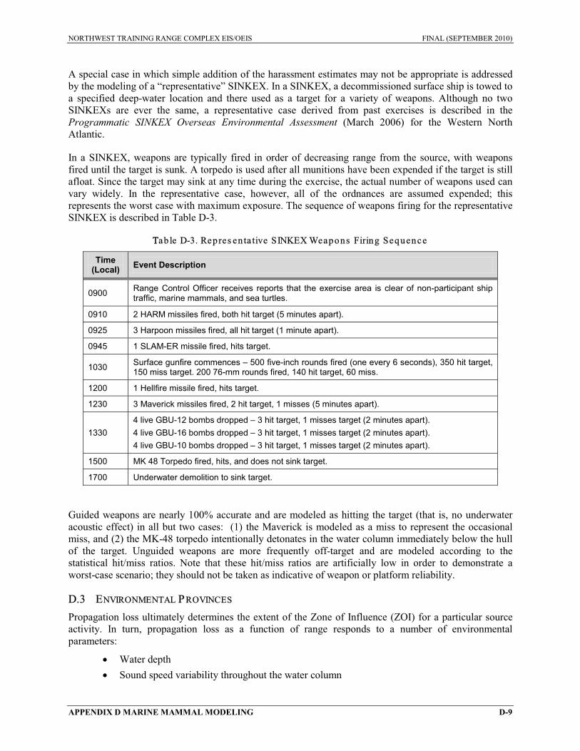
In a SINKEX, weapons are typically fired in order of decreasing range from the source, with weapons fired until the target is sunk. A torpedo is used after all munitions have been expended if the target is still afloat. Since the target may sink at any time during the exercise, the actual number of weapons used can vary widely. In the representative case, however, all of the ordnances are assumed expended; this represents the worst case with maximum exposure. The sequence of weapons firing for the representative SINKEX is described in Table D-3.
TTable D-3. Repres en ta tive SINKEX Weapons Firing Sequence
Time (Local) Event Description
0900 Range Control Officer receives reports that the exercise area is clear of non-participant ship traffic, marine mammals, and sea turtles.
0910 2 HARM missiles fired, both hit target (5 minutes apart).
0925 3 Harpoon missiles fired, all hit target (1 minute apart).
0945 1 SLAM-ER missile fired, hits target.
1030 Surface gunfire commences – 500 five-inch rounds fired (one every 6 seconds), 350 hit target, 150 miss target. 200 76-mm rounds fired, 140 hit target, 60 miss.
1200 1 Hellfire missile fired, hits target.
1230 3 Maverick missiles fired, 2 hit target, 1 misses (5 minutes apart).
13304 live GBU-12 bombs dropped – 3 hit target, 1 misses target (2 minutes apart).4 live GBU-16 bombs dropped – 3 hit target, 1 misses target (2 minutes apart).4 live GBU-10 bombs dropped – 3 hit target, 1 misses target (2 minutes apart).
1500 MK 48 Torpedo fired, hits, and does not sink target.
1700 Underwater demolition to sink target.
Guided weapons are nearly 100% accurate and are modeled as hitting the target (that is, no underwater acoustic effect) in all but two cases: (1) the Maverick is modeled as a miss to represent the occasional miss, and (2) the MK-48 torpedo intentionally detonates in the water column immediately below the hull of the target. Unguided weapons are more frequently off-target and are modeled according to the statistical hit/miss ratios. Note that these hit/miss ratios are artificially low in order to demonstrate a worst-case scenario; they should not be taken as indicative of weapon or platform reliability.
D.3 ENVIRONMENTAL P ROVINCES
Propagation loss ultimately determines the extent of the Zone of Influence (ZOI) for a particular source activity. In turn, propagation loss as a function of range responds to a number of environmental parameters:
• Water depth• Sound speed variability throughout the water column

NORTHWEST TRAINING RANGE COMPLEX EIS/OEIS FINAL (SEPTEMBER 2010)
APPENDIX D MARINE MAMMAL MODELING D-10
• Bottom geo-acoustic properties, and• Surface roughness, as determined by wind speed
Due to the importance that propagation loss plays in ASW, the Navy has, over the last four to five decades, invested heavily in measuring and modeling these environmental parameters. The result of this effort is the following collection of global databases of these environmental parameters, which are accepted as standards for Navy modeling efforts.
• Water depth—Digital Bathymetry Data Base Variable Resolution (DBDBV)• Sound speed—Generalized Digital Environmental Model (GDEM)• Bottom loss—Low-Frequency Bottom Loss (LFBL), Sediment Thickness Database, and
High-Frequency Bottom Loss (HFBL), and• Wind speed—U.S. Navy Marine Climatic Atlas of the World
This section provides a discussion of the relative impact of these various environmental parameters. These examples then are used as guidance for determining environmental provinces (that is, regions in which the environmental parameters are relatively homogeneous and can be represented by a single set of environmental parameters) within the NWTRC.
D.3.1 Impact of Environmental ParametersWithin a typical operating area, the environmental parameter that tends to vary the most is bathymetry. It is not unusual for water depths to vary by an order of magnitude or more, resulting in significant impacts on the ZOI calculations. Bottom loss can also vary considerably over typical operating areas, but its impact on ZOI calculations tends to be limited to waters on the continental shelf and the upper portion of the slope. Generally, the primary propagation paths in deep water, from the source to most of the ZOI volume, do not involve any interaction with bottom. In shallow water, particularly if the sound velocity profile directs all propagation paths to interact with the bottom, bottom loss variability can play a larger role.
The spatial variability of the sound speed field is generally small over operating areas of typical size. The presence of a strong oceanographic front is a noteworthy exception to this rule. To a lesser extent, variability in the depth and strength of a surface duct can be of some importance. In the mid-latitudes, seasonal variation often provides the most significant variation in the sound speed field. For this reason, both summer and winter profiles are modeled for each selected environment.
D.3.2 Environmental Provincing MethodologyThe underwater acoustic environment can be quite variable over ranges in excess of 10 kilometers (km).For ASW applications, ranges of interest are often sufficiently large as to warrant the modeling of the spatial variability of the environment. In the propagation loss calculations, each of the environmental parameters is allowed to vary (either continuously or discretely) along the path from acoustic source to receiver. In such applications, each propagation loss calculation is conditioned upon the particular locations of the source and receiver.
On the other hand, the range of interest for marine animal harassment by most Naval activities is more limited. This reduces the importance of the exact location of source and marine animal and makes the modeling required more manageable in scope.
In lieu of trying to model every environmental profile that can be encountered in an operating area, this effort utilizes a limited set of representative environments. Each environment is characterized by a fixed water depth, sound velocity profile, and bottom loss type. The operating area is then partitioned into homogeneous regions (or provinces), and the most appropriately representative environment is assigned to each. This process is aided by some initial provincing of the individual environmental parameters. The

NORTHWEST TRAINING RANGE COMPLEX EIS/OEIS FINAL (SEPTEMBER 2010)
APPENDIX D MARINE MAMMAL MODELING D-11
Navy-standard high-frequency bottom loss database in its native form is globally partitioned into nine classes. Low-frequency bottom loss is likewise provinced in its native form, although it is not considered in the process of selecting environmental provinces. Only the broadband sources produce acoustic energy at the frequencies of interest for low-frequency bottom loss (typically less than 1 kHz); even for those sources the low-frequency acoustic energy is secondary to the energy above 1 kHz. The Navy-standard sound velocity profiles database is also available as a provinced subset. Only the Navy-standard bathymetry database varies continuously over the world’s oceans. However, even this environmental parameter is easily provinced by selecting a finite set of water depth intervals. For this analysis “octave-spaced” intervals (10, 20, 50, 100, 200, 500, 1,000, 2,000, and 5,000 meters) provide an adequate sampling of water depth dependence.
ZOI volumes are then computed using propagation loss estimates derived for the representative environments. Finally, a weighted average of the ZOI volumes is taken over all representative environments; the weighting factor is proportional to the geographic area spanned by the environmental province.
The selection of representative environments is subjective. However, the uncertainty introduced by this subjectivity can be mitigated by selecting more environments and by selecting the environments that occur most frequently over the operating area of interest.
As discussed in the previous subsection, ZOI estimates are most sensitive to water depth. Unless otherwise warranted, at least one representative environment is selected in each bathymetry province. Within a bathymetry province, additional representative environments are selected as needed to meet the following requirements.
• In shallow water (less than 1,000 meters), bottom interactions occur at shorter ranges and more frequently; thus significant variations in bottom loss need to be represented.
• Surface ducts provide an efficient propagation channel that can greatly influence ZOI estimates. Variations in the mixed layer depth need to be accounted for if the water is deep enough to support the full extent of the surface duct.
Depending upon the size and complexity of the operating area, the number of environmental provinces tends to range from 5 to 20.
D.3.3 Description of Environmental ProvincesThe NWTRC encompasses a large area off the U.S. West Coast. For this analysis, the general operating area is bounded to the north and south by 48o 30’ N and 40o N and to the west by meridian of 130o W and to the east by land. Within this large region a sub-area used for SINKEX operations is defined by the following additional restrictions:
• More than 50 nautical miles (nm) from land, and
• Water depth greater than 1,000 fathoms (1,852 meters).
Some of the active sonars are limited to Warning Area 237 (W-237), an irregularly-shaped region with the following vertices:
48° 21’ 03” N 130° 00’ 00” W
48° 20’ 00” N 128° 00’ 00” W
48° 08’ 59” N 125° 55’ 00” W
46° 32’ 00” N 126° 42’ 00” W
45° 50’ 00” N 128° 10’ 00” W

NORTHWEST TRAINING RANGE COMPLEX EIS/OEIS FINAL (SEPTEMBER 2010)
APPENDIX D MARINE MAMMAL MODELING D-12
The surface ship sonars are deployed throughout the general operating area. The air-deployed sonars, including the AN/SSQ-110, are limited to W-237. The explosive sources and demolition charges are limited to the SINKEX subarea.
This subsection describes the representative environmental provinces selected for the NWTRC. For all of these provinces, the average winter wind speed is 14 knots, whereas the average summer wind speed is 8 knots.
The general operating area of the NWTRC contains a total of 47 distinct environmental provinces. These represent various combinations of nine bathymetry provinces, four Sound Velocity Profile (SVP) provinces, and six HFBL classes. Among these 47 provinces, some share important characteristics while others occur infrequently, so the provinces were reduced to a generalized class of 16 fundamental provinces.
The bathymetry provinces represent depths ranging from very shallow to typical deep-water depths. However, nearly 90% of the NWTRC is characterized as deep-water (depths of 1,000 meters or more). The distribution of the bathymetry provinces over the NWTRC is provided in Table D-4.
Four SVP provinces describe the sound speed field in the NWTRC; however, only two (provinces 30 and 35) make any significant contribution to the analysis. The variability among the four provinces is relatively small as demonstrated by the summer profiles presented in Figure D-1. The dominant difference among the profiles is the relative strength of a suppressed secondary sound channel. Thisfeature is most clearly in the two dominant provinces.
TTable D-4. Dis tribu tion o f Bath ymetry P rovinces in NWTRC
Province Depth (m) Frequency of Occurrence
10 0.32 %20 0.68 %50 2.24 %
100 3.71 %200 3.12 %500 3.00 %
1,000 4.55 %2,000 55.48 %5,000 26.90 %

NORTHWEST TRAINING RANGE COMPLEX EIS/OEIS FINAL (SEPTEMBER 2010)
APPENDIX D MARINE MAMMAL MODELING D-13
FFigure D-1. Summer SVPs in NWTRC
The variation in the winter SVPs among the provinces is a bit more pronounced (Figure D-2). All four provinces display a surface duct but the two dominant provinces have a much deeper mixed layer (as much as 350 meters). This feature provides an efficient propagation channel when source and receiver are both located above the mixed layer.
Figure D-2. Winter SVPs in NWTRC
The distribution of the SVP provinces across the NWTRC is provided in Table D-5.
Table D-5. Dis tribu tion o f SVP Provinces in NWTRC
SVP Province Frequency of Occurrence
30 87.39 %
34 0.78 %
35 11.53 %
38 0.30 %
0
200
400
600
800
1000
1470 1480 1490 1500 1510
Sound Speed (m/s)
Dept
h (m
) 30343538
0100200300400500600700800900
1000
1470 1480 1490 1500
Sound Speed (m/s)
Dept
h (m
) 30343538

NORTHWEST TRAINING RANGE COMPLEX EIS/OEIS FINAL (SEPTEMBER 2010)
APPENDIX D MARINE MAMMAL MODELING D-14
The six HFBL classes represented in the NWTRC range from low-loss bottoms (class 2 and 3) to high-loss bottoms (classes 7 and 8). The distribution of HFBL classes summarized in Table D-6 indicates that both low- and high-loss classes are approximately equally distributed.
TTable D-6. Dis tribu tion of High-Frequency Bottom Los s Cla s s e s in NWTRC
HFBL Class Frequency of Occurrence
2 23.60 %
3 6.15 %
4 21.79 %
6 18.20 %
7 2.26 %
8 28.00 %
The logic for consolidating the environmental provinces focuses on water depth, using the sound speed profile (in deep water) and the HFBL class (in shallow water) as secondary differentiating factors. The first consideration was to ensure that all nine bathymetry provinces are represented. Then within each bathymetry province further partitioning of provinces proceeded as follows:
• The four shallowest bathymetry provinces are each represented by one environmental province. In each case, the bathymetry province is dominated by a single, low-loss bottom, so that the secondary differentiating environmental parameter is of no consequence.
• The 200- and 500-meter bathymetry provinces each consist of two environmental provinces in order to reflect both low- and high-loss bottoms that are prevalent at these depths. The 1,000-meter bathymetry province includes only high-loss bottoms and therefore does not need to be partitioned
• The 2,000-meter bathymetry province contains negligible variability in sound speed profiles. However, the 2,000-meter bathymetry province is significantly large as to warrant some partitioning based upon bottom loss. This bathymetry province is subdivided into three environmental provinces using HFBL classes 4, 6 and 8.
• The 5,000-meter bathymetry province is also a prevalent water depth in the NWTRC. For this analysis, it is partitioned into four environment provinces to capture both SVP province (30 and 35), and bottoms that are low-loss (HFBL classes 2 and 3) and high-loss (HFBL class 7).
The resulting 16 environmental provinces used in the NWTRC acoustic modeling are described in Table D-7.
The percentages given in the preceding table indicate the frequency of occurrence of each environmental province across the general operating area in the NWTRC. Geographically, the distribution of these 16 environmental provinces is exhibited in Figure D-3.

NORTHWEST TRAINING RANGE COMPLEX EIS/OEIS FINAL (SEPTEMBER 2010)
APPENDIX D MARINE MAMMAL MODELING D-15
TTable D-7. Dis tribu tion o f Environmenta l Provinces in Genera l OP AREA of NWTRC
Environmental Province
Water Depth
SVP Province
HFBL Class
LFBL Province
Sediment Thickness
Frequency of Occurrence
1 10 m 30 2 0 0.2 secs 0.324%
2 20 m 30 2 0 0.2 secs 0.688%
3 50 m 30 2 0 0.27 secs 2.268%
4 100 m 30 2 – 10 0.41 secs 3.751%
5 200 m 30 2 – 10* 0.33 secs 2.577%
6 200 m 30 8 – 10* 0.62 secs 0.582%
7 500 m 30 8 14 0.31 secs 2.484%
8 500 m 30 2 – 10 0.23 secs 0.550%
9 1,000 m 30 8 14 0.21 secs 4.605%
10 2,000 m 30 4 18 0.82 secs 29.627%
11 2,000 m 30 8 18 0.41 secs 15.460%
12 2,000 m 30 6 19 0.2 secs 11.026%
13 5,000 m 30 2 14 0.74 secs 8.396%
14 5,000 m 35 3 18 0.36 secs 3.960%
15 5,000 m 30 7 14 0.88 secs 7.815%
16 5,000 m 35 7 18 0.29 secs 5.886% * Negative province numbers indicate shallow water provinces

NORTHWEST TRAINING RANGE COMPLEX EIS/OEIS FINAL (SEPTEMBER 2010)
APPENDIX D MARINE MAMMAL MODELING D-16
Note: the northwestern coast of the United States is in blue, and higher province index numbers correspond to redder colors. The white polygon represents W-237.
FFigure D-3. NWTRC Environmenta l Provinces over OPAREA
Longitude
Latit
ude
-130 -128.89 -127.78 -126.67 -125.57 -124.46 -123.35 -122.24
48.48
47.27
46.06
44.85
43.63
42.42
41.21

NORTHWEST TRAINING RANGE COMPLEX EIS/OEIS FINAL (SEPTEMBER 2010)
APPENDIX D MARINE MAMMAL MODELING D-17
The distribution of the environments within the SINKEX area is, by definition, limited to the two deepest bathymetry provinces as indicated in Table D-8.
TTable D-8. Dis tribu tion o f Environmenta l Provinces with in SINKEX Area
Environmental Province Frequency of Occurrence
10 38.48 %
11 13.92 %
12 14.21 %
13 9.67 %
14 5.13 %
15 9.19 %
16 9.40 %
The air-deployed sonars are also restricted in their use. They are limited to W-237 for which the distribution of provinces is provided in Table D-9.
Table D-9. Dis tribu tion o f Environmenta l Provinces with in W-237
Environmental Province Frequency of Occurrence
5 1.112 %
6 0/015 %
7 0.846 %
8 0.395 %
9 3.111 %
10 71.883 %
11 7.976 %
12 14.662 %
D.4 IMPACT VOLUMES AND IMPACT RANGES
Many naval actions include the potential to injure or harass marine animals in the neighboring waters through noise emissions. The number of animals exposed to potential harassment in any such action is dictated by the propagation field and the characteristics of the noise source.
The impact volume associated with a particular activity is defined as the volume of water in which some acoustic metric exceeds a specified threshold. The product of this impact volume with a volumetric animal density yields the expected value of the number of animals exposed to that acoustic metric at a level that exceeds the threshold. The acoustic metric can either be an energy term (EFD, either in a limited frequency band or across the full band) or a pressure term (such as peak pressure or positive impulse). The thresholds associated with each of these metrics define the levels at which half of the animals exposed will experience some degree of harassment (ranging from behavioral change to mortality).
Impact volume is particularly relevant when trying to estimate the effect of repeated source emissions separated in either time or space. Impact range, which is defined as the maximum range at which a

NORTHWEST TRAINING RANGE COMPLEX EIS/OEIS FINAL (SEPTEMBER 2010)
APPENDIX D MARINE MAMMAL MODELING D-18
particular threshold is exceeded for a single source emission, defines the range to which marine mammal activity is monitored in order to meet mitigation requirements.
With the exception of explosive sources, the sole relevant measure of potential harm to the marine wildlife due to sonar is the accumulated (summed over all source emissions) EFD received by the animal over the duration of the activity. Harassment measures for explosive sources include EFD and pressure-related metrics (peak pressure and positive impulse).
Regardless of the type of source, estimating the number of animals that may be injured or otherwise harassed in a particular environment entails the following steps.
Each source emission is modeled according to the particular operating mode of the sonar. The “effective” energy source level is computed by integrating over the bandwidth of the source, scaling by the pulse length, and adjusting for gains due to source directivity. The location of the source at the time of each emission must also be specified.
For the relevant environmental acoustic parameters, transmission loss (TL) estimates are computed, sampling the water column over the appropriate depth and range intervals. TL data are sampled at the typical depth(s) of the source and at the nominal center frequency of the source. If the source is relatively broadband, an average over several frequency samples is required.
The accumulated energy within the waters that the source is “operating” is sampled over a volumetric grid. At each grid point, the received energy from each source emission is modeled as the effective energy source level reduced by the appropriate propagation loss from the location of the source at the time of the emission to that grid point and summed. For the peak pressure or positive impulse, the appropriate metric is similarly modeled for each emission. The maximum value of that metric, over all emissions, is stored at each grid point.
The impact volume for a given threshold is estimated by summing the incremental volumes represented by each grid point for which the appropriate metric exceeds that threshold.
Finally, the number of exposures is estimated as the “product” (scalar or vector, depending on whether an animal density depth profile is available) of the impact volume and the animal densities.
This section describes in detail the process of computing impact volumes (that is, the first four steps described above). This discussion is presented in two parts: active sonars and explosive sources. The relevant assumptions associated with this approach and the limitations that are implied are also presented. The final step, computing the number of exposures, is discussed in subsection D.6.
D.4.1 Computing Impact Volumes for Active SonarsThis section provides a detailed description of the approach taken to compute impact volumes for active sonars. Included in this discussion are:
• Identification of the underwater propagation model used to compute transmission loss data, a listing of the source-related inputs to that model, and a description of the output parameters that are passed to the energy accumulation algorithm.
• Definitions of the parameters describing each sonar type.
• Description of the algorithms and sampling rates associated with the energy accumulation algorithm.

NORTHWEST TRAINING RANGE COMPLEX EIS/OEIS FINAL (SEPTEMBER 2010)
APPENDIX D MARINE MAMMAL MODELING D-19
D.4.1.1 Transmission Loss Calculations
TL data are pre-computed for each of two seasons in each of the environmental provinces described in the previous subsection using the GRAB propagation loss model (Keenan, 2000). The TL output consists of a parametric description of each significant eigenray (or propagation path) from source to animal. The description of each eigenray includes the departure angle from the source (used to model the source vertical directivity later in this process), the propagation time from the source to the animal (used to make corrections to absorption loss for minor differences in frequency and to incorporate a surface-image interference correction at low frequencies), and the TL suffered along the eigenray path.
The eigenray data for a single GRAB model run are sampled at uniform increments in range out to a maximum range for a specific “animal” (or “target” in GRAB terminology) depth. Multiple GRAB runs are made to sample the animal depth dependence. The depth and range sampling parameters are summarized in Table D-10. Note that some of the low-power sources do not require TL data to large maximum ranges.
TTable D-10. TL Depth and Range Sampling Parameters b y Sona r Typ e
Sonar Range Step Maximum Range Depth Sampling
MK-48 10 m 10 km 0 – 1 km in 5-m steps1 km – Bottom in 10-m steps
AN/SQS-53C 10 m 200 km 0 – 1 km in 5-m steps1 km – Bottom in 10-m steps
AN/ASQ-62 5 m 5 km 0 – 1 km in 5-m steps1 km – Bottom in 10-m steps
AN/SQS-56 10 m 50 km 0 – 1 km in 5-m steps1 km – Bottom in 10-m steps
In a few cases, most notably the AN/SQS-53C for thresholds below approximately 180 dB, TL data may be required by the energy summation algorithm at ranges greater than covered by the pre-computed GRAB data. In these cases, TL is extrapolated to the required range using a simple cylindrical spreading loss law in addition to the appropriate absorption loss. This extrapolation leads to a conservative (or under) estimate of TL at the greater ranges.
Although GRAB provides the option of including the effect of source directivity in its eigenray output, this capability is not exercised. By preserving data at the eigenray level, this allows source directivity to be applied later in the process and results in fewer TL calculations.
The other important feature that storing eigenray data supports is the ability to model the effects of surface-image interference that persist over range. However, this is primarily important at frequencies lower than those associated with the sonars considered in this subsection. A detailed description of the modeling of surface-image interference is presented in the subsection on explosive sources.
D.4.1.2 Energy Summation
The summation of EFD over multiple pings in a range-independent environment is a trivial exercise for the most part. A volumetric grid that covers the waters in and around the area of sonar operation is initialized. The source then begins its set of pings. For the first ping, the TL from the source to each grid point is determined (summing the appropriate eigenrays after they have been modified by the vertical beam pattern), the “effective” energy source level is reduced by that TL, and the result is added to the accumulated EFD at that grid point. After each grid point has been updated, the accumulated energy at

NORTHWEST TRAINING RANGE COMPLEX EIS/OEIS FINAL (SEPTEMBER 2010)
APPENDIX D MARINE MAMMAL MODELING D-20
grid points in each depth layer is compared to the specified threshold. If the accumulated energy exceeds that threshold, then the incremental volume represented by that grid point is added to the impact volume for that depth layer. Once all grid points have been processed, the resulting sum of the incremental volumes represents the impact volume for one ping.
The source is then moved along one of the axes in the horizontal plane by the specified ping separation range and the second ping is processed in a similar fashion. Again, once all grid points have been processed, the resulting sum of the incremental volumes represents the impact volume for two pings. This procedure continues until the maximum number of pings specified has been reached.
Defining the volumetric grid over which energy is accumulated is the trickiest aspect of this procedure. The volume must be large enough to contain all volumetric cells for which the accumulated energy is likely to exceed the threshold but not so large as to make the energy accumulation computationally unmanageable.
Determining the size of the volumetric grid begins with an iterative process to determine the lateral extent to be considered. Unless otherwise noted, throughout this process the source is treated as omnidirectional and the only animal depth that is considered is the TL target depth that is closest to the source depth (placing source and receiver at the same depth is generally an optimal TL geometry).
The first step is to determine the impact range (Rmax) for a single ping. The impact range in this case is the maximum range at which the effective energy source level reduced by the TL is greater than the threshold. Next, the source is moved along a straight-line track and EFD is accumulated at a point that has a closest point of approach (CPA) range of RMAX at the mid-point of the source track. That total EFD summed over all pings is then compared to the prescribed threshold. If it is greater than the threshold (which, for the first Rmax, it must be) then Rmax is increased by 10 percent, the accumulation process is repeated, and the total energy is again compared to the threshold. This continues until Rmax grows large enough to ensure that the accumulated EFD at that lateral range is less than the threshold. The lateral range dimension of the volumetric grid is then set at twice Rmax, with the grid centered along the source track. In the direction of advance for the source, the volumetric grid extends on the interval from [–Rmax, 3 Rmax] with the first source position located at zero in this dimension. Note that the source motion in this direction is limited to the interval [0, 2 Rmax]. Once the source reaches 2 Rmax in this direction, the incremental volume contributions have approximately reached their asymptotic limit and further pings add essentially the same amount. This geometry is demonstrated in Figure D-4.
If the source is directive in the horizontal plane, then the lateral dimension of the grid may be reduced and the position of the source track adjusted accordingly. For example, if the main lobe of the horizontal source beam is limited to the starboard side of the source platform, then the port side of the track is reduced substantially as demonstrated in Figure D-5.
Once the extent of the grid is established, the grid sampling can be defined. In both dimensions of the horizontal plane the sampling rate is approximately Rmax/100. The round-off error associated with this sampling rate is roughly equivalent to the error in a numerical integration to determine the area of a circle with a radius of Rmax with a partitioning rate of Rmax/100 (approximately 1 percent). The depth-sampling rate of the grid is comparable to the sampling rates in the horizontal plane but discretized to match an actual TL sampling depth. The depth-sampling rate is also limited to no more than 10 meters to ensure that significant TL variability over depth is captured.

NORTHWEST TRAINING RANGE COMPLEX EIS/OEIS FINAL (SEPTEMBER 2010)
APPENDIX D MARINE MAMMAL MODELING D-21
FFigure D-4. Horizontal P lane of Volumetric Grid for Omni Direc tiona l Source
Figure D-5. Horizontal P lane of Volumetric Grid for S tarboard Beam Source
Rmax
–Rmax
3 Rmax–Rmax
Direction of Advance
Lateral Direction
Limit of Energy Grid in Horizontal Plane
0.1 Rmax–Rmax 3 Rmax
–Rmax
Direction of Advance
Lateral Direction
Limit of Energy Grid in Horizontal Plane

NORTHWEST TRAINING RANGE COMPLEX EIS/OEIS FINAL (SEPTEMBER 2010)
APPENDIX D MARINE MAMMAL MODELING D-22
D.4.1.3 Impact Volume per Hour of Sonar Operation
The impact volume for a sonar moving relative to the animal population increases with each additional ping. The rate at which the impact volume increases varies with a number of parameters but eventually approaches some asymptotic limit. Beyond that point the increase in impact volume becomes essentially linear as depicted in Figure D-6.
FFigure D-6. 53C Impact Volume by Ping
The slope of the asymptotic limit of the impact volume at a given depth is the impact volume added per ping. This number multiplied by the number of pings in an hour gives the hourly impact volume for the given depth increment. Completing this calculation for all depths in a province, for a given source, gives the hourly impact volume vector, nv , which contains the hourly impact volumes by depth for province n. Figure D-7 provides an example of an hourly impact volume vector for a particular environment.
Figure D-7. Example of an Impact Volume Vector
0 0.5 1 1.5 2 2.5 3
x 1010
-2000
-1800
-1600
-1400
-1200
-1000
-800
-600
-400
-200
0
Ensonified Volume (cubic meters)
Dep
th (m
eter
s)
Ensonified Volume After 100 Pings by depth

NORTHWEST TRAINING RANGE COMPLEX EIS/OEIS FINAL (SEPTEMBER 2010)
APPENDIX D MARINE MAMMAL MODELING D-23
D.4.2 Computing Impact Volumes for Explosive SourcesThis section provides the details of the modeling of the explosive sources. This energy summation algorithm is similar to that used for sonars, only differing in details such as the sampling rates and source parameters. These differences are summarized in the following subsections. A more significant difference is that the explosive sources require the modeling of additional pressure metrics: (1) peak pressure, and (2) “modified” positive impulse. The modeling of each of these metrics is described in detail in the subsections of D.4.2.3.
D.4.2.1 Transmission Loss Calculations
Modeling impact volumes for explosive sources span requires the same type of TL data as needed for active sonars. However, unlike active sonars, explosive ordnances and the EER source are broadband, contributing significant energy from tens of hertz to tens of kilohertz. To accommodate the broadband nature of these sources, TL data are sampled at seven frequencies from 10 Hz to 40 kHz, spaced every two octaves.
An important propagation consideration at low frequencies is the effect of surface-image interference. As either source or target approach the surface, pairs of paths that differ by a single surface reflection set up an interference pattern that ultimately causes the two paths to cancel each other when the source or target is at the surface. A fully coherent summation of the eigenrays produces such a result but also introduces extreme fluctuations that would have to be highly sampled in range and depth, and then smoothed to give meaningful results. An alternative approach is to implement what is sometimes called a semi-coherent summation. A semi-coherent sum attempts to capture significant effects of surface-image interference (namely the reduction of the field due to destructive interference of reflected paths as the source or target approach the surface) without having to deal with the more rapid fluctuations associated with a fully coherent sum. The semi-coherent sum is formed by a random phase addition of paths that have already been multiplied by the expression:
sin2 [ 4 π f zs za / (c2 t) ]
where f is the frequency, zs is the source depth, za is the animal depth, c is the sound speed and t is the travel time from source to animal along the propagation path. For small arguments of the sine function this expression varies directly as the frequency and the two depths. It is this relationship that causes the propagation field to go to zero as the depths approach the surface or the frequency approaches zero.
This surface-image interference must be applied across the entire bandwidth of the explosive source. The TL field is sampled at several representative frequencies. However, the image-interference correction given above varies substantially over that frequency spacing. To avoid possible under sampling, the image-interference correction is averaged over each frequency interval.
D.4.2.2 Source Parameters
Unlike active sonars, explosive sources are defined by only two parameters: (1) net explosive weight, and (2) source detonation depth. Values for these source parameters are defined earlier in subsection D.2.2.
The effective energy source level, which is treated as a de facto input for the other sonars, is instead modeled directly for EER and munitions. For both, the energy source level is comparable to the model used for other explosives (Arons [1954], Weston [1960], McGrath [1971], Urick [1983], Christian and Gaspin [1974]). The energy source level over a one-third octave band with a center frequency of f for a source with a net explosive weight of w pounds is given by:
ESL = 10 log10 (0.26 f ) + 10 log10 ( 2 pmax2 / [1/θ 2 + 4 π f 2] ) + 197 dB

NORTHWEST TRAINING RANGE COMPLEX EIS/OEIS FINAL (SEPTEMBER 2010)
APPENDIX D MARINE MAMMAL MODELING D-24
where the peak pressure for the shock wave at 1 meter is defined as
pmax = 21600 (w1/3 / 3.28 )1.13 psi (E-1)
and the time constant is defined as:
θ = [(0.058) (w1/3) (3.28 / w1/3) 0.22 ] / 1,000 msec (E-2)
In contrast to munitions that are modeled as omnidirectional sources, the EER source is a continuous line array that produces a directed source. The EER array consists of two explosive strips that are fired individually from the center of the array. Each strip generates a beam pattern with the steer direction of the main lobe determined by the burn rate. The resulting response of the entire array is a bifurcated beam for frequencies above 200 Hz, while at lower frequencies the two beams tend to merge into one.
Since very short ranges are under consideration, the loss of directivity of the array needs to be accounted for in the near field of the array. This is accomplished by modeling the sound pressure level across the field as the coherent sum of contributions of infinitesimal sources along the array that are delayed according to the burn rate. For example, for frequency f the complex pressure contribution at a depth z and horizontal range x from an infinitesimal source located at a distance z’ above the center of the array is
p(r,z) = e iφ
where
φ = kr’ + αz’, and
α = 2 πf / cb
with k the acoustic wave number, cb the burn rate of the explosive ribbon, and r’ the slant range from the infinitesimal source to the field point (x,z).
Beam patterns as function of vertical angle are then sampled at various ranges out to a maximum range that is approximately L2 / λ where L is the array length and λ is the wavelength. This maximum range is a rule-of-thumb estimate for the end of the near field (Bartberger, 1965). Finally, commensurate with the resolution of the TL samples, these beam patterns are averaged over octave bands.
A couple of sample beam patterns are provided in Figure D-8 and Figure D-9. In both cases, the beam response is sampled at various ranges from the source array to demonstrate the variability across the near field. The 80-Hz family of beam patterns presented in Figure D-8 shows the rise of a single main lobe as range increases.

NORTHWEST TRAINING RANGE COMPLEX EIS/OEIS FINAL (SEPTEMBER 2010)
APPENDIX D MARINE MAMMAL MODELING D-25
FFigure D-8. 80-Hz Beam Patte rns acros s Near Field of EER Source
On the other hand, the 1,250-Hz family of beam patterns depicted in Figure D-9 demonstrates the typical high-frequency bifurcated beam.
Figure D-9. 1250-Hz Beam Patte rns acros s Near Field of EER SourceD.4.2.3 Impact Volumes for Various Metrics
The impact of explosive sources on marine wildlife is measured by three different metrics, each with its own thresholds. The energy metric, peak one-third octave, is treated in similar fashion as the energy metric used for the active sonars, including the summation of energy if there are multiple source emissions. The other two, peak pressure and positive impulse, are not accumulated but rather the maximum levels are taken.
-12-10
-8-6-4-20246
-90 -60 -30 0 30 60 90
Bea
m R
espo
nse
(dB
re O
mni
)
Vertical Angle (deg)
80-Hz Beam PatternSampled Every Meter to a Range of 25 Meters
-25-20-15-10-505
10
-90 -60 -30 0 30 60 90
Bea
m R
espo
nse
(dB
re
Om
ni)
Vertical Angle (deg)
1250-Hz Beam PatternSampled Every Four Meters to a Range of 400 Meters

NORTHWEST TRAINING RANGE COMPLEX EIS/OEIS FINAL (SEPTEMBER 2010)
APPENDIX D MARINE MAMMAL MODELING D-26
PPeak One-Third Octave Energ y MetricThe computation of impact volumes for the energy metric closely follows the approach taken to model the energy metric for the active sonars. The only significant difference is that EFD is sampled at several frequencies in one-third-octave bands and only the peak one-third-octave level is accumulated over time.
Peak P res s ure MetricThe peak pressure metric is a simple, straightforward calculation at each range/animal depth combination. First, the transmission ratio, modified by the source level in a one-octave band and the vertical beam pattern, is averaged across frequency on an eigenray-by-eigenray basis. This averaged transmission ratio (normalized by the total broadband source level) is then compared across all eigenrays with the maximum designated as the peak arrival. Peak pressure at that range/animal depth combination is then simply the product of:
• The square root of the averaged transmission ratio of the peak arrival,
• The peak pressure at a range of 1 meter (given by equation E-1), and
• The similitude correction (given by r –0.13, where r is the slant range along the eigenray estimated as tc with t the travel time along the dominant eigenray and c the nominal speed of sound).
If the peak pressure for a given grid point is greater than the specified threshold, then the incremental volume for the grid point is added to the impact volume for that depth layer.
“Modified” Pos itive Impuls e MetricThe modeling of positive impulse follows the work of Goertner (Goertner, 1982). The Goertner model defines a “partial” impulse as
Tmin
∫ p(t) dt
0
where p(t) is the pressure wave from the explosive as a function of time t, defined so that p(t) = 0 for t < 0. This pressure wave is modeled as
p(t) = pmax e –t/θ
where pmax is the peak pressure at 1 meter (see, equation B-1), and θ is the time constant defined as
θ = 0.058 w1/3 (r/w1/3) 0.22 seconds
with w the net explosive weight (pounds), and r the slant range between source and animal.
The upper limit of the “partial” impulse integral is
Tmin = min {Tcut, Tosc}
where Tcut is the time to cutoff and Tosc is a function of the animal lung oscillation period. When the upper limit is Tcut, the integral is the definition of positive impulse. When the upper limit is defined by Tosc, the integral is smaller than the positive impulse and thus is just a “partial” impulse. Switching the integral
NORTHWEST TRAINING RANGE COMPLEX EIS/OEIS FINAL (SEPTEMBER 2010)
APPENDIX D MARINE MAMMAL MODELING D-27
limit from Tcut to Tosc accounts for the diminished impact of the positive impulse upon the animals lungs that compress with increasing depth and leads to what is sometimes call a “modified” positive impulse metric.
The time to cutoff is modeled as the difference in travel time between the direct path and the surface-reflected path in an isospeed environment. At a range of r, the time to cutoff for a source depth zs and an animal depth za is
Tcut = 1/c { [r2 + (za + zs)2]1/2 – [r2 + (za – zs)2]1/2 }
where c is the speed of sound.
The animal lung oscillation period is a function of animal mass M and depth za and is modeled as
Tosc = 1.17 M1/3 (1 + za/33) –5/6
where M is the animal mass (in kg) and za is the animal depth (in feet).
The modified positive impulse threshold is unique among the various injury and harassment metrics in that it is a function of depth and the animal weight. So instead of the user specifying the threshold, it is computed as K (M/42)1/3 (1 + za/33)1/2. The coefficient K depends upon the level of exposure. For the onset of slight lung injury, K is 19.7; for the onset of extensive lung hemorrhaging (1% mortality), K is 47.
Although the thresholds are a function of depth and animal weight, sometimes they are summarized as their value at the sea surface for a typical dolphin calf (with an average mass of 12.2 kg). For the onset of slight lung injury, the threshold at the surface is approximately 13 psi-msec; for the onset of extensive lung hemorrhaging (1% mortality), the threshold at the surface is approximately 31 psi-msec.
As with peak pressure, the “modified” positive impulse at each grid point is compared to the derived threshold. If the impulse is greater than that threshold, then the incremental volume for the grid point is added to the impact volume for that depth layer.
D.4.2.4 Impact Volume per Explosive Detonation
The detonations of explosive sources are generally widely spaced in time and/or space. This implies that the impact volume for multiple firings can be easily derived by scaling the impact volume for a single detonation. Thus the typical impact volume vector for an explosive source is presented on a per-detonation basis.
D.4.3 Impact Volume by RegionThe NWTRC is described by 16 environmental provinces. The hourly impact volume vector for operations involving any particular source is a linear combination of the 16 impact volume vectors with the weighting determined by the distribution of those 16 environmental provinces within the range. Unique hourly impact volume vectors for winter and summer are calculated for each type of source and each metric/threshold combination.
DD.5 RISK FUNCTION: THEORETICAL AND P RACTICAL IMPLEMENTATION
This section discusses the recent addition of a risk function “threshold” to acoustic effects analysis procedure. This approach includes two parts, a metric, and a function to map exposure level under the metric to probability of harassment. What these two parts mean, how they affect exposure calculations, and how they are implemented are the objects of discussion.

NORTHWEST TRAINING RANGE COMPLEX EIS/OEIS FINAL (SEPTEMBER 2010)
APPENDIX D MARINE MAMMAL MODELING D-28
D.5.1 Thresholds and MetricsThe term “thresholds” is broadly used to refer to both thresholds and metrics. The difference, and the distinct roles of each in effects analyses, will be the foundation for understanding the risk function approach, putting it in perspective, and showing that, conceptually, it is similar to past approaches.
Sound is a pressure wave, so at a certain point in space, sound is simply rapidly changing pressure. Pressure at a point is a function of time. Define p(t) as pressure (in micro Pascals) at a given point at time t (in seconds); this function is called a “time series.” Figure D-10 gives the time series of the first “hallelujah” in Handel’s Hallelujah Chorus.
FFigure D-10. Time Series
The time-series of a source can be different at different places. Therefore, sound, or pressure, is not only a function of time, but also of location. Let the function p(t), then be expanded to p(t;x,y,z) and denote the time series at point (x,y,z) in space. Thus, the series in Figure D-10 p(t) is for a given point (x,y,z). At a different point in space, it would be different.
Assume that the location of the source is (0,0,0) and this series is recorded at (0,10,-4). The time series above would be p(t;0,10,-4) for 0<t<2.5.
As in Figure D-10, pressure can be positive or negative, but acoustic power, which is proportional to the square of the pressure, is always positive, this makes integration meaningful. Figure D-11 is
)4,10,0;(2 −tp .
Figure D-11. Time Series Squared
0 0.5 1 1.5 2 2.5-1
-0.5
0
0.5
1x 10
6
Time (Sec.)
Pre
ssur
e (m
icro
Pas
cals
)
0 0.5 1 1.5 2 2.50
1
2
3
4
5
6
7x 10
11
Time (Sec.)
Pre
ssur
e2 (sq.
mic
roP
asca
ls)

NORTHWEST TRAINING RANGE COMPLEX EIS/OEIS FINAL (SEPTEMBER 2010)
APPENDIX D MARINE MAMMAL MODELING D-29
The metric chosen to evaluate the sound field at the end of this first “hallelujah” determines how the timeseries is summarized from thousands of points, as in Figure D-10, to a single value for each point (x,y,z) in the space. The metric essentially “boils down” the four dimensional p(t,x,y,z) into a three dimensional function m(x,y,z) by dealing with time. There is more than one way to summarize the time component, so there is more than one metric.
D.5.2 Maximum Sound Pressure LevelBecause of the large dynamic range of the acoustic power, it is generally represented on a logarithmic scale using sound pressure levels (SPLs). SPL is actually the ratio of acoustic power and density
(power/unit area = Zp 2
where Z = ρc is the acoustic impedance). This ratio is presented on a logarithmic
scale relative to a reference pressure level, and is defined as:
⎟⎟⎠
⎞⎜⎜⎝
⎛⎟⎟⎠
⎞⎜⎜⎝
⎛=⎟
⎟⎠
⎞⎜⎜⎝
⎛=
refref ppabs
ppSPL 102
2
10 log20log10
(Note that SPL is defined in dB re a reference pressure, even though it comes from a ratio of powers.)
One way to characterize the power of the time series ),,;( zyxtp with a single number over the 2.5 seconds is to only report the maximum SPL value of the function over time or,
( ){ }),,,(log10max 210max zyxtpSPL = (relative to a reference pressure of 1 μPa) for 0<t<2.5
The maxSPL for this snippet of the Hallelujah Chorus is ( ) dBPaPa 1181/104.6log10 221110 =× μμ re 1
μPa and occurs at 0.2606 seconds, as shown in FFigure D-12.
Figure D-12. Max SPL of Time Series Squared
D.5.3 Integration
maxSPL is not necessarily influenced by the duration of the sound (2.5 seconds in this case). Integrating the function over time gives the EFD, which accounts for this duration. A simple integration of
),,;(2 zyxtp over t is common and is proportional to the EFD at (x,y,z). Because we will again be dealing in levels (logarithms of ratios), we neglect the impedance and simply measure the square of the pressure:
0 0.5 1 1.5 2 2.570
80
90
100
110
120
Time (Sec.)
SP
L (d
B re
1 m
icoP
asca
l)
Max SPL over first 2.5 seconds

NORTHWEST TRAINING RANGE COMPLEX EIS/OEIS FINAL (SEPTEMBER 2010)
APPENDIX D MARINE MAMMAL MODELING D-30
∫=T
dtzyxtpEnergy0
2 ),,,( , where T is the maximum time of interest in this case 2.5.
The energy for this snippet of the Hallelujah Chorus is sPa ⋅× 2101047.8 μ . This would more commonly be reported as an energy level (EL):
( )
⎟⎟⎟⎟⎟
⎠
⎞
⎜⎜⎜⎜⎜
⎝
⎛
=∫
sPa
dtzyxtpEL
T
20
2
10 0.1
,,,log10
μ= 109.3 dB re 1μPa2s
Energy is sometimes called “equal energy” because if p(t) is a constant function and the duration is doubled, the effect is the same as doubling the signal amplitude (y value). Thus, the duration and the signal have an “equal” influence on the energy metric.
Mathematically,
∫∫∫ ==TTT
dttpdttpdttp0
2
0
22
0
2 )(2)(2)(
or a doubling in duration equals a doubling in energy equals a doubling in signal.
Sometimes, the integration metrics are referred to as having a “3 dB exchange rate” because if the duration is doubled, this integral increases by a factor of two, or 10log10(2)=3.01 dB. Thus, equal energy has “a 3 dB exchange rate.”
After p(t) is determined (i.e., when the stimulus is over), propagation models can be used to determine p(t;x,y,z) for every point in the vicinity and for a given metric. Define
=),,,( Tzyxma value of metric "a" at point (x,y,z) after time T
So,
∫=T
energy dttpTzyxm0
2)();,,(
( ) [ ]TovertpTzyxm SPL ,0)(log10max);,,( 210max =
Since modeling is concerned with the effects of an entire event, T is usually implicitly defined: a number that captures the duration of the event. This means that ),,( zyxma is assumed to be measured over the duration of the received signal.

NORTHWEST TRAINING RANGE COMPLEX EIS/OEIS FINAL (SEPTEMBER 2010)
APPENDIX D MARINE MAMMAL MODELING D-31
D.5.3.1 Three Dimensions versus Two Dimensions
To further reduce the calculation burden, it is possible to reduce the domain of ),,( zyxma to two dimensions by defining { }),,(max),( zyxmyxm aa = over all z. This reduction is not used for this analysis, which is exclusively three-dimensional.
D.5.4 Threshold
For a given metric, a threshold is a function that gives the probability of exposure at every value of am .This threshold function will be defined as
)),,(()),,(( zyxmateffectPzyxmD aa =
The domain of D is the range of ),,( zyxma , and its range is the proportion of thresholds.
An example of threshold functions is the heavyside (or unit step) function, currently used to determine PTS and TTS in cetaceans. For PTS, the metric is ),,( zyxmenergy , defined above, and the threshold function is a heavyside function with a discontinuity at 215 dB, shown in Figure D13.
FFigure D-13. PTS Heavys ide Thres hold Function
Mathematically, this D is defined as:
⎪⎩
⎪⎨⎧
≥
<=
2151
2150)(
energy
energyenergy mfor
mformD
140 150 160 170 180 190 200 210 220 2300
0.1
0.2
0.3
0.4
0.5
0.6
0.7
0.8
0.9
1
Level (dB)
Pro
babi
lity
of P
TS

NORTHWEST TRAINING RANGE COMPLEX EIS/OEIS FINAL (SEPTEMBER 2010)
APPENDIX D MARINE MAMMAL MODELING D-32
Any function can be used for D, as long as its range is in [0,1]. The risk function uses normal Feller risk functions (defined below) instead of heavyside functions, and use the max SPL metric instead of the energy metric. While a heavyside function is specified by a single parameter, the discontinuity, a Feller function requires three parameters: the basement cutoff value, the level above the basement for 50% effect, and a steepness parameter. Mathematically, these Feller, “risk” functions, D, are defined as
⎪⎪⎩
⎪⎪⎨
⎧
<
≥
⎟⎟⎠
⎞⎜⎜⎝
⎛−
+=
Bmfor
Bmfor
BmKmD
SPL
SPLA
SPLSPL
max
max
maxmax
0
1
1
)(
where B=cutoff (or basement), K=the difference in level (dB) between the basement and the median (50% effect) harassment level, and A = the steepness factor. The dose function for odontocetes and pinnipeds uses the parameters:
B = 120 dB,
K = 45 dB, and
A = 10.
The dose function for mysticetes uses:
B = 120 dB,
K = 45 dB, and
A = 8.
Harbor porpoises are a special case. Though the metric for their behavioral harassment is also SPL, their risk function is a heavyside step function with a harassment threshold discontinuity (0 % to 100 %) at 120 dB. All other species use the continuous Feller cumulative distribution function (CDF) for evaluating expected harassment.
D.5.5 Multiple Metrics and ThresholdsIt is possible to have more than one metric, and more than one threshold in a given metric. For example, in this document, humpback whales have two metrics (energy and max SPL) that define MMPA Level A and Level B harassment. The most conservative of these is used to determine harassment. The energy thresholds are heavyside functions, as described above, with discontinuities at 215 and 195 for PTS and TTS respectively. The max SPL effect is calculated from the Feller risk function for odontocetes defined in the previous section.
D.5.6 Calculation of Expected ExposuresDetermining the number of expected exposures for disturbance is the object of this analysis.
Expected exposures in volume V= ∫V
a dVVmDV ))(()(ρ
For this analysis, SPLa mm max= , so
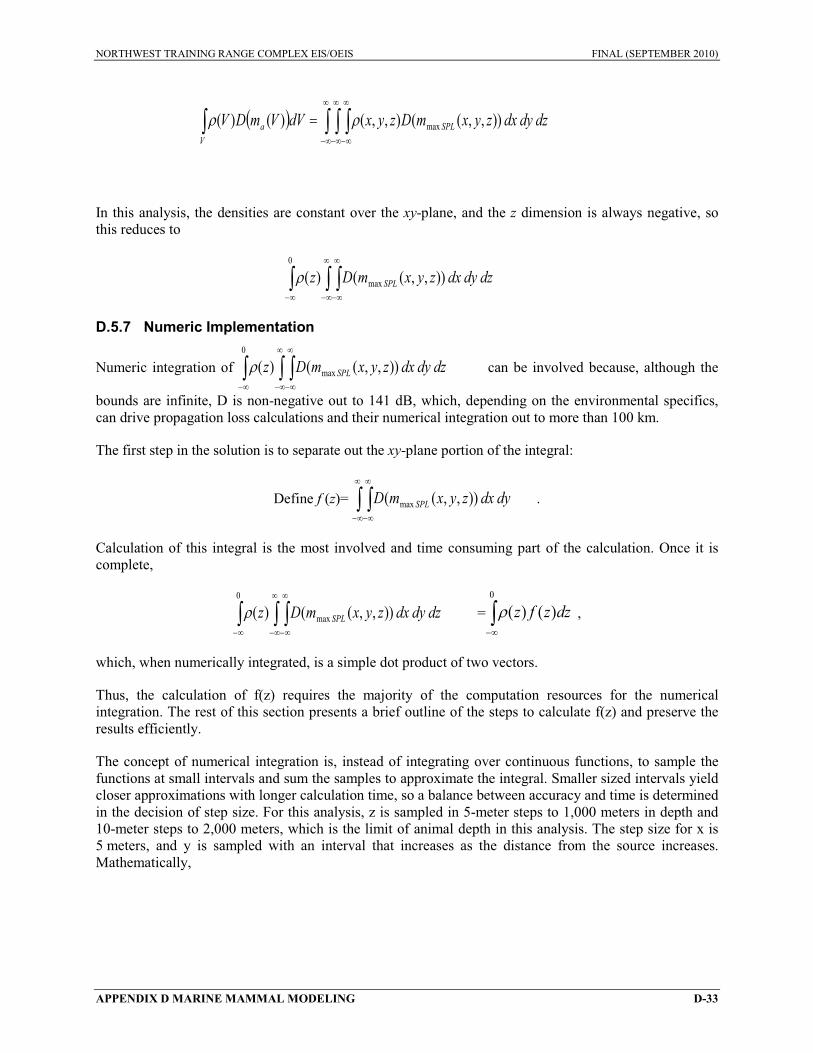
NORTHWEST TRAINING RANGE COMPLEX EIS/OEIS FINAL (SEPTEMBER 2010)
APPENDIX D MARINE MAMMAL MODELING D-33
( )∫ ∫ ∫ ∫∞
∞−
∞
∞−
∞
∞−
=V
SPLa dzdydxzyxmDzyxdVVmDV )),,((),,()()( maxρρ
In this analysis, the densities are constant over the xy-plane, and the z dimension is always negative, so this reduces to
∫ ∫ ∫∞−
∞
∞−
∞
∞−
0
max )),,(()( dzdydxzyxmDz SPLρ
D.5.7 Numeric Implementation
Numeric integration of ∫ ∫ ∫∞−
∞
∞−
∞
∞−
0
max )),,(()( dzdydxzyxmDz SPLρ can be involved because, although the
bounds are infinite, D is non-negative out to 141 dB, which, depending on the environmental specifics, can drive propagation loss calculations and their numerical integration out to more than 100 km.
The first step in the solution is to separate out the xy-plane portion of the integral:
Define f (z)= ∫ ∫∞
∞−
∞
∞−
dydxzyxmD SPL )),,(( max .
Calculation of this integral is the most involved and time consuming part of the calculation. Once it is complete,
∫ ∫ ∫∞−
∞
∞−
∞
∞−
0
max )),,(()( dzdydxzyxmDz SPLρ = ∫∞−
0
)()( dzzfzρ ,
which, when numerically integrated, is a simple dot product of two vectors.
Thus, the calculation of f(z) requires the majority of the computation resources for the numerical integration. The rest of this section presents a brief outline of the steps to calculate f(z) and preserve the results efficiently.
The concept of numerical integration is, instead of integrating over continuous functions, to sample the functions at small intervals and sum the samples to approximate the integral. Smaller sized intervals yield closer approximations with longer calculation time, so a balance between accuracy and time is determined in the decision of step size. For this analysis, z is sampled in 5-meter steps to 1,000 meters in depth and 10-meter steps to 2,000 meters, which is the limit of animal depth in this analysis. The step size for x is 5 meters, and y is sampled with an interval that increases as the distance from the source increases. Mathematically,

NORTHWEST TRAINING RANGE COMPLEX EIS/OEIS FINAL (SEPTEMBER 2010)
APPENDIX D MARINE MAMMAL MODELING D-34
{ }{ }
[ ]⎭⎬⎫
⎩⎨⎧
⎥⎦
⎤⎢⎣
⎡∗±+∗±∗±=∈
±±=∈=∈
∑=
j
i
iYy
kXxZz
0
100 )005.1(5,...,)005.1()005.1(5,)005.1(5,0
5,...,5,02000,...,1010,1000,...5,0
for integers k, j, which depend on the propagation distance for the source. For this analysis, k = 20,000 and j = 600.
With these steps, ∫ ∫∞
∞−
∞
∞−
= dxdyzyxmDzf SPL )),,(()( 0max0 is approximated as
∑∑∈ ∈
ΔΔYz Xx
SPL yxzyxmD )),,(( 0max
where X,Y are defined as above.
This calculation must be repeated for each Zz ∈0 , to build the discrete function f(z).
With the calculation of f(z) complete, the integral of its product with )(zρ must be calculated to complete evaluation of
∫∫ ∫ ∫∞−
∞
∞−
∞
∞−
∞
∞−
=0
max )()()),,(()( dzzfzdxdydzzyxmDz SPL ρρ
Since f(z) is discrete, and )(zρ can be readily made discrete, ∫∞−
0
)()( dzzfzρ is approximated numerically
as ∑∈Zz
zfz )()(ρ , a dot product.
D.5.8 Preserving Calculations for Future UseCalculating f(z) is the most time-consuming part of the numerical integration, but the most time-consuming portion of the entire process is calculating ),,(max zyxm SPL over the area range required for the cutoff value (120 dB). The calculations usually require propagation estimates out to over 100 km, and those estimates, with the beam pattern, are used to construct a sound field that extends 200 km x 200 km—40,000 sq km, with a calculation at the steps for every value of X and Y, defined above. This is repeated for each depth, to a maximum of 2,000 meters.
Saving the entire SPLmmax for each z is unrealistic, requiring great amounts of time and disk space. Instead, the different levels in the range of SPLmmax are sorted into 0.5 dB wide bins; the volume of water at each bin level is taken from SPLmmax , and associated with its bin. Saving this, the amount of water ensonified at each level, at a 0.5 dB resolution, preserves the ensonification information without using the space and time required to save SPLmmax itself. Practically, this is a histogram of occurrence of level at

NORTHWEST TRAINING RANGE COMPLEX EIS/OEIS FINAL (SEPTEMBER 2010)
APPENDIX D MARINE MAMMAL MODELING D-35
each depth, with 0.5 dB bins. Mathematically, this is simply defining the discrete functions )(LVz , where
{ }aL 5.= for every positive integer a, and for all Zz ∈ . These functions, or histograms, are saved for future work. The information lost by saving only the histograms is where in space the different levels occur, although how often they occur is saved. But the thresholds (dose response curves) are purely a function of level, not location, so this information is sufficient to calculate f(z).
Applying the dose function to the histograms is a dot product:
∑∈
≈1
0)()(
LzVD
l
ll ∫ ∫∞
∞−
∞
∞−
dxdyzyxmD SPL )),,(( 0max
So, once the histograms are saved, neither ),,(max zyxm SPL nor f(z) must be recalculated to generate
∫ ∫ ∫∞−
∞
∞−
∞
∞−
0
max )),,(()( dxdydzzyxmDz SPLρ for a new threshold function.
For the interested reader, the following section includes an in-depth discussion of the method, software, and other details of the f(z) calculation.
D.5.9 Software DetailThe risk function metric uses the cumulative normal probability distribution to determine the probability that a population of animals is affected by a given SPL. The probability distribution is defined by a low cutoff level (below which the species is not affected), a 50 percent effect level, and a steepness factor. The acoustic quantity of interest is the maximum SPL experienced over multiple pings in a range-independent environment. The procedure for calculating the impact volume at a given depth is relatively simple. In brief, given the SPL of the source and the transmission loss (TL) curve, the received SPL is calculated on a volumetric grid. For a given depth, volume associated with each SPL interval is calculated. Then, this volume is multiplied by the probability that a population of animals will be affected by that SPL. This gives the impact volume for that depth, which can be multiplied by the animal densities at that depth, to obtain the number of animals affected at that depth. The process repeats for each depth to construct the impact volume as a function of depth. It is important to note that the probabilities associated with acoustic modeling do not represent an individual’s probability of responding; they identify the proportion of an exposed population (as represented by an evenly distributed density of marine mammals per unit area) that is likely to respond to an exposure.
The case of a single emission of sonar energy, one ping, illustrates the computational process in more detail. First, the SPLs are segregated into a sequence of bins that cover the range encountered in the area. The SPL are used to define a volumetric grid of the local sound field. The impact volume for each depth is calculated as follows: for each depth in the volumetric grid, the SPL at each xy-plane grid point is calculated using the SPL of the source, the TL curve, the horizontal beam pattern of the source, and the vertical beam patterns of the source. The SPLs in this grid become the bins in the volume histogram.Figure D-14 shows a volume histogram for a low-power sonar. Level bins are 0.5 dB in width and the depth is 50 meters in an environment with water depth of 100 meters. The oscillatory structure at very low levels is due the flattening of the TL curve at long distances from the source, which magnifies the fluctuations of the TL as a function of range. The “expected” impact volume for a given level at a given depth is calculated by multiplying the volume in each level bin by the dose response probability function at that level. Total expected impact volume for a given depth is the sum of these “expected” volumes.Figure D-5 is an example of the impact volume as a function of depth at a water depth of 100 meters.

NORTHWEST TRAINING RANGE COMPLEX EIS/OEIS FINAL (SEPTEMBER 2010)
APPENDIX D MARINE MAMMAL MODELING D-36
FFigure D-14. Example of a Volume His togram
Figure D-15. Example of the Dependence of Impact Volume on Depth
The volumetric grid covers the waters in and around the area of sonar operation. The grid for this analysis has a uniform spacing of 5 meters in the x-coordinate and a slowly expanding spacing in the y-coordinate that starts with 5 meters spacing at the origin. The growth of the grid size along the y-axis is a geometric series where each successive grid size is obtained from the previous by multiplying it by 1 + Ry, where Ryis the y-axis growth factor. The nth grid size is related to the first grid size by multiplying by (1 + Ry)(n-1). For an initial grid size of 5 meters and a growth factor of 0.005, the 100th grid increment is 8.19 meters. The constant spacing in the x-coordinate allows greater accuracy as the source moves along the x-axis. The slowly increasing spacing in y reduces computation time, while maintaining accuracy, by taking advantage of the fact that TL changes more slowly at longer distances from the source. The x-and y-coordinates extend from –Rmax to +Rmax, where Rmax is the maximum range used in the TL calculations. The z direction uses a uniform spacing of 5 meters down to 1,000 meters and 10 meters from 1,000 to 2,000 meters. This is the same depth mesh used for the effective energy metric as described above. The depth mesh does not extend below 2,000 meters, on the assumption that animals of interest are not found below this depth.
0
5,000,000
10,000,000
15,000,000
20,000,000
25,000,000
30,000,000
35,000,000
116
119
122
125
128
131
134
137
140
143
146
149
152
155
158
161
164
Level (dB)
Volu
me
(m3 )
0
10,000
20,000
30,000
40,000
50,000
60,000
0 20 40 60 80 100
Depth (m)
Impa
ct V
olum
e (m
3 )

NORTHWEST TRAINING RANGE COMPLEX EIS/OEIS FINAL (SEPTEMBER 2010)
APPENDIX D MARINE MAMMAL MODELING D-37
The next three figures indicate how the accuracy of the calculation of impact volume depends on the parameters used to generate the mesh in the horizontal plane. Figure D-16 shows the relative change of impact volume for one ping as a function of the grid size used for the x-axis. The y-axis grid size is fixed at 5 meters and the y-axis growth factor is 0, i.e., uniform spacing. The impact volume for a 5-meter grid size is the reference. For grid sizes between 2.5 and 7.5 meters, the change is less than 0.1%. A grid size of 5 meters for the x-axis is used in the calculations. Figure D-17 shows the relative change of impact volume for one ping as a function of the grid size used for the y-axis. The x-axis grid size is fixed at 5 meters and the y-axis growth factor is 0. The impact volume for a 5 meters grid size is the reference. This figure is very similar to that for the x-axis grid size. For grid sizes between 2.5 and 7.5 meters, the change is less than 0.1%. A grid size of 5 meters is used for the y-axis in our calculations. Figure D-18 shows the relative change of impact volume for one ping as a function of the y-axis growth factor. The x-axis grid size is fixed at 5 meters and the initial y-axis grid size is 5 meters. The impact volume for a growth factor of 0 is the reference. For growth factors from 0 to 0.01, the change is less than 0.1%. A growth factor of 0.005 is used in the calculations.
FFigure D-16. Change of Impact Volume as a Function of x-axis Grid Size
Figure D-17. Change of Impact Volume as a Function of y-axis Grid Size
-0.2%
-0.1%
0.0%
0.1%
0 2 4 6 8 10
Grid Size (m)
Perc
enta
ge C
hang
e
-0.2%
-0.1%
0.0%
0.1%
0 2 4 6 8 10
Grid Size (m)
Perc
enta
ge C
hang
e

NORTHWEST TRAINING RANGE COMPLEX EIS/OEIS FINAL (SEPTEMBER 2010)
APPENDIX D MARINE MAMMAL MODELING D-38
FFigure D-18. Change of Impact Volume as a Function of y-axis Growth Fac tor
Another factor influencing the accuracy of the calculation of impact volumes is the size of the bins used for SPL. The SPL bins extend from 100 dB (far lower than required) up to 300 dB (much higher than that expected for any sonar system). Figure D-19 shows the relative change of impact volume for one ping as a function of the bin width. The x-axis grid size is fixed at 5 meters the initial y-axis grid size is 5 meters, and the y-axis growth factor is 0.005. The impact volume for a bin size of 0.5 dB is the reference. For bin widths from 0.25 dB to 1.00 dB, the change is about 0.1%. A bin width of 0.5 is used in our calculations.
Figure D-19. Change of Impact Volume as a Function of Bin Width
The process of obtaining the maximum SPL at each grid point in the volumetric grid is straightforward. The active sonar starts at the origin and moves at constant speed along the positive x-axis emitting a burst of energy, a ping, at regularly spaced intervals. For each ping, the distance and horizontal angle connecting the sonar to each grid point is computed. Calculating the TL from the source to a grid point has several steps. The TL is made up of the sum of many eigenrays connecting the source to the grid point. The beam pattern of the source is applied to the eigenrays based on the angle at which they leave the source. After summing the vertically beamformed eigenrays on the range mesh used for the TL calculation, the vertically beamformed TL for the distance from the sonar to the grid point is derived by interpolation. Next, the horizontal beam pattern of the source is applied using the horizontal angle
-0.1%
0.0%
0.1%
0.000 0.002 0.004 0.006 0.008 0.010
Y Axis Growth Factor
Perc
enta
ge C
hang
e
-0.1%
0.0%
0.1%
0.2%
0.2 0.4 0.6 0.8 1
Bin Width (dB)
Perc
enta
ge C
hang
e
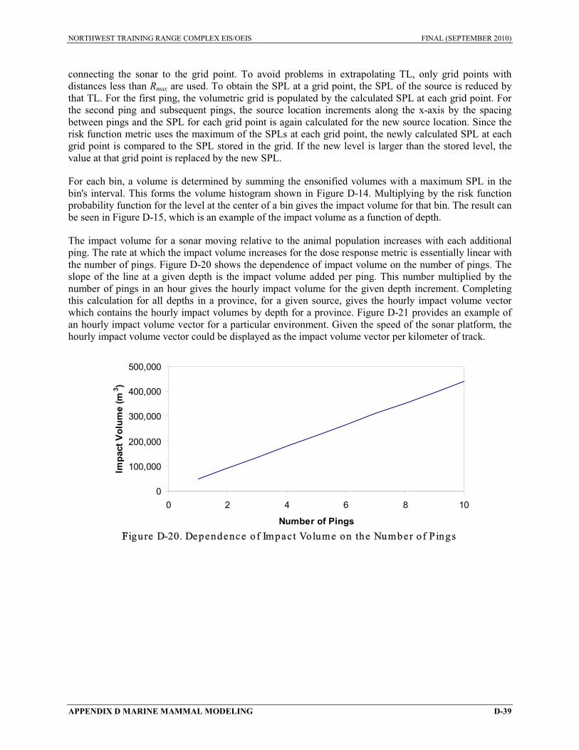
NORTHWEST TRAINING RANGE COMPLEX EIS/OEIS FINAL (SEPTEMBER 2010)
APPENDIX D MARINE MAMMAL MODELING D-39
connecting the sonar to the grid point. To avoid problems in extrapolating TL, only grid points with distances less than Rmax are used. To obtain the SPL at a grid point, the SPL of the source is reduced by that TL. For the first ping, the volumetric grid is populated by the calculated SPL at each grid point. For the second ping and subsequent pings, the source location increments along the x-axis by the spacing between pings and the SPL for each grid point is again calculated for the new source location. Since the risk function metric uses the maximum of the SPLs at each grid point, the newly calculated SPL at each grid point is compared to the SPL stored in the grid. If the new level is larger than the stored level, the value at that grid point is replaced by the new SPL.
For each bin, a volume is determined by summing the ensonified volumes with a maximum SPL in the bin's interval. This forms the volume histogram shown in Figure D-14. Multiplying by the risk function probability function for the level at the center of a bin gives the impact volume for that bin. The result can be seen in Figure D-15, which is an example of the impact volume as a function of depth.
The impact volume for a sonar moving relative to the animal population increases with each additional ping. The rate at which the impact volume increases for the dose response metric is essentially linear with the number of pings. Figure D-20 shows the dependence of impact volume on the number of pings. The slope of the line at a given depth is the impact volume added per ping. This number multiplied by the number of pings in an hour gives the hourly impact volume for the given depth increment. Completing this calculation for all depths in a province, for a given source, gives the hourly impact volume vector which contains the hourly impact volumes by depth for a province. Figure D-21 provides an example of an hourly impact volume vector for a particular environment. Given the speed of the sonar platform, the hourly impact volume vector could be displayed as the impact volume vector per kilometer of track.
FFigure D-20. Dependence of Impact Volume on the Number of P ings
0
100,000
200,000
300,000
400,000
500,000
0 2 4 6 8 10
Number of Pings
Impa
ct V
olum
e (m
3 )

NORTHWEST TRAINING RANGE COMPLEX EIS/OEIS FINAL (SEPTEMBER 2010)
APPENDIX D MARINE MAMMAL MODELING D-40
FFigure D-21. Example of an Hourly Impact Volume Vector
D.6 EXPOSURE ESTIMATES
Densities are usually reported by marine biologists as animals per square kilometer (km2), which is an area metric. This gives an estimate of the number of animals below the surface in a certain area, but does not provide any information about their distribution in depth. The impact volume vector (see subsection D.4.3) specifies the volume of water ensonified above the specified threshold in each depth interval. A corresponding animal density for each of those depth intervals is required to compute the expected value of the number of exposures. The two-dimensional area densities do not contain this information, so three-dimensional densities must be constructed by using animal depth distributions to extrapolate the density at each depth. The required depth distributions are presented in the biology subsection.
The following sperm whale example demonstrates the methodology used to create a three-dimensional density by merging the area densities with the depth distributions. The sperm whale surface density is 0.0117 whales per km2. From the depth distribution report, “depth distribution for sperm whales based on information in the Amano paper is: 31% in 0-10 m, 8% in 10-200 m, 9% in 201-400 m, 9% in 401-600 m, 9% in 601-800 m and 34% in >800 m.” So the sperm whale density at 0-10 m is 0.0117*0.31/0.01 = 0.3627 per cubic km, at 10-200 m is 0.0117*0.08/0.19 = 0.004926 per cubic km, and so forth.
In general, the impact volume vector samples depth in finer detail than given by the depth distribution data. When this is the case, the densities are apportioned uniformly over the appropriate intervals. For example, suppose the impact volume vector provides volumes for the intervals 0-10 meters, 10-50 meters, and 50-200 meters. Then for the depth-distributed densities discussed in the preceding paragraph,
• 0.3627 whales per cubic km is used for 0-10 meters,
• 0.004926 whales per cubic km is used for 10-50 meters, and
• 0.004926 whales per cubic km is used for 50-200 meters.
Once depth-varying, three-dimensional densities are specified for each species type, with the same depth intervals and the ensonified volume vector, the density calculations are finished. The expected number of ensonified animals within each depth interval is the ensonified volume at that interval multiplied by the volume density at that interval and this can be obtained as the dot product of the ensonified volume and animal density vectors.
-100.00
-80.00
-60.00
-40.00
-20.00
0.00
0.00 30.00 60.00 90.00 120.00 150.00 180.00
Impact Volume (109 m3)
Dept
h (m
)

NORTHWEST TRAINING RANGE COMPLEX EIS/OEIS FINAL (SEPTEMBER 2010)
APPENDIX D MARINE MAMMAL MODELING D-41
Since the ensonified volume vector is the ensonified volume per unit operation (i.e., per hour, per sonobuoy, etc.), the final exposure count for each species is the unit operation exposure count multiplied by the number of units (hours, sonobuoys, etc).
DD.7 P OST ACOUSTIC MODELING ANALYSIS
The acoustic modeling results include additional analysis to account for land mass, multiple ships, and number of animals that could be exposed. Specifically, post modeling analysis is designed to consider:
Acoustic footprints for sonar sources must account for land masses.
Acoustic modeling should account for the maximum number of individuals of a species that could potentially be exposed to sonar within the course of 1 day or a discreet continuous sonar event if less than 24 hours.
When modeling the effect of sound projectors in the water, the ideal task presents modelers with complete a priori knowledge of the location of the source(s) and transmission patterns during the times of interest. In these cases, calculation inputs include the details of source path, proximity of shoreline, high-resolution density estimates, and other details of the scenario. However, in the NWTRC, there are sound-producing events for which the source locations and transmission patterns are unknown, but still require analysis to predict effects. For these cases, a more general modeling approach is required: “We will be operating somewhere in this large area for X minutes. What are the potential effects on average?”
Modeling these general scenarios requires a statistical approach to incorporate the scenario nuances into harassment calculations. For example, one may ask: “If an animal receives 130 dB SPL when the source passes at CPA on Tuesday morning, how do we know it does not receive a higher level on Tuesday afternoon?” This question cannot be answered without knowing the path of the source (and several other facts). Because the path of the source is unknown, the number of an individual’s re-exposures cannot be calculated directly. But it can, on average, be accounted for by making appropriate assumptions.
Table D-11 lists unknowns created by uncertainty about the specifics of a future proposed action, the portion of the calculation to which they are relevant, and the assumption that allows the effect to be computed without the detailed information:
Table D-11. Unknowns an d As s umptions
Unknowns Relevance Assumption
Path of source(esp. with respect to animals)
Ambiguity of multiple exposures, Local population: upper bound of harassments
Most conservative case: sources can be anywhere within range
Source locations Ambiguity of multiple exposures, land shadow
Equal distribution of action in each range
Direction of sonar transmission
Land shadow Equal probability of pointing any direction
The following sections discuss two topics that require action details, and describe how the modeling calculations used the general knowledge and assumptions to overcome the future-action uncertainty with respect to re-exposure of animals, and land shadow.

NORTHWEST TRAINING RANGE COMPLEX EIS/OEIS FINAL (SEPTEMBER 2010)
APPENDIX D MARINE MAMMAL MODELING D-42
D.7.1 Multiple Exposures in General Modeling ScenarioConsider the following hypothetical scenario. A box is painted on the surface of a well-studied ocean environment with well-known propagation. A sonar-source and 100 whales are inserted into that box and a curtain is drawn. What will happen? The details of what will happen behind the curtain are unknown, but the existing knowledge, and general assumptions, can allow for a calculation of average affects.
For the first period of time, the source is traveling in a straight line and pinging at a given rate. In this time, it is known how many animals, on average, receive their max SPLs from each ping. As long as the source travels in a straight line, this calculation is valid. However, after an undetermined amount of time, the source will change course to a new and unknown heading.
If the source changes direction 180 degrees and travels back through the same swath of water, all the animals the source passes at CPA before the next course change have already been exposed to what will be their maximum SPL, so the population is not “fresh.” If the direction does not change, only new animals will receive what will be their maximum SPL from that source (though most have received sound from it), so the population is completely “fresh.” Most source headings lead to a population of a mixed “freshness,” varying by course direction. Since the route and position of the source over time are unknown, the freshness of the population at CPA with the source is unknown. This ambiguity continues through the remainder of the exercise.
What is known? The source and, in general, the animals remain in the vicinity of the range. Thus, if the farthest range to a possible effect from the source is X km, no animals farther than X km outside of the operating area (OPAREA) can be harassed. The intersection of this area with a given animal’s habitat multiplied by the density of that animal in its habitat represents the maximum number of animals that can be harassed by activity in that OPAREA, which shall be defined as “the local population.” Two details: first, this maximum should be adjusted down if a risk function is being used, because not 100% of animals within X km of the OPAREA border will be harassed. Second, it should be adjusted up to account for animal motion in and out of the area.
The ambiguity of population freshness throughout the exercise means that multiple exposures cannot be calculated for any individual animal. It must be dealt with generally at the population level.
D.7.1.1 Solution to Ambiguity of Multiple Exposures in the General Modeling Scenario
At any given time, the population has received a maximum SPL (possibly zero) that indicates the probability of harassment in the exercise. This probability indicates the expected value of the number of harassments. For example, if a population receives a level that indicates 50% probability of harassment, it contributes 0.5 to the sum of the expected number of harassments. If it is passed later with a higher level that indicates a 70% chance of harassment, its contribution increases to 0.7. Let the expected value of harassments at a given time be defined as “the harassed population” and the difference between the local population (as defined above) and the harassed population be defined as “the unharassed population.” As the exercise progresses, the harassed population will never decrease and the unharassed population will never increase. It is important to note that the probabilities associated with acoustic modeling do not represent an individual’s probability of responding; they identify the proportion of an exposed population (as represented by an evenly distributed density of marine mammals per unit area) that is likely to respond to an exposure.
The unharassed population represents the number of animals statistically “available” for harassment. Since we do not know where the source is, or where these animals are, we assume an average (uniform) distribution of the unharassed population over the area of interest. The densities of unharassed animals are lower than the total population density because some animals in the local population are in the harassed population.

NORTHWEST TRAINING RANGE COMPLEX EIS/OEIS FINAL (SEPTEMBER 2010)
APPENDIX D MARINE MAMMAL MODELING D-43
Density relates linearly to expected harassments. If action A in an area with a density of 2 animals per km2 produces 100 expected harassments, then action A in an area with 1 animal per km2 produces 50 expected harassments. The modeling produces the number of expected harassments per ping starting with 100% of the population unharassed. The next ping will produce slightly fewer harassments because the pool of unharassed animals is slightly less.
For example, consider the case where 1 animal is harassed per ping when the local population is 100, 100% of which are initially unharassed. After the first ping, 99 animals are unharassed, so the number of animals harassed during the second ping are
99.0)99(.1100991 ==⎟
⎠⎞
⎜⎝⎛ animals
and so on for the subsequent pings.
A closed form function for this process can be derived as follows.
Define =H number of animals harassed per ping with 100% unharassed population. H is calculated by determining the expected harassments for a source moving in a straight line for the duration of the exercise and dividing by the number of pings in the exercise (Figure D-22).
Figure D-22. Proces s of Calcula ting H
The total unharassed population is then calculated by iteration. Each ping affects the un-harassed population left after all previous pings:
Define =nP unharassed population after ping n
=0P local population
H =∫ ∫ ∫ dxdydzzyxLDz )),,(()(ρ /Npings

NORTHWEST TRAINING RANGE COMPLEX EIS/OEIS FINAL (SEPTEMBER 2010)
APPENDIX D MARINE MAMMAL MODELING D-44
⎠
⎞⎜⎜⎝
⎛−=
⎟⎟⎠
⎞⎜⎜⎝
⎛−=
−=
−−
0
11
0
112
01
...
PP
HPP
PPHPP
HPP
nnn
Therefore,
n
nnn PHP
PHP
PHPP ⎟
⎟⎠
⎞⎜⎜⎝
⎛⎟⎟⎠
⎞⎜⎜⎝
⎛−==⎟
⎟⎠
⎞⎜⎜⎝
⎛⎟⎟⎠
⎞⎜⎜⎝
⎛−=⎟
⎟⎠
⎞⎜⎜⎝
⎛⎟⎟⎠
⎞⎜⎜⎝
⎛−= −−
00
2
02
01 1...11
Thus, the total number of harassments depends on the per-ping harassment rate in an un-harassed population, the local population size, and the number of operation hours.
D.7.1.2 Local Population: Upper Bound on Harassments
As discussed above, Navy planners have confined periods of sonar use to training areas. The size of the harassed population of animals for an action depends on animal re-exposure, so uncertainty about the precise source path creates variability in the “harassable” population. Confinement of sonar use to a sonar training area allows modelers to compute an upper bound, or worst case, for the number of harassments with respect to location uncertainty. This is done by assuming that every animal which enters the training area at any time in the exercise (and also many outside) is “harassable” and creates an upper bound on the number of harassments for the exercise. Since this is equivalent to assuming that there are sonars transmitting simultaneously from each point in the confined area throughout the action length, this greatly overestimates the harassments from an exercise.
NMFS has defined a 24-hour “refresh rate,” or the accumulated exposures over 24 hours. The Navy has determined that, in a 24-hour period, all sonar activities in the NWTRC transmit for no longer than 2 hours.
The most conservative assumption for a single ping is that it harasses the entire population within the range (a gross over-estimate). However, the total harassable population for multiple pings will be even greater since animal motion over the period in the above table can bring animals into range that otherwise would be out of the harassable population.
D.7.1.3 Animal Motion Expansion
Though animals often change course to swim in different directions, straight-line animal motion would bring the more animals into the harassment area than a “random walk” motion model. Since precise and accurate animal motion models exist more as speculation than documented fact and because the modeling requires an undisputable upper bound, calculation of the upper bound for NWTRC modeling areas uses a straight-line animal motion assumption. This is a conservative assumption.
For a circular area, the straight-line motion in any direction produces the same increase in harassable population. However, since the ranges are non-circular polygons, choosing the initial fixed direction as perpendicular to the longest diagonal produces greater results than any other direction. Thus, the product of the longest diagonal and the distance the animals move in the period of interest gives an overestimate

NORTHWEST TRAINING RANGE COMPLEX EIS/OEIS FINAL (SEPTEMBER 2010)
APPENDIX D MARINE MAMMAL MODELING D-45
of the expansion in range modeling areas due to animal motion. The NWTRC expansions use this estimate as an absolute upper bound on animal-motion expansion.
Figure D-23 illustrates an example of the overestimation, which occurs during the second arrow:
FFigure D-23. Proces s of Se tting an Upper Bound on Individua ls Pres ent in Area
It is important to recognize that the area used to calculate the harassable population, shown in Figure D-23 will, in general, be much larger than the area that will be within the ZOI of a ship for the duration of its broadcasts. For a ship moving faster than the speed of the marine animals, a better (and much smaller) estimate of the harassable population would be that within the straight line ZOI cylinder shown in Figure D-22. Using this smaller population would lead to a greater dilution of the unharassed population per ping and would greatly reduce the estimated harassments.
D.7.1.4 Risk Function Expansion
The expanded area contains the number of animals that will enter the range over the period of interest. However, an upper bound on harassments must also include animals outside the area that would be affected by a source transmitting from the area’s edge. A gross overestimation could simply assume pinging at every point on the range border throughout the exercise and would include all area with levels from a source on the closest border point greater than the risk function basement. In the case of NWTRC, this would include all area within approximately 150 km from the edge of the adjusted box. This basic method would give a crude and exaggerated upper bound, since only a tiny fraction of this out-of-range area can be ensonified above threshold for a given ping. A more refined upper bound on harassments can be found by maintaining the assumption that a sonar is transmitting from each point in the adjusted box
Random individuals and operating area Random Initial Direction: 10 intersections
Uniform Initial Direction:11 Intersections
An individual inside the adjusted box will be in the original box sometime during the period of interest.

NORTHWEST TRAINING RANGE COMPLEX EIS/OEIS FINAL (SEPTEMBER 2010)
APPENDIX D MARINE MAMMAL MODELING D-46
and calculating the expected ensonified area, which would give all animals inside the area a 100% probability of harassment, and those outside the area a varying probability, based on the risk function.
∫− )120(
0
1
))((dBL
drrLD ,
Where L is the SPL function with domain in range and range in level,
r is the range from the sonar operating area,
L-1(120 dB) is the range at which the received level drops to 120 dB, and
D is the risk function function (probability of harassment vs. Level).
At the corners of the polygon, additional area can be expressed as
[ ]
π
θπ
2
))(()120(
0
1
∫−
−dBL
rdrrLD
with D, L, and r as above, and
θ the inner angle of the polygon corner, in radians.
For the risk function and transmission loss of the NWTRC, this method adds an area equivalent by expanding the boundaries of the adjusted box by 4 km. The resulting shape, the adjusted box with a boundary expansion of 4 km, does not possess special meaning for the problem. But the number of individuals contained by that shape, is the harassable population and an absolute upper bound on possible harassments for that operation.
The following plots (Figure D-24) illustrate the growth of area for the sample case above. The shapes of the boxes are unimportant. The area after the final expansion, though, gives an upper bound on the “harassable,” or initially unharassed population which could be affected by operations.
FFigure D-24. Proces s of Expanding Area to Crea te Upper Bound of Haras s ments
Expanded for Dose ResponseExpanded for Animal MotionOriginal Area

NORTHWEST TRAINING RANGE COMPLEX EIS/OEIS FINAL (SEPTEMBER 2010)
APPENDIX D MARINE MAMMAL MODELING D-47
D.7.1.5 Example Case
Consider a sample case from the NWTRC General Area. For the most powerful source, the 53C, the expected winter rate of harassment for short-finned pilot whales is approximately 0.00022128 harassments per ping. The exercise will transmit sonar pings for 2 hours in a 24-hour period as consistent with NWTRC planned use, with 120 pings per minute, a total of 120*2=240 pings in a 24-hour period.
The NWTRC General Area has an area of approximately 422,265 km2 and a diagonal of 1,053 km. Adjusting this with straight-line (upper bound) animal motion of 5.5 km per hour for 2 hours, animal motion adds 1,053*5.5*2= 11,583 km2 to the area. Using the risk function to calculate the expected range outside the speed of advance adds another 11,295 km2, bringing the total upper-bound of the affected area to 445,143 km2.
For this analysis, short-finned pilot whales have an average winter density of 0.00005 animals per km2, so the upper bound number short-finned pilot whales that can be affected by 53C activity in the NWTRCduring a 24-hour period is 445,143 *0.00005=22.3 whales.
In the first ping, 0.00022128 short-finned pilot whales will be harassed. With the second ping,
780.000221273.22
0.000221283.220.00022128 =⎟⎠⎞
⎜⎝⎛ −
short-finned pilot whales will be harassed.
Using the formula derived above, after 2 hours of continuous operation, the remaining unharassed
population is 22.253.22
.0002212813.221240240
00240 ≈⎟⎟
⎠
⎞⎜⎜⎝
⎛⎟⎠⎞
⎜⎝⎛−=⎟
⎟⎠
⎞⎜⎜⎝
⎛⎟⎟⎠
⎞⎜⎜⎝
⎛−=
PhPP
So the harassed population will be 22.3-22.25 = 0.05 animals.
Contrast this with linear accumulation of harassments without consideration of the local population and the dilution of the unharassed population:
Harassments = 0.00022128 * 240=0.053 animals
The difference in harassments is very small, as a percentage of total harassments, because the size of the NWTRC implies a large “harassable” population relative to the harassment per ping of the 53C. In cases where the harassable population is not as large, with respect to the per ping harassments, the difference in harassments between linear accumulation and density dilution is more pronounced.
D.7.2 Land ShadowThe risk function considers harassment possible if the animal population receives 120 dB SPL, or above.In the open ocean of the NWTRC, this can occur as far away as 150 km, so over a large “effect” area, sonar sound could, but does not necessarily, harass an animal. The harassment calculations for a general modeling case must assume that this effect area covers only water fully populated with animals, but in some portions of the NWTRC, land partially encroaches on the area, obstructing sound propagation.
As discussed in the introduction of this section, Navy planners do not know the exact location and transmission direction of the sonars at future times. These factors however, completely determine the interference of the land with the sound, or “land shadow,” so a general modeling approach does not have enough information to compute the land shadow effects directly. However, modelers can predict the reduction in harassments at any point due to land shadow for different pointing directions and use

NORTHWEST TRAINING RANGE COMPLEX EIS/OEIS FINAL (SEPTEMBER 2010)
APPENDIX D MARINE MAMMAL MODELING D-48
expected probability distribution of activity to calculate the average land shadow for operations in each range.
For each of the coastal points that are within 150 km of the grid, the azimuth and distance is computed. In the computation, only the minimum range at each azimuth is computed. The minimum range compared with azimuth for the sample point is shown in Figure D-25.
FFigure D-25. The neares t poin t a t each azimuth (with 1o s pacing) to a s ample grid poin t (red circle ) is s hown by the green lines .
Now, the average of the distances to shore, along with the angular profile of land is computed (by summing the unique azimuths that intersect the coast) for each grid point. The values are then used to compute the land shadow for the grid points.
D.7.2.1 Computing the Land Shadow Effect at Each Grid Point
The effect of land shadow is computed by determining the levels, and thus the distances from the sources, that the harassments occur. Table D-12 and Figure D-26 give a mathematical extrapolation of the distances and levels at which harassments occur, with average propagation in the NWTRC.

NORTHWEST TRAINING RANGE COMPLEX EIS/OEIS FINAL (SEPTEMBER 2010)
APPENDIX D MARINE MAMMAL MODELING D-49
TTable D-12. Beh aviora l Haras s ments a t each Rece ived Level Band from 53C
Received Level(dB SPL)
Distance at which Levels Occur in NWTRC
Percent of Behavioral HarassmentsOccurring at Given Levels
Below 140 51 km - 130 km < 1%
140<Level<150 25 km – 51 km 2%
150<Level<160 10 km – 25 km 18%
160<Level<170 3 km – 10 km 43%
170<Level<180 560 m – 3 km 28%
Above 180 dB 0 m – 560 m < 9%
Figure D-26. Approximate Percentage of Behaviora l Haras s ments for Every 5 Degree Band of Received Leve l from the 53C
With the data used to produce the previous figure, the average effect reduction across season for a sound path blocked by land can be calculated. For the 53C, since approximately 81% of harassments occur within 10 km of the source (Figure D-27), a sound path blocked by land at 10 km will, on average, cause approximately 81% of the effect of an unblocked path.
120 125 130 135 140 145 150 155 160 165 170 175 180 1850
5
10
15
Received Level (dB)
Per
cent
age
of H
aras
smen
ts

NORTHWEST TRAINING RANGE COMPLEX EIS/OEIS FINAL (SEPTEMBER 2010)
APPENDIX D MARINE MAMMAL MODELING D-50
FFigure D-27. Average Percentage of Haras s ments OccurringWithin a Given Dis tance
As described above, the mapping process determines the angular profile of and distance to the coastline(s) from each grid point. The distance, then, determines the reduction due to land shadow when the sonar is pointed in that direction. The angular profile, then, determines the probability that the sonar is pointed at the coast.
Define θn = angular profile of coastline at point n in radians
Define rn = mean distance to shoreline
Define A(r) = average effect adjustment factor for sound blocked at distance r
The land shadow at point n can be approximated by A(rn)θn/(2π). For illustration, Figures D-28 and D-29give the land shadow reduction factor at each point in each range area for the 53C. The white portions of these figures indicate the areas outside the range and the blue lines indicate the coastline. The color plots inside the ranges give the land shadow factor at each point. The average land shadow factor from the 53C for the NWTRC is 0.9992 and for the special case of harbor porpoises is 0.9116; the reduction in effect is 0.0008% for the former and 8.84% for the latter. For the other, lower-power sources, this reduction is negligible.
0 5 10 15 20 25 30 35 400
10
20
30
40
50
60
70
80
90
100
Distance from Source (km)
Per
cent
age
of H
aras
smen
ts

NORTHWEST TRAINING RANGE COMPLEX EIS/OEIS FINAL (SEPTEMBER 2010)
APPENDIX D MARINE MAMMAL MODELING D-51
FFigure D-28. Depiction of Land Shadow over Warning Area 237
Figure D-29. Depiction of Land Shadow over NWTRC

NORTHWEST TRAINING RANGE COMPLEX EIS/OEIS FINAL (SEPTEMBER 2010)
APPENDIX D MARINE MAMMAL MODELING D-52
DD.8 REFERENCES
Arons, A.B. (1954). “Underwater Explosion Shock Wave Parameters at Large Distances from the Charge,” J. Acoust. Soc. Am. 26, 343.
Bartberger, C.L. (1965). “Lecture Notes on Underwater Acoustics,” NADC Report NADC=WR-6509, Naval Air Development Center Technical Report, Johnsville, PA, 17 May (AD 468 869) (UNCLASSIFIED).
Christian, E.A. and J.B. Gaspin, (1974). Swimmer Safe Standoffs from Underwater Explosions,” NSAP Project PHP-11-73, Naval Ordnance Laboratory, Report NOLX-89, 1 July (UNCLASSIFIED).
Department of the Navy (1998), “Final Environmental Impact Statement, Shock Testing the SEAWOLF Submarine,” U.S. Department of the Navy, Southern Division, Naval Facilities Engineering Command, North Charleston, SC, 637 p.
Department of the Navy (2001), “Final Environmental Impact Statement, Shock Trial of the WINSTON S. CHURCHILL (DDG 81),” U.S. Department of the Navy, NAVSEA, 597 p.
Goertner, J.F. (1982), “Prediction of Underwater Explosion Safe Ranges for Sea Mammals,” NSWC TR 82-188, Naval Surface Weapons Center, Dahlgren, VA.
Keenan, R.E., Denise Brown, Emily McCarthy, Henry Weinberg, and Frank Aidala (2000). “Software Design Description for the Comprehensive Acoustic System Simulation (CASS Version 3.0) with the Gaussian Ray Bundle Model (GRAB Version 2.0)”, NUWC-NPT Technical Document 11,231, Naval Undersea Warfare Center Division, Newport, RI, 1 June (UNCLASSIFIED).
McGrath, J.R. (1971). “Scaling Laws for Underwater Exploding Wires,” J. Acoust. Soc. Am. 50, 1030-1033 (UNCLASSIFIED).
Urick, R.J. (1983). Principles of Underwater Sound for Engineers, McGraw-Hill, NY (first edition: 1967, second edition: 1975) (UNCLASSIFIED).
Weston, D.E. (1960). “Underwater Explosions as Acoustic Sources,” Proc. Phys. Soc. 76, 233 (UNCLASSIFIED).
Related Documents