- - D-A205 205 4-, '7~ "4 'e- es, ", JD 21knd~fi&c V i~' Sy/isqth4krtokjt 5' I-.' - ER19,37- ApfAoteIU4Ep~fl pteese:uisfizan i nliiud nHA~PR . 4~4b ' 1<kAf DIt.F$i?(ilABR n HUIA SY XTM DIVSIA AIR nrwYwUSCMMN WRIGHTP~rtUM 3AMtC~ -,OC 4E H ,d4-&

Welcome message from author
This document is posted to help you gain knowledge. Please leave a comment to let me know what you think about it! Share it to your friends and learn new things together.
Transcript
- - D-A205 205
4-,
'7~ "4 'e-
es, ", JD
21knd~fi&c V i~'
Sy/isqth4krtokjt 5'
I-.' - ER19,37-
ApfAoteIU4Ep~fl pteese:uisfizan i nliiud
nHA~PR . 4~4b ' 1<kAf DIt.F$i?(ilABR n
HUIA SY XTM DIVSIA
AIR nrwYwUSCMMN
WRIGHTP~rtUM 3AMtC~ -,OC 4E H ,d4-&

BestAvailable
Copy
UUL~fl1W
SCURITY CLASSIFICATION CF THIS PAGE
Fcom AppovedREPORT DOCUMENTATION PAGE OMSNo.0704-01M
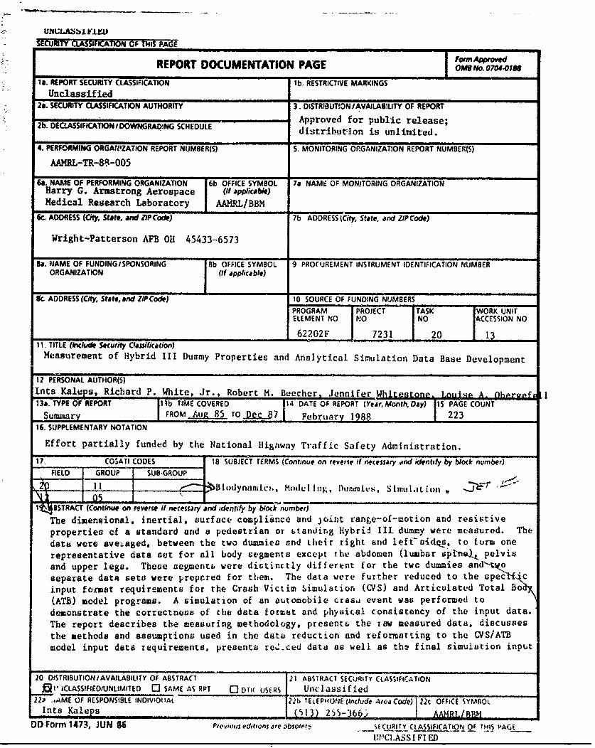
la. REPORT SECURITY CLASSIFICATION lb. RESTRICTIVE MARKINGSUnclassified
2a. SECURITY CLASSIFICATION AUTHORITY 3. DISTRIBUT!ON/AVAILABIUTY OF REPORT
Approved for public release;2b. DECLASSIFICATIONIDOWNGRADiNG SCHEDULE dpproved for iulimired." distrihut-lon is unlimited.
4. PERFORMING ORGAUIZATION REPORT NUMBER(S) S. MONITORING ORGANIZATION REPORT NUMBER(S)
AAHRL-TR-88-005
6a. NAME OF PERFORMING ORGANIZATION [6b OFFICE SYMBOL 7a NAME OF MON!TORING ORGANIZATIONHarry G. Armstrong Aerospace (If applkofIle)Medical Research Laboratory AAMRL/BBM
6c_ ADDRESS (City, State, and ZIP Code) 7b ADDRESS (City, State, and ZIP Code)
Wright-Patterson AFB OH 45433-6573
B. MAME OF FUNDING/SPONSORING Rb OFFICE' SYMBOL 9 PROCUREMENT INSTRUMENT IDENTIFICATION NUMBER
ORGANIZATION (If applicable)
Ic. ADDRESS (City, State, and ZIP Code) 10 SOURCE OF FUNDING NUMBERSELEMENT NO NO NO ACCESSION NO
62202F 7231 20 I1311. TITLE (Mchxk Security Clasjfication)
Measurement of Hybrid III Dummy Properties and Analytical Simulation Data Base Development
12 PERSONAL AUTHOR(S)Ints Kaleps, Richard P. White, Jr., Robert M. Beecher. Jennifer hitestone o A- raf13a. TYPE OF REPORT 13b TIME COVERED 14 DATE OF REPORT (Year, Month Day) 15 PAGE COUNT
Summary FROM AuR 85 TO ,_7 February 12h 22316. SUPPLEMENTARY NOTATION
Effort partially funded by the National Higaway Traffic Safety Admlnistration.
17, COSATI CODES 18 SUBJECT TERMS (Continue on reverie if necessary and identify by block number)FIELD GROUP SUB.GROUP
11 I>Blodynamtcs., Mode11i g D:nmjie h. SimulIat ion -~051 ,Tntkm* on revert if necessary and identfy by block number)
The dimensional. inertial. surface compliance and joint range-of-motion and resistiveproperties of a standard and a pedestrian or Ltanding Hybrid IIL dummy were measured. Thedata were ave-aged. between the two dummies and their right and left-sides. to form one
representative data set for all body segments except the abdomen (lumbar upin e. pelvisand upper legs. These segments were distinctly different for the two dummies and-tkoseparate data sets were preperea for them. The data were further reduced to the spec . cinput format requirements for the Crash Victim Limulation (CVS) and Articulated Total Bo(ATB) model programs. A simulation of an automobile cras. event was performed todemonstrate the correctness of che data format and physical consistency of the input data.The report describes the measuring methodology. presents the raw measured data, discussesthe methods and assumptions used in the data reduction and reformatting to the CVS/ATBmodel input data requirements, presents re -ced data as well as the final simulation input
20 DISTRIBUTION /AVAILABILITY OF ABSTRACT 21 ABSTRACT SECUR)i ry CLASSIFICATIONRI"JCLASSIFIEDIUNLIMITEO 0 SAME AS RPT 0 DI( USERS Unclassified
22-" -.AME OF RESPONSILE INDIVI01AL 22b TELEPHOE (Include Arc'a Code) 22c OFFICE SYMBOLInts Kaleps (513) 2.,-366. I AAMRLI//813
DD Form 1473, JUN 86 Prevous editions ire ablolefi ,ECURITY CLASSIFiCATtON OF THIS PAGE
UIC1.ASS I FI ED
19. ABSTRACT (Contiued)
formatted data and shows graphical results from the demonstration simulations in whichresponses of the standard Hybrid MI. the standing Hybrid III and a Part 572 duiny,exposed to identical impact conditions. are compsrtd.
IPREPN2F
The york described herein was Derformed at the Harry G. Armstrong
Aerospace Medical Research Laboratory (AAMRL) and was supported by borl.
Ait Force and National Highway Trattic Satety AdMivirtration F'unding
(Interagency Agreement No. DTNH22-86-X-07477). The various tasks
necessary for the total program were performed in part by AAMRL. Systems
stesearch Laboratory. Inc. and University of Dayton Research Institute
personnel. Of the two Hybrid IIl dummies tested in this program the
standing dummy belonged to AAMRL and the seated dummy was provided by
General Motors.
'I,,
(Revibed 5/6/87)
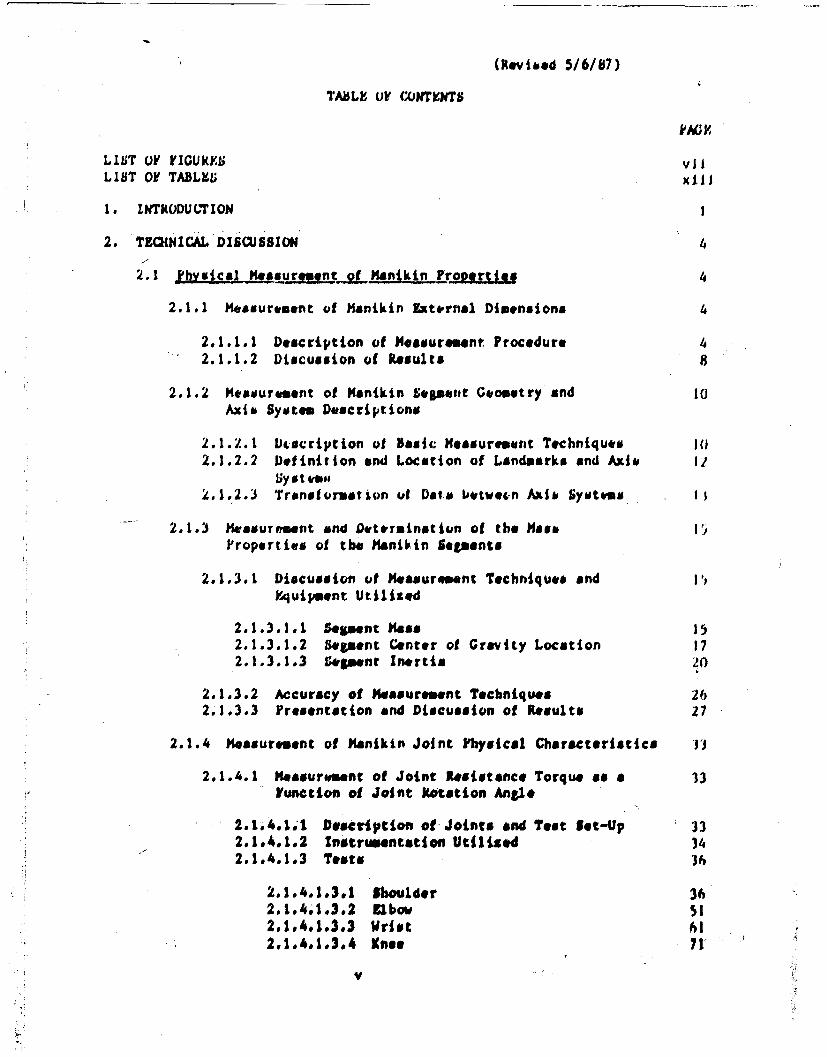
TABiLE OF' COtNTYt4TS
LIST OF VIGUiS viiLIST OF TABLES xiii
1. ZNTRODUCTION
2. TECHNICAL DISCUSSION 4
2.1 Yhysigjg ,,surment of Manikin Proverties 4
2.1.1 Measurement of Manikin htornal Dimensions 4
2.1.1.1 Description of Messurment Procedure 42.1.1.2 Discussion of Results 8
2.1.2 Measurement of Manikin Sement Geometry and 10Axib System Dscriptions
2.1.2.1 Dcription of basic Measurement Techniques t02.1.2.2 Definition and Location of Landmarks and Axi& I;
Sy at vel2.1.2.3 Transformation of Data 4etve-n Axib Systems I
2.1.3 Measurement and Determinatiun of the Me s1I
P'ropertivs of the Manikin Semtents
2.1.3.1 Discussion of Measureoment Techniques and I,Equipment Utilized
2.1.3.1.1 $ement Mass 152.1.3.1.2 Segment Center of Gravity Location 172.1.3.1.3 Segment Inertia 20
2.1.3.2 Accuracy of Measurement Techniques 26
2.1.3.3 Fresentation and Discussion of Results 27
2.1.4 Measurement of Manikin Joint Physical Characteristics V)
2.1.4.1 Measuroment of Joint Re sistance Torque as a 33function of Joint Rotation Angle
2.1.4.14 Description of Joints and Test Set-Up 332.1.4.1.2 Initrusentation Utilized 342.1.4.1.3 Teats 36
2.1.4.1.3.1 Shoulder 362.1.4.1.3.2 Elbow 512.1#4.1.3.3 Wrist 612.1.4.1.3.4 Knee 71
v
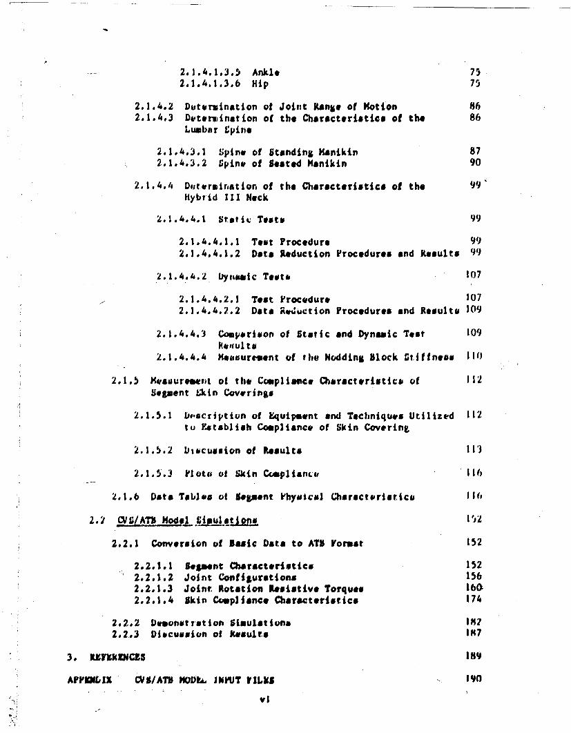
S2.1.4.1.3.5 Ankle 75
2.1.4.1.3.6 Hip 75
2.1.4.2 Dutermination ot Joint Rainge of Motion 862.1.4.3 Deterumlnatlon of the Characteristics of the 86
Lumbar Vpine
2.1.4.3.1 Spins, of Standing Manikin 872.1.4.3.2 Spine of Seated Manikin 90
2.1.4.4 Doitertration of the Characteristics of the 99Hybrid III Nock
2.1.4.4.1 Static Test& 99
2.1.4.4.1.1 Test Procedure 992.1.4.4.1.2 Data Reduction Procedures and Pesults 99
2.1.4.4.2 Dya |c Tot6 107
2.1.4.4.2.1 Test Procedure 1072.1.4.4.2.2 Data Rviuction Procedures and Reaulto 109
2.1.4.4.3 Comparison of Static and Dynamic Test 109keaul ts
2.1.4.4.4 Neasuretwnt of the Nodding block Stiffness 110
2.1.5 Meauureawrt of the Compliance Characteristic& of 112Segment kin Coverings
2.1.5.1 D.scription of Equipment and Techniques Utilized 112to Fatablish Compliance of Skin Covering
2.1.5.2 Discussion of Results 113
2.1.5.3 Plotu of Skin Complianc& 116
2.1.6 Data Table# of Sement khyoical Characteristics lib
2.2 CV S/ Am Model 1WUs}QS3,
2.2.1 Conversion of Basic Data to ATO Vorimt 152
2.2.1.1 Segment Characteristics 1522.2.1.2 Joint Configurations 1362.2.1.3 Joint Rotation Resistive Torques 1602.2.1.4 Skin Compliance Characteristics 174
2,2.2 Demonstration Simulations 1872.2.3 Discussion of Rsults 187
3. KgfkZlNCS 189
APPKILIX CVS/ATM MODP. JNUT VILKS 190
,-"I
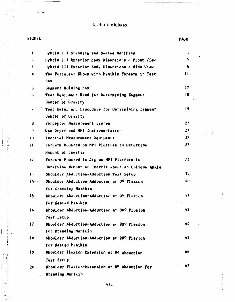
lUT UV VJI( KV
WlUJUId' PAUX
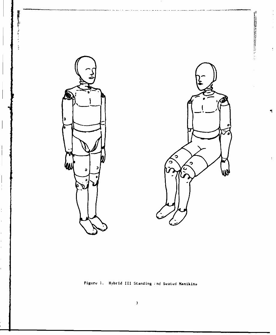
1 Hybrid III Utanding and Uativd Manikins 3
V. Hybrid III Exterior Body Dimensions - front View
3 Hybrid III Exterior Body Dimnsions - Side View 6
4 The Perceptor Shown with Manikin forearm in Test II
BoxU;gment Iflin~, $ox 17
l Toot Equipm nt Ui;od for UDtrLning Stgmont 18
Centvr of Gravity
Tout Uetup and Procvdurt for Dotvtnining Cogment 19
Center of Gtovity
b 'rceptot Measurement byriem 21
1) Gas Dryer and MPI Xnstrume'tatiot, '1
10 Inertlial Heaurement Lquilmert 22
11 Voreru Mourited on MPI Platform to Dewrrou 23
4t(,eirjt of Inertia
12 Yorebru Mountd in Jig on MPI Platform to /1
Dnteruaire Mkent of Inertia about an Oblique Angle
13 :;houldor Abdul-tiorAdduction Tear Setup
14.-- Uhouluvr Abduction-Adducttor at 00 Ilexion 4)
for Lt5.IJit% Manikin
15 Shoulder Abduct ion-Addut ts of U1' VIPxion ',1
for Bested Manikin
16 Shoulder Abductior-Adduction at 900 Floxion 42
Test Setup
17 Obvulder Aduction-Adductiu. at 900 flei.on 44
for Standing Manikin
1b Dhoulder Abduction-Adduction at 900 flexion 4
for Boted Manikin
19 Shoulder Flexion E-ttnsion at 00 Abduction 6
Test Setup
20 Shoulder VIleion-Extenion at 00 Abduction for 67
Standing Manikin
vi I
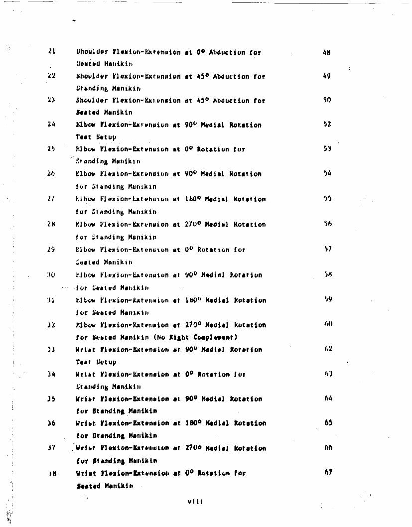
21 Vhouldor ?lyxion-hattnuton at 00 Abduction for 40
Gelated Manikin
22 bhoulder Ylaxion-Exrinnion at 450 Abduction for 49
Oranding Manikin
23 Shouldor Flexion-E1tenaion at 450 Abduction for 50
Seated Manikin
24 Elbow F1exion-Umwpniuion at 900 Medial Rotation 52
Test Setup
2,5 Ybow Vlexion-Extenvton at 00 Rotation for 53
S tandi ng Mariki f,
26 Elbow Vleoxon-.xroniuon at 900 Medial Rotation 54
fur Standing Manikin
)7 F.1bow Vl'xion-JLWtn|atof at Icv at Medial Rotation 5
for Standing Manikin
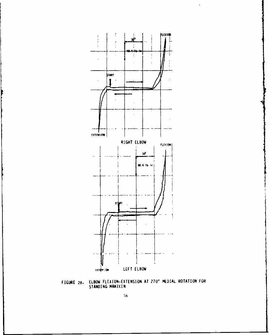
28 Elbow Flexion-Ext4anaion at 27U ° Medial Rotation 50
for Itunading Manikin
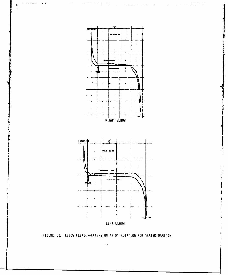
29 Ilbow Vlexion-Extention at 00 Rotation for )7
oatvd Manikin
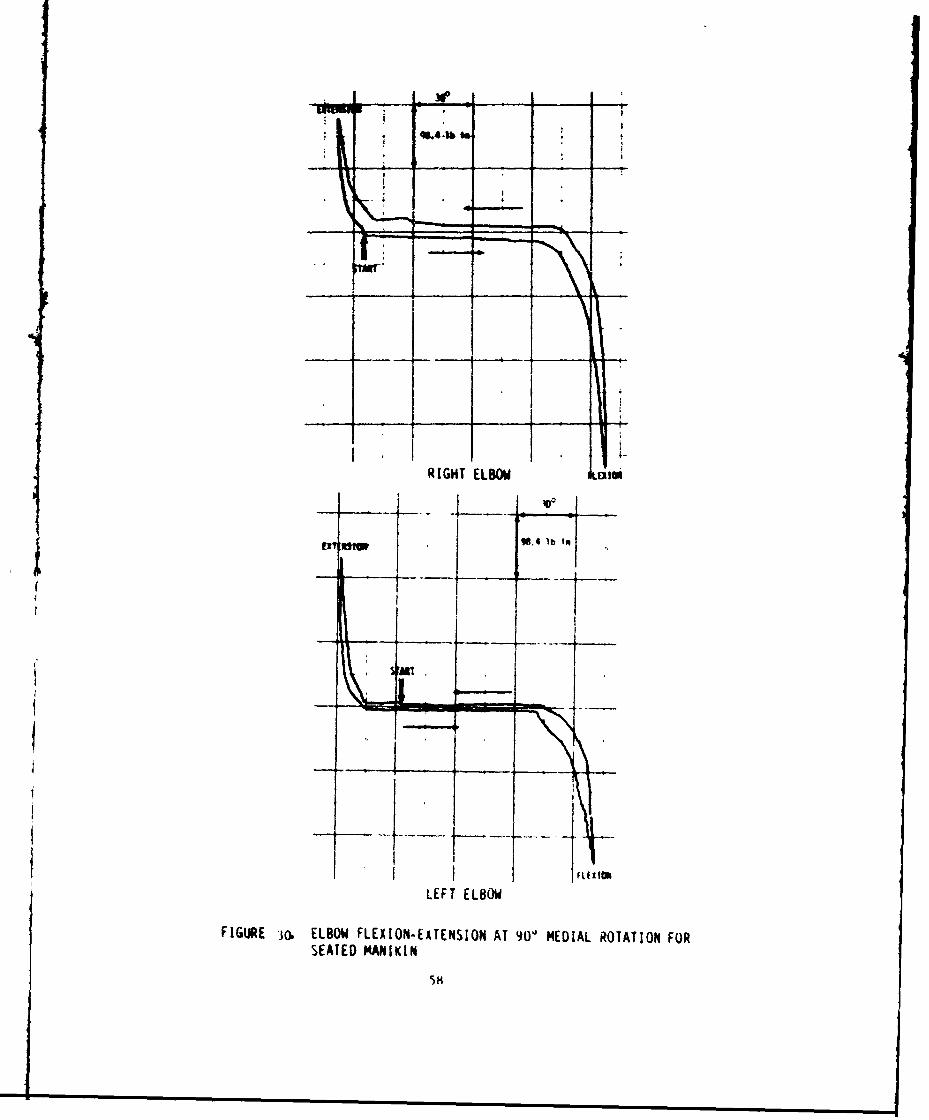
30U 1 lbow Y'l.A,*o-"r t inuon at 900 Medial Potation I8
.. for Ueatvd Manikfii
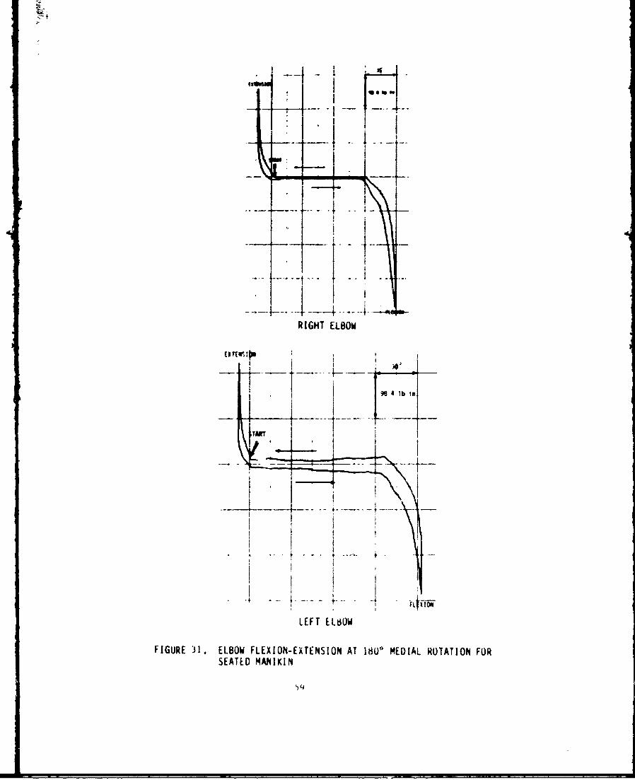
31 FIbow Flexion-xtveliunr at lbo, OMedial Itotation 59
for eatod Maniit|
32 Ylbow Ylexion-K.tersion at 2700 Medial Rotation 60
for Seated Manikin (No Right Ccoplmnt)
33 Wrist Ylexion-IUtvnvion at 900 Madiel Rotation ,2
Teut Detup
34 Wriat Vlexior.-tenaion at 00 Rotation for f3
Standing Manilkit
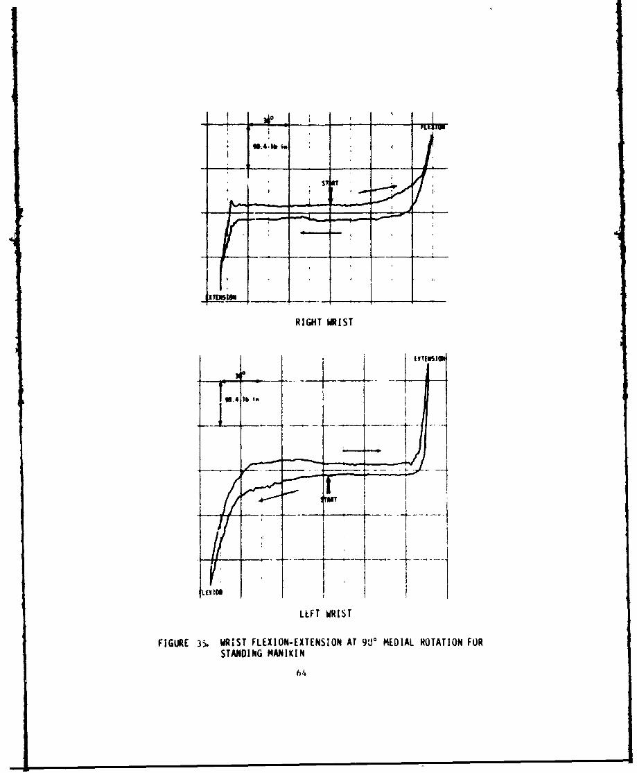
35 Wrist vlexioz-xtonaion at 90° Medial Rotation 64
for Standing Manikin
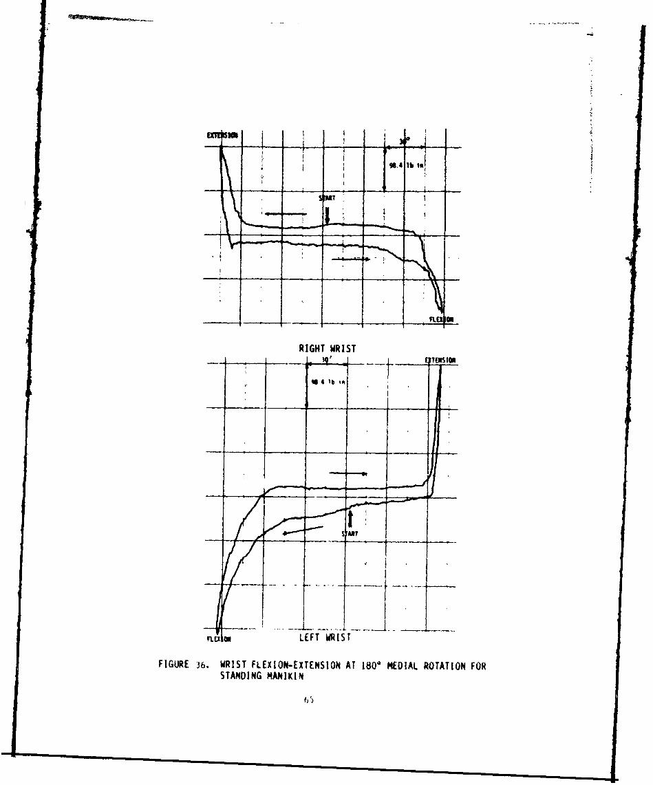
36 Wriat Vlexion-f.xtonuion at 1800 Medial Rotation 65
for Standing Manikin
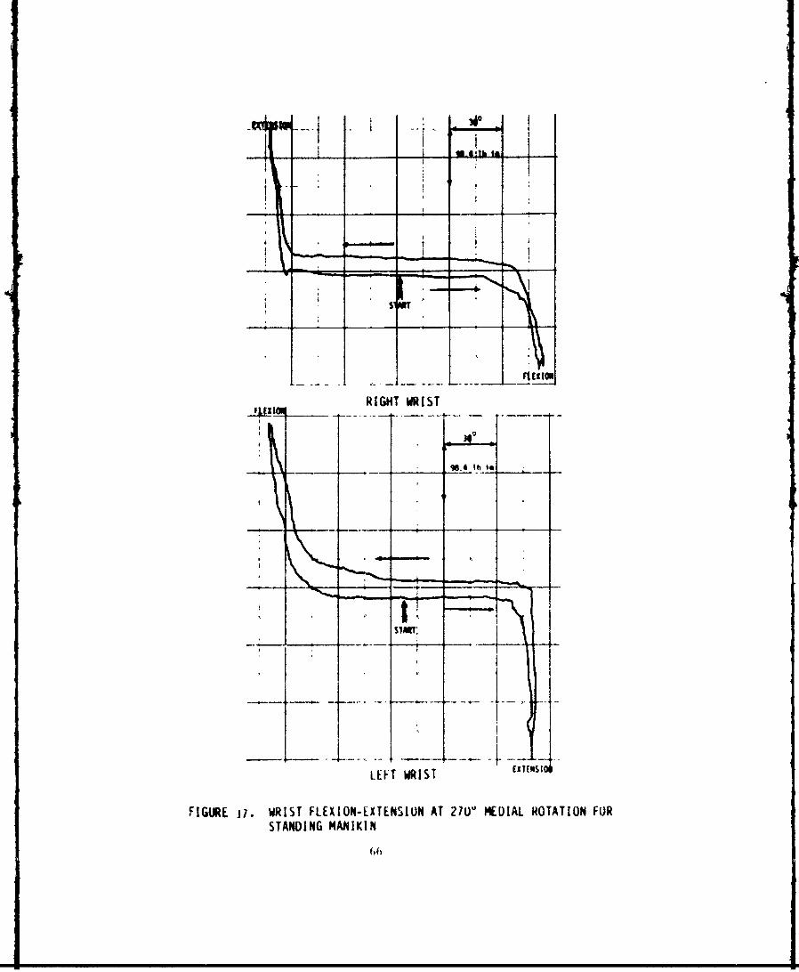
Si - Wrist, Vloxion--KxrUauaton at 2700 Medial Rotation fib
for Standing Manikin
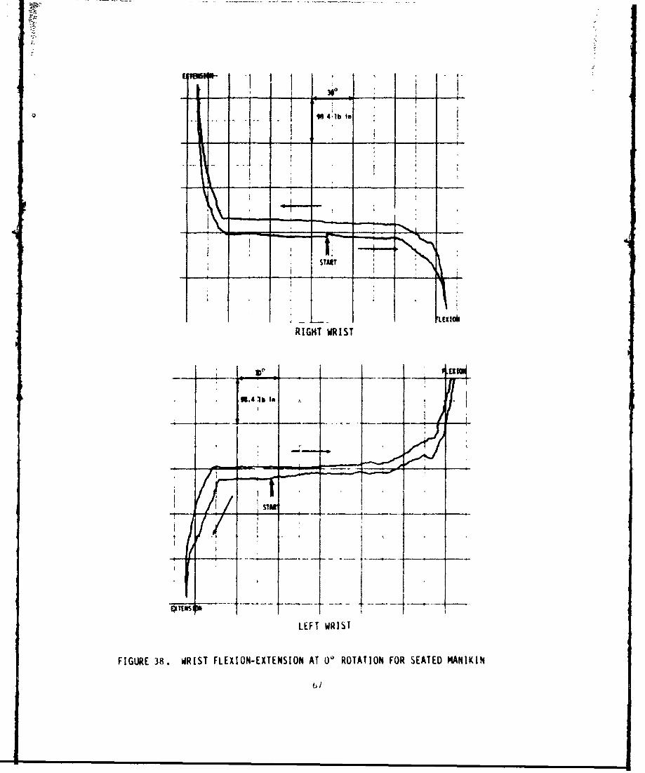
46 Wriat Vlexion-Kxtvnxvu at 00 Rotation for 67
Seated Manikin
viii
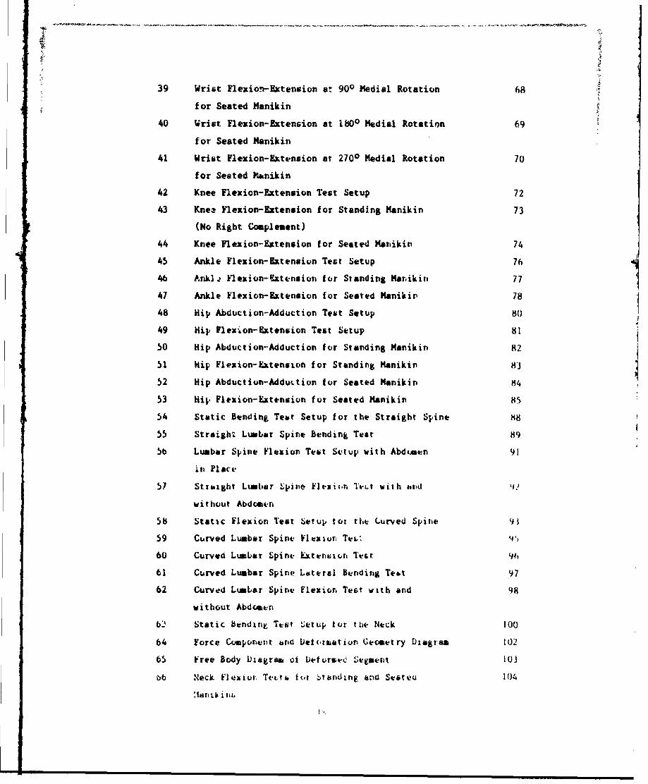
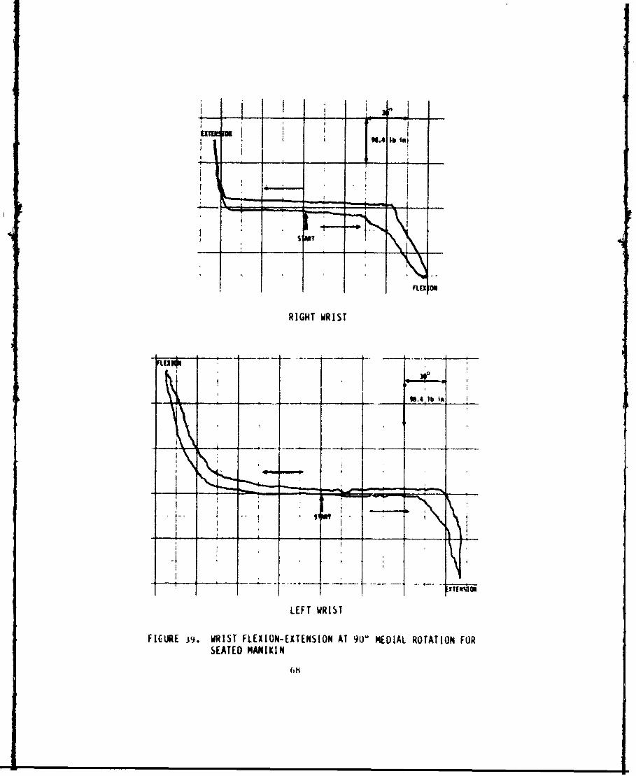
39 Wrist Flexion-Extension at 900 Medial Rotation 68
for Seated Manikin
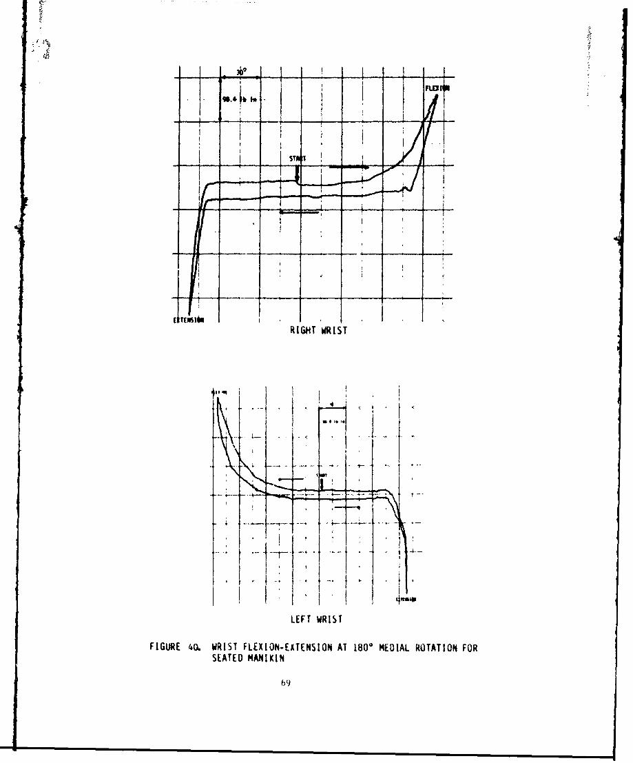
40 Wrist Flexion-Extension at 1800 Medial Rotation 69
for Seated Manikin
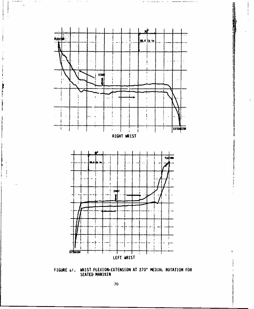
41 Wrist Flexion-Extension at 2700 Medial Rotation 70
for Seated Manikin
42 Knee Flexion-Extension Test Setup 72
43 Knee Flexion-Extension for Standing Manikin 73
(No Right Complement)
44 Knee Flexion-Extension for Seated Manikin 74
45 Ankle Flexion-Extension Test Setup 76
46 Ankla Flexion-Extension for Standing Marikiii 77
47 Ankle Flexion-Extension for Seated Manikin 78
48 Hip Abduction-Adduction Test Setup 80
49 Hip Flexion-Extension Test Setup 81
50 Hip Abduction--Adduction for Standing Manikin 82
51 Hip Flexion-Extension for Standing Manikin 83
52 Hip Abduction-AdduLtion for Seated Manikin 84
53 Hi I. Flexion-Extension for Seated Manikin 85
54 Static Bending Teat Setup for the Straight Spine 88
55 Straight Lumbar Spine bending Test 89
5b Lumbar Spine Flexion Test Setup with Abdomen 91
i.1 Place
57 Stiaight Lumbar "pin~e Fl(-eXi, T*Lt with hild t)?
without Abdomen
58 Static Flexion Test Setup tot the Lurved Spine 91
59 Curved Lumber Spine Flexioro Teit ')
60 Curved Lumbar Spine Extension Test 96
61 Curved Lumbar Spine Lateral Bending Tebt 97
62 Curved Lumbar Spine Flexion Test with and 98
without Abdomen
6- Static Bending Test 1etup for the Neck 100
64 Force Componetit and betuoruation Geometry Diagram 102
65 Free Body Diagram of Defotrae Segment 103
0b Neck Flexiu . Tetts- for tunding acid Seoteu 104
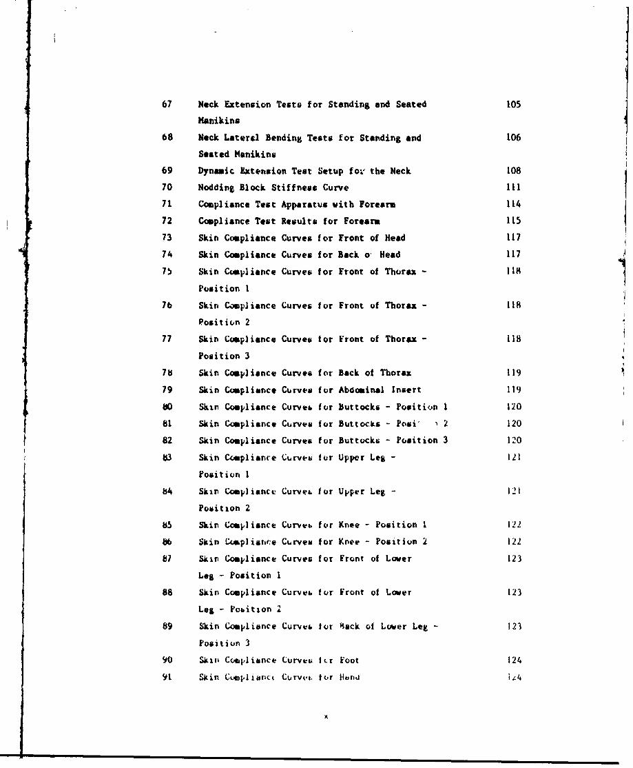
67 Neck Extension Tests for Standing and Seated 105
Manikins
68 Neck Lateral Bending Tests for Standing and 106
Seated Manikins
69 Dynamic Extension Test Setup fov the Neck 108
70 Nodding Block Stiffness Curve 111
71 Compliance Test Apparatus with Forearm 114
72 Compliance Test Results for Forearm 115
73 Skin Compliance Curves for Front of Head 117
74 Skin Compliance Curves for Back o- Head 117
75 Skin Co pliance Curves for Front of Thor" - 118
Position l
76 Skin Compliance Curves for Front of Thorax - 118
Position 2
77 Skin Compliance Curves for Front of Thorax - 118
Position 3
7b Skin Compliance Curves for Back of Thorax 119
79 Skin Compliance Curves for Abdominal Insert 119
80 Sktn Compliance Curves for Buttocks - Position 1 120
bi Skin Compliance Curves for Buttocks - Posi' 2 120
82 Skin Compliance Curves for Buttocks - Position 3 120
3 Skin Compliance Curves for Upper Leg - 121
Position I
84 Skin Compliance Curve. for Upper Leg - 121
Position 2
b5 Skin Compliance Curvet for Knee - Position 1 122
8b Skin CAoplianrte Curves for Knee - Position 2 122
87 Skin Compliance Curves for Front of Lower 123
Leg - Position 1
88 Skin Compliance Curvest for Front of Lower 123
Leg - Pobition A
89 Skin Compliance Curves for Rack of Lower Leg - 123
Position 3
90 Skin' Compliance Curve. fr Foot 124
91 Skin C,elianct Curvet., fr HunJ iz4
> umum um m u um m u umum m u um m u w
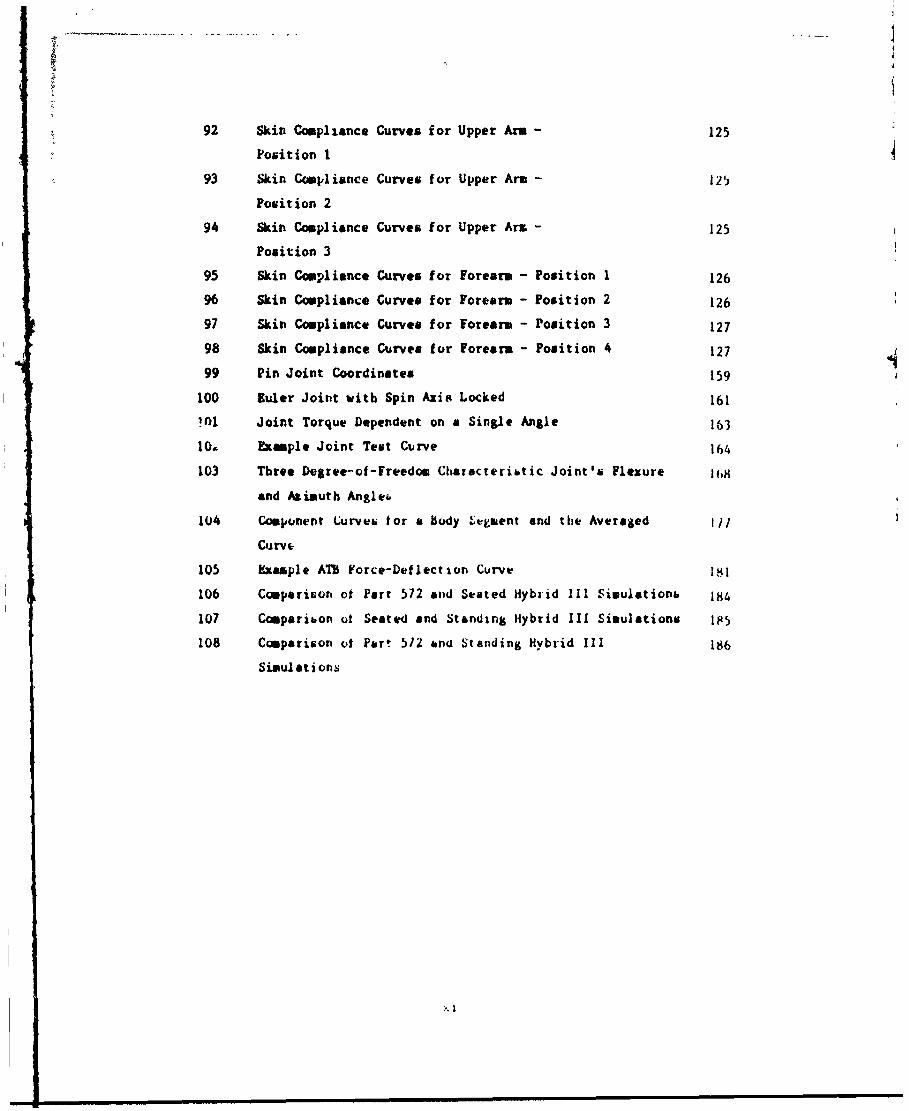
92 Skin Compliance Curves for Upper Arm - 125
Position I
93 Skin Compliance Curves for Upper Arm - I21)
Position 2
94 Skin Compliance Curves for Upper Ar - 125
Position 3
95 Skin Compliance Curves for forearm - Position 1 126
96 Skin Compliance Curves for forearm - Position 2 126
97 Skin Compliance Curves for Forearm - Position 3 127
98 Skin Compliance Curves for Forearm - Position 4 127
99 Pin Joint Coordinates 159
100 Ruler Joint with Spin Axis Locked 161!11 Joint Torque Dependent on a Single Angle 163
0a. Emple Joint Test Curve 164
103 Three Degree-of-Freedom Characteriitic Joint's Flexure 11,8
and Azimuth Angle&
104 Component Curveh tor a Body ' egment and the Averaged I/1
Curve
105 Mxasple ATB Force-Deflection Curve 181
106 Comparison ot Part 572 and Seated Hybrid III Simulationm 184
107 Comparibon ot Seated and Standing Hybrid III Simulations I5
108 Comparison ot Par! 5/2 and Standing Hybrid III 186
Siamulations
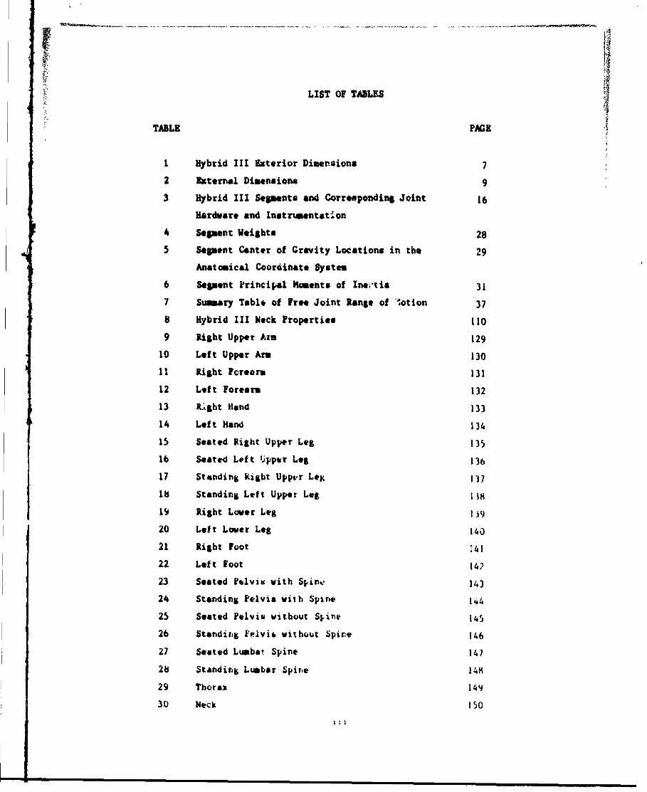
LIST OF TABLES
TABLE PAGE
1 Hybrid III Exterior Dimersiona 7
2 External Dimensions 9
3 Hybrid III Segments and Corresponding Joint 16
Hardware and Instrumentation
4 sent Weights 28
5 Segment Center of Gravity Locations in the 29
Anatomical Coordinate System
6 Sepent Principal Moments of Ins-tia 31
7 Summary Table of Free Joint Range of "otion 37
8 Hybrid III Neck Properties 110
9 Right Upper Am 129
10 Left Upper Arm 130
11 Right Fcreerm 131
12 Left Forearm 132
13 R:%ght Hand 133
14 Left Hand 134
15 Seated Right Upper Leg 135
16 Seated Left 'Upptr Leg 136
17 Standing kight Upper Leg 137
18 Standing Left Upper Leg i)8
19 Right Lover Leg IJ9
20 Left Lower Leg 140
21 Right Foot :41
22 Left Foot 14?
23 Seated Pelvid with Spinre 143
24 Standing Pelvis with Spine 144
25 Seated Pelvis without Spine 145
26 Standing Pelvi& without Spire 146
27 Seated Lumba! Spine 147
2b Standing Lumbar Spine 148
29 Thorsa 149
30 Neck 150
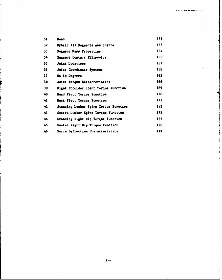
31 Head 151
32 Hybrid III Segento and Joints 153
33 Segment Mass Properties 154
34 Seement Contact Ellipsoids 155
35 Joint Locations 157
36 Joint Coordinate Systems 158
37 OD in Degrees 162
38 Joint Torque Characteristics 166
39 Right Sboulder Joint Torque Function 169
40 Head Pivot Torque Function 170
41 Neck Pivot Torque Function 171
42 Standing Lumbar Spine Torque function 172
43 Seated Lumbar Spine Torque Function 173
44 Standing Right Hip Torque function 175
45 Seated Right Hip Torque Faction 176
46 Force beflection Characteristics 179
Ixv
*I
1.0 INTRODUCTION
The use of ansiyticol computer based models for the prediction of human
response to mechanical forces for both safety evaluation of various
systems and the design of new systems is becoming a standard practice.
This is particularly true in the area of automobile crash and subsequent
occupant reponse investigations and in studies of crewmember responses
during ejection from aircraft. In these applications. as weil as
others, the use of models is a complementary process to physical system
tooting and provides considerable benefits in an overall program seeking
to identify and quantify potential systm hazards and subsequently
provide direction for system improvement. Specifically, modals can be
beneficial in reducing the number of required tests and thus reducing
program cost; they provide insigbt into various physical mechanisms that
may be occurring but whicb may not be obvious or readily observed in
actual testing; they allow fcr a convenient means of investigating the
effects of parameter changes; they can be used in test design to define
the optimum corfiguration and conditions; they can be u&ed independently
of an actual test to investigate the general feasibility of concepts;
and ultimately, with sufficient validation and a soundly developed data
base, they may be used directly as an injury assessment tool. While
these benefits are substantial their realization requires not only a
sounr analytic methodology but also an appropriate and soud oats base
that properly characterizes the system being modeled.
This program has sought to develop such a data base for the Hybrid III
dummy. The Hybrid III dummy is extensively used in automotive crash
testing, is generally considered to be the most advanced of automotive
testing dummies currently available and is in the process of being
adopted by the National Highwaiy Traffic Safety Administration as astandard for automotive safety compliance testing. While the ultimate
objective of this program was to develop a data base for the Crash
Victim Sisulator (CVS) ad Articulated Total Body (ATB) computer models
by reducing the data to the exact input formats required for these
prograRs, the directly measured data is also presented to provide an
explanation of the methodology used iv measuring the dummy properties
and also to provide data that users of other models could reduce
according to their model input formatting requirements.
The measurement objectivex in this program, though not necessarily the
methods, are the saw as in the study on the Part 572 dumm7 conducted by
Flec, at al [ll. The Part 572 dumay is a derivative of the General
Motors Hybrid Il dummy which. in many respects, is similar to the
presently investigated Hybrid Ill dummy. While a direct comparison of
the data sets is not made in this report. simulations with identical
dynamic. exposure conditions were performed using the Port 572 and Hybrid
III dummy data sets and the results are reported.
Two Hybrid III dtmie were measured in this stuc.#. An illustration of
the two types of manikins, standing and stated, is shown in Figure 1.
One dummy had freely articulating hips, is comnly referred to as &
pedestrian testing dummy. and in this study is denoted as the standing
dummy. The other dummy was the standard Hybrid III with a pelvis
section molded in a sitting position. This dumy is denoted as the
seated dummy. The intent of this program was tc develop one standard
data set for the Hybrid III and in effect. this was done with the seated
dummy date base. However. the pelvic and upper leg structure of the
standing dummy was substantially different atod thus a different data set
was developed for this portion of the body. The result was that all
body data properties for the two dummies and their left and right sides
were averaged to produce one common date set for the total body, except
for the pelvis (including lumbar spine) and uppet legs. Two data sets
were prepared for the pelvis and upper legs and each combined with the
common, averaged data set to form the seated and standing Hybrid Ill
data seto.
This report describes the measurement methodology, the results of the
measurements,. the data reduction methods, the assumptions and methods
for reformatting to the CVS/ATS model format and a demonstration
simulation cooparing the Part 572 and Hybrid III duamy responses under
identical conditions.
2
1.
I-
- i -
9, !00
Figurv I. Hybrid III Standing ;nd Seated Manikinb
3
2.0 TEQINICAL DISOJSSION
2.1 Physical Measurement of Mpn:ikin Properties
In this section the various physical measurements that were made on
both sanikit.s are presented and discussed. In general, each
subsection presents and discusses the procedure developed, the
equipment used and includes both a presentation &nd discussion of the
results obtained. Each pertinent data set. i.e. mass properties.
external dimensions, joint characteristics. etc, has been separated
into the various subsections for clarity and for easy reference.
2.1.1 Measurement of Manikin External Dimensions
2.1.1.1 Description of Measurement Procedure
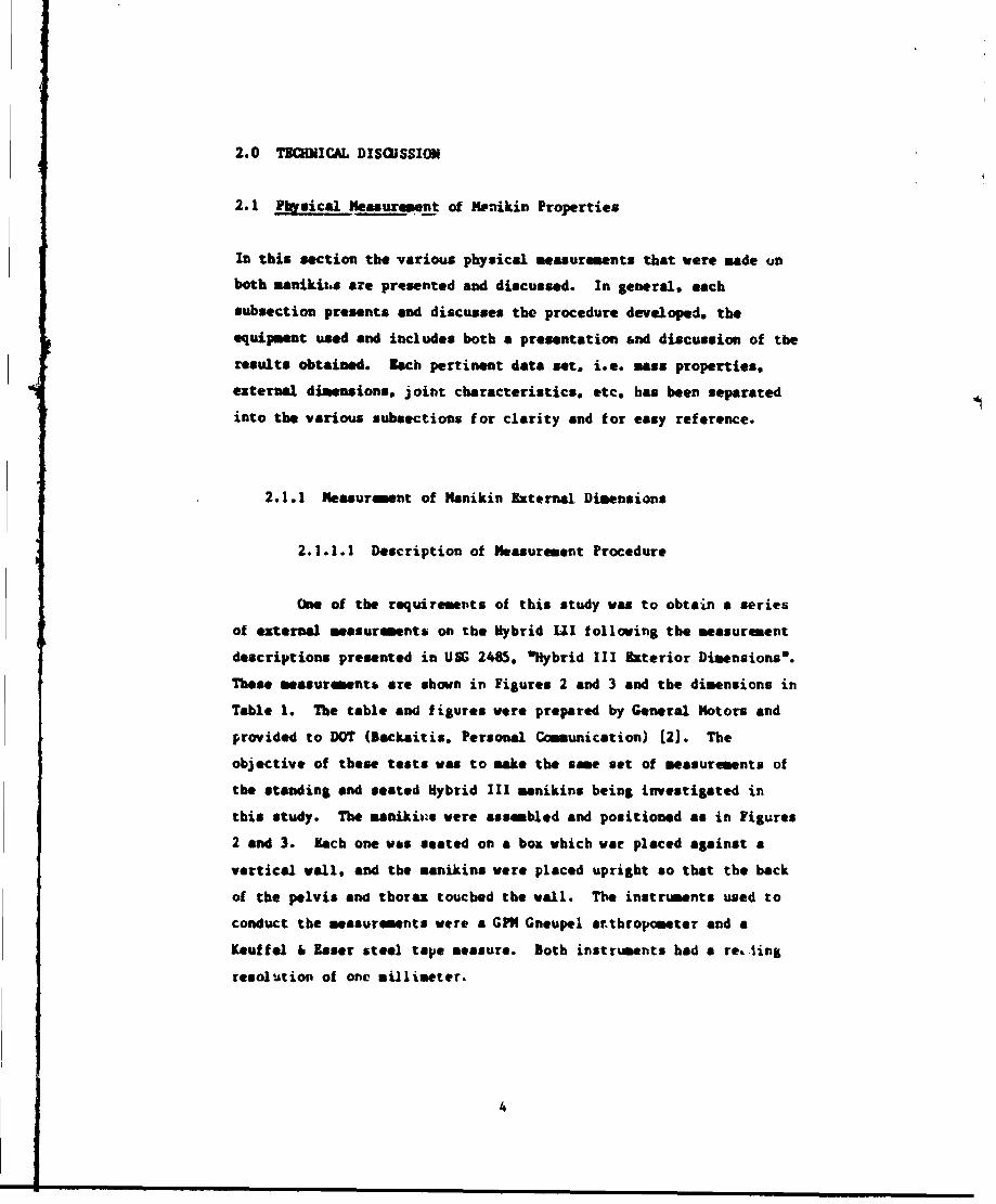
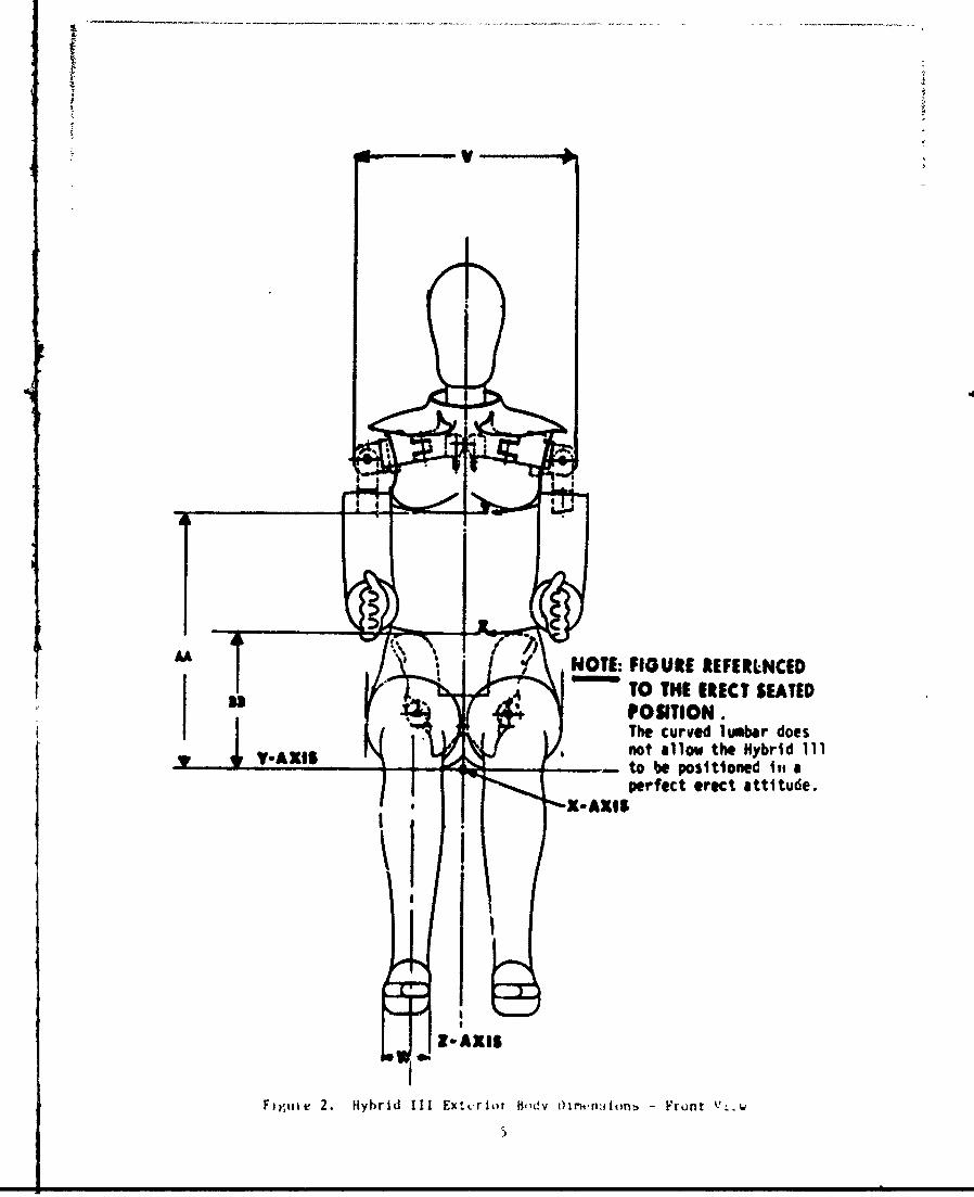
One of the requirements of this study was to obtain a series
of external measurements on the Hybrid UI following the measurement
descriptions presented in USG 2485. "Hybrid III Exterior Dimensions*.
These msurwntab are shown in Figures 2 and 3 and the dimensions in
Table 1. The table and figures were prepared by General Motors and
provided to DOT (Backaitis. Personal Communication) [2). The
objective of these tests was to make the sone set of measurements of
the standing and seated Hybrid III manikins being investigated in
this study. The manikiis were assembled and positioned as in Figures
2 and 3. Each one was seated on a box which vat placed against a
vertical wall, and the manikins were placed upright so that the back
of the pelvis and thorax touched the wall. The instruments used to
conduct the measurements were a GPM Gneupel arthropcmeter and a
Kuffel & Easer steel tape measure. Both instruments bad a re. Aing
resolution of one millimeter.
4
AA NOTE: FIGURE REFERLNCEDTO THE ERECT SEATEDPOSITION.The curved lumbar does
T-AXISnot allow the Hybrid 111to be positioned iii a
X-XSperfect erect attitude.
FigLet 2. Hybrid III Extvrior Bt~v 0iion:t,~ - Fro~nt V ..w
- ~ ~ I Ih REC IFAMIPO~flO .The curved lubar does not allowthe Hybrid Ill to be positionedin a perfect erect attitude.
Figuxe~ 3. Hybrid .!I Exterior Body Diaenoions Side View
6
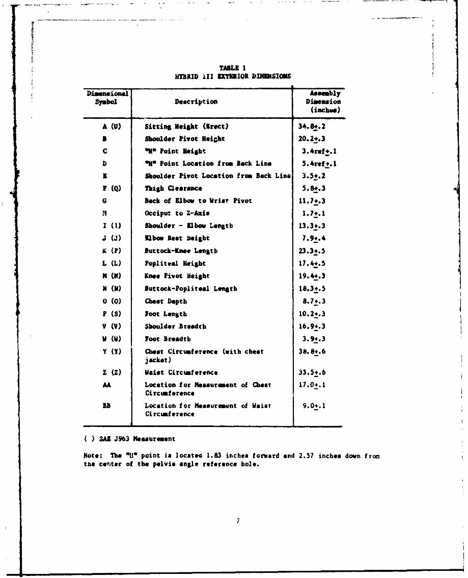
TABLK 1HYBRID Il ECTIOR DIHg4SIONS
Dimensional AsmblySymbol Description Dimension
Cinches)
A (U) Sitting Height (Erect) 34.8_.2
a Shoulder Pivot HeiGht 20.2+.3
C *' Point eight 3.4ref+.1
D " Point Location from Back Line 5.4ref+.l
9 Shoulder Pivot Location from Back Line 3.5±.2
F (Q) Thigh Clearance 5.8+.3
G back of Elbow to Wrist Pivot 11.7,.3
Occiput to Z-Axis 1.7.1
I (1) Bboulder - Kibow Lengtb 13.3+.3
J (J) Elbow Reat Height 7.9.4
It (P) Buttock-knee Length 23.3+.5
L (L) Popliteal Height 17.4+.5
M (H) Knee Pivot Height 19.4.3
N (N) Buttock-Popliteal Length 18.3+.5
0 (0) Chest Depth 8.7+.3
P (S) loot Length 10.2+.3
V (V) Shoulder Breadth 16.9+.3
W () loot Breadth 3.9+.3
y (y) Chest Circumference (with chest 38.8+.6jacket)
Z (Z) Waist Circumference 33. 5.6
AA Location for Measurement of Chest 17.0+.1Circumference
RD Location for Measurement of Waist 9.0+.1Ci rcomference
( ) SAE J963 Neasurement
Note: The "iO point is locateo 1.83 inches forward and 2.57 inches down fromthe ceriter of the pelvis angle reference bole.
I,
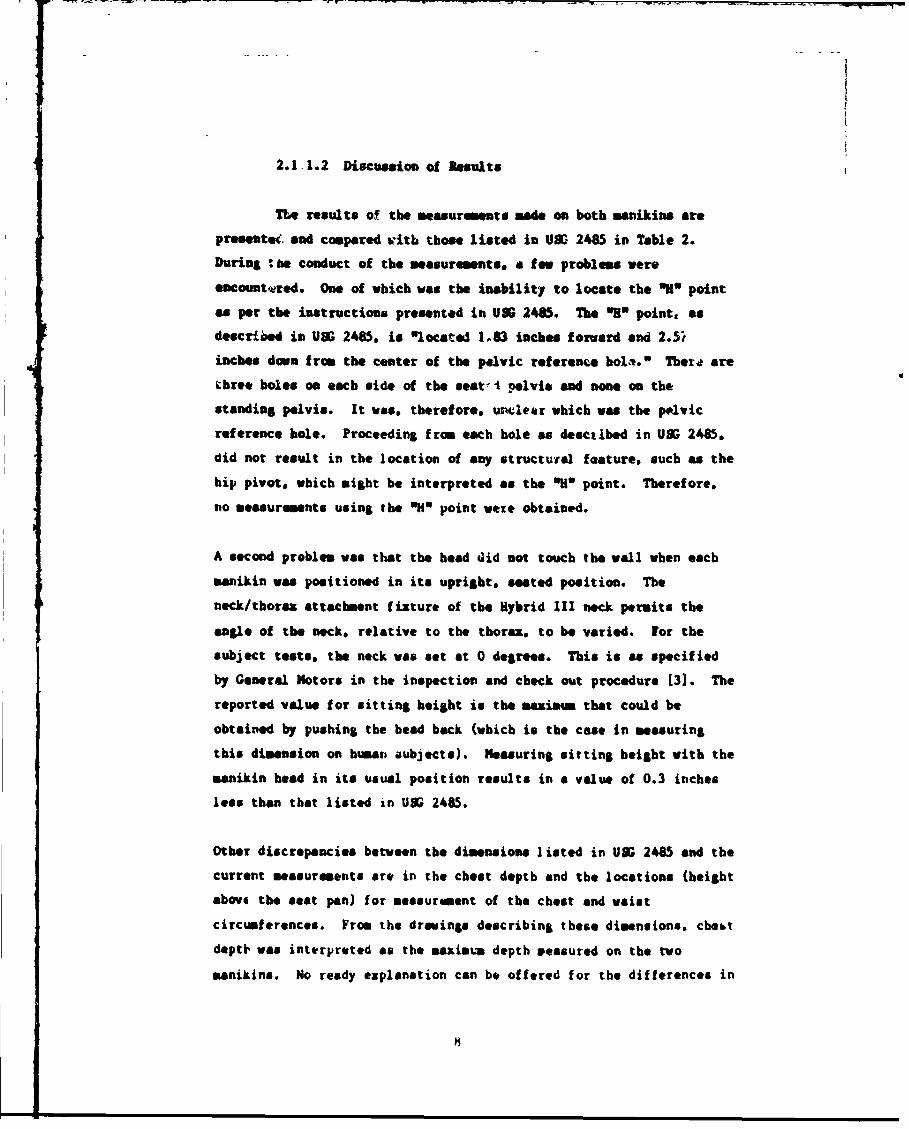
2.4. Discussio, of Results
The results of the measure-meto made on both manikins are
pre"Ste. and compared with those listed in USD 2485 in Table 2.During *#bie conduct of the measuremets. a few problems were
eflountvred. One of which was the inability to locate the OR*' pointas per the instructions presented in U39 2465. The "B" point, as
described in UBG 2465. is "located 183 inches forward and 2.5iinches doiwn from the center of the pelvic reference bolmher W4 aretbre* holes on each side, of the seat i pelvi, and none on thestanding pelvis. It was, therefore unctlear which was the pelvicreference hole. Proceeding from each hole as deactihe4 in UB 2485.
did not result in the location of any structural fature. such as thehip pivot. which might be interpreted as the "11O point. Therefore.
no measurements using the "NO point wet* obtained.
A second problem was that the head d~id not touch the wall when each
manikin was positioned in its upright. seated position. Theneck/thoraz attachment fixture of the Hybrid III neck permits the
angle of the neck, relative to the thorax. to he varied. For thesubject tests, the neck was set at 0 degrees. This is as specifiedby General Motors in the inspection and check out procedure [31. The
reported value for sitting height is the maximum that could heobtained by pushing the bead back (which is the case in measuringthis dimension on humaga aubjects). Measuring sitting height with the
manikin head in its usual position results in a value of 0.3 inches
less than that listed in USG 2485.
Other discrepancies between the dimensions listed in US; 2485 and the
current measurements are in the chest depth and the locations (height
abowt the seat pan) for measurement of the chest and waist
circumferences. From the drawings describing those dimensions. che~t
depth was interpreted as the maximum depth veasured on the two
manikins. No ready explanation can be offered for the differences in
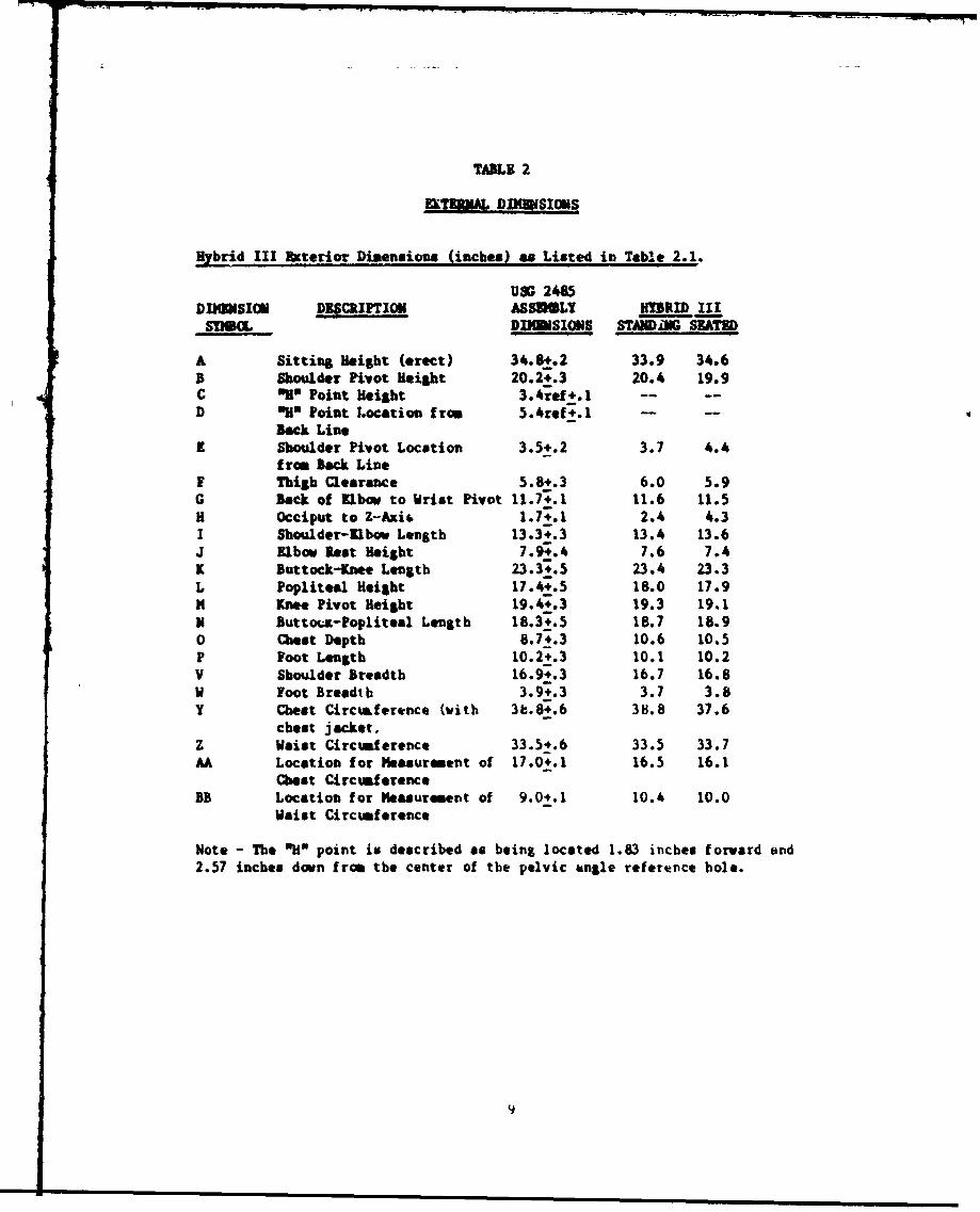
TABLE 2
&ENA DIUSICUS
Hybrid III ftterior Di ensions (inches) as Listed in Table 2.1.
USG 2485DIDSION DESCRIPTION ASSEMLY HY5RID IIISOMa., DIMuSIOMS STADMG STE)
A Sitting Height (erect) 34.8+.2 33.9 34.6B Shoulder Pivot Height 20.2+.3 20.4 19.9C "So Point Height 3.ref +.1 -- --
D "HO Point Location from 5.4ref_.l - -
Beck LineR Shoulder Pivot Location 3.5+.2 3.7 4.4
from Beck LineI Thigh Clearance 5.8+.3 6.0 5.9G Back of Elbow to Wrist Pivot 11.7+.1 11.6 11.5H Occiput to Z-Axi& 1.7+.l 2.4 4.3I Shoulder-lbow, Length 13.3+.3 13.4 13.6J Elbow Rest Height 7.9+.4 7.6 7.4K Buttock-Knee Length 23.3+.5 23.4 23.3L Popliteal Height 17.4.5 18.0 17.9H Knee Pivot Height 19.4_.3 19.3 19.1V Buttova-Popliteal Length 18.3+.5 18.7 18.90 Chest Depth 8.7+.3 10.6 10.5P Foot Length 10.2+.3 10.1 10.2V Shoulder Breadth 16.9+.3 16.7 16.8W Foot Breadth 3.9+.3 3.7 3.8Y Chest CircuLference (with 3b.8+.6 38.8 37.6
chest jacket,Z Waist Circtmference 33.54.6 33.5 33.7A Location for Measurement of 17.0+.I 16.5 16.1
Chest CircumferenceB3 Location for Measurement of 9.0+.1 10.4 10.0
Waist Circumference
Note - The Oi point is described as being located 1.83 inches forward and2.57 inches down from the center of the pelvic angle reference bole.
m i u n m i m u n N p me m iuuno n9
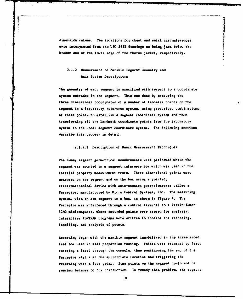
dimension values. The locations for chest and waist circumferences
were internreted from the USG 2485 drawings as being just below the
breast and at the lower edge of the thorax jacket, respectively.
2.1.2 Measurement of Manikin Segment Geometry and
Axis System Descriptions
The geometry of each segment is specified with respect to a coordinate
system embedded in the segment. This was done by measuring the
three-dimensional coordinates of a number of landmark points on the
segment in a laboratory reference system, using prescribed combinations
of these points to establish a segment coordinate system and then
transforming all the landmark coordinate points from the laboratory
system to the local segment coordinate system. The following sections
describe this process in detail.
2.1.2.1 Description of Basic Measurement Techniques
The dummy segment geometrical measurements were performed while the
segment was mounted in a segment reference box which was used in the
inertial property measurement tests. Three dimensional points were
essured on the segment and on the box using a jointed.
electromechanical device with axis-mounted potentiometers called a
Perceptor. manufactured by Micro Control Systems. Inc. The measuring
system, with an arm segment in a box. is shown in Figure 4. The
Perceptor was interfaced through a control terminal to a Perkin-Kmer
3240 minicomputer, where recorded points were stored for analysis.
Interactive VORTRAN programs were written to control the recording.
labelling, and analysis of points.
Recording began with the manikin segment immobilized in the three-sided
test box used in mass properties testing. Points were recorded by first
tntering a label through the console, then positioning the end of the
Perceptor stylus at the appiopriste location and triggering tht
recording with a foot pedal. Some points on the segment could not be
reached because of box obstruction. To remedy this problem. the segment
I0
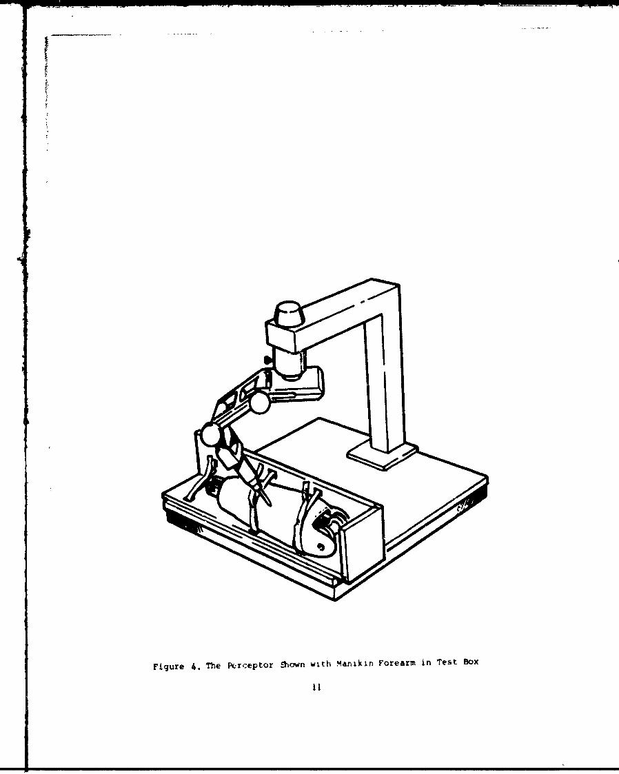
Figure 4. The Ptrceptor -Sown with Manikin Forearm in Test Box
vaa. removed from the box after recording at least three non-colinear
reference points on both the box and segment, then repeating the
recording of -.eppent raeterence point- along with the: other desired
points. This procedure permitted the calculation of transformation
matrices which defined the three-dimensional displacements of the
4ifferent sets of points into a common axis system.
2.1.2.2 Definition and Location of Landmarks and Axis Systems
In order to compare the data measured for the Hybrid III with three
dimensional human data. a series of landmarks were recorded which were
analogous to the anthropometric landmarks used to define the axes on
stereophotogrametrically recorded data of adult men and women [4J &
[5]. Points for defining joint and joint axes locations were also
recorded and were ustd as the basib for defining local mechaniLal
coordinate systems which were directly related to the mechanical
structure of the manikin. The criteria for locating "anatomical"
landmarks on the manikin were their spatial relationship with relevait
structural features (i.e.. joirts), the similarity of the manikin
external geoametry to humans. and the desirability of having axes defined
by landmarks on the sepent ivself. This procedure was hindered b)
structural and geometric features which were dissimilar to humans ur tot
present, and by the fact that a lenduark may not. even in humans. be
located on the relevant segment. For exam[l*. the upper arm anatcAical
axes are defined by three anatoMiLal landmarks which would not be
considered to be present on the Hybrid III upper arm (see Table 9. Right
Upper Arm). Acromiale. the lateral-most point on the acromion process
of the shoulder (part of the Hybrid IIl torso), was located for the
upper arm ei the superior edge of the lateral side of the soft covring.
The lateral and medial humeral epicoind)le in humans are located ot, the
Lpper arm, but also define the elbow axiv. In the Hybrid III, the
surface covering the elbow ia pait of the forearm (Lew Table 11. Right
forearm). Thus. for the purpose of definirg the upper arm axes. the
epicondyles on the upper are were located at the medial and lateral
inferior edges of the uoft covering. While none of the three
axis-defining landmarks for this segment are in thr ideal locations, the
12
plans are analogous to the huan system and permit a reasonable
comparison between human and manikin properties.
Lc Section 2.1.6 presents the definitions of each of the landmarks used to
define axes for each of the Hybrid III axis systems. Most lundmarks
were located at positions that were reasonable analogues of those of
humans, or. as in the upper arm, in positions which would define
anatomical axes as similar as possible to those defined for humans in
the stereophotometric studies.
The anatomical axes are Senerslly defined by two vectors, i end b.
formed by three non-linear landmarks on the segment surface. The
vectors a and V define a plane, with ' X b c defining a vector normal
to the plane which is orthoganal to both ' and b. The directions o. a
and ' are chosen so that the directions of the axes follow the general
convention of z forward, y to the left, and a upward. In order to
assure the proper orientation of these axes and the desired location of
the origin, sometimes more than three points are used to specify tb
axis vectors and origin. The individual axis systems are defined.
segment by segment, in section 2.1.6.
2.1.2.3 Transformation of Data Between Axis Systems
Three-dimensional coordinates of points are initially measured on the
sepents and the box by the Perceptor and recorded in a laboratory
reference system designated by L Three points on the box are used to
define a coordinate system designated by B. and all the points are
transfornea to this box coordinate system. This system is used in the
measurement and calculation process of segment inertial properties.
From the points measured on the segment& and the inertial property
measurements, thret *,gmeht base coordinate systems are calculated. Ai
anatomical system designated by A and defined by equivalent anatomical
surface landmarks; a local mechanical reference system designated by L
and defined by segment mechanical features, for example joint cent. rs
and rotation axes; and a principal axeb vyste" designated by P and
13I

obtained by segment inertia tensor diagonalization are established and
transfomations between thew calculated.
These transformations are in the form of 3X3 cosine matrices, and their
operation on vectors is siven by
rL = AArA
vhere rA, rL, rp are the same vectors but with components in the
anatomical, local and principal coordinate systems respectively.
The cosine matricea. [AJ. are orthogonal and have the corvenient
property it two are know the third can be calculated by the matrix
product
A AIAAMK.
It was decided to pres.nt the results of the testing of the two Hybrid
III manikins in the fors of a mean reFresentative data set. As
described below, the method for a:riving at the representative geometry
is in part an averaging of the two manikins, and in part an effort to
account for the uysmatry designed into the manikins. Each of the limb
uegents. four data sets, right and left from both manikins. woere
combined (exceptions wcre the upper leg. pQlvis. a:.-' spine which
differed in the manikins and were treated separately). For the axial
segments - head, neck, thorax, and pelvis - airrozed data sets were
created so that a symmetrical representation vould result.
The component of the vector from, the local rrference origin (center of
mass) to a joint center was reflected from the right side to( the left
gide by changing the vigns. The mirror images of axial segmentu (head.
neck, thorax. and pelvis) wete created by averaging the values of right
and left side landmarki.
I I,
The mean value of the Wv vector was calculated for each body segment.
This vector was noted to have a random lateral variation about the
segment long axis. so an adjustment for consistency was node by setting
the Y coordinate value to 0.0.
The results are presented for each segment in section 2.1.6 where the
representative values of the landmark coordinates in local reference and
anatomical axes are presented along with the matrix (AAL) for
transforming points from local to anatomical systems.
2.1.3 Measurement and Determination of the Mass Properties of
'b.e Manikin Segments
2.1.3.1 Discussion of Measurement Techniques and Equipment
Utilized
2.1.3.1.1 Segment Mass
The equipamnt used to measure the mass of the manikin segments vab an
electronic weighing scale and a segment holder, a three sided
rectanpular balsa wood box. The mass properties of t e balsa boxes were
seasted beforehand and storri in data files on a supporting Hewlhtt
Packard 85-B microcomputer. The segment was extracted from adjoiriing
segments and tested with the joint hardware as listed in Table 3. The
segmnt was weighed ir, the box and the box weight was subtracted to
obtain the segment weight. These boxes provided a means to easily and
securely house the manikin segment in & fixed position while its masr
properties were being detemined. A representative box is shown in
Figure 5. A velcro strap was used. alonig with masking tape when
necessary, to rigidly fasten the sebment within the box so that no
relative notion was possible.
II'
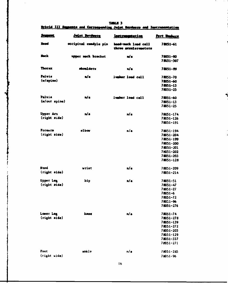
TAOLm 3
Need eccipite ceamdyle pin hued-meek 1o1d cell 76051-61three Secelerunmters
Neck uper mek bracket 0/0 76051-907M051-307
Tboraz shoulders a 78051-89
Pelvis a/0 lIuber load cell 76051-70(v/Spim ) 78051-60
78051-1378051-25
Pelvis 0/0 lumber lod cell 78051-60(v/our spine) 78051-13
78051-25
Upper Aim a/s n/a 78051-174(right side) 78051-126
78051-191
Forearm elbow u/4 78051-194(right side) 78051-204
78051-19978051-20078051-20178051-20270051-20378051-128
K1nd wrist A/a 78051-209(right side) 76051-214
Upper Let hip n/S 76051-51(right side) 78051-47
78051-2778051-678051-72780S1-9678051-276
Lower Log knee n/s 78051-74(right side) 78051-278
78051-13978051-27278051-20378051-12978051-3377051-271
Foot ankle n/s 18051-285
(right bide) 71051-96
16
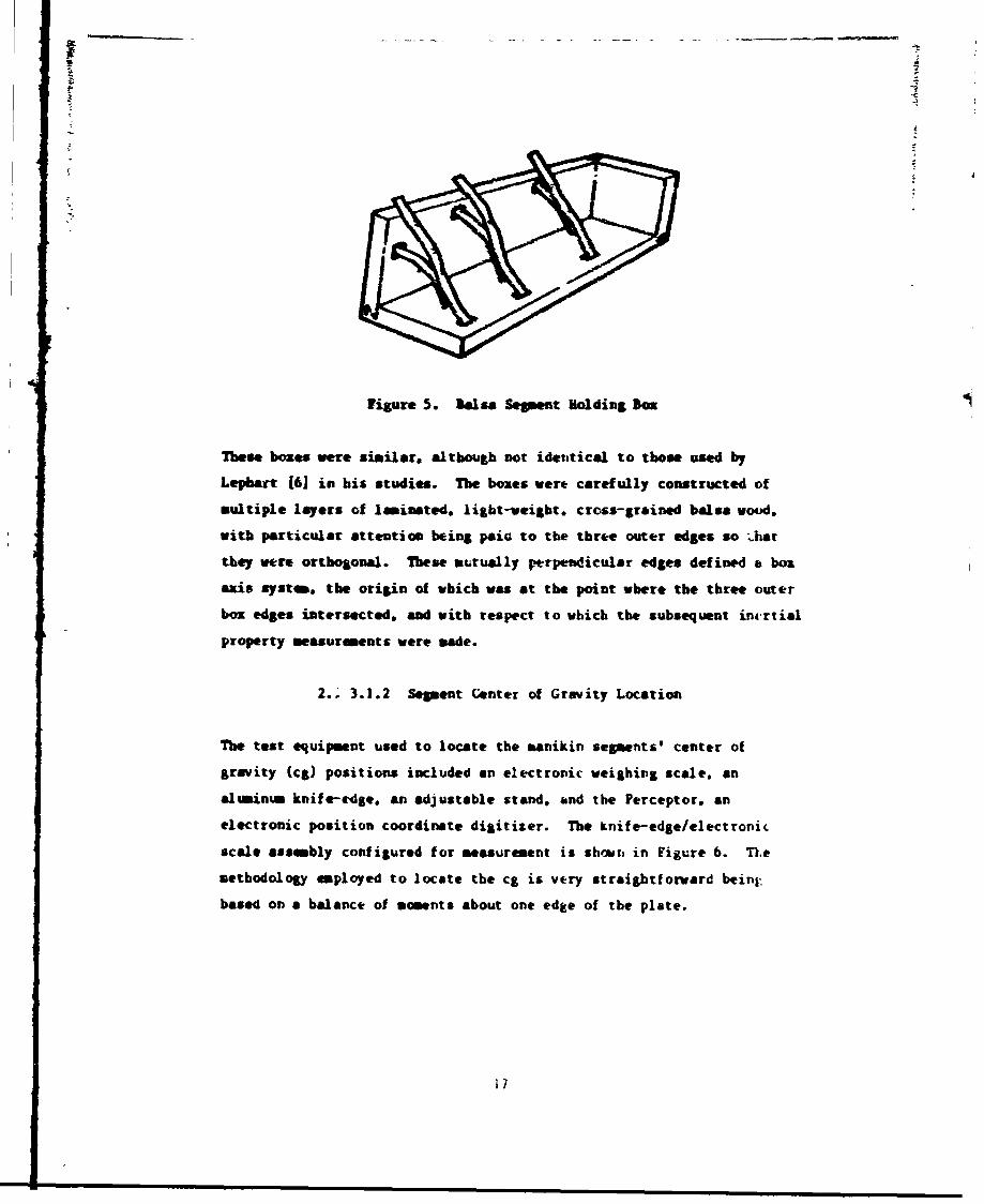
figure 5. Uals Segment Holding lox
These boxes were similar. although not identical to those used by
Lepbart 16i in his studies. The boxes were carefully constructed of
multiple layers of laminated, light-weigbt. cross-grained balsa wood.
witb particular attention being paia to the three outer edges so .hat
they were orthogonal. These mutually ptrpendicular edges defined a box
axis system, the origin of which was at the point where the three outer
box edges intersected, and with respect to which the subsequent incrtial
property measurements were made.
2.. 3.1.2 Segment Center of Gravity Location
The test equipment used to locate the manikin segments' center of
gravity (Ug) positions included an electronic weighing scale, an
alumintm knife-edie, an adjustable stand, and the Perceptor. an
electronic position coordinate digitizer. The knife-edge/electronic
scale assembly configured for measurement is sbowi, in Figure 6. TIe
methodology employed to locate the cg is very straightforward beini-
based on a balance of moments about one edge of the plate.
17
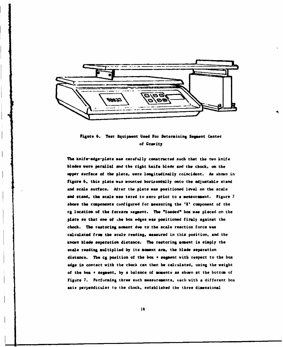
figure 6. Tesr 8quipsent Used For Determining Segment Center
of Gravity
The knife-edge--plate, was carefuslly construhcted such that the two knife
blades were parallel and the right knife blade and the chock, on the
upper surface of the plate. were longitudinally coincident. As shown in
Figure 6. this plate was mounted horisoelly onto the adjustable stand
and scale surface. After the plate wasn positioned level on the scale
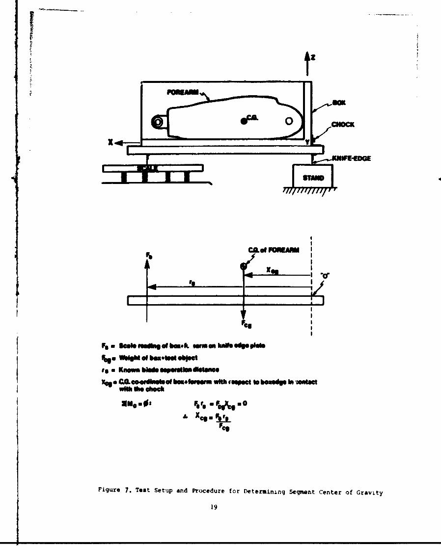
and stand, the scale was tared to sero prior to a meaurmnt. Figure 7
sbows the components configured for measuring the W1 coponent of the
cS location of the forearm segment. The *loaded' box wao placed on the
plate so that One Of hbe box edges was positioned firmly against the
chock. The restoring moment due to the scale reaction force was
calculated fro tbe scale reading. measured in this position, and the
known blade separation distance. The restoring moment is simply the
scale reading multiplied by its moment arm, the blade separation
distance. The cg position of the box + segment with respect to the box
edge in contact with the chock can thee. be calculated, using the weight
of the box + segment, by a balance of moments as shown at the bottom of
Figure 7. Performing three such measurements. each with a different box
axis perpendicular to the chock, established the thre* dimensional
18
IU A
F6.
F9 Seas nedbe of he..A am an h~s edge Oftl
*g Krew. blode isepweeadINlSl
%&Cato 0ll@Wlsef4 I ulioe emkpnvl
peg
Figure 7. Test Setup and Procedure for Deterain.,ng Segmewnt Center of Gravity
19
locatiem at the box + seguest: cg with respect to the has: origin, Since
a ideutI'ad Procedure had already bee" perfetmi em the box alone, the
sget center at prity locatiom s calculated by subtraction of the
hemf mimmtP mmeats.
To preenve the identity of the segment center of graity position when
the saent was rvowed f rom the box required the, identif icatiom of test
object leasrk geomtric interrelationships with respect to the box
axis system. Lamdsrks for each aepaut were chosen that had either
*4sastanica1 or Osecheical" sigificance. That is, these landimarks
helped define segnat based anatmical or local mechaical axis systs
as described is section 2.1.2. Identifying the coordinates of at least
three nown-collinear segment landuarks, while the segment was still
housed within the bam, provided not oaly locations free which to
reference the cg position. but also sufficient gometric infomnation to
calculate transforsation matrices that were later used to manipulate the
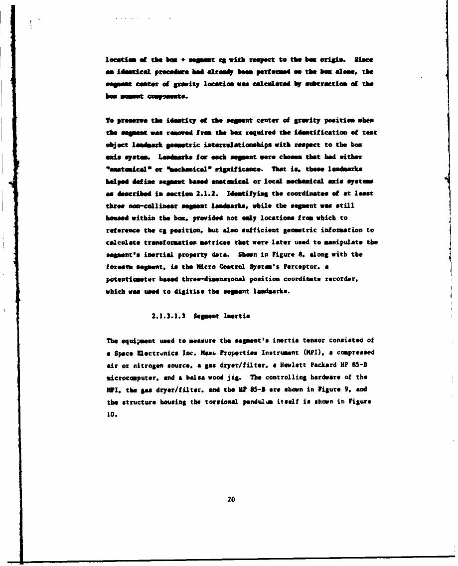
segment's inertial property data. Share in figure 8. along with the
foresem segment, is the Micro Control Systom's Perceptor. a
patentimnt..r based three-dimensional posit ion coordinate recorder.
which was used to digitize the segment landmarks.
2.1.3.1.3 Segiment Inertia
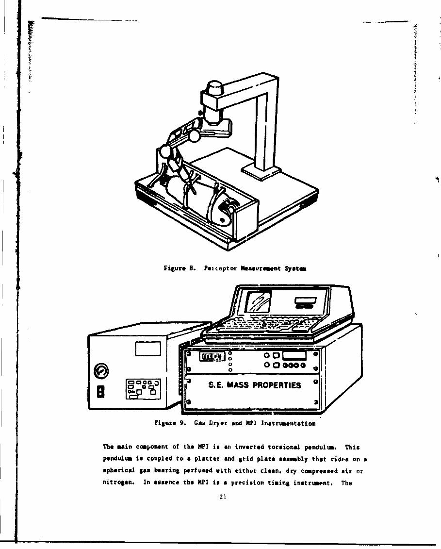
The equipmeat used to measure the segment's inertia tensor consisted of
a Space Mectranics Inc. Max&. Properties Instrument (Nfl). a compressed
air or nitrogeni source. a gs dryer/filter. a Hewlett Packard UP 85-B
microcomputier, and a balsa wood jig. The controlling hardware of the
PIl, the gSe dryer/filter, and the UP 65-1 are shown in Figure 9. and
the structure housing the torsional pendulam itself is showm in figure
10.
20
IC30
figure 9. Gas Dryer and KPI Instrumentationi
The main component of the HPI is at, inverted torsional pendulum. This
pendulum is coupled to a platter and grid platet assembly that rious on aspherical gas bearing perfused with either clean. dry compresstd air or
nitrogen. In essence the MPI to a precision timing instrumont. The
21
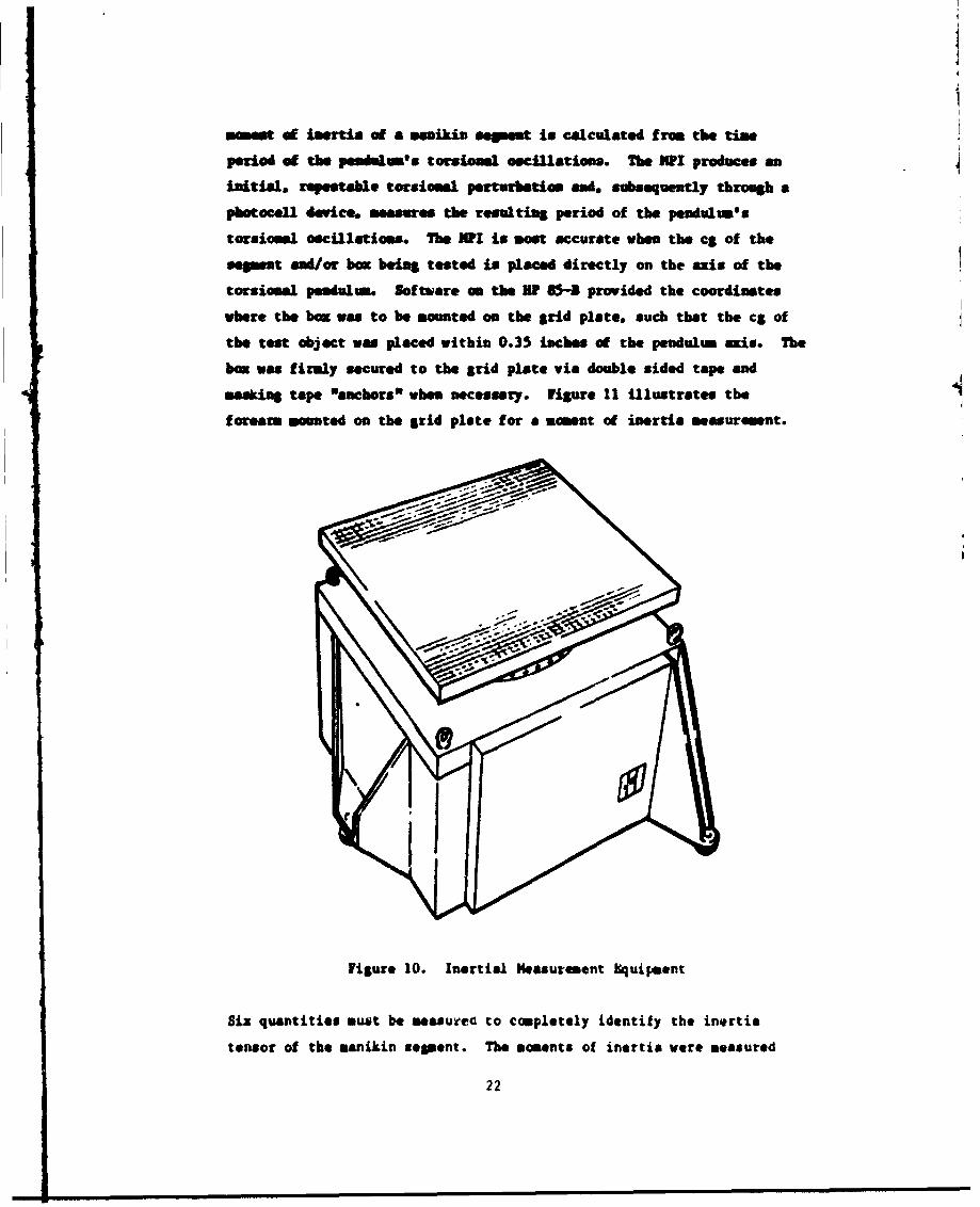
mmet of inertia of a menikin sepient is calculated f rom the time
period ad the penmls torsional oscillations. The NIX produces aninitial, repeatable torsional perturbation made subsequently through aphotocell dewice. mesures the resulting period of the pendulum's
torsional oscillations. The Nil is soot accurate whem the cg of the
gm it andor hiR being tested is placed directly on the axis of the
torsionmal pendul um. Sf tware on the UP 65-3 provided the coordinates
where the boa was to be mounted on the grid plate, such that the c& of
the test object was placed within 0.35 imches of the pendulum axis. The
box was firmly secured to the grid plate via double sided tape and
maskimg tape "amchors* wham necessay. figure 11 Illustrates the
forearm mounted on the grid plate for a moment of inertia measurmnt.
Figure 10. Inertial Neasuzement Squipment
Six quantities must be mestwa to completely identify the inertia
tensor of the manikin spgent. The momenta of inertia wort measured
22
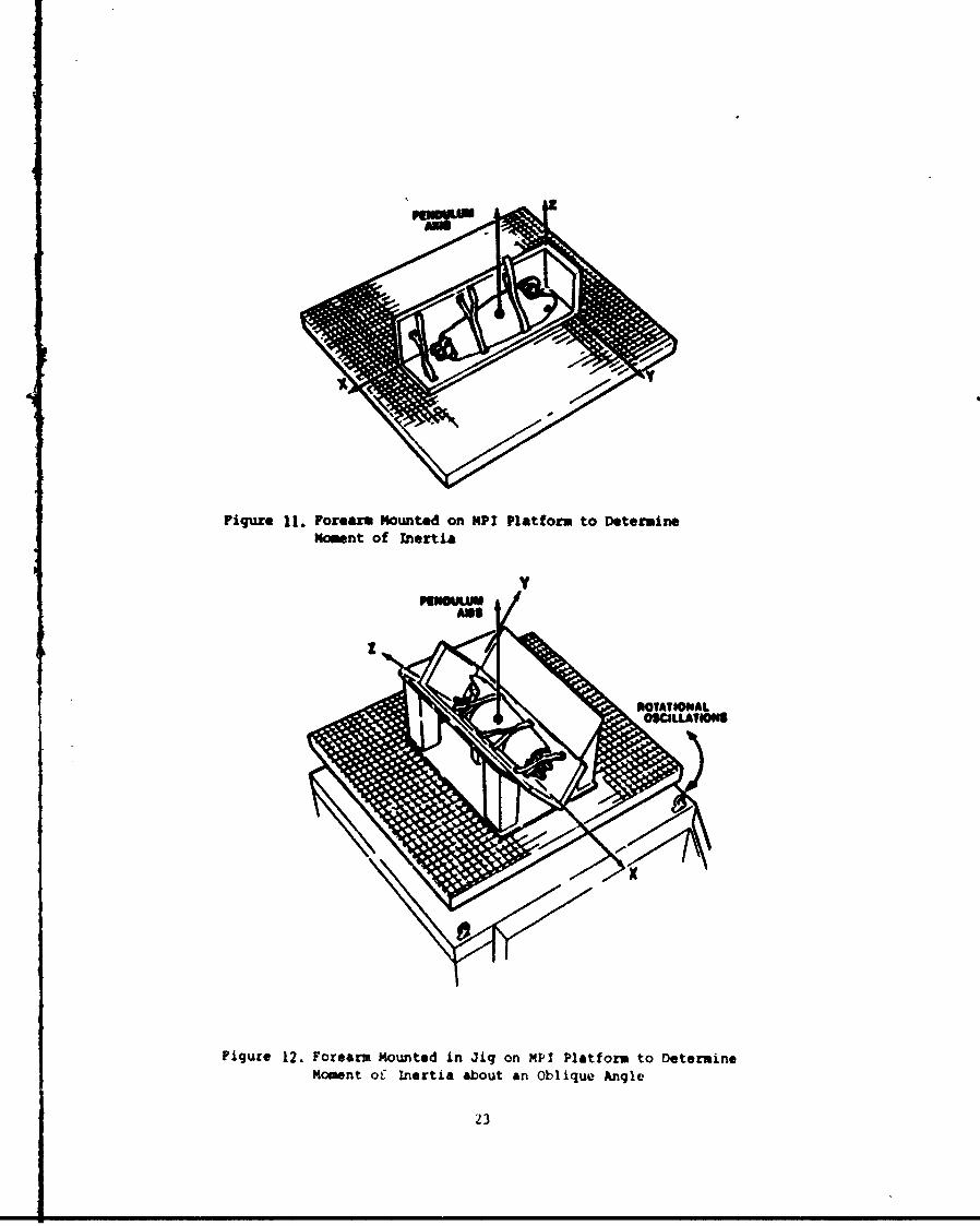
Figure 1.Forearm Mounted on NP! Platform to DetermineMoment of Inertia
Figure 12. Forearm Mounted in Jig on NP! Platform to DetermineMoment of Inertia about an Oblique Angle
23
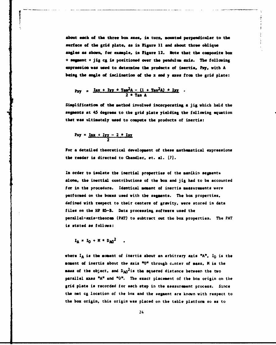
about each of the three box sxes. in turn. mounted perpendicular to the
surface of the grid plate, as in Figure 11 and about three oblique
angles as shown, for eample. in figure 12. Note that the composite box
+ ssaent * jig cg is positioned over the pendulum axis. The following
expression was used to detexine the products of inertia, Pty, with A
being the angle of inclination of the x and y axes from the grid plate:
pay = I +,Iv * T 2A - 1 +T Lg *2 * Tan A
Simplification of the method involved incorporating a j ig which held the
sepnts at 45 degrees to the grid plate yielding the following equation
that was ultimately used to compute the products of inertia:
ay = Iz* + Ivy - 2 * Iy2
For a detailed theoretical development of these mathematical expressions
the reader is directed to Chandler. at. al. (7].
In order to isolate the inertial properties of the manikin segments
alone, the inertial contributions of the box and jig had to be accounted
for in the procedure. Identical moment of inertia measurements were
perforued on the boxes used with the segments. The box properties.
defined with respect to their centers of gravity, were stored in data
files on the liP 85-5. Data processing software used the
parallel-axis-tbeorm (PAT) to subtract out the box properties. The PAT
is stated as follows:
I A z I0 + 1M* DAO2
where IA is the moment of inertia about an arbitrary axis "A", I0 is the
moment of inertia about the axis *0 through cvnter of mass. M is the
ms of the object, and DAo 2 is the squared distance between the two
parallel axes OAO and "0. The exact placement of the box origin on the
grid plate is recorded for each step in the seasurament process. Since
the net cg location of the box and the segment are known with respect to
the box origin, this origin was placed on the table platforu so as to
24
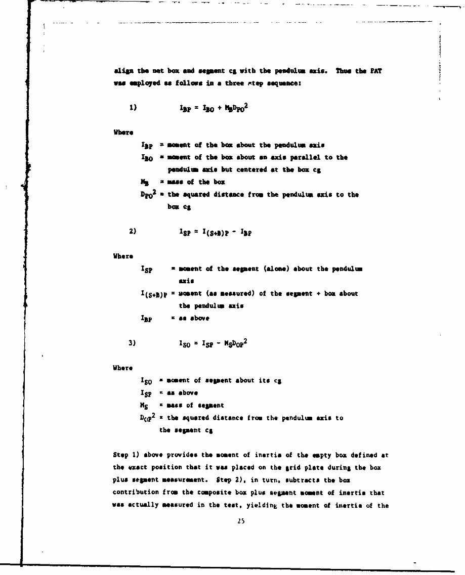
alin the net box and segment cS with the pendulum axis. Thus the PAT
was employed as folloue in a three mtep sequence:
1) ISP= Iso + vso
Where
Illp = moment of the boa about the pendulum axis
ISO a moment of the box about an axis parallel to the
pendulum axis but centered at the box c$
% xmas of the box
DpO2 a the squared distance from the pendulum axis to the
bou c&
2) Isp = I(s B)p- ip
Where
Isp a moment of the segment (alone) about the pendulum
axis
I(S+B)p x moment (as measured) of the segment + box about
the pendulum axis
Isp x as above
3) 'so = ISP - NSDOP2
Where
ISO x moment of segment about its cg
ISp = as above
HS a mass of segment
D¢,p2 x the squared distance from the pendulum axis to
the segment ca
Step 1) above provides the moment of inertia of the empty box defined at
the exact position that it was placed on the grid plate during the box
plus segment measurement. Step 2). in turn. subtracts the box
contribution from the composite box plus segment moment of inertia that
wus actually measured in the test. yielding the moment of inertia of the
25
-, ,- -P- -~ -----
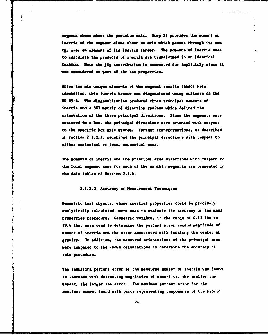
segment, alone about the pendult. axis. Step 3) provides the moment of
Inertia of the segment alone about a axis which passes through its own
eg, L~e. anelement of its inertia teaser. Mwe momenta of inertia used
to calculate the products of inertia are transformed in an identical
fashion. Note the jig contribution is accounted for implicitly since it
wum considered as part of the box properties.
After the six unique elements of the segment inertia tensor were
identified. this inertia tensor was diagonalized using softwate on the
5P 85-D. The diagovlisation produced three principal moments of
inertia and a 3X3 mtrix of direction cosines which defined the
orientation of the three principal directions. Since the segments were
measured in a box, the principal directions were oriented with respect
to the specific box axis system. further transformations, as described
in section 2.1.2.3, redefined the principal directions with respect to
either anatomical or local mechanical "ae.
The moments of inertia and the principal axes directions with respect to
the local #"mot wxe# f or each of the manikin segments are presented in
the data tables of Section 2.1.6.
2.1.3.2 Accuracy of Measurement Techniques
Geometric test objects, whose inertial properties could be precisely
analytically calculated, were used to evaluate the accuracy of the mss
properties procedure. Geomtric weights. in the ran-.@ of 0.15 lbs to
19.6 lbs. were used to determine the percent error versus m.1initude of
mmat of inertia and the error associated with locating the center of
gravity. XIn addition, the measured orientations of the principal axes
were compared to the known orientations to determine the accuracy of
this procedure.
The resulting percent error of the measured moment of inertia ws found
to increase with decreaing magnitude& of moment or, the smaller the
moment, the larg~er the error. The maximum percent errur for the
smallest moment found with pifts representing componetits of the Hybrid
26
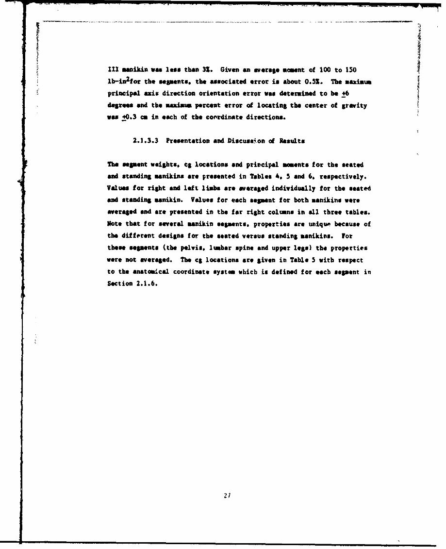
III manikin was less than 3M. Given an average moment of 100 to 150
lb-in2for the segments, the associated error is about 0.51. The maximum
principal axis direction orientation error was determined to be +6
degrees and the maximum percent error of locating the center of gravity
was 40.3 cm in each of the coordinate directions.
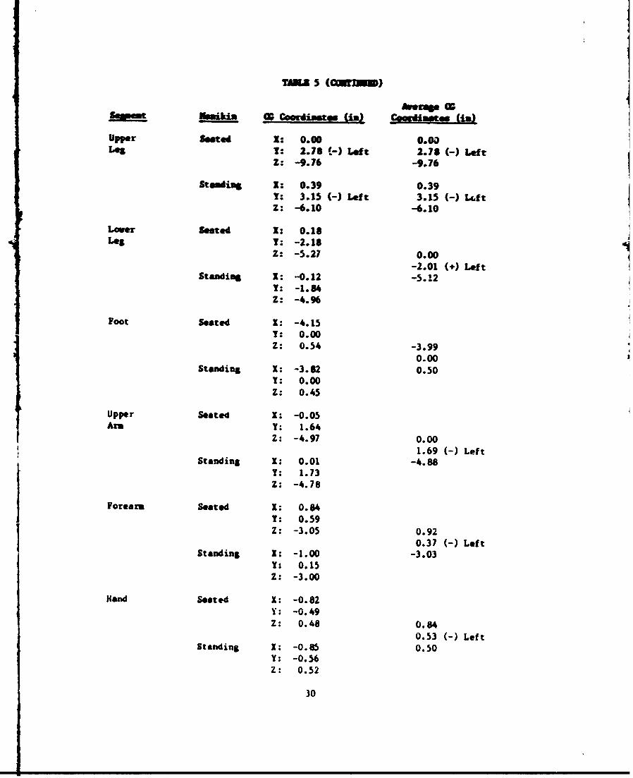
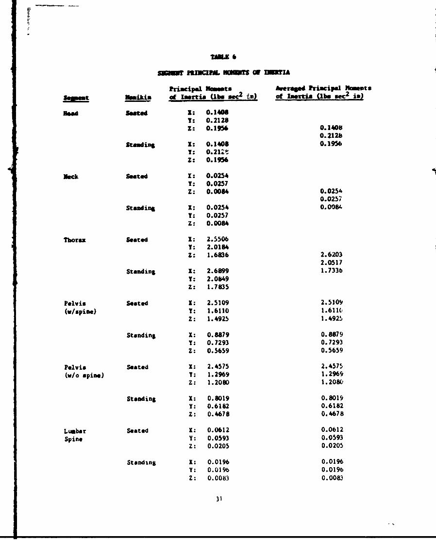
2.1.3.3 Presentation and Discussion at Results
The sesent weights, eg locations and principal moments for the seated
and standing manikins are presented in Tables 4. 5 and 6. respectively.
Values for right and left limbs are averaged individually for the seated
and standing manikin. Values for each segment for both manikins were
averaged and are presented in the far right columns in all three tables.
Note that for several manikin segments. properties are unique because of
the different designs for the seated versus standing manikins. for
these segments (the pelvis, lumbar spine and upper legs) the properties
were not averaged. The cg locations are given in Table 5 with respect
to the anatomical coordinate systm whicb Ls defined for each segment in
Section 2.1.6.
27
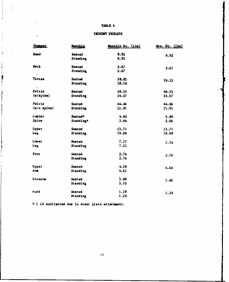
TABLE 4
SEGMET WEIGHTS
Manikin Wt. (1.s) Ave. Wt. (lbs)
Head Seated 9.92 9.92Standing 9.92
Neck Seated 2.67 2.67Standing 2.67
Thorax Seated 38.85 39.22Standing 39.58 2
Pelvis Seated 49.35 49.35(V/Spine) Standing 24.57 24.57
Pelvis Seated 44.46 44.46(L/O spin) Standing 21.91 21.91
Lumber Seated* 4.89 4.89Spine Standing* 2.66 2.66
Upper Seated 13.71 13.71Leg Standing 19.98 19.98
LoUer Seated 7.27 7.64Leg Standing 7.21
Foot Seated 2.76 2.76Standing 2.76
Upper Seated 4, 59 4.60Arm St anding 4.61
korearn Seated 3. S9 3.80Standing 3.70
Iknd Seated 1.29 1.29Standing 1.29
* I lb subtracted due to steel plate attachsent.
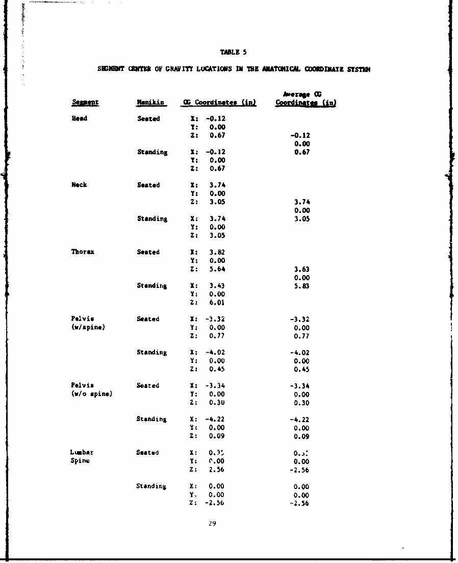
TABLE 5
SEMHDT CMU OF GRAVITY LOCATIONS IN WE ATHICAL COOMDINME SYSTUB
Aveae WSeAmet Manikin Q; Coordinat , (in) Coodiae (b)
ead Seated 1: -0.121: 0.00Z: 0.67 -0.12
0.00Standin 1: -0.12 0.67
y: 0.00Z: 0.67
Neck Seated 1: 3.74Y: 0.00Z: 3.05 3.74
0.00Standing X: 3.74 3.05
Y: 0.00Z: 3.05
Thorax Seated 1: 3.82Y: 0.00Z: 5.64 3.63
0.00Standi,8 X: 3.43 5.83
Y: 0.00Z: 6.01
Pelvis Seated X: -3.32 -3.32(v/spine) Y: 0.00 0.00
Z: 0.77 0.77
Standing X: -4.02 -4.02Y: 0.00 0.00Z: 0.45 0.45
Pelvis Seated X: -3.34 -3.34(v/o spine) Y: 0.00 0.00
Z: 0.30 0.30
Standing X: -4.22 -4.22Y-0 0.00 0.00Z: 0.09 0.09
Liumbr Seated X: .13 O..Spine Y: P.00 0.00
Z: 2.56 -2.56
Standing X-: 0.00 0.00Y'. 0.00 0.00Z: -2.56 -2.56
29
TAK4 5 (rM )
Upper Seated 1: 0.00 0.00LOg 1: 2.78 C-) Left 2.78 (-) Left
Z: -9.76 -9.76
Standin 1: 0.39 0.39Y: 3.15 (-) Left 3.15 (-) LeftZ: -6.10 -6.10
Lower Seated X: 0.18Let Y: -2.18
Z: -5.27 0.00-2.01 (+) Left
Steading X: -0.12 -5. 12Y: -1.84Z: -4.96
Foot Seated K: -4.15Y: 0.00Z: 0.54 -3.99
0.00Stding X: -3.62 0.50
T: 0.00Z: 0.45
Upper Seated 1: -0.05Ara Y: 1.64
Z: -4.97 0.001.69 (-) Left
Standing 1: 0.01 -4.88Y: 1.73Z: -4.78
Forearm Seated 1: 0.841: 0.59Z: -3.05 0.92
0.37 (-) LeftStanding 1: -1.00 -3.03
Y: 0.15
Z: -3.00
Hand Seated X: -0.82Y: -0.49Z: 0.48 0.84
0.53 (-) LeftStanding 1: -0.85 0.50
Y: -0.56Z: 0.52
30
TA"I. 6
- PWIU 0 S M 11 f WIA
ft'isipal Aiucipal Mmnt
Mwikin nri Uesm p of Inertia (lb. Ze2 ij)
ed Seated 1: 0.1406T: 0.2128Z: 0.1956 0.1408
0. 212b8Standing X: 0.1408 0.1956
I: 0.214Z: 0.1956
Meck Seated 1: 0.0254T: 0.0257Z: 0.0084 0.0254
0.0257
Standing 1: 0.0254 0.008.1: 0.0257Z: 0.0084
Tborax Seated 1: 2.55061: 2.0164Z: 1.6836 2.6203
2.0517Standing 1: 2.6899 1.733b
Y: 2.0849Z: 1.7835
Pelvis Seated I: 2.5109 2.5109(v/spine) 1: 1.6110 1.6111,
Z: 1.4925 1.4925
Standing 1: 0. 879 0.8879Y: 0.7293 0.7293Z: 0.5659 0.5659
Pelvis Seated X: 2.4575 2.4575
(W/O spine) 1: 1.2969 1. 2969Z: 1.2080 1.2080
Standing X: 0.8019 0.8019Y: 0.6182 0.6182Z: 0.4678 0.4678
Lumber Seated X: 0.0612 0.0612Spine Y: 0.0593 0.0593
Z: 0.0205 0.0205
Standing X: 0.0196 0.0196Y: 0.0196 0.0196Z: 0.0083 0.0083
31
TaKs 6 (aMruuU)
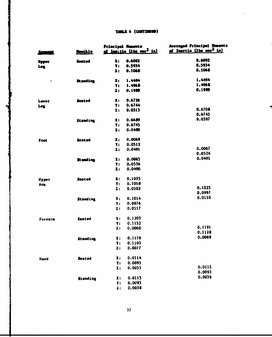
?uimcipa1 Mmnts A.era ?dacipa Now tmmikim d s.. Ube Sa2 i.) of ,inetia Ube SOC 2 in)
Upger Seated 1: O.6092 0.692
Los 1: 0.5934 0.5934Z: 0.1066 0.1068
Standing 1: 1.4494 1.44941: 1.4968 1.496Z: 0.1989 0.1989
Lower Seated 1: 0.6726LeO 1: 0.6744
Z: 0.0313 0.67060.6745
Standing X: 0.6689 0.0397Y: 0.6745Z: 0.048D
Foot Stated 1: 0.00691: 0.0512Z: 0.0491 0.0067
0.0524
Steading 1: 0.0065 0.04911: 0.0536Z: 0.0490
Upper Seated 1: 0.1035Are 1: 0.1018
Z: 0.0102 0.10250.0997
Standing 1: 0.1014 0.0110Y: 0.0976Z: 0.0117
Forearm Seated 1: 0.1203Y: 0.1152Z: 0.0060 0.1191
0.1128
Standing X: 0.1179 0.00691: 0.1103Z: 0.0077
Hand Seated X: 0.0114Y: 0.0093Z: 0.0033 0.0115
0.0093
Standing 1: 0.0115 0.0036
Y: 0.0093Z: 0.0038
32
2.1.4 Measurement of Hanikin Joint Physical Characteristics
In order to properly reflect natural limitations in human joint freedom
of motion, the Hybrid III dmmies have built-in joint stops. While
those stops are structurally yell defined, their effective position can
be seuwbat modified by some local structural deformation and by the
interaction of the soft flesb coverings. Joint resistive properties can
also be modified by applying resistive torque through friction devices
in the manikin joints. This frictional force is user adjutsble and is
mainly used for maintaining constant manikin position prior to the main
impact exposure. In the tests described herein, the net effect of all
the parameters which contribut2 to joint resistive torque were measured
except that of the joint friction mechanism.
2.1.4.1 Measurement of Joint Resis*ance Torque as a Function
of Joint Rotational Angle
The A1/S model joint modeling capability requires the representation
of joint torque resistance a a function of angular rotation. The joint
characteristic testing in this study was designed to provide this data.
In general. the testing approach involved the rigid clamping of one of
two articulated segments, the forcing of the free segment through a
planar arc using a load cell and measuring the force required and the
angle of rotation. Using this process, both for loading and unloading.
resulted in joint load deflection characteristics.
2.1.4.1.1 Description of Joints and Test Set-Up
With the exception of the hip. which has a ball and socket joint, tho
articulations of the shoulder, elbow, wrist, knee, and ankle are pin
jointed devices. For a pin joint, the two clevices of the aojoining
sepects are hinged together by a bolt and washer combination that
provides a planar range of motion with the hardware, stove, or soft
covering determining the particular range of motion. While the joints
13
can be tightened to provide variable joint resistance, all joints within
this study were loosely torqued to slw free range of notion within the
limits of the soft and hard stops.
For a joint under investigation, only the two adjoining segments were
used to conduct the test. One segmnt was clamped solidly to a holding
frame in a manner that would bold the weight of the test object without
intetfering with the range of motion. In addition, the stationary
segment was positioned so that the joint axis was parallel to the
gravity vector to eliminate the effect of the torque about the joint due
to the weight of the rotating segment.
2.1.4.1.2 Instrumentation Utilized
A Waters AK potentiometer and a Strainsert 250 lb single-axis load cell
were used to measure the angle of rotation and the applied force.
respectively. The output of these transducers were fed to a
Hewlett-Packard X - Y recorder. Calibrations of the potentiometer, used
to record joint rotation, indicated that the potentiometer had a 0.1
degree of accuracy and good linearity. The load cell was wired through
a bridge balance and amplifier to the y-axis of the x-y recorder and was
periodically calibrated. The load cell had a 0.75 lb accuracy.
For the loosely torqued joints, the bolt holding the two clevices
rotated through the full range of motion with the movement of the
rotating segment. This rotating bolt was attached directly to the ais
of the potentiometer through an interface fixture which was designed to
fit the head of the box bolt. The load cell was positioned
perpendicular to the limb axis and parallel %ilh the plane of rotational
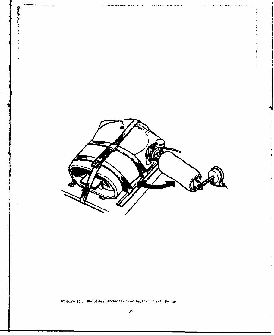
notion. Se, for example, Figure 13. Using "Ae load cell as the force
application device, the free segment was mentally rotated through the
entire range of notion. The resulting force versus angle curve was
recorded on the x-y plutter. The desired torquv versus angle
characteristics were then determired by mesur4.ng the length of the
mobile segment lever aru and multiplying this length by the measured
force.
34
V4
Figure 13. Shoulder Abduct ion- Adduct ion Tt! Ft Setup
Generally, the curve displayed a flat region of joint torque with angle
of rotation within the free rsae of motion, that range which
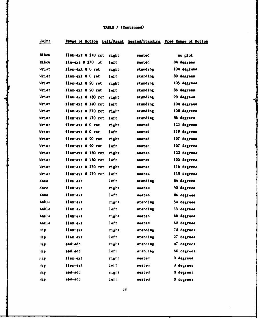
experiences little or no resistance. A summary table of the free range
of motion of each joint is found in Table 7. The interference of soft
covering or soft stops generally increased the resistance in a nonlinear
manner. This nonlinearity further increased as the joint hard stop was
reached. The direction of notion was reversed to measure the unloading
characteristic and the loading characteristic in the opposite direction.
While the polarity of te curves may vary depending on the polarity of
the instrumentation for a particular test, the curves could be compared
by identifying the maximum ranges of notion and the corresponding
applied terquaL.. To define the curves. arrows depict the direction of
loading and unloading of the joint and the extreme ends of the curve are
labeled with extension, flexion, abduction, or adduction. The start
positions are also noted.
2.1.4.1.3 Tests
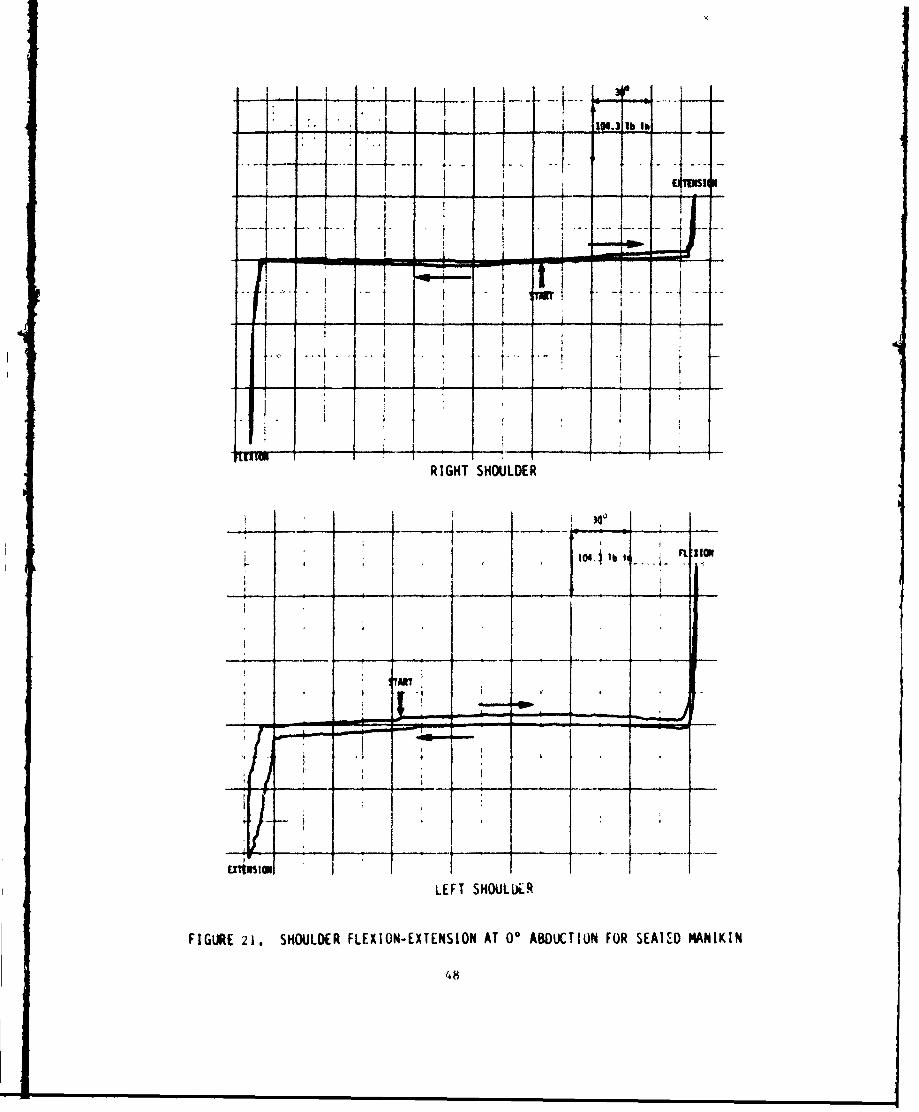
2.1.4.1.3.1 Shoulder
1lexion-extonsion and abduction-adduction movement of the shoulder is
provided by two pin joints. Assuming the upper arm in the anatomical
position. (hanging vertically down with the long bone axis parallel to
the mid-sagittal plane). flezion-extension notion is obtained by
rotating the arm forward and backward while remaining parallel to the
sid-saggital plane. Again assuming the anatuaical position.
abduction-adduction motion is obtained by rotating the upper ars way
from and toward the body while remaining within the frontal plane.
nlexion-xtension characteristics were tested with initial abduction
angles of 0 and 45 degrees. The angles were approximated with the aid
of a goniomter and the abduction-adduction pin joint was tightly
torqued to hold this positio. Abduction-adduction tests were performed
with 0 at' 90 degrees ot flexion.
Abduction-adduction angle ot rotation of 00 flexion was measured by
first positioning the upper torso horizontally and holding it securely
36
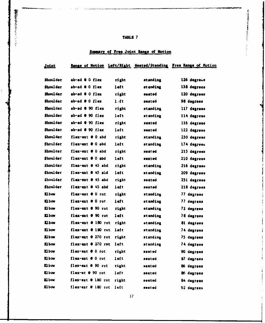
TABLE 7
Sumary of Free Jobnt !~Mae of Notion
Joints of Notion Left/Right Seated/Standins Free Rane of Motion
Shoulder sb-ad 0 0 flex right standing 126 degreus
Shoulder 8b-ad 0 0 flex left standing 138 degrees
Shoulder 8b-sd 0 0 flex right seated 120 degrees
Shoulder sb-ad 0 0 flex l..ft seated 98 degrees
Shoulder ab-ad 0 90 flex right standing 117 degrees
Shoulder ab-ad 0 90 flex left standing 114 degrees
Shoulder sb-ad S 90 flex right seated 116 degrees
Shoulder ab-ad 0 90 flex left seated 122 degrees
Shoulder flex-ext 0 0 abd right standing 230 degrees
Shoulder flex-ext 0 0 sbd left standing 174 degrees
Shoulder flex-eat S 0 abd right seated 215 degrees
Shoulder flex-ext 0 0 abd left seated 210 degrees
Shoulder flex-ext & 45 abd right standing 216 degrees
Shoulder flex-eat 0 45 ad left standing 209 degrees
Shoulder flex-ext 0 45 ebd right seated 251 degrees
Shoulder flex-eat 0 45 abd left seated 218 degrees
Elbow flex-ext 0 0 rot right standing 77 degrees
Elbow flex-ext 0 0 rot left standing 77 degrees
Elbow flex-ext @ 90 rot right standing 72 degrees
Elbow flex-ext 0 90 rot left standing 78 degrees
Ilbow flex-ext * 180 rot right 6tanding 81 degrees
Elbow flex-ext # 100 rot left standing 74 degrees
Elbow flex-eat 0 270 rot right standing 75 degrees
Elbow flex-ext 0 270 rot left standing 74 degrees
Elbow flex-ext # 0 rot right seated 90 degrees
Elbow flex-ext 0 0 rot left seated 87 degrees
Elbow flex-ext • 90 rot right seated 86 degrees
Elbow flex-st @ 90 rot left seated 86 degrees
Elbow flex-ezt 0 180 rot right seated 84 degrees
Elbow flex-ext @ 180 rot left seated 92 degree.
37
TADLIS 7 (Continued)
Joint IMng Of Notion Let t/Riabt Seated/Standita free Range of Notiont
Elbow flex-ext 0 270 rot right seated no plot
Elbow fie-ext 0 270 -2 lef t Seated 84 degrees
Wrist flex-ext * 0 rot right standing 104 degrees
Wrist flex-ext 0 0 rot left standing 89 degrees
Wrist flex-ext 0 90 rot right standing 105 degrees
Wrist flex-ext 090o rot left standing 86 degrees
Wrist flex-ext 0 180 rot right standing 99 degrees
Wrist flex-ext 0 180 rot left standing 104 degrees
Wrist flex-ext 6 270 rot right standing 108 degrees
Wrist flex-ext 0 270 rot left standing 86 degree.
Wrist flex-ext 0 0 rot right seated 123 degrees
Wrist flex-ext 0 0 rot left seated 119 degrees
Wrist flex-eat 0 90 rot right seated 107 degrees
Wrist flex-ext 6 90 rot left seated 107 degrees
Wrist flex-ext *@180 rot right seated 122 degrees
Wrist flex-ext 0 IS0 rot left seated 105 degrees
Wrist flex-ext & 270 rot right seated 116 degrees
Wrist flex-ext 0 270 rot left seated 119 degrees
Knee flex-ext left standing 84 degrees
Knee flex.-ext right seated 90 degrees
Knee flex-ext left Seated 86 degrees
Ankle flex-eat right standing 54 degrees
Ankle flex-ext left standing 33 degrees
Ankle flex-ext right seated 66 degrees
Ankle flex-ext left seated 68 degrees
Hip flex-ext right standing 78 degrees
Hip flex-ext left standing 27 degrees
Hip abd-sdd right standing 47 degrees
Hip abd-add left standing 60 degress
Hip flex-ext right seated 0 degrees
Hip flex-ext left seated 0 degrees
Hip abd-add right seated 0 degrees
Hip abd-add left seated 0 degrees
38
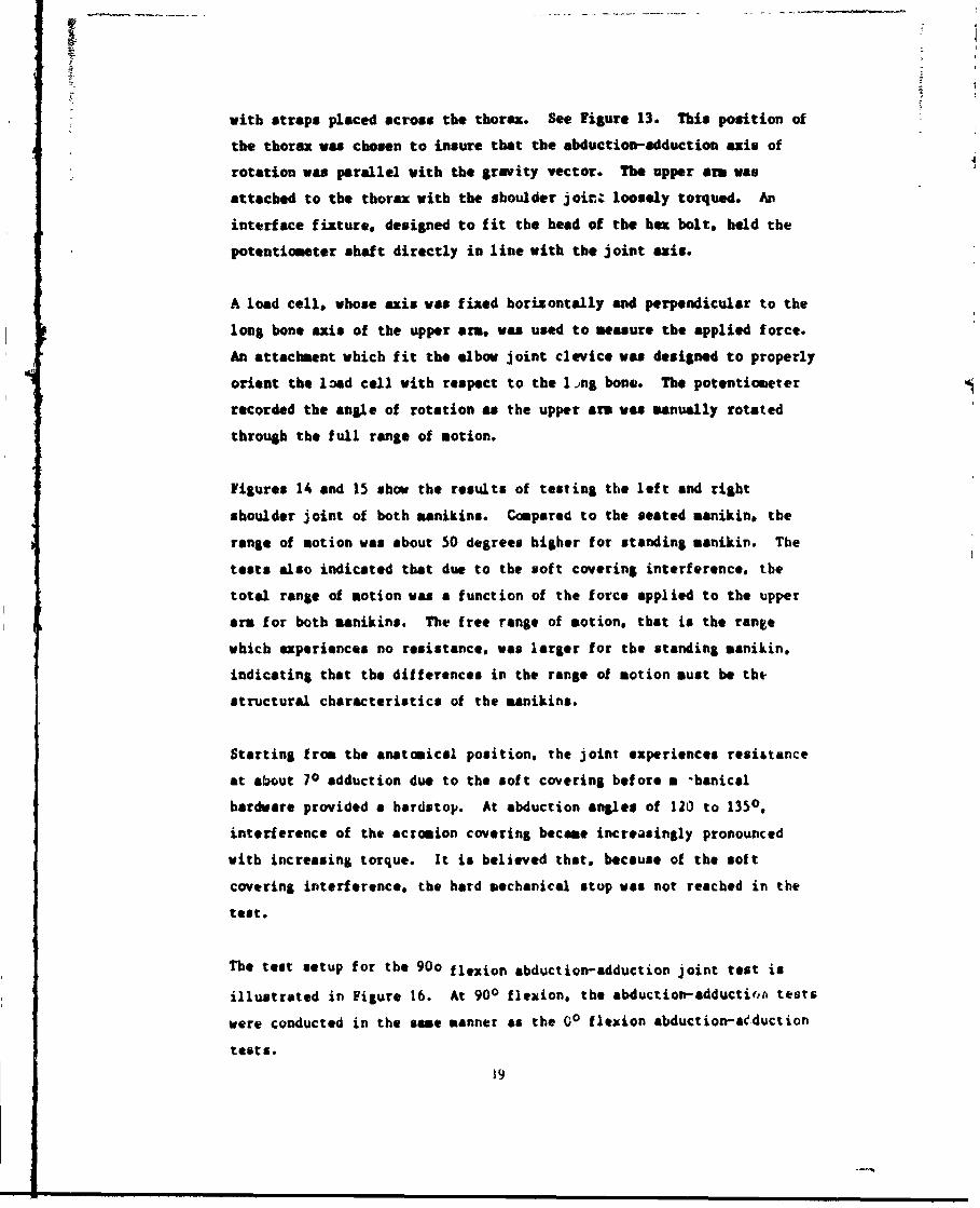
kwith straps placed across the thorax. See figure 13. This position of
the thorax was chosen to insure that the abduction-adduction axis of
rotation was parallel with the gravity vector. The upper am was
attached to the thorax with the shoulder joiz loosely torqued. An
interface fixture, designed to fit the head of the hex bolt, held the
potentiometer shaft directly in line with the joint ais.
A load cell. whose axis was fixed horizontally and perpendicular to the
long bone axis of the upper am. was used to measure the applied force.
An attachment which fit the elbow joint clevice was designed to properly
orient the load cell with respect to the 1 .ng bone. The potentiometer
recorded the angle of rotation as the upper arm was manually rotated
through the full range of motion.
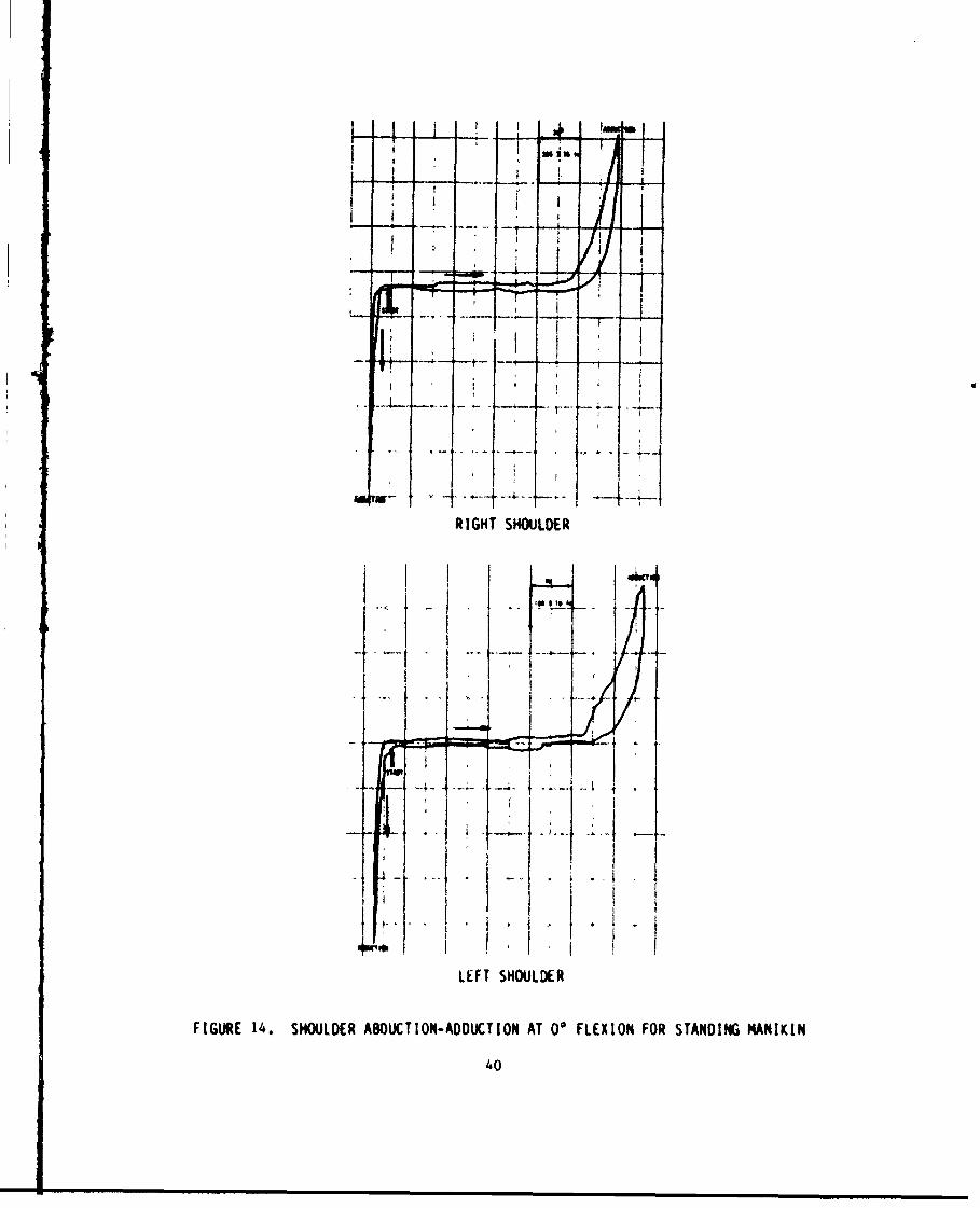
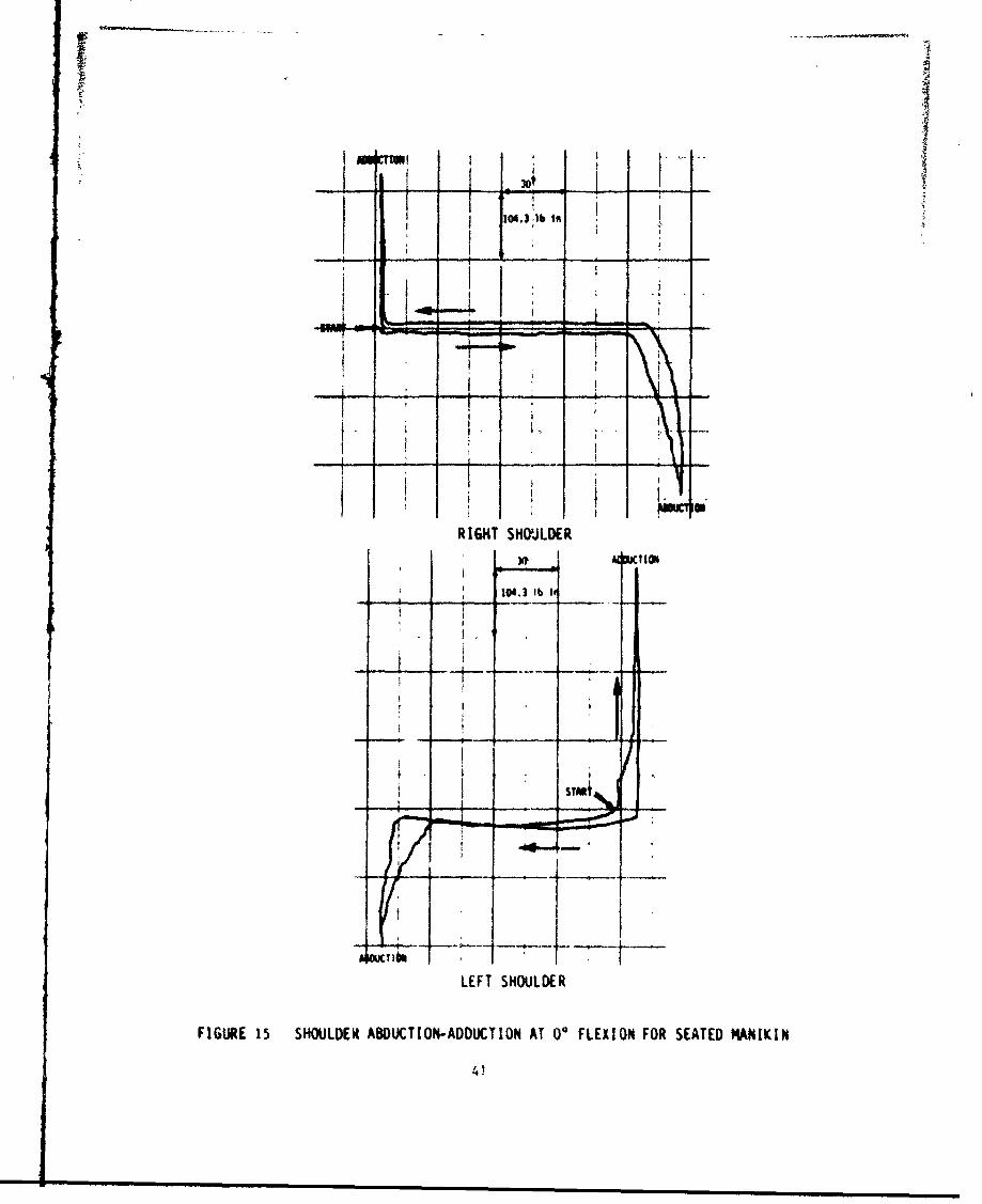
Figures 14 and 15 show the results of testing the left and right
shoulder joint of both manikins. Compared to the seated manikin, the
range of motion was about 50 degrees higher for standing manikin. The
tests also indicated that due to the soft covering interference, the
total range of motion was a function of the force applied to the upper
arm for both manikins. The free range of motion, that is the range
which experiences no resistance, was larger for the standing manikin.
indicating that the differences in the range of notion must be the
structural characteristics of the manikins.
Starting from the anatomical position, the joint experiences resistance
at about 70 adduction due to the soft covering before a -hanical
hardware provided a hardstop. At abduction angles of 120 to 1350.
interference of the acromion covering became increasingly pronounced
with increasing torque. It is believed that, because of the soft
covering interference, the hard mechanical stop was not reached in the
test.
The test setup for the 900 flexion abduction-adduction joint test is
illustrated in Figure 16. At 900 flexion. the abduction-adductiro tests
were conducted in the same manner as the 0o flexion abduction-aeduction
tests.
)9
RIGHT SHOULDER
40
zL f -ii -.-
RIGHT SHOUI R
t . TI.
104.3 lb It
' I )
itm
LEFT SHOULDER
FIGURE 15 SHOULDER ABDUCTION-ADDUCTION AT 0 FLEXION FOR SEATED MANIKIN
41
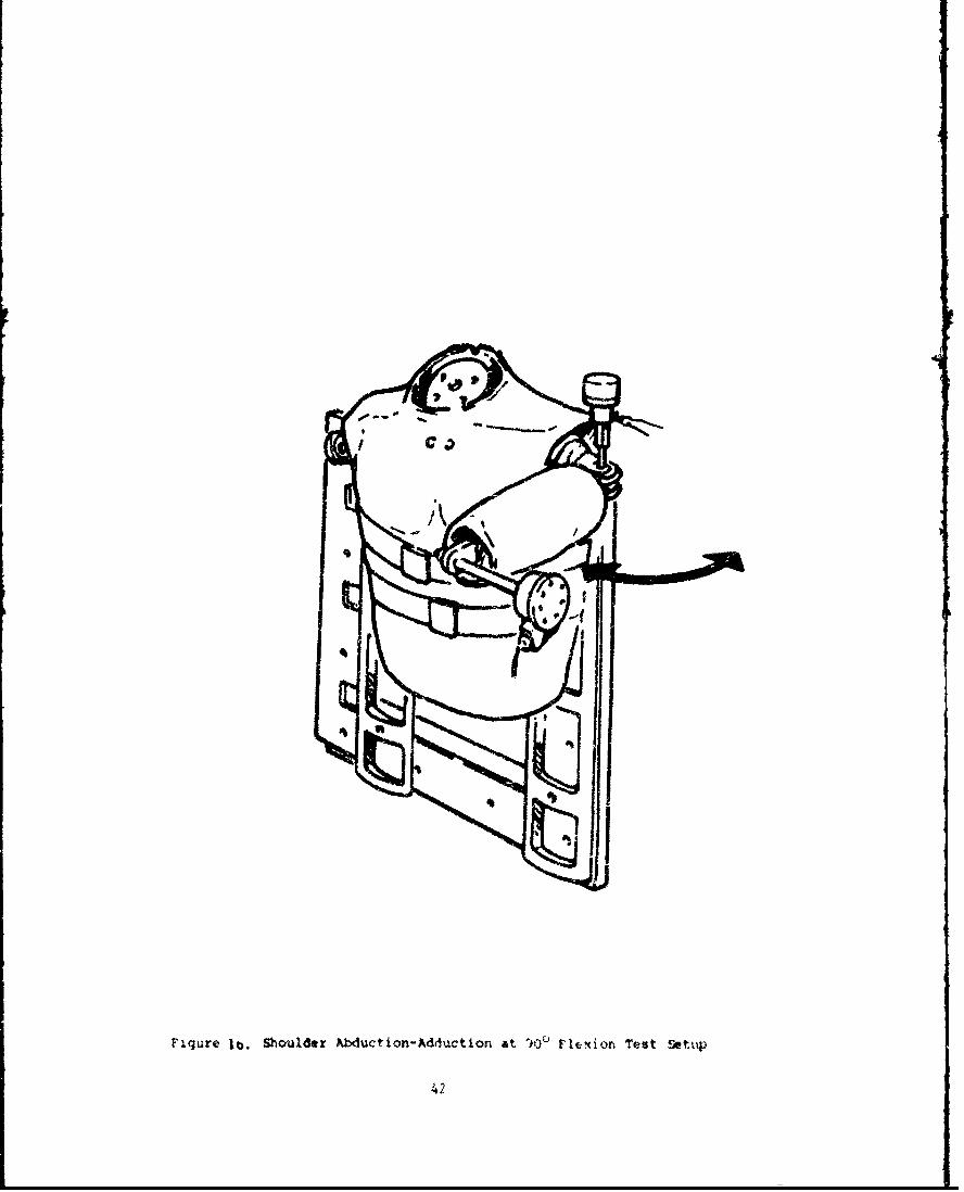
Figure lb. Shoulder Auction-Adductio-. At ')OU Fleio Test Settup
42
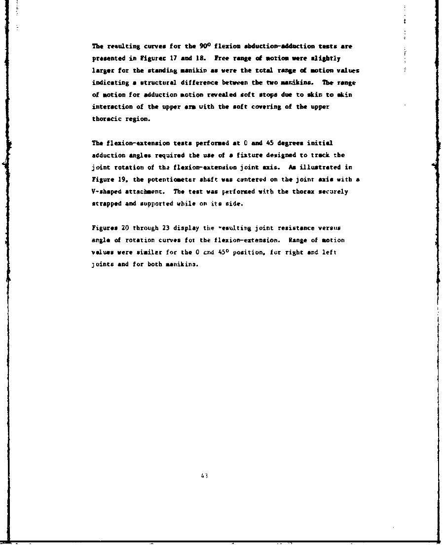
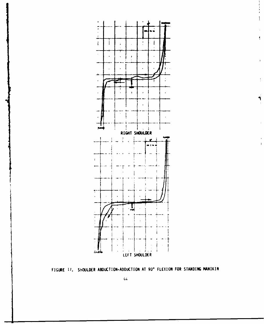
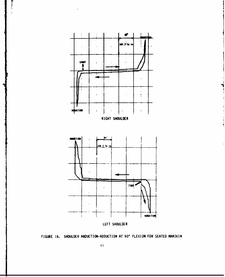
The resulting curves for the 900 flexion abductioo-adductiou tests are
presented in Figuret 17 and 18. Free range of motion were sligbtly
larger for the standing manikin as were the total rafne of motion values
indicating a structural difference between the two marAkins. The range
of notion for adduction motion revealed soft stops due to skin. to skin
interaction of the upper aun with the soft covering of the upper
thoracic region.
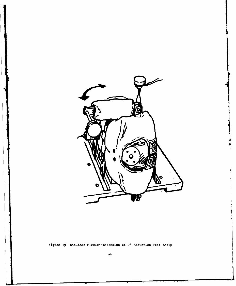
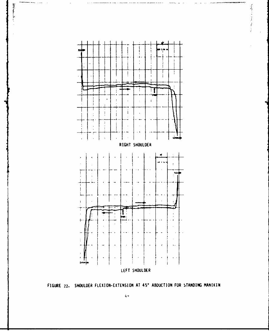
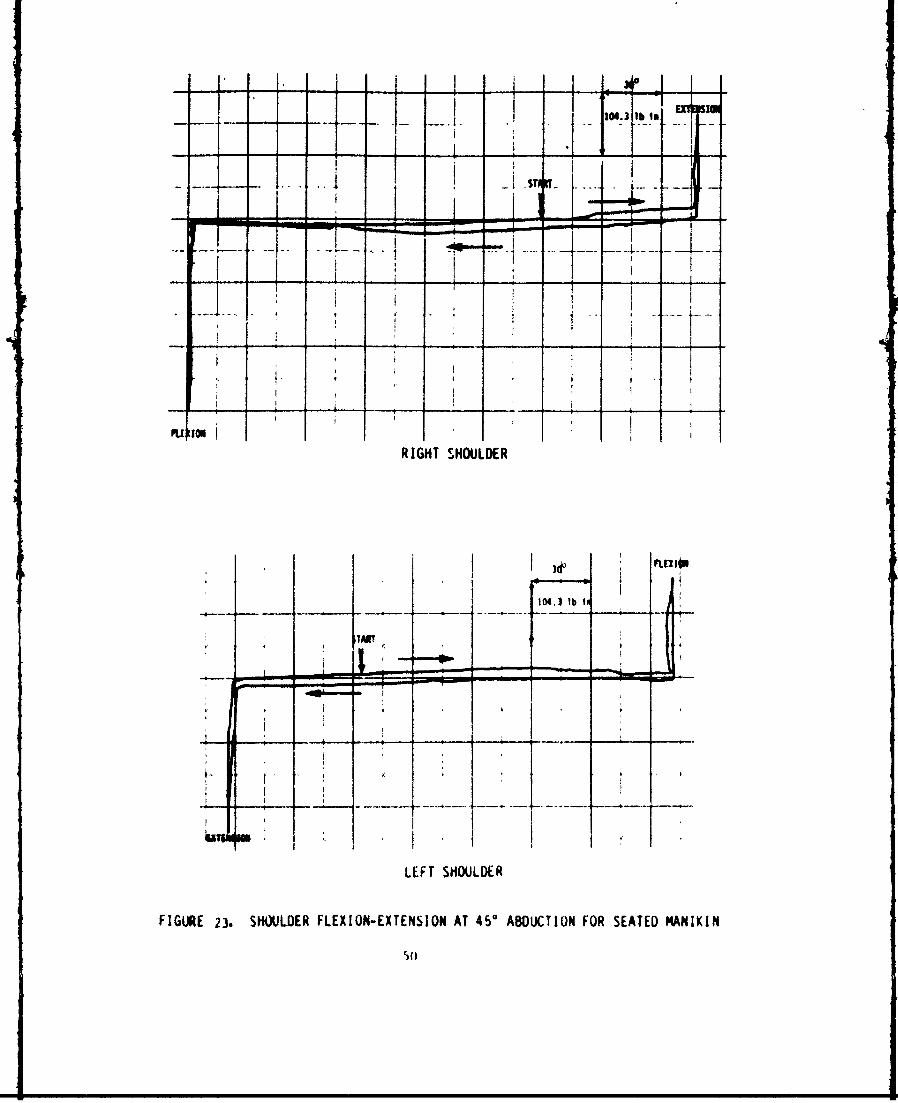
The flexion-extension tests perforued at 0 and 45 degrees initial
adduction angles required the use of a fixture designed to track the
joint rotation of the flexion-extensios joint axis. As illustrated in
Figure 19. the potentiometer sh&fr was centered on the joint axis with a
V-shaped attachment. Th. test was pgrfomed with the thorax securely
strapped and supported while on its side.
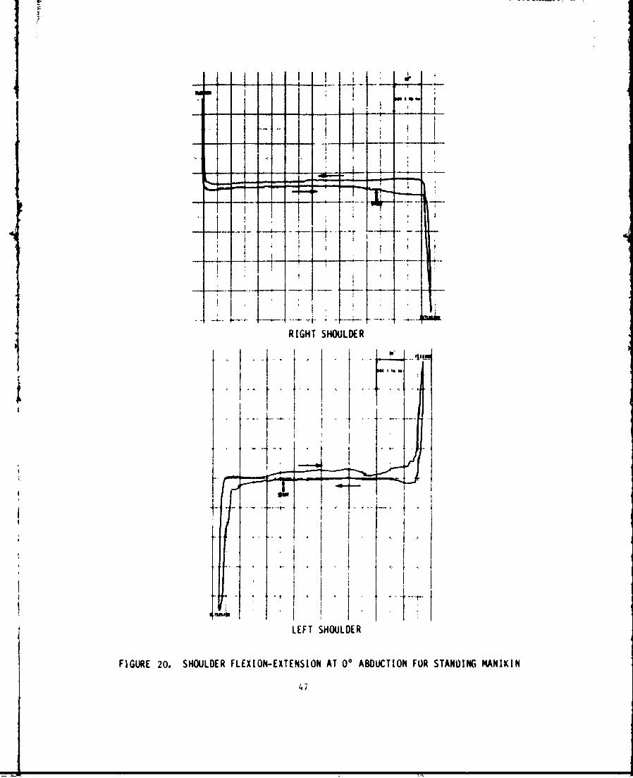
Figures 20 through 23 display the -esulting joint resistance versts
angle of rotation curves foi the flexion-extension. Range of motion
values were similar for the 0 cr4 450 position, for right and left
3oints and for both manikins.
43
* 1
RIGHT SHOULDER
H--- 1
*
sLEFT SHOULDER
FIGURE 11. ShOtLDER ABDUCTION-AD$CTION AT 900 FLEXION FOR STANDING MANIKIN
44
Sim
S- --
RIGHT SHOULDER
104 1 lb in
LEFT SHOULDER
FIGURE 18. SHOULDER ABHUCTION-ADDUCTION AT 90 FLEXION FOR SEATED NIKN
45
%I
Fique 1. Shuldr Fexio- Ftensionat 0 Abucton Tst etC464
SI I.... i
. ~ ~-- . __ ,.. ..
-- I- -
RIGHT SHOULDER{ -I' f- 1'±4'
.. I.. -
LEFT SHOULDER
FIGURE 20. SHOULDER FLEXION-EXTENSION AT 0° ABDUCTION FOR STANOING IMANIKIN
4;
, .)l. u _ _ _I ..... -.. -"
I .I t
1- . t II1.1
-4 I -, -
RIGHT SHOULDER
104. b ... FUSION
. .i - 4..
- -I - ,---i
LEFT SHOULLU
FIGURE 21. SHOULDER FLEXION-EXTENSION AT 0* ABDUCTION FOR SEALED MANIKIN
48
R4-
, , 1 T, T
±twiVK' "RIGHT SHOULDER
I _
- .. . ' I * "
LEFT SHOULDER
FIGURE 22. SHOULDER FLEXION-EXTENSION AT 45* ABDUCTION FOR STANDING MANIKIN
4q
S IT' , .3 lbis--... I --. .L __.HI
- 1 1/4
i t --J-2
Ing
t 4 *.... . . .
RIGHT SHOULDER
I04,1 lb I
-4---- -,---- - - -.. - ---- -
I - ' _ _ _
FIGURE 23. SHOULDER FLEXION-EXTENSION AT 450 ABDUCTION FOR SEATED MANIKIN
50 _-
IiI
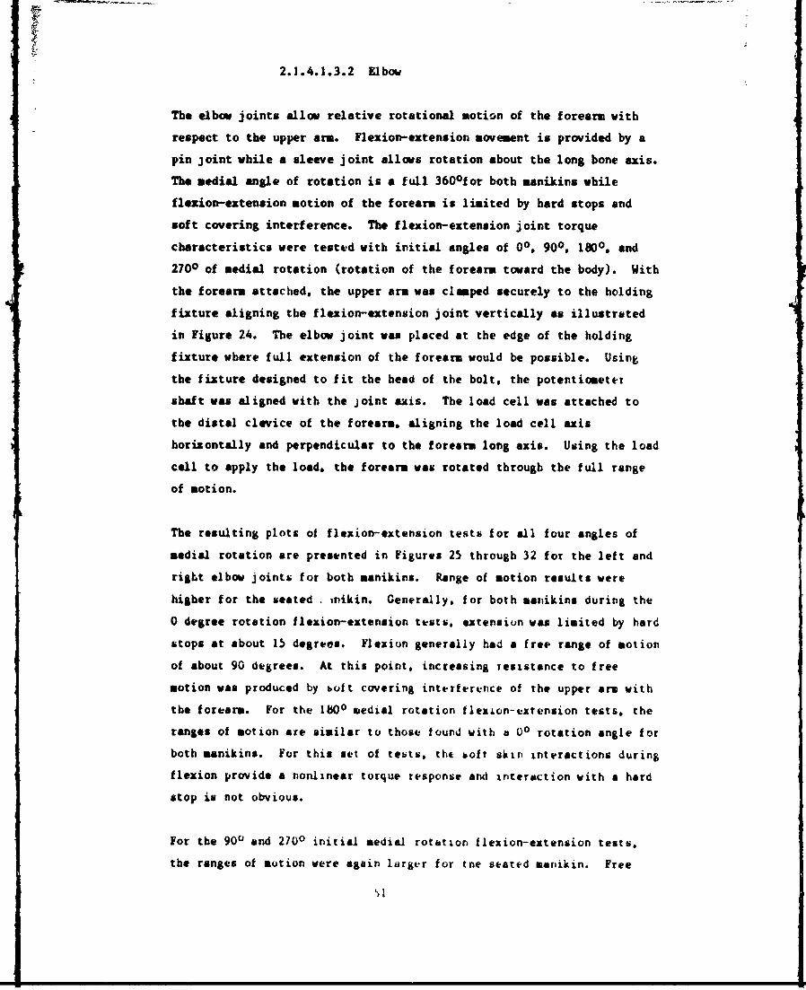
2.1.4.1.3.2 Elbow
The elbow joints allow relative rotational motion of the forearm with
respect to the upper arm. Flexion-extension movement is provided by a
pin joint while a sleeve joint allows rotation about the long bone axis.
The medial angle of rotation is a full 360 0 for both manikins while
flexion-extension motion of the forearm is limited by hard stops and
soft covering interference. The flexion-extension joint torque
characteristics were tested with initial angles of 00. 900. 1800. and
2700 of medial rotation (rotation of the forearm toward the body). With
the forearm attached, the upper arm was clamped securely to the holding
fixture aligning the flexion-extension joint vertically as illustrated
in Figure 24. The elbow joint was placed at the edge of the holding
fixture where full extension of the forearm would be possible. Using
the fixture designed to fit the head of the bolt. the potentiometer
shaft was aligned with the joint axis. The load cell was attached to
the distal clevice of the forearm, aligning the load cell axis
horizontally and perpendicular to the forearm long axis. Using the load
call to apply the load, the forearm was rotated through the full range
of motion.
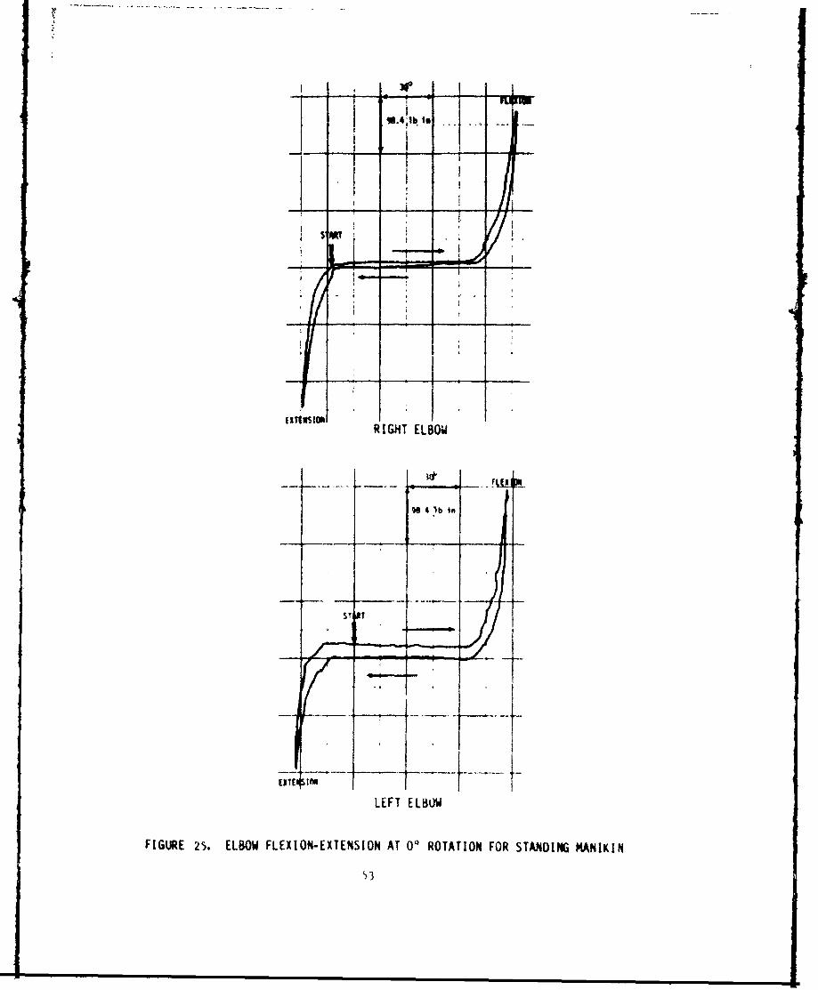
The resulting plots of flexion-extension tests for all four angles of
medial rotation are presented in Figures 25 through 32 for the left and
right elbow joints for both manikins. Range of motion results were
higher for the seated .nikin. Generally. for both manikins during the
0 degree rotation flexion-extension tests, extension was limited by hard
stops at about 15 degrees. Flexion generally had a free range of motion
of about 90 degrees. At this point, increasing resistance to free
motion was produced by bot covering interference of the upper arm with
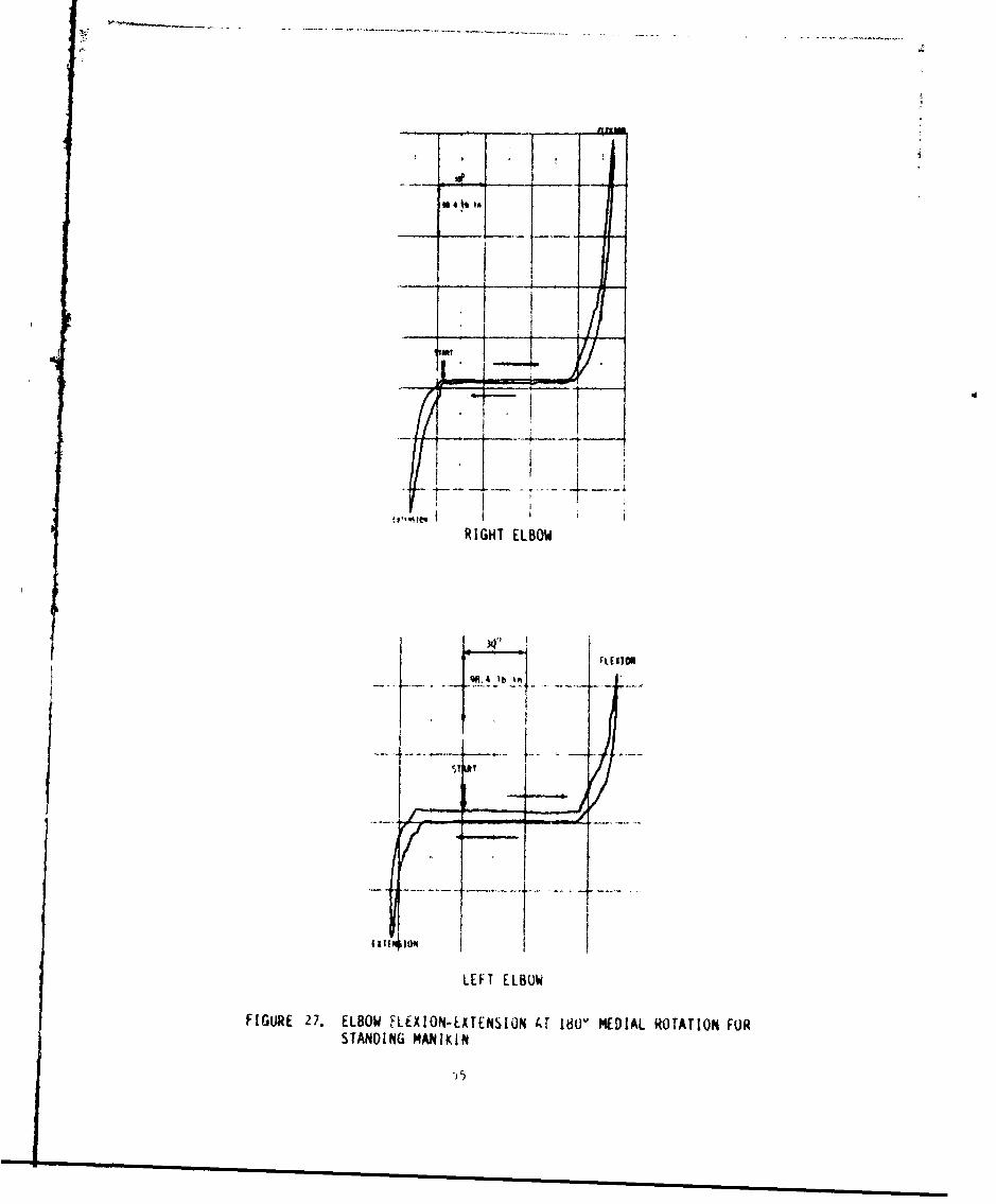
the forearm. For the 180 0 medial rotation flexion-extension tests, the
ranges of motion are similar to those found with a 00 rotation angle for
both manikins. For this set of tests, tht soft skin interactions during
flexion provide a nonlinear torque response and interaction with a hard
stop is not obvious.
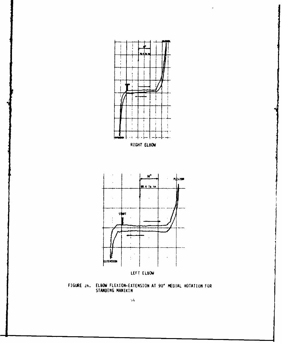
For the 900 and 2700 initial medial rotation flexion-extension tests.
the ranges of notion were again larger for the seated manikin. Free
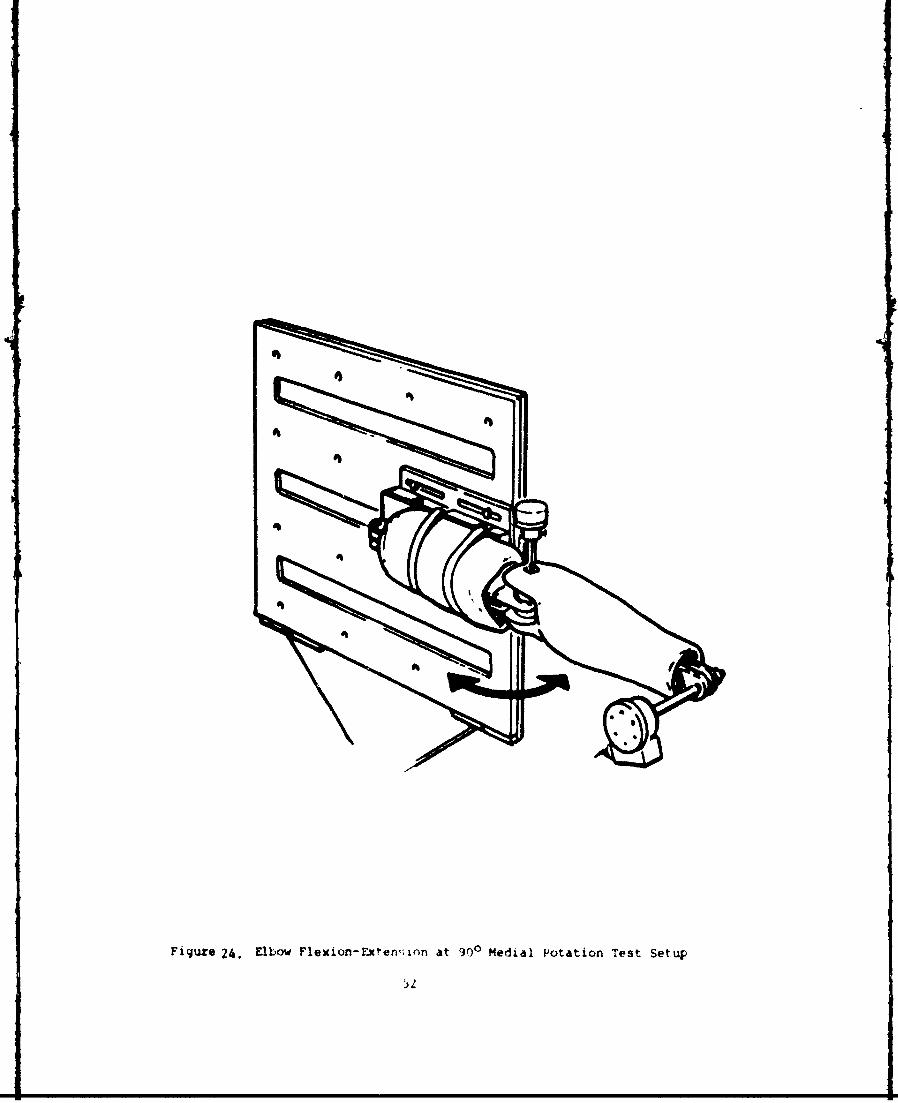
Figure 24. Elbow~ Flexion- Exten,; on at 900 M~edial Potation Test Setup
9S.4;lb Is
ISART,
liTtuisoN RIGHT ELBOWJ
94 lb in
LEFT ELBOJW
FIGURE 25. ELBOW FLEXION-EXTENSION AT 0' ROTATION FOR STANDING MANIKIN
I I Mu
7-7
RIGHT ELBOW
LEFT ELBOW
FIGURE i. ELBOW FLEXION-EXTENSION AT 90* MEDIAL ROTATION FORSTANOING MANIKIN
INOO
, _
RIGHT ELBOW
FLEIJON
90.4 b,
Ia
II... ...... .IS 11? .' T ... ..
IX~ O~ f I
LEFT ELBOW
FIGURE 27. ELBOW kL-XION-tXTENSION (,T 180" MEDIAL ROTATION FORSTANDING MANIKIN
I I
ii
RIGHT ELBOW
9.4 lb In i
utvfr.:om LEFT ELBOW
FIGURE 28. ELBOW FLEXION-EXTENSION AT 2100 MEDIAL ROTATION FORSTANDING MANIKIN
ft -~.-...-- - --
- 4 1
RIEHT ELBOW
S ItI
I..
L E F
L O
FIG RE 29. EL OW LE IO- E SI ON AT ", O~ IO O E TE A I I
' t
RIGHT ELBOW El1i
I~o
tx mnwl WM.Glb t.
I Is rLIN vI
LEFT ELBOW
FIGURE 'jO, ELBOW FLEXIOrN-EATENSION AT 90" MEDIAL ROTATION FOR
SEATED MANIKIN
I I
RIGHT ELBOW
E I
I[wl
Io n
9e 4 lb
_ I
1*
I 4 - -
.+ .. .4 .- '--- - c
RI H
TLBr
LEFT ELaOW
FIGURE 31. ELBOW FLEXION-EXTENSION AT 180 MEDIAL ROTATION FORSEATED ANIKN
59
°" II _ _
: i 1
LEFT ELBOW,
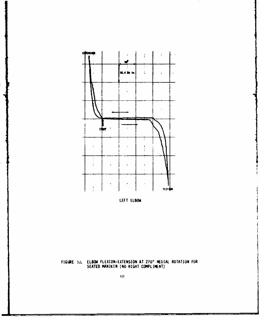
FIGURE 32. ELBOW FLEXION-EXTENSION AT 2700 MEDIAL ROTATION FORSEATED M4ANIKIN (NO RIGHT COMPLIMENT)
6--0
range of motion values were al so greater for the seated manikin
indicating a structural difference betweer the two manikins. The
extension bard stops were not as obvious as those found in the 00 and
lao0 medial rotation flexion-extension tests due to increased soft
covering interactions.
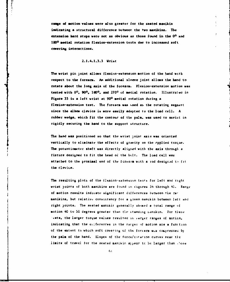
2.1.4.1.3.3 Wrist
The wrist pin joint allows flexion-extension motion of the hand eiitb
respect to the forearm. An additional sleeve joint allows the hand to
rotate about the long axis of the forearm. Flexion-extension notion was
tested with 00. 900, 1000. and 2700 of medial rotation. lllustrs'qva in
Figure 33 is a left wrist at 900 medial rotation during a
flexion-extension test. The forearm was used as tbe rotating segzet
since the elbow clevice is more easily adapted to the load cell. A
rubber wedge, wbich fit the contour of the pals. was used to assist in
rigidly securing the band to the support structure.
The hand was positioned so that the wrist joint axis was oriertedtvertically to eliminate tbe effects of gravity on the rpplied torrue.The potentiometer shaft was directly alibied with the axis through a
fixture designed to fit the head oi the bolt. The load cell was
attached to the proximal end of the fortarm with a rod desigr.ad to fit
the clevice.
The resulting plots of the f Aezion-extension testb for left and right
$ wrist joints of both manikins are found ir, t'igures 34 through 41. Rang
of noticn results indxi.ete significant differences betveen thse tv,
manikins, but relative consistency tot a iven manikin between left aniJ
right joints. The seated manikir generally sh,.bed a total range tf
notion 40 to 50 degrees greater then tlhe itanditg L.dnxkLn. For tg'e~t-
vats. the larger torque values resulted i i= aer~y ranges of motion.
indicating that the u):ferences in the raigeit )f motion are a fun(tion
of the extent to which soft coveri:.g 0i thc forisum ws co&presse; by
the pals of the hand. Slopes of the force/ ,,oation curvev near tie
limits of travel for the seated mankir. aj..ear tc P larger than ,iote
fi
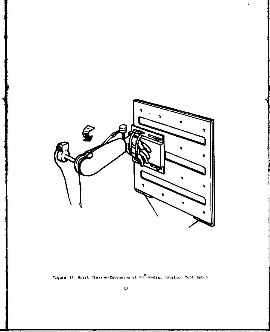
Figure 3.Wrist Flexion-Extension at 900Medial Rotation Test Setup
62
IM l,,t
* I kci
I 1
IS.lb,
o3V
4£4 i lb
ST F1Y
-I
LEFT WRIST
FIGURE 34. WRIST FLEXION-EXTENSIUN AT 0° ROTATION FOR STANDING MANIKIN
." •~W I' "i ,,,
RIGHT WRIST
r /bTJ~
I...............
64
RIGHT WRISTITEJUSION
46 4 lb
FiLlK LEFT WRIST
FIGURE 36. WRIST FLEXION-EXTENSION AT 180* MEDIAL ROTATION FORSTANDING MANIKIN
S,
- ERIGHT WRIST
i":
iSJ1.4 Iht Is - -
SWT
- -- -i~ ---
LEFT WRIST EitEwtO
FIGURE . wRIST FLEXION-EXTENSION AT 27UO MEDIAL ROTATION FOR
STANDING MANIKIN
If66
*~ l S'b ill
RIGHT WRIST
Rat
LEFT WRIST
FIGURE 38. WRIST FLEXION-EXTENSION AT U" ROTATION FOR SEATED MANIKIN
RIGHTI WRISFFIL
RIGHT WRIST
FICUE 3. WISTFLEION-XTESIO AT9-l MEDAL OTTIN.O
SETE 0AII
I~ L
RIGHT WRIST
LEFT WRIST
FIGURE 40. WRIST FLEX ION-EXTENSI ON AT 180'3 MEDIAL ROTATION FORSEATED MANIKIN
69
Ii~Ii
FGIU. i-E I AT
SEATED MANIKIN.
7 0
Liit Z'1 itLEFHT WRST
FIGUE '. WRST LEAIN-ETENION T 2OU MDIA ROTTIO FO
SETE MANKI
- Im dk4~bhl -,I* '- l7-
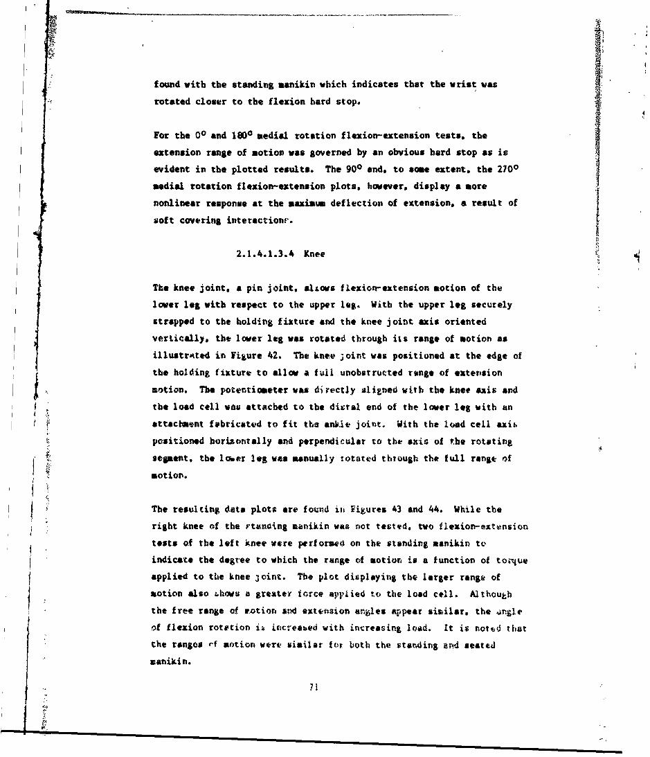
found with the standing manikin which indicates that the wrist was
rotated closer to the flexion hard stop.
For the 00 and 180o medial rotation flexion-extension tests, the
extension range of motion was governed by an obvious hard stop as is
evident in the plotted results. The 900 and, to some extent, the 2700
medial rotation flexion-extension plots, however, display a more
nonlinear response at the maximum deflection of extension, a result of
soft covering interactionr.
2.1.4.1.3.4 Knee
The knee joint, a pin joint, alLows flexion-extension notion of the
lower leg with respect to the upper leg. With the upper leg securely
strapped to the holding fixture and the knee joint axis oriented
vertically, the lower leg was rotated through its range of motion as
illustrated in Figure 42. The knee joint was positioned at the edge of
the holding fixture to allow a full unobstructed range of extension
Amotion. The potentiometer vs directly aligned with the knee axis andthe load cell wan attached to the diztal end of the lower leg with an
attachment fabricated to fit the ankie joint. With the load cell axis
positioned horizontally and perpendicular to the axis of the rotating
sepent, the lmer leg was manually :otated through the full range of
motion.
The resulting data plots are found it, Figures 43 and 44. While the
right knee of the rtanding manikin was not tented, two flexion-extension
tests of the left knee were performed on the standing asnikin tw,
indicate the degree to which the range of aotiot is a function of torque
applied to the knee joint. The plot displaying the larger range of
motion also Uhows a greater force apliied to the load cell. Al outh
the free range of u.otiort and extension angles appear similar, the ar-gle
of flexion rotetion iu iccreabed with increasing load. It is noted that
the rangos rf motion were similar fox both the starding or.d seated
manikin.
71
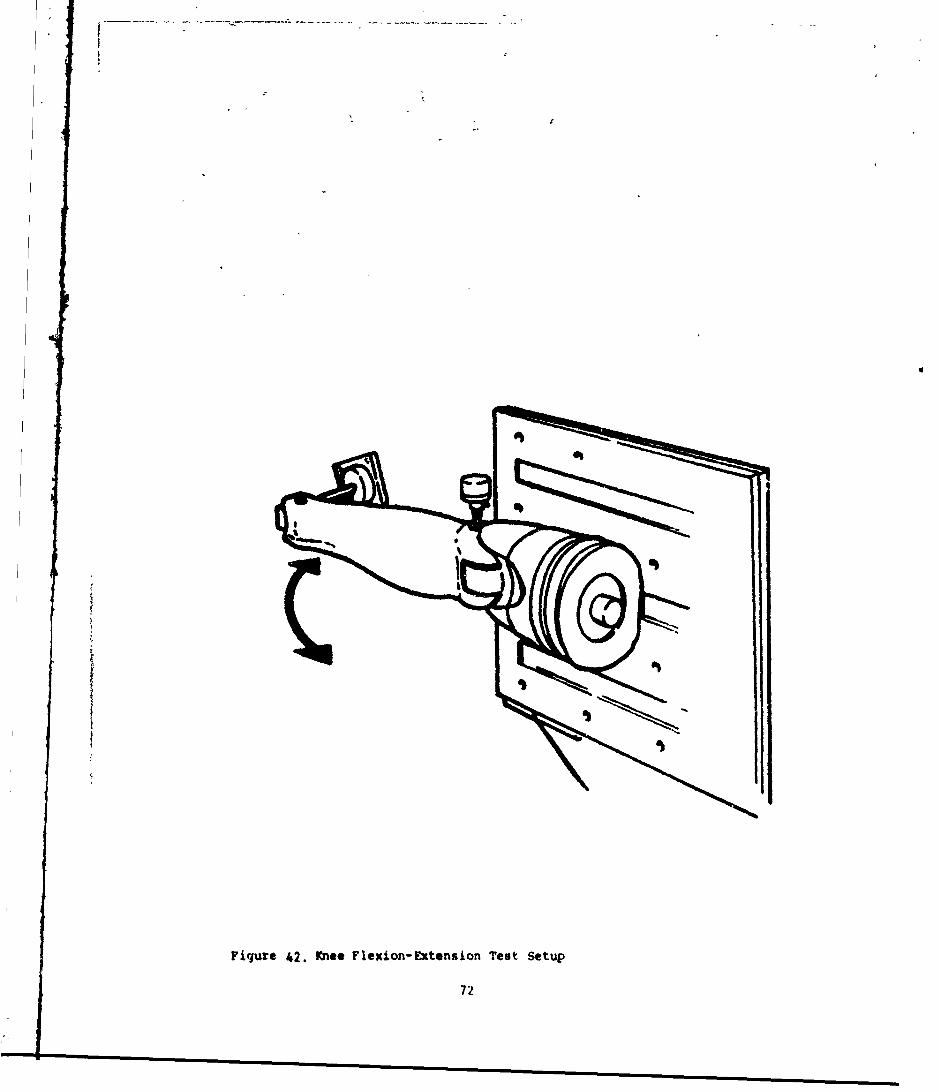
Figure 42. Kn** Flexion- Extension Test Setup
72
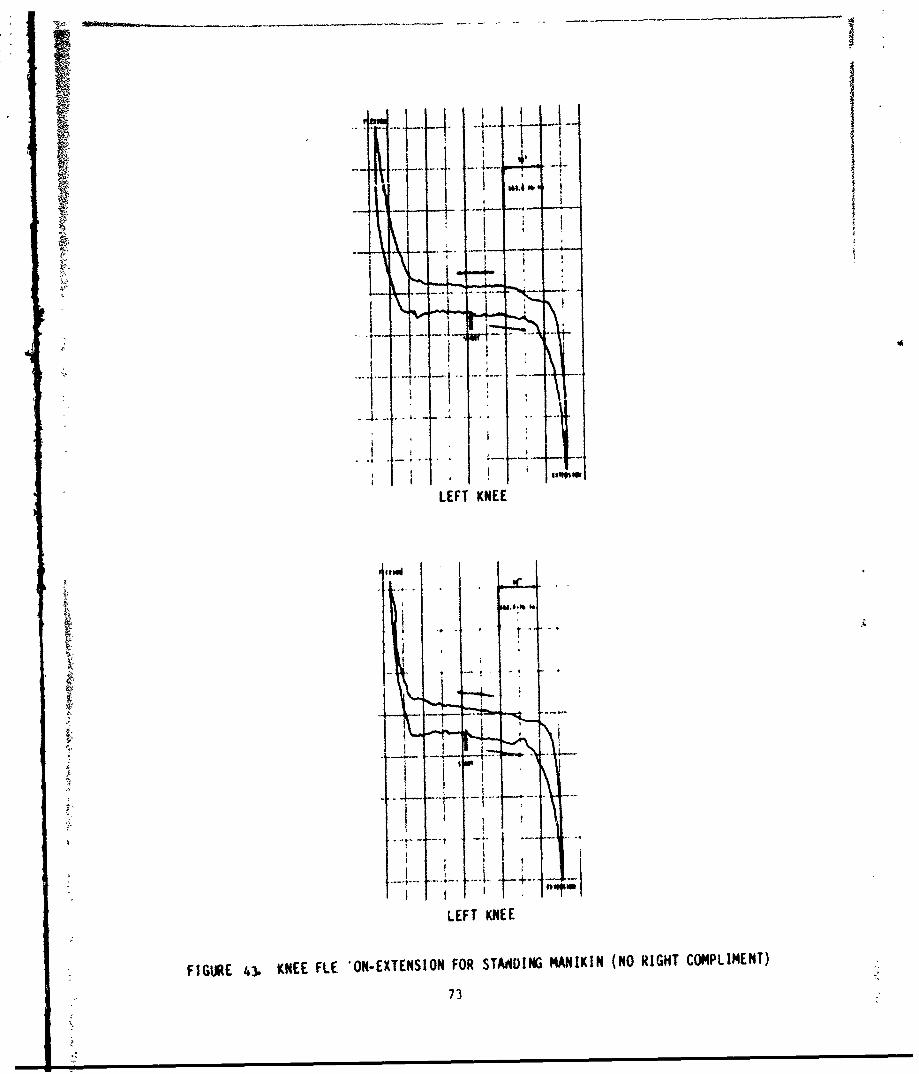
LEFT KNEE
FIGURE 43. KNEE FLE 'ON-EXTENSION FOR STMAD!NG MA4NIKIN (NO RIGHT COMPLIMENT)
73
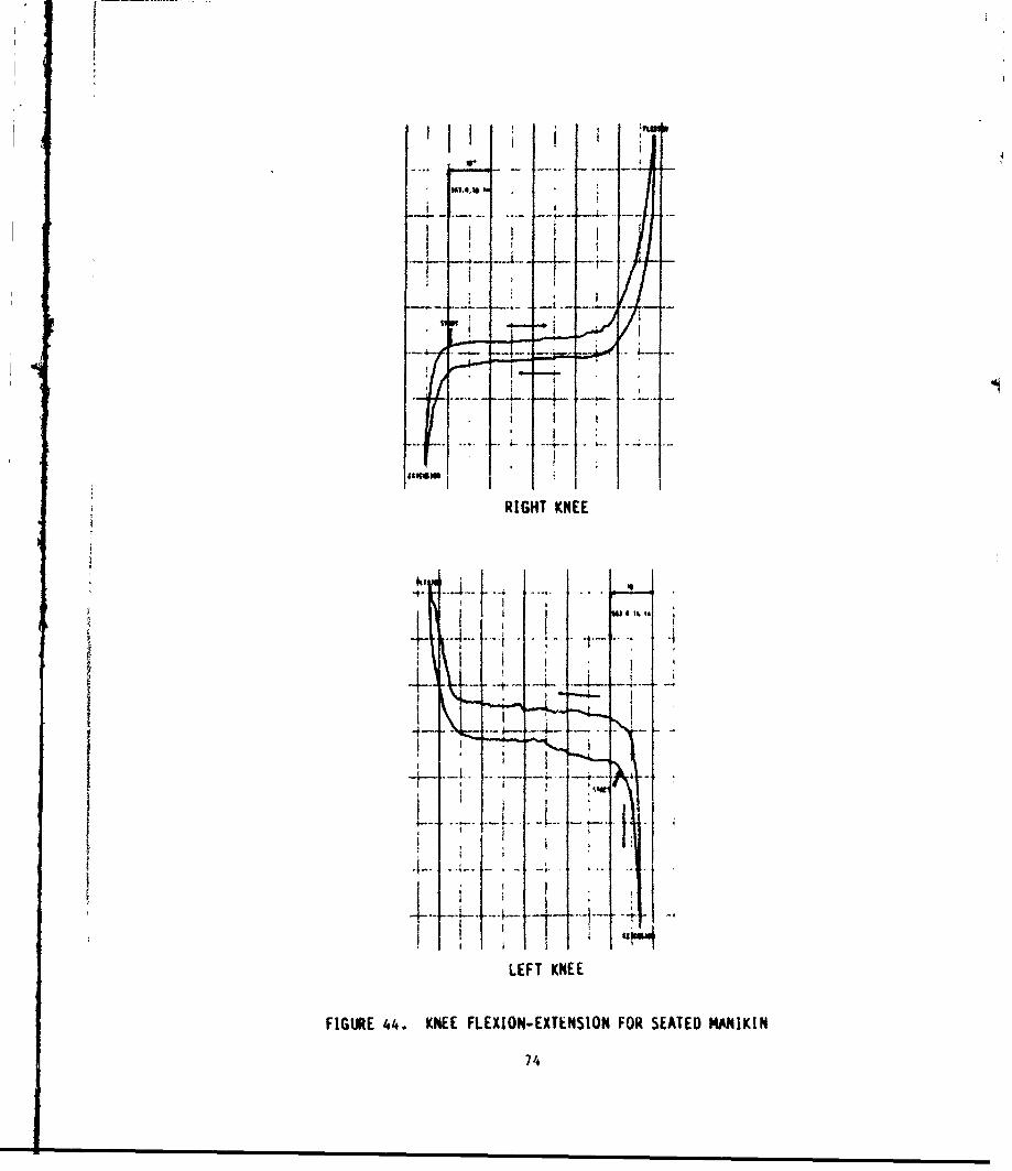
..-..... ..... ~ ~ -
RIGHT KNEE
IN
LEFT KNEE
FIGURE 44. KNEE FLEXION-EXTENSION FOR SEATED MANIKIN
7,4
2.1.4.1.3.5 Ankle
The ankle pin joint allows plantar flexion and dorsiflexion of the foot
with respect to the lower leg. The lower leg was used as the rotating
segment and the foot was securely claped to the holding fixture.
orienting the joint axis vertically. See Figure 45. The potentiometer
shaft was aligned with the ankle bolt and the load cell was attached to
the proximal end of the lower leg. the rotating segment, and was
positioned horizontally and perpendicular to the long bone axis. Both
left and right ankle joints were tested on each manikin.
The resulting joint resistance versus angle of rotation plots are
presented in Figures 46 and 47. Range of motion values indicate
consistency between left and right joints on each manikin, but a 15 to
30 degree larger range of notion for the seated manikin. These
differences do not appear to be a function of torque, but are due to
structural differences betweetr the manikins. For all of the resu2ting
ankle curves, the stops which govern both flexion and extension appear
to be due to hard mechanical stops.
2.1.4.1.3.6 Hip
The hip joint, which i- a ball and socket joint. allows moves ?nt in the
flexion-extension. abduction-adduction. and rotational directions. For
thib joint, the resistance of the ball to move within the ball and
socket joint is determined by the tightnec of cap screws holding the
covering plate. For a joint loosely torqued. however. resistance is
primarily provided by skin to skin interactions and hard stops. The
seated pelvis is molded such that the upper leg is in a 90 degree
flexion orientation. The standing pelvis is molded to allow free
rotation in the flexion-extension and abduction-adduction directions.
The flexion-extension dnd abduction-adduction teuts were performed at a
90 degree fVexion starting position for the seted manikin and in the
anatomical standing starting position for the standing manikin.
75
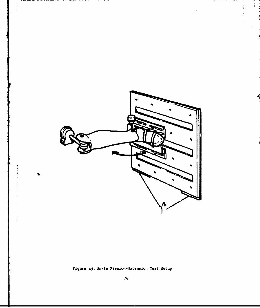
U.k
FiquVO 45. Anki. Flexion-Extonsio" Test Setup
76
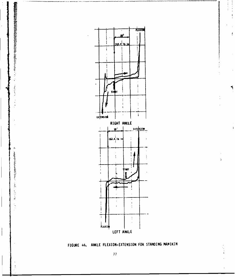
RIGHT ANKLE
30' Exit SION
LEFT ANKLE
FIGURE 46. ANKLE FLEXION-EXTENSION FOR STANDING MANIKIN
77
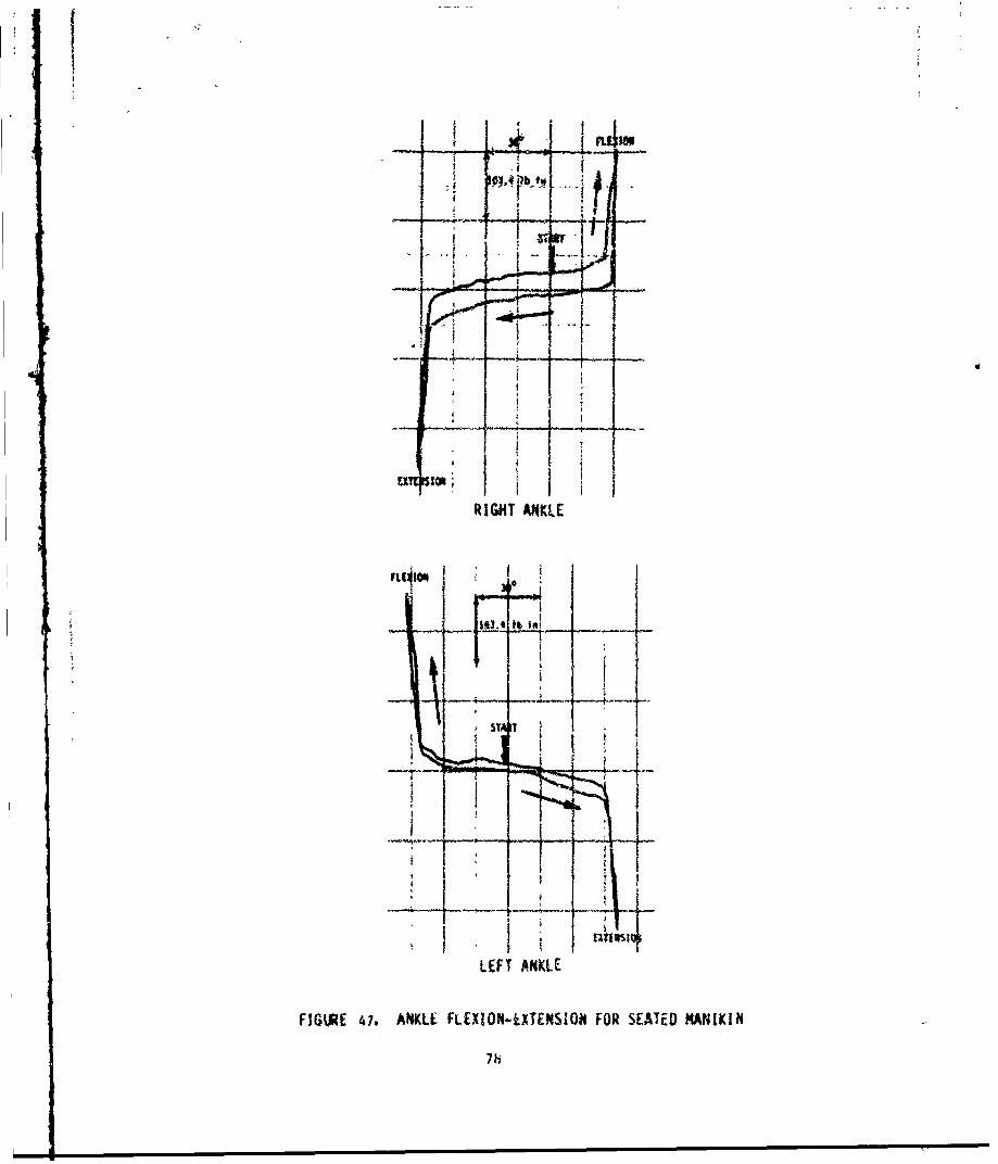
If
sI I ~ ~~ IA
RIGHT ANKLE
V liAI
11
LEFT ANKLE
FIGURE V7. ANKLE FLEXION-IXTERSION FOR SEATED MANIKIN
7h
Since the ball and socket joint is centered within the molded pelvis. the
pot used to measure the rotation angle was centered over the joint and
was manually rotated to follow the joint rotation. For
abduction-adduction tests, the seated and standing pelvis were
positioned upright, supported, and secured as shown in Figure 48. The
load cell axis was positioned horizontally and perpendicular to the
upper leg long bone axis and was used to manually rotate the leg through
the range of motion.
For the flexion-extension tests, the pelvis was positioned on its side
to orient the joint axis vertically as shown in Figure 49. The
potentiometer axis was again held above the joint and positioned
coaxially with the axis of rotation. The pot was rotased manually to
follow the rotation of the upper leg. The load cell axis was positioned
horizontally and perpendicular to the upper leg long axis and the load
cell wos used to manually rotate the upper leg through the range of
motion. Flexion-extension and abduction-adduction tests were conducted
on the left and right joints for both manikins.
Joint torque versus angle of rotation results are presented in Figures
50 through 53. Range of motion values from the seated manikin are as
such as 126 degrees smaller than the standing manikin. These
differences are an obvious result of mechavical structure differences
and the skin to skin interaction of the seated pelvis. The seated
polvis has an extended hip flesh which surrounds the uppermost part of
the upper leg and. thus. greatly restricts the range of motion for both
flexion-extension and abduction-adduction movement. The curves dispioy
no tree range of motion fo'r the seated manikin. The standing manikin.
however, is not restricted and allows a limited amount of free range of
motion before reaching soft coverinU interference.
79
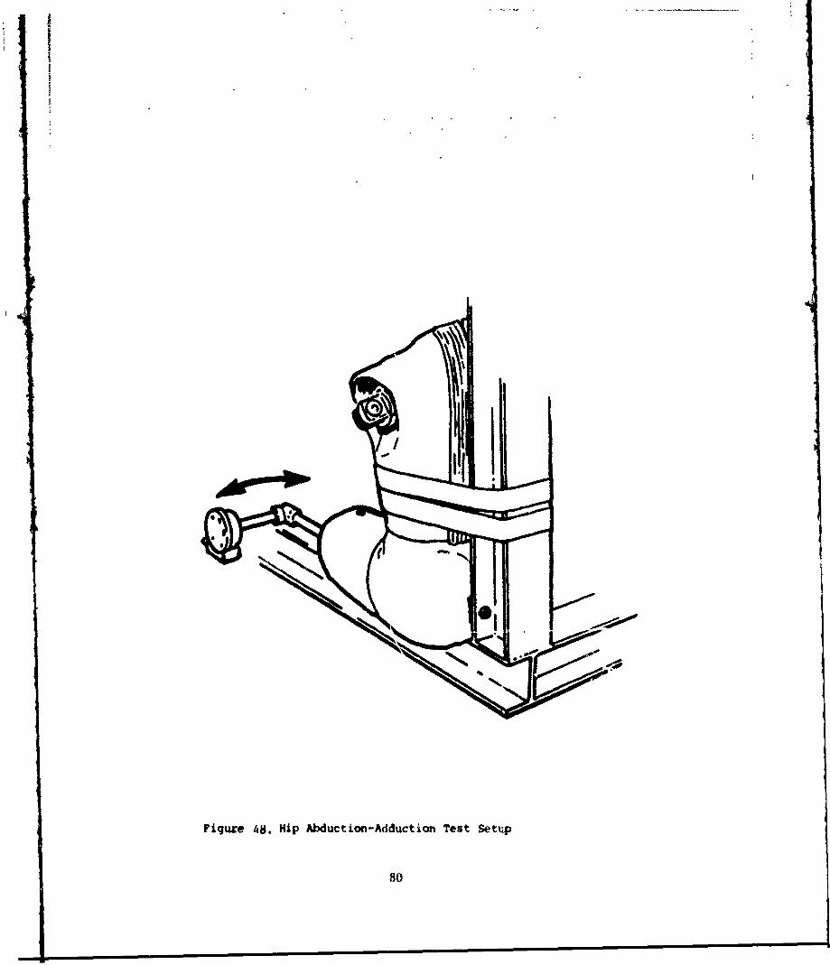
101
Figu~re 4S. Hip Abduct ion-Adduct ion Test Setup
80)
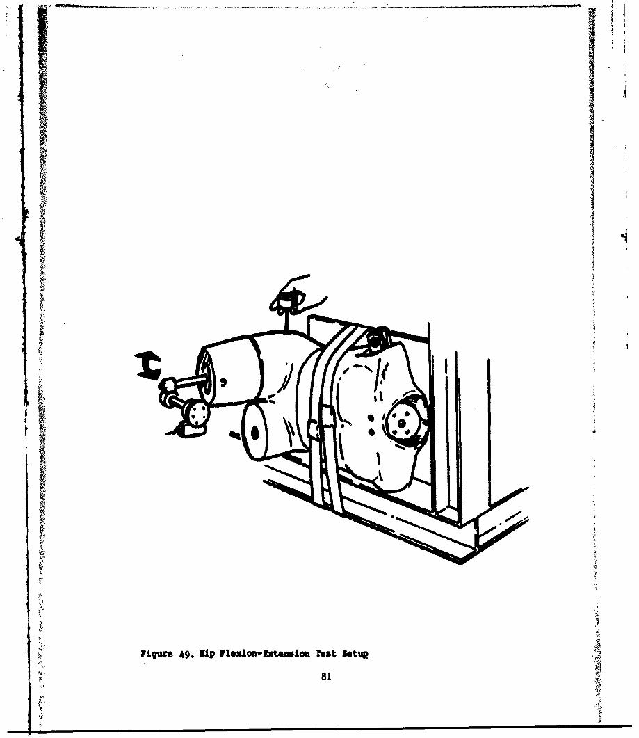
811
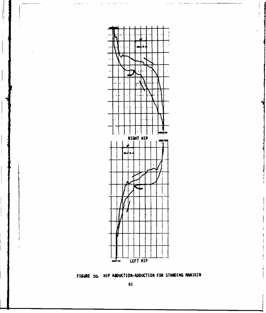
ki
stoo
- .-- : -N
RIGHT HIP
II
I I
LEFT HIP
FIGURE 50. HIP ABWUCTION-ADOUCTION FOR STANDING MANIKIN
82
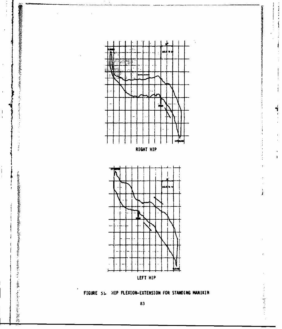
iI 1A I i
RIGHT HIP
LII f- - I- A
I- t§ 7 'k
LEFT HIP
FIGURE 51. H1IP FLEXION-EXTENSION FOR STANDING MANIKIN
83
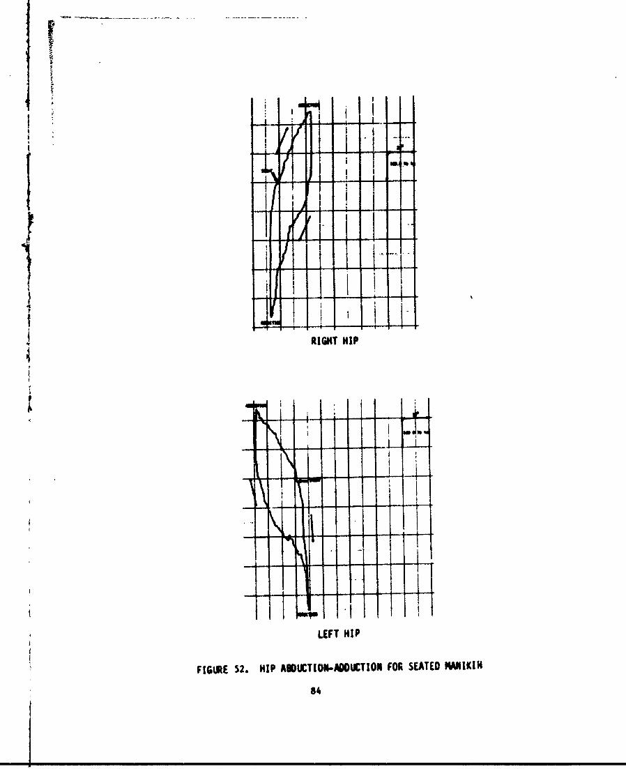
II i1
4 I
- I-l
....I_.. - _.- __
II
i RIGHT HIP
4r
I ,
I I, ii..
•1 -
* LEFT HIP
FIGURE $2. HIP AIDUCTIOK-AMOUCTION! FOR SEATED MANIIKIN
84
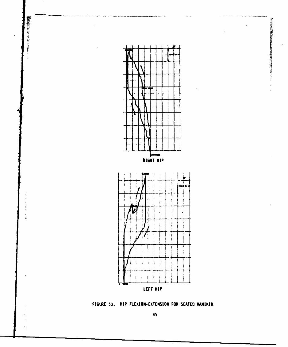
1~- I
- *1
~-I
RIGHT HIP
K; .1
-. _ j- I- __ _
LEFT HIP
FIGURE 53. HIP FLEXIOK-EXTENSION FOR SEATED MANIKIN
85
2.1.4.2 Determination of Joint lange of notion
he rang* of motion of a joint is detemined by hard stop@. soft stops.
and soft covering itreractions. The bard stops provide definite notion
ilmitatio s of a joint, while the soft stops or soft covering
interactions prevent free rafse of motion and produce resistance as 8
function of angle of rotation. In the latter cases a all defined range
of motion value cannot be determined as this value becomes a function of
force applied to the rotating segi et. The higher the torque applied.
the more the skin or soft stop defem end the greater the range of
motion. The slope of the force/deflection curve provides some
indication of how close to the full range of notion the joint has been
moved. As the slope approeches infinity, where no amount of applied
torque* increases the angle of rotation. the value of the rangse of
aotion at this point is the maximum. for most of tb experimental
curves developed, however, the maxim range possible vs. not reached.
The values for the Toge of notion differed between the left end right
joints for a single manikin and also from manikin to manikin. For
example, the joint characteristic curves o( wrist flexion-extension at
00 medial rotation joint tests for the standing end seated manikin.
shown in figures 34 and 38. show that the free range o, motion, that
range which experiences little or no resistance, is aproimately 300
greater for the right joint than was easured or, the left joint of the
standing manikin. Additionally, the values for extension beyond the
free range of notion are about 100 greater for the seated manikin than
the values measured for the standing manikin. The larger values for the
seated manikin suggest a structural difference between the two manikins.
2.1.4.3 Determination of the Characteristics of the Lumber
spine
The olded rubber lumber spine Ol 'ws flxion-extension and lateral
movament of the thorax with respect to the pelvis. Deflection
resistance of the spine is dependent upon the cheracteristics of the
natural rubber, the shape of the spire, and the strengtb of the steel
86
cable or cables. which are centered axially through the spine. The
seated manikin spine is curved to simulate the seated posture while the
standing manikin spine is a straight cylinder. Both spines were tested
Cto determine their respective, stiffnmess properties.
2.1.4.3.1 Spine of Standing Manikin
The straight spin* of the standing manikin was statically tested in
flexion. Since the spine is cylinderaally symtrice the bending
stiff nesses in flexion, etension. and lateral directions are the ame.
T wo tests woe peformed to evaluate the degree of repeatability in
determining the mmnt versus angle of deflection curve. These tests
vote conducted about an hour apart to allow a recovery period for the
rubber to release its stored energy from the previous test.
In the test setup the spine was positioned horizontally and the base of
the spine ws3 securely clamped to a holding from*. The top of tbe spine
was attached to a cable through which the load was applied. This test
setup is illustrated in figure 54. A load cell was attached to the
cable and the applied load was measured and plotted against the angular
rotationI of the tip of the spine. measured by an inclinometer. Section
22 -- >1. describes the method used to convert the measured force to
the applied somet at the base of tbe spine.
The results of the tests are presented in figure 55. Shown are plots of
applied moment versus angle of rotation. As can be seem from the plots.
the straight spine displayed a linear response with applied moment Over
the angle of rotation tested which results in a stiffness value of about
48 in-lb/deg for bending in all three directions. To further quantify
the spine stiffness, the spine should be deflected beyond 30 degrees.
Although the straigiat spine bad the ane bending stiff msses in all
directions. tho abdounl'. insert provides a stiffening effect in tbe
flexion and lateral directions when inserted in the" manikin. To
detemine this stiffening ef fact. the spine was sthtically tested with
87
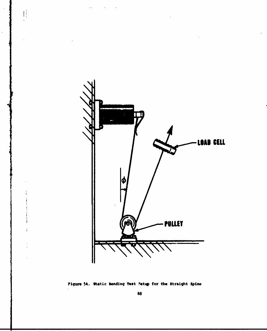
LUAU CELL
Figure 54. Static bending Test q5t~ for tbe Straight Spino
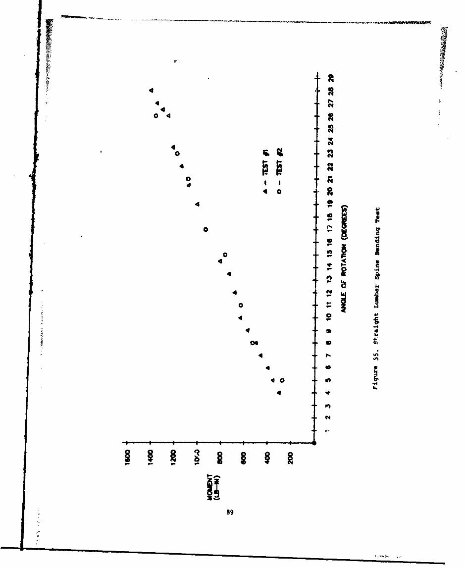
0~ -
40
4
04
0.4
44
00u4 4~
40
4
3, beJr
S 9f
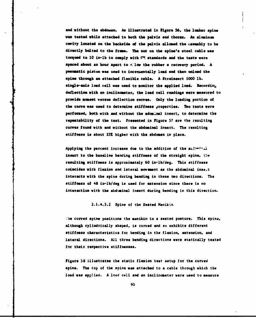
and without the abdoemn. As illustrated in Figure 56. the lumber spine
was tested while attached to both the pelvis and thorax. An aluminum
cavity located on the backside of the pelvis slloed the assembly to be
directly bolted to the frame. The nut on the spine's steel cable was
torqued to 10 in-lb to comply with (". standards and the tests were
spaced about an hour apart to o- o the rubber a recovery period. A
pneumatic piston was used to incewAentally load and than unload the
spine throueh an attached flexible cable. A Strainsert 1000 lb.
single-axis load cell was used to monitor the applied load. Racordin"
deflection with an inclinometer, the load cell readings were measured to
provide moment versus deflection curves. Only the loading portion of
the curve was used to determine stiffness properties. Two tests were
perfortd, both with and without the adomnl insert, to determine the
repeatability of the test. Presented in figure 57 are the resulting
curves found with and without the abdominal insert. The resulting
stiffness is about 23Z higher with the abdomen in place.
Applying the percent increase due to the addition of the sL -"'
insert to the baseline bending stiffness of the straight spine. .'e
resulting stiffness is approximately 60 in-lb/deS . This stiffness
coincides with flexion and lateral movement as the abdominal inse~t
interacts with the spine during bending in these two directions. The
stiffness of 48 in-lb/deg is used for extension since there is no
interaction with the abdjainal insert during bending in this direction.
2.1.4.3.2 Spine of the Seated Manikin
.le curved spine positions the manikin in a seated posture. This spine.
although cylindrically shaped, is curved and so exhibits different
stiffness characteristics for bending in the flexion. extension, and
lateral directions. All three bending directions were statically tested
for their repective stiftnesses.
figure 58 illustrates the static fleion test setup for the curved
spine. The top of the spine was attached to a cable through which the
load was applied. A loaO cell and an inclinometer were used to measure
90
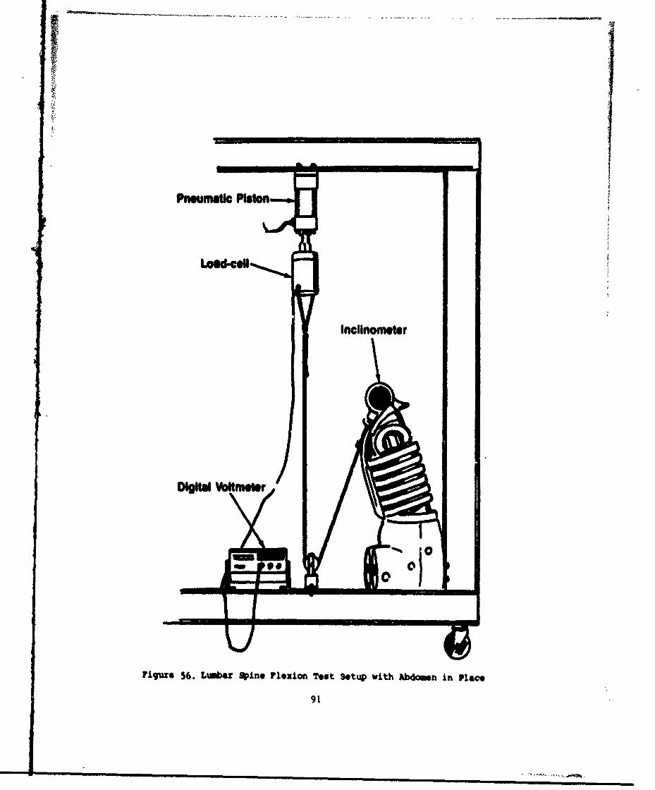
Inclinomtr
D ~W otm e0L M-
01
figuxe 56. LUinba R~dne Flexion Test Setup with Abdomen in Viece
91
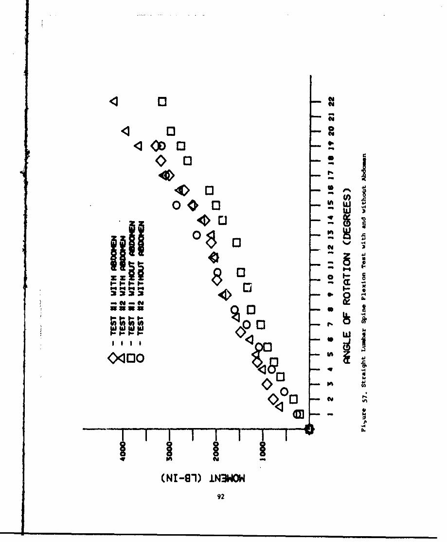
00I 0
cI~O0
0~00
NA04%0
3333
00
,, ..
(NI-W1) IN34OW
92
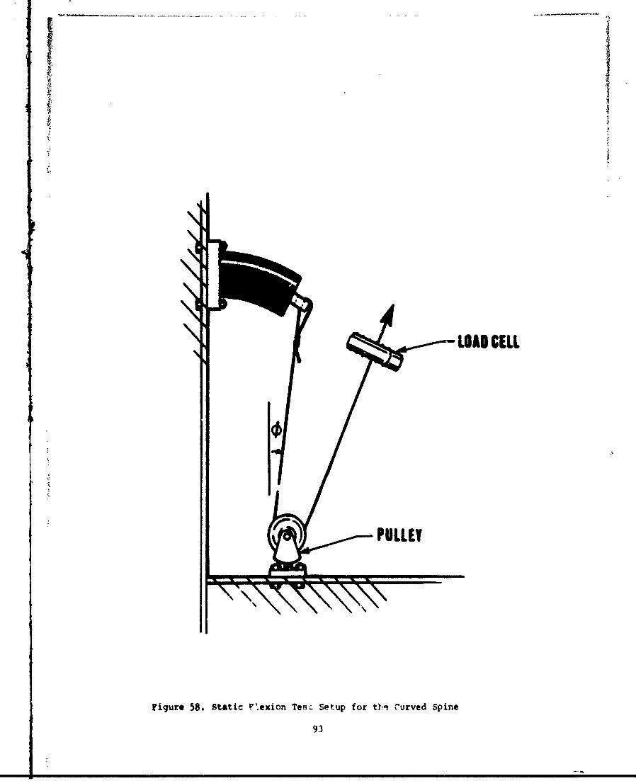
LOAD CELL
Figure 58. Static F exion Tesc Setup for thb Curved Spine
93
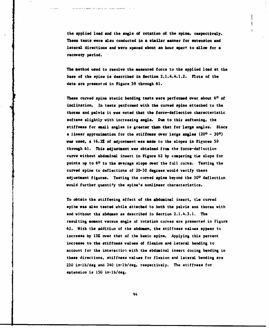
the applied load and the angle of rotation of the spine, respectively.
These testsa were also conducted in a similar manner for extension and
lateral directions and were spaced about an hour apart to allow for a
recovery period.
The method used to resolve the measured force to the applied load at the
base of the spin* is described in Section 2.1.4.4.1.2. Plots of the
data are present.d in figure 59 through 61.
These cutrved spine static bending tests were perf ormed over about 60 of
inclination. In tests performed with the curved spine attached to the
thorax and pelvis it was noted that the force-deflection characteristic
softens slightly with increasing angle. Due to this softening, the
stiffness for small angles is greater than that for large angles. Since
a linear approximation for the stiffness over large angles (200 - 300)
was used, a 16.22 of adjustment was made to the slopes in figures 59
through 61.* This adjustment was obtained from the force-deflection
curve without abdominal insert in figure 62 by comparing tbe slope for
points up to 60 to the average slope over the full cuirve. Testing the
curved spine to deflections of 20-30 degrees would verify these
adjustment figures. Testing the curved spine beyond the 300 deflection
would further quantify the spine's nonlinear characteristics.
To obtain the stiffening effect of the abdominal insert, teA curved
spine wos also tested while attached to both the pelvis and thorax with
and without the abdomen as described in Section 2.1.4.3.1. The
resulting moment versus angle of rotation cuives are presented in Figure
62. With the additiun of the abdomen, the stiffness values appear to
increase by 131 over that of the basic spine. Applying this percent
increase to the stiffness values of fleuion ard lateral bending to
account for the interoction with the abdominal insert during bending in
these directions, stiffness values f or flexion and lateral bending are
230 in-lb/deg and 340 in-lb/cleg. respectively. The stiffness for
extension is 150 in-lb/deg.
94

1 4 0 0 o
a 0
1 2 0 0 -0
aAO0S1
0 0 0 - -
800 -- A
MOMENT(LB-IN)
0600
400 A-TEST #1
0-- EST #2
200 -
1 2 3 4 5 6
ANGLE OF ROTAnON (DEGREES)
Figure 59. Curvea Lumbar Spine Flexion Test
95
1800 -
1400 0OA
A1200 0 0
MOMENT 1000(LB-IN) o
A
0
400 A - TEST #1
0 - TEST #20
200
I- I - I 1 2 3 4 5 6 7 8
ANGLE OF ROTATION (DEGREES)
Fiqure 60. Curved Lwbr Spine utenvion Test
96
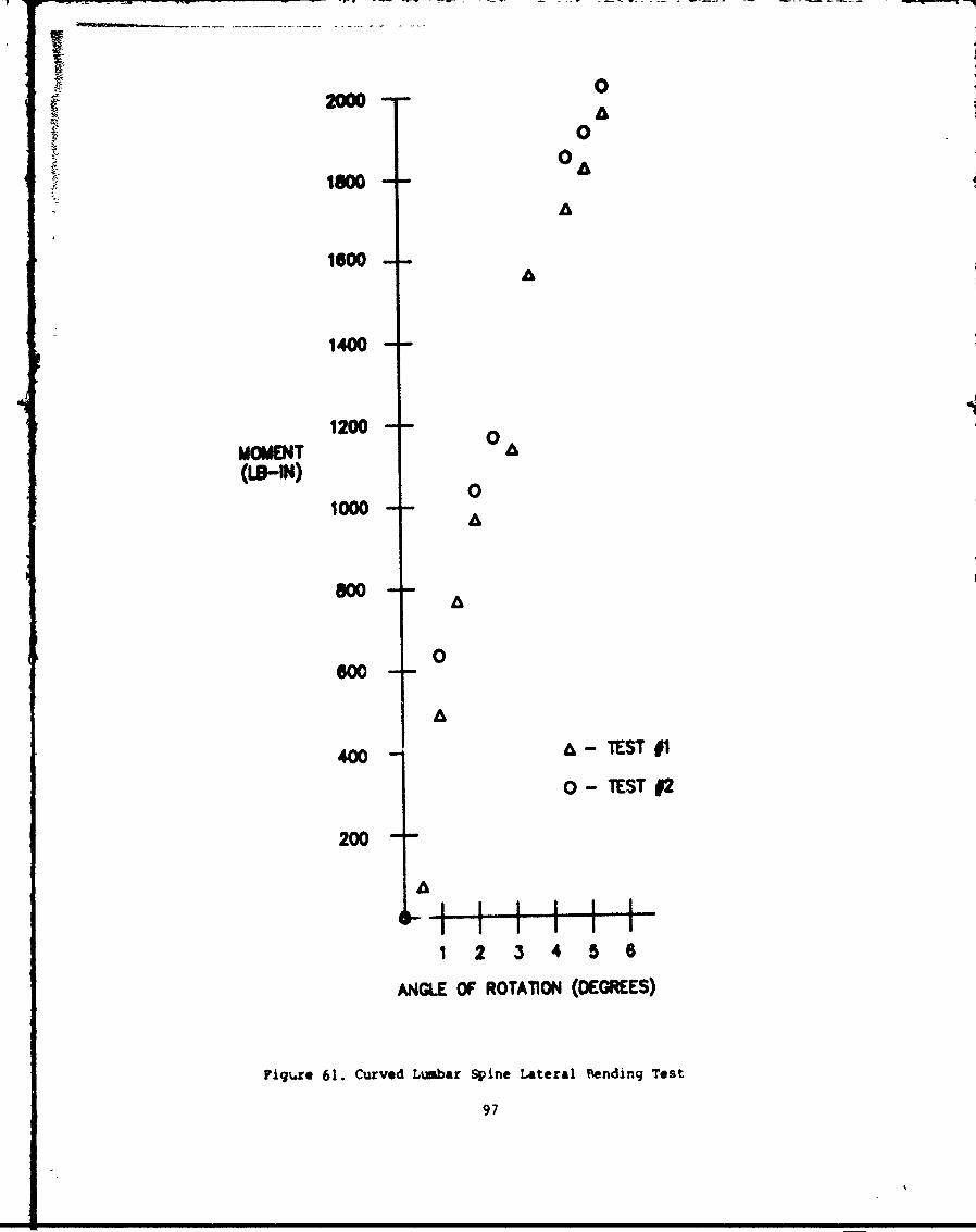
02000i oA
00 A
low
A
1600A
1400
1200 0MOMENT A(LB-IN) 0
1000 A
600 A
0
600
A
400 A- EST I1
0- TEST 92
200
A
Ii ! I I1 2 3 4 5 6
ANGLE OF ROTATION (DEGREES)
Figtre 61. Curved Lumbar Spine Lateral Pending Test
97
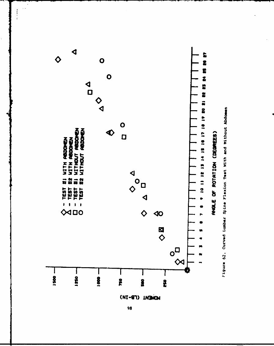
4 0
03
0 0
0 0
44J
74
ama
98
2.1.4.4 betendmetiom of the Characteristics of theNybrid 3111 Hecl
The Nrybid 11I mach allows twrieml. fleziom, extension. an lateral
noti.. of the head with respect to the thora. Mhe neck is constructed
of alumiam plates. repremeatiag vertebral elements. bonded togetherwith alterate sections of butyl elastamer. the axial stremgtb of the
neck is embaced by a steel cable which is blted thremgb the center ofthe mack. Saw cuts througha the anterior side of the neck provide
reduced ev'emsiom bending tesistmce, without affecting f lexion. Static
and dynamic tests were performed on the necks od the standing anod seated
manikin.; to detemine their stiffness characteristics
2.1.4.4.1 Static Tests
2.1.4.4.1.1 Test Procedure
In order to conduct tests of the neck to determine the bending
stiffnesses in the flexion. extension. and lateral directions, the neck
was loaded to obtain a moment versus anglt of deflection curve in the&mne manner as the tests of the lumbar spine. With the base of the neck
rigidly secured to the holding frame in a horizontal plain. the top of
the neck was attached to a cable through which the load was applied.
figure 63 illustrates the test setup for the static neck test. A load
cell was attached to the loading cable to measure the applied load and
the angular rotation of the element was measured with an inclinometer.
The method described in Section 2.1.4.4.1.2 was used to convert the
measured force to the applied moment at the base of the neck. Two tests
were performed for each configuration of both necks allowing an hour in
between tests for a recovery period.
2.1.4.4.1.2 D)ata Reduction Procedures and Results
The data reduction procedure outlined herein was that used to reduce the
test data obtained for the lumbar siines as well as the neck since all
teots were conducted usint the est test &etup and procedure.
99
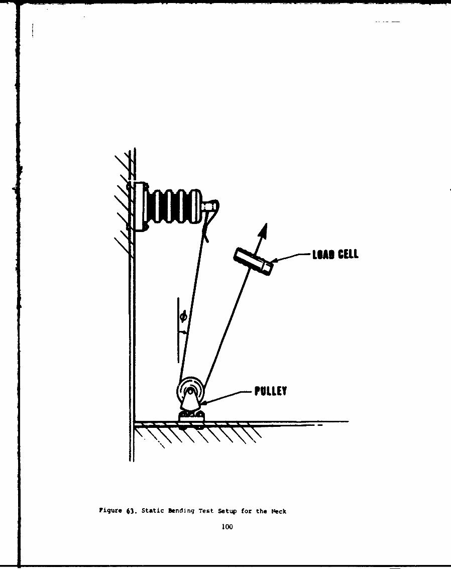
LSUI CELL
Figure 63. Static Sending Test Setup for the P'eck
100
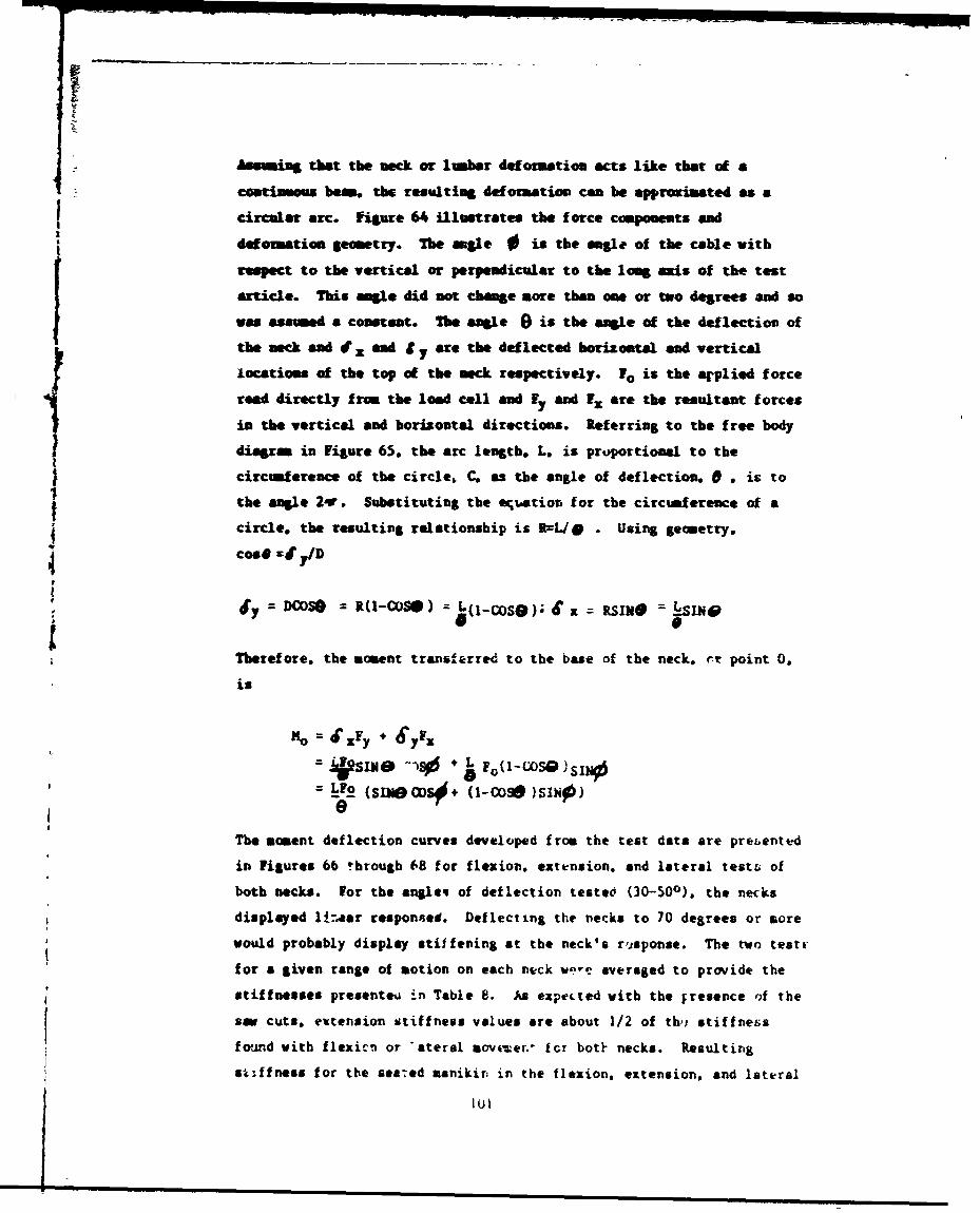
T
Auming that the neck or lumber defosatio acts like that of a
coatimous beso6 the resulting deformation can be approximated as a
circular arc. Figure 64 illustrates the force components and
defomation geometry. The angle 0 is the angle of the cable with
respect to the vertical or perpendicular to the long axis of the test
article. This mogle did not change more than one or two degrees and so
was easmed a constant. The angle (e is the angle of the deflection of
the neck and it x and a y are the deflected borizontal and vertical
locatios of the top of the neck respectively. F. is the arplied forceread directly f rm the load call and Fy and Ex are the resultant f orces
in the vertical and horizontal directions. Referring to the free body
diagram in Figure 65. the arc length, L. is proportional to the
circumference of the circle, C, as the angle of deflection, 0 , is to
the angle 24r. Substituting the equation for the circumference of a
circle, the resulting relationship is RrL/* . Using geometry.
cos@ =1r y/D
tS4"y = D~COSO = RO-COSO ) = L(I-CosO); If x = RI@ = SV
*Therefore. the moment transferred to the base of the neck. rr point 0.
is
No= 4F y & yFx
=45N L~ 'kW DS +O-CO Q)SINJO
The moment deflection curves developed from the test data are preLented
in Figures 6b through 68 for flexion. extension, and lateral testG of
both necks. for the angleq of deflection tested (30-500). the necks
displayed li.aar reaponseE. Deflecting the necks to 70 degrees or more
would probably display stiffening at the neck's risponse. The two testv
for a given range of motion on each neck ws-ve averaged to provide the
stiffnesses presentea in Table 8. As expected with the ;resence of the
am cuts. extension stiffness values are about 1/2 of th, stiffnessfound with flexicn or ateral soviwer., for bot necks. Resulting
st..ffness for the sea:ed manikin in the flexion, extension, and lateral
Siti
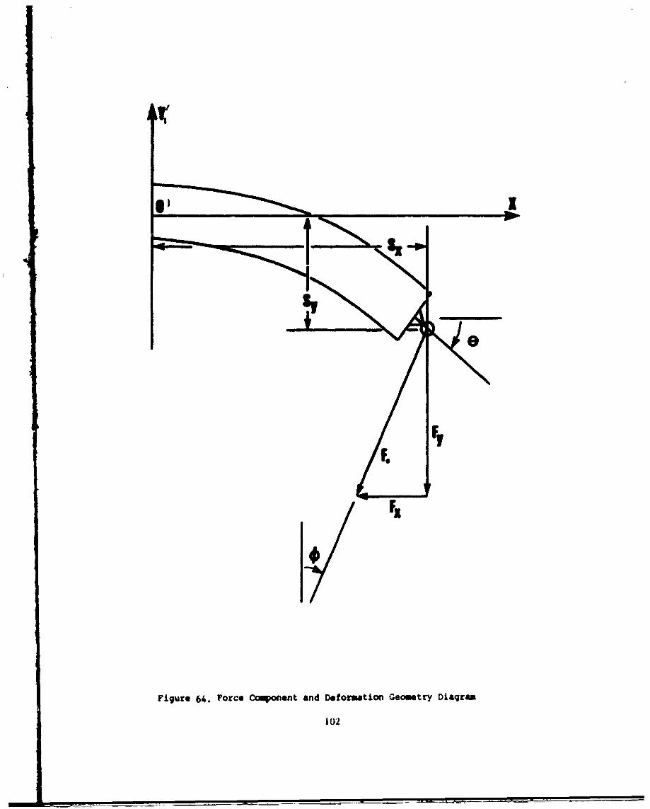
Fiqur* 64. Force COqoMn~nt and Deformation Geometry Diagram
102
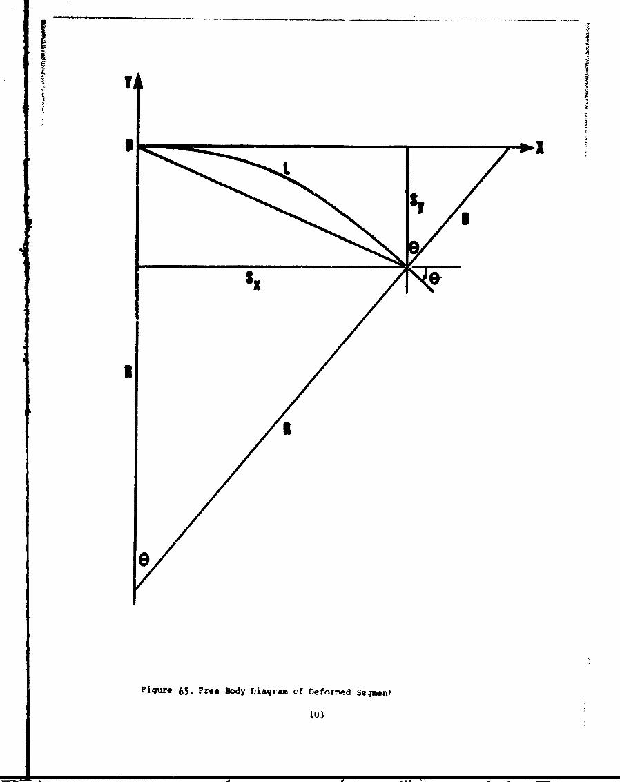
103
@0 C4
4. ad
lii C1
000 a
C41C
C4 .
00
+ 44w
4.00 0
4.
+00
44 w
4)
400
C44
194
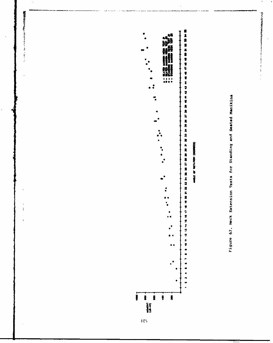
Ia
* 3*4Is~.
*
a g333 5
3* lIEU I4* liii I* sail
* Ia I
400* 3S
.4I
a a0
* '"4
a "-I
4 a zU.U, V
0* aa 4
4 30
.4 VC
9 3 4
1 0'a 5
* 354
0 4 cn
b 0* 4*
44,
* 130 C
0.4 a ".4U,* C* 4,
'a4%
94 * 14 9
6
~0
4,
.40'
06**
9*
* 0
9
U,9
U.
'II''
I;I C~
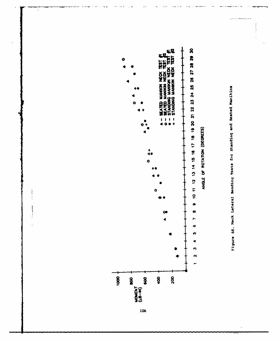
0 0 ( - '4
4 *1
00~~ o'
0+ 00
*
C44
40
0 U9
000
406
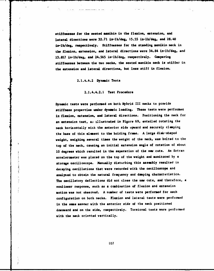
stiffnesses for the seated manikin in the flexion, extension, and
lateral directions were 32.71 in-lb/deg. 15.55 in-lb/deg. and 28.40
in-lb/deg, respectively. Stiffnesses for the standing manikin neck in
the flexion, extension. and lateral directions were 34.84 in-lb/deg. and
13.817 in-lb/deg. and 24.565 in-lb/deg. respectively. Comparing
stiffnesses between the two necks, the seated manikin neck is stiffer in
the extension and lateral directions, but less stiff in flexion.
2.1.4.4.2 Dynamic Tests
2.1.4.4.2.1 Test Procedure
Dynamic tests were performed on both Hybrid III necks to provide
stiffness properties under dynamic loading. These tests were performea
in flexion. extension, and lateral directions. Positioning the neck for
an extensicn test. *4 illustrated in Figure 69. entailed rotating the
neck horizontally with the anterior side upward and securely clamping
the base of this element to the holding frame. A large disk-shaped
weight, weighing several times the weight of the neck, was bolted to the
top of the neck, causing an initial extension angle of rotation of about
10 degrees which resulted in the separation of the saw cuts. An Entran
accelerometer was placed on the top of the weight and monitored by a
storage oscilloscope. Manually disturbing this assembly resulted in
decaying oscillations that were recorded with the oscilloscope and
analysed to obtain the natural frequency and damping characteristics.
The oscillatory deflections did not close the saw cuts, and therefore, a
nonlinear response, such as a combination of flexion and extension
motion was not observed. A number of tests were performed for each
configuration on both necks. Flexion and lateral tests were performed
in the same manner with the anterior side of the neck positioned
downward and on the sides respectively. Torsional tests were performed
with the neck oriented vertically.
107
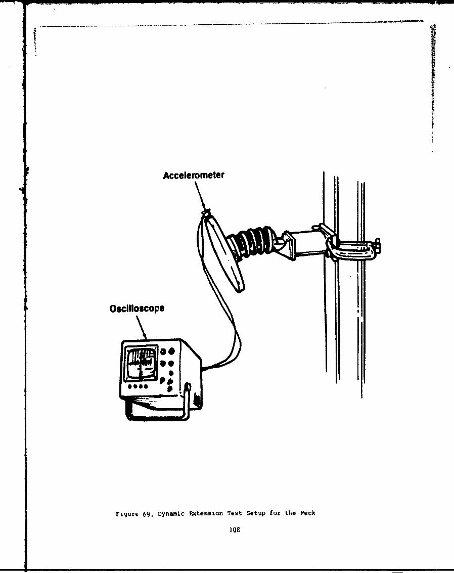
Accelerometer
Oscilloscope
Figure 69. Dynbamic Fbtensiozi Test Setup for the P~eck
108
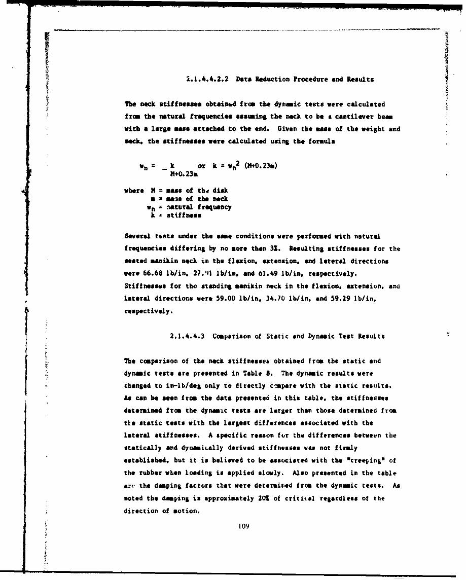
I.2.1.4.4.2.2 Data Reduction Procedure and Results
xThe neck stiffnesses obtained from the dynamic tests were calculated
from the natural frequencies assuing the neck to be a cantilever beam
with a large ass attached to the end. Given the mass of the weight and
neck, the stiffnesses were calculated using the foruula
" k or k = wn2 (4+0.23m)M-0. 23&
where N = mass of tb- diska = ma3s of the neck
Vn = natural frequencyk r stiffness
Several tests under the same conditions were performed with natural
frequencies differing by no more than 31. Resulting stiffnesses for the
seated manikin neck in the flexion, extension, and lateral directions
were 66.68 lb/in. 27.111 lb/in. and 61.49 lb/in, respectively.
Stiffnesses for the standing manikin neck in the flexion, extension, and
lateral directions were 59.00 lb/in. 34.70 lb/in. and 59.29 lb/in.respectively.
2.1.4.4.3 Comparison of Static end Dynamic Test Results
The comparison of the neck stiffnesses obtained from the static and
dynamic tests are presented in Table 8. The dynamic results were
changed to in-lb/des only to directly c-2pare with the static results.
As can be seen from the data presented in this table, the stiffnesses
determined from the dynamic tests are larger than those determined from
tke static tests with the largest differences associated with the
lateral stiffnesses. A specific reason for the differences between the
statically and dynamically derived stiffnesseu was not firmly
established, but it is believed to be associated with the *creeping" of
the rubber when loading is applied slowly. Also presented in the table
art, the damping factors that were determined from the dynamic tests. As
noted the damping is approximately 20Z of critical regardless of the
direction of motion.
109
2.1.4.4.4 Measurement of the, Nodding Block Stiffness
The two rubber nodding blocks are located anteriorly and posteriorly on
top of the head-to-neck adaptor and provide a softening effect during
flexion and extension. Although the neck stiffness plays a primary role
in the dynamic response of the bead-neck system. the stiffness of the
block also contributes to this response. To model the net head-neck
system it is necessary to include the bending stiffness characteristics
of nodding bl ocks.
The blocks were inserted into the head-to-neck adaptor and the
transducer replacemnt or dumy loau cell was attached with the pivot
pin. The base was rigidly mounted onto a fixture. An additional
bracket was mounted onto the transducer replacement with extended arms
on which two symatrically placed pneumatic pistons acted. To produce
bending of the head-neck joint, the pistons provided equal and opposite
offset loads from the joint axis during which the angle of rotation was
recorded. A curve of the nodding block static bending moment vs. angle
data shown in figure 70. The resulting linear stiffness is about 161
in-I b/dag.
TABLK 8
HYBRID III KI.(R PROPERTIS
static Dynamic ZDampingMtgaStiffness Stiffness Difference factor
flexi on- Seated Hybrid 111 32.71 in-lb/dog 39.97 in-lb/deg 22.2 0.20- Standing Hybrid 111 34.84 in-Ib/deg 35.37 in-Ib/deg 1.5 0.20
Extension- Seated Hybrid 111 15.55 irt-lb/deg 16.73 *r.-lb/deg 7.6 0.22- Standing Hybrid 111 13.62 in-lb/dog 20.80 in-ib/deg 50.5 0.22
Lateral-Seated Hybrid 1&1 28.40 in-Ib/deg 36.86 int-lb/deg 29.8 0.20-Standisig Hybrid 111 24.57 in-Ib/deg 35.54 in-lb/deg 44.6 0.20
110
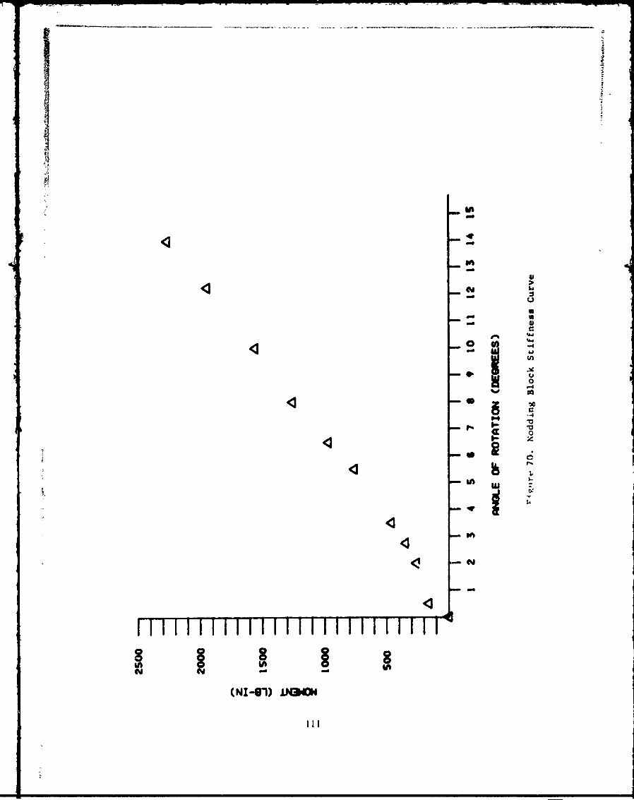
I4
IA
*@
GD
-U
S- S- 6I
444
'44~Ia, .4.4U
04-4
I-
4 0Li a-
q;j'A
4 w4 I
L.
'14c~3
N
II a(NI-Si) JJ43N0W
III
2.1.5 Measurement of the Compliance Characteristics Of 5eg0e0t
ski Covering.
The AIoa model has the capability to account for segment with segment
or sepenut planar surface interactions. In order to perform this
prediction, the compliance characteristics of the selment akin coverings
are required. The physical features of each senmt soft covering can
be characterized by a load versus deflection characteristics. The soft
covering used for the flesh of the manikins consists of a dense outside
layer of polyuretmame or vinyl plastisol molded around a pourous foam
layer of the saw material. As the akin is statically loaded, the vinyl
for deforms such that a hysteresis effect results when the load is
removed. The determination of the compliance characteristics of the
skin covering over pertinent parts of the manikin was the objective of
the tests conducted.
2.1.5.1 Description of Equipment and Techniques Utilized to
Establish Compliance of Skin Covering
The density and thickness of the manikin soft covering vill vary from
segment to segment and also over a given segment. To determine an
average compliance for a segment, deflection measurements vere made at
different locations for that particular segment. If the compliances
were drastically different. as with the front and back of the thora".
then two separate skin compliance functions vere recorded. Exceptions
to this were the hand, foot. and abdomen which were tested at only one
location. All test locations for each segment are presented within the
segment data tables found in Section 2.1.6.2. These test locations were
chosen as segmnt surface areas most likely to contact with another
segment, the steering wheel, seat, or dashboard. Again. because an
average compliance was desired, these test points were located to
include the effects of varying hardware interference as well as varying
soft covering density and thickness.
112
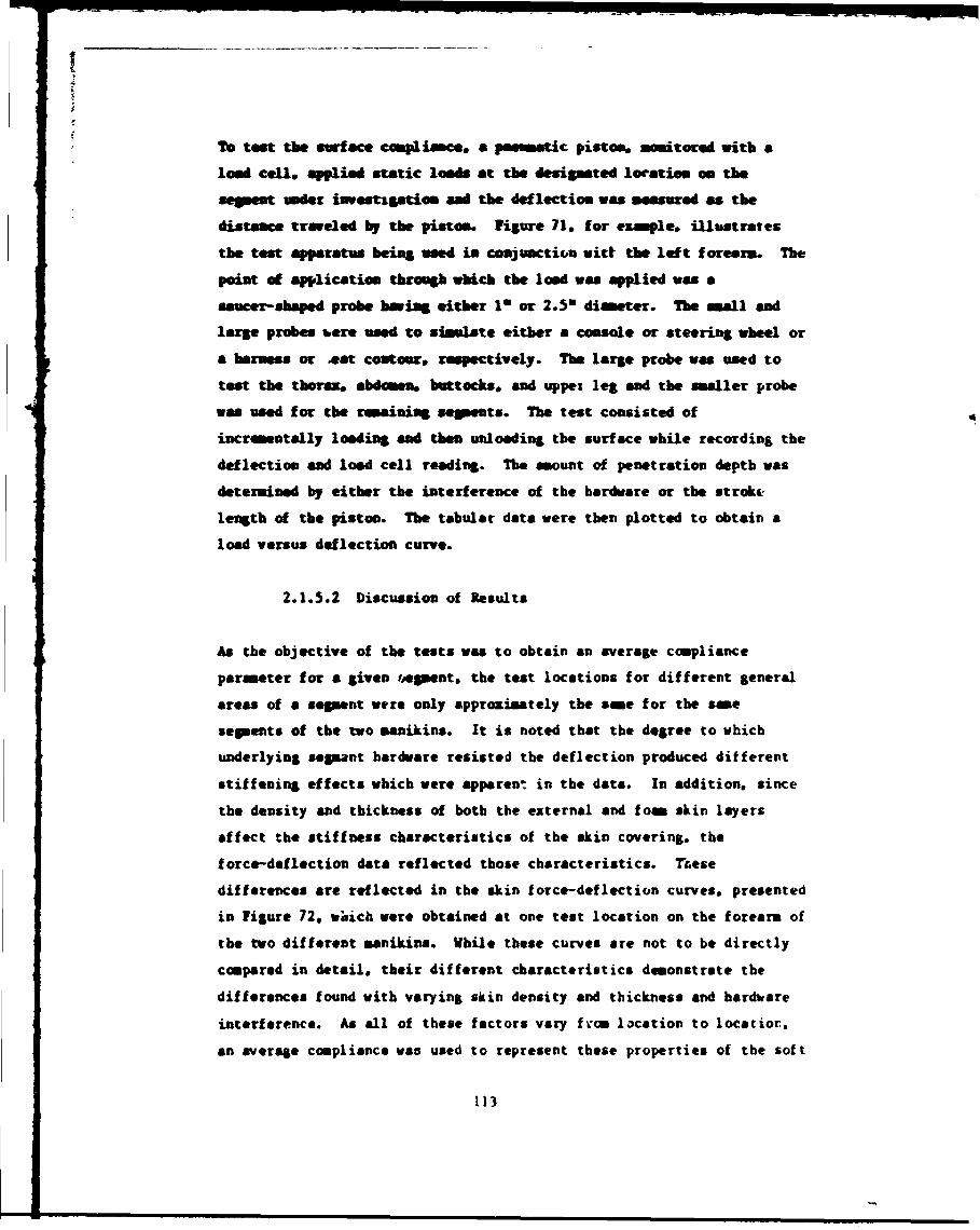
To tet the surface campliame. a pumeuatic piston, mmitored with a
load cell. applied static loads at the designated location on the
sepat under investgetion and the deflection was measured as the
distance traveled by the pisto.. Figure 71. for eample, illustrates
the test apparatus being used in conjunction witt the left foresm. The
point of application throuh which the load was applied was a
saucer-sbaped probe having either I" or 2.50 diameter. The amall and
large probes were used to simulate either a console or steering wheel or
a harness or eat contour, respectively. The large probe was used to
test the thorax. abdomen. buttocks, and uppet leg and the smaller probe
was used for the remaining segments. The test consisted of
incrmntally loading and then unloading the surface while recording the
deflection and load cell reading. The amount of penetration depth was
determined by either the interference of the hardware or the stroke
length of the piston. The tabular data were then plotted to obtain a
load versus deflection curve.
2.1.5.2 Discussion of Results
As the objective of the tests was to obtain an average compliance
parameter for a given fepent, the test locations for different general
areas of a segment were only approximately the sne for the sane
segments of the two manikins. It is noted that the degree to which
underlying segaunt hardware resisted the deflection produced different
stiffening effects which were apparent in the date. In addition, since
the density and thickness of both the external and foam skin layers
affect the stiffness characteristics of the skin covering, the
force-deflection data reflected those characteristics. These
differences are reflected in the skin force-deflection curves, presented
in figure 72. which were obtained at one test location on the forearm of
the two different manikins. While these curves are not to be directly
compared in detail, their different characteristics demonstrate the
differences found with varying skin density and thickness and hardwvare
interference. As all of these factors vary f-om location to locatior.
an average compliance was used to represent these properties of the soft
113
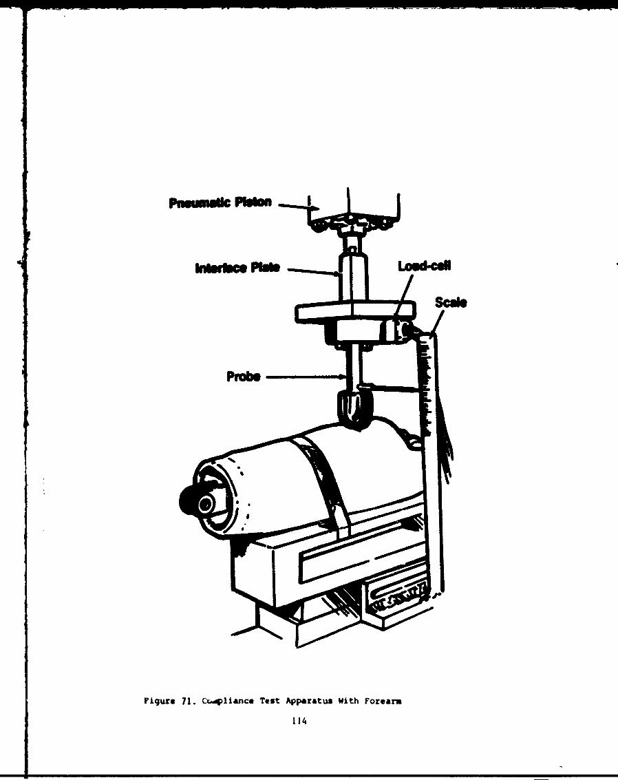
Figure 71. Cr..4liance Test Apparatus With Forearm
114
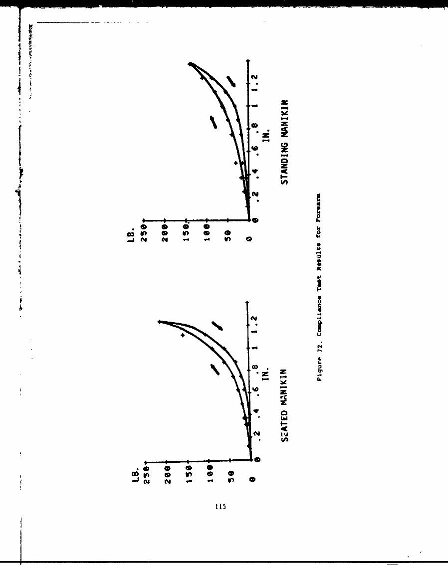
7f
np zto za Cd
z
t %J
CI V)zCY *w -LII ___1N5
covering foir a gives segment. ?be measured data obtained frno the skin
compliance testing are presented in Section 2.1.5.3 for all of the
menikin components.
2.1.5.3 Plats of Skin Cpliance
Figures 73 through 98 present plots of applied force vs deflection of
the skin couerifts for the various manikin segments. From the results
presented in these figures the skin compliance date required for the ATO
prediction program were determined.
2.1.6 Date Tables of Segment Physical Characteristic*
The experimental data describing segmnt properties presented and
discusoed in the previous sections of this report are summarized in the
data Tables 9 through 31 provided in this section. All the data that
were developed for a given segment have been collected and tabulated on
separate pages for easy reference ad use. The description of the
geometric, mass distribution and surface characteristic data for each of
the Hybrid III segments that are presented in the data Tables are
defined in this section. for those segments unique to each manikin
(i.e.. spine. pelvis. and upper legs), soerate tables are presented.
Only ue set of tables is necessary for each of the remaining segments.
which are identical in design for both manikins. for discussions on how
the dat were obtained in these tables, see the appropriate report
chapter.
The following infoirmation is provided for each of the segments in the
Tables:
1. Local 1sf erence Axes. These have been defined to best represent the
symmetry of the segment and are generally based on segment mechanical
features. They are illustrated as a IL, YL and ZL.
2. Anatomical Axes. Identical to segment deinitions in Young. at &I.
[5) end are based on equivalent human anatomical landmarks. They are
illustrated as XA. YA. and ZA.
116
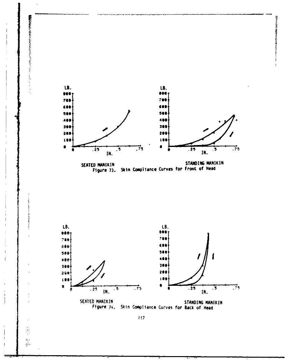
I
LB. LB.seo see,
*00 6o00760 760
* 00 400'
-4004 460300 3g240- 20o
0 .25 . .75 0 .25 .5 .75IN. 0IN.
SEATED MANIKIN STANDING MANIKIN
Figure 73. Skin Compliance Curves for Front of Head
LB. LB.
see,4?00
~5 0Si SW
49e 4061
"361 IS/12G.// -0
a IN. "5 .75 .25 IN. "
SEA1T1) MlIKIN STANDING MANIKINFigure 74. Sk~n Compliance Curves for Back of Head
1!7
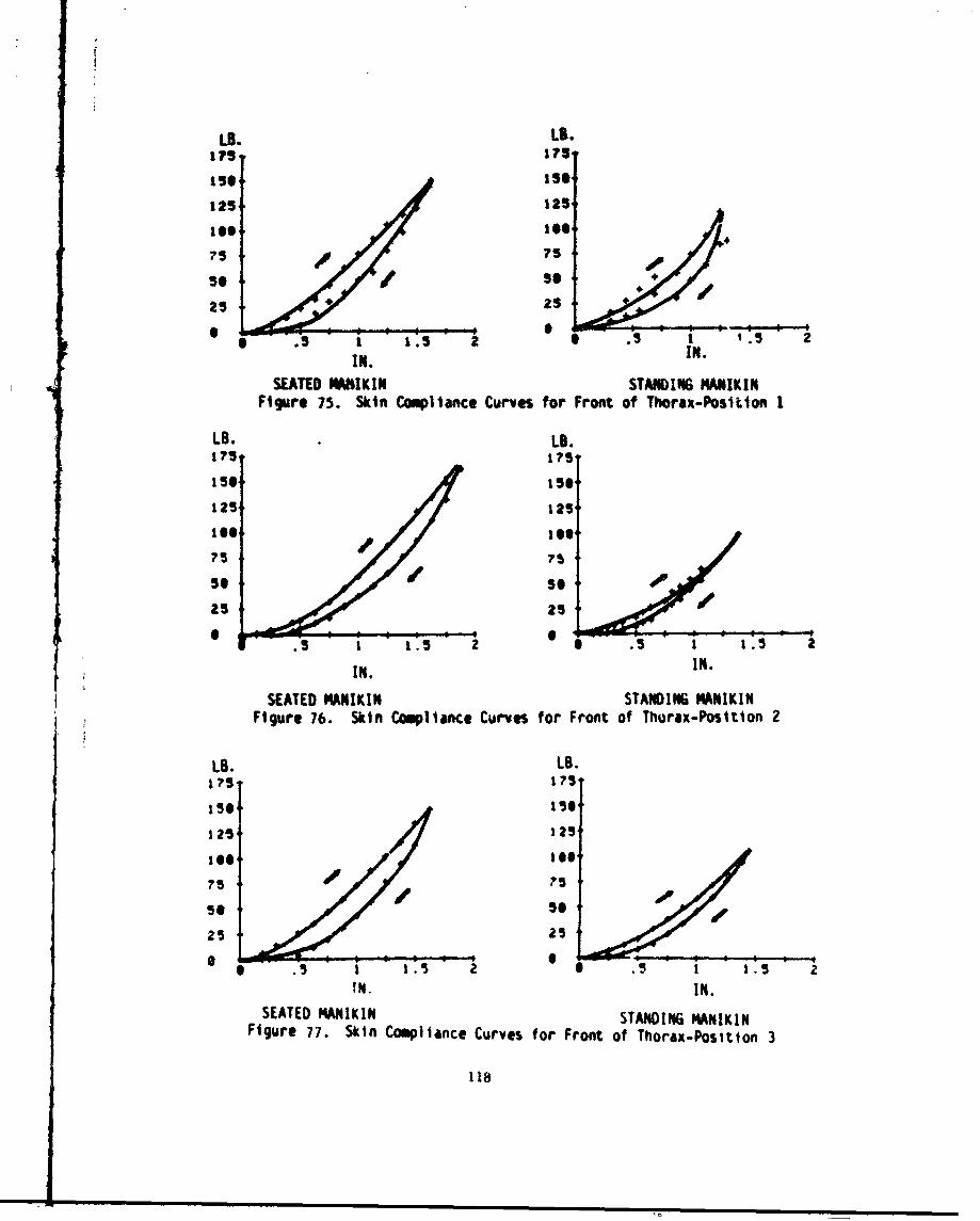
LB. LI.175 1?
25 2575 - 75-
0 0. 1 1.5 2 0 1.5 2l~l. IN.
SEATED WAIKIN STANDING M4ANIKINFigure 75. Skin Compliance Curves for Front of Thorax-Position I
LB. LB.
1501 1561
1 S 125t o o , I S O -T
5 50
25 or25
.I 1.5 2 O .5 1 1.5 2IN. IN.
SEATED MANIKIN STANDING MANIKINFigure 76. Skin Compliance Curves for Front of Thorax-Position 2
LB. LB.175 175150 150
12S4 125
75 75
50 56 Iz0
25 25
O.15 1 1 .5 2O.
ININ.
SEATED MANIKIN STANDING MANIKINFigure 77. Skin Compliance Curves for Front of Thorax-Position 3
118
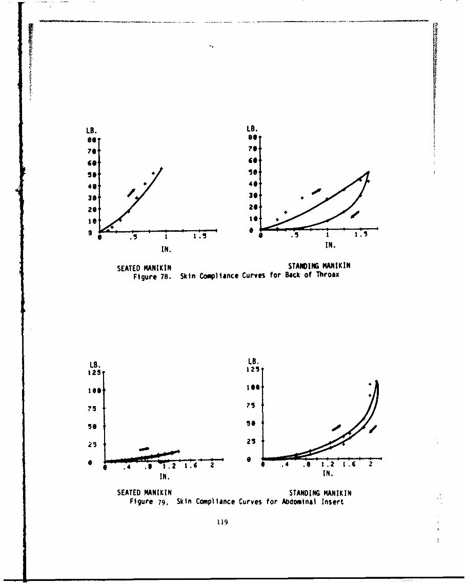
LB. LB.
76 766 66'
46, 4630- 30-J
20 20
et " .1 + . O. 101
IN. IN.
SEATED MANIKIN STANDING MANIKIN
Figure 78. Skin Compliance Curves for Back of Throax
LB. LB.
125 125
166 166
75 75
so 5* 0
25
.4 .6 1.2 1.6 2 .4 .6 1.2 1. 2
IN. IN.
SEATED MANIKIN STANDING MANIKIN
Figure 79. Skin Compliance Curves for Abdominal Insert
119
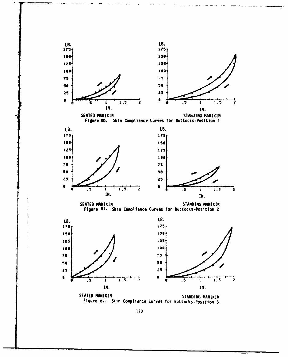
LB. LB.175 175
156 156!
125 125166 lee
75 73op56 5e0
25 25
e 6 .5 .5 1 1.5IN. IN.
Si[ATED MNIlKIN STANDING MANIKINFigure 80. Skin Compliance Curves for Buttocks-Position 1
LB. LB.175 175
156 150,
£25 125,
75 75S. Se
45 25
a .61t. .5 1 1.5 2IN. IN.
SEATED MANIKIN STANDING MANIKINFtgure 81. Skin Compliance Curves for Buttocks-Posion 2
iLB. LB.175, 175
12, 125
0
425 425 * . .
IN. IN.SEATED MANIKIN STANDING MANIKINFigure $0. Skin Compliance Curves for Buttocks-Position 3
120
to o
so. .lo
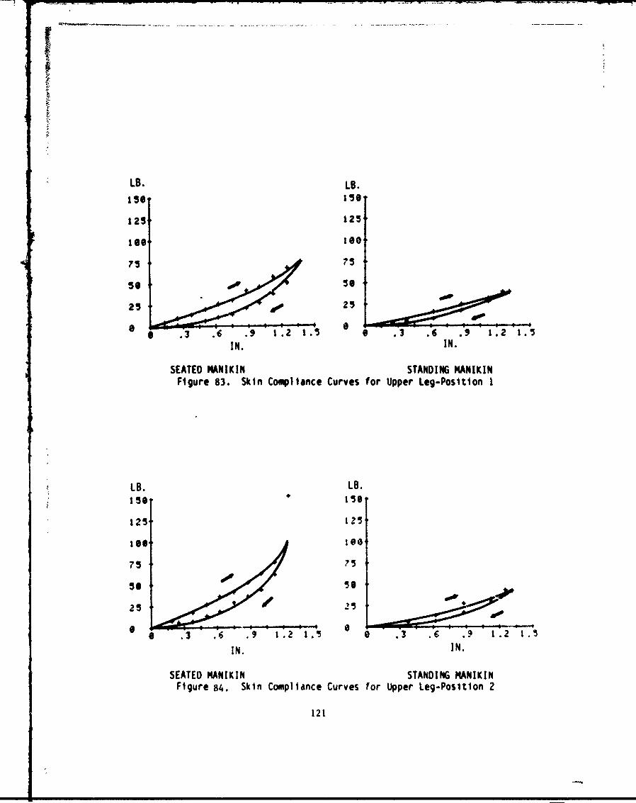
LB. LB.
156 1560
125 125
tee Io
75 75
25 25
6 .3 .6 .9 1.2 1.5 0 .3 .6 .9 1.2 1.5IN. IN.
SEATED MANIKIN STANDING 1ANIKINFigure 83. Skin Compliance Curves for Upper Leg-Position I
LB. LB.
125 125
1oo, 10
75 75
252
.3 .6 .9 1.2 1.5
IN. IN.
SEATED MANIKIN STANDING MANIKINFigure 84. Skin Compliance Curves for Upper Leg-Position 2
121
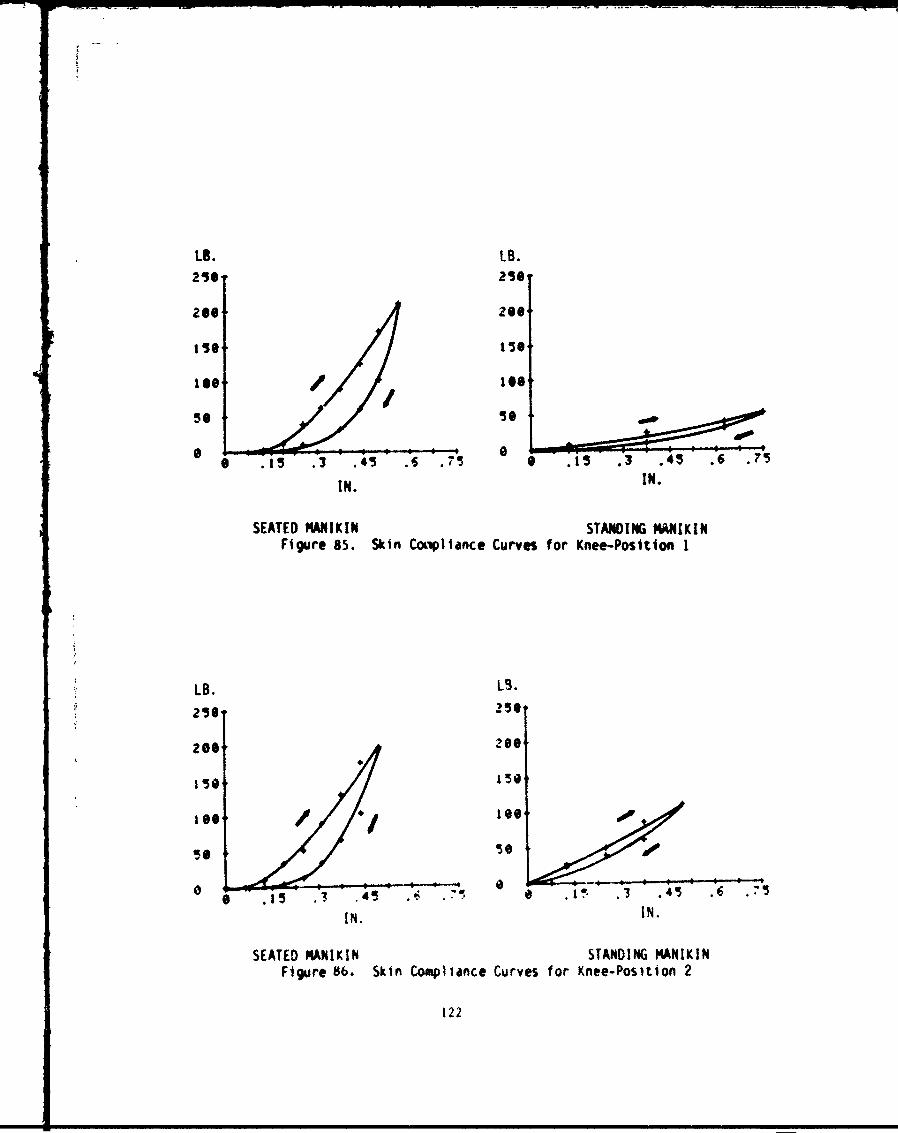
LB. LB.
150 150'
50e 50
6 .15 .3 .45 .6 .73 0 .15 .3 .45 .6 .73IN.IN.
SEATED MANIKIN STANDING MANIKINFigure 85. Skin Cotpliance Curves for Knee-Position 1
LB. LB.250 250
200 20
150 150leo / *10
50 SZ30d
* .15 . .45 .
IN. IN.
SEATED MANIKIN STANDING MANIKINFigure 86. Skin Compliance Curves for Knee-Position 2
122
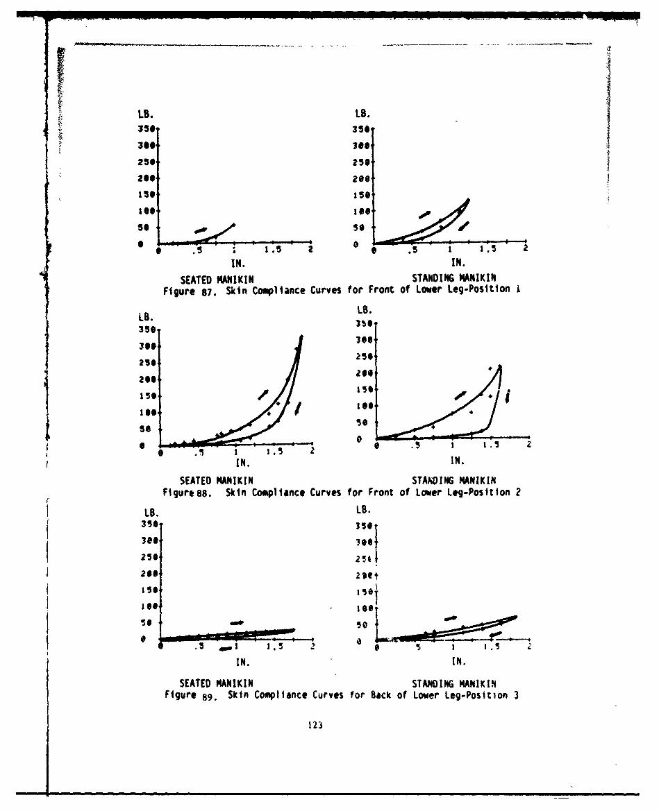
,2 LB. LB.13 0 350
300 3e0
250 250
200 2e0
10 05
0 .5 15 2 0 .S 1 15IN. IN.
SEATED MANIKIN STANDING MANIKINFigure 87. Skin Compliance Curves for Front of Lower Leg-Position I
LB.
300 30030
250 25O
200asis* ~
56 56
0 a O 1.5 IN. IN.
SEATED MANIKIN STANDING MANIKINFigure 88. Skin Compliance Curves for Front of Lower Leg-Position 2
LB. LB.
350 356
250 2I
200
Is$ 15.1Ise Ise T
IN. IN.
SEATED MANIKIN STANDING MANIKINFigure 89. Skin Compliance Curves for Back of Lower Leg-Position 3
123
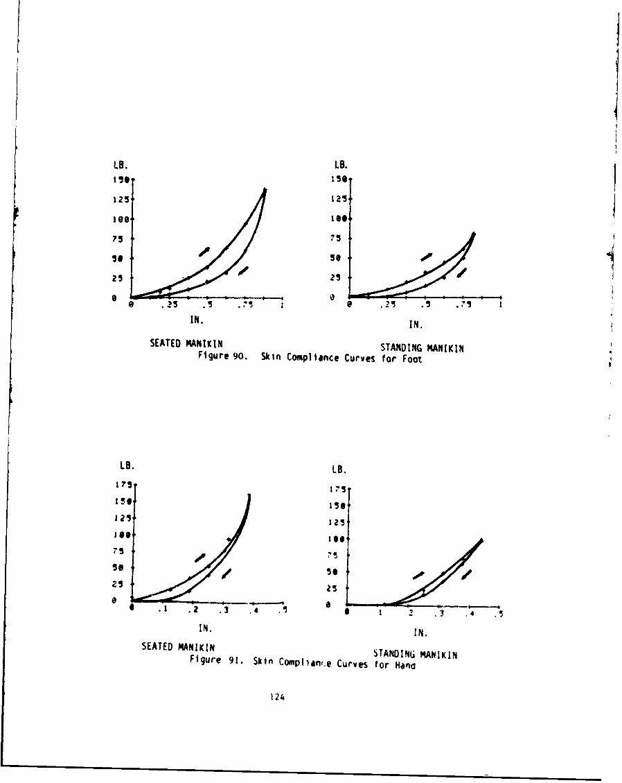
La. LB.
125- 125
75 7
0. 5.
2 .25 .5 .25 / 23
IN. IN.
SEATED MANIKIN STANDING MANIKINFigure 90. Skin Compliance Curves for Foot
LB. LB.
1751'1 5 0 1 5 0 1
12! 1251
25 25,
IN. IN.
SEATED MANIKIN STANDING MANIKIN
Figure 91. Skin Complianr.e Curves for Hano
124
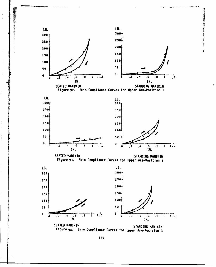
LB. LB.
256 230
206 200
so 56so
S .2 .4 .-. .26 . 4 *4. .
SEATED MANIKIN STANDING MANIKINFigure 92. Skin Compliance Curves for Upper Arm-Position 1
LB. LB.300 l6e
1506 4
0~ .2'---- .4
IN. IN.
SEATED MANIKIN STANDING MANIKINFigure 93. Skin Compliance Curves for Upper Arm-Position 2
LB. LB.
136
Ise if#06
a .2 .4 . .8 a . . . . .9 1 1.2IN. IN.
SEATED MANIKIN STANDING MANIKINFigure 94. Skin Compliance Curves for Uipper Arma-Position 3
125
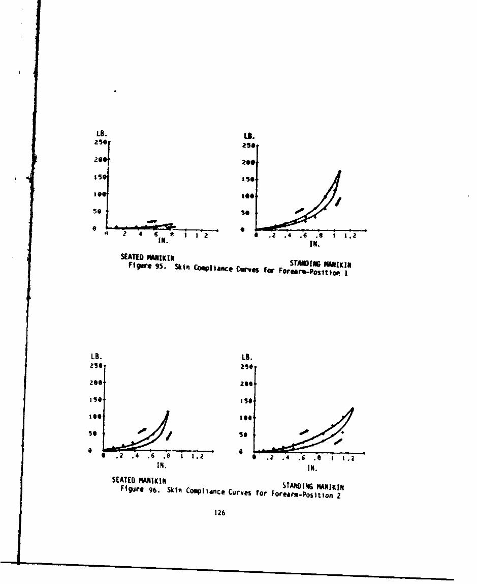
LB.L.
20 200
is lee
0*~tP:% 0 lo 4 484 z 4 6IN tI12 a .2 .4 .6 .8 1 1.2
SEATO MANIKIN STANDING MANIKINtFigure 95. Ski" ComP)11nCe Curves for Forearg-.posttl 0 I
LB. LB.2150 25
200 2004
40 is
0 .2 .4 .6 .8 1.2 0.2 .4 .6. 1 1 .2IN.IN
SEATED M4ANIKIN STAND14G MANIKINFigure 96. Skin Compliance Curves for Foreirm-Position2
126
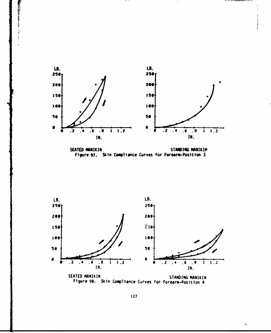
13. La.250 256
200 20
lOOtoo +
5e0
6 .2 .4 .6 .9 1 t.2 0 .2 .4 .6 . 1 1.2IN. IN.
SEATED MANIKIN STANDING lNAIKIPFigure 97. Skin Complince Curves for Forearm-Position 3
LB. LB.
250 256
200 200
,.A,0 .2 . 4 .6 .9 ~l. .4 ft. .
IN. IN.
SEATED MANIKIN STANDING MANIKINFigure 98. Skin Comliance Curves for Forear-Position 4
127
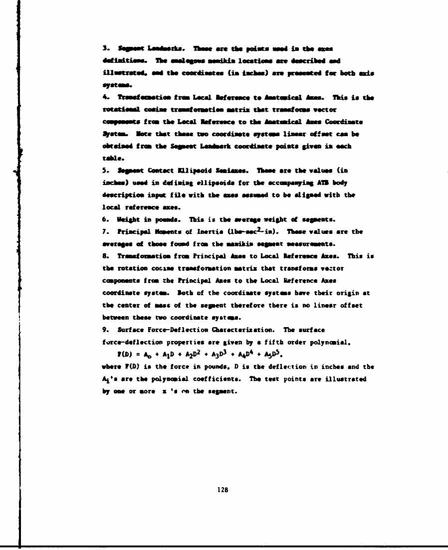
3. Sgmt Laghcs. These, awe dhe puots use is the aw
definitions. The amalegoss mmkin locations amre scribed snd
ilntroted. an the coordinates (in tachas) are, pueted foe both adms
systies
4. Trawe~setim frm Local Ref erence to Anatmical Ames. This is the
rotatinl cosim trnouintion matrixthat trawstoems vector
cmonns f rum the Local Ref erence to the Anatomical Anne Coordinate
System. Note that thus two cordite system linear off set: can be
obtained fre the Soonest Ladark coordiate puints given in each
tamle.
5. Sepiest Contact Illipsoid Seminss. These are the values (in
inch..) ueed in def ining ellipsoids for the ecco.pamying AM body
description input file with the eaes assumed to be aligne" with the
local ref erence azes.
6. Veiagat in pounds. This is the averae weigjat of segments.
7. Principal flimets of Inertia (lbw-sec 2 -iv). Thuse values are the
swerages of those found from the masikin seWent measurmnts.
8. Transormnation from Principal Anes to Local lteresce Axes. This is
the rotation cosine transformation atriz that transfoiss veztor
components from the Principal Axes to the Local Reference Azes
coordinate systes. Soth of the coordinate systows have their origin at
the center of mass of the sepent therefore there is no linear offset
betveen these two coordinate systems.
9. Surface Force-Melection Chaacterizationi. The surface
force-deflection properties are given by a fifth order polyaosial.
F(D) = Ao 4 AjD + A2!)2 + A3D3 + A 4 + A0D.
where F(D) is the force in pounds, D is the deflect ion in inches and the
Als are the polynomial coefficients. The test points are illustrated
by oue or sore x Is rea the segment.
128
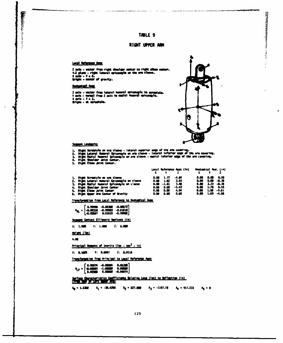
TOLE 9
I a" - "No from n9 ot~i a1 to "ft Sam Cace.
W to e mouo a samLmo
3190. - ma o f lWy.
vales - weool (n IM toee mieI t %am e wfta.
1. "S"6 mcfale do we slowe lateral Suener sov of the &m Semil,2. motLow anWS -SF1 f~lmad ams slamwe. ltel Inferfer up2 tft . Cowes.3. Iff 111ofe, 01msi Etcom.le so ago 0~ev - motel Saft~e op of the on Cowles.4. stt Shoulde Joist Ceate.
.61fl Du Joit aft er.
tWA. cel foreac An$ Is) Anmial A n
1. Not6 Acrinale an w slae 0.16 1."1 -4.06OA 0.0*6 0.002. in ateral evempot bice: lo: SIN" 0.16 1.62 3.4 0.66 0.6 406
3310c t~al ftmral 1,1~l sosa 0.66 -1.61 3.6 6.0 L.13 -L30. 196 sw Joist Csate 0.0 0.06 -S.43 0.6Lo s .11AS. 31ot amv Joist Centel 0.06 0.06 4.94 6.0 1.99 49.01
6.*9Mebn~a6~fatty 0.06 0.O LO 0.00 06 1.69 .6
Trmetf!l from Local "Pf go" t W mWiCI hme
AA .. I 10 4S.99903 06151S1LOW39 0.61519 -8.99981J
%eMRa n esut (lllosig Sl~ai (Ia)
1: t1006 Y: 1.080 1, 6.0
4.66
priaclsel ftwsi of Isertta (166 . Set al14
3: 6.11f V: LO099 2: 0.0116
lriaftnl Meriacimal to Local bfW~min
r 6.9007 408894 *.umi*t 14.6661 .1.~66 LOOM66
A -1.6113 A e 3L& A, * MAN A.3*e1191.10 At -911-233 A 0
129

TABLE 10
LEFT UPPE IM
I ais * 'VM frm t left *mldr tgala. =S lt f 4y1bW Ul,.142 pla - left newq 69tV0iI on tw amDoi.I ads - v a L
"iOsl - secto trn lata Iww*, GPlcem~I to O0 tato.1ants swa m 04141 %MW-a 410h. e~o'11 to N IlS.
Oral% at sonMs
igof- t Acrmall.MSm"-Itriasw fti eCw
4. Left 3*szlaw joint Center.S. Left MOM Joint Centor.
a& fereaco Air@% (4) Anatical Bitt (in)I Ir I I I
I.left Atreeleo aft ese 0.00 *1.17 .4484 0.00 0MD 0.003. Left Lateal ielf~l flICoa1 o t"~ 0100 -14u1.5A4 0.00 0.0 4.36L. Left ftoal 0Ar01 (OtC4Pi0l an 1oese 0.0 1.41 J." 100 -M3 4.3A. Left Skuldsr jetat ceetr COO Ms ..S-.1 0.00 -t. is o.$S. %Aft 1* Joint Center 0.46 906 4."4 0.00 -1."9 .9.816. Left VOW *a comter of srewttl 0.00 L"~ 0.0 l0.00 .1.0 -4.58
Thfoerntip frn LkrA? Sfroe to Batl AIe1
A,% CAI L64993 181,1 -LOWSS .. 018 .*.19961
3: 1.9. f: IA"0 1 6.00O1
I~ .)J f:0.099? 3 0.0116
Traof.0112 fros 'tuclool to ~cI bofrgee Awn
W mqr ace agO ltics caeffutc es !jleS-f to" Nfroo(Ia
%.le.I3I A 3~5U A-s g69 A.*.~s AS As a1*:
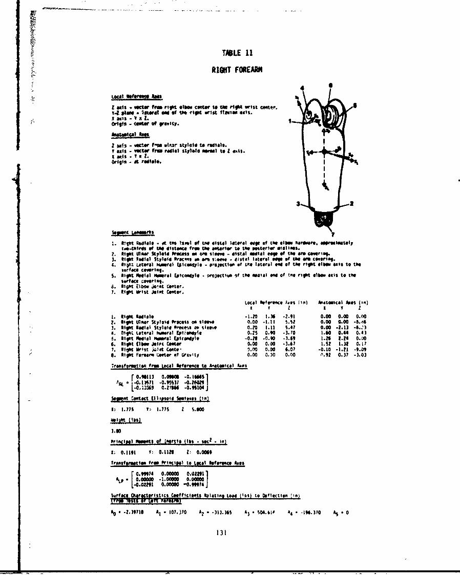
TABLE 11
RIGHT FOREARM
I axts *wcw Iram riowt ele. cu~ £ t .Viaplt anist Cono.Vt4 flow9 - l4tft a" of V*mf lot welit Itontom .us.x axis - V L
ori as 4 Of gravity.
Z gts - vener 1" mtse st3ltd to rait.T axis - vecto Irim radial 11,116,1 morgal to z emls. '..1 ants T x Z.oriliq t £ raele.
3
A. R" Q*d41@ - 4t tv* ISuM of tme disel lar*rhl OOV of thme lift eartee. apealmssl,to-tmtres at tme distuince Irm the ater o the. Posterior idlimes.Ri Bght Itmee Sty1.d PrOces -4 4M sle,. ditilul Raial top of thme amn ceeris..
3. tigh Uaia Stpbeid praqs~ 00 uft s-eAwe tilt&! lateral giqe of tme an covertm".4. llqr'. Latel Kert I'ini I tcosdjlo piojoCtoo of Lts lattr~i *no of lime right *low "31s to tme
Surf ace C~1.fe.9. 11;4 t dlal Am~ral £Dtcceijrl@ - grjectim of thmo 8141@W of tne right elbow ais to lime
surf ace coverisq.i. alip. Mom0 joe Catesr.7. Rtfit Wrist Joift Cotte.
Local ImfVeece !it$ (in) ialtcal Ages (14)
I. light Rh14l9 -1.20 1.36 -2.91 0.00 0.00 0.002. light t10e' S11014 Process as sleeve 0.00 -1.11 S.S? 0.00 0.00 *Sat63. RIt Radial Stylole Prs'nS as %1# 0. z0 1.11 S.AY 0.00 .2.13 4_1.34, Clt wetrai *wmrat lot.-sho5le 0.29 0."0 -3.10 1.60 0.44 0.43S. hlySt ftesl himon? EPCW411#yl -0.21 -0.90 .3.69 1.26 2.24 0.006. Right (lb.. Jolp Coer 0.00 0.00 -3.67 1.92 1.38 0.177. 11lo~t Wrist wsat Until- 1.00 0.00 6.07 -0.10 -1.41 -9.09a. Righ" feowee'q t*.tor 00 Gravity 0.00 0.30 0.00 r'. 92 0.37 .3.03
T'ressfof"Io from Local Referece to &dl.Ical favs
u. 169 W .21164 .0."106
5tefat Comtect (Illpu"oIs Usot*ose [to)
I., 1.7S V, 1.779 1 Mm80
weulo, (Ibs)
3.30
Pelecipol VMONS, Of InetlS (lb1% . MK ain
1: 0.1191 1:, 0.1128 Z: 0.0ant
TramtsfM14011o frai OriecIP4l to IoAl 1fereeCO An*%
AL 0.999000 .I00000 0.00m91Ap 0.99097 -0.00000 0.000901
10.02291 MOW00 -0. 911114
qraClt ristics Coefficients kjlatime L044 (16%) to Defitrtion ~n
A0 2391 A1, 107.370 A2 . 3339 A3 * 'A461- &4 -196.)10 A9S 0
131
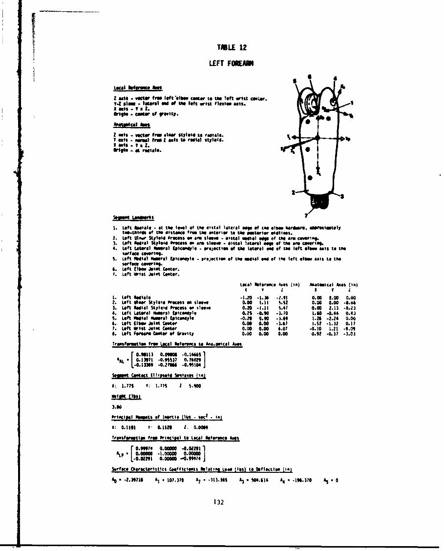
TMLE 12
LEFT FOEAM
5SLocal !!fLow"e AN$
z amts . vecto free left *elbas Center to tad left .1st cespor.1-I plen - lateral ami of Ite left Wrist fla216 axis.I anls V x 2.
tons - =inte Cf gravty.V
bAatial Jbin
I axis . vector free (A1w Styleld to [email protected] acts . *~mo free Z &It to radISl St.0otd. 'Orton a at radiate.
2
1. Left lagialt at toe Ieve of tre aistal lateral "I* of Efte ellse hrure. akw"Iumatetytonp.tillres of S dtsusce fron tue aeeIa to to Mstartar eldi lees.
2. Left glowr Stylotd froceams onarm sleeve -distal modmlt sp of t"e arm Cewrttg.3. Left badial StYlete d eu P* S S arm %lIwo . istal !atoal osp of the arm CMISt394. Left Lateral feral ICOIgl orejectfon of toe lateral asd of toe left elbm. axis to the
sofie cowriS.S. Left Olmal Umeral tolceseyle .projection of toe M414l 0od of the left elbe axis to the
suerface covering9.6. Left (tb"e Joist Center.1. Left Wrist Joint Center.
Local Reference Ames (in) hutmIcal AMOS (in)A IFV I I i
1. Lef t Radilt -1420 -1.36 -1.91 0.00 10.00 0.002. Lef t Wiser Stjrleld Proceus as sleeve 0.00 1.11 S.S2 0.00 0.00 *4. "3. Left Radial $tjitod Process so sleeve 0.40 .1.11 5.41 0.00 2.13 -8.23A. Left tLateral Himerat Epicoseys 0.2S .0."0 -3.10 1.60 -0. " 0.43S. Lett Oedta 01101111at EVICsd11l .0.23 0."0 -J-69 1.26 .2.24 0.006. LefIt Elbow Joist Caster 0.00 0.00 -3.61 1.32 -1.32 0.117. Left Wrist Joint Caster 0.00 0.00 6.07 .0.10 1.21 -9.09S. Left Foearm Cester ef gravity 0.00 0.00 0.00 0.92 .0.3? -3.03rasfsremtis free Legal lieoersc to MAIIco LAe
AA !.13971 -..9137 0.?60291.0.13309 .0.27964 .0.95104 J
Sesmt Contact (111"004 Wsaves [in]
1-, 1.77S Y; 1.17S I 'iWO
3.80
Artacil! ot uesets of Iaerta flbs - soS -In
1: 0.1191 1. 01128 1. 0.0069
lrassferutaso free Orlclpsl to Local Referonce Ames
r0995 0.00000 .U2m1At, 0.0600 1.0m00 0.00000I
10091 0.00060 -0.99974
Surfaco Cllrctqristics Coefficients holatt!2 Load ilbs) to inflection (101)
-2.39711 A, 9 107.310 A? - .311.39 A3 S 04.614 At - .194.310 AS 0
132
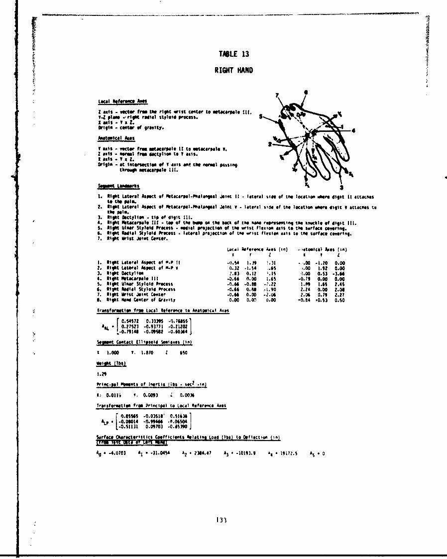
RIGHT HANED
Local Rotorence AMe
Z axis - vectore fr the right wrist center to metacarpal. Ill.1.2 plan . right radial stjvloid process. %I axis - V x . %origin - Comter of gravity. *
Anatomical Axes'
I axis - vecor frog wogcarpale I I to uetscarpale V. £Z axis - norml from dactjllon to T WxS-I axis - T x Z.origin - at intorsectien of Y axis ae thme nomal passing
through metcarpal. Ill. I
1. Rioht Lateral Aspect of l~ltacerval.Pnalangal joint it lateral lifta of tne location where digit 11 Attachesto the palm.
2. 1101t Lateral Aspect of i*tacarpal.Phaiengal Joint V lateral side of the location Mfgr digit V attaches tothe pole.
3. Right Gectylton - tip of digit Ill.4. Right Fatacarpale Ill - top of the bW# on the back Of the *a"i representing the nckle of digit Ml.5. Right liunr Styleid process " mdial projectian of thea wrist fleuion ais to the surface Covering.6. light Radial Stlifd Process. lateral projectiont Of the wrist flezIOn aIS to the Surface covering.7. Ight wrist Joint Ceoster.
Locai Wserence hses (in) .- '.tomical Am*$ tin)
1. Right Lateral Aspect of NP0I .1).S4 1.1J9 .31 - .00 .3.40 0.002. Right tateral Aspect of NP V 03.32 -3.54 .6-.00 1.91 0.003. Rioht Dactylion .83 0.1? ~.IS ).00 0.53 -.. "4. light motacarvalo Ill .0.66 0.00 3.6s -0.79 0.00 0.00S. light Ulna Styloid process .A.M -0.68 -11.22 1."9 3.6 2.456. tight Radial Styloid Process -0.66 0.6 44 1.90 2.24 0.00 2.047. Right Wrist Joint Center -0.64 0.00 .0o 2.06 o.7g Z.27S. Right hlad Center of Gravity 0.00 0.00 (3.00 *0.84 tQ.Sl 0.50
ransorma ionfrog Local Reference to Antatomal& Aie
Maw557 0.3339 -0.76855IS0.252 -0.9371 -0.120AAL ~o.?148-0.09SO2 -. 06
Segment Contact Ellipsoid Somiases (in)
I 3.600 1. 3.810 2 65
Weight (Ibl)
3.29
Printc-pal fwomnts of Inertia (IDS - SeC2 -11:.
1.: 0.015~ T. 04G03 z 0.0036
Trisformation fro Principal to Local Reference has
[ *ISG 0.03S16, 0.5336AI 00014 -Mom a4 .6.G54
CoefiietsMoat4, Load (16%) to 0oflect ion (in1
#V a 4.310] A, -31f.04S4a 42 - 23$4.47 A, - -10193.9 1a *i8(7.S A5 0
133
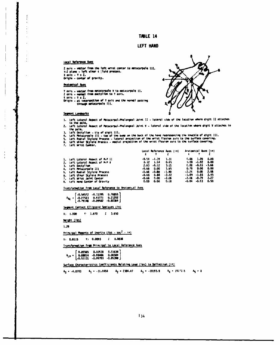
TMLE 14
LEFT HlAND
Loual Rf greace Axis
Z axis . vecto from Va left wrist cantor to maacarrale it[V.Z vlam . left viso 5 -,-lai proces.I axis - V x Z.oriole - cantor of gravity.
Aatmical AWSs
V axis .wec"4ifrom tcramldV to tacrpole 11. 4 \Z axis . *WIn free gactylient to T axis.X axis - V x Z.Origin . at incorsactiea of V axis and tlie mnral passing
Sw~et Loeft!$
1. Left Lateral Asgat of iftcarpal.Pftalsngae Joint tl . lateral side of tiSo location Offire digit 11 ittaClwsto the Pal.
2. Left Lateral Mwpct of atcrl.aana Joint V - lateral Side Of the location 11014fi digit V attactcs totIo 0alm.
3. Left Cactylien - tip of digit Ill.4. Left Aftacappole Ill too of ta bum on tea Wait of the fland regrabonting the knwckl* of digit Ill.S. Loft Radial Styleid Preoesi lateral Projection ot tfo wrist flexion axis to the surfac caoring.6. Loft visor ftylaid Process ON6 mailprojection of tP* wrist floxuon axis to the surfae cowingo.7. Left wrist Center.
Local Rference Alt" (I A) Anatemical Ages (in)A Y I
1. Left Lateral Asoect of M.F 11 *O0'54 .1.34 1.31 ".00 1.20 0.002. Loft Lateral Aspect of P-0 V 0.$2 1.54 O.AS 9.00 .1.91 0.003. Left Dactylien 2.6) .0.12 M.S C.00 .0.53 -3.640. Left Pvoacapala Ill -0.66 0.00 1.6s o.ig 0.00 0.00S. Left Raial Stjtloid Process .0.64 .0.06 -1.10 .2.24 0.00 2.0616. Left Offer Slylaid Process -0.66 0.08 -2.42 -1.89 .1.6S 2.457. Left wrist, Joint Center -0.66 0.00 .2.04 .2.06 .0.79 2.27S. Left fland Center Of Gravity 0.00 0.00 0.00 -0.84 -..5 0.50
Transformagtion fr o~ Re1*1ferenc to h'.tousLal As
r .. 4S72 -0.3339 0.16055*~ I 4.27523 0.931?1 0.21202
-..714 .0.09562 -0.60364J
SOW011 Cotact (lli9561d lemas#$ Oft)
a. 1.000 1, 1.670 1 3.650
Weitht Ibsi
1.29
1rinCIP41 ftnOts of Isortia (lbs_ Satz .In)
V: 0.0115 7 0.0093 1 0.0014
Transfermtien ftV Pflaclpal to Loal Reference Ames
r .85565 MAN51 0.516)61
surface Charoctoristics Coefficients ftlatfne Lwd (160) to 00flectten 041
AO .4.0703 A, - .31.04S4 A2 o 2)64.47 A3 a -10193.9 A4 - 191'?.$ AS 0
134
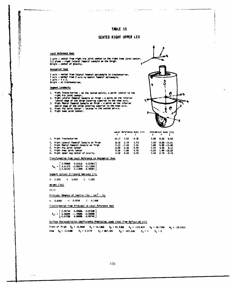
TALE 15
SEATED RIGHT UPPER LEG
Local RtftrenCO Axes
Z axis . vector from right hip Joint center to the rigt khe joint center.Y-Z plane, rigt lateral femril condyle on th tWigN.Origin - center of gravity.
Anato ical RAgqW
Z ais - vOcto from lateral few&a spicoadyle to trCisemterion.I ais - ral frm Z axis to medial fow al eicodyle.I axis . y x Z.Origin . at trochafterion.Selmt Lanmrks
1. Rtght T hm erin cen the seated pelvis. d point literal to theright hip joint center.
2. Rigt Lateral Fwial Cn4dyle on Thigh . a point en the inferiorlateral "tle of the tXhg Covering uaperfor to the knee Wi. Y 114P
3. Right We)il Few#l Co I an Thigh - a point isn the Interiormedial eg of te taitg covering sipertor to the knee axis.
4. Night NIp Joint Center - located In the watod pelvis.S. tight Ks"e Joint Center. 26
LOW OI Fet ce Ae Oft) Anatomical Ages (in)I I I
1. R1 "t Trochenterion 0.17 3.9? -9.36 0.00 0.00 0.00
?. Right LUteral Fowmenl Coadyle on Thigh 0.16 z.39 S.93 0.00 0.00 .15.411. Right ftdlal finoral Condyle on Thigh .Z3 -4.89 5.40 q.00 S.00 *|5,4.4. Right IP Joint Center 0.00 0.00 -9.96 0.44 3.4 0.125. Right Kne Joint Center 0.00 0.00 6.S6 -Q.29 1.99 -16.286. Rignt Upper Log Center of Gravity 0.00 0.00 0.00 0.00 .18 -9.76
Transformation fno Loco) Refeence to natoemical Aes
[0.01370 .0.99275 -0.1140L-0.012 0.11909 -0.099145
Segment Contact (llhPigid ,,letes CIA)
I: Z.950 1 3.00 21 Y.285
33.11
Principal he ts of Inertia fibs - sicz . in)
1. 0.6092 v: 0.5934 1. 0.1064
Trnstformation from Principal to Loco[ Reference AL*
0. .99740 0.0000M .0.072061L -0.0;S -1.0=O -. OMgt
$uface Chaacterititcs Coefficients Predicting LuOt (1b4) from ofiectimn Ain)
Front of Thigh; % * .0.1644 A, - 14.1844 A2 * $1.931" A3 a .122.6Z4 A4 .96.1296 AS . .29.0903Knee A0 . -.014 A, -. Zi214 Az a 8#.34 A) , -401."9 A 4 .1 A . 0
135
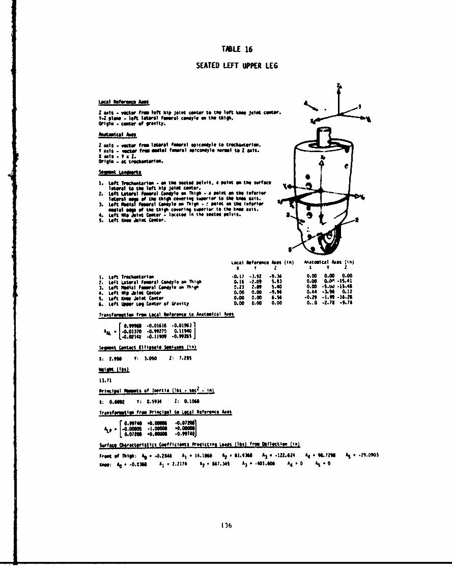
TMLE 16
SEATED LEFT UPPER LEG
Local Itae Ams;s
Z axis .wctor tram left nip joint center to the loft bwo joist cavter
Origis Cantor of gravity.
Anatomical oAm
z "is . ooW from lateal femoral epicosd~le to trochastrlas.V axis wette frau "ial femoral apicasdYlo sormel to I aSRI.I axis - I x 2.Origin - at trackasterion.
1. Loft TrOchaOStOrt . as the Satad Pelvis. a 0014t as tho 110facolateral to it"o loft ht joist castor.
2. Loft U~tarl ftW4l Cas4*lo as Thigh - a Point as the Inferiorletorl wase of tne thlo Cowring seolor to the u tasu.
3. Left mftal ftae Coet* OR Twib"s .point sto Iferiorseal "il of too taig vmcowl"~ superiv to tat ones axis.
4. Loft Nip Joit Cnter. -ocate inthesated plvis. 3 I'S. Left Kws Joist Castor. ~.2
Local Ilforasce Am 0 m) AWOReatcl Amos (in)a 1 2 1 V I
1. Loft Tractastoa -0.11 -3.92 .9.36 0.00 0.00 0.002. Left Lateral Femoral Coneylo an Thiqb 0.14 -. "0 5.93 0.00 0.0" .15.413. Left Y4Wul Famoral Casaylo am Tigh 0.23 2.W S.40 0.00 *5.W -15.484. Loft NIP Joist Caste 0.00 0.00 -9.94 0.44 -3.94 0.12S. Loft 9m joist Centor 0.00 0.00 4.34 -0.29 -1.99 -14.284. Loft Uper Leg Cestor Of Gravity 0.00 0.00 0.00 0.10 .2.76 -9.74
TraxSform trea Loca nforsco to Anatasical Axs
AL 0 .999 .0.0141 .0.019631AM 4.017 .0.99279 0.13940
Set Castet (Illseold lSoigm t in)
1: 1.969 7: 3.0%0 Z2: 1. 28
"lot 011111
13.11
principal Poets of Inrtia (lbisc - Is.)*
1: 0.44m 1" 0.3934 Z2: 0. 106
Traasfeeautlas frau Principal to Lustl Reforeac Ao"
.[.0.99740 #4.08m;004 ym
AL l0oom -1.00 *0 OfiffifJ
suate 04ractorlsat'c Cofflctosta ProctlIn M&46S ts) from Oviloc~tiasl's
frast of TW, All a .0.2844 At * 14.118424 43.3934 A36a .122.424 A4 IL 97296 AS * M9093
£50: ..00 4 A, a.2174 A2 a "7.3 A3 9.401.406 A4 o0 Ae 0
136
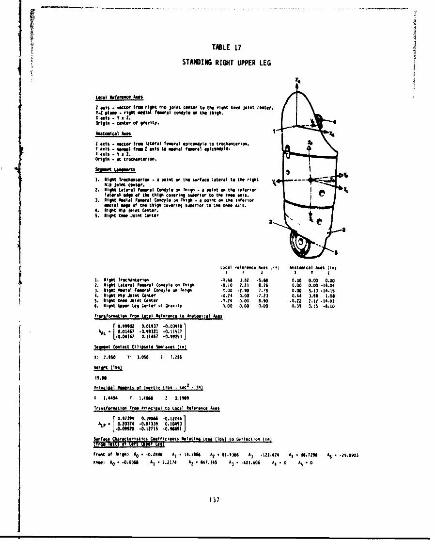
TABLE 17
STANDING RIGHT UPPER LEG
Local Reftrenc AmeS
z axis - vector fro right hip joint center to the right thee joint center.V1 plane - right "edial femoral coadyle on the tigh.I ats - V I Z.Origin - cemer of gravity. 4
Aatomical Axes
z "is - voctor from lateral femoral ep#lconl* to troclnt eron. .V "ils - eI from Z "is to "dial fa arla epicaYIle.I ail - T a Z.Origin - at trochanterion.
1. Night Trocinerion a point on the surface *ateral to the right -. h .hp joint center.
2. Right Lateral Femoral Codyle on Thigh - a point on the inferiorlateral eip of the thigh covering suprior to the kne axis.
3. RIoht 1odial Fsmral CWoayle on Thigh a point on the inferiormedtal eWge of the thlgh covering soperior to the Inee axis.
4. light Nip joint Cmer.5. light on Joint Center
Local 4#10refte A*% 111) Anatomical At*% (InjI I I a I
1. Night Trochateri n .- 3.82 -S.4 0.00 0.00 0.002. tight Lateral Femoral Condjle on Thigh -0.10 2.21 6.26 0.00 0.00 -14.043. Right Redial Fmwra Cendyde an Thigh (% 00 -2.90 ?.4S 0.00 11.13 -14.114. light NMp Joint center 4U.Z4 0.00 -7.23 0.44 3.9i 1.08S. light KAne Joint Center .n.Z4 0.00 8.90 .0.20 Z.d -14.926. Right ti*er Leg Center of Gravity 0.00 0.00 0.00 0.39 3.1s -6.10
Transformation fr!! Legal Reference to M~itootcal Axes
r.992 0.01937 .0.039701[0 :01441 .0.119321 -0.1153?,0.0417 I0. 1144 -0.9M2I
selmt Contact (llipsoei somlaes (in)
1:' 2.M0 V' 3.00 1: 7.ZI
well" (Obs]
19.94
Privicital _Pwntl of Inirtic (lbs - ic2 - iAn
11 1.4494 '. 1.49 , z 0. 19
TransforMatIOn Frog Pr'inC*Pal to Local 10efeenc Axes
o.91M 0.19046 -0.14zz41ALp . 0.20374 -0.911339 0.1049)j
0.0920 .1271S -0.9111441
hrfoceOerolttrirlsic lCoefficients Relati!J Load (i0s) to OfleCt.oot (in)
front of h : A 0 .0.2844 Al * 14.164 A2 * 81. )66 A) -122.614 A4 * 0.?J7 1 A8 -A9,0S03
Xfto: A0 * -0.0368 A, 2.2114 Az a 861.345 A) * -401.60 A4 " A s * 0
137
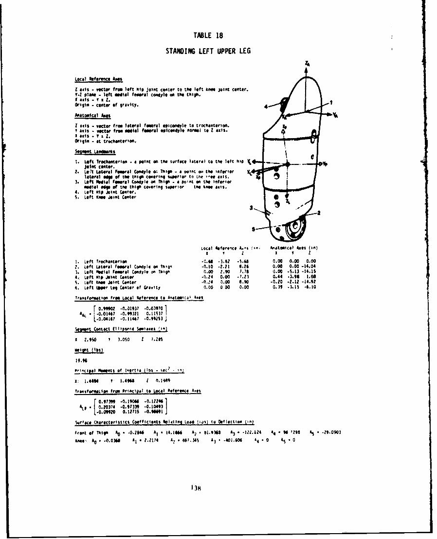
TABLE 18
STANDING LEFT UPPER LEG
Local eference Axes
Z axis -vecto from left hip joint c~enter to the left OEM" joint center.V- plan left mdial femetal condjlo an the thigh.I ails - I X Z.Origin - Center of gravity. 4
Anatoical Axes u
Z ails - vector fro lateral femoral eeicodyle to trocantlllron.V aIls - vector from mdlal femral *plcoadjla, normal to Z ails.Sailts - T 2.
Origin . at trochanterlfi.
1. Left Trochanterton . I int on tro ivrface lateral to the left hip YIq ..
Jets? Center.2. Le'?t Lateral Femal Covitte w.. Thugs . a point oo the inferior k
lateral i of the thigh Covering suwerior to ne i-ef atil.3. Left lla ramrl Co.,lel on Thigh . a pont n the Inferior
megial s p of te thigh covering superior the knee axis.4. Left HIp Joint Center.5. Left One Joint Center
13 I
Local Reftfi'e L i nt Anitomical Ales (ift)I f I I I I
I. Left Trochanterlon -C.44 .3.62 .S." 0.00 0.00 0.00?. Left Lateral Fameral Conoale on Thiqg -4.10 .Z.1 6.26 0.00 0.00 -14.043. Left MIa116l femral Condyle on T1ign 0.00 2.910 1.8 0.00 -. 13 -14.154., Left HIP jo110it Cntr -0.2t 0.00 -7.21 0.44 .3.96 1.08S. Lieft Knee int Center .0.-4 1.00 6.0 -0.10 -2.12 -14.924. Left Upper Leg Center of Gravity 0.00 0 00 0.00 0.39 -3.1S -6.10
tansformatton from Local Reference to Anatomicl Axes
r 014 -0 .03,,04 AL -0.0160 -0. "32 0.1is0 ,
L-0.04167 .0. 1147 -0.99al4
st"nt Contact (lit0vid esliasei lia)
I 2.9S0 I 3.080 1 1.48S
wigft (iIs)
19.96
Pi-. pal momestl of Inertia -11 *. 'CC
1: 1.4494 1 1.4944 L 0.1989
Yranformaklon from Prlnci~al to LocAl efelren As#%
. [ 0.973 9 .0.1044 -. 0.241A I 0.203)4 .0.9y339 -0.104693
-0.09920 0.12IS .0.9 I I
5urface Characteristic$ Coefficients 401tlij Load tios) to OffleCtio" [ta)
front of thigh Al • .0.Z844 Al - 14d.16 A? 8 01.934 A, - -1.'624 A4 Z '$ At, 41-9.0903
Knee A0 • .0.0)4 A, - 1.1114 A?, 61.34S A3 .. 401.40 44 0 As 0
13H
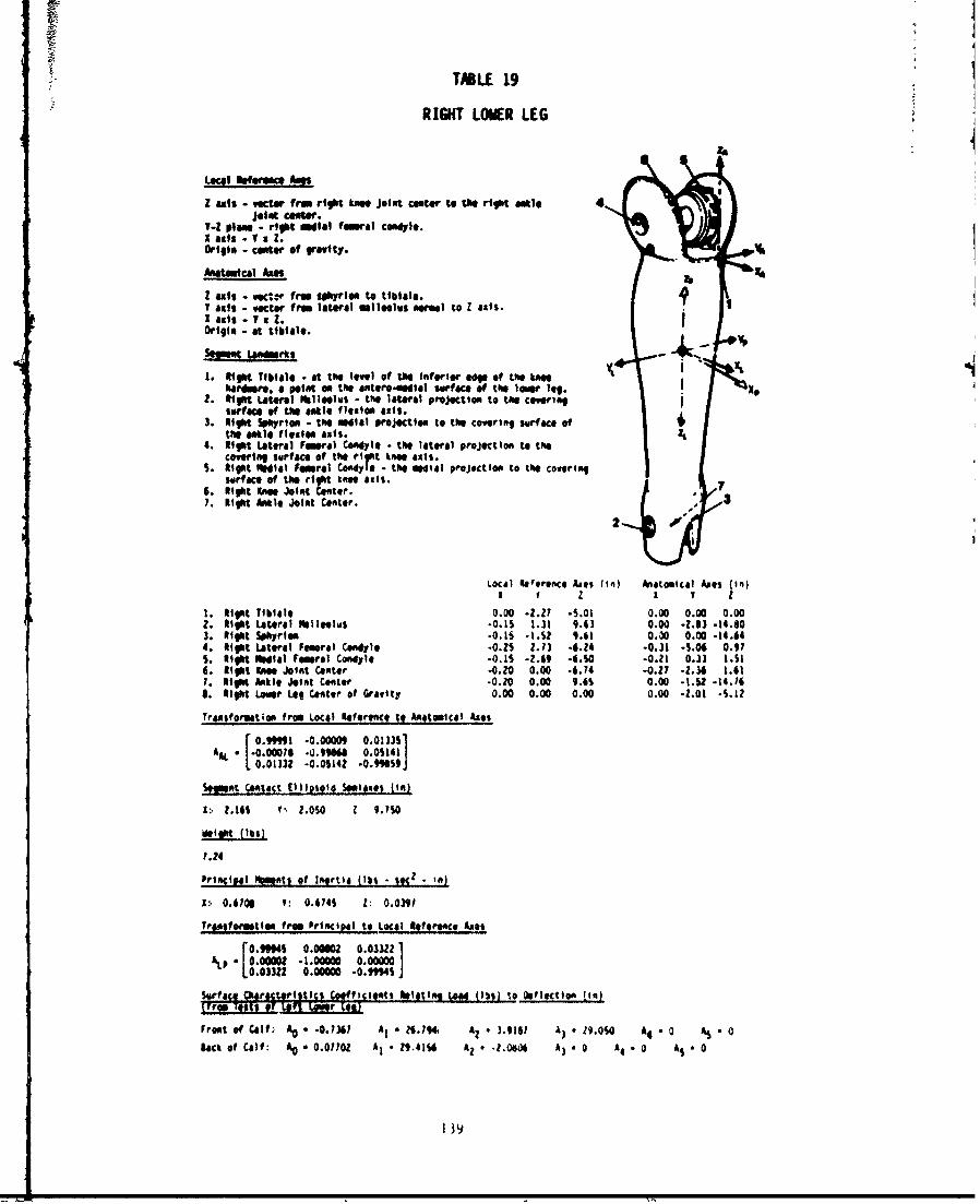
TMLE 19
RIGHT LOWER LEG
Loca lterasce AMe
Z "Is - "er from rigt knee joint canter to te riot ile 4joint Costar.
9-Z plan - right anial feinal comile.I axis o I a Z.Origin - center of gravity.
Anatomical Ame
Z axis -vgc:r from sfytrio to tbille. 41 .V axis - vector from lateral illelws noral to Z axis.I ais -x Z.Origin - at tibiale.
1. lot Tiblile -at the level of the infiter " of the ee Iharlre, a point on the antero-odial surface of the loew leg. IX
2. Right Lateal sblloolvs - the lateral projection to the coveingsurfacm of time ankle flexion axis.
3. Riot Sphyrtem - the iniill Projection to the covering surface ofthe sale flexile axis.
4. Right Lateral Femoral Coadyi - the lateral projection to tmecovering surface of the rigt knae axis.
S. Rigt 110i0l F Cirta C -|i the meotal projection to the coveringsurfKe of the right knee Sat.
6. light Koe Joint Celter. 31. Riot Ankl. Joint Center. 3 -
Local Reference Axet Inl Anaetoecal Ails (in)I I I Y I
I. light Tibiale 0.00 -2.27 -S.01 0.00 0.00 0.002. aight Lateral PIllels -O.1's 1.31 9.63 0.00 -2.3 -14.803. Rigt Sphyriemt -0.15 -1.62 9.61 0.0 0.00 -14.644. Rigt Lateral Femoral Condyle -0.?S 2.13 -6.24 -0.31 -S.06 0.97S. Right tial reeral Conayle -0.1S -4.69 -4.50 -0.21 0.33 I.5l6. ligt Knee Joint Center .0.Z0 0.00 -6.14 -0.27 -. 36 1.411. light Ankle Joint Canter -0.20 0.00 9.6S 0.00 -1.32 -14.16S. Rigt Lower Leg Ceter of Gravity 0.00 0.00 0.00 0.00 -2.01 -.11
Transformation fire Local Reference to Antotcal A&es
*0~S .. 94 .540.99991 .0.00009 0.013311AAL -. 00076 -0.190i 0 .05 41/1 0.0132 -0.0142 .0.99G9 J
Semnt Contact Ellipsoid Sase (i)
V 1.16% ZOSO 9.1s0
Meilht (1hi)
7. 24
Principal !lMnts of Inertia (l1% - s .c2 -
i:, 0.6706 1: 0.ts45 1: 0.0391
Tr!Sforatllon I,, Principal to Local Reference A* t
[O.0.941 0.00M0 .0.033221AL, ."m000 -1.00000 0.00000
L0.0332 0.00000 .0.94S
STts~ L (Its tor Ioflectioo if)
frost of Calf., Al .0.1361 A, Z.I Az *.t-14 A) • 19.0w A4 0 AS 0
ack of C4lf: A 0 .0.010Z A, 9,41% A, -1.0606 A 3 0 A4 •0 As 0
119
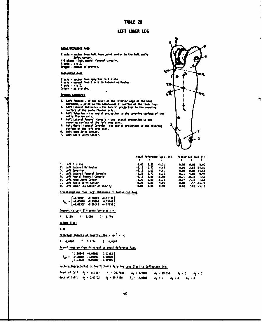
TMLE 20
LEFT LOKR LEG
LOCal Noferam lam
z ads - stee frm left "a mat cow to the ft 1@bl
Y-1 Om - left -sa I towel c=Ibe.I ads - V a L."08 .- cow of r yt.
z adi - facto fromn sollyrs to tthlale., oslo - mousi frmr 2 as to lateral veit. us.
OkIgi - at tiblale.
1. Left liblele - at the level of the fer-tar OW of tM 1111110bwm . 0point am the atoro-aetal sorfac of tM low-lg
2. Left Lateral ftlsaolus -the ltel projection to tocow mlgsrfa of the eat1e flovion ealt.
3. Left sparion - the swt inr-jetiotoa the co"aorl serface of toeeabto Flexion eas.
4. Left Lateral Fmrai Comey the towel "rJectlem to thecover-log our-fac of tfe left knee axis.
5. Left htfal Fomoal C4019 - the adiat projeCtlem to the CMO§-asurface of the left kaen at%.
4. Left am o t ha Conter.I. Left Anale Joint Coater. -
Loca I Neoeaco Age$ life) bfatical Amges (In)I I I I I I
1. Left Toblale 0.00 2.2? .S.01 0.00 0.00 0.002. Left Laterael hel loolies *0.1s .1.31 9.63 0.00 2.83 .14.603. Left 5ehyr-se -0.1s 1.32 9.61 0.00 0.00 -14.44. Left Lateral roweal Coni 1 e -0.25 -2.73 4.24 -0.31 5.06 0.97S. Left bOtel Fier-l Ceoslo -0.1s 2.04 4G.50 0.21 -0.33 1.516 . Left "oa Joist Cealer -0.20 0.00 .4.74 .0.21 2.34 1.417. Left Amele Joist Coater -0.20 0.00 9.6s 0.00 1.52 -14.76I. Left Lawer La Coaler of &@*Slty 0.00 0.00 0.00 0.00 2.01 -S.12
Tra~sformttom free Local leferwact to Anatomical An"S
004.991 .0.006 .0.01iJ5 1AM. * 0.00019 -0.96W .0 0142 114.0133M 00.0§142 .g)961 m
1: 2.145 1 ,2.0O50 Z' 9.750
ifoif ( 05)
7.24
Frisctoel Slowt of lar-t1e (lbs . Soc2 . in)
1:0.6701 1., 0.4144 1., 0.0397
iro-,. 'maom fror Ortacitel to Lfill bfROWSK&ie
mm 0.94 0.00003 0.03322nALP 0 0000 -10 .099945
Surfect LsarfcIfrl$1fc 1 S..tflclOet1 UOltlai jleaf Ij to 0fl1iO40 [is)
Frotof Calf 40.-.136? A 346 Al J.111 Ate2*.MOO £4.0 A5.0Wecof Calf, A %007g A(.?i.415 A .2-0"6 Al3.0 A4.0 £S.0
140
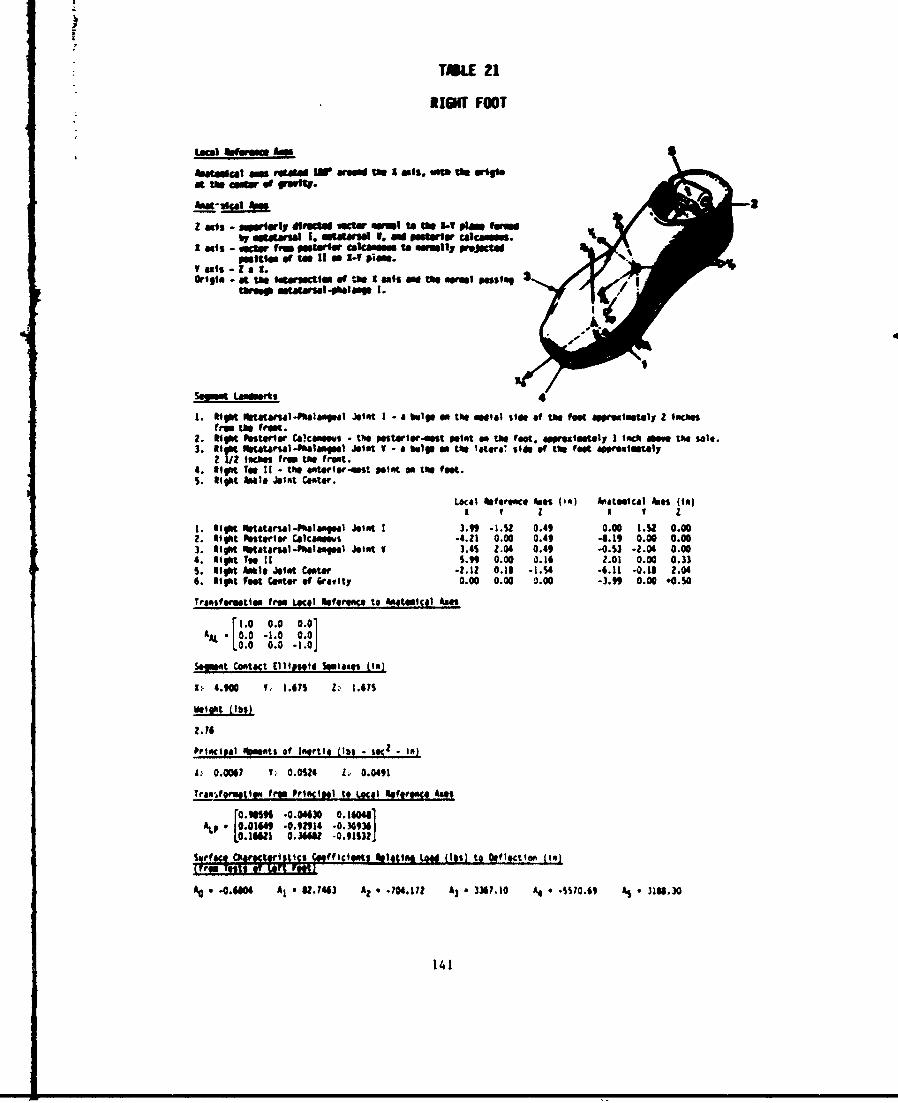
TAKE 21
21IHT FOOT
RpowCal tam ao wu oda st.a i il
at- tw me f2W
Z I ads~f 1, dfwlrly N vctm NMI to 0s 9-1 PIM ftnuI "U"MaIa 1. UniiOr V. a UM otr Cako vsm
I axis - VKW I Mfr gelo~ tolaeM "I "eMily wrM "thpngm of t It as -1 pis".
IF oxis Z 2 1 .IGrie a f s ltoa es of a* I St " ust aw l postl 3
1. 111Kt Jtt lDiaag o int I -a beie on the aia) side of tfe foot agpromintely 2 tech"sfrom the front.
2. INht Peitome CGICaneMMS - the wetorloe-mest Msetts the fast, o! v Imlue I Inch aboe the sale.3. Rioht fttrul-baluagel ist IF - a lp a tie 'atera sid of tow feet affeuleetoiy
2 1/? Inches from us f ront.4. 11i1"t Tee 11 time eatorler-aWst peint eN the feet.5. lvgt Apale Joint CatoW.
Local Reerence Axes 0("'I Anaomical toes (101)A I z A I I
I. :ihttot etrsu.Iloag~ Jeint 1 3.919 -2.32 0.49 0.00 1.M 0.002. 1 9git Pestorlee Calcaneews -4.21 0.00 0.49 4.19 0.00 0.003. 1ig1t firtatrsl-pial"Wgee Jeowl V 3.45 2.04 0.49 -.3.3 -2.04 0.004. klgkt Tee 11 S.99 0.00 0.16 2.01 0.00 0.33S. Nllgt Apile Jeint Costa. -2.1? 0.11 -.. 4 -6.11 -0.11 ?.046. Rioht Feet Costa. ef 6.evity 0.00 0.00 0.00 -. "9 0.00 .0.50
Tras*feruetem f rom Local mefereec to a~teeC~l An@%
ro0.0 0.0 1
00 0.0 .2.0
Salwt Catict (lioseld SuuiameS (in)
X: 4.9M00 1. .7S 1:, 1.67S
weight ohbs)
Priocipal Oieents of Inqri (la %K .~ .n
A, 0.0067 COW 1-,* 2 0.0491
Tram-.fqetou. from Prl#cisel te Iecol %sfqr**4e LAos
OSS 96 -0.04430 0.16084At 0.01649 -0.9fl14 .0.34936
10.16611 0.364u .0:91S31
AO -0.6104 Al * 61.7413 A2 e -M0.172 £3 * 1331.10 A4 * _S510.69 AS* 31$8. 30
141
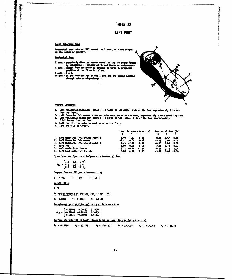
TXLE 22
LEFT FOOT
Looffoiw ft" iIV*g agfitas
a ta we -o of rarity.2
or immelaul 1. "atwsl V. ad Ogstew calcinm.it MIS - leter from Pa.51mM calcamins to e rinl1 110401183d
PWIVtt' 66 taOIt1so -1 pan.V gMIS - 2 a L i.
W tin - a 11e o rsatl m p t OSa o tm .4
1. Left Mttaisl-0alanggal Joint I - a 66191 - tagile al Sideof tag feot aolostgly 2 tlosfre twt front.
2. Left Posterior Culcamous -tog ogttoret Point on the (OgK* ppzimtgl I lack Ame tag [email protected]. Left Iltarfl.F la"ga Joist V - a mulp on tag lateral sid of the fasteo alesutely
2 /P foc"Sfrm f rot4. Left Too It - the aatfloe-at pglqt so the feot.S. Left Wel Joist gsattr.
Local fogam Ames 11o) &towicul Agin (14)I I I I T Z
I. Left littoral-fhalonsgl Joint I 3.99 l.S2 0.49 0.00 -1.$Z 0.002. Left Posterior Calcbagous -4.21 0.00 0.49 .3.19 0.00 0.003. Left ~ttraJmlaolJoint I L.is .2.04 0.49 -0.S3 2.04 0.004. Left Tog II S.99 0.00 0.16 2.01 0. 1 0.33S. Left Aftl* Joist Ceomer 42.12 -0.18 -1.34 -4.11 0.13 2.046. Left feet Cgntgr of Gravity 0.00 0.00 0.00 -3."9 0.00 '0.10
Tra.,ftyrigtinn fro Local Reftrec. to miatgimmcaI Age
rA 1.0 0. 0 0.0. 0 .0 -1.0 0.0L0.0 0.0 . 1.0j
sesew Contact (IIIgsld Slmlgg ORs)
1: 4.900 1: . 1 AS I 1.67S
"Itht fibs)
2.74
pr~ncteI IWts of Inoltia (1% - Wc2
9: 0.0061 1-. 0.0124 1, 0.0491
Tr2Rsfwptl! es . Pwi~cips to Local Seformnco Ages
r0.96"m 0.0"630 0.1048A*ps -0.01649 -0.92914 0.36
[10. 1421 -0. 362 .0.91032]
lien-f 0 K nteistics Coeficlogis Agti~jLa il"ts l" u. fl
AO -0.6M0 A1, 2 1463 A? - 4104.112 A, o )My. 40 4 _SS10.69 Aj 3 118.30
142
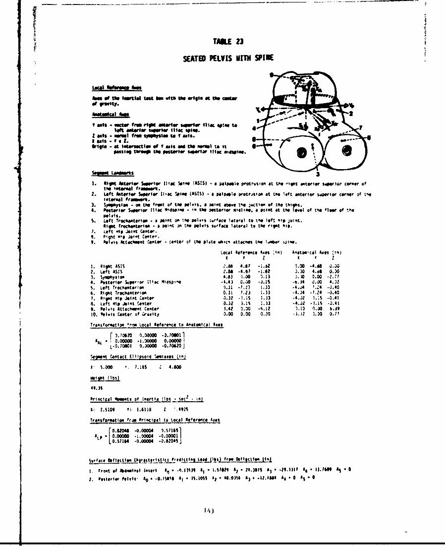
TAKE 23
SEATED PELVIS WITH SPIKE
amo f me OWtlal tat us wits tw 0191M a tft comteof frortty.
I ants - vemir Ir ript sertue sowler mt~ sepau ta -
LMft moaifr O W or iliac [email protected] ats asOmni fewr~IS ~gto I &MIS.I &IS - I a .Oriffe - at Iatersoctis of T "is ame tw oearl to It
1110111101 t*rw tft "5ter W"Oelar Iliac masles.
I. Riot Asteor soertgv Iliac spine MS) - a palpasIt protrusion at tft rilat anterior gupertce corner ofthe latafeal frintort.
2. Left Aptentor hoprior Iliac stia. (4525) -a palvaelop protrJsIoe at the 'oft anterior S'Arior corfer of t"101termal V rrOfw.
3. Sy~ta - ae utn. froat of the pelvis. a point aaevo t%@ joctiwrn of t".oigs4. Posterior Sgperior lilac 001dstie - i the postortor sitting. a point at the level of tE% f*1g of toai
S. Left Trocheantirn a point on the polvis ;wr'act lateral to taig left nIV joinit.Right nirchiantorion a po'ht a the pelvis surface lateral to the right hip.
7. Left Pelp joint Center.e. *isst "to Joilit ct-te'.9. Pelits Attacmnt Center - Center of the p~ito %ic% dttacfts the laftr s~imo.
Local Reference Ajes tin 4 hte~a A) ~ i
I I I a I I1. Right £515 11.8a 4.87 *1.SZ 1.00 -4.414 J. 30?2. Left ASIS Z.68 .4.67 -1.62 3. )0 4.68 0.301 . sympys Ian 4.53 1).00 M.3 ).)0 0.00 -.. 174. Posterior Soperior Iliac 0111i 'he .1.43 0.30 -'3.1', .14 J. 00 4.)2S. Left TroChaniftgrfae 1.31 -. Z2 1.33 -4.,A '.14 -.3.406. Right TrocXia0twtt 0.31 Y.23 1.33 ..3 *1.Z4 -0.407. Night "it JoIint Lesiter -3.3z -1.45 1.33 .4.j2 1.3 .0.41S. Left Htip Joint Center 0.32 J. I% :. 31 .4.32 -. ISj -3.419. Pelvis Attaclh" Center 3.42 0.30 -4.12 ).1) 2.30 6.3910. Pelvis Center of curavity 0.00 0.00 0.30 -.. 3 2.30 0.77
Transformation tra Local Seforefce to Anatomical Ame
1.706Z0 0.3,000 -3.706011ANA 0.0000.1.000M0 0.000001
Segmot rontoct Ellpso#4'i .asos Ltn)
11 S.000 I. 7.3s5 4.8ON0
Pvifaciaul %mvots of inertia 001i - tz
I:. MIN0 1:. 1.6110 1 .1492S
tronsforumation fra Prinicipal to Local leterence AAg,
I 0 .8 0 4 -0 .0 0 0 0 4 1 .5 1 8 5 1*t 0.00000 .1.00004 -0.30001I
10.S1164 -0.00004 -0.80045j
Surface kflqctil*4 0 ttiii viffgic tloei..ilbs #too Oftle fie) 1
l1. o O~if ffIMli 10$0 1 *0P A ll A , -6.1056 A , -400 14 3 .18 A) £ 4 *M 0
vqltqrw 0#10- AO *-0.1S~l A, - ISA 43-4.M A 1.46 4 0A
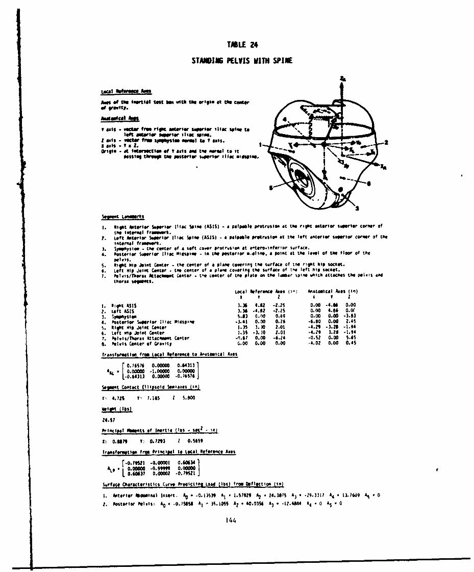
TMLE 24
STANDING PELVIS WITH SPINE
Local Ileftro As
Amr; of th Imert~oal test oft III tf o* rigin at tft coattrof rV"Ity.
T as - vft2 fr M111 orior suttirliI ait to %left mmIthilligrior ,liac spie.
Z oats - weem trim s~stm asemI to 1, aNIS.
Grlle at lstorsectiem ef V axis ai the "WWIa to ItPassing thrIs- 0 the porstoer wome Ifg IJac esilspino.
1. RItht Atorior Saperior iliac Spine (ASIS) - a palpable ptru1o at tme right anteror swperior corner oftihe internal framewrk.
i.Lft loterior Saperfor IlIac Soino (ASIS) - a valpablO protrusion at time left anterior superior corner of thlei1ternal V roinee.
3. SynI -~s time Center Of & Soft cover protryigo it attrO.inftr!0r Serf IeA. Posterior Suerior Iliac 11iospime - to the posterior s.ollno. a point at the level of tme floor of Et
pelvis.S. Right Nip jint Caer ie comter of a pilane coverinq the suirface of tnot right sip socket.6. Left tip joint Center .the centor of a plant covering tile surface of t'me left nip sociot.7. Plvis/Thera: Atacnms Cnter . to* center of time plat* ani the lumar spint watich attaches the pelvis aid
tisoras soomt5.
Local Aeortimci Aes (j. Anatomical Ann$ (in)I I I I I I
1. light Ashs 3.36 4.82 .25 0.00 -4.46 0.002. Loft ASIS ).36 -4.02 -2.25 0.00 4.86 0.0(3. systoiysiom 5.83 0.00 0.69 0.00 0.00 .3.834. Posterior Soprior Iliac ifidsiss -3.41 0.00 0.26 -6.80 0.00 2.45S. Rittt 141P Joint Canter 1.:15 310 2.03 -4.29 3.28 -1.946. Lift Hip Joint Ceniter 1.31, .3.30 2.01 *4.Z9 3.26 -1.947. lielfis/Thoras Attacmet Cantor J1.61 0.00 -.64 .0.S2 0.00 9.65S. Pelvis Coster of Gravity 6.00 0.00 0.00 -4.02 0.00 0.4s
Transformatlas from Local Referenc to Aatomicl Aes
Fo. 76576 0.00000 0.643131
[-,e10.64313 0.000 .017
Seamt Costact IlliPsOid $oo'aas lin)]
V 4.729 1, 7.189 1 5.800
weit (l0s)
principal 1%mmos of -inertia (IDS sac wiz in)
1: 0.U9 Y:, 0.d293 Z 0.S651,
trasfouptosfrom Principe) to LQ~aI_ Re4fe e Axes
r-."1.0.00001 0.50341
Su.rf ace Charcteristits Eirve Predicting4 Load (lbS) frog flt io (in]
1. Anterior 411401Wl Insert. %0 e 013 A, * 1.97129 A2 # 24.341S A3 -29.111 A4 1.1609 AS 0
2. Posterior Pelvis:, A0 # .0.75898 A, 35.1099 A2 - 40.0354 A) a -11.4W8 A4 * 0 AS 0
144
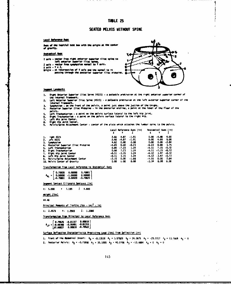
TMLE 25
SEATED PELVIS WITHOUT SPIKE
Local ftfwiw paem
pnof t"e Imortial test b" aft% as 0"90 at the Maur
0ISMS 1011011
I axis - wettor f" em t a~ener Suerior Slla spin toloft Uateri efsormI I iac estee
Z ad~s - wedti free ""WP~IM beft to V ali.6 .
" ais *VaL
Grille at tuterimem ef V so$ ada tft WeWI to itpasin to"eu the Poseior superIer iliac alasete.
1. RiKMt erier %Wer lia&c Spine !(MIS) - a palpabwo protrusleex at to* rttpt anterlor buaerlor corner ofthe lateral tfrunert.
2. Loft Warertr Superior Iliac Spine (MSIS) -a Palpatle protruihs' at too loft u..trior Superior corner of :ihetnurnal I romert.
3. syslem - so the front of too peltis, a Point just aevo tie juctioft C# tine talips.4. posterior Super Iliac 149911 . fi too posterior slting, a poist at the lootl of the fleer of the
pelvis.S. Left Tracearion - a peoit an the pelvis soaface lateral to toe left lip jo'nt.: int Trclntorlem . a peint so the pelvis surface lateral to the rillit Nip.
a. at MNip jont Cenaw.9. Pglvls/SPln* attacmet Cnter . center of tfe plate 101co attach"o toe lwar SPIRE to tue pelvis.
Local Reference Lot 014) An'atomical Axes (in)
I. I r StIS 2.4 4.87 -1.91 0.00 .4.86 0.002. #ft MSIS Z.44 .4.87 .1.91 0.00 4.13 0.003. Syosiam 4.62 0.00 0.00 0.00 0.00 -044. Posterior SupeIor Iliac Pidiplat .4.6s 0. 00 .0.23 -5.20 0.00 3.75S. Left Trec11antorien9 0.00 ..2 1.24 -4.11 ?.IS -0.72S. allot Trechantorlon 0.00 1.23 1.24 -4.11 -7.15 -0.727. Iirt Nip Jotint Catr -0.11 -3.1s 1.24 -4.12 3.97 -0.726. Loft NIP Joint Conter .0.11 )AS 12.24 -4.12 -3.97 .*7!9. Pelvts/$Plno tac1118 Ceittr -2.1s 0.00 -1.66 .SS1 0.00 2.6410. Pelvis Coster of Gravity 0.00 U-00 0.00 .3.34 0.00 0.30
Transformation from kocal fOfermoe t AnatomIcal WuS
IA 0.00M -1.00000 .0 0000.o70Mg 0.00M00-.762
Sam!' rotact (111osold Selasks (In)
I:, S.000 1 7.10S 1 4.00
44.4'
Pris~clps' Nonts of 'artlo (lbs . S"t 2 . in)
1.. 1.016 :, I.m1 1: L.2060
Trsusforelo frpe Pricip to WSJal Reference Axes
.r 6.192 -0.011017 11."M 1,AL 14.0001 .0.99992 *0.01)t
140.0062 0.0010 4.19112 J$,,rf1 2'filci" Cu.rctrtl o Prelcil L@6 ls) from Dflection tin)
1. Front of the 1604 Insert:, A. e013 A, 1.572 42 * 4.3671 A3 *-21.3317 14 13.74.09 AS~ 0
2. ftster',or Polvis: A0 *-0.51M A, - 35.1011 A2 40,0114 A3 *-12.404 A4 & 0 AS 0
145
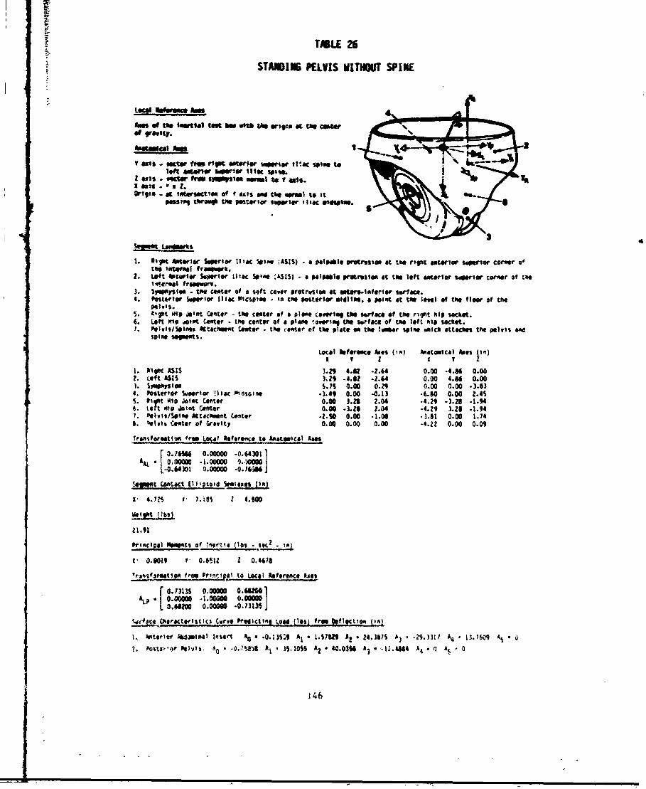
TALE 26
STANDING PELVIS WITHOUT SPINtE
Loeal Item hom
As of the ItMial tast Samn thu m-igu K t" Cester
of yv't . N.
bt~A~t l PRO$
1 a215 - IK Iftqp rtpt aeor bow or iliac %pipe toloft 401,4029 5StAW r lIVac SOSiw
Z es octo fmw srumplwa "In to y 0$5.S axi's - w a 1.Ort9to - if ipf tasom4 of t "f$ a the eaguel to It
OMs0te twoN l t posterior wit e, lilac .sdus".
!4
I. 11K 4~16C Uperlor %lilac 51e 'ASIS) - a Palble "rtrestn at te ript anterio soperior corner a$tihe latrfal| frafrt.
2. Left a09Wcter Superior iltac Seite ISIS) - a palpable pracrlslom at to* left estrlor u prior corner of thetcroal rimprt.
. 5i)q"Mstqa . the center of a soft cover protrisloa at altersIntferlr surfaca.4. Pstetor suetr l1iK Pclsle - itn te posterior oldlime. a point at tow leel of the floor of the
S. CtIPt Hip joint Ceter - the center of a plane Cewerlag tie sorface of the right RIp socket.6. Left Nip joint tenter - the center of a plae overls the sorf*.e of tae left hip socket.7. Pevts/sti~s U ttcoft Cater - the rafter of ta, plate e the lmr sellne , cJ attacies tee pelvis a
spine segts.
LocI ?ftion A00% (In Anitomical ns In)
1. Allot £115 3.Z9 4.82 -2.64 0.00 -4.86 0.002. Left £52S 3.29 -4.62 -2.64 0.00 4.84 0.00). Smlslom S.YS 0.00 0.29 0.00 0.00 -3.834. posterior Superior -Iltc p'esone .).49 0.00 -0.13 -6.80 0.00 2.4S5 at I p jotot Center 0.00 3.28 2.04 -4.29 -3.28 -1.946: Leot Nip Jotet Unter 0.00 -3.20 2.04 -4.9 3.26 -1.947. Pelvi/slne Attachet Ceter *?.SO 0.00 -1.08 -3.81 0.00 1.74
S. eils Canter of Gravity 0.00 0.00 0.00 -4.22 0.00 0.09
Transformation from tLOa leference to Anatomical Les
0.71"" 0.000M0 .0.64301AL -. 64 30 0.00000 -4.16AGI
~sqg: contact (111psold SeuSave (in)
1, 4.2 $ W" 7.I1 1 4.800
21.91
1. 0.9019 1. 0.011 1 0.40,8
vrtsforlmtvA_ fre Princ, to Locl Reference Aset
[071S 0.000M G.682oALP •o.OMoo -I.M= o.0M
L .8820 0.0000 0.7313S
%sege Charterlstlcs Curve PrOCcttns Load (l)61 fu!p 01flctio (10)
1 wtiitf Ablo1tA4 1,er * *0.1)1.9 A, 1,1718 2 1,1 4.811 £, 1~.9J)I11 A4 370 A! *
t riw.s r polts., 6i0 .. MASS. A|, A3.10SS A? 40.031 A, i 4l661 4 At. , &, 0
,46
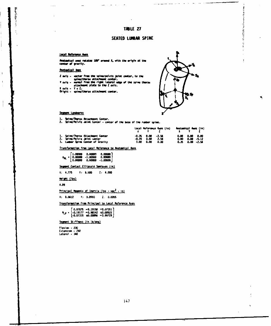
V4
TMLE 27
SEATED LIDISM SPIKE
Local bftrc. pa
bAtscuiea tsm 1V stood 1. Wi th C00 wis) at tfQ~e of Vanity.
4vtodcal amt
Z ants - MWte frm Lb somwtooplvt. joit t sw.. to O
av t " is NM frm thm tI1 laterl sop of t"sofaue tweaxattacbeat plaoe to t" I ash~. (
OHIMt - liptsa/tbeas attcmm coalegor.
2. $pieus/Pelvis Joint teeter - ceetor of tm@ "aso ot th. r~*s Sol*&.
Loco) lletrom Anng (fit) Amutesocal Ann (1.)A I I a v I
3.solmel/rewae Atuichst C~so -0.3s 0.00 -2.56 0.00 0.00 0.002. Spit/Pelvis Joint teeter -0.35 0.00 2.56 0.00 0.00 -S.12I. U~AW Spine Caser of Gravity 0.00 0.00 0.00 O.AS 0.00 -. 54
TrfevugStles free LK41? agftea to fAlili) ANes
.3.00000 0.00O.10000
Sotst contact Lilfteld lemsaaes (10)
1: 4.77s .: #.SOO Z:, 4.000
Proncogal ftme s of Inijibs pg 5
1, 0.06)? T., 0.0%93 1. 0.020
Tramsfomutia. free Pvigncll to Local lof rvocoo Axes
[9675 -0.191W -0.0135111:0:.19117 -0.96142 40.0052*
1:1*3540.006 -0.99119
Sepst &tffnsss (fIs lb/IM)
F11004" - 31Extension - 250Latoral .340
147
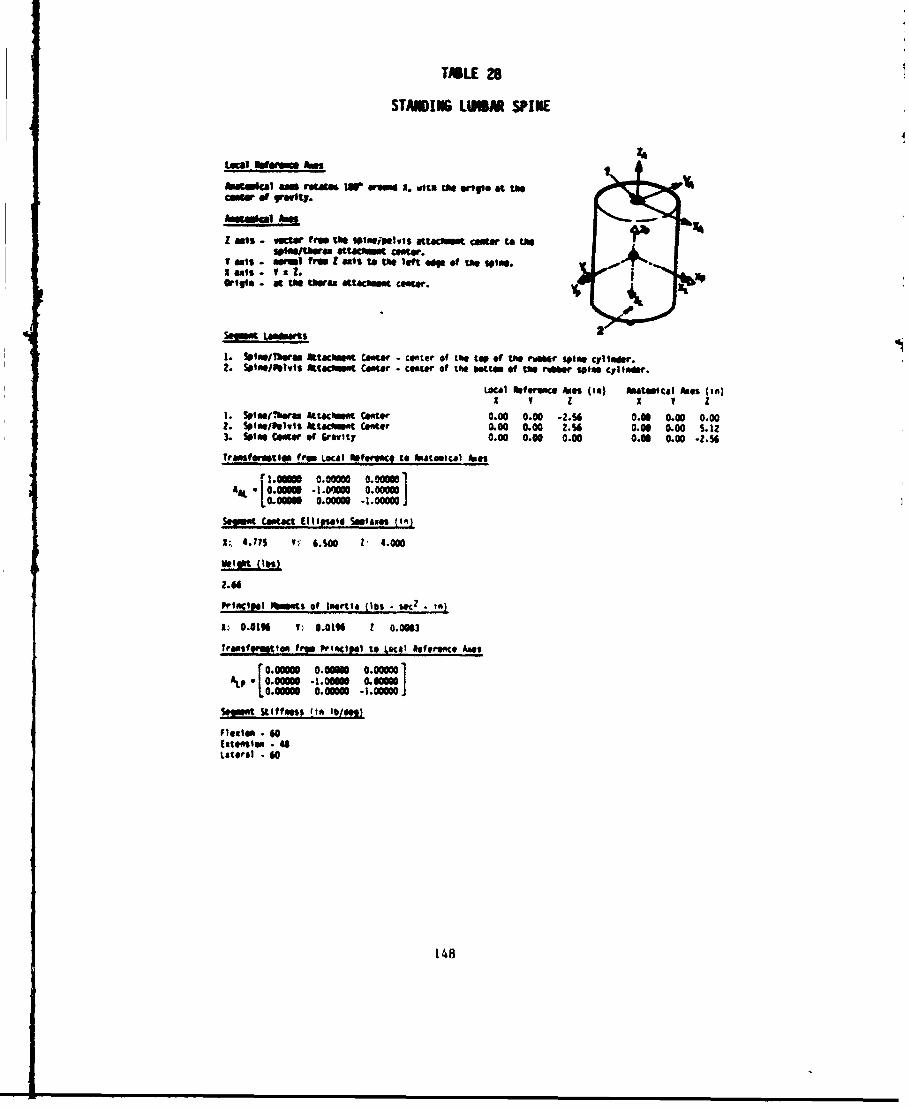
TABLE 28
STANDING LIM SPINE
:4
I axis - @am fromsI all tio he left e ofte at ee
I xs - I Z N2rgl a t. mthe fiwr t e 6fltS atnc. XLt t
1.sisb" ita ao ct Cose-atr o ~ o fter o"clerV e/t Aot tachmeunt tam ti loattmo of te botosfte.. tfsim ylw
I. btu./Th-wron Attachent Cs. eter 0o0 0.0 t2.W 0o0 tie 0.00 1 Cl~it
2. SI..(ttfteaa Attacleet Cator 0.00 0.00 -2.S4 0.00 0.00 0.003. Sploo Center of Gravity' 0.00 0.00 0.00 0.00 0.00 -2.56
ttaforsntton f ro Local eferorg to Omitomical #Ae
rAL ' 6olw oo0 0.00000
1.60 0.00000 .1.00000J
Slow Contact Ellipusoid S &$as tin)
I., 4.7 I-, *.Soo 1. 4.000
Pvtamclgol ft.sns Of Inertia (IDS - SW2 .in)
U: 0.0196 VY. 0.0196 z 0.0093
Trentsferutlo from PrIOCIeni to Local Refernwe Amos
ALF, .0000= 0 1.00O 0.00000D10.00000 0.00000 .1.00000.
Sevelt Stiffness (to 111/6111)
116.10p . "0
Citotlem - 48
Latoral - 60
148
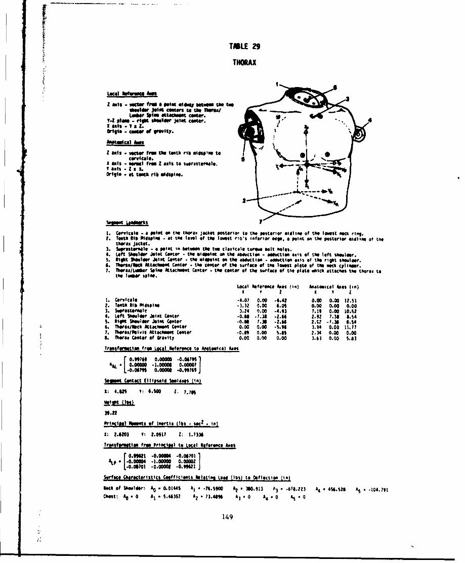
TELE 29
THORAX
Local Usa A Mols
1 axis Vaese ftme a poa slow "two &aheauisldai Joist centars to ton Tharaa
Latr Sofa attocum cowte.Y-Z p1IS, - riot souldr Join caowe.I axis T X 1 .orlt - coiw of puIty.
Amasalcal Ams
2 ais - Vector from the tenth rib uidspins tocarvcale.
Soatis - NMIt from Z AIS to suprosteM.ra.V axis 2 Z X LOrigim - at tenth rib midspins.
1. Cervical* - a point an the thorax Jacket posterior to the posterior miii ins of the lowest meca ring.2. Tet% Rib 011splia -at the level of the lowst rio*s inferior ege. a point on the posterior eidI ins of tne
thorax jacket.3. Supastarmle - a point in bet""a the two ClaviCale torque bolt holes.a. Left ShoUlder Joint Center .the midpoint 06 the 66ductIon - adductiant ats of the left Shoulder.S. 1ligt Vioher Jint Center .the oldpoint on the abution - adutlon ants of the rigot shoulWe.6. Thmra/l~ck Attacmt Centor - the center of the surface of the loast plate of the neck cylonss.7. 1hera/Lar Spins Attachment Center .the Center of the surf ace of the. Plato which attaches the thorax to
the le~ Spins.
Local Reference Anes (in) Anatmical Axes (in)I V z I V I
1. Cervical@ .4.07 0.00 .6.42 0.00) 0.00 12.512. Tenth 116 101spins .1.32 0.00 6.0s 0.00 0.00 0.003. supralteflle 3.24 0.00 .4.93 7.19 0.00 10.324. Left $Moulder Joint Center -0.64 .7.38 -2.64 2.92 1.38 8154S. ligh Shoulder Jeint Canter -0.81 7.36 -2.66 23;2 -7.34 846. Thosa/dueck Mtacmeet Center 0.00 0.00 ."9 3.94 0.00 11.777. Theax/Pelvis £ttachmWn Cantor .0."9 0.00 1.I5 Z. 34 0.00 0.00S. TWAra Canter of 6ravity 0.00 0. 00 0.00 3.63 0.00 6.83
Transfarmatian fram Local let erence to Anaomical As*%
r0.9976 0.00=0 .0.0679SA * - 0.00000 .1.00000 0.00001 1
L 4.06791 0.00=00 .99769 1
%plont Contact Illipseld Seats [lot)
1: 4.8n V., 63100 1.
39.22
Principal !MtS of Ionta (lbs . 5gcz town)
1: 2.6203 1: 1.0517 L: 1.1136
Tr4AnfjMetIoN frI Weincipa to Local eferonce ages
ALP - O .0.0000 2 .0.9921LW .0.001 1Sqrface QChateristics Coefficients OWIatina le## (155) -to 0eflectios (in
back of shoulder. A0 0.0144S A, a -?6.1900 A2 e N60.913 A3 , .618.223 A4 *4%.S28 A5 .- 104. 791Chest, A eQ At .4057 A , 1.4#% A 3*0 A4 *0 AS *0
149
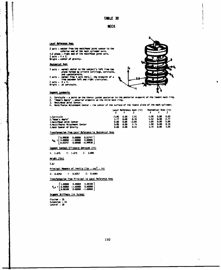
TMLE 30
NECK
Z ats -vector free teO jecaio oint caeor to toeinferor ON of tie mock cyllr mi.
-z plan - rst a of te nocl/hed jint axs.Z ats - T a Z.Oriole . cancer of gravity. 40.
Amtmcal ANNs
V ais - W Il vector to the s*Ject's left free tooplanIIfIefm IV crtcelo cartilage. cervitcale.
I ats - nrml frig V its sinro" the stepont of aflow betile left ad ritt clawiCoes.
Z smts - i 1a .Oriole - at cervical*.
1. Cirvical* . a point s to@ tawos jacket posterior to the posterto eatotnt of the loiwt mook ring.2. "is d ple" - anterior elpoint o too third netS ring.3. flck/mea Joint Center.A. aoKk/ThoPa ttiatrmnt Ceter -ao coor of the surface of too lost plate of toe sook cyliner.
Ltocl Seforoace Ann (in) Anatmical Aes (It)
l.Corvtcale -. 8s 0.00 2.91 0.00 0.00 0.00."Ad's Aplo 1.11 0.00 0.36 S.92 0.00 2.7
].*ca/"d Joist center 0.00 .00 -2.4 3.69 0.00 $.894.opcti/TVoe AttockOe Coster 0.00 0.00 Z.?6 i." 0.00 0.305.Oeck center of Gravity 0.00 0.00 0.00 3.14 0.00 3.09
Transfoertta from Local ftefersce to antomical Ates
.9 0.00000 0.0374?A*L 9[ 00.0000 -1.00000 0.00000
0.03741 0.000O0 -0.9930 J
Segot Comtact Ellesimd Sas'aaes (Is)
X:, 1.61$ ; 167 Z. 3.000
ett (lbs)
?.61
Principal PemtS of Inrtia (Ibs . scZ - n
: 0.024 Y. 0.029? Z, 0.0004
TransfM tss free Principal to Local ieferelce Axes
4LP .0.0004-.000004 .00
[' 0.00100 0.mo .1.00000
1Son Stiffness tie Iwdool
fil4ssion. ISfloteslo - IS
Lateral - 30
150
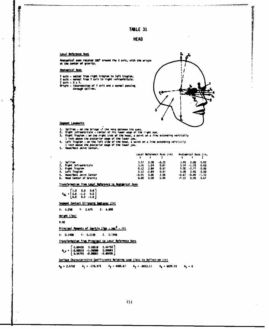
TBLE 31
HEAD
l Wforom , Ames ,
MIC4e4Chl ams eiltd In0 $roed the I axis. with te originat te cMesr r gealty"
Amiamical Am
V a"is -vetor fro riot tragion to left tragloo.I axs - wal ftrms V axis to right lefrahltale.2 axis - A x V.Origin .intectw of V axis a m a morml psing
through 50111a.
1. Stlle" - am the brdo (J) the note between the eyet.2. Illt ;Aframittals . center of tb2 low ed ge of the rigt e"o.3. tMot Tragion . O so ten right sie of the Roa. 4 point on a lira eate ding vertlcally
I Inch Sao the 0stoerl"or ad of the loop jaw.4. LIft Trllon -on t1 l1ft side of te r.od, a pomt A a iem extming vortltlly
I inch ae the posterior top of the Ioter jaw.S. fad/heck Joint Canto?.
Local efe'om' S (4) Aatomical Ants tinoI V Z I v t
1. Soeli o 3.57 0.00 -0.15 3.45 0.00 0.922. llot Iafrao"Itall ).ZS 1.04 0.6? 3.14 .1.10 0.003. Mogt Trgloem 0.12 Z.64 0.61 0.00 -?.71 0.004. Left troglm .1 .2.84 0.61 0.00 Z.90 0.00S. hadWd/hck Joint Center -O.S 0.00 2.00 -0.67 -0.00 *l.336. iM Center of Gravity 0.00 0.00 0.00 -P.12 0.00 0.61
Traofeorat io from Weil ftesifce to Anoocal A"
AA 1.0 0.:0 0.6:0.0 0.0 -1.0
Segmet Cotct Ehh Iissot wss tin)
1: 4.0 1: 2.07% V 4.000
wa~l (160)
9.92
P incipal Imt of taws (1 . ie?. In)
X: 0.140 1: .2IN I. 0.1916
Tr, n,,fo tlem fr PrIo il to ,ocal loroaco Ams[O.oa, o.00010 0.441SO1
A~p .0010 1.00066 0.0"S690o. 4% $ 0.0061 .0.6 .
Sowfage Characteristics C.ffc ;tnt$ fleltlo Lou (Ilt) to 1*tloctioe ($n)
AO e 2.742 Al e .176.917 A2 44.67 A3 * -895.t At 609.59 A5. 0
151
2.2 (IS/AU Model Simulations
2.2.1 Conversion of Basic Data to (IS/ATB Model Format
The A7B model characterizes the body as a set of rigid segments linked
together by joints. The seveiteen segments and sixteen joints chosen to
describe the Hybrid III body are listed in Table 32. Also in the Table
is the chaining scheme in which joint J connects segments. j + I and
JIOT(j), Wlere JNT is an input parameter.
Two AI data sets have been developed; one using the seated manikin and
the second using the standing manikin. The data sets are identical
except for the lower torso, middle torso and upper leg segments and
pelvis, waist, hip and knee joints. The tables in the following
sections contain the seated manikin's data. and the standing manikin's
data for thuse segments or joints are included at the bottom of each
table. Where data were not available from this study, the data from the
Part 572 dumy data set developed by Calpan (8 were used. The
complete, formatted input files for both manikins are listed in the
Appevidix.
2.2.1.1 Segment Characteristics
The ATB model requires the weight and the three principal moments of
inertia for each segment. The orientation of the principal axes is also
required and is specified in terms of yaw. pitch, and roll rotations
from the segment local coordinate system. These rotation angles are
obtained from the direction tosine matrix for the transformation from
the principal to local referenc* axes. Table 33 contains the mass
properties for each segment and the principal axes yaw. pitch and roll
angles.
152
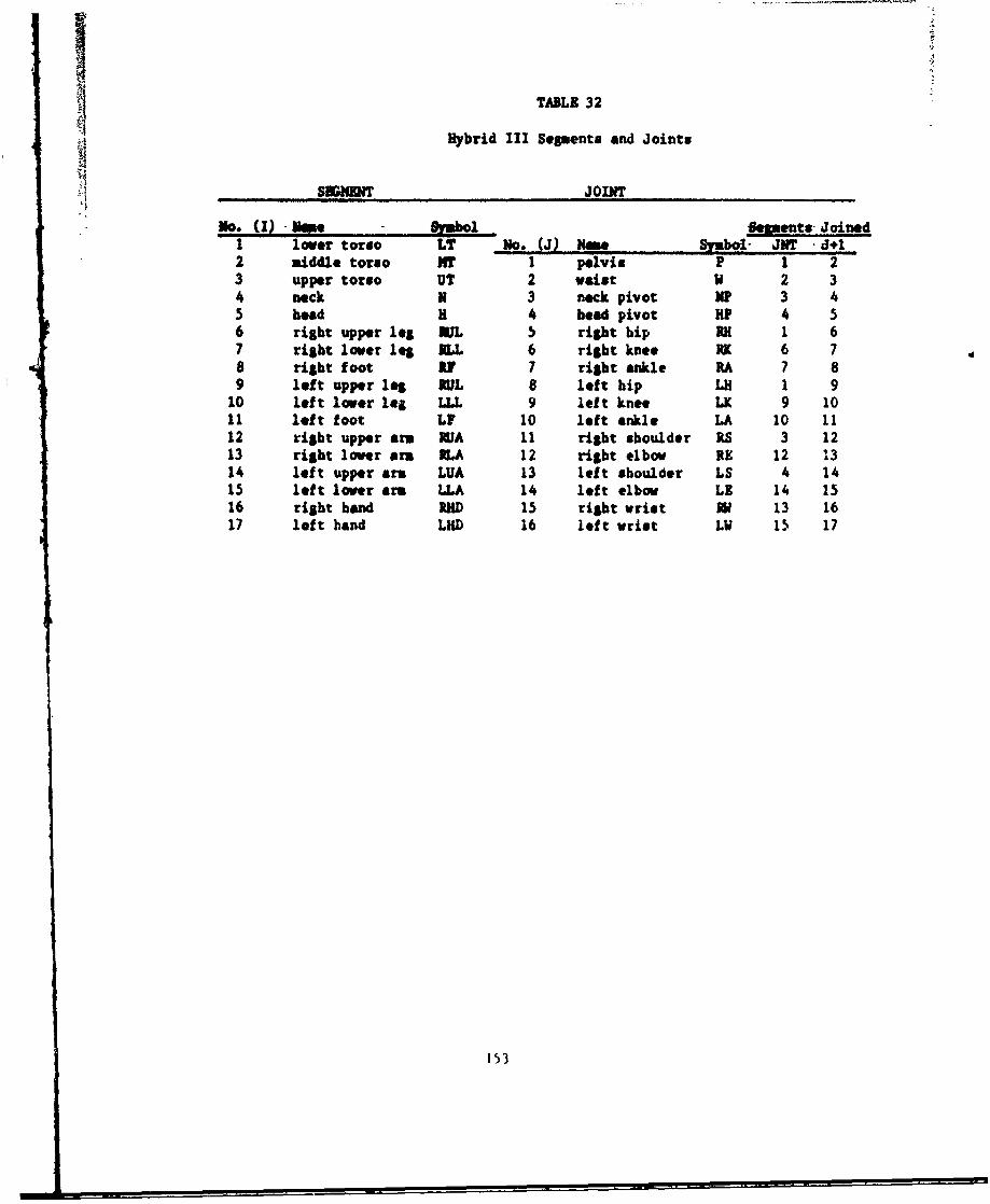
TABLE 32
Hybrid III Sepents and Joints
SKHRIT JOINT
No. (,) awe _eSm, s- Joined1 lower torso LT No. (J) Now .Mb- JNT d+I2 middle torso MT I pelvis P 1 23 upper torso UT 2 waist W 2 34 neck N 3 neck pivot NP 3 45 bead H 4 bead pivot HP 4 56 right upper le NIL 5 right hip Rl 1 67 right lower leg ALL 6 right knee RK 6 78 right foot IF 7 risht ankle RA 7 89 left upper le RUL 8 left hip LH 1 9
10 left lower le LLL 9 left knee LK 9 1011 left foot LF 10 left ankle LA 10 1112 right upper am NA 11 right shoulder RS 3 1213 right lower am ILA 12 right elbow RE 12 1314 left upper arm LUA 13 left shoulder LS 4 1415 left lover arm LLA 14 left elbow LE 14 1516 right hand RED 15 right wrist Nu 13 1617 left hand LHD 16 left wrist LW 15 17
153
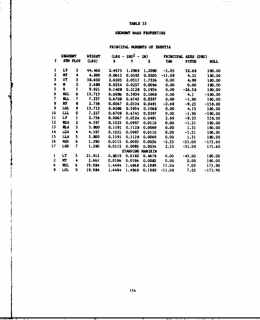
TABLE 33
SEGENT MASS PROPER~TIES
PRINCIPAL MOKiNTS OF INERTIA
SONUT WEIGHT (LBS - SEC2 - IN) PRINCIPAL AXES (DG)I SIM PLOT (LBS) X y Z YAM PITCH ROLL
1 LT 5 44.460 2.4575 1.2969 1.2080 -1.05 52.68 180.002 XT 4 4.890 0.0612 0.0593 0.0205 -11.08 4.22 180.003 UT 3 38.630 2.6203 2.0517 1.7336 0.00 4.99 180.004 N 2 2.680 0.0254 0.0257 0.0084 0.00 0.00 180.005 H 1 9.921 0.1408 0.2128 0.1956 0.00 -26.58 180.006 RUL 6 13.713 0.608b 0.5934 0.1068 0.00 4.1 -180.007 ILL 7 7.237 0.6708 0.6745 0.0397 0.00 -1.90 180.008 Ri 8 2.756 0.0067 0.0524 0.0491 -2.69 -9.23 -158.009 LUL 9 13.713 0.6086 0.5934 0.1068 0.00 4.13 180.00
10 LLL 0 7.237 0.6708 0.6745 0.0397 0.00 -1.90 -180.0011 LF 1 2.756 0.0067 0.0524 0.0491 2.69 -9.23 158.0012 RUA 2 4.597 0.1025 0.0997 0.0110 0.00 -1.31 180.0013 ILA 3 3.800 0.1191 0.1128 0.0069 0.00 1.31 180.0014 L.UA 4 4.597 0.1025 0.0997 0.0110 0.00 -1.31 180.0015 LLA 5 3.800 0.1191 0.1128 0.0069 0.00 1.31 180.0016 RHD 6 1.290 0.0115 0.0093 0.0036 -2.35 -31.09 -175.6017 LUD 7 1.290 0.0115 0.0093 0.0036 2.35 -31.09 175.60
STANDING MANIKIN1 LT 5 21.912 0.8019 0.6182 0.4678 0.00 -43.00 180.002 MT 4 2.661 0.0196 0.0196 0.0083 0.00 0.00 180.006 MJL 6 19.984 1.4494 1.4968 0.1989 11.0b% 7.03 173.909 LUL 9 19.984 1.4494 1.4968 0.1989 -11.08 7.03 -173.90
154
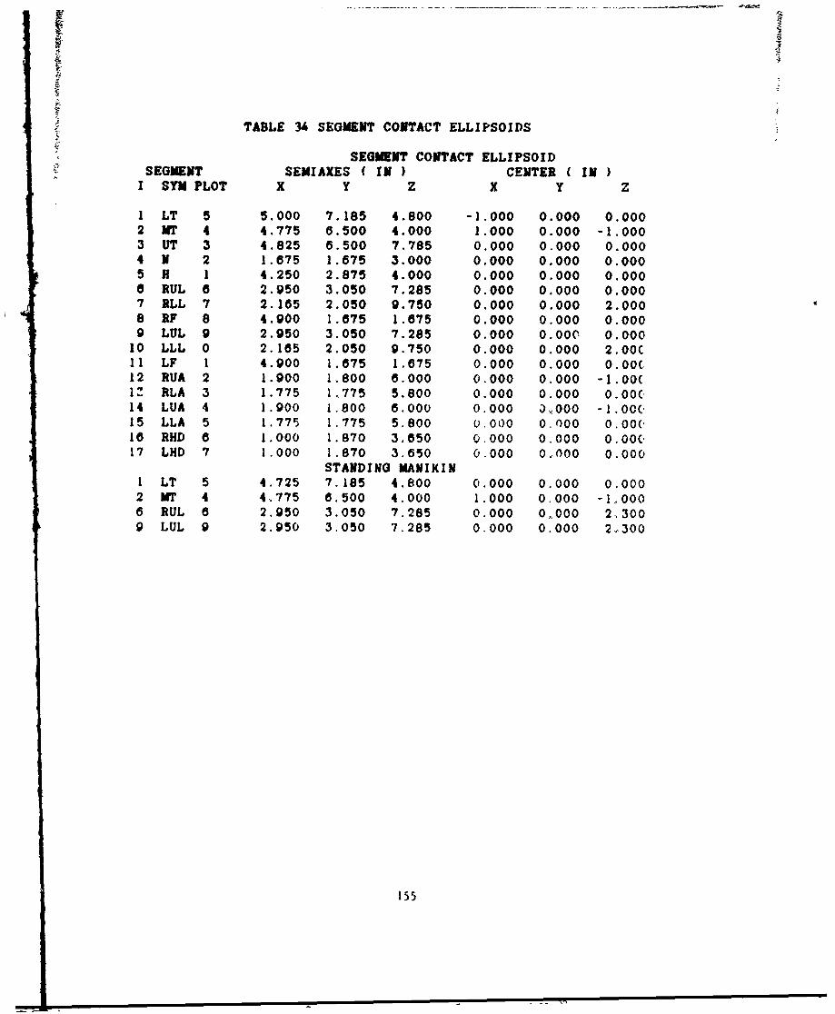
TABLE 34 SEGMENT CONTACT ELLIPSOIDS
SEGMENT CONTACT ELLIPSOIDSEGMENT SEMIAXES ( IN ) CENTER C IN )
I SYM PLOT X Y Z X Y Z
I LT 5 5.000 7.185 4.800 -1.000 0.000 0.0002 MT 4 4.775 6.500 4.000 1.000 0.000 -1.0003 UT 3 4.825 6.500 7.785 0.000 0.000 0.0004 N 2 1.875 1.875 3.000 0.000 0.000 0.0005 H 1 4.250 2.875 4.000 0.000 0.000 0.0006 RUL 6 2.950 3.050 7.285 0.000 0.000 0.0007 RLL 7 2.165 2.050 9.750 0.000 0.000 2.0008 RF 8 4.900 1.875 1.675 0.000 0.000 0.0009 LUL 9 2.950 3.050 7.285 0.000 0.000 0.000
10 LLL 0 2.185 2.050 9.750 0.000 0.000 2.00C11 LF 1 4.900 1.875 1.875 0.000 0.000 0.00(12 RUA 2 1.900 1.800 6.000 0.000 0.000 -1.00(1Z RLA 3 1.775 1.775 5.800 0.000 0.000 0.00(14 LUA 4 1.900 1.800 6.000 0.000 D1000 -1.00(.15 LLA 5 1.775 1.775 5.800 0.000 0.000 0.00(l16 RHD 0 1.000 1.870 3,850 0.000 0.000 0.00c17 LHD 7 1.000 1.870 3.650 0.000 0.,000 0.000
STANDING MANIKINI LT 5 4.725 7.185 4.800 0.000 0.000 0.0002 MT 4 4,775 6.500 4.000 1.000 0.000 -1,0006 RUL 8 2.950 3.050 7.285 0.000 0,000 2,3009 LUL 9 2.950 3.050 7.285 0.000 0.000 2,.,300
155
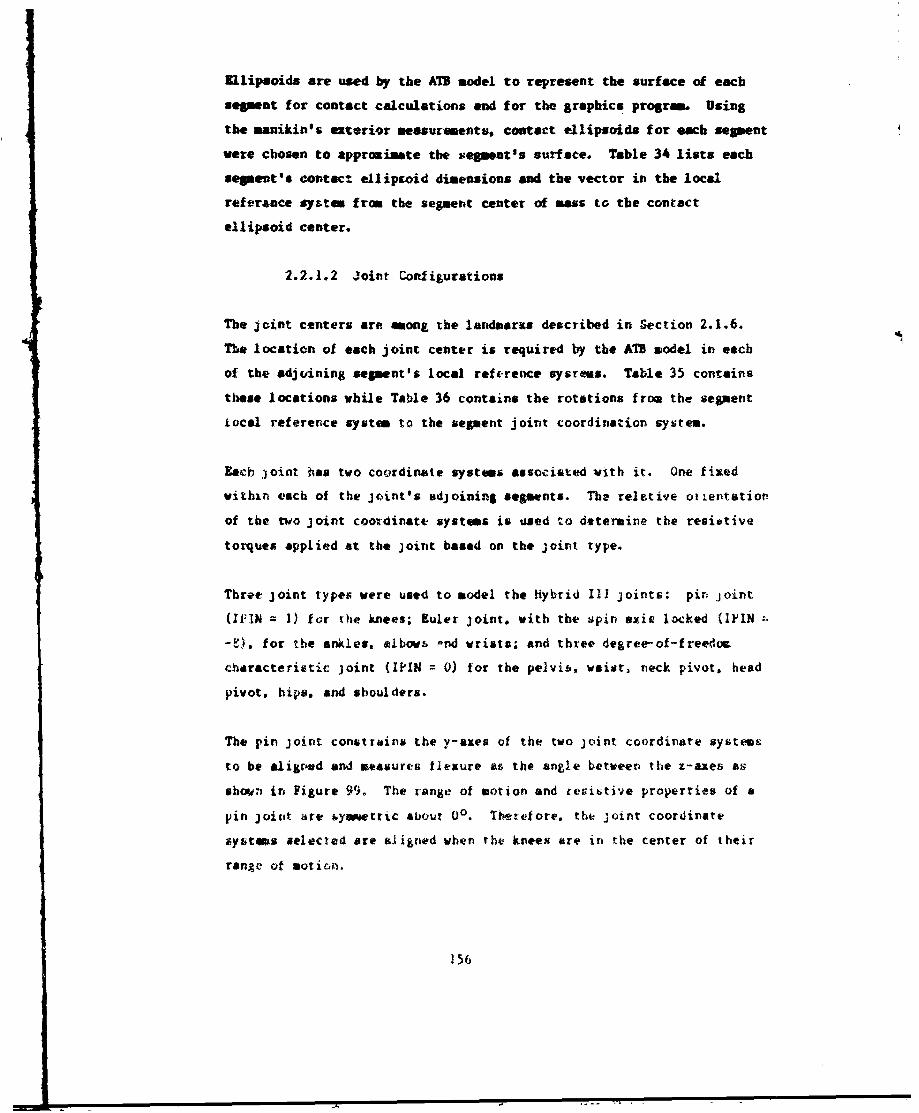
Ellipsoids are used by the ATE model to represent the surface of each
segment for contact calculations and f or the graphics program. Using
the manikins exterigr mesuroments. contact ellipsoids for each segment
were chosen to approuiuzate the scegmnt's surf1ace. Table 34 lists each
segpmt's contact elliptoid dimensions and toe vector in the local
ref erance system from the segment center of mass tco the contact
ellipsoid center.
2.2.1.2 J~oint Conf igurations
Tbe joint centers are emong the landmaris described in Section 2.1.6.
The location of each joint center is required by the ATB model in each
of the adjuining segment's local reference sysress. Table 35 contains
these locations while Table 36 contaIns the rotations from the segment
Local reference system to the segment joint coordination system.
Eacb,)oint has two coordinate systems associated vith it. One fixed
withxn each of the joint's adjoining segments. The reletive otetation
of the two joint coordinatte systems is uased to dettermine the resittive
torques applied at the joint based on the joint type.
Throt, joint types, were used to model the Hybrid III joints: pin, joint
(IVN =1) for the knees. Euler joint, with the spiAn axir locked (iPIN
-E), for the ankles. elbowb -nd wrists. and three degree-of-freedoL
chdracteristic joint (IPIN = ) for the pelvib, waist, neck pivot. head
pivot, hip. and shoulders.
The pin joint constrains the y-axes of the two joint coordinate systest
to be alig~d and measures flexure as the angle between the z-axes as
shown in Figure 99., The range of motion and revibtive properties of a
pin joitit are iyaoetric about 00. Therefore. the joint coordinate
sybtws selected are sligned when the knees are in the center of their
range of mot xon,
156
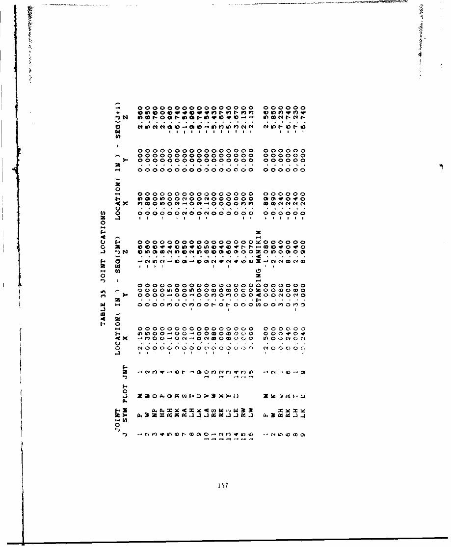
-0000000000000000 000000
ow C1- o -ov)C4C4 0 0 "t- t-
0000000000000000 0000000000000000000000 000000
>4 0000000000000000 00000 0
0000 C0C; 0 0000OOO0 0 000000
00000000000000000 000000
0 m0o0c0" oc"0oooo ~oiov wo4 X MOOMON0-001-OO00V MdI' O ~4# 4 C* C
Cl) 0 000000"400e000000 000000a .3 . I I0
24
U E 00o000o000o0000OX000o0o
4 ',OMNOWN00000Z00Ofl000O-~ ~~~~ .. .- 4......
-00 0 0 CiNC)NOz 9d0-( 0
>4 ~ 00O0-00-00"'O"~000400N'I0C
w ~ 00000~0M Zo-oOO-000wo "Ono
4 a1- 0
140000000000000000 000cloo1-4 IA I 0 0- 0 0 -'0 0OC Q 0 0O0O IV0w4 X -"00-0" O w oro (n~0~i ~0 C14 0(4
0 N0000n C400O C 00'C0 a C1 0 C'4,C
Z~~~~ ~ -C4lq -lt ..4 0 - 4
0.4 a 0 C*.am 0 > S 1 X % 1 1 f
4
0
-Cir)~~ ~ *$ot 00 -N VO C4 U- toOD(
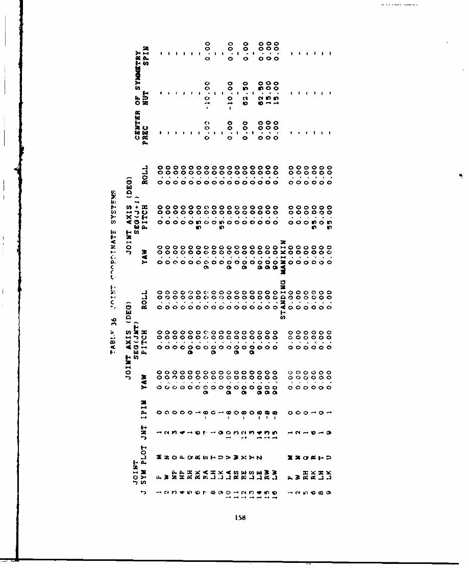
0 0 0 00020 0 0 000~~4I.4~~ 61 11 .6 6 . I I166#
04000 0 0 000
0 0 0 000
0) 0 0 000
0 0 0 000
A~ 0000000000000000 000000.3 0000000000000000 000000 4
F-M+ 0000000000000000 000000
5)- CI) 0000000000000000 000000
z, 0-'~ 0000000000000000-0000003f 40-. 0000W00W00000000 000U000
Z 3 0 00000000O00000001-'000000C. 4> I I . . . . . . . . .
W. 00000000000000004000000
%00
Is Wt= 000000c,000000000'4000000-I~.4 0000000000000000 000000
C - 0 . . . . . .4c 40" c OoooO 0ooOOOO CoOo4000000
F w C6 t At t
0i 0000000~000000000 000000- 3 4O0r0000C000000000 000000
44-~ . . . . . . . . .>*4.- 0000000000000000 000000
Op a~ 0 0 0 c
0 4 000000M000000000 000-00
44 ..
C4 0000v0 i1- 0- 0 0 -C0 e 4 I0 -O0i) 0 CID
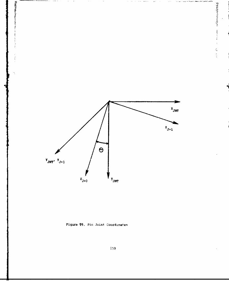
J+ I
YJNT Y3+1
Figure 99. Pin J.o Coordinates
The Wat joint. wirh the spin axis locked, constrains the rotetion
between the JUT joint coordinate system to the J*l joint coordinatesyste to be a s tbination of two body fixed rotations. first is a
precession rotation through angle 0 about the z-ahix; second is a
nutation rotation tbrough amgle S about the ew x-axis as shown in
Tigur* 100. Separate ranges of motion and resistive properties are
defined for each of these rotations. As with the pin joint, these
characteristics are symmetric, but the center of symmetry can be defined
a input. The centers of symetry used for the anles. elbows, and
wrists are in-luded in Table 37.
The three degree-of-fretdom characteristic joint requires the joint
coordinate systms to be aligned in an equilibrium position, with the
z-axis of the JkT& jzint coordinate system as the torsion axis.
2.2.1.3 Joint Rotation Rsistive Torques
The jcint resistive properties ore prescribe4 in a number of different
ways depending on the joisit type. For the pin joints used to model the
kn es, four parameters (linear, quadratic and cubic spring coefficients
and joint stop) are required to define the relationship beeen torque
and flexure. 0. The angle 0 ii measured from the equilibrium position
in which the two joint coordinate systems are aligned. Figure 101 shows
how these paremeters are used to dWfine th& torque. The curve is
symmotric about 0 = 0. therefore flexion and extension must have the
sae stop characteristics. A typical cuive from the joint tebting is
shown in Figure 102. The center of the range of notion was chosen as
the equiiibriu position end the free tango of motion determined the
oint stop angle, 0s as that angle at which the resistive torque
increases in a nonlinear sanner with incre-sing angle of rotation. The
linear spring coefficient. C. was set to zero to model the free range of
motion. The remaining two coofficients prescribed the soft stop.
Initially. thik resixtive range of the soft stop was digitized and a
least squarez method vas used to solve for the quadratic and cubic
coetficient6. Althouh thib method fit the data well. some
160
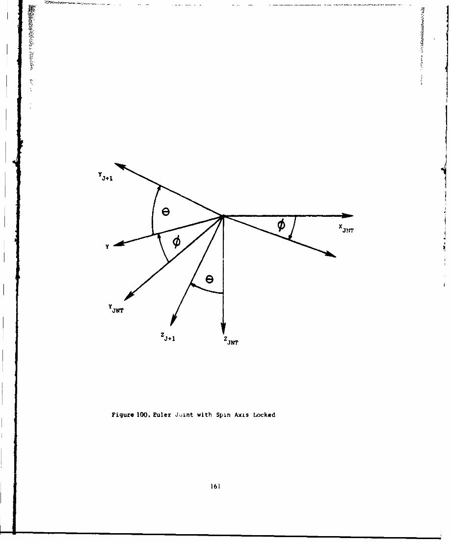
y
y JNT
Figure 100. Euler Joint with Spin Axis Locked
161
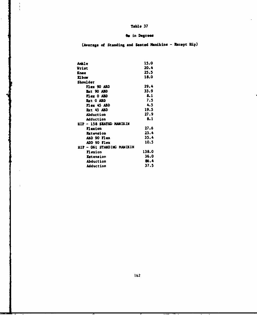
Table 37
On in Degrees
(Average of Standing and Seated Manikins - Except Hip)
Ankle 15.0Vrist 20.4Knee 25.5Elbow 18.0Shoulder
flex 90 ABD 29.4It9O AD 33.9Flex 0 A&D 8.1st 0 ADD 7.5lex 45 AD 4.5
Ext 45 ADD 19.5Abduction 27.9Adduction 8.1
HIP - 158 SLATe MANIKINFlezion 27.6xt eneion 23.4
ABD 90 Flex 35.4ADD 90 Flex 10.5
HIP - 061 STANDING HANIKINFlexion 138.0Extension 36.0Abduction 86.4Adduction 37.5
162
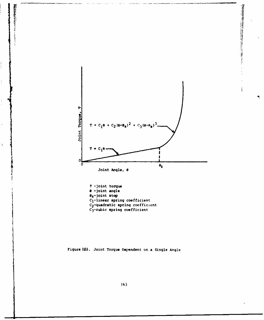
S T -C10 + C2(e-es)2 C30+
4
0
T CIO
00
Joint Angle, 0
T -joint torque* -joint angleB8-joint stopCl-linear spring coefficientC2-quadratic spring coefficientC3-cubic spring coefficient
Figure 101. Joint Torque Dependent on a Single Angle
163
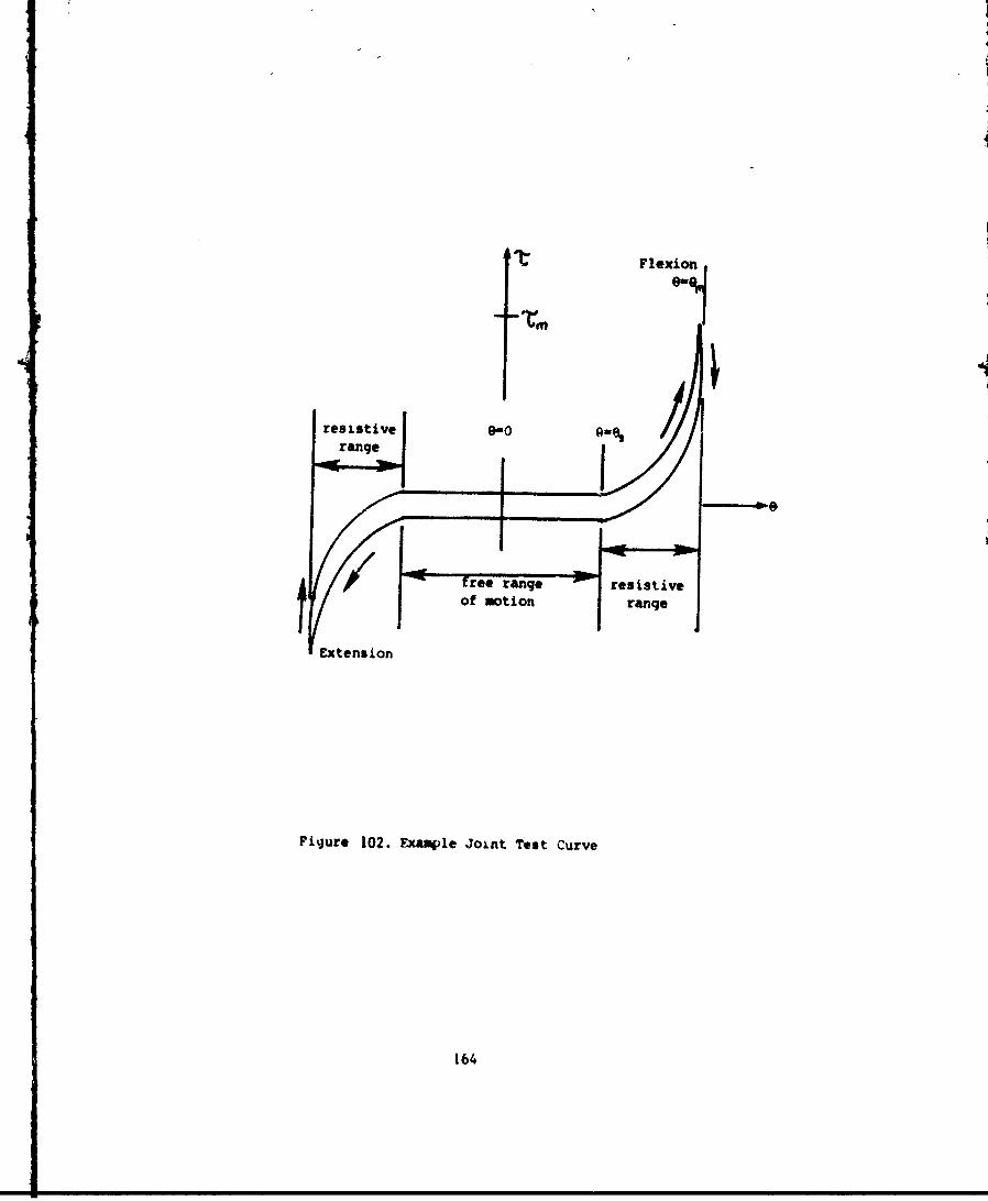
Flexion
resistive Gin0 /-range
r/free range resistiveof motion range
Extension
Figure 102. Example joint Test Curve
164
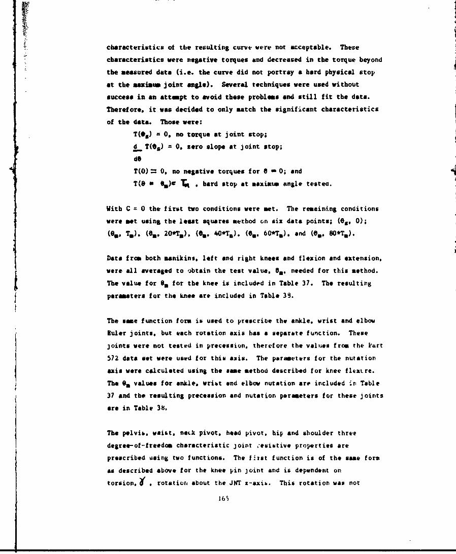
characteristics of the resulting curve were not acceptable. These
characteristics were negative torques and decreased in the torque beyond
the measured date (i.e. the curve did not portray a hard physical stop
at the maxism joint angle). Several techniques were used without
success in an attempt to avoid these problems and still fit the data.
Therefore, it was decided to only match the significant characteristics
of the data. Those were:
T(*s ) = 0. no torque at joint stop;
i. T(Os) = 0. zero slope at joint stop;
dO
T(O) 0 0. no negative torques for 0 0 0; and
T(O % )w %% . bard stop at maximum angle testes.
With C = 0 the first two conditions were met. The remaining conditions
were met using the least squares method on six data points; (0g. 0);
(9a. TO). (0a. 20%~). (e8. 40eTm). (So. 60*Ta). and (ea. 80*T1m).
Date from both manikins, left and right knees and flexion and extension.
were all averaged to ,obtain the test value. 0 ., needed for this method.
The value for Oa for the knee is included in Table 37. The resulting
parameters for the knee are included in Table 39.
The same function form is used to prescribe the ankle, wrist and elbow
Ruler joints, but each rotation axis has a separate function. These
joints were not tested in precession, therefore the valoies from the Part
572 data set were used for this axis. The parameters for the nutation
axis were calculated using the same method described for knee flhxtre.
The m. values for ankle, wribt and elbow nutation are included in Table
37 and the resulting precession and nutation parameters for these joints
are in Table 38.
The pelvis, waist, neck pivot, head pivot, hip and shoulder three
degree-of-freedom characteristic joint -esibtive properties are
prescribed using two functions. The first function is of the same form
as described above for the knee pin joint and is dependent on
torsion, * rotatioai about the JNT z-axib. This rotation was not
16
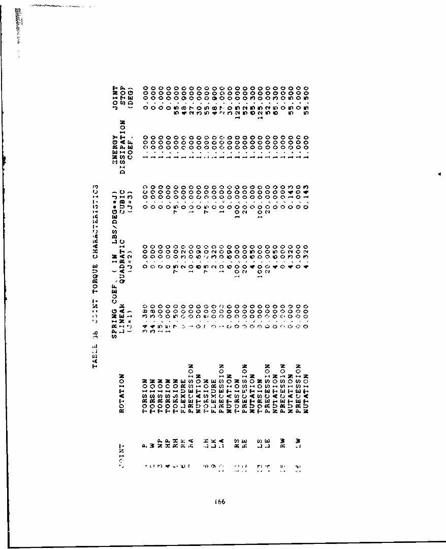
1-04 - 0O0OO0OO0O00O00OOOOOO0000 0oo0o0ooo00o0oo0000oo0
-4w OO0 00000000000"00"0000l~
0
OOQOOQOOOOC'000000000000o0414 0000000000000000000000%A~w 000000000000000000000O
V) 40 1.
0000 000000000000000'0"o"-0- 0 UC000O0000O00OOO0000v0v-) " rI) 000 00 O00000000O-0
0~ *: OO OA ii,00000000000 0 0 0 0 0
f-4 0i -" -,t 0N 0C
44 .. )
IT 000 0 Voo OO N 000OO00wOl
o :D- -04 O
4 0000000000(000000000000.) W- MMV0OUC0000,QO000O00O(000
0 0 0 C) 0 0
0 22222wwn002oo)o U)0U)0w
I- MO 1WW W W 4 W'W i4 W
Xxz4c Vnw U)w 3 3a x X . . -3 .M j. $4 -1_
166
tested, therefore the values from the Part 572 data set were used and
Table 38 includes the four parameters for the pelvis. waist, neck pivot.
head pivot, hip and shoulder torsion.
The second function for these joints is dependent on both flexure. 9 and
aximutb. 0. as defined in Figure 103. This function actually can
consist of several polynomial functions of 6 for constant Os or of a
table of data. The polynomial option allows input of a joint stop
angle. 9. and the coefficients for a polynomial of the form
Ta Cl (-Os) + C2 ("-Os) 2 + . . . + Cn (-s)n
for equally spaced values of 0. Because the shoulders were tested at
various On and since the results were similar to those in Figure 101
this polynomial option is used to model the shoulders. The parameters
were determined by averaging date from both manikins and left and right
sides and using the same method described earlier. The equilibrium
position defined by the orientation of the shoulder joint axes is the
position with the arm extending straight out in front of the upper
torso. Table 39 presents the parameters for the right shoulder.
For equally spaced eimuth angles. 0,. the tabular option requires a
flexure joint stop angle and torque values at equally spaced flexure
angles. 0. The ATS model applies no torque until the joint stops are
reached end linearly interpolates between data points fo: the torquez.
This option was used kor the neck, torso and hip joints since they were
tested in different orientations and their large ranges of notion would
be adequately described using ten degree increments.
The neck end lumbar spines were modeled by using tho measured stiffness
coefficients up until 1200 flexure for the neck and 900 flexure for the
spines and then doubling the stiffness for each subsequent ten degree
increment. This provides a stop for theme joints. For the head pivot
the stiffne,. due to the nodding blocks were combined with tht neck
flexion and extension stiffness for the 200 of their movement. The neck
and the two lumbar spine joint resistances are in Tables 40. 41. 42. and
43. The values in these tables are double those from the test because
the neck and lumbar spines were ei h tebted as one unit while they are
167
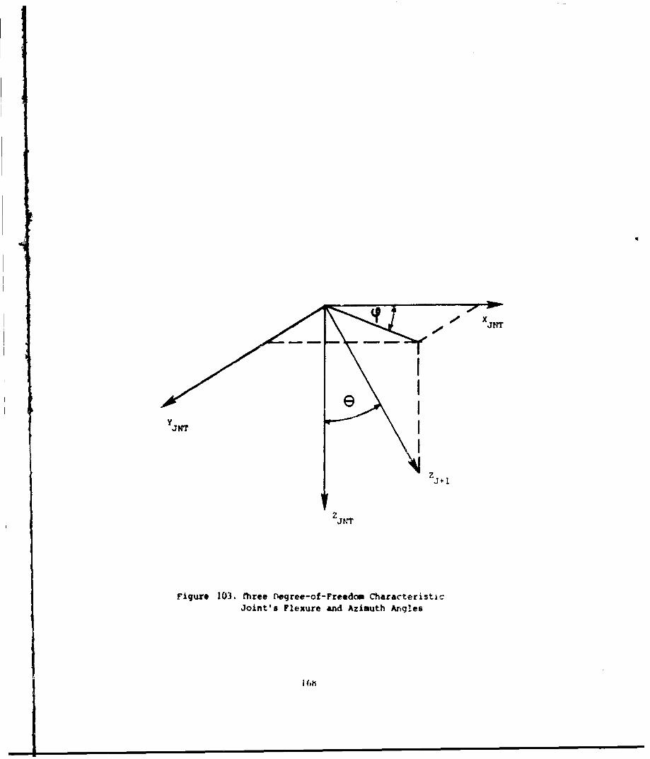
y JNTI
figure 103. rhree Degree-of-Freedom CharacteristicJoint's Flexure and Azimuth Angles
I 6M
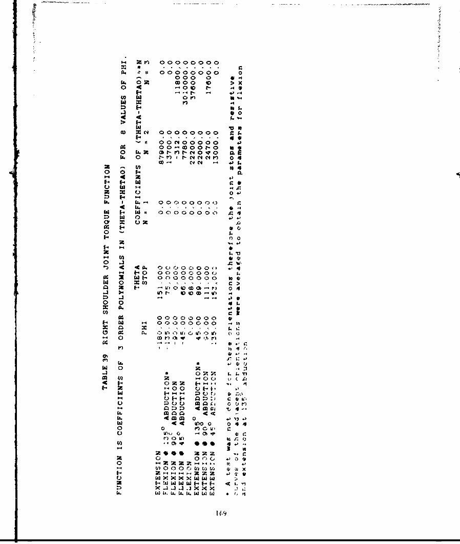
zro 00000000
" 00000000 0000 0 0 X
Ii. 02 zO CD000 44 -OO r C -4 0
1-4 L'-ul U) 0~ r)6w x r)
4 0
w X" 00000000 CA
SNOOC'00000
0~ ~~ 0a. G-)-c.~ 00.20 IJ6 A " Ot- l-NOVOW 0 r-n I rl-Nm"" 0 4
NC4 4 + 4to o
0 0 14
1 0 000000(.3 '
4 14 . 1 6 .
E- ifO 0000000c)
4 Ia 00000 6"U) o4 U).. . . .. ..- . >
Sw o
o o 20'-
f4 00
2-4 ~ ' o o .. .-
0 -..3't
I') 4 4. C) 0 ,00- 4 "0 00000000
S2wt- 00000000 ~14 0 ci . . . . . cQ 2 - U) 'i0 0 l- P) 0 4
0 0O 0.
I- w000000000
M- in C0 if 0 : 1c 0/U~ 0
C4 #1 r- o o o o -z
'-4 .a J-,.. 0",J ,0 X9
gV)0 C) IF-
macs 0 u49 Ol t, ofCt
Lac ccjc c(a. 4W 0 f
U) 44 tic too 0 4410 0 I)~
Zi :a0 *@ z .. C.
2 0 0C .0o0 '- 2: Z Z " 0 4 . W, 4
'-0v0000Wtac 4;IZ1- 04P4 Z Z Z 0 .11 0'I
Ua. W ti. LL. tL. It. WLCL) LI a t, el
1 f9
0 0000 0 0000 0 00000 . . .. 0 .C . 0 . . . .0 0000 0 0000 0 0000
GDO 0 0 000 0 00000 0 , 0 0 100a0 0 t-.. V .
M OOOO 4D V ) 0 4OOOO O OOtO-4 .. 4 -4 -Q
0 0000 0 0000 0 00000 1 . . 0 4 .0 . .. .0 0000 0 000 0 0000CO Mq -o O DO or OOor O M OOO
v, N CIO -,. C4 (1 ) M 40l '4 I ln IV 0 In 0
0 0000 0 0000 00000 000
0 . ... 0 o1 1 .0. . .0 0000 0 0000 0 0000 0 0000
OD000O400O 0 0 O 0 ** 0-'0 0000 0 0000- 0 0000M o q 0 0 O00D
'4 14 -4 CO U--1 -. 0 V ) Gb CO IOD CD 0 Cq' 4
: 0
, ,3 0 0000 o 0000 0 0000 0 00000 0 r o * * 0 I 0
10
P 4 0 0000 0 0000 0 0000 0 000oow > OD 0 0 0 0 00 0 0 000 co 0 0 0
0 0 0~r' N. b- 1 0o 1 N C, O ~C4 in" 0 M or -4 4s
11 x
0> o
1 AC 40 0000 C 0 0000 0 0000Ca 0 I-,0 O 1 0 099 It. wO 0 0 00 *) (>~0 0 0 u00 0 0000i) *c. 009)0 CD 00 0 o000 0 CD00 0
44 - W (In) M' - t-OD ) 0 0 0CD n i
' UC)~ 000014 -4 -- 0000
0 1' 0000
IL. 0000 0000 0000 000040000 0000 0000 0000
114 0000 0000 0000 0000c OO O O 0O O % b w 3 o 01 Cb
. . . 0
4rt;A 4 *, :?4 " 4:24M- 4?.C
X. Is) o Woo 44o oooo wIj x[aw1 X
.9' 'h. I f I . 4I ,' I 1 t. I .I . ( ..
170
o 0000 0 0000 0p 00000 . . . . 0 . . . . o I0 0000 0 0000 0 -0000 0000 * 0000 0 0000
0 In0.0 0 C000 0 C400VIn tfV)') 0 t- 0 )O 0 in (Din r- W
-4~-~4 14 .4
0 0000 0 0000 0 00000 ..... 0 . 00 0000 o 0000 0 0000
00000 0000 0000
0 004C 04 o ) i 0 0N 0An o
X -
0 0000 0 0000 0 0000 0 0000
0 0000 o 0000 0 0000 0 oOo
2 g 0000 0000 0000 00000 m 0 -D0~0 CO 0 40 (D a 0 O IVC1 0 40MOD0V4I' I) - C in 0 v In c*4 v r) CIO VC )40 N
0 OD V.Cm 0
U. mw
w 0 0000 0 (.000 C' 0000 0 0000D 0 0 *1. . I C Icy 4 0 0000 0 0000 0 0000 0 0 CC090000 0000 * 00000 C(.(.C0
0 0 [-t0.QC' 0 .'.I . 0
-71 -0 0 100 00 0
s-4 -4 C,
E-40 000 0 00 000o: o 0 0
0 F -c
0- 00000000 0000000W 4 0000 *0000 000 0000(0 0 C.-. a 0 In el 0 CD0 06 0r
0
44 Z4 04 0004ZC40X. Z
WF- I-( EC - -F.wI F --I4 c- c 4 X - c x 40- ILI 0000 )
E171
o 0000 o o00 o 00000 .... - 00 0000 0 0000 0 0000
0000 * 0COC0 000040 0000 o N"O") 0 0000
0 0 qv 0 M'~.0' F) 0 P) q qco C4~~~g -'--'0 Cq 0
0 oooo 0 oooo o 00000 .*.*. 0 . . .. 00 OC00 0 0000 0 000
0 o0 00 0o00 0000 CO D D. 0 D CD O 0 C.c
we IV M o o 0 o o - o o o D o
OCC0003
5 0 0000 0 0000 0 0 00 0 00 001.. 4 0 . * 0 .'. 0 0z F4 0 0000 0 0000 0 0000 0 0000: w 0o000 0000 00W0 0000W 0 00 O Io0 0 ;000 0 0 460 0 C4
V) 1 0 r) )( ) 0 t- Ob00) 0ID-0 0 o -to1-S4 c 00o
or 0 --
0 V)
0 0000 0 0000 0 0000 0 0000w 0 0 0 0z 4 0 0000 0 0000 0 0000 0 0000
>. 0 OON OCIO 0 0C40 1 0 0OD0 0 0 %V006 .ro l 60 0 1064IV -IF 0 0#0 00A 0 CO C t C
t 4v C4 r) r4 tv C [, (ID fO0 C'# r- C14 r- t- N N ODC*4N4 N~~'~ CI -' #C4 b
o3 0-Co 0000 00000 0 0000' 0 00000 0a WO 00400 o0000 o0000 00000
M- 540 C4CID~ 0 1 040r40 00060 0 0OD 00 '4 N~ - N 0 0--41 0IV60 0 I ID qv
2to f- CDC -W CD 40 to V) -
54 .4 k
410000In 540 0000
W1 w- 1-4 0000
O x 54 000041 0
5-4
0000 0000 0000 0000hi 40000 0000 0000 0000
10000 0000 0000 0000
0 00 0 0 0".j X -' 3 - -3 BA "4 I3Z
0 0 U 4ct I(A404 iz 90 a 4 29I 0'v4 W. Z 4
) 4 4c .4 4X x o4x 4 .qcx4
172
o 0o0 0 0000 o 0000
0 0 0 0 0
* 0000 - 0000 00000 0000 0 40 CD0 O 0 0000
0 0000 0 0000 0 00000 . . . . 0 . . . 0 . . . .
0 0000 0 0000 0 000c0• 0000 0000 00000 qrC40 C 0 qrcq0 N 0 40 C0 C
(4 4C rt 0C4O "C
0 0000 0 0000 0 0000 0 00000 o - I 0 . . . I. . 0 . . . .
0 0000 0 0000 0 0000 0 0000
4 0000 0000 0000 1 00000 #000 00 00 0 D 0 CD
0 00 00 0 0 0000 0 0 0 00000 I 0000 0000 ,.0000 0000
-a 4 ON0 C M 0 C4 W) t 00 0 -0
w N 0o0 0 0
0
0 ooo 0o 00 oo.)0 0o oooo C
w 44 0 0000 C,0 0 0 000 00
W > 0000 0000 000 0000
0 0 0 0
44 r Cbin0M0 - Nf-- c 0000 t- t- 0 00
I,. 0000 0000o 0000 00000
0 31 0000C0 0000 00000C 0000
U.=- 00 0 C) 0 00 00000 0
qc4X 4cC V1 v0 - 0C DO
w .73
In
modeled as two three degre*-of-freedom characteristic joints on either
wid of a rigid element. By doubling the stiffnesses obtained frcs the
static test, similar results can be obtained for the joint torque with
the model.
A similar method was used for the hip joints. The test curves were
digitized at ten degree increments of flexures 9. and these values used
in the table. The slope between the last two measured points was
doubled for each subsequent ten degree increment providing a stop. The
left and right side were averaged to obtain the data in Tables 44 ard
45. The equilibrium position defined for the seated dummy's hip is the
orientation with the upper leg extending straight out in front of the
lower torso and for the standing dummy's hip with the upper leg
extendir*l own fro the lowe.- torso. These orientations are defined by
the hp joint axes.
2.2.1.4 Skin Compliance (Mrictoristics
The AT, modoit s force 4e.lectioa chracteriatics are very flexible.
allowing the function to be constant, Wadular. polynceial or any
combination ro two of tiae forms. for the rangs in *hich the
deflection was tested, it v decided to uie the polynomial input, since
a wwthod was svailable in which severol test curves for rach segment
test could be averaged to obtain a stigle polyvtiniol Beyond the tested
deflection, tabular data were asdea to provide the model with a bard
stop. For each surface tSted, the tebulor 40t& points of force vs.
deflection were initially plotted. There vwrt, often 4 to 5 of these
plots for each surface. Thy *ere compared for jeneral &hp9 and ranges
of fore* and deflection. It there was one set that did not fit the
trend, it was not uoed t, find the averuged eut-e. The data points on
the loading portion of the ;.uive ver? fitted to s univeriate curvilinear
regression model using orbhegonol palynosialt. The curves perteining to
the same surfact were averst4d to vbAin 4 'Any,;e. polynow.al for the
curface wit!, a charocterixtic a. shown ti Ftiurt 104.
I 4
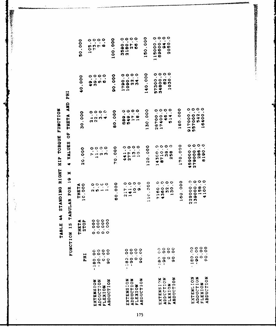
0 0000 o 0000 0 0000
0 tV) 00 0 t- 0 0
0 0t 0 0 0Co C4 0040
0 -4 0o' 00 000 In)C In 00 C4
0 0000 0 0,000 0 00000 ***. 0 ... 00 0O000 0 0 0 4 10 0 00 C4 0
40 r6) ~ C4 V) 0 0 0 r00 1- 0 0 O)w 0
00000c, 0 0000 0 0000 0 00000 0 .* .0 0 0
2 (k 0 0 co 0 0- 0o 0 00040 344 to) V 0) 0 0 Wr 0
C14 V4 CO fos 0 .4
13)0
0 >C 0 000 0 )0000 0 0 0 0 0 0 0 0 00
t-4 .J 0 0 0C4 0 4 r--) 0 -tPC 0 C,0000O 0 0000
4 0 -4
cor-' . .4 )me el 0 in V.t o 0 0C
C4 460 CO Ob 0
C)C~
.40 000.0 0 0000 0 0000 0 C. 00 0
f40 0 0 . . . 0N 0in0 M~ 0 t- - 0 0 0 o0 0 40 0 0 0D0
.44 q. 04 0 r) r) 00600
C) 300 Cl4 .V) p4 0 0 v4
2 C1 to)4c4 ClV4
40 0000w (A 340 0000
13 0000
4 234 0000-44
00000 0000coo
OD. M4 0 0 OD000)
00000 0000 17.0 0 000
t-b 0 E4 n t 01 t. w O 01 .) f-0z - I :
00 0 00 0 CO 0 3
34WC a ja) im A
175
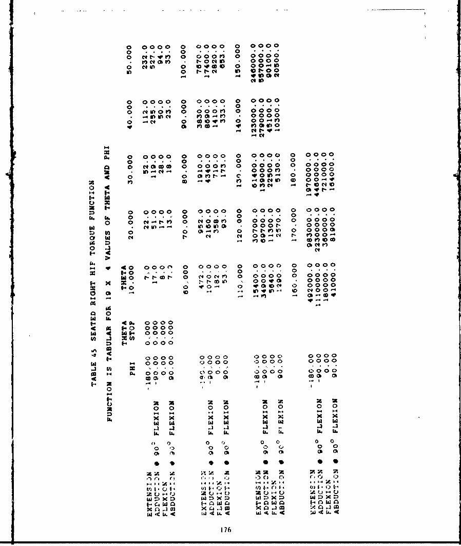
II0 0000 0 0000 0 00000 . . . . 0 . . . . 0 . . . .
0 eq - 40 V 0 000"' 0 0 00 0V Cq 0 r) t-0c in 0000
40 Cq in 0 come 0 00-0VC) ~~ ~ i 0 I' P 0 0
0 0000 0 0000 0 0000
0 00 c000;0 0 in in C4 0) 001 -) 0 0000
to V00 t) 0
0 0000 0 0000 0 000o 0 00000 ... 0 .... 0 .... 0
00 e41( 0 000r) 0 0000 0 0000
N PC4 * 00 0 M 00004 0 00 0 )I-o c IV o00o 0 0000
0 f OD r) -4 0 I0
0 o q 04 OVC et-4 V
i0 0000 0 0000 0 0000 0 0000S 0 .0 0 0 0
0 0 1' 0 COCD) 0 0000 0 0000
I 0 0 0 0 f-)C) 0 0000cN 0 q c @ e - V000
::) 4' 40A0 0 00 0 00 0 0 00
2 ~ ~~ M4 40 CID * 0 *
40 -000 0 0000~t 0 0000 0 0000
W 0 f- 0 Of0CsI 000' 0 0000
2 40 0 q0- 0 q(0 0 00000 b .- 40 ." P 'V C40 0
644
0 0
*4 400 00004 0 1-0 0000W 4 w*1F4 0000
~2*4 0000
*4 0000 0000 0000 000014 0000 Q000 0000 0000
0 1404 0000 0000 0000 0040
0
0 00 0 0 0 0 0 0
. 3 -1 .-1 .3 - .4 -3
0 00 r.0 0 0 000 0 0 0 0 0
* 4 z;, *
.- C; 0 *) ) ri 0 Q
*4 0V.#*" 4 ; 1 .
E- 4 w Xf. Wi 10 w a w
1 176
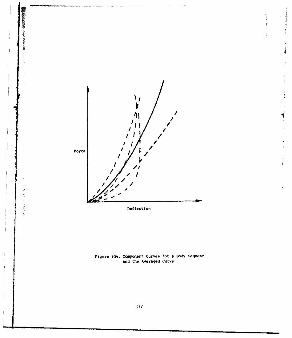
Force
lopI
Def lctio
Fi'1r /04 Copnn4uvsfraBd emn
/ /17
Tabular data were used to model the second part of the functions beyond
the test deflections. The force at the last deflection input is used by
the model for all larger defle.tions. The tabular forces beyond the
tested deflections were chosen so as to avoid problems due to this by
providing a more definite hard stop.
Table 46 contains the input parameters for the thirteen displacement
functions. These parameters are defined in figure 105 which is an
example ATB force-deflection curve.
It should be noted that these curves are based ont the date from the
tests done with 1.0 and 2.5 in diameter saucer asnaped probes impacting
the surface. If the user wishes to use these functions to describe the
co.tact of one of the dumy surfaces with a surface significantly
different from the saucer shaped probes that surface's force-deflection
characteristics should be combined with this data to provide a mutual
force-deflection function.
17
178
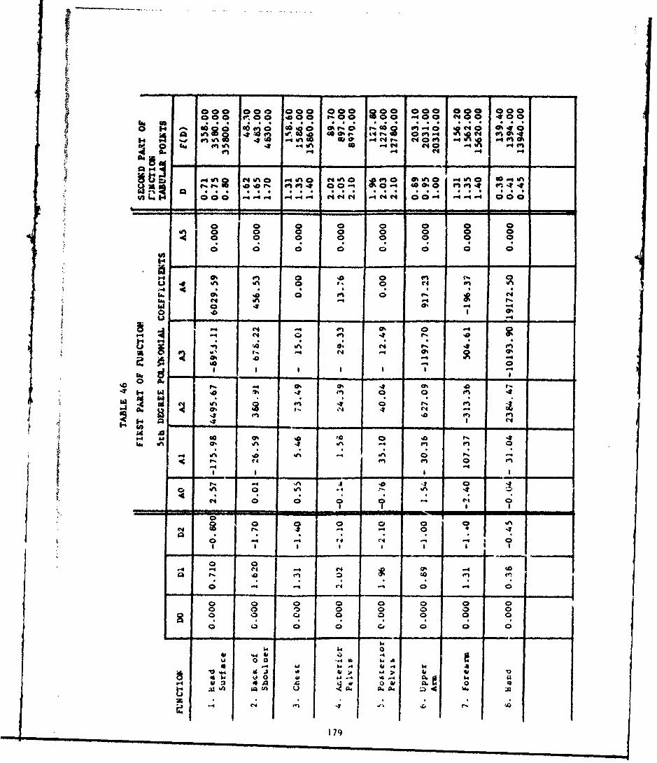
000 00o 000 0 00 000 000 000 00Q00 a e a0 to00 v.0 00 a a 0 ('0 a 00
hi . . 4 * 4 . 6 *
%.V EzU' 4. 00 4C0c4
0~0 %A inmI C4W 0 en(4 .0 - ~ -4
NO4'~ .- VI r% ~ m 00 0 44O
0 4 4 44 . 4 4 44 .4 t4 C . .-. 4 C; 4; 4
0 0 0 0 0 0 00 0 0 0 0 0 0
m C1
P-. 4 4 at .
0 . f' -.4 0 Ch(6.4 W4 44 -f I.
LI t-
C1.4 C44
04I -4
'0r W.4
0 a-4 0
g 14 W o.4 4v 0
W) 6 a l - C6 -A-
L179
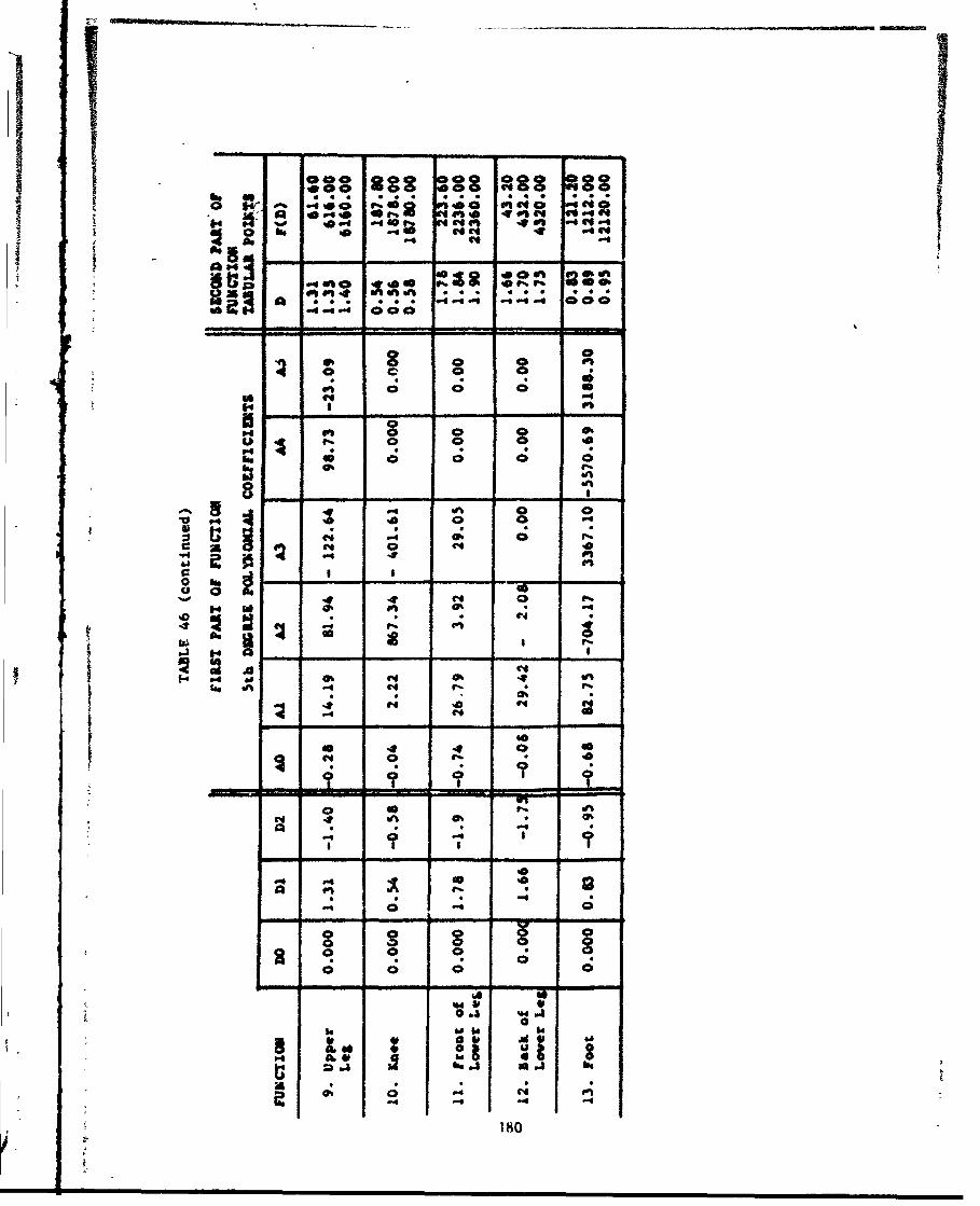
00 0C40 A~
4104 *0tU ell 4'5" 0 4f'ct C4
... . * .44.4 t.4.. 000
WI 0
0 0 0
1* @4lei
I18
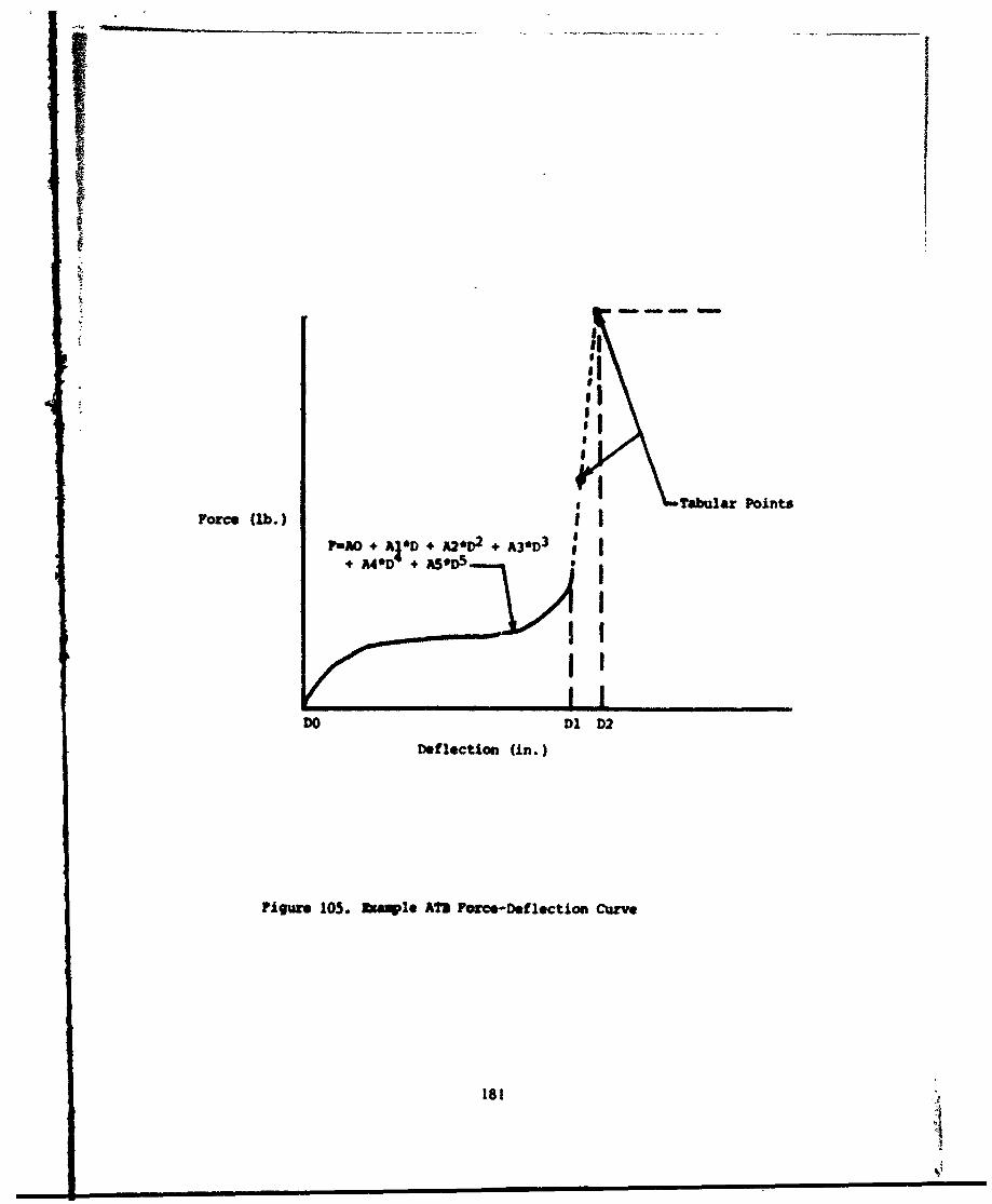
II
Tabular Points
Force (lb.) I..Ao,+ Aj*D A2P 2 + A3*D 3 g I
+ A4'D + AS 5 S I
fVI'DO DI D2
Deflection (in.)
Pigure 105. Exmlple ATR Force-Deflection Curve
181
2.2.2 eoratiom stisms
Desogtgm simul4tioa nsit the WSIAS moel we perfogmed to
use tba the inmput data bad been prope 7 femattd, the nodel
proSrem w d tim vith tee data ad the data reslted is lqaskAllyrealistic slealatee. Suck demstratios would at least guarantee to
subsequen users of the data base that the simimlatio should execute end
that phrsiclly reasomable reults should occur. These simulations were
net mode for the ratqoes of the ybrid II data ba validatiom.
A siaulation ws ebsem that had previously been perfomed witk the
standard Part 52 data base. This simulation was based an a Celebrity
frontal impact crash test in which a purely -z axis acceleration ws
applied .ith a 239 peak amplitude. 120 millisecond duration, and a pulse
shape that resulted in a 31.3 mph velocity change. No harness restraint
was appliod to the body. The interactive surfaces used in the
simulation were for the seat back, seat pan, floorboard. footboard.
steering wbeel. windslield. dash sad roof.
Three simulations were perftomud using the Part 572, Hybrid III seated
and Hybrid II staeding data sets. The vehicle geometry and motion time
history wet identical for all three simulations. The initial positions
for the Hybrid III data sets were adjusted to be as close as possible to
the Part 572 poeition while maintaining initial body equilibriun with
the external interactive forces.
Dbth time Listories of the responses and graphical kinematics wereobtainod in the simulations nd compared. from an examination of the
time histories no numerical instabilities or calculation problems could
be identified and all predicted response values were within physically
rasomable renges. A comparison with the Part 572 time histories showed
that Hybrid III responses were in general quite similar with primary
differences being phase shifts. slightly moother response curves for
the Hybrid III and also somewhat faster responses for the Hybrid 11.
182
lo efetaee nepee to be respectively due to si gtly
Graphical apismofO be i stosaesasi iua10
j572 dum saomt t~*105. Mwe resp...., through the first g
m~iscooe at *Msiaar.A aeaiingly much softer ftmerion neck
q is thePast $7 at about 120 siecoeds wen tbf# headImpats he indbiod* haMybrid III seek do~es mot under&* nearly asne amck exesmedrebounds f rm the steering wheel, windshield
and doeb impact abso thenw the Part 572.
The responses for the seated and standing Nybrid III are compared infigure 107. There is very little difference to these two responses.The only readily observable differenc. is that the seated dummy
penetrates deeper into the neat pan than the standing dummny and thispenetration increases dtriag the course of the simulat ion. A comparison
of the Part 572 and Oybrid III standing dummy is shown in Figure 108.sn" the staWmia and seated dmy responses were so similar, the
ceipari-io cinents for the Part 572 and seated dumy apply bore as
wall. The only dffterence is that the seat penetration for the Part 372and standing dummyi Is about the "w "s opposed to the seated dummywhich exhibited sueh greater penetration.
183
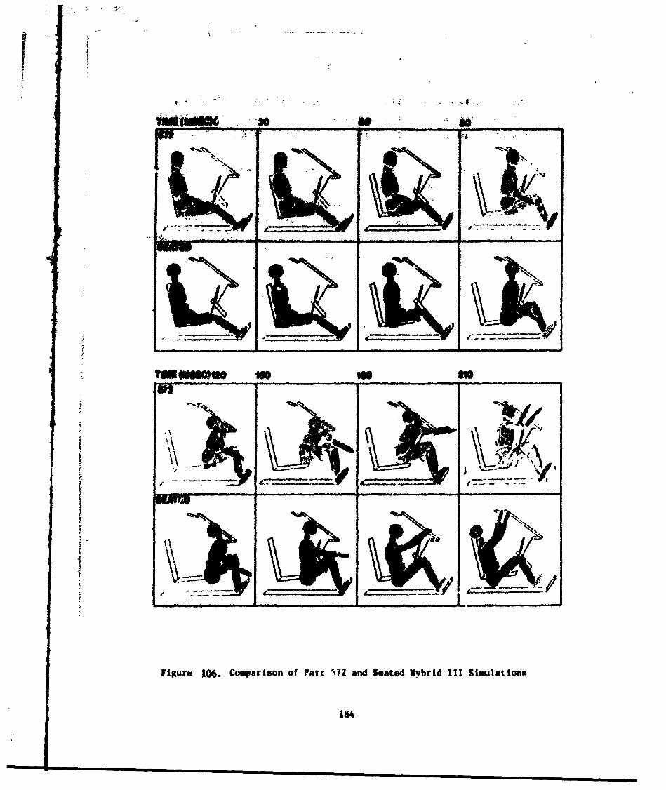
1wfw
I'1
FLKure 106. C0"4~rl*On Of PflrL 5172 and Seated Hlybrid III Sloultimos
184
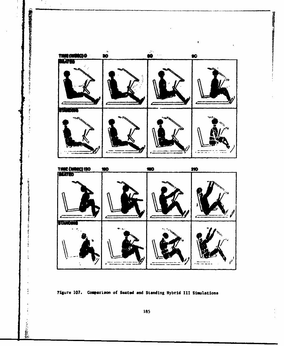
" WN
( -,~,0
tuI~@~Ag
Fi~re10. omarso ofSete ad tadig Hbrd IISiultin
185~4~
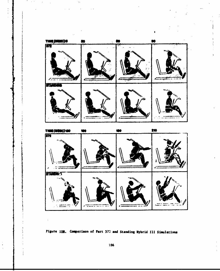
4I
I'~~~I - d .-.-f--
186~
2.2.3 Discussion of Results
The general objectives and approaches used to develop the Hybrid III
data base in this program were similar to those in the Fleck, et al [1)
study for the Part 572 simulation data base. One additional aspect that
was addressed in this study, and which influenced the data measurement
aud model data base formatting methodology, was the development of
transformations for relating the dummy data to human data. This was
achieved by defining equivalent human anatomical landmarks on the Hybrid
III dummy and deriving transformations between segment anatomical
coordinate systems, defined by these landmarks, and the mechanical
coordinate systems defined with respect to dummy structural features.
e.g. joint centers, joint pin axes. etc. As dummies attain greater
human-like fidelity, the coLparison of human and dummy responses during
dynamic force exposures becomes more meaningful and the availability of
such transformatiors would make such comparisons possible.
The dummies for this study were selected to provide a data base for
automotive and aerospace researchers. For this reason, one of the
dtmmies was a standard seated dummy, with a pelvis molded in a seated
position, designed for car crash testing, and the other was a pedestrian
or standing dummy which is more appropriate for use in aerospa.e systems
testing. Aside from the spine, pelvic section and upper legs. both
dummies should have been identical. This was not found to be the case
as was clearly evident from the measurements made on these dumaiec.
While the final data for the parts that were identical were averasfed for
the two dummies and for left and right sides, the variability in these
properties indicates that all Hybrid III dummiec are not alike. It
would be well if some future studies could be conducted to investigate
this variability over a larger dummy population with different
production dates and use frequencies.
The formatted simulation data was run on the CVS/ATB model and gave
physically reasonable results. In a comparison to ;quivalent Part 572
responses under the same conditions, the Hybrid III simulation had
slightly higher peak accelerations and quicker rebound, but smoother
time histories. These characteristics seen to imply that the Hybrid III
is overall slightly stiffer and that its data set leads to a more
numerically stable solution.
While this is the first comprehensive simulation data set for the Hybrid
III and should be quite useful for simulating Hybrid III impacts.
several issues should be resolved before such a data base can be
accepted as a standard. The first saoung these is whether the dumaies
tested were reasonably representative of the Hyorid IIIs in general use.
The question of property variability, especially for joint ranges of
notion and bending resistances of necks and spines, should be resolved.
Also the current study almost total ignored, except for the neck and
spine elements, rate dependent or damping effects. These obviously have
some effect on manikin response. should be further explored and should
be added to the Hybrid III data base.
Finally. the most important consideration in the Hybrid III data base
acceptance is whether it represents the real world. To demonstrate that
it does. carefully conducted validation simulations against well
controlled experiments should be performed.
188
REFERECES
Fleck. J.T.. Butler. F.E., and DeLeys. N.J.. "Validation of the
Crash Victim Simulator." Report Nos DOT-HS-806-279 through 282. 1982.
Vols 1-4 (NTIS No. PC E99. PB86-212420).
2. Personal Communications with Stanley Backaitis. National Highway
Traffic Safety Administration.
3. General Motors Corporation. Hybrid III Quality and Performance
QualificatioD Manual. Safety Research and Development Laboratory,
General Motors Proving Ground, Milford, Michigan.
4. McConville. J.. Churchill. T.. Kaleps. I., Clauser. C.. and
Cazzi. J.. "Anthropometric Relationships of Body and Body Segment
Moments of Inertia." AFAMRL. Wright-Patterson AFB. Ohio. TR-80-119.
1980.
5. Young, J.. Chandler, R., Snow, C., Robinette. K., Zehner. G.. and
Lotberg. M.. "Anthropoetric and Mass Distribution 'racteristics of
the Adult Female." FAA Civil Aeromedical Institute. Oklahoma City,
Oklahoma. FAA-AM-83-16. 1983.
6. Lephart, S.A., "Measuring the Inertial Properties of Cadaver
Segments." Technical note in Journal of Biomechanics. Vol 17. No 7.
1984.
7. Chandler. R.F.. Clausen. C.E.. McConvilie. J.T.. Reynolds. HA.. and
Young. J.W.. "Investigation of Inertial Pxoperties of Human Body
Segments". DOT HS No-801-430. National Technical Information Service
(USA). Springfield. Virginia. 1975.
8. Bartz. J.A. and Butler. F.E.. "A Three-Dimensional Computer
Simulation of a Motor Vehicle Crash Victim," Calspan Technical Report
No. VH-297-V-2. 1972.
189
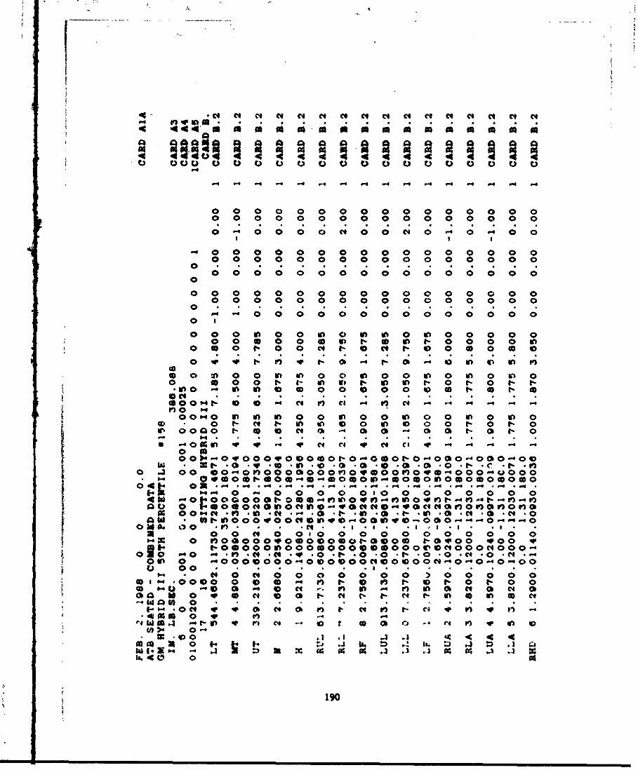
4-j tc4 Of C N Ni N 1 N
44 444 44000 000
t) C Du 00 0 0 u D0 a 0 0 a
0 0 00 0 00 00 00 00 00 0
0 0 0 0 0 0 000 00 00 00 000 0 0 0 0 0 0 0 0 0 04 0 04 0 0
C; C; IC;C
.0 00 0 0 0 00 0 0 0 0 0 0 0 0 00 0 00 00 000 0 00 0 00 0
00 0 0 000 0 0000 00 00
000 0 0 0 000 000 0 0 0000 0 00a00P.000t-0 0 00 0
0 a 0 It 0 0 t- * 0 t- 4 4
-0 "0 0 0 0 0 0 0 0 0 0 0 0 0 0 0
0 000 0 -k )1 0 1-O 00t-0 00 ti0 000 0 0 Pt- 0 Pt 00t-0 0 P
0000 0 0 0 N 0. ON 0 0 00 00
0D 0 U r- l 0 0 P 0 0P 0 0 0 0 P 0 tP 00 0 0 0* r- 0 5) C4 0 - 01 t- 0 r- 0
P0 '4 Pr 0 0 0 -q 0 0b 0o 0 .0 0 J- 0 t.. 0
asMI o" .a N n c a f 4 .4 .. 4 -4 C; C;-00'0 P P 0 P 0 0 0 P 0 P 0
at 000 -0 0 N~ -0 FAW *. ---44 4
Ogg-0 0.0fl000000000000000-'000-4000-
f)00oooI4-00 oo0 0 a M ro00 -o-000-.o0 f 0 0
0o 0 N 0 0 0 0 0 0 0 in 0 000 u 010 w 0 0 a ' 1. l f- 0 N 1-Wo 0 . 0 . d - V 4 I) P 0 N 0 C
0 0 C 0 - ( 'I- - -0 P t. C4t
F-.04 ON l v' m' N fo t C- l - 41 I') inmm0 F. b6) :D 3
'x .3 : 3 at .c 4 (4 A .3 A x10 1 4 .
190
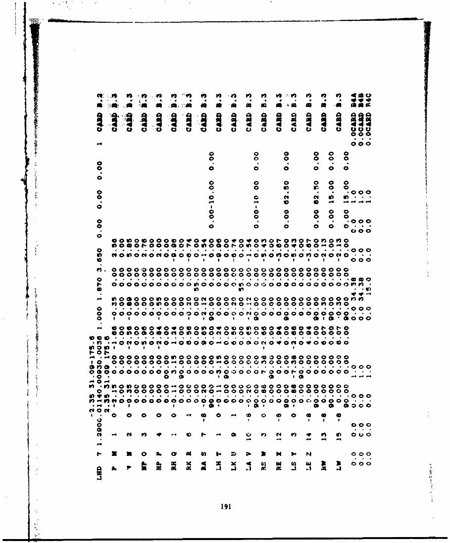
Ce ~ a -. Is 0 11 ) V) ig t a'n to a') ve V) n, to- to) A 4* 9 9 *, 0 40 0
* *4 44 04 4* 0a A 0BU00a
000
0 0 0 000 0 0
00 0 0 0 0 0o0 in rl 00
0 10 .0.00
0 0 0 04 C
o 0 0 00 00~~ - 00000 0 0 0 I.
000
000
00000000000000~00000000400-00
r 000000000000000000000o00000000000n
0000 0000000000000000000000000000r~o0 . ;C . .0000 0000O000000U00 0 0 00000000000000 ...
010,000
0 00000000000C400000t400000000000000 . s ; 4C . .. . .s'o
-r 0 000C0000 0U)04o 0 0 )0 4 mo 0I-0o
-- 00U0@0C000000C4oooU00000@000O0000010 '00U0C0-0000@0-0OO0O~cl040Cl4000
i- *-00000000U)00000U)000000 30000000090*0 00000000-000-0OOCJV)00fl0000000
0@00)C0000000F)00000V0coco0to00t0000000 ..
00000 000 0 0 0 aO a44
-4-4
xlC4 0 0 0 A$ 0 0 0H z > 000
A. x 4c v) od 4.w 1 oc4 9
191
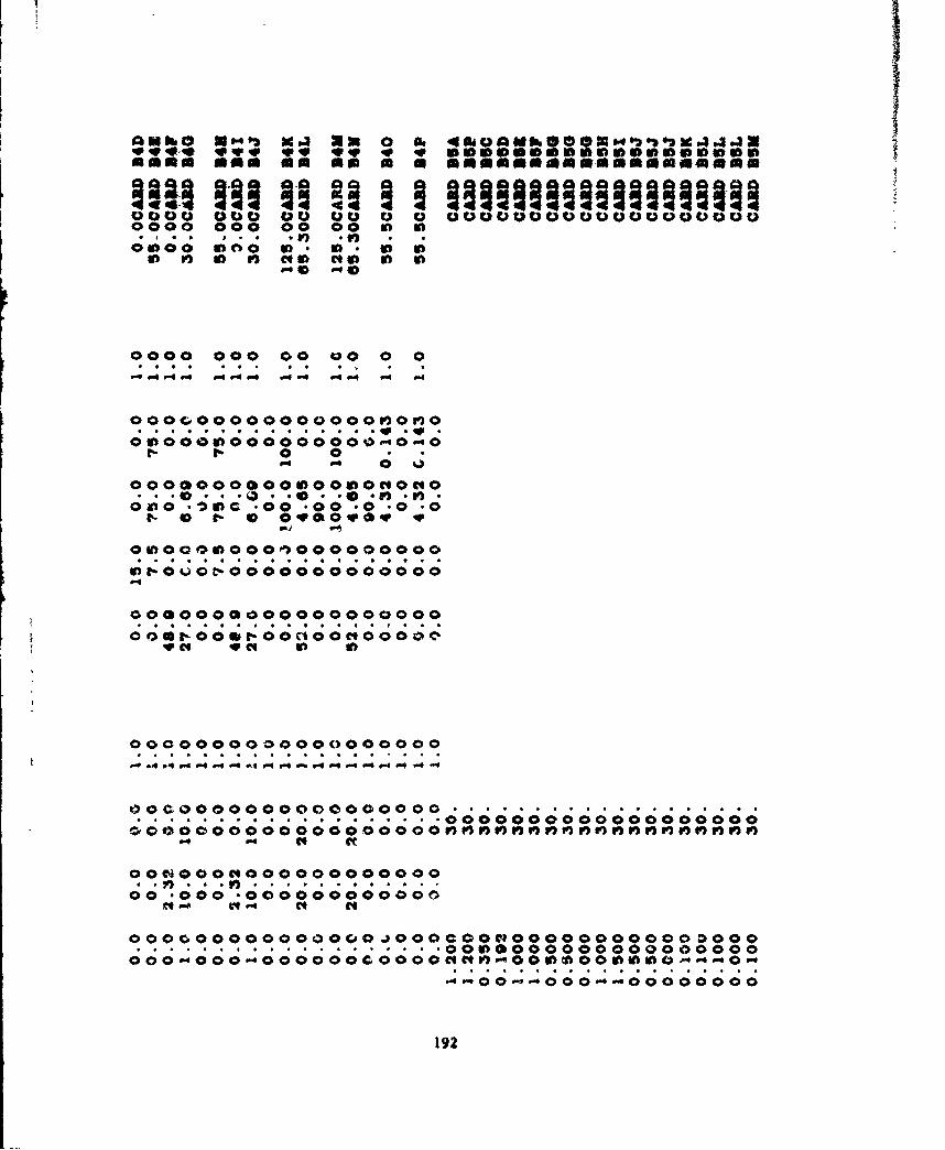
ovoi U..' ov 0 0a *s m o a moosmmeo 0.0 MANAMA wonb~~b~
000Dc aD a aeaaemaaao
OUOU 00 00C 00. U. 0 0 0 0 0 0 0 0 0
0000 000 00 00 0 0b
.4 ,-4 * . a; .4 * .W ; ) . .
00CW00 Sf0 Sb. Sb. Sb S-p .p
000 000 C ; C 00 0 0 0
I.-0 0
000000000000000r0r40o* * . 0 ( *000 *.* P V
000o *,:oC -00 -00 -0 .0 .0u- r * oqeoovov w
000000000000000000
b f- 4 0000000000000;C;q 4 4;C;C;C0-4
0003*0000000000000oc0
0 0C0 0 00 0 0 0 0000 00 00 0 . . . . . . . . .
.0000000000000000000
O0O0O"000000000000,I)'
00-~000c000000000000
" .4 C4- #"
o000O0000ioooco0000'IQOOOOOOOOO 0000... 00000000000000000000
ooo-ooo44 - ocooo C* 0000 ""nV-000Sb000 - --- 0---. 00--000--00000000
192
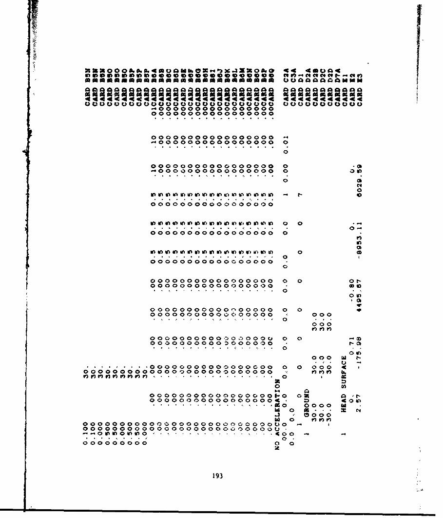
0masmmmmmm~mmmmanmmma~mm UOQOQaM
11F
0 000 o000000000
00000000000000000
00000000000000000.00000000000000000 0
0
00000000000000000 0
.0004.000000000000 0 01
0
0
, o o --0 * 0,0 *0 ; ,0 ,0
ooooinoo i nt nIti ni ntoft to o 00000000000000000
0 C00
o 0
00000000000000000 m* 0-
00000000000000000 0 0
00000000000000000 CDC0
ome) 00
*00 0 0000000000000000000 00 0000000000000000000 00
00o00
.00000000001:10...0000 0 0 0c
CC000. .. 00000000000000000 0 000
0
0000000O000000c) 0 00000000000000000. 00
1% o 000 0A 000 IJr
o OOOoOOOOOOOOOoo 0o0 000 4
00 0 0 0 0 0 9 000000000 )7' . La..... .- 0
0 U)c; 0, 0* 0000, 0' 0 0 0~
193
, l l I I 0 0 0I 0 0 I0l 0 0 l . l| • Mm
460 46 46 4 4 ON 40 46V- ow Q "vV0O oV "V - nV0- o
-e - 40C
o 43 a 0 0ll- 0 0
o 0- 0 00 0 00 0 0 W *P3 0 01 0 0 0t* C01 0 VW4 -0- 0 - O 000a03) " 00 4O; 0 * -. U' r(* * C; *- *. _; - * 0
0 tv -rO l 0 0 U-04 0 -0 4
OV V
on CA to " n .0 b > - ID -OV0 O. t a 00 of :P, C4 4-- 0 0 1 e C 00 4 i - r
C) co -4. 6d to r) ef 0
0 -~0W4 0 0 0Id 0 0 00 0 0- -
W- 0~- oa4n - o o 0 0 4) n *
0 "? 4 z 4C 34
C10 0 *mo 0b-4- 000-t- *A0 o * 0 0 r 0a
0.- M -o 0 0Jw a 00 0 U. o-40
S19
* 0e -
0D 0 0 P4
.n 0 Op .0 a
ie a0 if 00 0000- - r) - 00 00 0
m0lr
OW a a 0 0 * V l 0 In -0 a0 00 00 o "~ 0 00 00 0 - 0
0 r- 0 - 0 0 0 0 to
* I-n
-if W" MAMO 0 be - -e -1 -0 -00000000.>
oe .00 t- -. 3 0 t - I .--t -9 - - r) m) - -00000000
irfo o 0 Ca 64 U- Ct 000 0 f iIf 0l .l C4 if id 00
CO - Id 0 O4t *r 4W s 0 a aD1M- 0 000000001On "wo -P 0 0 - 90 0 0 . . I .. . . .0c.0 00
I- a4 0 SK . 4 .0 0n 00,0 0 a- 0IS -X a' 0- 4 0 - 0 a 0It- 000-in.0
r) 1o IC 0)3 OtCV r-#(4 -
195-
4444 1aaa 31oaaaaa
00 100 000 co0o 000 000O
loC me*00 C 0 to fO necan r$ 0V 0 - on-. 4 nn 0 0* 0 V)n i0l
000 000 000 000 000 a00000 m 00 ; 00; r f0 00 f01*0 000 On0 000 -C-0 000O-000 CAo W * o 00 -00c sot-1 10 0 t -0 -
00000000 000 000 000 000 000 00000000000 m00 @00 woo Ono M00 Onoa 000 Ono -00 M-0 -no Ono -no40 00e 00 - 0 * V n d o o 0 nr- 00- no *Dat- o0 0 n 0 0flO C' Vg 0 caVf
0c000000 000 000 000 000 000 0000 C00 0 0- ef-.c0 0 - -0 -"n0 C 0 0 n )00 0 -O00 -. 0 0 o n O o -- o -en1-0 -oo Vcon 9 n-n -en C ~ n0 -0 ne 0*0- ng n g- 4e
0C00000040 000 000 000 000 000 00000000000= IO 1-00 000 r-no -. 1-cwo r-00NbC -ec 0o an x wo enr0 00 0 na
n 0 e1-1
hii000000001 V00000000000000000g4 V0000000-n-e~ooou OOOOOOOocgOon)OOM 00000onoWO-e0e t-G 1 0 0 11oo woo 0 t- 0 t- 0c 0 1-V. -r-o0 1- 0 0n too w f-o0 9
C 0 * 0- -q -l W e
196
a aa aaaao
00000000000000000000000000000000C000
000 0-00 000 000 000 000 000 000040 "00 000 000 000 000 000 000
*o 000 00w ooo ooo ooo ooo ooo*o .o not- o.n 00,- wo- now
* n") MOO 0019 -4t3 "0(9 0 v19 n )-1
000o+e 000 000 000 000000 000 000 000 000 000 000 000mo0 wo0 000 000 000 000 000 000
00 40 woo "0 OW0 000 m6w @04 VO"
*0 -- '0 09- -) 01- (9 0
-e 0 -09 e - n - w 1*t 0 C10W
to 0 - no I 4 4
000 000 000 000 000 000 000
. . . .. .. . . . . .. . .
moo 000 000 000 000 000 000 ooo-0 -00 000 000 000 000 000 000
4 - 00 @40 4(90 000 400 - 0(9 I 00-0 at- n-- 0-6 tl- 0-.6 C* 0 - i I
o 0 w (9 C 90- t(90 co 0 - -
000 000 000 000 000 000 000 c'.%O
. .. . . . . . . . . . .
1-00 0 000 00o 000 000 000 0000-00 40W 00V 000 000 000 000 000
n "m 0e0 o00 04 000 04 0V <0 W0 0 00 " " 01 "W"0 -0" -04 -n C# ) - 6 9 I - D --
Id
000 000 16 000 000 000 *i1O0 000 0 10
000 t-00 000 000 000 000 000 0)0W0 -00 a 000 000 Z'o0 000 000 0130
me .4(9 4 (0 v0 " -0 0 fl* 4010 CI - 14I-~ -W(V'4 I & 0 - t- 001 n4 b VC
C* 0W>
.A4000000000W V0000000c00000000oW W0000000
0 co0 1-00" 000 00cD 000 00031 000 000 -00 09-0 060 moo~ 000 040 040 V 0I(t4V .00 -(90 t-0( 0 0 coo wo 0400 V410 M 1-0 (9 00 (9 004r vo- -0( Vin- Q9 a)
w- f4 -1 - 0 - t>V40 V 8- M t-0
197
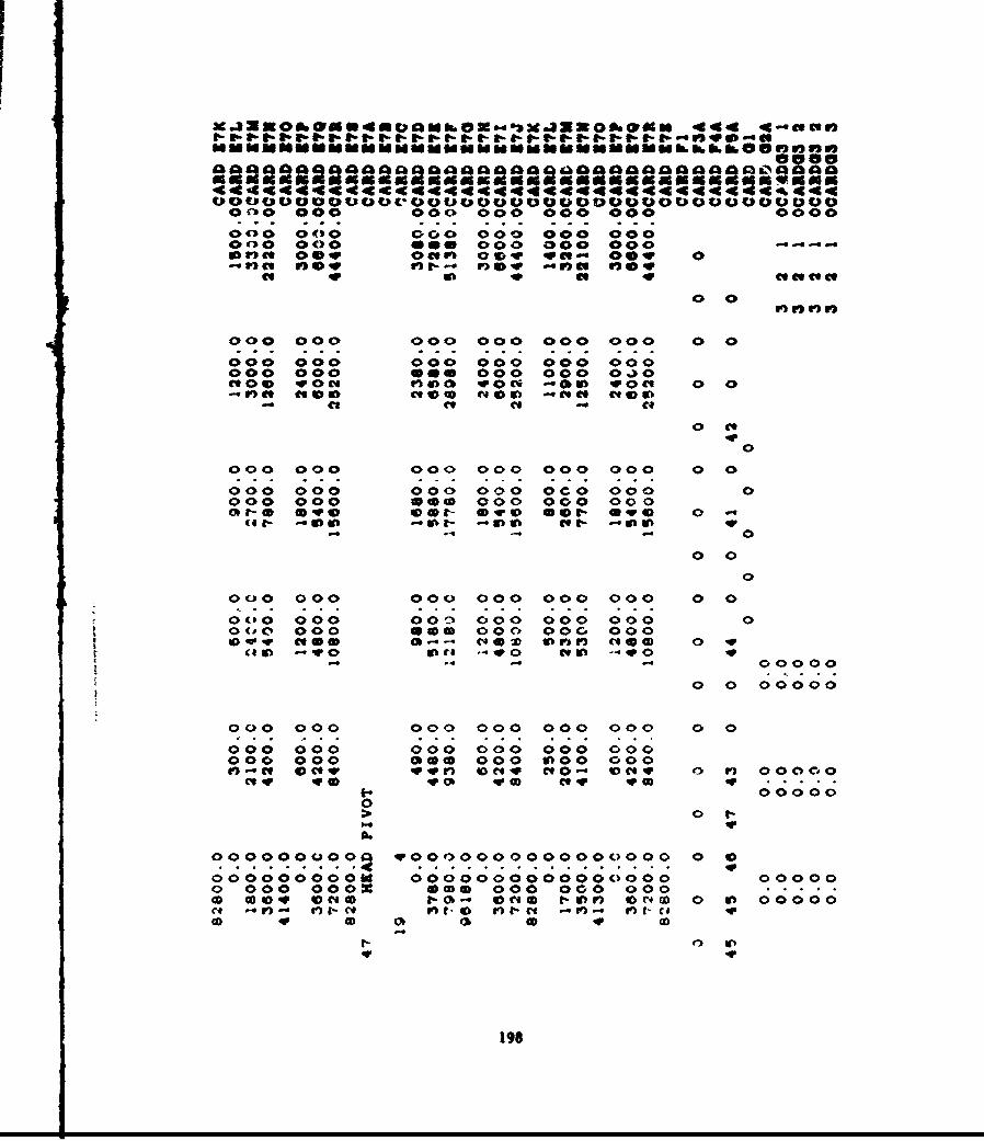
00 000 000 000 000 000 0000
0~~~ 0, . C
0*0 000 000 000 000 0000C00 000 *0* 000 000 00an" * Oen co W - 0040 0
n Ct ne 0 qv now -Oft " 0e IVVtC
0 0
000 000 000 000 000 000 0 0
000 000 000 000 000 0000co 000 00 000 000 0)0
tol (1 o c 00 wm 00 V00 '41( ft-ce re es - ft
0 0v0
000 000 000 000 000 000 0 0
000 000 000 000 OCO 00 00
0o0 00o *am coo 0oo 0oo000 000 000 000 000 000
- 00 00 000 0_0 0
00
o00 000 00" 000 000 000 0
00o00000o00000000o00 0000
o(' 000 000 m 000 000 000...
0 0 00000
000 000 000 000 000 000 0 0000 000 C;0*0 000 000 000000 000 *w0 000 m00 000n-ce ecw wwn OceW "0- ecMe 0 n 0oo000
0lw 0 0 W CD 4' V w0*. 00000
00 f-
000O0O0004 W0000000000000000 0 40S49 . .
000000C;0*C , 000.0(<>0000 0~ (>OOOOOOO OO <C)00 000000 000 000 acne 000 000 000W W0 V 14 V f% -0- 0(40 r-UlV ONM 0 in 0 0 0 0
CD0 01 1% V CD
-4p
IV V
198
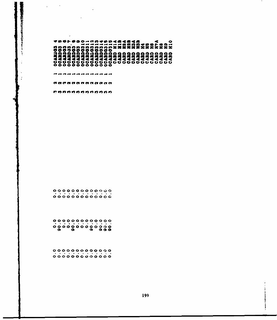
IWoo~l-e- ).r4 m4 4 o
@08g.th 0 Ooooo
O00000oO00O0
0000000000000
0000000000000
.. ..........
00 0000000000
0000000000000
0000000000000
199
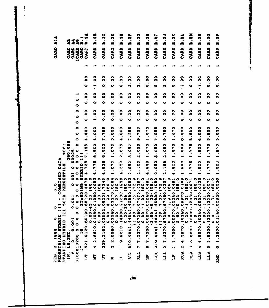
U 0 a 16 0 N = X~ X 0 ft0
.4 fl4 0 0 " * 0 0 -
0 0444060m0 * 06 0 0 U 0 0 0
00 00000 0 00 0 00 0 00 0. 4 . - . . . 4 . . . . . . . .
o 00 00 00 00 00 0 00 0 0
o 0 0 0 00 0 0 0 000 00 0o0 0 0 ( ( 0 94 a t 0 0 0 0 0
o - 0 00000000t-0 0 0 0 0 0
-0 00 0 0 0 0 0 0 0 0 0 0 0 0 0 0 0c 0 a - c- v r a 0 t- 0 IN - or
C ~ 00 an of 0 0D 0 0 0 0 0 0 0 0- 0 0 0o
a0 0 f 0 0 00 0n 04 00 0 0 0004
00 0 0 0 0 0 0 0 0 0 0 0 0 0 0 04C d 0 - N 0l 0 w 0p 0 0 0 0 0 0 0 0- 0
QA o0 0 0t- 0 0 a 0 0 0~ 0l 0- 0 0 00 0 0v 0r 0r 0r C4 0 0 t 0, 0q0 0
0 11,- 0 0 0q .0 .0 .0 0C 0 0 .0 .0 0 01 -0 01 0V
0 0 0s 0 - 0 0 E 0 ta.0 0 0 0 0 0 0 0 0 0 0 0 0 0- 0 1 0
*oo.-D o M -C4 (A ,-t - -0 -r 'n -v - Cql a.04" 00
1 0000 0 0 0 0 0 0 0 0 0 0 0 00. 00.4- 0-0 0V CJ O) ' 0*0 -4 aro WO w' 1
3W OO0000004000000000000O.0000000400
ag000000)00 0000 no00flF)0 4-0-0 00-000 p0q1 00 r . .o.- .. ooo . o.o. . o. o. o
1" 04 0 0 C40 Ci 0 0 0 00 0 0 0 0 0 0
ab > 0 f 0l0 04 04-C0 U-001 ca - 0 0.-0. 0 0 .4. .w .* .* .e .g . .
0.4 -oq 4 Cl -4 U -. . 5- 0 0. Na l
-am0 0 N0 0 0 0-,'004e)0.0404.0
ca o.-*0 4 0 0 4 0 0 0
*W -10054 0 ' 0 A F) 0 0 Cl 0 Cm0b3W 0 1- 01 Dl 03 0e 0QC - 0 C ) 0 0-(. .4 0 n z .ad g.a .1 . . a: . J w
116 (4. 0J Cl 0' 0 - 4 0 8- C 6)
0'0
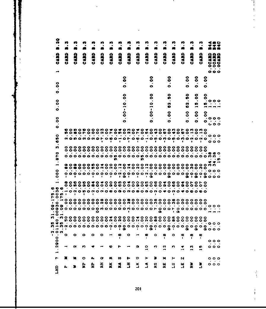
I
00 0 000
00a D000 0 V 0 0 g 0 0 0000
0 0 0 0 0 00 0 0 0 0 0
0S
o 0 0 0 0 0o 0 go t 0 0
0 .; a; - 0000 0 0 0 00-
00 00 00 C 0t-00C -0 0 00 00- 0 -0
0 .*.0000 S S S0 0 0 0 0 0 . . .0
00000000000000000 0000000 000 *0t- .00.0. . . . . .0.0.0. . .O.0. .000
in 0000000C4C 40t*Oq-C4t040-OoO OOOOg')01'30 -0 *000
00000000000000000000000000000000.54)00000000000 000e000000C000000
00 5a to in .II-*ooooooooovooomooooooooooooooooooif'0 OOOOOOOOCI00000C10000000V0000000
0 0 .* ...... *....000
oooooooooeooooos'ooooo-oovo-ovoooooo
000OOOO000000000000C00000000000000w o . . . . . . . . . . .. . . . . . . . .
0l~I'C000000000000000000000000000 0000fS 00 0 0 0 0 0 0 0 0 0' 0 0 0000
* 0 0 0 ob 0 00 IqI S S
O, 0 , 0 00 0.
0
t- X z3 0 4 0 )1 ) > 3 x4 >0 000
N. Ow X X 49 W t4a 9ds 000
201
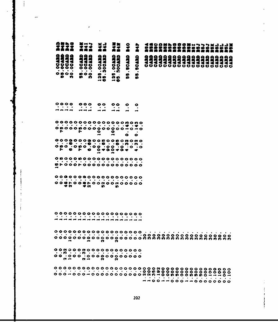
agil mom wes a a soamminamam
fil3 oil 11 111 1 ~awtmII swII w II 1990 000 00 00 0 0 0000000000000000o000000 0 00000 0..
0000 000 00 00 0 0
O0 0 000000000000n)01)
1-~ 0000600000000"00
010 010000*00 .0-.0
0000000000000oo0oooo
00..000E-0000000000000
cv C * qvkl o I
CO00OO0000000000000
00-000--~~4444--~-
-9 -e C C.4 C*
00000000lo0000000000oooooooooo00 .000000000000000000
CI.' Cl- Cl
--.00--0 -000000
202
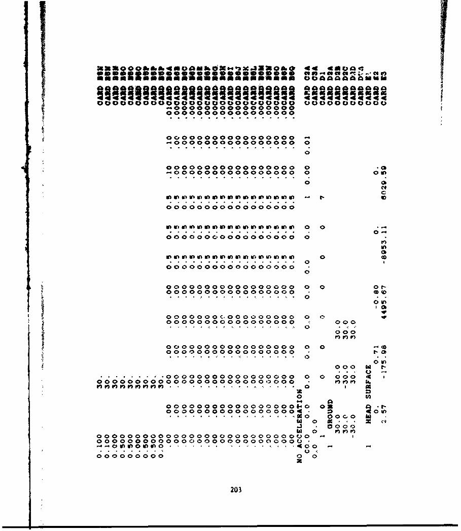
=3309 Q m i.&4%O4Mxom. 44 40004
Onomoo00404 biol
OUOOOOODOotjoO.)OrQC0p0 UOOOOODOOO40000000000000000
00000000000000000
g 00000000000000000-0000000000000000 0
0
00000000000000000 0 -0
-0000000000000000 0 OW1
C
. .. . . . . . . . . 0Of
000o000¢00000o00 0
U° * U ) M ° V* 0 0
* 04
00000000000000000
00000000000000000 0 0 or-00000000000000000 .(
0tr
0000000c,000000000 0 000000000000000000 . 000
i 000
00000000000000000 0 0 ]
00000000000000000000000000 t
oooo
000.00.0e00000000000000000 0 000000000000000000 o
. .0.0 . . . . . . . .. .. . . 0 0 0 C
Wa 0 ix * ..3* 0000lal 0 m )r
0000000000000 000000 000000000
000000 0 0
203
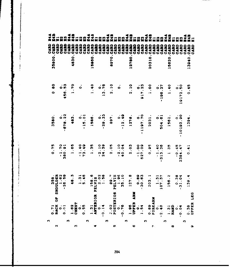
41 40 to 4a 40 4In 4
0~~- 0 0S)
o V1) 0 0 *0 0 0 *l0 *g- 0 *0 in0 00 1- 0 qr 0 r- -. 0 OC 0 Ol q* 00p q
o 0 ' I) C C . -0 - CI 0;
-4
0 0 f 1) 0 0 0 t 0 qv (4 0 - ow1 0 nb qo - -D - 0) t- r 0 -4 )
a w in In al OD -4C4 f 0I f
-4 0
In 0- i i 0 00 t 0 V 0 0 In 00 I f) 0 t-1- 1-0 o qv q nr - r 0 -0 0 00 ob r) r) r w 4
60 0~ 0N'I.n o t-( 41C
COI 0i ) -40 OCI 0 to0 40 40V ) r
IV) ~* W0 IV' (m (. n ct 00 0 t41 in o- r)(v WI r. a) ) -' r) Nl 0 '-
0 00 xa
03 0- 4 0to.. CI ) -4M -q C4 Q Oq. 40133w 0 .4 cor-ooo 0130 no 01001- 00.00 01640.' r) 0 0 r)A.
4 * - ' 0 * 010 -0 4-.00 0 -0 0 -4 0 'i ad 0 0 U O. Cl-E 0 0 :
204
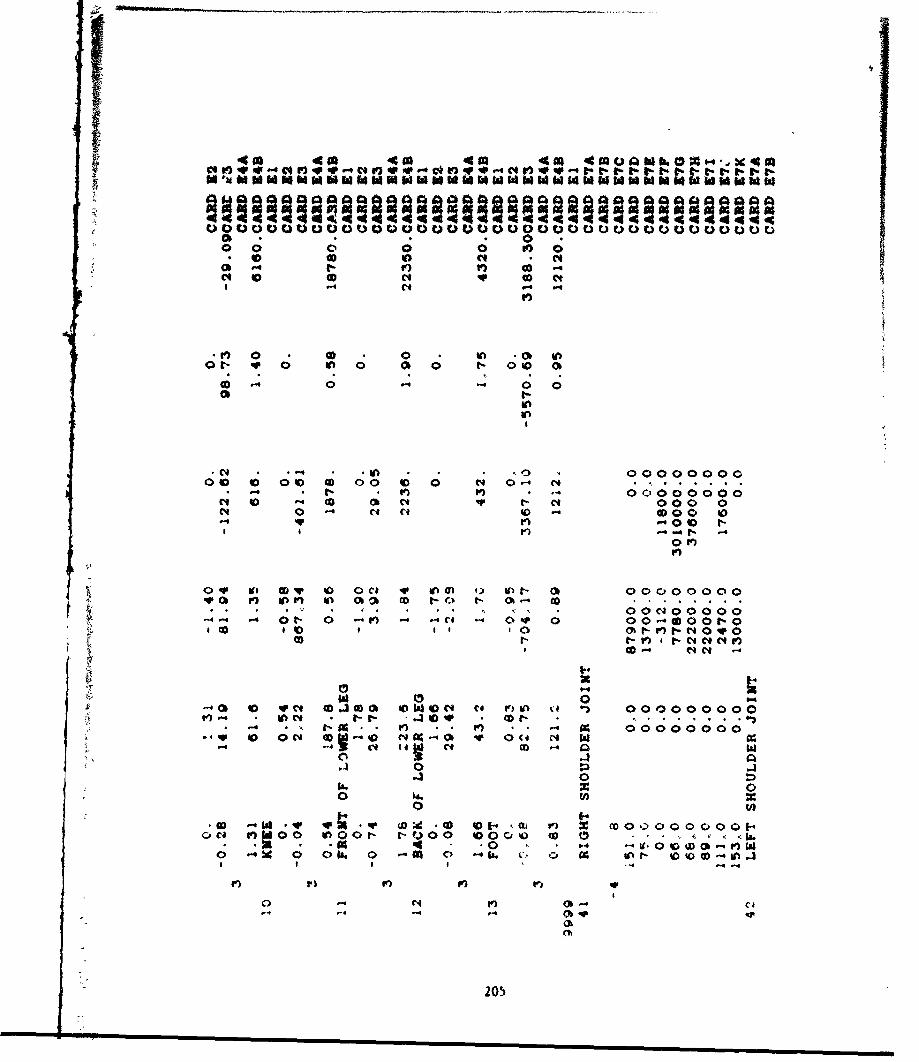
40 40 N 40 4o
P) 0 CD0i 0 b
0 " 0 0 000 ., 0o
* 0 0 0 C * o
V 00 0 0 0 0 0.
O .Q t to VC ) 00000000
N 0 * co 0 0 40 V * ..0 0 0 00
0 -. 0l -4"4 0
0~ r)
* --. in" o IV '0 0 0 0t-000
00 0 00 00 0 0 4000-i0
0 t, 0 a c0 000 0 t0OD 0#to 4 C) a 0 f0N0 00
'4~C (' N' ' 0 I
06'
04'4 a W 0C Ae OD 100)C C fr) n ( 000000000b ) CIO (40 4v (DC r- . .0
14 04' 0 00000i0to o I mI o0 C4 -weoC4 (-4
-4 V4 44 C4 4C0tg'
0 0
14 0 0
C)'A 0lo oC 0J tOW000 000% wa ( ) 0 00 0 044 .0 1 is '40 0 0 0 - W
-'4 x ON 010%4 0 M~~C 0 ' U (4 C, 1*) Of OG
-. 2 0
0 205
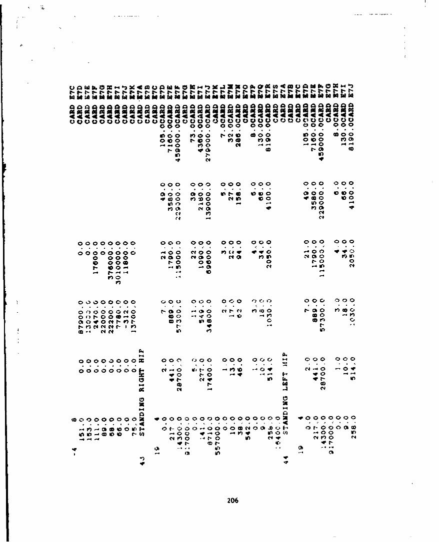
000 000 000 000 000 000. . . S *Sf <;
000 1 0 0 V) a o V)o ab0 0 10 74 0 Vq 0 cq -4 .4 40 q -. 4
000 000 000 000 000 000
0)00 0)00 0 el.0 @00 000 0 004 C40) 0 M D0 Clb In v 0 0 0
loo .40 .4(.lo 4
00000000 000 000 000 000 000 000
00000000 -.. 00 t4O 0 0 M(44. 4 q.0 -00 qv40 0~
0 000 N 0O 0O C) n 1-40 fl) 90 000 t. 0 00 0 10 0
I 00--0 -0C-0
00000000 000 00 00 0 000 OOC 000
o 0 0 C 0 r- Q0 -0)0 C -C r) ID0 t- 00 t)Wc0 1- 00 0 0 -r "0 0 '10
l-, CC'S 1" 0. 0 1t c ) pco0It- -r
t- 4
014
ooooa00ow 000 000 000 000 o 000 000
000O000 0 O C- 0 W - 0 0n 0-.4 (-l-o o
we. C4 0 f 4- 0
I- C4q4f
000000000A VOOO0000000000OOO2 VOOOoOO
-M 0 00 1 t-000-0000W100x f- or-oooow00-U)00 1-wi -00 4'".0 -V)4 1000 '-00 V)
C14 .-.- 0 0 to N. w NV)
t..
206
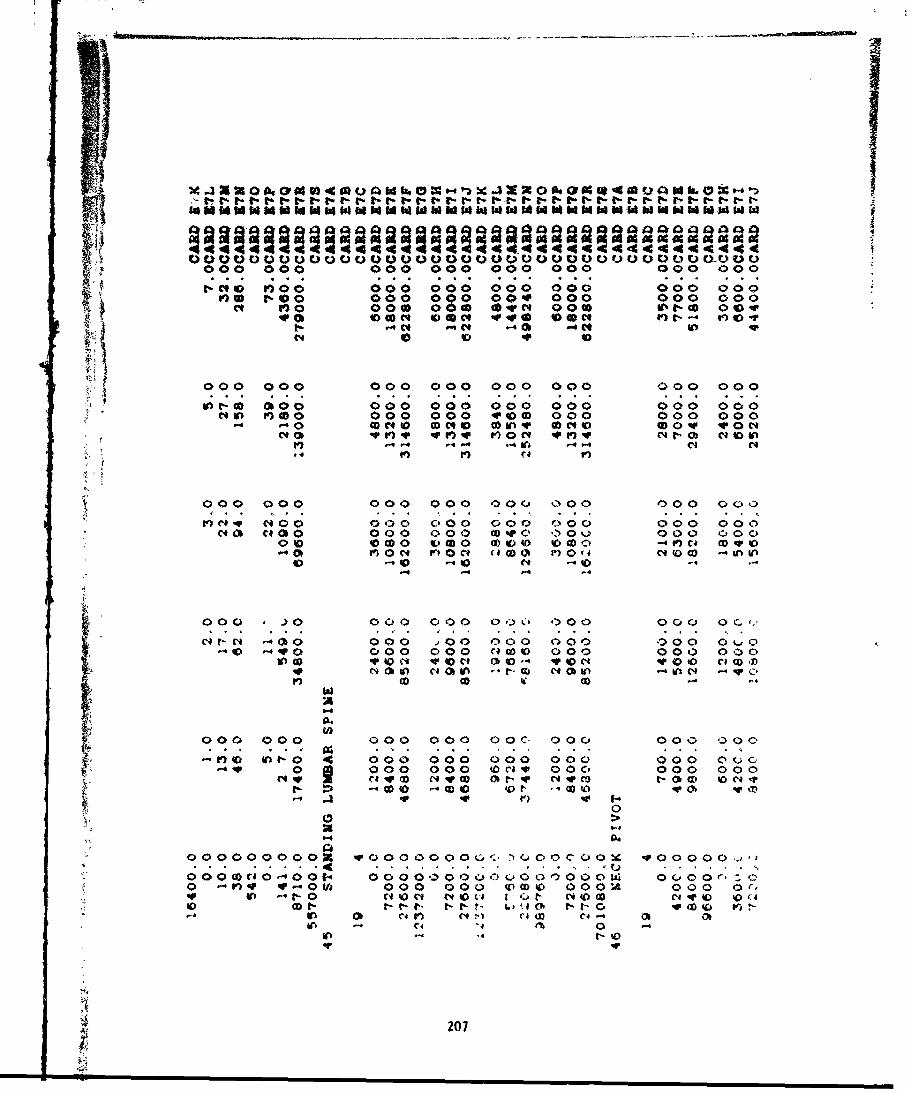
000 000 000 000 000 000 000 000
noI C%00 c00 000 000 000 000 000M) r00 000 0 ~0 OWN 000 000O 000
V4 O C'4 0" -W0 0Q4 C41
c~C If) 000 00 N 00 00I0 000
0010 000 000 000 000 000 000 000
00))00 000 000 00 t 000 000 000o
000~ 000 000 000 000 000 000 000
etb C GO 000 000 M~c W o30 000 000040 000 vM0 woo 000 - V) C4 Dw 00
0 m0 N 0 N' (100 P ( 0
000-' >~o 000 000 0 0 " 00 000 0tOCr- 0 40 00 000 C0 000 000 00
00D of0 000 000 c0 000 000 000In C-i)U AV40N v 0C4 0 v 40 N Via -0C' to C '4
I') 0) 0 0 1' 40 inN C
000 000 000 000 O0C. 000 000 -00
V; 4)0 t: 0 000 000 Q00 0 ;0 000 0 0co 0 000 000 0 N q 0 0c 000 000
4 W (A NVZ r IV wi~ coC 0 0 N
f- C 0f 'O 0 0F 1)00 vc
0
000000000~ V000000001 A'-000CQ0X V00000._,l
0 00 CV;040 01-4 0 C; 00o000, ,00 0 0Lao 0 -0 -no) W-0U) 000 000 '0wo 000o4 00o or,
o In -9- C4 0 clf N1 4_00( t" N~ fi)O CI NV o40 (D - t I'.f-i-. f- 611A h.Ch r- t-c CAV D 0
In4 ob CIO n I rio e (1 %
C4 0
207
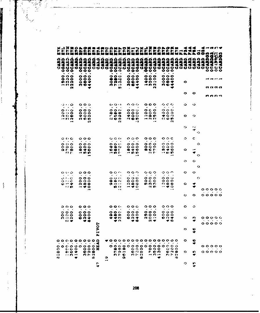
X~ -3X0O 004 0aN6 Xo-VmX0&W 4401
allV- I- .V* IA--bwI, $- p-IP. I V t a. * A r. .--- I00 000 00 000 00400
. . . . . . . . . . . . . .. . .
000 000 0 0 u 000 000 000000000 so,) 00 04 000
-'V)6 l 0 4ve (0.-.v 40co -If 09q)Ct V) 0 qv -O "ovCC
0 0
')'o 000 20) 0 <-( 000 O c'el: 0
O'*CP 000 0 OCA O0 .'p 0 cO 0 0 00<00 000 m0om 000 000 000NCA('0 '400c* r10 41V 90( C# M 0 n eS r 0 :D
r 4 es (** inc ) l 0i
,A
oclo 0 0 0 0j, 000 000 OO0c 0 C
0 c ;0 000 0 OF c 000 C 0 0 0 0000 000 -T ( fl 000 000 0 00
4l- C 0040 to004 440400 0 r- 0t 0 -
rae-- -'o in 0in -4010 ci- ut a( n-
0 C
00 000 00( C, oo 000 O0 0 0
Q'0 000 00'000 000 0 00,o'*C 000 43D( O 0 00 0 c0 00010" V CACDC -10 ~ - * (SOD n ~l 4 (ID0O 0 IV
'IV)~~~ -'9 0C -'4 0V C,0
0 0 00000
0030 000 o0( o0 000 000 0 0000 00 0 0oo ;C;C 00 000 0000c'0 000 040a) 000 000 000r)-. 0C4 N o994 r S ) 0 C4 V c 40 - 09)#O 0 V) 00000
1' 000000
94 IV
00C40000000 W0000000000000000 0000
o cCo 000w 000 000 00000
M( 1q 0 9 l CDf D0o) t 0 on 000
206
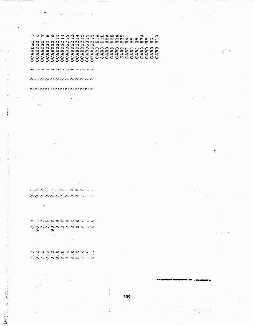
-4 -4 *.4 * - -4 -4 . -4 v ul 0 w t
II r.). ro r.) , I' r.) I') r),.) r') r) r 0i r. I r 1) .f r 2 r_ r z .
0000000000000 Utt0'0r)l)0000000
C14 cl cl i a- c cl aa C4 cla N el (1
D C)..) 0 0 0 p 000 ' ,,
i C) ") 000) 4)0E $, 20
;,i 209
Related Documents