Cycles and Instability in a Rock-Paper-Scissors Population Game: a Continuous Time Experiment * Timothy N. Cason † Purdue University Daniel Friedman ‡ UC Santa Cruz Ed Hopkins § University of Edinburgh July 19, 2012 Abstract We report laboratory experiments that use new, visually oriented software to ex- plore the dynamics of 3 × 3 games with intransitive best responses. Each moment, each player is matched against the entire population, here 8 human subjects. A “heat map” offers instantaneous feedback on current profit opportunities. In the continuous slow adjustment treatment, we see distinct cycles in the population mix. The cycle amplitude, frequency and direction are consistent with standard learning models. Cy- cles are more erratic and higher frequency in the instantaneous adjustment treatment. Control treatments (using simultaneous matching in discrete time) replicate previous results that exhibit weak or no cycles. Average play is approximated fairly well by Nash equilibrium, and an alternative point prediction, “TASP” (Time Average of the Shapley Polygon), captures some regularities that NE misses. JEL numbers: C72, C73, C92, D83 Keywords: experiments, learning, mixed equilibrium, continuous time. * We are grateful to the National Science Foundation for support under grant SES-0925039, and to Sam Wolpert and especially James Pettit for programming support, and Olga Rud, Justin Krieg and Daniel Nedelescu for research assistance. We received useful comments from audiences at the 2012 Contests, Mech- anisms & Experiments Conference at the University of Exeter; Purdue University; and the 2012 Economic Science Association International Conference at NYU. In particular, we want to thank Dieter Balkenborg, Dan Kovenock, Dan Levin, Eyal Winter and Zhijian Wang for helpful suggestions. † [email protected], http://www.krannert.purdue.edu/faculty/cason/ ‡ [email protected], http://leeps.ucsc.edu § [email protected], http://homepages.ed.ac.uk/hopkinse/

Welcome message from author
This document is posted to help you gain knowledge. Please leave a comment to let me know what you think about it! Share it to your friends and learn new things together.
Transcript

Cycles and Instability in a Rock-Paper-Scissors
Population Game: a Continuous Time Experiment∗
Timothy N. Cason†
Purdue University
Daniel Friedman‡
UC Santa Cruz
Ed Hopkins§
University of Edinburgh
July 19, 2012
Abstract
We report laboratory experiments that use new, visually oriented software to ex-
plore the dynamics of 3 × 3 games with intransitive best responses. Each moment,
each player is matched against the entire population, here 8 human subjects. A “heat
map” offers instantaneous feedback on current profit opportunities. In the continuous
slow adjustment treatment, we see distinct cycles in the population mix. The cycle
amplitude, frequency and direction are consistent with standard learning models. Cy-
cles are more erratic and higher frequency in the instantaneous adjustment treatment.
Control treatments (using simultaneous matching in discrete time) replicate previous
results that exhibit weak or no cycles. Average play is approximated fairly well by
Nash equilibrium, and an alternative point prediction, “TASP” (Time Average of the
Shapley Polygon), captures some regularities that NE misses.
JEL numbers: C72, C73, C92, D83
Keywords: experiments, learning, mixed equilibrium, continuous time.
∗We are grateful to the National Science Foundation for support under grant SES-0925039, and to Sam
Wolpert and especially James Pettit for programming support, and Olga Rud, Justin Krieg and Daniel
Nedelescu for research assistance. We received useful comments from audiences at the 2012 Contests, Mech-
anisms & Experiments Conference at the University of Exeter; Purdue University; and the 2012 Economic
Science Association International Conference at NYU. In particular, we want to thank Dieter Balkenborg,
Dan Kovenock, Dan Levin, Eyal Winter and Zhijian Wang for helpful suggestions.†[email protected], http://www.krannert.purdue.edu/faculty/cason/‡[email protected], http://leeps.ucsc.edu§[email protected], http://homepages.ed.ac.uk/hopkinse/

1 Introduction
Rock-Paper-Scissors, also known as RoShamBo, ShouShiLing (China) or JanKenPon (Japan)
is one of the world’s best known games. It may date back to the Han Dynasty 2000 years
ago, and in recent years has been featured in international tournaments for computerized
agents and humans (Fisher, 2008).
The game is iconic for game theorists, especially evolutionary game theorists, because it
provides the simplest example of intransitive dominance: strategy 1 (Rock) beats strategy
3 (Sissors) which beats strategy 2 (Paper), which beats strategy 1 (Rock). Evolutionary
dynamics therefore should be cyclic, possibly stable (and convergent to the mixed Nash
equilibrium), or perhaps unstable (and nonconvergent to any mixture). Questions regarding
cycles, stable or unstable, recur in more complex theoretical settings, and in applications
ranging from mating strategies for male lizards (Sinervo and Lively, 1996) to equilibrium
price dispersion with incomplete price information (e.g., Maskin and Tirole, 1988).
The present paper is an empirical investigation of behavior in RPS-like games, addressing
questions such as: Under what conditions does play converge to the unique interior NE? Or
to some other interior profile? Under what conditions do we observe cycles? If cycles
persist, does the amplitude converge to a maximal, minimal, or intermediate level? These
empirical questions spring from a larger question that motivates evolutionary game theory:
To understand strategic interaction, when do we need to go beyond equilibrium theory?
Surprisingly, we were able to find only two other human subject experiments investigat-
ing RPS-like games. Cason, Friedman, Hopkins (2010) study variations on a 4x4 symmetric
matrix game called RPSD, where the 4th strategy, D or Dumb, is never a best response.
Using the standard laboratory software zTree, the authors conducted 12 sessions, each with
12 subjects matched in randomly chosen pairs for 80 or more periods. In all treatments the
data were quite noisy, but in the most favorable condition (high payoffs and a theoretically
unstable matrix), the time-averaged data were slightly better explained by TASP (see section
2 below) than by Nash equilibrium. The paper reports no evidence of cycles.
Hoffman, Suetens, Nowak and Gneezy (2012) is another zTree study begun about the
same time as the present paper, and as far as we know, it is the only other human subject
experiment focusing on a RPS game. The authors compare behavior with three different sym-
1

metric 3x3 matrices of the form
0 −1 b
b 0 −1
−1 b 0
, where the treatments are b = 0.1, 1.0, 3.0.
The unique NE=(1,1,1)/3 is an ESS (hence in theory dynamically stable, see below) when
b = 3, but not in the other two treatments. The authors report 30 sessions each with 8
human subjects matched simultaneously with all others (mean-matching) for 100 periods.
They find that time average play is well approximated by NE, and that the mean distance
from NE is similar to that of binomial sampling error, except in the b = 0.1 treatment, when
the mean distance is larger. This paper also reports no evidence of cycles.
Section 2 reviews relevant theory and distills three testable hypotheses. Section 3 then
lays out our experimental design. The main innovations are (a) new visually-oriented soft-
ware called ConG, which enables players to choose mixed as well as pure strategies and to
adjust them in essentially continuous time, and (b) asymmetric 3x3 payoff bimatrices that
distinguish NE play from the centroid (1,1,1)/3. As in previous studies, we compare matrices
that are theoretically stable to those that are theoretically unstable, and in the latter case
we can distinguish TASP from NE as well as from the centroid. We also compare (virtually)
instantaneous adjustment to continuous but gradual adjustment (“Slow”), and to the more
familiar synchronized simultaneous adjustment in discrete time (“Discrete”).
Section 4 reports the results. After presenting graphs of average play over time in
sample periods and some summary statistics, it tests the three hypotheses. All three enjoy
considerable, but far from perfect, support. Among other things, we find that cycles persist
in the continuous time conditions in both the stable and unstable games, but that cycle
amplitudes are consistently larger in the unstable games. In terms of predicting time average
play, Nash equilibrium is better than Centroid, and when it differs from the NE, the TASP
is better yet.
A concluding discussion is followed by appendices that collect mathematical details and
instructions to subjects.
2

2 Some Theory
The games that were used in the experiments are, first, a game we call Ua
Ua =
R P S
Rock 60, 60 0, 72 66, 0
Paper 72, 0 60, 60 30, 72
Scissors 0, 66 72, 30 60, 60
(1)
where U is for unstable because, as we will show, many forms of learning will not converge
in this game. The subscript a distinguishes it from Ub that follows. Second, we have the
stable RPS game,
S =
R P S
Rock 36, 36 24, 96 66, 24
Paper 96, 24 36, 36 30, 96
Scissors 24, 66 96, 30 36, 36
(2)
Finally, we have a second unstable game Ub
Ub =
R P S
Rock 60, 60 72,0 30, 72
Paper 0, 72 60, 60 66, 0
Scissors 72, 30 0, 66 60, 60
(3)
Notice that in Ub the best response cycle is reversed so that it is a RSP game rather than
RPS.
All these games have the same unique Nash equilibrium which is mixed with probabilities
(0.25, 0.25, 0.5). The equilibrium payoff is 48 in all cases.
While these games are identical in their equilibrium predictions, they differ quite sub-
stantially in terms of predicted learning behavior. Consider as in our experiments a popula-
tion of players who play this game amongst themselves - one could consider either repeated
random matching or playing against the average mixed strategy of the other players. Sup-
pose they all choose a target for their mixed strategies that is (close to) a best response to
the current strategies of their opponents. Then the ConG software interface would adjust
their mixed strategies smoothly in that direction. Thus, we would expect that the pop-
ulation average mixed strategy x would move according to continuous time best response
3

(BR) dynamics, which assumes that the population average strategy moves smoothly in the
direction of the best reply to itself. That is, formally,
x ∈ b(x)− x (4)
where b(·) is the best response correspondence.1
Because of the cyclical nature of the best response structure of RPS games (Rock is
beaten by Paper which is beaten by Scissors which is beaten by Rock), if the evolution of
play can be approximated by the best response dynamics, then there will be cycles in play.
The question is whether these cycles converge or diverge.
It is easy to show that in the game S, under the best response dynamics, the average
strategy would converge to the Nash equilibrium. This is because the mixed equilibrium in
S is an evolutionarily stable strategy or ESS. In the games Ua and Ub, however, there will
be divergence from equilibrium and play will approach a limit cycle.2 For example, the case
of Ua is illustrated in Figure 1, with the interior triangle being the attracting cycle. This
cycle has been named a Shapley triangle or polygon after the work of Shapley (1964) who
was the first to produce an example of non-convergence of learning in games.
More recently, Benaım, Hofbauer and Hopkins (BHH) (2009) observe the following. If
play follows the BR dynamics then, in the unstable game, play will converge to the Shapley
triangle; furthermore, the time average of play will converge to a point that they name the
TASP (Time Average of the Shapley Polygon), denoted “T” on Figure 1. It is clearly distinct
from the Nash equilibrium of the game, denoted “N” in Figure 1.
These results can be stated formally in the following proposition. The proof can be
found in the Appendix.
Proposition 1 (a) The Nash equilibrium x∗ = (0.25, 0.25, 0.5) of the game Ua is unsta-
ble under the best response dynamics (4). Further, there is an attracting limit cycle, the
1Because this correspondence can be multivalued we use “∈”. However, for the RPS and RSP games we
consider the BR correspondence is single valued almost everywhere.2Intuitively, the instability arises in Ua and Ub because the normalized gain from winning (which ranges
from 6 to 12) is much smaller than the absolute normalized loss from losing (which ranges from -30 to -60).
By contrast, in the stable game S the normalized gain from winning (30 to 60) is much larger than the
absolute normalized loss from losing (-6 to -12). In other words, in the unstable games draws are almost as
good as wins, which pushes learning dynamics towards the corners of the simplex (see Figure 1 below) where
draws are more frequent. In the stable game draws are much worse than wins and only a little better than
losses, pushing the dynamics away from the corners and decreasing the amplitude of the cycles.
4

Figure 1: The Shapley triangle A1A2A3 for game Ua with the TASP (T) and the Nash equilibrium
(N). Also illustrated are orbits for the perturbed best response dynamics for precision parameter
values 0.2 and 0.5.
Shapley triangle, with vertices, A1 = (0.694, 0.028, 0.278), A2 = (0.156, 0.781, 0.063) and
A3 = (0.018, 0.089, 0.893) and time average, the TASP, of x ≈ (0.24, 0.31, 0.45). Average
payoffs on this cycle are approximately 51.1.
(b) The Nash equilibrium x∗ = (0.25, 0.25, 0.5) of the game S is a global attractor for the
best response dynamics (4).
(c) The Nash equilibrium x∗ = (0.25, 0.25, 0.5) of the game Ub is unstable under the best
response dynamics (4). Further, there is an attracting limit cycle, the Shapley triangle, with
vertices, A1 = (0.028, 0.694, 0.278), A2 = (0.781, 0.156, 0.063) and A3 = (0.089, 0.018, 0.893)
and time average, the TASP, of x ≈ (0.31, 0.24, 0.45). Average payoffs on this cycle are
approximately 51.1.
In the Appendix, we also outline the extent to which these results are robust to the possi-
bility of experiments and mistakes. Specifically, if subjects choose best responses imprecisely,
then average frequencies will evolve according to the perturbed best response (PBR) dynam-
ics rather than the strict BR dynamics. In games Ua and Ub, the PBR dynamics also give
rise to cycles, two of which for Ua are illustrated in Figure 1. How similar these are to the
Shapley cycle depends on the level of precision in subjects’ choices. See the Appendix for
5

details.
These theoretical arguments lead to the following testable predictions. Note that Hy-
pothesis 2 competes with Hypothesis 1, while Hypothesis 3(a) elaborates on Hypothesis 1
and Hypotheses 3(b,c,d) elaborate on Hypothesis 2.
Testable Hypotheses
1. Nash Equilibrium (NE): average play will be at the NE (0.25, 0.25, 0.5) and average
payoff will be 48 in all treatments.
2. TASP:
(a) The population average mixed strategy further averaged over time will be closer
to the TASP than to the NE in Ua and Ub.
(b) Average payoffs will be higher in Ua and Ub than in S.
3. BR Dynamics:
(a) In S, there will be counter-clockwise cycles that diminish in amplitude over time
with ultimate convergence to NE.
(b) In Ua, there will be persistent counter-clockwise cycles that approach the Shapley
triangle limit cycle.
(c) In Ub, there will be persistent clockwise cycles that approach the Shapley triangle
limit cycle.
(d) Thus the average distance from NE will be consistently higher in Ua and Ub than
in S.
3 Laboratory Procedures
Figure 2 displays an example of the subjects’ decision screen during an experimental session.
The upper left corner indicates the game payoff matrix M , and subjects choose actions by
clicking on locations on the “heat map” triangle in the lower left. They can choose a pure
action by clicking on a vertex, and can choose any desired mixture by clicking an interior
point. The thermometer to the right of the triangle shows how heat map colors correspond
6

Figure 2: ConG Software: CS treatment (10 sec transit)
to current payoff flow rates, given the current average mixture x(t) in the population. This
hugely reduces the subjects’ cognitive load, since otherwise they would continually have to
approximate, for each mixture y they might choose, the matrix product y ·Mx(t) that gives
the payoff flow.
The upper right side of the screen presents in real time the dynamic time path of
strategies selected by the subject and the population average. The lower right panel shows
the payoff flow received by the subject and the population average; the gray area represents
the player’s accumulated earnings so far in the current period.
Periods lasted 180 seconds each. Each session began with one unpaid practice period,
providing subjects with an opportunity to familiarize themselves with the interface and
display. The written instructions that were read aloud to subjects before this practice period
are included in Appendix B. Debriefings after the session was over, as well as experimenter
impressions during the session, indicate that most subjects quickly became comfortable with
the task, which they regarded as an enjoyable and not especially challenging video game.
Subjects participated in groups of 8 and played the three game matrices Ua, S and Ub
in treatment “blocks” of 5 periods each. Treatments were held constant within blocks, while
between blocks we switched the game matrix and changed the action set.
We used four different action sets: Continuous Instant, Continuous Slow, Discrete Pure
and Discrete Mixed. In the Continuous conditions, subjects click mixture targets and receive
payoff and population strategy updates in essentially continuous time. In the Instant case
7

the chosen mixture adjusted to their target click instantaneously; more precisely, lags are
typically less than 50 milliseconds, hence imperceptible. In the Slow case the actual mixture
moves at a constant rate towards the target click; the rate is such that it would take 10
seconds to move from one vertex to another.
In the Discrete conditions the 180-second period was subdivided into 20 subperiods of
9 seconds each, and subjects received payoff and population strategy updates at the end
of each subperiod. In the Pure case subjects were restricted to specify a pure strategy in
each subperiod, and in the Mixed case subjects could click any mixture or pure strategy in
each subperiod. (If the subject clicked several points during the subperiod, only the last
click counted.) Each subperiod after the first, the heat map displayed the potential payoffs
given the population mixture chosen in the previous subperiod, and therefore the heat map
remained static over the 9-second interval. In the Continuous conditions the heat map (and
the displays on the right side of the screen) updated every 200 milliseconds to reflect the
current population mixture.
Table 1: Balanced Incomplete Block Design
Block 1 Block 2 Block 3 Block 4 Block 5
Sess D1 Ua-DM S-CI Ua-DP S-DM Ub-CS
Sess D2 Ub-CS Ua-CS S-CS Ua-CI S-DP
Sess D3 S-CS Ua-DM S-CI Ub-CS S-DM
Sess D4 Ua-CI S-DM Ua-DM S-CS Ua-CI
Sess D5 S-DP Ub-CS Ua-DP S-CI Ua-CS
Sess D6 Ua-CS S-DP Ua-CI S-DM Ua-DP
Sess D7 S-CI Ua-CS Ub-CS S-CS Ua-DM
Sess D8 Ua-DP S-DM Ua-DM S-DP Ua-CI
Sess D9 S-CI Ua-DP S-DP Ua-CS S-CS
Sess D10 S-DM Ua-CI S-CS Ua-DP S-CI
Sess D11 Ua-CI S-DP Ua-CS Ub-CS Ua-DM
Note: Every treatment appears in Blocks 1 and 5, at least 8 out of 9 treatments appear
in each of the other Blocks, and no treatment appears more than twice in any Block.
Matrices Ua and S were played in each of the four action sets, while (as a bonus treat-
ment) Ub was played only in Continuous Slow. Thus we have 9 different combinations of
8

matrix and action set, or treatments. Each of the 11 sessions consisted of 5 blocks of 5
periods, with the treatment sequences shown in Table 1. The design was chosen to change
the matrix every block and to give 6 independent observations (i.e., from 6 different sessions)
of each of the 9 treatments, while balancing treatments across block positions.3
Each session lasted about 100 minutes, including instruction and payment time. No
subject participated in more than one session, and all were recruited broadly from the student
populations at Purdue University and UC-Santa Cruz. All 25 periods in the 5 blocks were
paid periods, and subject earnings averaged approximately $25.
4 Results
We begin with graphs of the population mixtures during some sample periods in the Con-
tinuous Slow treatment. The figures show a projection of the mixture triangle into the (x, y)
plane, so mixture probability for the third strategy (“Scissors”) is suppressed. The verti-
cal axis represents time remaining in the 180 second period, so moving downward in the
figure corresponds to moving forward in time. The NE appears as a vertical red line at
(x, y) = (.25, .25). The blue line in Figure 3 shows about a dozen irregular counterclockwise
cycles of the population average mix around the NE in a sample period using the stable S
matrix. Many of the cycles here have amplitude less than 0.1, but a few of them reach a
distance of 0.2 or more from the NE.
Figure 4 shows ten counterclockwise cycles around the NE for a sample period using
the unstable matrix Ua. The first few cycles (at the top) seem centered on the centroid
(x, y) = (0.33, 0.33) but last few cycles center closer to the NE. The amplitude is much
larger than for the S matrix, and falls only slightly by the end of the period. Figure 5 shows
11 cycles for the reverse unstable matrix Ub. They are similar to those for Ua, with one major
exception: as predicted, the cycles are clockwise.
These sample periods are typical in most respects. Time graphs for other periods suggest
that cycles in Continuous Slow treatments persist even with the stable matrix S, as well as
with (as predicted) the unstable matrices. The cycles typically seem to converge toward an
approximate limit cycle, rather than having inward or outward spirals. As we document
3One treatment Ua-CI was repeated in the final block of session D4, so it was excluded from the analysis
dataset because it is not statistically independent of the Ua-CI data in the first block of that session.
9

0.0 0.2 0.4 0.6 0.8 1.0
0 5
010
015
020
0
0.0
0.2
0.4
0.6
0.8
1.0
Tim
e R
emai
ning
Figure 3: Session 10, period 14: S matrix, Continuous-Slow.
0.0 0.2 0.4 0.6 0.8 1.0
0 5
010
015
020
0
0.0
0.2
0.4
0.6
0.8
1.0
Tim
e R
emai
ning
Figure 4: Session 2, period 6: Ua matrix,
Continuous-Slow.
0.0 0.2 0.4 0.6 0.8 1.0
0 5
010
015
020
0
0.0
0.2
0.4
0.6
0.8
1.0
Tim
e R
emai
ning
Figure 5: Session 11, period 20: Ub matrix,
Continuous-Slow.
10
0.0 0.2 0.4 0.6 0.8 1.0
60
70
80
90
100
110
120
0.0
0.2
0.4
0.6
0.8
1.0
Tim
e R
emai
ning
Figure 6: Session 3, period 14, Middle 1/3: S
matrix, Continuous-Instant.
0.0 0.2 0.4 0.6 0.8 1.0
60
70
80
90
100
110
120
0.0
0.2
0.4
0.6
0.8
1.0
Tim
e R
emai
ning
Figure 7: Session 2, period 17, Middle 1/3: Ua
matrix, Continuous-Instant.
below, consistent with Hypothesis 3abc, the cycles under Continuous Slow are consistently
counterclockwise for S and Ua and clockwise for Ub.
In the Instant treatment, the cycles are much more frequent and jagged, as Figures 6
and 7 illustrate, and also display greater amplitude for the Ua matrix. Note that only the
middle 60 seconds are shown, but even so there are more than a dozen cycles. In the Discrete
treatments, the path of population mixes by subperiod is not so obviously cyclic; see Figures
8 - 11 for typical examples.
4.1 Convergence across periods
Are there trends from one period to the next? To investigate, we plotted average population
mixtures in each of the 5 periods within each block separately for each treatment in each
session. The results for two of the treatments are displayed in Figures 12 and 13 for two of
the nine treatments.
Figure 12 shows that behavior remains quite unsettled in the treatment featured in
previous investigations — discrete time and pure strategy only — at least for the unstable
matrix Ua. For example, the population mean frequency of Scissors (shown in green) in one
11

0.0 0.2 0.4 0.6 0.8 1.0
0 5
010
015
020
0
0.0
0.2
0.4
0.6
0.8
1.0
Tim
e R
emai
ning
Figure 8: Session 3, period 24: S matrix,
Discrete-Mixed.
0.0 0.2 0.4 0.6 0.8 1.0
0 5
010
015
020
0
0.0
0.2
0.4
0.6
0.8
1.0
Tim
e R
emai
ning
Figure 9: Session 11, period 21: Ua matrix,
Discrete-Mixed.
0.0 0.2 0.4 0.6 0.8 1.0
0 5
010
015
020
0
0.0
0.2
0.4
0.6
0.8
1.0
Tim
e R
emai
ning
Figure 10: Session 2, period 22: S matrix,
Discrete-Pure
0.0 0.2 0.4 0.6 0.8 1.0
0 5
010
015
020
0
0.0
0.2
0.4
0.6
0.8
1.0
Tim
e R
emai
ning
Figure 11: Session 1, period 11: Ua matrix,
Discrete-Pure
12

0
0.1
0.2
0.3
0.4
0.5
0.6
0 1 2 3 4 5
Pro
por
tion
on
Str
ateg
y
Period within Block
Mean Strategy Choices: Unstable U3, Discrete Pure
Rock
Paper
Scissors
Figure 12: Mean choice by period within block
for the Ua matrix, Discrete-Pure treatment.
0
0.1
0.2
0.3
0.4
0.5
0.6
0 1 2 3 4 5
Pro
por
tion
on
Str
ateg
y
Period within Block
Mean Strategy Choices: Stable S3, Continuous Instant
Rock
Paper
Scissors
Figure 13: Mean choice by period within block
for the S matrix, Continuous-Instant treatment.
session bounces from about 0.26 in period 4 to 0.61 in period 5. Although Scissors seems the
most frequent strategy overall, and Rock (in blue) the least, this is reversed in some period
averages.
By contrast, Figure 13 shows very consistent mean strategy choices in the Continuous-
Instant treatment with the Stable matrix. The mean Rock frequency is always at or slightly
below the NE value of 0.25, and the Paper frequency at or slightly above. The mean Scissors
frequency is a bit below the NE value of 0.50 in period 1 but by period 5 clusters tightly
around that value. The other seven treatments show behavior more settled than in Figure
12 but less than in Figure 13.
4.2 Hypothesis Tests
Table 2 displays predicted (top 3 rows) and actual (remaining 9 rows) overall mean frequency
of each strategy and average payoffs. The superscripts refer to nonparametric Wilcoxon tests
that conservatively treat each session as a single independent observation. We draw the
following conclusions regarding the three testable Hypotheses given at the end of Section 2.
Result 1: In the Stable game, Nash Equilibrium is better than Centroid in predicting
13

time average strategy frequencies. Average payoff is significantly lower or not significantly
different than in Nash Equilibrium. Thus Hypothesis 1 finds mixed support.
Evidence: The N superscripts in Table 2 indicate that the data reject the Nash Equilib-
rium at the 5 percent significance level in 6 of the 12 strategy averages shown for the Stable
game. The centroid can be rejected in 11 out of these 12 cases for the Stable game S. (The
exception is Paper in the Discrete-Pure action set.) With only one other exception (again
Paper, here in Discrete-Mixed) the observed average strategy frequency is always closer to
NE than to the Centroid (1, 1, 1)/3. In each of the four treatments, the average payoff is
at least 1.3 below the Centroid payoff of 49.33. but it is always within 0.50 of the Nash
prediction of 48. The null hypothesis of Nash equilibrium payoffs is rejected (in favor of a
mean payoff lower than in NE) in two of these four treatments.
Table 2: Time average behavior
Prediction/Treatment Rock Paper Scissors Payoff
Nash Equilibrium 0.25 0.25 0.50 48
TASP (Ua) 0.242 0.31 0.449 51.1
TASP (Ub) 0.31 0.242 0.449 51.1
S Continuous-Instant 0.226N 0.269N 0.504 47.59N
S Continuous-Slow 0.236N 0.265 0.500 48.03
S Discrete-Mixed 0.242 0.294N 0.464 47.95
S Discrete-Pure 0.247 0.320N 0.433N 47.57N
Ua Continuous-Instant 0.247 0.318N 0.435N 49.82NT
Ua Continuous-Slow 0.228NT 0.281N 0.491T 49.08NT
Ua Discrete-Mixed 0.225 0.342NT 0.433N 49.70NT
Ua Discrete-Pure 0.205N 0.337N 0.458N 50.71N
Ub Continuous-Slow 0.303N 0.240 0.457N 48.81NT
Note: Superscript N denotes significantly different from Nash (5% 2-tailed Wilcoxon
test), and T denotes significantly different from TASP (5% 2-tailed Wilcoxon test;
conducted for Ua and Ub only).
Result 2: In the Unstable game, TASP is better than Nash Equilibrium (and a fortiori
better than Centroid) in predicting time average strategy frequencies. The average payoff
is always significantly higher than the Nash Equilibrium prediction and usually closer to
14

the TASP prediction, albeit significantly lower than the TASP prediction in most cases.
Moreover, consistent with TASP, payoffs are significantly higher in the Unstable game than
the Stable game. Thus Hypothesis 2 also finds mixed support.
Evidence: The N superscripts in Table 2 indicate rejection of the NE null hypothesis
in 11 of the 15 strategy frequencies for the Unstable game, and all rejections are in the
direction of TASP. Rejection the TASP predictions occurs in only 3 out of these 15 cases.
The average payoff always lies between the the NE and TASP predictions, but is closer
to TASP in 4 of 5 cases. In all 5 cases the Nash prediction of 48 is rejected; in one case
the TASP prediction is not rejected. In all 4 pairwise comparisons, average payoffs are
significantly higher (at the 1% level in Mann-Whitney tests) in the Unstable than the Stable
game. This is as predicted by TASP, while NE predicts no difference and Centroid predicts a
difference in the wrong direction. Finally, TASP tracks the observed asymmetry between Ua
and Ub in Rock and Paper time averages, while NE and Centroid predict no asymmetry. The
observed asymmetry (for their shared Continuous-Slow action set) is signficant according to
a Mann-Whitney test.
Result 3: Cycles are clockwise for the Unstable matrix Ub, and counter-clockwise for the
other matrices, Stable S and Unstable Ua. Although the cycle amplitudes usually decrease in
size across periods for the Stable matrix, they do not converge to Nash equilibrium, contrary
to Hypothesis 3a. Cycles also persist and have larger amplitudes for the Unstable matrices,
but less than that of the Shapley triangle limit cycle. Thus Hypotheses 3bc find mixed
support.
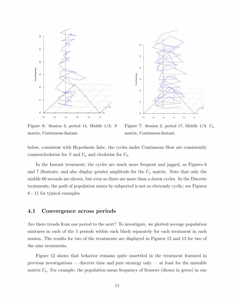
Evidence: Define cycle amplitude for a period as the time average over that period of the
squared Euclidean distance A(t) = ||x(t)−x∗||2 = (x0(t)−x∗0)2 +(x1(t)−x∗1)2 +(x2(t)−x∗2)2
between Nash equilibrium mix x∗ and the instantaneous actual mix x(t). (The average
squared deviation from the period average x yields similar results.) Figures 14 and 15
display cycle amplitude period by period for each block of the Continuous conditions; each
line comes from an independent session. The amplitude declines between the first and last
period in 22 out of the 24 blocks; the two exceptions are both in the Unstable - Continuous
Instant treatment. But the amplitudes do not decline to zero; even in later periods of the
12 Stable matrix blocks, the squared deviations remain around .01 (i.e., trajectories remain
about 0.10 away NE), contrary to Hypothesis 3a.
Table 3 reports average cycle amplitude in each treatment. Numerical calculations
indicate that the Shapley triangle limit cycle has amplitude 0.181 for the Ua and Ub matrices.
15
0
0.05
0.1
0.15
0.2
0.25
0 1 2 3 4 5
Squ
ared
Dev
iati
on f
rom
Nas
h E
qui
libri
um
Period within Block
Mean Squared Deviations from Nash, Continuous Instant
Unstable Matrix,Distance from Nash
Stable Matrix, Distancefrom Nash
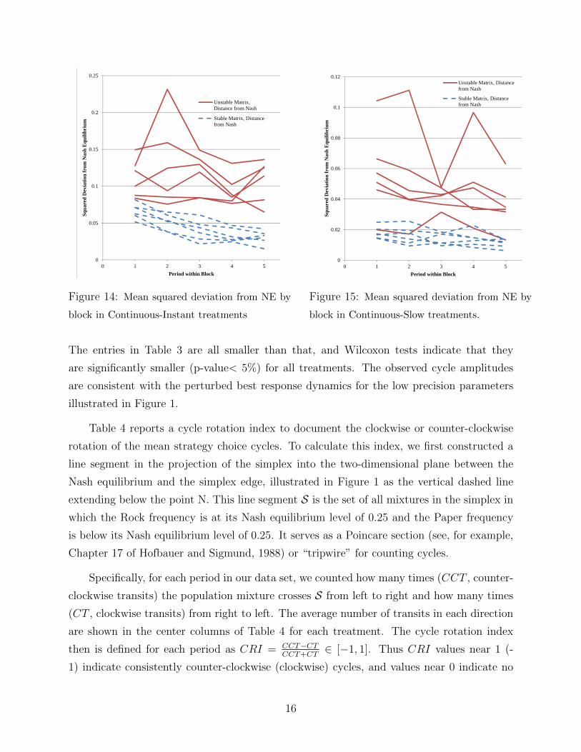
Figure 14: Mean squared deviation from NE by
block in Continuous-Instant treatments
0
0.02
0.04
0.06
0.08
0.1
0.12
0 1 2 3 4 5
Squa
red
Dev
iati
on f
rom
Nas
h E
quil
ibri
um
Period within Block
Mean Squared Deviations from Nash, Continuous Slow
Unstable Matrix, Distancefrom Nash
Stable Matrix, Distancefrom Nash
Figure 15: Mean squared deviation from NE by
block in Continuous-Slow treatments.
The entries in Table 3 are all smaller than that, and Wilcoxon tests indicate that they
are significantly smaller (p-value< 5%) for all treatments. The observed cycle amplitudes
are consistent with the perturbed best response dynamics for the low precision parameters
illustrated in Figure 1.
Table 4 reports a cycle rotation index to document the clockwise or counter-clockwise
rotation of the mean strategy choice cycles. To calculate this index, we first constructed a
line segment in the projection of the simplex into the two-dimensional plane between the
Nash equilibrium and the simplex edge, illustrated in Figure 1 as the vertical dashed line
extending below the point N. This line segment S is the set of all mixtures in the simplex in
which the Rock frequency is at its Nash equilibrium level of 0.25 and the Paper frequency
is below its Nash equilibrium level of 0.25. It serves as a Poincare section (see, for example,
Chapter 17 of Hofbauer and Sigmund, 1988) or “tripwire” for counting cycles.
Specifically, for each period in our data set, we counted how many times (CCT , counter-
clockwise transits) the population mixture crosses S from left to right and how many times
(CT , clockwise transits) from right to left. The average number of transits in each direction
are shown in the center columns of Table 4 for each treatment. The cycle rotation index
then is defined for each period as CRI = CCT−CTCCT+CT
∈ [−1, 1]. Thus CRI values near 1 (-
1) indicate consistently counter-clockwise (clockwise) cycles, and values near 0 indicate no
16

Table 3: Mean Squared Deviation from Nash Equilibrium
Continuous- Continuous- Discrete- Discrete-
Instant Slow Mixed Pure
Stable S 0.039 0.014 0.048 0.093
Unstable Ua 0.112 0.044 0.089 0.129
Unstable Ub 0.048
p-value for M-W: S vs. Ua 0.004 0.004 0.004 0.037
p-value for M-W: Ua vs. Ub 0.200
Notes: Excludes first period of each 5-period block to reduce impact of hysteresis. M-W is a
2-tailed Mann-Whitney test comparing MSDs by period across the given treatments.
consistent cycles. The last column of the Table reports CRI averaged over all periods in
each treatment.
The large values of CCT and CT the Continuous-Instant treatments reflect a substan-
tially higher cycle frequency than in the Continuous-Slow treaments. The Discrete treat-
ments have fewer transits, in part because each period has only 19 potential strategy changes,
versus 179 potential strategy changes each Continuous period, where the data are sampled
at one-second intervals.
The Discrete treatments for the Stable game S do not exhibit clear cyclical behavior, as
indicated by CRI’s not significantly different from 0. All other conditions exhibit significant
cycles, with only the Unstable game Ub displaying clockwise cycles, consistent with Hypoth-
esis 3abc. Although not shown on the table, Mann-Whitney tests with p-values below 0.05
for all four cases confirm that CRI always is larger for the Unstable matrix Ua than for the
Stable matrix S.
Result 4: Cycle amplitude, and thus average distance from the Nash Equilibrium, is
significantly higher in the Unstable than in the Stable game (support for Hypothesis 3d).
Evidence: The Mann-Whitney p-values shown at the bottom of Table 3 indicate that
the amplitude, conditioning on the action set condition, is always significantly greater in the
Unstable than the Stable game. The amplitude is not significantly different between the two
Unstable games for their shared Continuous-Slow action set, and no difference is expected
based on the hypotheses derived from BR dynamics.
17

Table 4: Mean Transits and Cycle Rotation Indexes
Game- Number of Counter- Number of Clockwise Cycle Rotation
Condition Clockwise Transits Transits Index
S Continuous-Instant 24.1 5.8 0.64*
S Continuous-Slow 9.3 0.9 0.86*
S Discrete-Mixed 2.1 1.3 0.30
S Discrete-Pure 0.5 0.7 -0.04
Ua Continuous-Instant 30.3 1.9 0.89*
Ua Continuous-Slow 8.3 0.0 1.00*
Ua Discrete-Mixed 1.8 0.3 0.78*
Ua Discrete-Pure 0.9 0.2 0.68*
Ub Continuous-Slow 0.3 8.5 -0.94*
Note: * Denotes Index significantly (p-value < 5%) different from 0 according to 2-tailed Wilcoxon test.
One loose end remains. What about cycle frequency, as opposed to cycle amplitude?
The last piece of evidence under Result 3 noted that the Unstable matrices produced more
consistent rotation direction directions than their Stable counterparts, but the CCT and
CT entries in Table 4 suggest no clear ordering on the number of cycles per period. Nor do
eyeball impressions of individual period graphs. We estimated cycle frequencies each period
using standard frequency domain techniques, employing the cumulative spectral distribution
function to identify the most significant cycle frequencies for the strategy and payoff time
series.4 Stronger cycles are evident in the continuous treatments, but overall the frequencies
are estimated with substantial noise. Nevertheless, tests show significantly higher frequencies
for the Ua-CI treatment than for Ua-CS, which comes as no surprise given the time series
graphs and the CCT and CT counts noted earlier. More importantly for present purposes,
we find no significant differences between S and Ua (or Ub) in any action treatment. This is
consistent with the Conjecture noted at the end of Appendix A.
4This procedure decomposes the time series into a weighted sum of sinusoidal functions to identify the
principal cycle frequencies.
18

5 Discussion
Evolutionary game theory predicts cyclic behavior in Rock-Paper-Scissors-like population
games, but such behavior has not been reported in previous work.5 In a continuous time
laboratory environment we indeed found cycles in population mixed strategies, most spectac-
ularly for the Unstable matrices with Slow adjustment. Moreover, we consistently observed
counterclockwise cycles for one Unstable matrix and clockwise cycles for another, just as
predicted.
Surprisingly, we also found very persistent cycles for Stable matrices, where the theory
predicted damped cycles and convergence to Nash Equilibrium. The theory was partially
vindicated in that these cycles had smaller amplitude than those for corresponding Unstable
matrices, but the amplitude settled down at a positive value, not at zero.
Evolutionary game theory considers several alternative dynamics. In our setting, repli-
cator dynamics predicts that the cycles for the Unstable matrices have maximal amplitude
(i.e., converge to the simplex boundary), while best response dynamics predict cycles that
converge to the Shapley triangle and therefore have a particular amplitude less than maxi-
mal. The amplitude of cycles we observed with Unstable matrices varied by the action set
available to each subject (instantaneous versus slow adjustment in continuous time, and pure
only versus mixed strategies in discrete time), but it was always less than for the Shapley
triangle. The data thus seem more consistent with perturbed best response dynamics with
treatment-dependent noise.
Classic game theory predicts that, on average, play will approximate Nash equilibrium.
Indeed, time averages over our three minute continuous time periods (and over 20 subperiod
discrete time periods) fairly closely approximated Nash equilibrium in all treatments. How-
ever, for the Unstable matrix, evolutionary game theory provides an alternative prediction
of central tendency called TASP, and it consistently outperformed Nash equilibrium.
Our results, therefore, are quite supportive of evolutionary game theory. It offers short
run predictions, where classic game theory has little to say, and those predictions for the
most part explained our data quite well. Its long run predictions either agreed with those of
classic game theory or else were more accurate in explaining our data.
5In laboratory studies focusing on convergence to mixed strategy equilibrium, Friedman (1996) and
Binmore et al (2001) both report some evidence of transient cyclic behavior in 2-population games. Neither
study considered RPS-like games or persistent cycles.
19

While seeking answers to old questions, our experiment also raises some new questions.
Granted that we observed very nice cyclic behavior, one now might want to know more about
the necessary conditions. Does our “heat map” play a crucial role? Or is asynchronous choice
in continuous time the key? Do cycles dissipate when subjects must choose simultaneously,
and some choose to best respond to the previous population mix while others respond to
their (“level k”) anticipations of others’ responses?
We hope our work inspires studies investigating such questions. It already seems clear
that empirically grounded learning models and evolutionary game dynamics can help us
grasp “instability,” an increasingly important theme for social scientists.
Appendix
In this appendix, we state and prove some results on the behavior of the best response (BR)
and perturbed best response (PBR) dynamics in the three games Ua, Ub and S.
When one considers stability of mixed equilibria under learning in a single, symmetric
population, the most general criterion for stability is negative definiteness of the game matrix,
which implies that a mixed equilibrium is an ESS (evolutionarily stable strategy). In contrast,
mixed equilibria in positive definite games are unstable. As Gaundersdorfer and Hofbauer
(1995) show, for RPS games there is a slightly weaker criterion for the stability/instability
of mixed equilibria under the BR dynamics (see below). The RPS games we consider satisfy
both criteria.
Proof of Proposition 1: Convergence to the Shapley triangle for the games Ua and Ub
follows directly from the results of Gaunersdorfer and Hofbauer (1995). In particular, first
one normalizes the payoff matrices by subtracting the diagonal payoff. Thus, for Ua, after
subtracting 60, the win payoffs become (12, 12, 6) and the lose payoffs in absolute terms
are (60, 60, 30). Thus clearly Ua satisfies the criterion (given in their Theorems 1 and 2)
for instability that the product of the lose payoffs is greater than the product of the win
payoffs.6 One can then calculate the Shapley triangle directly from their formula (3.6, p.
286). The TASP is calculated by the procedure given in Benaım, Hofbauer and Hopkins
(2009). The average payoff can similarly be calculated. These results are easily extended to
6Furthermore, Ua and UB are also positive definite with respect to the set IRn0 = {x ∈ IRn :
∑xi = 0}
which is a stronger criterion.
20

Ub.
Turning to S, subtracting 36, we find the win payoffs to be (60, 60, 30) and the lose
payoffs are (12, 12, 6). Thus, clearly the Nash equilibrium is globally stable because it
satisfies Gaundersdorfer and Hofbauer’s condition that the product of the win payoffs are
greater than the product of the lose payoffs.
We note that these results are largely robust to mistakes, particularly the possibility
that the choice of best response is not completely accurate. Suppose that subjects chose
a mixed strategy that is only an approximate best response to the current average mixed
strategy. Then we might expect that the population average might evolve according to the
perturbed best response dynamics
x = ψ(x)− x (5)
where the function ψ(·) is a perturbed choice function such as the logit.
Perturbed best response choice functions such as the logit are typically parameterized
with a precision parameter λ, which is the inverse of the amount of noise affecting the
individual’s choice. In such models, an increase of the precision parameter λ, for learning
outcomes are the following. First, it is well known that the stability of mixed equilibria under
the perturbed best response dynamics (5) depend upon the level of λ. When λ is very low,
agents randomize almost uniformly independently of the payoff structure and a perturbed
equilibrium close to the center of the simplex will be a global attractor. This means that
even in the unstable games Ua and Ub, the mixed equilibrium will only be unstable under
SFP if λ is sufficiently large. For the games Ua and Ub, it can be calculated that the critical
value of λ for the logit version of the dynamics is approximately 0.18. Second, in contrast,
in the stable game S, the mixed equilibrium will be stable independent of the value of λ.
Proposition 2 In Ua and Ub, the perturbed equilibrium (LE) x is unstable under the logit
form of the perturbed best response dynamics (5) for all λ > λ∗ ≈ 0.18. Further, at λ∗ there
is a supercritical Hopf bifurcation, so that for λ ∈ (λ∗, λ + ε) for some ε > 0, there is an
attracting limit cycle near x.
Proof: Instability follows from results of Hopkins (1999). The linearisation of the logit
PBR dynamics (5) at x will be of the form λR(x)B−I where R is the replicator operator and
B is the payoff matrix, either Ua or Ub. Its eigenvalues will therefore be of the form λki − 1
where the ki are the eigenvalues of R(x)B. R(x)B has only positive eigenvalues as both Ua
21

and Ub are positive definite. But for λ sufficiently small, all eigenvalues of λR(x)B − I will
be negative. We find the critical value of 0.18 by numerical analysis. The existence of a
supercritical Hopf bifurcation has been established by Hommes and Ochea (2012).
This result is less complete than Proposition 1, in that it does not give a complete
picture of PBR cycles away from equilibrium. Numeric analysis for the logit form of the
PBR dynamics suggests that as for the BR dynamics there is a unique attracting limit cycle
(for λ > 0.18). The amplitude of this cycle is increasing in λ and approaches that of the
Shapley triangle as λ becomes large. Two sample limit cycles are illustrated in Figure 1.
The game S is negative definite and hence its mixed equilibrium is a global attractor
under both the BR and PBR dynamics. This implies it is also an attractor for (stochastic)
fictitious play.
Proposition 3 The perturbed equilibrium (QRE) of the game S is globally asymptotically
stable under the perturbed best response dynamics (5) for all λ ≥ 0.
Proof: It is possible to verify that in the game S is negative definite with respect to
the set IRn0 = {x ∈ IRn :
∑xi = 0}. See e.g. Hofbauer and Sigmund (1998, p80) for the
negative definiteness (equivalently ESS) condition. The result then follows from Hofbauer
and Sandholm (2002).
Conjecture 1 For λ sufficiently large and for x sufficiently close to the perturbed equilibrium
x, cycles of the PBR dynamics, controlling for amplitude, should have the same frequency
for all three games Ua, Ub and S.
The reason behind the conjecture is the following. For λ large, the perturbed equilibrium
x is close to the NE x∗ = (1/4, 1/4, 1/2). It is then possible to approximate the PBR
dynamics by a linear system x = R(x∗)Bx where, for the logit version of the PBR dynamics,
R is the replicator operator (see the proof of Proposition 2 above) and B is the payoff matrix,
which could be any of Ua, Ub or S. One can calculate R(x∗)B, precisely for all three games
and thus derive the eigenvalues for this linear system, which are exactly 6 ± 9√
3i for Ua
and Ub and −6 ± 9√
3i for S. It is the imaginary part of the eigenvalues that determines
the frequency of the solutions of the linearized system x = R(x∗)Bx, while the exponent
of the real part determines the amplitude. The imaginary part is identical for all three
games and thus one would expect similar frequencies in cycles. Admittedly, there are two
22

approximations in making this argument. First, this is a linear approximation to the non-
linear PBR dynamics and will only be valid close to equilibrium. Second, the linearization
should properly be taken at x and not at the NE x∗. However, for λ large, the loss of
accuracy should not be too great.
References
Benaım, M., Hofbauer, J., and Hopkins, E. (2009). “Learning in games with unstable
equilibria”, Journal of Economic Theory, 144, 1694-1709.
Binmore, K., Swierzbinski, J. and Proulx, C. (2001). “Does Min-Max Work? An Experi-
mental Study,” Economic Journal, 111, 445-464.
Cason, T., Friedman, D. and Hopkins, E. (2010) “Testing the TASP: an Experimental
Investigation of Learning in Games with Unstable Equilibria”, Journal of Economic
Theory, November, 2010, 145, 2309-2331.
Fisher, Len (2008). Rock, paper, scissors: game theory in everyday life. Basic Books.
Friedman, D. (1996) “Equilibrium in Evolutionary Games: Some Experimental Results,”
Economic Journal, 106: 434, 1-25.
Gaunersdorfer, A., and J. Hofbauer (1995). “Fictitious play, Shapley Polygons, and the
Replicator Equation,” Games and Economic Behavior, 11, 279-303.
Hofbauer, J., Sigmund K., (1998) Evolutionary Games and Population Dynamics. Cam-
bridge: Cambridge University Press.
Hofbauer, J, W.H. Sandholm, (2002). “On the global convergence of stochastic fictitious
play”, Econometrica, 70, 2265-2294.
Hoffman, M., Suetens, S., Nowak, M., and Gneezy, U. (2011) “An experimental test of
Nash equilibrium versus evolutionary stability”, working paper.
Hommes, Cars H. and Marius I. Ochea (2012) “Multiple equilibria and limit cycles in
evolutionary games with Logit Dynamics”, Games and Economic Behavior, 74, 434-
441.
23

Hopkins, E. (1999). “A note on best response dynamics,” Games and Economic Behavior,
29, 138-150.
Maskin, E., and Tirole, J. (1988), “A Theory of Dynamic Oligopoly II: Price Competition,
Kinked Demand Curves, and Edgeworth Cycles, Econometrica, 56, 571-599.
Shapley, L. (1964). “Some topics in two person games,” in M. Dresher et al. eds., Advances
in Game Theory, Princeton: Princeton University Press.
Sinervo, B., and Lively, C. (1996). “The rock-paper-scissors game and the evolution of
alternative male strategies,” Nature, 380, 240 - 243.
24

UCSCLEEPSLAB February2012
AppendixB:ExperimentInstructions
Welcome!Thisisaneconomicsexperiment.Ifyoupaycloseattentiontotheseinstructions,youcanearnasignificantsumofmoney,whichwillbepaidtoyouincashattheendofthelastperiod.
Please remain silent and do not look at other participants’ screens. If you have anyquestions,orneedassistanceofanykind,pleaseraiseyourhandandwewillcometoyou.Ifyoudisrupttheexperimentbytalking,laughing,etc.,youmaybeaskedtoleaveandmaynotbepaid.Weexpectandappreciateyourcooperationtoday.
TheBasicIdea
Eachperiodyouwillbematchedanonymouslywithcounterparts,someoralloftheparticipantsintodaysexperiment.Youwillchoosemixturesofthreepossibleactions:A,BandC.Yourearningseachperiodwilldependonyourchoicesandthoseofyourcounterparts.Attheendofthesessionyourearningsinpointswillbeaddedupoverallperiods,convertedtoUSdollarsatarateshownonthewhiteboard,andpaidtoyouincash.
TheEarningsTable
Intheupperpartofthescreenyouwillseeatablewithrowslabeledbyyourchoice(A,BandC)andcolumnslabeledbythechoiceofyourcounterparts(a,bandc),asinFigure1.Eachtableentryrepresentsyourearningsgiventheindicatedchoices.Forexample,ifyouchooseactionAandthecounterpartschooseb,thenyourearningswillaccumulateatrate24,thenumbershowninrowAcolumnb.Theother8entriesinthetableshowyourearningsforallothercombinations.
MixturesandtheHeatMap
Insomeperiodstheexperimentgivesyoutheflexibilitytochoosemixturesofyourthreeactions.Tohelpyouseehowyourearningsdependonyourmixturechoiceandyourcounterparties’,yourcomputerscreenwillshowatriangular“heatmap”similartothatinFigure2.
The vertices in the triangle represent pure actions. That is, when you are at the vertexlabeledA,yourmixtureisof100%Aand0%BandC,whenatvertexCthenthemixtureisof100%actionCand0%AandB,similarlyforvertexB.Insomeperiodsyourchoicemayberestricted to thesevertices. Inotherperiods,youcanchooseanypoint in the triangleindicatingamixtureofactionsequaltotheproportionaldistancetoeachvertex.So,ifyouchoosetoplayinthemiddleofthetriangleyouwillbeplayingamixturewith33.33%A,33.33%Band33.33%C.InFigure2theblackdot(whichrepresentsyouractualmixtureofstrategies)isatis27%A,38%Band36%C. NotethatalongtheedgebetweenAandB,youarechoosing0%CandvaryingamixtureofonlyAandBactions,andthatpercentagesalwayshavetosumto100%(exceptforsmallroundingerrors).
Toadjustyourownmixture,clickyourmouseonthedesiredpoint.Thisbecomesthetargetandisdisplayedasacirclewithcrosshairs.Theblackdotwillmovesteadilytowardsyour

UCSCLEEPSLAB February2012
chosentarget.Insomeperiodsitmaymoveslowly,andinotherperiodsitmaymoveveryfast.Asmentioned,yourearningsrateisdeterminedbyyourmixtureandthatofthecounterparts’.Forexample,ifyourcounterpartschoose100%a,andyouchosethestrategyshowninFig2,thenyourearningsratewouldbe0.27(36)+0.38(96)+0.36(24)=54.84.Ifyourcounterpartschoseaninteriormixture,thenyourearningswouldbeaparticularweightedaverageofalltheentriesinthetable.
Sinceitishardtokeeptrackoftheseaveragesyourself,thecomputerwilluseacolorheatmaptohelpyou.Theredder(hotter)thecolor,thehigherwouldbeyourpayoffifyouweretochoosethatmixture;themoreviolet(colder)thecolorthelessthatchoicewouldpay.Athermometershowsthepayoffscaletotherightofthecoloredtriangle.InFigure2,theplayer’scurrentmixtureisinagreenish‐bluearea,receivingarateofpayof53.78.
Thesmallblacksquare(neartheBcornerinFigure2)showsthecounterparts’mixture,theaveragemixtureofallotherparticipantswithwhomyouarematched.Ascounterpartsadjusttheirmixtures,thesquarewillmove,andthatwillinturnchangetheheatmap.Themapalwaysshowsyourearningsrateatallofyourpossiblemixtures,giventhemixturecurrentlychosenbyyourcounterparts.
AccumulatedEarnings
Totherightofyourheatmapyouwillhaveadisplay(Figure3)showingyouraccumulatingearningsforthecurrentperiod.Yourearningsarerepresentedbythesolidgrayarea‐‐‐thelarger the area, the greater your accumulated earnings. The height of the gray linecorrespondstothecoloroftheheatmapwhereyourdotisatthatmoment.Sothehigherthegrayline,thefasteryourearningsareaccumulating.
The black line, with no solid area under it, represents the average earnings of yourcounterparts.Themoreareaundertheblackline,themoreyourcounterpartshaveearnedsofar.
Yourearningsattheendoftheperiodwilldependonthepercentageoftimeyouspendateach mixture combination. If, for example you spend half of the time in a mixturecombinationthatearnsyou10andhalfofthetimeinacombinationthatearnsyou20,thenyouwillearn(.5)10+(.5)20=15fortheperiod.
Itisimportanttorealizethatyourearningsdependnotonlyonthemixturecombination,but alsoonhowmuch timeyou andyour counterparts spend in the combination. If youspendallofyourtimeinonemixturecombination,thenyourpayofffortheperiodwillbetheareaunderaflatline.Ifeithermixturechanges,thenyouwillseethelinemoveupordown,andthegrayareaaccumulatingfasterorslower.
AsmalldisplaynearthetopofFigure4keepstrackofthemixesyouandyourcounterpartshavebeenplayingduringtheperiod.InthisdisplaythegraylineshowsthepercentageofAinyourmixateachpointintime,whiletheblacklineshowsyourcounterparts’percentageof action a. Similarly, the display shows the pastmixture of actions B and C during theperiod.

UCSCLEEPSLAB February2012
FullScreen
ThefullscreenyouwillseeduringtheexperimentwilllookliketheoneinFigure4.Itcontainstheearningstable,heatmap,theearningschart,andthemixturechart.
Theupperpartofthescreenshowsatimerthattellsyouhowmanysecondsareleftinthecurrentperiod.Rightbelowthetimerthescreenshowsyourearningssofarinthecurrentperiod,andthetotalearningsofthepreviousperiods.
Subperiods
Someperiodsmaybebrokendownintotwoormoresubperiods.Theyareshownasverticallinesinthepayoffdisplay,asinFigure5.
Whenyouseesubperiodlines,thismeansthatyourmixturechoicesmatteronlyattheendofeachsubperiod.Yourearningsfortheentiresubperiodarecomputedusingyourmixtureandthecounterparts’mixtureatthatpointoftime.Yourearningswillbeshownasusualasagrayareabelowaline.Thelineisautomaticallyflatineachsubperiod,sothegrayareawillliebelowanup‐and‐downstaircase.
Warning:duringeachsubperiod,theheatmapshowsthepayoffsthatwereavailabletoyouintheprevioussubperiod.Itcan’tshowthepayoffsthatactuallywillbeavailabletoyouthissubperiod,sinceyourcounterpartshavenotyetfinalizedtheirdecisions.
Earnings
Youwillbepaidattheendoftheexperimentforthetotalamountofpointsearnedoverallperiods,afteranyunpaidpracticeperiodsannouncedbytheconductor.TheconversionratefrompayoffpointstoUSdollarsiswrittenonthewhiteboard.

UCSCLEEPSLAB February2012
Frequentlyaskedquestions
Q1.Isthissomekindofpsychologicalexperimentwithanagendayouhaven'ttoldus?
Answer.No.Itisaneconomicsexperiment.Ifwedoanythingdeceptiveordon'tpayyoucashasdescribedthenyoucancomplaintothecampusHumanSubjectsCommitteeandwewillbeinserioustrouble.Theseinstructionsaremeanttoclarifyhowyouearnmoney;ourinterestissimplyinseeinghowpeoplemakedecisions.
Q2.Whatchangesfromoneperiodtothenext?
Answer.Thepayoffmatrixmightchange—besuretolookatit.Whenitdoes,ofcoursetheheatmapwilllookdifferently.Theadjustmentspeedmightalsobefasterorslowerthaninthepreviousperiod.Also,someperiodsmaybebrokendownintosubperiodsandinsomeperiodsyoumayonlybeabletochoosepureactionsonthethreevertices.Butoftennothingchangesbetweenperiods,andyouarematchedwithexactlythesamepeopleinexactlythesamewayasinthelastperiod.
Q3.Howistheaveragemixturedetermined?AmIpartofit?
Answer.Thecomputerlooksatthemixturescurrentlyusedbyeveryone,takesthesimpleaverage,andplotsitinthetriangle.Insomesessions,“everyone”meanseveryoneexceptyou,butinothersessionsitmeanseveryoneincludingyou.Theconductorwillwriteonthewhiteboardwhichwaythecomputerisdoingittoday.Usuallywehaveatleast8subjects,andtheaverageexceptyouisalmostthesameastheaverageincludingyou.
Q4.Iftheheatmapcolorlooksaboutthesameeverywhere,howcanItellwheremypayoffishighest?
Answer.Occasionallythismayhappen,anditmeansthatallmixturesgivealmostthesamepayoff.Evenwhenthecolorsarenotmuchofaclue,youcanalwaysrelyonthepayoffnumbersshownbymousingoverthemap;theyareaccuratetotwodecimalplaces.
Note:Ifyouarecolorblindtosomeorallthecolorsweuse,pleasementionthistotheexperimenterafteryouarepaid;itmayhelpusadjustthecolorschemelater.

UCSCLEEPSLAB February2012
Figure1
Figure2
Figure3

UCSCLEEPSLAB February2012
Figure4
Figure5
Related Documents