Cvpr13 Saliency

Saliency Detection via Graph-Based Manifold Ranking

Chuan Yang1, Lihe Zhang1, Huchuan Lu1, Xiang Ruan2, and Ming-Hsuan Yang3

1Dalian University of Technology 2OMRON Corporation 3University of California at Merced

Abstract

Most existing bottom-up methods measure the fore-ground saliency of a pixel or region based on its con-trast within a local context or the entire image, whereasa few methods focus on segmenting out background re-gions and thereby salient objects. Instead of consideringthe contrast between the salient objects and their surround-ing regions, we consider both foreground and backgroundcues in a different way. We rank the similarity of the im-age elements (pixels or regions) with foreground cues orbackground cues via graph-based manifold ranking. Thesaliency of the image elements is defined based on their rel-evances to the given seeds or queries. We represent theimage as a close-loop graph with superpixels as nodes.These nodes are ranked based on the similarity to back-ground and foreground queries, based on affinity matrices.Saliency detection is carried out in a two-stage scheme toextract background regions and foreground salient objectsefficiently. Experimental results on two large benchmarkdatabases demonstrate the proposed method performs wellwhen against the state-of-the-art methods in terms of ac-curacy and speed. We also create a more difficult bench-mark database containing 5,172 images to test the proposedsaliency model and make this database publicly availablewith this paper for further studies in the saliency field.

1. Introduction

The task of saliency detection is to identify the most im-portant and informative part of a scene. It has been appliedto numerous vision problems including image segmenta-tion [11], object recognition [28], image compression [16],content based image retrieval [8], to name a few. Saliencymethods in general can be categorized as either bottom-upor top-down approaches. Bottom-up methods [1, 2, 6, 7, 9–12, 14, 15, 17, 21, 24, 25, 27, 32, 33, 37] are data-driven andpre-attentive, while top-down methods [23, 36] are task-driven that entails supervised learning with class labels. Wenote that saliency models have been developed for eye fixa-tion prediction [6, 14, 15, 17, 19, 25, 33] and salient objectdetection [1, 2, 7, 9, 23, 24, 32]. The former focuses on

identifying a few human fixation locations on natural im-ages, which is important for understanding human attention.The latter is to accurately detect where the salient objectshould be, which is useful for many high-level vision tasks.In this paper, we focus on the bottom-up salient object de-tection tasks.

Salient object detection algorithms usually generatebounding boxes [7, 10], binary foreground and backgroundsegmentation [12, 23, 24, 32], or saliency maps which in-dicate the saliency likelihood of each pixel. Liu et al. [23]propose a binary saliency estimation model by training aconditional random field to combine a set of novel features.Wang et al. [32] analyze multiple cues in a unified energyminimization framework and use a graph-based saliencymodel [14] to detect salient objects. In [24] Lu et al. de-velop a hierarchical graph model and utilize concavity con-text to compute weights between nodes, from which thegraph is bi-partitioned for salient object detection. On theother hand, Achanta et al. [1] compute the saliency likeli-hood of each pixel based on its color contrast to the entireimage. Cheng et al. [9] consider the global region con-trast with respect to the entire image and spatial relation-ships across the regions to extract saliency map. In [11]Goferman et al. propose a context-aware saliency algo-rithm to detect the image regions that represent the scenebased on four principles of human visual attention. Thecontrast of the center and surround distribution of featuresis computed based on the Kullback-Leibler divergence forsalient object detection [21]. Xie et al. [35] propose a novelmodel for bottom-up saliency within the Bayesian frame-work by exploiting low and mid level cues. Sun et al. [30]improve the Xie’s model by introducing boundary and soft-segmentation. Recently, Perazzi et al. [27] show that thecomplete contrast and saliency estimation can be formu-lated in a unified way using high-dimensional Gaussian fil-ters. In this work, we generate a full-resolution saliencymap for each input image.

Most above-mentioned methods measure saliency bymeasuring local center-surround contrast and rarity of fea-tures over the entire image. In contrast, Gopalakrishnan etal. [12] formulate the object detection problem as a binarysegmentation or labelling task on a graph. The most salient

1

rank & inverse

×

×

×

binary

rank

input image

the first stage the second stage

get q

ueri

es

get queries

map

rank

side-specific mapfinal

queries

Figure 1. Diagram of our proposed model.

seed and several background seeds are identified by the be-havior of random walks on a complete graph and a k-regulargraph. Then, a semi-supervised learning technique is usedto infer the binary labels of the unlabelled nodes. Recently,a method that exploits background priors is proposed forsaliency detection [34]. The main observation is that thedistance between a pair of background regions is shorterthan that of a region from the salient object and a regionfrom the background. The node labelling task (either salientobject or background) is formulated as an energy minimiza-tion problem based on this criteria.

We observe that background often presents local orglobal appearance connectivity with each of four imageboundaries and foreground presents appearance coherenceand consistency. In this work, we exploit these cues to com-pute pixel saliency based on the ranking of superpixels. Foreach image, we construct a close-loop graph where eachnode is a superpixel. We model saliency detection as a man-ifold ranking problem and propose a two-stage scheme forgraph labelling. Figure 1 shows the main steps of the pro-posed algorithm. In the first stage, we exploit the boundaryprior [13, 22] by using the nodes on each side of image aslabelled background queries. From each labelled result, wecompute the saliency of nodes based on their relevances (i.e,ranking) to those queries as background labels. The four la-belled maps are then integrated to generate a saliency map.In the second stage, we apply binary segmentation on theresulted saliency map from the first stage, and take the la-belled foreground nodes as salient queries. The saliency ofeach node is computed based on its relevance to foregroundqueries for the final map.

To fully capture intrinsic graph structure information andincorporate local grouping cues in graph labelling, we usemanifold ranking techniques to learn a ranking function,which is essential to learn an optimal affinity matrix [20].Different from [12], the proposed saliency detection algo-

rithm with manifold ranking requires only seeds from oneclass, which are initialized with either the boundary pri-ors or foreground cues. The boundary priors are proposedinspired on the recent works of human fixations on im-ages [31], which shows that humans tend to gaze at the cen-ter of images. These priors have also been used in imagesegmentation and related problems [13, 22, 34]. In con-trast, the semi-supervised method [12] requires both back-ground and salient seeds, and generates a binary segmen-tation. Furthermore, it is difficult to determine the numberand locations of salient seeds as they are generated by ran-dom walks, especially for the scenes with different salientobjects. This is a known problem with graph labellingwhere the results are sensitive to the selected seeds. In thiswork, all the background and foreground seeds can be easilygenerated via background priors and ranking backgroundqueries (or seeds). As our model incorporates local group-ing cues extracted from the entire image, the proposed algo-rithm generates well-defined boundaries of salient objectsand uniformly highlights the whole salient regions. Exper-imental results using large benchmark data sets show thatthe proposed algorithm performs efficiently and favorablyagainst the state-of-the-art saliency detection methods.

2. Graph-Based Manifold Ranking

The graph-based ranking problem is described as fol-lows: given a node as a query, the remaining nodes areranked based on their relevances to the given query. Thegoal is to learn a ranking function, which defines the rele-vance between unlabelled nodes and queries.

2.1. Manifold Ranking

In [39], a ranking method that exploits the intrinsic man-ifold structure of data (such as image) for graph labellingis proposed. Given a dataset X =

{x1, . . . , xl, xl+1,

. . . , xn}∈ Rm×n, some data points are labelled queries

and the rest need to be ranked according to their relevancesto the queries. Let f : X → Rn denote a ranking func-tion which assigns a ranking value fi to each point xi,and f can be viewed as a vector f = [f1, . . . , fn]

T . Lety = [y1, y2, . . . , yn]

T denote an indication vector, in whichyi = 1 if xi is a query, and yi = 0 otherwise. Next, wedefine a graph G = (V,E) on the dataset, where the nodesV are the dataset X and the edges E are weighted by anaffinity matrix W = [wij ]n×n. Given G, the degree matrixis D = diag{d11, . . . , dnn}, where dii =

∑j wij . Similar

to the PageRank and spectral clustering algorithms [5, 26],the optimal ranking of queries are computed by solving thefollowing optimization problem:

2

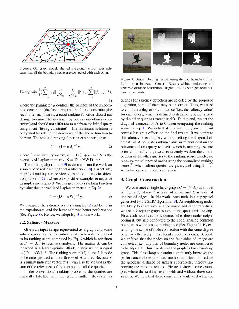
Figure 2. Our graph model. The red line along the four sides indi-cates that all the boundary nodes are connected with each other.

f∗=argminf

1

2(

n∑i,j=1

wij‖fi√dii− fj√

djj‖2+µ

n∑i=1

‖fi−yi‖2),

(1)where the parameter µ controls the balance of the smooth-ness constraint (the first term) and the fitting constraint (thesecond term). That is, a good ranking function should notchange too much between nearby points (smoothness con-straint) and should not differ too much from the initial queryassignment (fitting constraint). The minimum solution iscomputed by setting the derivative of the above function tobe zero. The resulted ranking function can be written as:

f∗ = (I− αS)−1y, (2)

where I is an identity matrix, α = 1/(1 + µ) and S is thenormalized Laplacian matrix, S = D−1/2WD−1/2.

The ranking algorithm [39] is derived from the work onsemi-supervised learning for classification [38]. Essentially,manifold ranking can be viewed as an one-class classifica-tion problem [29], where only positive examples or negativeexamples are required. We can get another ranking functionby using the unormalized Laplacian matrix in Eq. 2:

f∗ = (D− αW)−1y. (3)

We compare the saliency results using Eq. 2 and Eq. 3 inthe experiments, and the latter achieves better performance(See Figure 8). Hence, we adopt Eq. 3 in this work.

2.2. Saliency Measure

Given an input image represented as a graph and somesalient query nodes, the saliency of each node is definedas its ranking score computed by Eq. 3 which is rewrittenas f∗ = Ay to facilitate analysis. The matrix A can beregarded as a learnt optimal affinity matrix which is equalto (D − αW)−1. The ranking score f∗(i) of the i-th nodeis the inner product of the i-th row of A and y. Because yis a binary indicator vector, f∗(i) can also be viewed as thesum of the relevances of the i-th node to all the queries.

In the conventional ranking problems, the queries aremanually labelled with the ground-truth. However, as

Figure 3. Graph labelling results using the top boundary prior.Left: input images. Center: Results without enforcing thegeodesic distance constraints. Right: Results with geodesic dis-tance constraints.

queries for saliency detection are selected by the proposedalgorithm, some of them may be incorrect. Thus, we needto compute a degree of confidence (i.e., the saliency value)for each query, which is defined as its ranking score rankedby the other queries (except itself). To this end, we set thediagonal elements of A to 0 when computing the rankingscore by Eq. 3. We note that this seemingly insignificantprocess has great effects on the final results. If we computethe saliency of each query without setting the diagonal el-ements of A to 0, its ranking value in f∗ will contain therelevance of this query to itself, which is meaningless andoften abnormally large so as to severely weaken the contri-butions of the other queries to the ranking score. Lastly, wemeasure the saliency of nodes using the normalized rankingscore f

∗when salient queries are given, and using 1 − f

∗

when background queries are given.

3. Graph ConstructionWe construct a single layer graph G = (V,E) as shown

in Figure 2, where V is a set of nodes and E is a set ofundirected edges. In this work, each node is a superpixelgenerated by the SLIC algorithm [3]. As neighboring nodesare likely to share similar appearance and saliency values,we use a k-regular graph to exploit the spatial relationship.First, each node is not only connected to those nodes neigh-boring it, but also connected to the nodes sharing commonboundaries with its neighboring node (See Figure 2). By ex-tending the scope of node connection with the same degreeof k, we effectively utilize local smoothness cues. Second,we enforce that the nodes on the four sides of image areconnected, i.e., any pair of boundary nodes are consideredto be adjacent. Thus, we denote the graph as the close-loopgraph. This close-loop constraint significantly improves theperformance of the proposed method as it tends to reducethe geodesic distance of similar superpixels, thereby im-proving the ranking results. Figure 3 shows some exam-ples where the ranking results with and without these con-straints. We note that these constraints work well when the

3

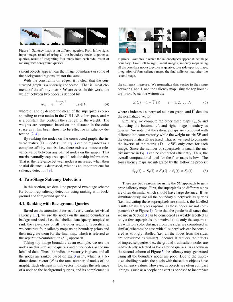
Figure 4. Saliency maps using different queries. From left to right:input image, result of using all the boundary nodes together asqueries, result of integrating four maps from each side, result ofranking with foreground queries.

salient objects appear near the image boundaries or some ofthe background regions are not the same.

With the constraints on edges, it is clear that the con-structed graph is a sparsely connected. That is, most ele-ments of the affinity matrix W are zero. In this work, theweight between two nodes is defined by

wij = e−‖ci−cj‖σ2 i, j ∈ V, (4)

where ci and cj denote the mean of the superpixels corre-sponding to two nodes in the CIE LAB color space, and σis a constant that controls the strength of the weight. Theweights are computed based on the distance in the colorspace as it has been shown to be effective in saliency de-tection [2, 4].

By ranking the nodes on the constructed graph, the in-verse matrix (D − αW)−1 in Eq. 3 can be regarded as acomplete affinity matrix, i.e., there exists a nonzero rele-vance value between any pair of nodes on the graph. Thismatrix naturally captures spatial relationship information.That is, the relevance between nodes is increased when theirspatial distance is decreased, which is an important cue forsaliency detection [9].

4. Two-Stage Saliency DetectionIn this section, we detail the proposed two-stage scheme

for bottom-up saliency detection using ranking with back-ground and foreground queries.

4.1. Ranking with Background Queries

Based on the attention theories of early works for visualsaliency [17], we use the nodes on the image boundary asbackground seeds, i.e., the labelled data (query samples) torank the relevances of all the other regions. Specifically,we construct four saliency maps using boundary priors andthen integrate them for the final map, which is referred asthe separation/combination (SC) approach.

Taking top image boundary as an example, we use thenodes on this side as the queries and other nodes as the un-labelled data. Thus, the indicator vector y is given, and allthe nodes are ranked based on Eq. 3 in f∗, which is a N -dimensional vector (N is the total number of nodes of thegraph). Each element in this vector indicates the relevanceof a node to the background queries, and its complement is

T

L

B

R

Figure 5. Examples in which the salient objects appear at the imageboundary. From left to right: input images, saliency maps usingall the boundary nodes together as queries, four side-specific maps,integration of four saliency maps, the final saliency map after thesecond stage.

the saliency measure. We normalize this vector to the rangebetween 0 and 1, and the saliency map using the top bound-ary prior, St can be written as:

St(i) = 1− f∗(i) i = 1, 2, . . . , N, (5)

where i indexes a superpixel node on graph, and f∗

denotesthe normalized vector.

Similarly, we compute the other three maps Sb, Sl andSr, using the bottom, left and right image boundary asqueries. We note that the saliency maps are computed withdifferent indicator vector y while the weight matrix W andthe degree matrix D are fixed. That is, we need to computethe inverse of the matrix (D − αW) only once for eachimage. Since the number of superpixels is small, the ma-trix inverse in Eq. 3 can be computed efficiently. Thus, theoverall computational load for the four maps is low. Thefour saliency maps are integrated by the following process:

Sbq(i) = St(i)× Sb(i)× Sl(i)× Sr(i). (6)

There are two reasons for using the SC approach to gen-erate saliency maps. First, the superpixels on different sidesare often disimilar which should have large distance. If wesimultaneously use all the boundary superpixels as queries(i.e., indicating these suprerpixels are similar), the labelledresults are usually less optimal as these nodes are not com-pactable (See Figure 4). Note that the geodesic distance thatwe use in Section 3 can be considered as weakly labelled asonly a few superpixels are involved (i.e., only the superpix-els with low color distance from the sides are considered assimilar) whereas the case with all superpixels can be consid-ered as strongly labelled (i.e., all the nodes from the sidesare considered as similar). Second, it reduces the effectsof imprecise queries, i.e., the ground-truth salient nodes areinadvertently selected as background queries. As shown inthe second column of Figure 5, the saliency maps generatedusing all the boundary nodes are poor. Due to the impre-cise labelling results, the pixels with the salient objects havelow saliency values. However, as objects are often compact“things” (such as a people or a car) as opposed to incompact

4

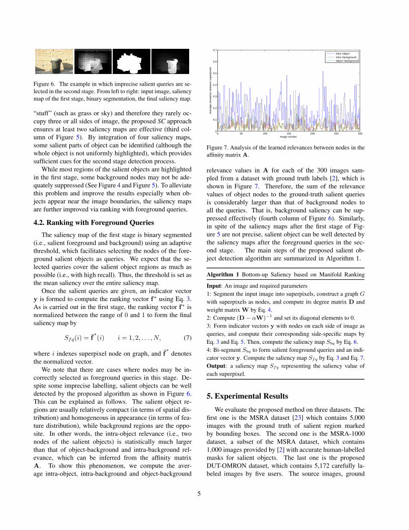
Figure 6. The example in which imprecise salient queries are se-lected in the second stage. From left to right: input image, saliencymap of the first stage, binary segmentation, the final saliency map.

“stuff” (such as grass or sky) and therefore they rarely oc-cupy three or all sides of image, the proposed SC approachensures at least two saliency maps are effective (third col-umn of Figure 5). By integration of four saliency maps,some salient parts of object can be identified (although thewhole object is not uniformly highlighted), which providessufficient cues for the second stage detection process.

While most regions of the salient objects are highlightedin the first stage, some background nodes may not be ade-quately suppressed (See Figure 4 and Figure 5). To alleviatethis problem and improve the results especially when ob-jects appear near the image boundaries, the saliency mapsare further improved via ranking with foreground queries.

4.2. Ranking with Foreground Queries

The saliency map of the first stage is binary segmented(i.e., salient foreground and background) using an adaptivethreshold, which facilitates selecting the nodes of the fore-ground salient objects as queries. We expect that the se-lected queries cover the salient object regions as much aspossible (i.e., with high recall). Thus, the threshold is set asthe mean saliency over the entire saliency map.

Once the salient queries are given, an indicator vectory is formed to compute the ranking vector f∗ using Eq. 3.As is carried out in the first stage, the ranking vector f∗ isnormalized between the range of 0 and 1 to form the finalsaliency map by

Sfq(i) = f∗(i) i = 1, 2, . . . , N, (7)

where i indexes superpixel node on graph, and f∗

denotesthe normalized vector.

We note that there are cases where nodes may be in-correctly selected as foreground queries in this stage. De-spite some imprecise labelling, salient objects can be welldetected by the proposed algorithm as shown in Figure 6.This can be explained as follows. The salient object re-gions are usually relatively compact (in terms of spatial dis-tribution) and homogeneous in appearance (in terms of fea-ture distribution), while background regions are the oppo-site. In other words, the intra-object relevance (i.e., twonodes of the salient objects) is statistically much largerthan that of object-background and intra-background rel-evance, which can be inferred from the affinity matrixA. To show this phenomenon, we compute the aver-age intra-object, intra-background and object-background

0 50 100 150 200 250 3000

0.1

0.2

0.3

0.4

0.5

0.6

0.7

Image number

Ave

rage

rev

elan

ce b

etw

een

supe

rpix

els

intra−objectintra−backgroundobject−background

Figure 7. Analysis of the learned relevances between nodes in theaffinity matrix A.

relevance values in A for each of the 300 images sam-pled from a dataset with ground truth labels [2], which isshown in Figure 7. Therefore, the sum of the relevancevalues of object nodes to the ground-truth salient queriesis considerably larger than that of background nodes toall the queries. That is, background saliency can be sup-pressed effectively (fourth column of Figure 6). Similarly,in spite of the saliency maps after the first stage of Fig-ure 5 are not precise, salient object can be well detected bythe saliency maps after the foreground queries in the sec-ond stage. The main steps of the proposed salient ob-ject detection algorithm are summarized in Algorithm 1.

Algorithm 1 Bottom-up Saliency based on Manifold Ranking

Input: An image and required parameters1: Segment the input image into superpixels, construct a graph Gwith superpixels as nodes, and compute its degree matrix D andweight matrix W by Eq. 4.2: Compute (D− αW)−1 and set its diagonal elements to 0.3: Form indicator vectors y with nodes on each side of image asqueries, and compute their corresponding side-specific maps byEq. 3 and Eq. 5. Then, compute the saliency map Sbq by Eq. 6.4: Bi-segment Sbq to form salient foreground queries and an indi-cator vector y. Compute the saliency map Sfq by Eq. 3 and Eq. 7.Output: a saliency map Sfq representing the saliency value ofeach superpixel.

5. Experimental Results

We evaluate the proposed method on three datasets. Thefirst one is the MSRA dataset [23] which contains 5,000images with the ground truth of salient region markedby bounding boxes. The second one is the MSRA-1000dataset, a subset of the MSRA dataset, which contains1,000 images provided by [2] with accurate human-labelledmasks for salient objects. The last one is the proposedDUT-OMRON dataset, which contains 5,172 carefully la-beled images by five users. The source images, ground

5

0 0.1 0.2 0.3 0.4 0.5 0.6 0.7 0.8 0.9 10

0.1

0.2

0.3

0.4

0.5

0.6

0.7

0.8

0.9

1

Recall

Pre

cisi

on

unnormalized Laplaican matrixnormalized Laplaican matrix

0 0.1 0.2 0.3 0.4 0.5 0.6 0.7 0.8 0.9 10

0.1

0.2

0.3

0.4

0.5

0.6

0.7

0.8

0.9

1

Recall

Pre

cisi

on

no close−loop constraint without k−regular graphclose−loop constraint with k−regular graphclose−loop constraint without k−regular graphno close−loop constraint with k−regular graph

0 0.1 0.2 0.3 0.4 0.5 0.6 0.7 0.8 0.9 10

0.1

0.2

0.3

0.4

0.5

0.6

0.7

0.8

0.9

1

Recall

Pre

cisi

on

using the SC approach with four boundary priorswithout using the SC approach

0 0.1 0.2 0.3 0.4 0.5 0.6 0.7 0.8 0.9 10

0.1

0.2

0.3

0.4

0.5

0.6

0.7

0.8

0.9

1

Recall

Pre

cisi

on

the first stagethe second stage

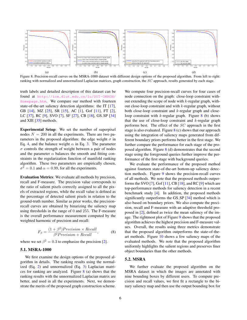
(a) (b) (c) (d)Figure 8. Precision-recall curves on the MSRA-1000 dataset with different design options of the proposed algorithm. From left to right:ranking with normalized and unnormalized Laplacian matrices, graph construction, the SC approach, results generated by each stage.

truth labels and detailed description of this dataset can befound at http://ice.dlut.edu.cn/lu/DUT-OMRON/

Homepage.htm. We compare our method with fourteenstate-of-the-art saliency detection algorithms: the IT [17],GB [14], MZ [25], SR [15], AC [1], Gof [11], FT [2],LC [37], RC [9], SVO [7], SF [27], CB [18], GS SP [34]and XIE [35] methods.

Experimental Setup: We set the number of superpixelnodes N = 200 in all the experiments. There are two pa-rameters in the proposed algorithm: the edge weight σ inEq. 4, and the balance weight α in Eq. 3. The parameterσ controls the strength of weight between a pair of nodesand the parameter α balances the smooth and fitting con-straints in the regularization function of manifold rankingalgorithm. These two parameters are empirically chosen,σ2 = 0.1 and α = 0.99, for all the experiments.

Evaluation Metrics: We evaluate all methods by precision,recall and F-measure. The precision value corresponds tothe ratio of salient pixels correctly assigned to all the pix-els of extracted regions, while the recall value is defined asthe percentage of detected salient pixels in relation to theground-truth number. Similar as prior works, the precision-recall curves are obtained by binarizing the saliency mapusing thresholds in the range of 0 and 255. The F-measureis the overall performance measurement computed by theweighted harmonic of precision and recall:

Fβ =(1 + β2)Precision×Recallβ2Precision+Recall

, (8)

where we set β2 = 0.3 to emphasize the precision [2].

5.1. MSRA-1000

We first examine the design options of the proposed al-gorithm in details. The ranking results using the normal-ized (Eq. 2) and unnormalized (Eq. 3) Laplacian matri-ces for ranking are analyzed. Figure 8 (a) shows that theranking results with the unnormalized Laplacian matrix arebetter, and used in all the experiments. Next, we demon-strate the merits of the proposed graph construction scheme.

We compute four precision-recall curves for four cases ofnode connection on the graph: close-loop constraint with-out extending the scope of node with k-regular graph, with-out close-loop constraint and with k-regular graph, withoutboth close-loop constraint and k-regular graph and close-loop constraint with k-regular graph. Figure 8 (b) showsthat the use of close-loop constraint and k-regular graphperforms best. The effect of the SC approach in the firststage is also evaluated. Figure 8 (c) shows that our approachusing the integration of saliency maps generated from dif-ferent boundary priors performs better in the first stage. Wefurther compare the performance for each stage of the pro-posed algorithm. Figure 8 (d) demonstrates that the secondstage using the foreground queries further improve the per-formance of the first stage with background queries.

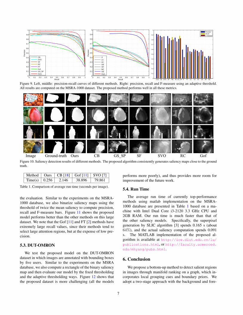
We evaluate the performance of the proposed methodagainst fourteen state-of-the-art bottom-up saliency detec-tion methods. Figure 9 shows the precision-recall curvesof all methods. We note that the proposed methods outper-forms the SVO [7], Gof [11], CB [18], and RC [9] which aretop-performance methods for saliency detection in a recentbenchmark study [4]. In addition, the proposed methodssignificantly outperforms the GS SP [34] method which isalso based on boundary priors. We also compute the preci-sion, recall and F-measure with an adaptive threshold pro-posed in [2], defined as twice the mean saliency of the im-age. The rightmost plot of Figure 9 shows that the proposedalgorithm achieves the highest precision and F-measure val-ues. Overall, the results using three metrics demonstratethat the proposed algorithm outperforms the state-of-the-art methods. Figure 10 shows a few saliency maps of theevaluated methods. We note that the proposed algorithmuniformly highlights the salient regions and preserves finerobject boundaries than the other methods.

5.2. MSRA

We further evaluate the proposed algorithm on theMSRA dataset in which the images are annotated withnine bounding boxes by different users. To compute pre-cision and recall values, we first fit a rectangle to the bi-nary saliency map and then use the output bounding box for

6

0 0.1 0.2 0.3 0.4 0.5 0.6 0.7 0.8 0.9 10

0.1

0.2

0.3

0.4

0.5

0.6

0.7

0.8

0.9

1

Recall

Pre

cisi

on

CB SVO SF RC FT Gof GS_SPOurs

0 0.1 0.2 0.3 0.4 0.5 0.6 0.7 0.8 0.9 10

0.1

0.2

0.3

0.4

0.5

0.6

0.7

0.8

0.9

1

Recall

Pre

cisi

on

IT LC AC GB SR MZ XIEOurs

Ours CB SVO SF XIE RC GS_SP IT FT LC CA AC GB SR MZ0

0.1

0.2

0.3

0.4

0.5

0.6

0.7

0.8

0.9

1

PrecisionRecallF−measure

Figure 9. Left, middle: precision-recall curves of different methods. Right: precision, recall and F-measure using an adaptive threshold.All results are computed on the MSRA-1000 dataset. The proposed method performs well in all these metrics.

Image Ground-truth Ours CB GS_SP SF SVO RC GofFigure 10. Saliency detection results of different methods. The proposed algorithm consistently generates saliency maps close to the groundtruth.

Method Ours CB [18] Gof [11] SVO [7]Time(s) 0.256 2.146 38.896 79.861

Table 1. Comparison of average run time (seconds per image).

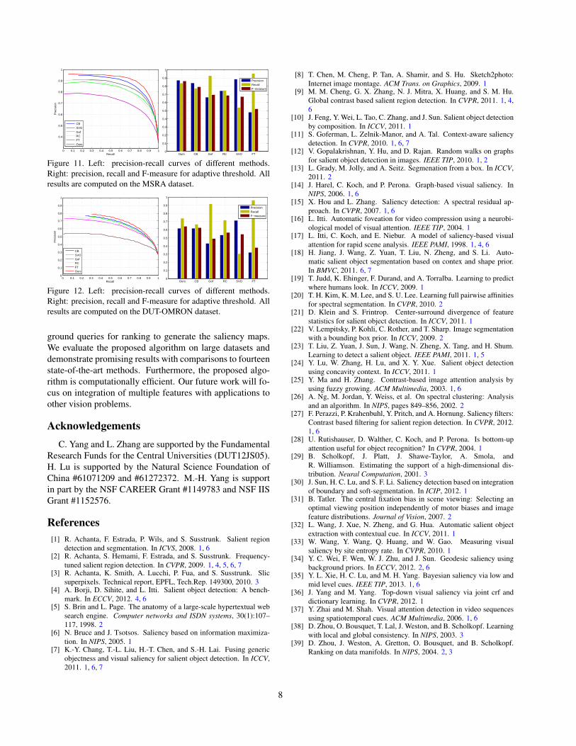
the evaluation. Similar to the experiments on the MSRA-1000 database, we also binarize saliency maps using thethreshold of twice the mean saliency to compute precision,recall and F-measure bars. Figure 11 shows the proposedmodel performs better than the other methods on this largedataset. We note that the Gof [11] and FT [2] methods haveextremely large recall values, since their methods tend toselect large attention regions, but at the expense of low pre-cision.

5.3. DUT-OMRON

We test the proposed model on the DUT-OMRONdataset in which images are annotated with bounding boxesby five users. Similar to the experiments on the MSRAdatabase, we also compute a rectangle of the binary saliencymap and then evaluate our model by the fixed thresholdingand the adaptive thresholding ways. Figure 12 shows thatthe proposed dataset is more challenging (all the models

performs more poorly), and thus provides more room forimprovement of the future work.

5.4. Run Time

The average run time of currently top-performancemethods using matlab implementation on the MSRA-1000 database are presented in Table 1 based on a ma-chine with Intel Dual Core i3-2120 3.3 GHz CPU and2GB RAM. Our run time is much faster than that ofthe other saliency models. Specifically, the superpixelgeneration by SLIC algorithm [3] spends 0.165 s (about64%), and the actual saliency computation spends 0.091s. The MATLAB implementation of the proposed al-gorithm is available at http://ice.dlut.edu.cn/lu/publications.html, or http://faculty.ucmerced.edu/mhyang/pubs.html.

6. Conclusion

We propose a bottom-up method to detect salient regionsin images through manifold ranking on a graph, which in-corporates local grouping cues and boundary priors. Weadopt a two-stage approach with the background and fore-

7

0 0.1 0.2 0.3 0.4 0.5 0.6 0.7 0.8 0.9 1

0.4

0.5

0.6

0.7

0.8

0.9

1

Recall

Pre

cisi

on

CBSVOGofRCFTOurs

Ours CB Gof RC SVO FT0

0.1

0.2

0.3

0.4

0.5

0.6

0.7

0.8

0.9

1

PrecisionRecallF−measure

Figure 11. Left: precision-recall curves of different methods.Right: precision, recall and F-measure for adaptive threshold. Allresults are computed on the MSRA dataset.

0 0.1 0.2 0.3 0.4 0.5 0.6 0.7 0.8 0.9 10

0.1

0.2

0.3

0.4

0.5

0.6

0.7

0.8

0.9

1

Recall

Pre

cisi

on

CBSVOGofRCFTOurs

Ours CB Gof RC SVO FT0

0.1

0.2

0.3

0.4

0.5

0.6

0.7

0.8

0.9

1

PrecisionRecallF−measure

Figure 12. Left: precision-recall curves of different methods.Right: precision, recall and F-measure for adaptive threshold. Allresults are computed on the DUT-OMRON dataset.

ground queries for ranking to generate the saliency maps.We evaluate the proposed algorithm on large datasets anddemonstrate promising results with comparisons to fourteenstate-of-the-art methods. Furthermore, the proposed algo-rithm is computationally efficient. Our future work will fo-cus on integration of multiple features with applications toother vision problems.

AcknowledgementsC. Yang and L. Zhang are supported by the Fundamental

Research Funds for the Central Universities (DUT12JS05).H. Lu is supported by the Natural Science Foundation ofChina #61071209 and #61272372. M.-H. Yang is supportin part by the NSF CAREER Grant #1149783 and NSF IISGrant #1152576.

References[1] R. Achanta, F. Estrada, P. Wils, and S. Susstrunk. Salient region

detection and segmentation. In ICVS, 2008. 1, 6[2] R. Achanta, S. Hemami, F. Estrada, and S. Susstrunk. Frequency-

tuned salient region detection. In CVPR, 2009. 1, 4, 5, 6, 7[3] R. Achanta, K. Smith, A. Lucchi, P. Fua, and S. Susstrunk. Slic

superpixels. Technical report, EPFL, Tech.Rep. 149300, 2010. 3[4] A. Borji, D. Sihite, and L. Itti. Salient object detection: A bench-

mark. In ECCV, 2012. 4, 6[5] S. Brin and L. Page. The anatomy of a large-scale hypertextual web

search engine. Computer networks and ISDN systems, 30(1):107–117, 1998. 2

[6] N. Bruce and J. Tsotsos. Saliency based on information maximiza-tion. In NIPS, 2005. 1

[7] K.-Y. Chang, T.-L. Liu, H.-T. Chen, and S.-H. Lai. Fusing genericobjectness and visual saliency for salient object detection. In ICCV,2011. 1, 6, 7

[8] T. Chen, M. Cheng, P. Tan, A. Shamir, and S. Hu. Sketch2photo:Internet image montage. ACM Trans. on Graphics, 2009. 1

[9] M. M. Cheng, G. X. Zhang, N. J. Mitra, X. Huang, and S. M. Hu.Global contrast based salient region detection. In CVPR, 2011. 1, 4,6

[10] J. Feng, Y. Wei, L. Tao, C. Zhang, and J. Sun. Salient object detectionby composition. In ICCV, 2011. 1

[11] S. Goferman, L. Zelnik-Manor, and A. Tal. Context-aware saliencydetection. In CVPR, 2010. 1, 6, 7

[12] V. Gopalakrishnan, Y. Hu, and D. Rajan. Random walks on graphsfor salient object detection in images. IEEE TIP, 2010. 1, 2

[13] L. Grady, M. Jolly, and A. Seitz. Segmenation from a box. In ICCV,2011. 2

[14] J. Harel, C. Koch, and P. Perona. Graph-based visual saliency. InNIPS, 2006. 1, 6

[15] X. Hou and L. Zhang. Saliency detection: A spectral residual ap-proach. In CVPR, 2007. 1, 6

[16] L. Itti. Automatic foveation for video compression using a neurobi-ological model of visual attention. IEEE TIP, 2004. 1

[17] L. Itti, C. Koch, and E. Niebur. A model of saliency-based visualattention for rapid scene analysis. IEEE PAMI, 1998. 1, 4, 6

[18] H. Jiang, J. Wang, Z. Yuan, T. Liu, N. Zheng, and S. Li. Auto-matic salient object segmentation based on contex and shape prior.In BMVC, 2011. 6, 7

[19] T. Judd, K. Ehinger, F. Durand, and A. Torralba. Learning to predictwhere humans look. In ICCV, 2009. 1

[20] T. H. Kim, K. M. Lee, and S. U. Lee. Learning full pairwise affinitiesfor spectral segmentation. In CVPR, 2010. 2

[21] D. Klein and S. Frintrop. Center-surround divergence of featurestatistics for salient object detection. In ICCV, 2011. 1

[22] V. Lempitsky, P. Kohli, C. Rother, and T. Sharp. Image segmentationwith a bounding box prior. In ICCV, 2009. 2

[23] T. Liu, Z. Yuan, J. Sun, J. Wang, N. Zheng, X. Tang, and H. Shum.Learning to detect a salient object. IEEE PAMI, 2011. 1, 5

[24] Y. Lu, W. Zhang, H. Lu, and X. Y. Xue. Salient object detectionusing concavity context. In ICCV, 2011. 1

[25] Y. Ma and H. Zhang. Contrast-based image attention analysis byusing fuzzy growing. ACM Multimedia, 2003. 1, 6

[26] A. Ng, M. Jordan, Y. Weiss, et al. On spectral clustering: Analysisand an algorithm. In NIPS, pages 849–856, 2002. 2

[27] F. Perazzi, P. Krahenbuhl, Y. Pritch, and A. Hornung. Saliency filters:Contrast based filtering for salient region detection. In CVPR, 2012.1, 6

[28] U. Rutishauser, D. Walther, C. Koch, and P. Perona. Is bottom-upattention useful for object recognition? In CVPR, 2004. 1

[29] B. Scholkopf, J. Platt, J. Shawe-Taylor, A. Smola, andR. Williamson. Estimating the support of a high-dimensional dis-tribution. Neural Computation, 2001. 3

[30] J. Sun, H. C. Lu, and S. F. Li. Saliency detection based on integrationof boundary and soft-segmentation. In ICIP, 2012. 1

[31] B. Tatler. The central fixation bias in scene viewing: Selecting anoptimal viewing position independently of motor biases and imagefeature distributions. Journal of Vision, 2007. 2

[32] L. Wang, J. Xue, N. Zheng, and G. Hua. Automatic salient objectextraction with contextual cue. In ICCV, 2011. 1

[33] W. Wang, Y. Wang, Q. Huang, and W. Gao. Measuring visualsaliency by site entropy rate. In CVPR, 2010. 1

[34] Y. C. Wei, F. Wen, W. J. Zhu, and J. Sun. Geodesic saliency usingbackground priors. In ECCV, 2012. 2, 6

[35] Y. L. Xie, H. C. Lu, and M. H. Yang. Bayesian saliency via low andmid level cues. IEEE TIP, 2013. 1, 6

[36] J. Yang and M. Yang. Top-down visual saliency via joint crf anddictionary learning. In CVPR, 2012. 1

[37] Y. Zhai and M. Shah. Visual attention detection in video sequencesusing spatiotemporal cues. ACM Multimedia, 2006. 1, 6

[38] D. Zhou, O. Bousquet, T. Lal, J. Weston, and B. Scholkopf. Learningwith local and global consistency. In NIPS, 2003. 3

[39] D. Zhou, J. Weston, A. Gretton, O. Bousquet, and B. Scholkopf.Ranking on data manifolds. In NIPS, 2004. 2, 3

8