Cutting Rules at Finite Temperature

arX

iv:h

ep-p

h/96

0332

5v1

15

Mar

199

6

MIT-CTP-2490

UR-1447

MRI-Phy-95-26

hep-ph/9603325

CUTTING RULES AT FINITE TEMPERATURE

Paulo F. Bedaque∗

Center for Theoretical PhysicsLaboratory for Nuclear Science

and Department of PhysicsMassachusetts Institute of Technology

Cambridge, Massachusetts 02139

Ashok Das

Department of Physics and AstronomyUniversity of RochesterRochester, N.Y. 14627

Satchidananda Naik†

Mehta Research Institute of Mathematicsand Mathematical Physics10, Kasturba Gandhi MargAllahabad 211002, India

( February 1996)

Abstract

We discuss the cutting rules in the real time approach to finite temperature field theoryand show the existence of cancellations among classes of cut graphs which allows a physicalinterpretation of the imaginary part of the relevant amplitude in terms of underlying micro-scopic processes. Furthermore, with these cancellations, any calculation of the imaginarypart of an amplitude becomes much easier and completely parallel to the zero temperaturecase.

∗Email address: [email protected]

†Email address: [email protected]

I. INTRODUCTION

At zero temperature, the evaluation of the imaginary part of a scattering amplitude isimmensely simplified by the use of the cutting (Cutkosky) rules [1] which further make theunitarity of the S-matrix manifest. The fact that the imaginary part of a n-loop amplitudecan be related to the on-shell amplitudes with lower order loops is best seen, in the modernlanguage, by the use of the so called largest time equation of ’t Hooft and Veltman [2].Generalizations of these rules to the finite temperature case are essential and useful since alarge number of transport coefficients are given by the imaginary part of some equilibriumfinite temperature correlators. The cutting rules at finite temperature will not only simplifythe evaluation of these coefficients but will also help in understanding the structure of fieldtheories at finite temperature as well as identifying the microscopic processes underlyingthem. In this paper, we provide such a generalization in the real time approach to finitetemperature field theories.

Finite temperature (and density) extensions of the cutting rules have been discussed, inthe past, both in the imaginary time formalism [3] as well as in the real time formalism [4].Explicit imaginary time calculations of the self-energy by Weldon, in various theories, ledhim to identify the physical meaning of the imaginary part in terms of underlying microscopicprocesses. On the other hand, the attempt by Kobes and Semenoff to generalize the cuttingrules in the real time formalism ran into difficulties beyond the one loop. (Their discussionwas completely within the framework of Thermofield Dynamics.) The main reason forthis discrepancy appeared to be the fact that large classes of diagrams that vanish at zerotemperature (the graphs that cannot be written as cut diagrams) do not vanish at finitetemperature due to the distinct form of the finite temperature propagators, and this extraclass of diagrams do not admit the physical interpretation sugested by Weldon. Such newgraphs arise only at two and higher loops. More recently, Jeon has proposed Cutkosky-likerules for the computation of imaginary parts in the imaginary time approach. It also includesgraphs that can not be interpreted as cut diagrams. This raises two possible interestingscenarios. Namely, either the physical interpretation of the imaginary parts or the cuttingrules proposed need to be analyzed more carefully.

In this paper we discuss the generalization of the cutting rules for the finite temperaturecase in the real time approach. Our discussion is within the context of the Closed TimePath formalism where the propagators satisfy various identities which makes the analysisof complicated diagrams a lot easier. We show that while graph by graph there arise newcontributions (distinct from the zero temperature case), large classes of graphs cancel amongthemselves leading to the fact that there are no “extra” diagrams to be considered differentfrom the zero temperature case. The cancellations arise because of the properties of thepropagators as well as the KMS conditions present in the theory. This shows, in particular,that the interpretation sugested by Weldon, in fact, holds and that the imaginary part ofan amplitude at any loop can be written as a sum over cut diagrams much like the zerotemperature case. This has the added advantage that the number of diagrams needed toevaluate the imaginary part reduces considerably and it makes clear the physical meaningof this in terms of underlying microscopic processes. The paper is organized as follows. Insection II, we introduce the notion of circling and discuss the generalization of the cuttingrules. In section III, we prove the cancellation among classes of diagrams leading to the

1

correct description of the imaginary part in terms of cut diagrams. In section IV, we discussthis explicitly at one and two loops with the example of a φ3 theory alongwith the physicalinterpretation and present a short conclusion in section V.

II. CUTTING RULES

In the real time formalism, the number of field degrees of freedom double at finite tem-perature leading to a 2 × 2 matrix structure for the Greens functions and the propagatorsof the theory. In the Closed Time Path formalism, for example, we can write the Greensfunctions of, say, a scalar theory as (a, b = +,−)

∆ab =

(

∆++ ∆+−

∆−+ ∆−−

)

(1)

where in momentum space, the Greens functions have the form

∆++(k) =1

k2 − m2 + iǫ− 2πin(k0)δ(k

2− m2) , (2a)

∆−−(k) = −1

k2 − m2 − iǫ− 2πin(k0)δ(k

2 − m2) , (2b)

∆+−(k) = −2πi(n(k0) + θ(−k0))δ(k2 − m2) , (2c)

∆−+(k) = −2πi(n(k0) + θ(k0))δ(k2 − m2) , (2d)

with n(k0) representing the bosonic distribution function at β = 1/kT

n(k0) =1

eβ|k0| − 1.

It is interesting to note from the explicit forms of the Greens functions above that theysatisfy the identity

∆++ + ∆−− = ∆+− + ∆−+. (3)

We can now arrive at the finite temperature generalization of the cutting rules followingclosely the argument presented in [2]. The Kallen-Lehman spectral representation for theGreen’s function ∆ab, at finite temperature, has the form [5]

∆ab(x) =∫ ∞

0ds

∫

d4k

(2π)4

ρab(s,~k)

k2 − s + iǫ+

ρab(s,~k)

k2 − s − iǫ

e−ik·x, (4)

where ρab(s, k), ρab(s, k) are the spectral functions. We can perform the integral over k0 andit is easy now to see that ∆ab(x) can be written as

∆ab(x) = θ(x0)∆+ab(x) + θ(−x0)∆−

ab(x), (5)

where the functions ∆±ab(x) are defined by

∆±ab(x) =

∫ ∞

0ds

∫

d4k

(2π)42πiδ(k2 − m2)

[

−θ(±k0)ρ(s,~k) + θ(∓k0)ρ(s,~k)]

e−ik·x. (6)

2

We note here that the spectral functions can be read out from the structure of thepropagators in momentum space to be

ρ++(s, k) = δ(s − m2)(1 + n(k0)), ρ++(s, k) = −δ(s − m2)n(k0) (7a)

ρ−−(s, k) = δ(s − m2)n(k0), ρ−−(s, k) = −δ(s − m2)(1 + n(k0)) (7b)

ρ+−(s, k) = −ρ+−(s, k) = δ(s − m2)(θ(−k0) + n(k0)), (7c)

ρ−+(s, k) = −ρ−+(s, k) = δ(s − m2)(θ(k0) + n(k0)). (7d)

The fact that ρ(s, k) = −ρ(s, k) for the (+−) and (−+) functions reflects the fact that thosefunctions, being solutions of the homogeneous equations of motion, are regular at x0. Thisbrings out the distinctive feature at finite temperature, namely, that, unlike the case at zerotemperature, the functions ∆±

ab(x) contain both positive and negative frequencies. This iswhat leads to additional contributions at finite temperature to the imaginary part of anamplitude graph by graph.

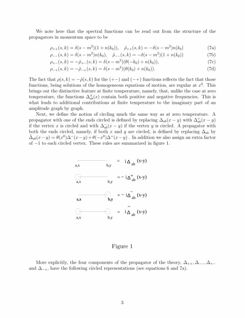
Next, we define the notion of circling much the same way as at zero temperature. Apropagator with one of the ends circled is defined by replacing ∆ab(x − y) with ∆+

ab(x − y)if the vertex x is circled and with ∆−

ab(x − y) if the vertex y is circled. A propagator withboth the ends circled, namely, if both x and y are circled, is defined by replacing ∆ab by∆ab(x−y) = θ(x0)∆−(x−y)+ θ(−x0)∆+(x−y) . In addition we also assign an extra factorof −1 to each circled vertex. These rules are summarized in figure 1.

a,x b,y

a,x b,y

a,x b,y

a,x b,y

a,x b,y

=

=

=

=

∆

∆

∆

∆

ab

ab

ab

ab

(x-y)

(x-y)

(x-y)

(x-y)

+

_

~

i

i

i

i

_ _

Figure 1

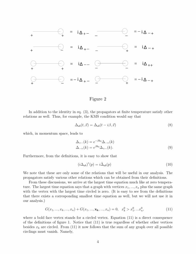
More explicitly, the four components of the propagator of the theory, ∆++, ∆−−, ∆+−

and ∆−+, have the following circled representations (see equations 6 and 7a).

3

= i ∆

∆i=

= ∆i

∆i=

i ∆

∆i=

= i∆

i= ∆

=

+

+

_

+ _

+ +

+_

+ _

++

_ _

+_ _

__

+

+

+

_

_

_

_

_

__

+

+

+

_

_

Figure 2

In addition to the identity in eq. (3), the propagators at finite temperature satisfy otherrelations as well. Thus, for example, the KMS condition would say that

∆ab(t, ~x) = ∆ab(t − iβ, ~x) (8)

which, in momentum space, leads to

∆+−(k) = e−βk0∆−+(k)

∆−+(k) = eβk0∆+−(k). (9)

Furthermore, from the definitions, it is easy to show that

(i∆ab)∗(p) = i∆ab(p) (10)

We note that these are only some of the relations that will be useful in our analysis. Thepropagators satisfy various other relations which can be obtained from their definitions.

From these discussions, we arrive at the largest time equation much like at zero tempera-ture. The largest time equation says that a graph with vertices x1, ..., xn plus the same graphwith the vertex with the largest time circled is zero. (It is easy to see from the definitionsthat there exists a corresponding smallest time equation as well, but we will not use it inour analysis.)

G(x1, ..., xk, ..., xn) + G(x1, ...,xk, ..., xn) = 0, x0k > x0

1, ...x0n, (11)

where a bold face vertex stands for a circled vertex. Equation (11) is a direct consequenceof the definitions of figure 1. Notice that (11) is true regardless of whether other verticesbesides xk are circled. From (11) it now follows that the sum of any graph over all possiblecirclings must vanish. Namely,

4

G(x1, ..., xk, ..., xn) + G(x1, ...,xk, ...,xn) +∑

circlings

G(x1, ..., xk, ..., xn) = 0, (12)

where the sum, in the last term, is over all possible circlings excluding the diagram where allvertices are circled. To show this, we observe that the sum above can be decomposed intoa sum over pairs of diagrams with a given set of circlings and with the largest time vertexcircled or uncircled. By (11) these pairs vanish and, therefore, the sum adds up pairwise tozero. Using (10) , we now see that we can write the above relation also as

Im iG(p1, ..., pm) =1

2(iG(p1, ..., pm) + (iG(p1, ..., pm))∗) = −

1

2

∑

circlings

iG(p1, ..., pm). (13)

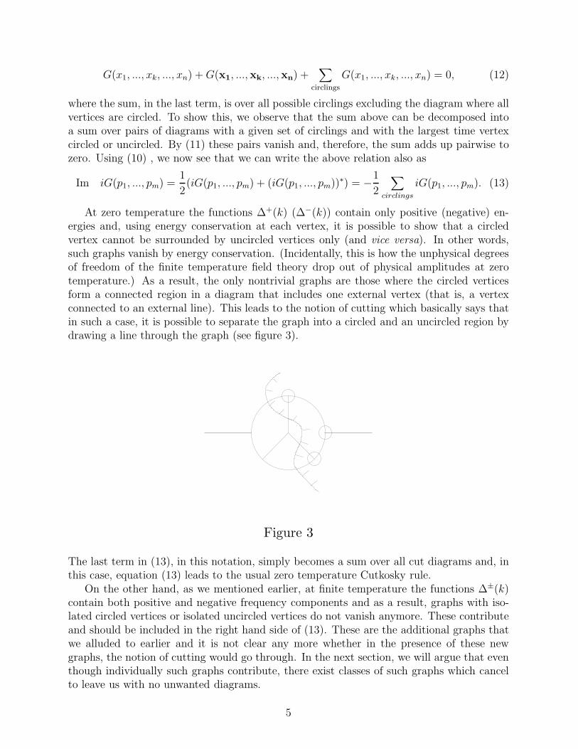
At zero temperature the functions ∆+(k) (∆−(k)) contain only positive (negative) en-ergies and, using energy conservation at each vertex, it is possible to show that a circledvertex cannot be surrounded by uncircled vertices only (and vice versa). In other words,such graphs vanish by energy conservation. (Incidentally, this is how the unphysical degreesof freedom of the finite temperature field theory drop out of physical amplitudes at zerotemperature.) As a result, the only nontrivial graphs are those where the circled verticesform a connected region in a diagram that includes one external vertex (that is, a vertexconnected to an external line). This leads to the notion of cutting which basically says thatin such a case, it is possible to separate the graph into a circled and an uncircled region bydrawing a line through the graph (see figure 3).

Figure 3

The last term in (13), in this notation, simply becomes a sum over all cut diagrams and, inthis case, equation (13) leads to the usual zero temperature Cutkosky rule.

On the other hand, as we mentioned earlier, at finite temperature the functions ∆±(k)contain both positive and negative frequency components and as a result, graphs with iso-lated circled vertices or isolated uncircled vertices do not vanish anymore. These contributeand should be included in the right hand side of (13). These are the additional graphs thatwe alluded to earlier and it is not clear any more whether in the presence of these newgraphs, the notion of cutting would go through. In the next section, we will argue that eventhough individually such graphs contribute, there exist classes of such graphs which cancelto leave us with no unwanted diagrams.

5

III. CANCELLATIONS AMONG GRAPHS

The computation of the imaginary part of any Green’s function involves a double sum atfinite temperature, namely, we have to sum over all possible circlings as in zero temperature,but in addition we must also sum over the two kinds of intermediate vertices + and − becauseof the doubled degrees of freedom. Thus, at finite temperature, for any Greens function, wehave

Im iGa...b = −1

2

∑

internal vertices=±

∑

circlings

diagram, (14)

where a...b = ± are the “thermal indices” of the external legs. As we have mentioned before,unlike the zero tempertaure case, circlings that cannot be represented by a cut diagram asin figure 2 also appear in (14). Examples of such graphs are in figure 6(i,j,k,l,m,n). All suchgraphs, however, are combinations of the same basic propagators ∆++, ∆−−, ∆+− and ∆−+

regardless of the combination of + and − vertices, circled or uncircled. We will show nowthat, after summing over the internal thermal index + and −, there are cancellations amongsuch graphs which makes unnecessary to consider unwanted kinds of circlings. The circlingsthat we are left with finally, are of the kind of those in figure 2, which can be represented bya cut diagram. This not only simplifies the evaluation of the imaginary parts by reducingthe number of graphs to be considered but also allows a physical interpretation in terms ofdeacy rates and emission/absorption of particles to/from the medium.

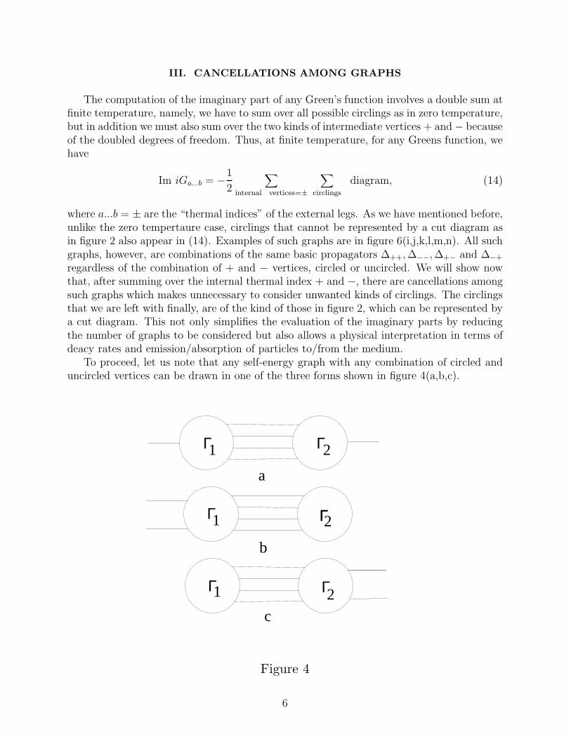
To proceed, let us note that any self-energy graph with any combination of circled anduncircled vertices can be drawn in one of the three forms shown in figure 4(a,b,c).

a

b

c

Γ

Γ

Γ

Γ

Γ

Γ

1 2

2

Γ2

1

1

Figure 4

6

Here, Γ1 is assumed to contain all the circled vertices of the graph and only the circledvertices while Γ2 contains all the uncircled vertices of the graph and only the uncircled ones.The vertices in Γ1 (or Γ2) need not all be connected to each other. The kind of diagramsthat have a non vanishing contribution to the right hand side of (13) at zero temperature arethe ones that can be drawn as in figure 4(a), with all the vertices in Γ1 connected with eachother, as well with all vertices of Γ2 connected with each other. We say that graphs of thisform can be drawn as a cut graph since a cut between Γ1 and Γ2 separates all circled verticesfrom the uncircled ones, as well as the incoming from the outgoing lines, leaving no islandof circled or uncircled vertices isolated from external lines. On the other hand, graphs suchas the ones in figure 5(b,c) cannot be represented by a cut diagram since one cannot drawa line separating a circled from uncircled vertices which will also separate the incoming andthe outgoing external lines. Graphs like figure 4(a) with Γ1 (or Γ2) disconnected can not berepresented by a cut diagram either, since a line separating Γ1 from Γ2 will also split Γ1 (Γ2)in two, leaving an cluster of circled (uncircled) vertices isolated from any external line. Wewill now show that the diagrams that can not be represented by a cut diagram, in the senseexplained above, vanish after a summation of the indices + and − of the internal vertices isperformed. This amounts to saying that the kinds of circlings that we need to consider, atfinite temperature, are precisely the ones appearing at zero temperature. To show this, weessentially need two main results.

Our first result is that any graph containing a connected cluster of circled vertices notattached to any external line must vanish. This result disposes of the graphs of the formof figure 4(c) as well as the ones of the form of figure 5(a) if Γ1 does not form a connectedset of vertices. We can see that by taking this connected cluster of circled vertices isolatedfrom external lines to be Γ1 in graphs like figure 4(c), or the component of Γ1 disconnectedfrom the external lines in graphs like figure 4(a).

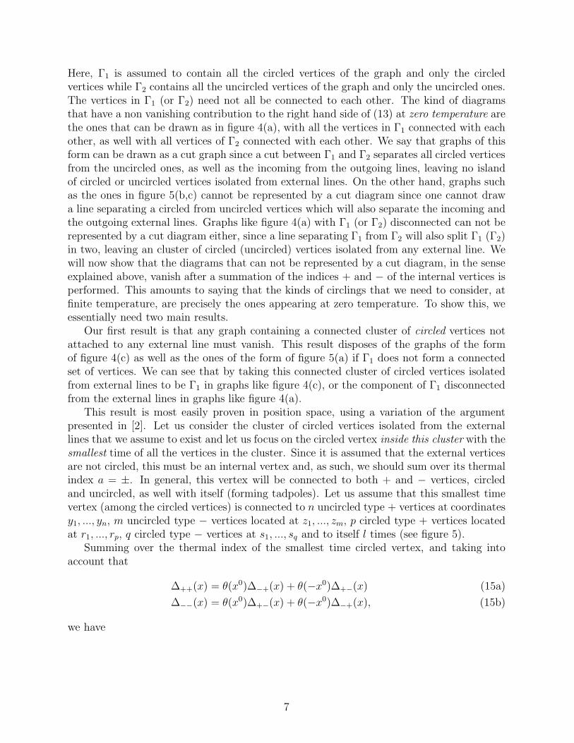
This result is most easily proven in position space, using a variation of the argumentpresented in [2]. Let us consider the cluster of circled vertices isolated from the externallines that we assume to exist and let us focus on the circled vertex inside this cluster with thesmallest time of all the vertices in the cluster. Since it is assumed that the external verticesare not circled, this must be an internal vertex and, as such, we should sum over its thermalindex a = ±. In general, this vertex will be connected to both + and − vertices, circledand uncircled, as well with itself (forming tadpoles). Let us assume that this smallest timevertex (among the circled vertices) is connected to n uncircled type + vertices at coordinatesy1, ..., yn, m uncircled type − vertices located at z1, ..., zm, p circled type + vertices locatedat r1, ..., rp, q circled type − vertices at s1, ..., sq and to itself l times (see figure 5).

Summing over the thermal index of the smallest time circled vertex, and taking intoaccount that

∆++(x) = θ(x0)∆−+(x) + θ(−x0)∆+−(x) (15a)

∆−−(x) = θ(x0)∆+−(x) + θ(−x0)∆−+(x), (15b)

we have

7

a

_

_

+

+

__

+

+

Figure 5

∑

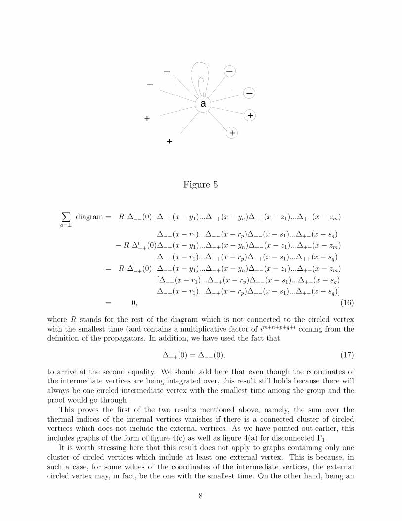
a=±

diagram = R ∆l−−(0) ∆−+(x − y1)...∆−+(x − yn)∆+−(x − z1)...∆+−(x − zm)

∆−−(x − r1)...∆−−(x − rp)∆+−(x − s1)...∆+−(x − sq)

− R ∆l++(0)∆−+(x − y1)...∆−+(x − yn)∆+−(x − z1)...∆+−(x − zm)

∆−+(x − r1)...∆−+(x − rp)∆++(x − s1)...∆++(x − sq)

= R ∆l++(0) ∆−+(x − y1)...∆−+(x − yn)∆+−(x − z1)...∆+−(x − zm)

[∆−+(x − r1)...∆−+(x − rp)∆+−(x − s1)...∆+−(x − sq)

∆−+(x − r1)...∆−+(x − rp)∆+−(x − s1)...∆+−(x − sq)]

= 0, (16)

where R stands for the rest of the diagram which is not connected to the circled vertexwith the smallest time (and contains a multiplicative factor of im+n+p+q+l coming from thedefinition of the propagators. In addition, we have used the fact that

∆++(0) = ∆−−(0), (17)

to arrive at the second equality. We should add here that even though the coordinates ofthe intermediate vertices are being integrated over, this result still holds because there willalways be one circled intermediate vertex with the smallest time among the group and theproof would go through.

This proves the first of the two results mentioned above, namely, the sum over thethermal indices of the internal vertices vanishes if there is a connected cluster of circledvertices which does not include the external vertices. As we have pointed out earlier, thisincludes graphs of the form of figure 4(c) as well as figure 4(a) for disconnected Γ1.

It is worth stressing here that this result does not apply to graphs containing only onecluster of circled vertices which include at least one external vertex. This is because, insuch a case, for some values of the coordinates of the intermediate vertices, the externalcircled vertex may, in fact, be the one with the smallest time. On the other hand, being an

8

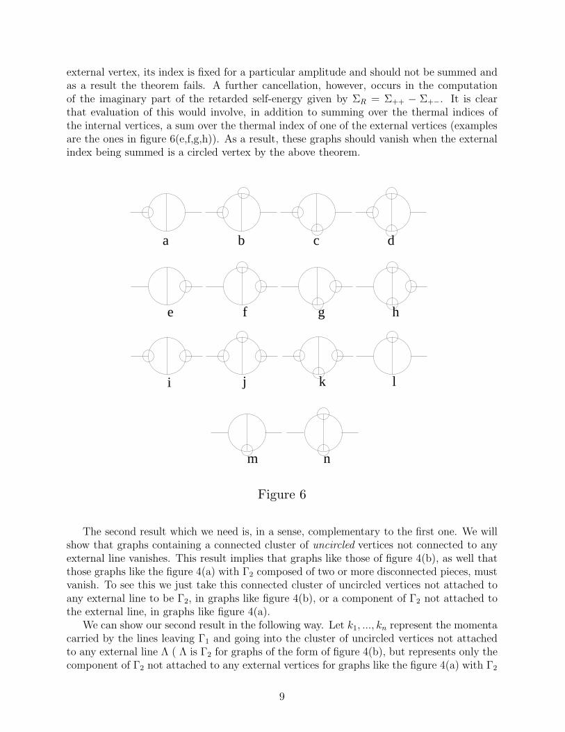
external vertex, its index is fixed for a particular amplitude and should not be summed andas a result the theorem fails. A further cancellation, however, occurs in the computationof the imaginary part of the retarded self-energy given by ΣR = Σ++ − Σ+−. It is clearthat evaluation of this would involve, in addition to summing over the thermal indices ofthe internal vertices, a sum over the thermal index of one of the external vertices (examplesare the ones in figure 6(e,f,g,h)). As a result, these graphs should vanish when the externalindex being summed is a circled vertex by the above theorem.

lkji

m n

e

a cb d

f g h

Figure 6

The second result which we need is, in a sense, complementary to the first one. We willshow that graphs containing a connected cluster of uncircled vertices not connected to anyexternal line vanishes. This result implies that graphs like those of figure 4(b), as well thatthose graphs like the figure 4(a) with Γ2 composed of two or more disconnected pieces, mustvanish. To see this we just take this connected cluster of uncircled vertices not attached toany external line to be Γ2, in graphs like figure 4(b), or a component of Γ2 not attached tothe external line, in graphs like figure 4(a).

We can show our second result in the following way. Let k1, ..., kn represent the momentacarried by the lines leaving Γ1 and going into the cluster of uncircled vertices not attachedto any external line Λ ( Λ is Γ2 for graphs of the form of figure 4(b), but represents only thecomponent of Γ2 not attached to any external vertices for graphs like the figure 4(a) with Γ2

9

disconnected). The important thing to observe here is that the propagators connecting Γ1

and Λ do not depend on the thermal indices of the vertices in Γ1, but only on the verticeson Λ. This is because these are necessarily propagators with only one end circled and asis clear from figure 2 in this case, the propagators have opposite thermal indices labelledcompletely by the uncircled vertex. Let us consider next a graph of the type of figure 4(b)(or of the type 4(a) with Γ2 disconnected) for an arbitrary fixed set of thermal indices forthe vertices that are not in Λ while we sum over the thermal indices of the Λ. For any suchconfiguration, these graphs factorize as

Σ(p) = Γ(p, k1, ..., kn)∑

α1,...,αn=±

Λα1,...,αn(k1, ..., kn)∆α1 −α1

(k1)...∆αn −αn(kn). (18)

where Λα1,...,αn(k1, ..., kn) and Γ(p, k1, ..., kn) represent the contributions coming from con-

necting the vertices in and outside of Λ respectively (as well as factors of i coming from thepropagators and vertices). The sum over each index αi of the vertices in Λα1,...,αn

(k1, ..., kn)can be performed as follows

∑

αi=±

Λ ...αi... (k1, ..., kn) ...∆αi −αi(ki) ... = Λ ...+...(k1, ..., kn) ...∆−+(ki)...

+ Λ ...−...(k1, ..., kn) ...∆+−(ki)... (19)

= ...∆+−(ki)... [Λ ...+...(k1, ..., kn)eβk0

i

+ Λ ...−...(k1, ..., kn)],

where we used the KMS condition of eq.(9)

∆−+(k) = eβk0∆+−(k), (20)

to rearrange some of the propagators. The signs associated with the +, − vertices as wellas the circlings are included in the definition of the Γ’s . After the sum over all the indicesα1, ..., αn we are left with

Σ(p) = Γ(p, k1, ..., kn)∆+−(k1)...∆+−(kn)∑

α1,...,αn=±

Λα1,...,αn(k1, ..., kn)e

β∑n

j=1

αj+1

2k0

j . (21)

Let us note here thatαj+1

2= 1 or 0 depending on whether αj = 1 or −1. The terms in

the sum above combine pairwise to produce

Λα1,...,αn(k1, ..., kn)e

β∑n

j=1

αj+1

2k0

j + Λ−α1,...,−αn(k1, ..., kn)e

β∑n

j=1

−αj+1

2k0

j

= Λ∗α1,...,αn

(k1, ..., kn) + Λ∗−α1,...,−αn

(k1, ..., kn). (22)

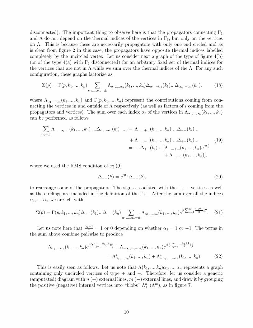
This is easily seen as follows. Let us note that Λ(k1, ..., kn)α1, ..., αn represents a graphcontaining only uncircled vertices of type + and −. Therefore, let us consider a generic(amputated) diagram with n (+) external lines, m (−) external lines, and draw it by groupingthe positive (negative) internal vertices into “blobs” Λn

+ (Λm−), as in figure 7.

10

Λ

Λ

+n

m_

Figure 7

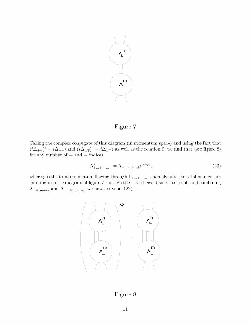
Taking the complex conjugate of this diagram (in momentum space) and using the fact that(i∆++)∗ = i∆−−) and (i∆±∓)∗ = i∆±∓) as well as the relation 9, we find that (see figure 8)for any number of + and − indices

Λ∗+...+ −...− = Λ−...− +...+e−βp0, (23)

where p is the total momentum flowing through Γ+...+ −...−, namely, it is the total momentumentering into the diagram of figure 7 through the + vertices. Using this result and combiningΛ α1,...,αn

and Λ −α1,...,−αnwe now arrive at (22).

Λ

Λ+

n

m

_

mΛ

nΛ+

_

*

=

Figure 8

11

The equation (23) can be regarded as a generalization of the KMS condition for higher pointfunctions. Returning to equation (21) we now have

Σ(p) = Γ(p, k1, ..., kn)∆+−(k1)...∆+−(kn)∑

α1,...,αn=±

Λ∗α1,...,αn

(k1, ..., kn). (24)

We can now show easily that the sum above vanishes using the largest/smallest timeargument. Let us consider a graph contributing to Λα1,...,αn

in position space and choosethe vertex with the largest time labelling its coordinate and thermal index respectively as xand a. This vertex is connected generically to n type + vertices located at y1, ..., yn and mtype − vertices located at z1, ..., zn (there are no circled vertices in Lambda). The sum overa = ± is easily seen to give

diagram = R[∆++(x − y1)...∆++(x − yn)∆+−(x − z1)...∆+−(x − zn)

−∆−+(x − y1)...∆++(x − yn)∆−−(x − z1)...∆−−(x − zn)]

= R[∆−+(x − y1)...∆−+(x − yn)∆+−(x − z1)...∆+−(x − zn)

−∆−+(x − y1)...∆−+(x − yn)∆+−(x − z1)...∆+−(x − zn)]

= 0, (25)

where R is the remaining of the diagram, independent of the vertex on x.This completes the proof of the result alluded to earlier, namely, graphs containing a

cluster of uncircled vertices not attached to any external line vanishes.With these two results, then, we see that the cutting rules for the imaginary part of any

diagram has the same form as at zero temperature. The unwanted ”extra” graphs presentat finite temperature cancel among themselves when we sum over the thermal indices of theinternal vertices. Thus, for example, it is clear now that of all the graphs in figure 6, theonly ones that will give a nontrivial contribution to the evaluation of the imaginary part ofthe the retarde self-energy are 4(a,b,c,d) ‡.

IV. PHYSICAL INTERPRETATION

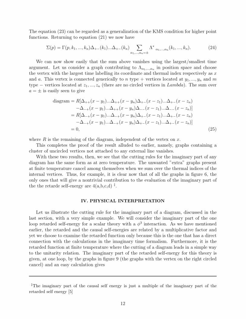
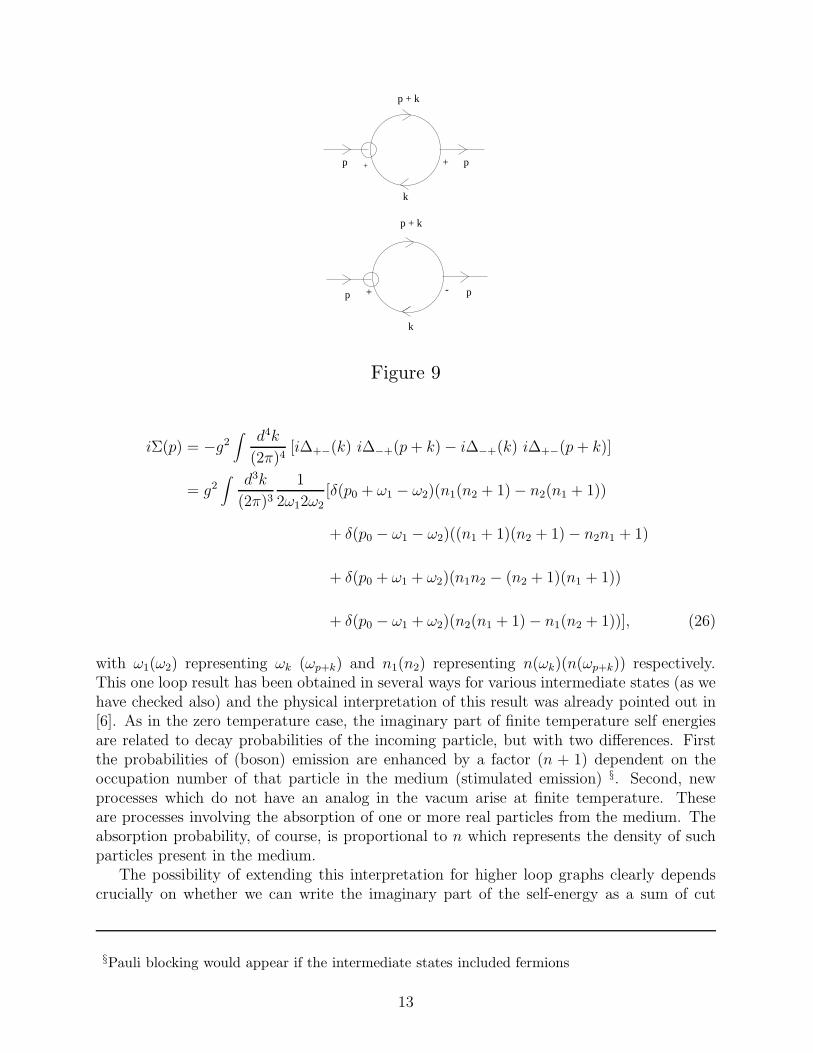
Let us illustrate the cutting rule for the imaginary part of a diagram, discussed in thelast section, with a very simple example. We will consider the imaginary part of the oneloop retarded self-energy for a scalar theory with a φ3 interaction. As we have mentionedearlier, the retarded and the causal self-energies are related by a multiplicative factor andyet we choose to examine the retarded function only because this is the one that has a directconnection with the calculations in the imaginary time formalism. Furthermore, it is theretarded function at finite temperature where the cutting of a diagram leads in a simple wayto the unitarity relation. The imaginary part of the retarded self-energy for this theory isgiven, at one loop, by the graphs in figure 9 (the graphs with the vertex on the right circledcancel) and an easy calculation gives

‡The imaginary part of the causal self energy is just a multiple of the imaginary part of the

retarded self energy [5]

12

-

k

k

p + k

p + k

p p

p p

+ +

+

Figure 9

iΣ(p) = −g2

∫ d4k

(2π)4[i∆+−(k) i∆−+(p + k) − i∆−+(k) i∆+−(p + k)]

= g2

∫ d3k

(2π)3

1

2ω12ω2

[δ(p0 + ω1 − ω2)(n1(n2 + 1) − n2(n1 + 1))

+ δ(p0 − ω1 − ω2)((n1 + 1)(n2 + 1) − n2n1 + 1)

+ δ(p0 + ω1 + ω2)(n1n2 − (n2 + 1)(n1 + 1))

+ δ(p0 − ω1 + ω2)(n2(n1 + 1) − n1(n2 + 1))], (26)

with ω1(ω2) representing ωk (ωp+k) and n1(n2) representing n(ωk)(n(ωp+k)) respectively.This one loop result has been obtained in several ways for various intermediate states (as wehave checked also) and the physical interpretation of this result was already pointed out in[6]. As in the zero temperature case, the imaginary part of finite temperature self energiesare related to decay probabilities of the incoming particle, but with two differences. Firstthe probabilities of (boson) emission are enhanced by a factor (n + 1) dependent on theoccupation number of that particle in the medium (stimulated emission) §. Second, newprocesses which do not have an analog in the vacum arise at finite temperature. Theseare processes involving the absorption of one or more real particles from the medium. Theabsorption probability, of course, is proportional to n which represents the density of suchparticles present in the medium.

The possibility of extending this interpretation for higher loop graphs clearly dependscrucially on whether we can write the imaginary part of the self-energy as a sum of cut

§Pauli blocking would appear if the intermediate states included fermions

13

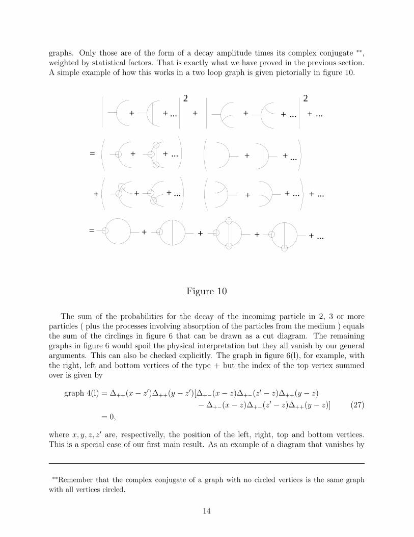
graphs. Only those are of the form of a decay amplitude times its complex conjugate ∗∗,weighted by statistical factors. That is exactly what we have proved in the previous section.A simple example of how this works in a two loop graph is given pictorially in figure 10.

+ +

22

+

++ + +

+

+

+

++ + +

+++

...

... ...+

... ......

...

...

=

=

+

+ ...

Figure 10

The sum of the probabilities for the decay of the incomimg particle in 2, 3 or moreparticles ( plus the processes involving absorption of the particles from the medium ) equalsthe sum of the circlings in figure 6 that can be drawn as a cut diagram. The remaininggraphs in figure 6 would spoil the physical interpretation but they all vanish by our generalarguments. This can also be checked explicitly. The graph in figure 6(l), for example, withthe right, left and bottom vertices of the type + but the index of the top vertex summedover is given by

graph 4(l) = ∆++(x − z′)∆++(y − z′)[∆+−(x − z)∆+−(z′ − z)∆++(y − z)

− ∆+−(x − z)∆+−(z′ − z)∆++(y − z)] (27)

= 0,

where x, y, z, z′ are, respectivelly, the position of the left, right, top and bottom vertices.This is a special case of our first main result. As an example of a diagram that vanishes by

∗∗Remember that the complex conjugate of a graph with no circled vertices is the same graph

with all vertices circled.

14

our second main result, let us take the graph in figure 4(j). Fixing, for instance, the circledvertices to be of type +, and denoting the momentum flowing from the bottom vertex tothe one on the left by k1, the momentum flowing from the bottom vertex to the one on theright by k2, and the incoming momentum by p, the sum over the bottom vertex gives

graph 4(j) = ∆−−(p + k1)∆−−(p − k2)[∆+−(k1)∆+−(k2)+−∆+−(−k1 − k2)

− ∆−+(k1)∆−+(k2)−+∆−+(−k1 − k2)] (28)

= ∆−−(p + k1)∆−−(p − k2)∆+−(k1)∆+−(k2)+−∆+−(−k1 − k2)

× (ek01+k0

2−k0

1−k0

2 − 1)

= 0.

V. CONCLUSION

We have considered the generalization of diagramatic cutting rules to the finite tempera-ture case using the real time formalism. Graphs that can not be represented by cut diagramsare shown to cancel, and those that are left have a nice interpretation in terms of decay,absorption and emission probabilities. We have concentrated on self-energy graphs but theanalysis remain virtually unchanged for graphs with more exeternal lines.

VI. ACKNOWLEDGEMENTS

One of us (A.D.) would like to thank Prof. H. Mani and the members of the Physicsgroup at the Mehta Research Institute, for their hospitality, where this work started. Thiswork was supported in part by U.S. Department of Energy grant Nos. DE-FG-02-91ER40685and DF-FC02-94ER40818.

15

REFERENCES

[1] R.E.Cutkosky, J. Math. Phys. vol. 1, 429 (1960),S.Coleman and R.E.Norton, Nuovo Cimento vol. 38, 438 (1965).

[2] G. ’t Hooft and M.Veltman, in Particle Interactions at Very High Energies , partB,D.Speiser et al. eds. (Plenum Press, NY, 1974).

[3] S. Jeon,Phys.Rev. D474586-4607 (1993), Phys.Rev. D523591-3642 (1995).[4] R.L. Kobes and G.W. Semenoff, Nucl. Phys. B260 ( 1985) 714-746, Nucl. Phys. B272 (

1986) 329-364.[5] A.A.Abrikosov, L.P.Gorkov and I.E.Dzyaloshinskii, Methods of Quantum Field Theory in

Statistical Physics, Prentice-Hall (1963).[6] H.A.Weldon, Phys. Rev. D28, 2007 (1983).

16