Cutting Plane Algorithms for Variational Inference in Graphical Models

Cutting Plane Algorithms for Variational

Inference in Graphical Models

by

David Alexander Sontag

Submitted to the Department of Electrical Engineering and ComputerScience

in partial fulfillment of the requirements for the degree of

Master of Science

at the

MASSACHUSETTS INSTITUTE OF TECHNOLOGY

May 2007

c© Massachusetts Institute of Technology 2007. All rights reserved.

Author . . . . . . . . . . . . . . . . . . . . . . . . . . . . . . . . . . . . . . . . . . . . . . . . . . . . . . . . . . . . . .Department of Electrical Engineering and Computer Science

May 25, 2007

Certified by. . . . . . . . . . . . . . . . . . . . . . . . . . . . . . . . . . . . . . . . . . . . . . . . . . . . . . . . . .Tommi S. JaakkolaAssociate Professor

Thesis Supervisor

Accepted by . . . . . . . . . . . . . . . . . . . . . . . . . . . . . . . . . . . . . . . . . . . . . . . . . . . . . . . . .Arthur C. Smith

Chairman, Department Committee on Graduate Students

2

Cutting Plane Algorithms for Variational Inference in

Graphical Models

by

David Alexander Sontag

Submitted to the Department of Electrical Engineering and Computer Scienceon May 25, 2007, in partial fulfillment of the

requirements for the degree ofMaster of Science

Abstract

In this thesis, we give a new class of outer bounds on the marginal polytope, andpropose a cutting-plane algorithm for efficiently optimizing over these constraints.When combined with a concave upper bound on the entropy, this gives a new vari-ational inference algorithm for probabilistic inference in discrete Markov RandomFields (MRFs). Valid constraints are derived for the marginal polytope through aseries of projections onto the cut polytope. Projecting onto a larger model gives anefficient separation algorithm for a large class of valid inequalities arising from eachof the original projections. As a result, we obtain tighter upper bounds on the log-partition function than possible with previous variational inference algorithms. Wealso show empirically that our approximations of the marginals are significantly moreaccurate. This algorithm can also be applied to the problem of finding the Maximuma Posteriori assignment in a MRF, which corresponds to a linear program over themarginal polytope. One of the main contributions of the thesis is to bring togethertwo seemingly different fields, polyhedral combinatorics and probabilistic inference,showing how certain results in either field can carry over to the other.

Thesis Supervisor: Tommi S. JaakkolaTitle: Associate Professor

3

4

Acknowledgments

My first two years at MIT have been a real pleasure, and I am happy to have so many

great colleagues to work with. I particularly appreciate Leslie Kaelbling’s guidance

during my first year. Working with Bonnie Berger and her group on problems in

computational biology has been very rewarding, and the problems we considered have

helped provide perspective and serve as useful examples during this more theoretical

work on approximate inference. I have also very much enjoyed being a part of the

theory group.

Over the last year I have had the great opportunity to work with and be advised

by Tommi Jaakkola, and this thesis is based on joint work with him. The dynamic

of our conversations has been tons of fun, and I am looking forward to continuing

work with Tommi over the next few years. I have also really enjoyed working with

David Karger, and am grateful to David for initially suggesting that I look at the

cutting-plane literature to tackle these inference problems. Amir Globerson has been

my partner-in-crime for approximate inference research, and has been particularly

helpful during this work, giving me the initial code for TRW and helping me debug

various problems.

Thanks also to my office and lab mates for providing a stimulating and fun envi-

ronment to work in, and to everyone who repeatedly inquired on my writing status

and endeavored to get me to stop advancing the theory and start writing already. As

always, the biggest thanks are due to my family for their constant support and pa-

tience. Finally, I thank Violeta for her love and support, for bearing with me during

my busy weeks, and for making every day a happy one.

This thesis is dedicated in memory of Sean Jalal Hanna.

5

6

Contents

1 Introduction 13

2 Background 17

2.1 Exponential Family and Graphical Models . . . . . . . . . . . . . . . 17

2.2 Exact and Approximate Inference . . . . . . . . . . . . . . . . . . . . 19

2.3 Variational Methods . . . . . . . . . . . . . . . . . . . . . . . . . . . 20

2.3.1 Naive Mean Field . . . . . . . . . . . . . . . . . . . . . . . . . 22

2.3.2 Loopy Belief Propagation . . . . . . . . . . . . . . . . . . . . 23

2.3.3 Tree-Reweighted Sum-Product . . . . . . . . . . . . . . . . . . 24

2.3.4 Log-determinant Relaxation . . . . . . . . . . . . . . . . . . . 25

2.4 Maximum a Posteriori . . . . . . . . . . . . . . . . . . . . . . . . . . 27

3 Cutting-Plane Algorithm 29

4 Cut Polytope 31

4.1 Polyhedral Results . . . . . . . . . . . . . . . . . . . . . . . . . . . . 31

4.1.1 Equivalence to Marginal Polytope . . . . . . . . . . . . . . . . 32

4.1.2 Relaxations of the Cut Polytope . . . . . . . . . . . . . . . . . 33

4.1.3 Cluster Relaxations and View from Cut Polytope . . . . . . . 34

4.2 Separation Algorithms . . . . . . . . . . . . . . . . . . . . . . . . . . 35

4.2.1 Cycle Inequalities . . . . . . . . . . . . . . . . . . . . . . . . . 35

4.2.2 Odd-wheel Inequalities . . . . . . . . . . . . . . . . . . . . . . 37

4.2.3 Other Valid Inequalities . . . . . . . . . . . . . . . . . . . . . 37

7

5 New Outer Bounds on the Marginal Polytope 39

5.1 Separation Algorithm . . . . . . . . . . . . . . . . . . . . . . . . . . . 44

5.2 Non-pairwise Markov Random Fields . . . . . . . . . . . . . . . . . . 47

5.3 Remarks on Multi-Cut Polytope . . . . . . . . . . . . . . . . . . . . . 48

6 Experiments 51

6.1 Computing Marginals . . . . . . . . . . . . . . . . . . . . . . . . . . . 51

6.2 Maximum a Posteriori . . . . . . . . . . . . . . . . . . . . . . . . . . 56

7 Conclusion 59

A Remarks on Complexity 63

8

List of Figures

5-1 Triangle MRF . . . . . . . . . . . . . . . . . . . . . . . . . . . . . . . 40

5-2 Illustration of projection from the marginal polytope of a non-binary

MRF to the cut polytope of a different graph. All valid inequalities

for the cut polytope yield valid inequalities for the marginal polytope,

though not all will be facets. These projections map vertices to vertices,

but the map will not always be onto. . . . . . . . . . . . . . . . . . . 40

5-3 Illustration of the general projection ΨGπ for one edge (i, j) ∈ E where

χi = {0, 1, 2} and χj = {0, 1, 2, 3}. The projection graph Gπ is shown

on the right, having three partitions for i and seven for j. . . . . . . . 42

5-4 Illustration of the k−projection graph for one edge (i, j) ∈ E, where

χi = {0, 1, 2}. The nodes and (some of) the edges are labeled with the

values given to them by the linear mapping, e.g. µi;0 or µij;02. . . . . 43

5-5 Illustration of the log k−projection graph for one edge (i, j) ∈ E, where

χi = {0, 1, 2, 3, 4, 5, 6, 7} and χj = {0, 1, 2, 3}. Only half of each node’s

partition is displayed; the remaining states are the other half. The q’th

partition arises from the q’th bit in the states’ binary representation. 44

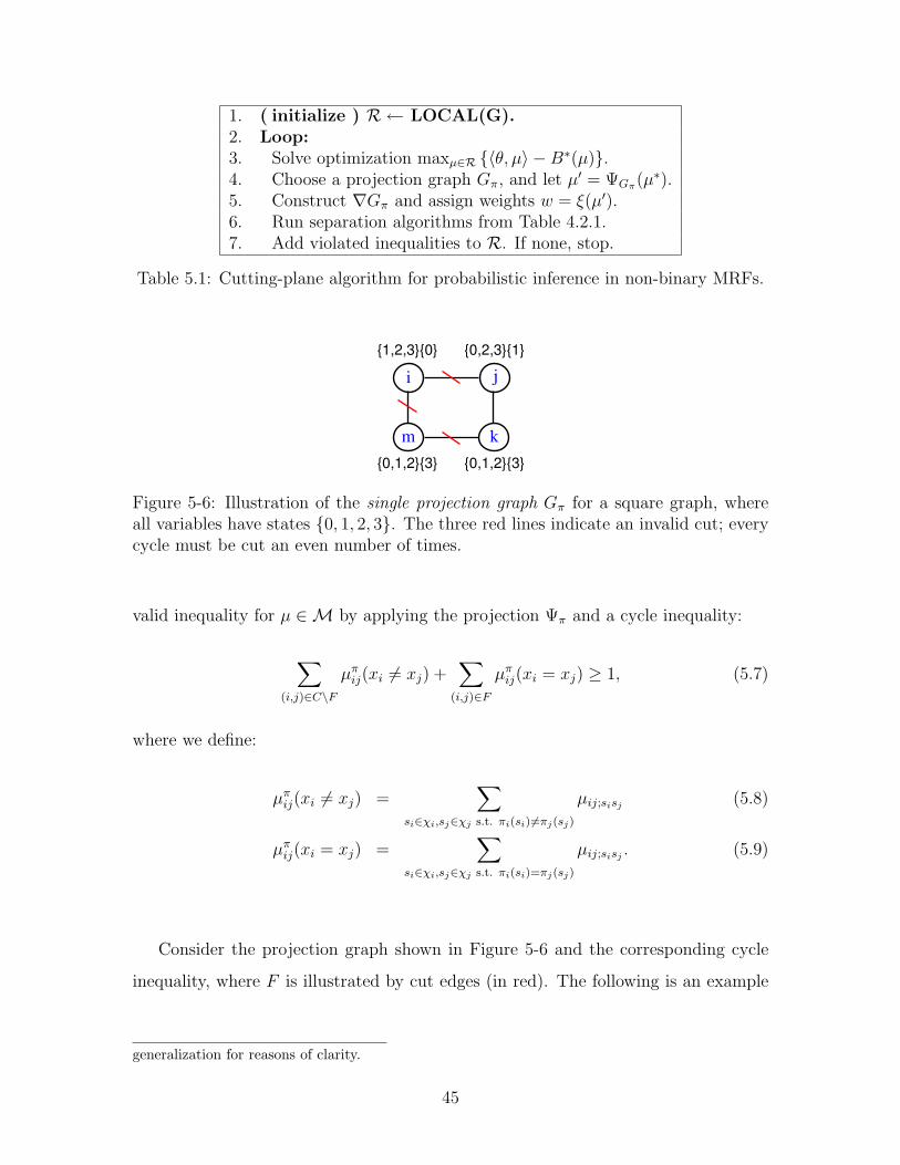
5-6 Illustration of the single projection graph Gπ for a square graph, where

all variables have states {0, 1, 2, 3}. The three red lines indicate an

invalid cut; every cycle must be cut an even number of times. . . . . 45

5-7 Example of a projection of a marginal vector from a non-pairwise MRF

to the pairwise MRF on the same variables. The original model, shown

on the left, has a potential on the variables i, j, k. . . . . . . . . . . . 47

9

6-1 Accuracy of pseudomarginals on 10 node complete graph (100 trials). 52

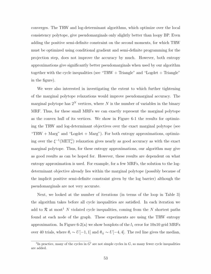
6-2 Convergence of cutting-plane algorithm with TRW entropy on 10x10

grid with θi ∈ U [−1, 1] and θij ∈ U [−4, 4] (40 trials). . . . . . . . . . 54

6-3 Convergence of cutting-plane algorithm with TRW entropy on 20 node

complete graph with θi ∈ U [−1, 1] and θij ∈ U [−4, 4] (10 trials). . . . 55

6-4 MAP on Ising grid graphs of width w × w. On the y-axis we show

the number of cycle inequalities that are added by the cutting-plane

algorithm. We found the MAP solution in all trials. . . . . . . . . . . 57

10

List of Tables

3.1 Cutting-plane algorithm for probabilistic inference in binary pairwise

MRFs. Let µ∗ be the optimum of the optimization in line 3. . . . . . 30

4.1 Summary of separation algorithms for cut polytope. . . . . . . . . . . 36

5.1 Cutting-plane algorithm for probabilistic inference in non-binary MRFs. 45

11

12

Chapter 1

Introduction

Many interesting real-world problems can be approached, from a modeling perspec-

tive, by describing a joint probability distribution over a large number of variables.

Over the last several years, graphical models have proven to be a valuable tool in

both constructing and using these probability distributions. Undirected graphical

models, also called Markov Random Fields (MRFs), are probabilistic models defined

with respect to an undirected graph. The graph’s vertices represent the variables,

and separation in the graph is equivalent to conditional independence in the distribu-

tion. The probability distribution is specified by the product of non-negative potential

functions on variables in the maximal cliques of the graph. The normalization term

is called the partition function. Given some model, we are generally interested in

two questions. The first is to find the marginal probabilities of specific subsets of

the variables, and the second is to find the most likely setting of all the variables,

called the Maximum a Posteriori (MAP) assignment. Both of these are intractable

problems and require approximate methods.

Graphical models have been successfully applied to a wide variety of fields, from

computer vision and natural language processing to computational biology. One of

the many examples of their applications in computer vision is for image segmentation.

Markov Random Fields for this problem typically have a variable for each pixel of

the image, whose value dictates which segment it belongs to. Potentials are defined

on adjacent pixels to enforce smoothness, discouraging pixels which look similar from

13

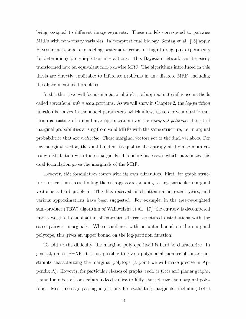
being assigned to different image segments. These models correspond to pairwise

MRFs with non-binary variables. In computational biology, Sontag et al. [16] apply

Bayesian networks to modeling systematic errors in high-throughput experiments

for determining protein-protein interactions. This Bayesian network can be easily

transformed into an equivalent non-pairwise MRF. The algorithms introduced in this

thesis are directly applicable to inference problems in any discrete MRF, including

the above-mentioned problems.

In this thesis we will focus on a particular class of approximate inference methods

called variational inference algorithms. As we will show in Chapter 2, the log-partition

function is convex in the model parameters, which allows us to derive a dual formu-

lation consisting of a non-linear optimization over the marginal polytope, the set of

marginal probabilities arising from valid MRFs with the same structure, i.e., marginal

probabilities that are realizable. These marginal vectors act as the dual variables. For

any marginal vector, the dual function is equal to the entropy of the maximum en-

tropy distribution with those marginals. The marginal vector which maximizes this

dual formulation gives the marginals of the MRF.

However, this formulation comes with its own difficulties. First, for graph struc-

tures other than trees, finding the entropy corresponding to any particular marginal

vector is a hard problem. This has received much attention in recent years, and

various approximations have been suggested. For example, in the tree-reweighted

sum-product (TRW) algorithm of Wainwright et al. [17], the entropy is decomposed

into a weighted combination of entropies of tree-structured distributions with the

same pairwise marginals. When combined with an outer bound on the marginal

polytope, this gives an upper bound on the log-partition function.

To add to the difficulty, the marginal polytope itself is hard to characterize. In

general, unless P=NP, it is not possible to give a polynomial number of linear con-

straints characterizing the marginal polytope (a point we will make precise in Ap-

pendix A). However, for particular classes of graphs, such as trees and planar graphs,

a small number of constraints indeed suffice to fully characterize the marginal poly-

tope. Most message-passing algorithms for evaluating marginals, including belief

14

propagation (sum product) and tree-reweighted sum-product, operate within the lo-

cal consistency polytope, characterized by pairwise consistent marginals. For general

graphs, the local consistency polytope is a relaxation of the marginal polytope.

We will show in Chapter 2 that finding the MAP assignment for MRFs can be

cast as an integer linear program over the marginal polytope. Thus, any relaxations

that we develop for the variational inference problem also apply to the MAP problem.

Cutting-plane algorithms are a well-known technique for solving integer linear

programs, and are often used within combinatorial optimization. These algorithms

typically begin with some relaxation of the solution space, and then find linear in-

equalities that separate the current fractional solution from all feasible integral solu-

tions, iteratively adding these constraints into the linear program. The key to such

approaches is to have an efficient separation algorithm which, given an infeasible so-

lution, can quickly find a violated constraint, generally from a very large class of valid

constraints on the set of integral solutions.

The main contribution of our work is to show how to achieve tighter outer bounds

on the marginal polytope in an efficient manner using the cutting-plane methodol-

ogy, iterating between solving a relaxed problem and adding additional constraints.

With each additional constraint, the relaxation becomes tighter. While earlier work

focused on minimizing an upper bound on the log-partition function by improving

entropy upper bounds, we minimize the upper bound on the log-partition function

by improving the outer bound on the marginal polytope.

The motivation for our approach comes from the cutting-plane literature for the

maximum cut problem. In fact, Barahona et al. [3] showed that the MAP problem

in pairwise binary MRFs is equivalent to a linear optimization over the cut polytope,

which is the convex hull of all valid graph cuts. The authors then went on to show

how tighter relaxations on the cut polytope can be achieved by using a separation

algorithm together with the cutting-plane methodology. While this work received

significant exposure in the statistical physics and operations research communities, it

went mostly unnoticed in the machine learning and statistics communities, possibly

because few interesting MRFs involve only binary variables and pairwise potentials.

15

One of our main contributions is to derive a new class of outer bounds on the

marginal polytope of non-binary and non-pairwise MRFs. The key realization is that

valid constraints can be constructed by a series of projections onto the cut polytope.

We then go on to show that projecting onto a larger graph than the original model

leads to an efficient separation algorithm for these exponentially many projections.

This result directly gives new variational inference and MAP algorithms for general

MRFs, opening the door to a completely new direction of research for the machine

learning community.

Another contribution of this thesis is to bring together two seemingly different

fields, polyhedral combinatorics and probabilistic inference. By showing how to de-

rive valid inequalities for the marginal polytope from any valid inequality on the cut

polytope, and, similarly, how to obtain tighter relaxations of the multi-cut polytope

using the marginal polytope as an extended formulation, we are creating the connec-

tion for past and future results in either field to carry over to the other. We give

various examples in this thesis of results from polyhedral combinatorics that become

particularly valuable for variational inference. Many new results in combinatorial

optimization may also turn out to be helpful for variational inference. For example,

in a recent paper [13], Krishnan et al. propose using cutting-planes for positive semi-

definite constraints, and in future work are investigating how to do so while taking

advantage of sparsity, questions which we also are very interested in. In Chapter 5 we

go the other direction, introducing new valid inequalities for the marginal polytope,

which, in turn, can be used in cutting-plane algorithms for multi-cut.

16

Chapter 2

Background

2.1 Exponential Family and Graphical Models

In this thesis, we consider inference problems in undirected graphical models, also

called Markov Random Fields or Markov networks, that are probability distributions

in the exponential family. For more details on this material, see the technical report

by Wainwright and Jordan [18].

Let x ∈ χn denote a random vector on n variables, where each variable xi takes

on the values in χi = {0, 1, . . . ,m}. The exponential family is parameterized by a set

of d potentials or sufficient statistics φ(x) = {φi} which are functions from χn to R, a

vector θ ∈ Rd, and the log-normalization (partition) function A(θ). The probability

distribution can thus be written as:

p(x; θ) = exp {〈θ, φ(x)〉 − A(θ)} (2.1)

A(θ) = log∑x∈χn

exp {〈θ, φ(x)〉} (2.2)

where 〈θ, φ(x)〉 denotes the dot product of the parameters and the sufficient statistics.

The undirected graphical model G = (V, E) has vertices V for the variables and

edges E between all vertices whose variables are together in some potential. All of our

results carry over to directed graphical models, or Bayesian networks, by the process

of moralization, in which we add undirected edges between all parents of every variable

17

and make all edges undirected. Each conditional probability distribution becomes a

potential function on its variables.

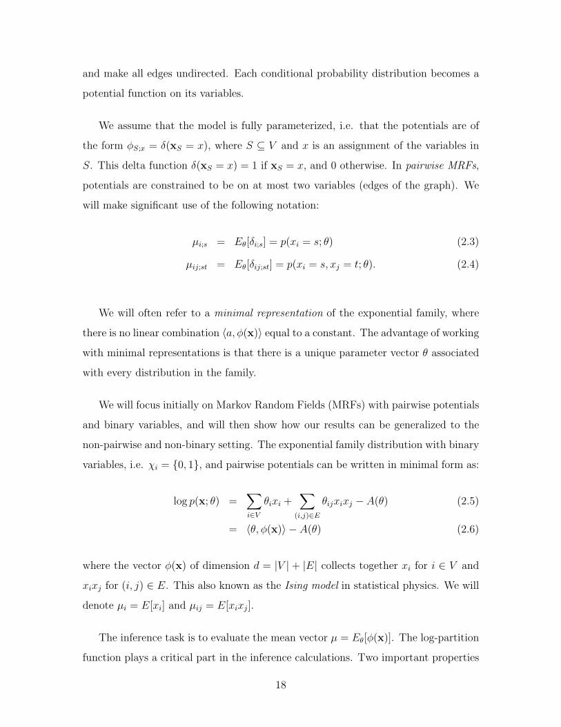
We assume that the model is fully parameterized, i.e. that the potentials are of

the form φS;x = δ(xS = x), where S ⊆ V and x is an assignment of the variables in

S. This delta function δ(xS = x) = 1 if xS = x, and 0 otherwise. In pairwise MRFs,

potentials are constrained to be on at most two variables (edges of the graph). We

will make significant use of the following notation:

µi;s = Eθ[δi;s] = p(xi = s; θ) (2.3)

µij;st = Eθ[δij;st] = p(xi = s, xj = t; θ). (2.4)

We will often refer to a minimal representation of the exponential family, where

there is no linear combination 〈a, φ(x)〉 equal to a constant. The advantage of working

with minimal representations is that there is a unique parameter vector θ associated

with every distribution in the family.

We will focus initially on Markov Random Fields (MRFs) with pairwise potentials

and binary variables, and will then show how our results can be generalized to the

non-pairwise and non-binary setting. The exponential family distribution with binary

variables, i.e. χi = {0, 1}, and pairwise potentials can be written in minimal form as:

log p(x; θ) =∑i∈V

θixi +∑

(i,j)∈E

θijxixj − A(θ) (2.5)

= 〈θ, φ(x)〉 − A(θ) (2.6)

where the vector φ(x) of dimension d = |V | + |E| collects together xi for i ∈ V and

xixj for (i, j) ∈ E. This also known as the Ising model in statistical physics. We will

denote µi = E[xi] and µij = E[xixj].

The inference task is to evaluate the mean vector µ = Eθ[φ(x)]. The log-partition

function plays a critical part in the inference calculations. Two important properties

18

of the log-partition function are:

∂A(θ)

∂θi

= Eθ[φi(x)] (2.7)

∂2A(θ)

∂θi∂θj

= Eθ[φi(x)φj(x)]− Eθ[φi(x)]Eθ[φj(x)]. (2.8)

Equation (2.8) shows that the Hessian of A(θ) is the covariance matrix of the

the probability distribution. Since covariance matrices are positive semi-definite, this

proves that A(θ) is a convex function in θ. Equation (2.7) shows that the gradient

vector of A(θ) at a point θ′ is the mean vector µ = Eθ′ [φ(x)]. These will form the

basis of the variational formulation that we will develop in Section 2.3.

2.2 Exact and Approximate Inference

Suppose we have the following tree-structured distribution:

p(x; θ) = exp

∑i∈V

∑s∈χi

θi;sφi;s(x) +∑

(i,j)∈E

∑si∈χi

∑sj∈χj

θij;sisjφij;sisj

(x)− A(θ)

(2.9)

To exactly solve for the marginals we need to compute the partition function,

given in Equation (2.2), and then do the following summation:

µ =∑x∈χn

p(x; θ)φ(x). (2.10)

In general, there will be exponentially many terms in the summations, even with

binary variables. One approach to solving this exactly, called variable elimination,

is to try to find a good ordering of the variables such that the above summation

decomposes as much as possible. Finding a good ordering for trees is easy: fix a root

node and use a depth-first traversal of the graph. The sum-product algorithm is a

dynamic programming algorithm for computing the partition function and marginals

in tree-structured MRFs. The algorithm can be applied to general MRFs by first

decomposing the graph into a junction tree, and then treating each maximal clique as

19

a variable whose values are the cross-product of the values of its constituent variables.

Such schemes will have complexity exponential in the treewidth of the graph, which

for most non-trees is quite large.

Sampling algorithms can be used to approximate the above expectations by con-

sidering only a small number of the terms in the summations [1]. One of the most

popular sampling methods is Markov chain Monte Carlo (MCMC). A Markov chain

is constructed whose stationary distribution is provably the probability distribution

of interest. We can obtain good estimates of both the partition function and the

marginals by running the chain sufficiently long to get independent samples. While

these algorithms can have nice theoretical properties, in practice it is very difficult

to prove bounds on the mixing time of these Markov chains. Even when they can be

shown, often the required running time is prohibitively large.

Another approach is to try to obtain bounds on the marginals. In the ideal

scenario, the algorithm would be able to continue improving the bounds for as long

as we run it. Bound propagation [14] is one example of an algorithm which gives

upper and lower bounds on the marginals. As we will elaborate below, variational

methods allow us to get upper and lower bounds on the partition function, which

together allow us to get bounds on the marginals.

2.3 Variational Methods

In this thesis we will focus on variational methods for approximating the log-partition

function and marginals. The convexity of A(θ) suggests an alternative definition of

the log-partition function, in terms of its Fenchel-Legendre conjugate [18]:

A(θ) = supµ∈M{〈θ, µ〉 −B(µ)} , (2.11)

where B(µ) = −H(µ) is the negative entropy of the distribution parameterized by µ

and is also convex. M is the set of realizable mean vectors µ known as the marginal

20

polytope:

M :={µ ∈ Rd | ∃p(X) s.t. µ = Ep[φ(x)]

}(2.12)

The value µ∗ ∈ M that maximizes (2.11) is precisely the desired mean vector cor-

responding to θ. One way of deriving Equation (2.11) is as follows. Let Q be any

distribution in the exponential family with sufficient statistics φ(x), let µQ = EQ[φ(x)]

be the marginal vector for Q, and let H(Q) be the entropy of Q. We have:

DKL(Q||P ) =∑x∈X

Q(x) logQ(x)

P (x)(2.13)

= −H(Q)−∑x∈X

Q(x) log P (x) (2.14)

= −H(Q)−∑x∈X

Q(x)〈θ, φ(x)〉+ A(θ) (2.15)

= −H(Q)− 〈θ, µQ〉+ A(θ) (2.16)

≥ 0. (2.17)

Re-arranging, we get

A(θ) ≥ 〈θ, µQ〉+ H(Q) (2.18)

= 〈θ, µQ〉+ H(µQ) (2.19)

where H(µQ) is the maximum entropy of all the distributions with marginals µQ.

We have an equality in the last line because the maximum entropy distribution with

those marginals is Q, since Q is in the exponential family. Since this inequality holds

for any distribution Q, and the marginal polytopeM is the set of all valid marginals

arising from some distribution, we have

A(θ) ≥ supµ∈M〈θ, µ〉+ H(µ). (2.20)

Finally, since the inequality in (2.17) is tight if and only if Q = P , the inequality

in (2.18) should be an equality, giving us (2.11). This also proves that the marginal

21

vector µ∗ which maximizes (2.20) is equal to µP .

In general bothM and the entropy H(µ) are difficult to characterize. We can try

to obtain the mean vector approximately by using an outer bound on the marginal

polytope and by bounding the entropy function. The approximate mean vectors are

called pseudomarginals. We will demonstrate later in the thesis that tighter outer

bounds onM are valuable, especially for MRFs with large couplings θij.

2.3.1 Naive Mean Field

Mean field algorithms try to find the distribution Q from a class of tractable dis-

tributions such that DKL(Q||P ) is minimized. For example, in the naive mean field

algorithm, we use the class of distributions where every node is independent of the

others (fully disconnected MRFs). As can be seen from (2.20), this yields a lower

bound on the log-partition function. This approximation corresponds to using an

inner bound on the marginal polytope, since independence implies that the pairwise

joint marginals are products of single variable marginals. The key advantage of using

this inner bound is that, for these points in the marginal polytope, the entropy can

be calculated exactly as the sum of the entropies of the individual variables. We thus

get the following naive mean field objective:

A(θ) ≥ supµ∈Mnaive

〈θ, µ〉 −∑i∈V

∑s∈χi

µi;s log µi;s (2.21)

Mnaive =

{µi;s ∈ [0, 1],

∑s∈χi

µi;s = 1, µij;st = µi;sµj;t

}(2.22)

Although the objective is not convex, we can solve for a local optimum using

gradient ascent or message-passing algorithms. The message-passing algorithms also

have an interpretation in terms of a large sample approximation of Gibbs sampling

for the model [18].

Since the approximating distribution is generally much simpler than the true dis-

tribution, and because we minimize DKL(Q||P ) and not DKL(P ||Q), mean field al-

gorithms will attempt to exactly fit some of the modes of the true distribution, while

22

ignoring the rest. For example, if we were trying to find the Gaussian distribution

which minimizes the KL-divergence to a mixture of Gaussians, we would converge

to one of the mixture components. While this does yield a lower bound on the

log-partition function, it may give a bad approximation of the marginals. An alter-

native, which we will explore extensively in this thesis, is to use an outer bound on

the marginal polytope, allowing for more interesting approximating distributions, but

paying the price of no longer having a closed form expression for the entropy.

2.3.2 Loopy Belief Propagation

One of the most popular variational inference algorithms is loopy belief propagation,

which is the sum-product algorithm applied to MRFs with cycles.

Every marginal vector must satisfy local consistency, meaning that any two pair-

wise marginals on some variable must yield, on integration, the same singleton marginal

of that variable. These constraints give us the local consistency polytope:

LOCAL(G) =

µ ≥ 0 |∑s∈χi

µi;s = 1,∑t∈χj

µij;st = µi;s

(2.23)

Since all marginals in M must satisfy (2.23), M ⊆ LOCAL(G), giving an outer

bound on the marginal polytope. For tree-structured MRFs, these constraints fully

characterize the marginal polytope, i.e. M = LOCAL(G). Furthermore, for general

graphs, both LOCAL(G) andM have the same integral vertices [18, 11].

In general it is difficult to give H(µ) exactly, because there may be many different

distributions that have the same marginal vector, each distribution having a different

entropy. In addition, for µ ∈ LOCAL(G)\M it is not clear how to define H(µ).

However, for trees, the entropy decomposes simply as the sum of the single node

23

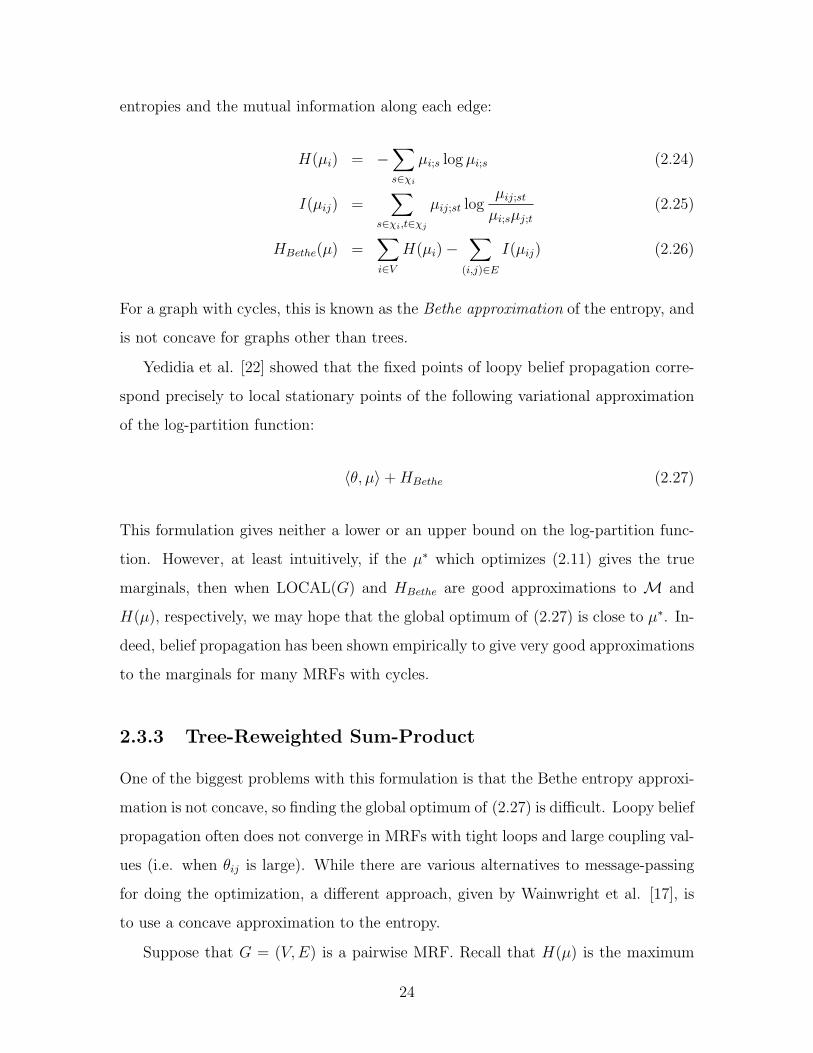
entropies and the mutual information along each edge:

H(µi) = −∑s∈χi

µi;s log µi;s (2.24)

I(µij) =∑

s∈χi,t∈χj

µij;st logµij;st

µi;sµj;t

(2.25)

HBethe(µ) =∑i∈V

H(µi)−∑

(i,j)∈E

I(µij) (2.26)

For a graph with cycles, this is known as the Bethe approximation of the entropy, and

is not concave for graphs other than trees.

Yedidia et al. [22] showed that the fixed points of loopy belief propagation corre-

spond precisely to local stationary points of the following variational approximation

of the log-partition function:

〈θ, µ〉+ HBethe (2.27)

This formulation gives neither a lower or an upper bound on the log-partition func-

tion. However, at least intuitively, if the µ∗ which optimizes (2.11) gives the true

marginals, then when LOCAL(G) and HBethe are good approximations to M and

H(µ), respectively, we may hope that the global optimum of (2.27) is close to µ∗. In-

deed, belief propagation has been shown empirically to give very good approximations

to the marginals for many MRFs with cycles.

2.3.3 Tree-Reweighted Sum-Product

One of the biggest problems with this formulation is that the Bethe entropy approxi-

mation is not concave, so finding the global optimum of (2.27) is difficult. Loopy belief

propagation often does not converge in MRFs with tight loops and large coupling val-

ues (i.e. when θij is large). While there are various alternatives to message-passing

for doing the optimization, a different approach, given by Wainwright et al. [17], is

to use a concave approximation to the entropy.

Suppose that G = (V, E) is a pairwise MRF. Recall that H(µ) is the maximum

24

entropy of all the distributions with marginals µ. Ignoring the pairwise marginals

for some of the edges can only increase the maximum entropy, since we are removing

constraints. Recall also that the entropy of a tree-structured distribution is given by

(2.26). Thus, if we were to consider µ(T ) for some T ⊆ E such that G′ = (V, T ) is a

tree, then H(µ(T )) gives a concave upper bound on H(µ).

The convex combination of the upper bounds for each spanning tree of the graph

is also an upper bound of H(µ). Minimizing this convex combination yields a tighter

bound. Let S(G) be the set of all spanning trees of the graph G. For any distribution

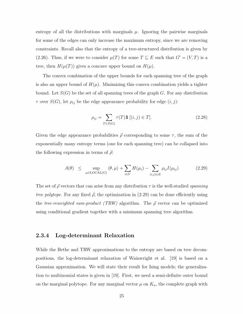
τ over S(G), let ρij be the edge appearance probability for edge (i, j):

ρij =∑

T∈S(G)

τ(T )11 [(i, j) ∈ T ]. (2.28)

Given the edge appearance probabilities ~ρ corresponding to some τ , the sum of the

exponentially many entropy terms (one for each spanning tree) can be collapsed into

the following expression in terms of ~ρ:

A(θ) ≤ supµ∈LOCAL(G)

〈θ, µ〉+∑i∈V

H(µi)−∑

(i,j)∈E

ρijI(µij) (2.29)

The set of ~ρ vectors that can arise from any distribution τ is the well-studied spanning

tree polytope. For any fixed ~ρ, the optimization in (2.29) can be done efficiently using

the tree-reweighted sum-product (TRW) algorithm. The ~ρ vector can be optimized

using conditional gradient together with a minimum spanning tree algorithm.

2.3.4 Log-determinant Relaxation

While the Bethe and TRW approximations to the entropy are based on tree decom-

positions, the log-determinant relaxation of Wainwright et al. [19] is based on a

Gaussian approximation. We will state their result for Ising models; the generaliza-

tion to multinomial states is given in [19]. First, we need a semi-definite outer bound

on the marginal polytope. For any marginal vector µ on Kn, the complete graph with

25

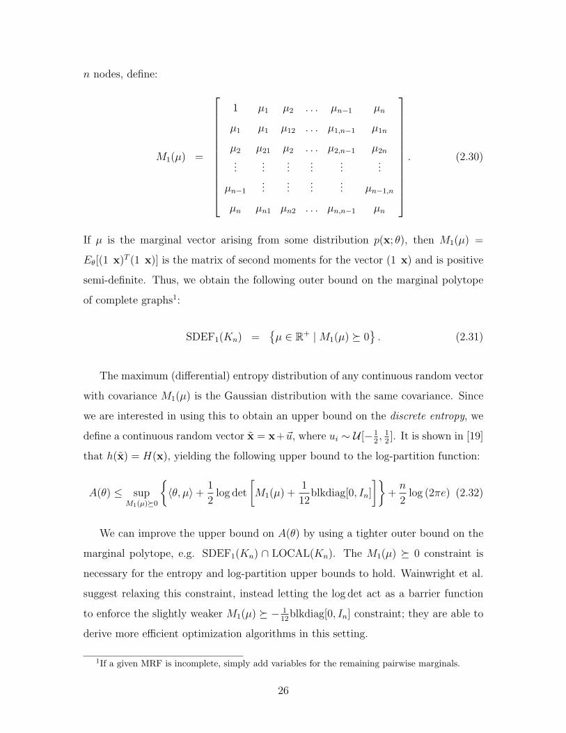
n nodes, define:

M1(µ) =

1 µ1 µ2 . . . µn−1 µn

µ1 µ1 µ12 . . . µ1,n−1 µ1n

µ2 µ21 µ2 . . . µ2,n−1 µ2n

......

......

......

µn−1...

......

... µn−1,n

µn µn1 µn2 . . . µn,n−1 µn

. (2.30)

If µ is the marginal vector arising from some distribution p(x; θ), then M1(µ) =

Eθ[(1 x)T (1 x)] is the matrix of second moments for the vector (1 x) and is positive

semi-definite. Thus, we obtain the following outer bound on the marginal polytope

of complete graphs1:

SDEF1(Kn) ={µ ∈ R+ |M1(µ) � 0

}. (2.31)

The maximum (differential) entropy distribution of any continuous random vector

with covariance M1(µ) is the Gaussian distribution with the same covariance. Since

we are interested in using this to obtain an upper bound on the discrete entropy, we

define a continuous random vector x = x+~u, where ui ∼ U [−12, 1

2]. It is shown in [19]

that h(x) = H(x), yielding the following upper bound to the log-partition function:

A(θ) ≤ supM1(µ)�0

{〈θ, µ〉+ 1

2log det

[M1(µ) +

1

12blkdiag[0, In]

]}+

n

2log (2πe) (2.32)

We can improve the upper bound on A(θ) by using a tighter outer bound on the

marginal polytope, e.g. SDEF1(Kn) ∩ LOCAL(Kn). The M1(µ) � 0 constraint is

necessary for the entropy and log-partition upper bounds to hold. Wainwright et al.

suggest relaxing this constraint, instead letting the log det act as a barrier function

to enforce the slightly weaker M1(µ) � − 112

blkdiag[0, In] constraint; they are able to

derive more efficient optimization algorithms in this setting.

1If a given MRF is incomplete, simply add variables for the remaining pairwise marginals.

26

Higher order moment matrices must also be positive semi-definite, leading to a

sequence of tighter and tighter relaxations known as the Lasserre relaxations. How-

ever, this is of little practical interest since representing higher order moments would

lead to an exponential number of variables in the relaxation. One of the conclusions

from this thesis is that an entirely different set of valid constraints, to be introduced

in Chapter 4, give more accurate pseudomarginals than the first order semi-definite

constraints, while still taking advantage of the sparsity of the graph.

2.4 Maximum a Posteriori

The MAP problem is to find the assignment x ∈ χn which maximizes P (x; θ), or

equivalently:

maxx∈χn

log P (x; θ) = maxx∈χn〈θ, φ(x)〉 − A(θ) (2.33)

= supµ∈M〈θ, µ〉 − A(θ) (2.34)

where the log-partition function A(θ) is a constant for the purpose of finding the

maximizing assignment and can be ignored. The last equality comes from the fact

that the optimal value of a linear program is attained at an extreme point or vertex,

and the extreme points of the marginal polytope are simply the delta distributions

on assignments x ∈ χn. When the MAP assignment x∗ is unique, we have that the

maximizing µ∗ = φ(x∗).

In summary, both inferring marginals and the MAP assignments correspond to

optimizing some objective over the marginal polytopeM.

27

28

Chapter 3

Cutting-Plane Algorithm

The main result in this thesis is the proposed algorithm given in Table 3. The algo-

rithm alternates between solving for an upper bound of the log-partition function (see

eqn. 2.11) and tightening the outer bound on the marginal polytope by adding valid

constraints that are violated by the pseudomarginals at the optimum µ∗. We will

discuss the actual constraints and separation algorithms in the following chapters; for

now it suffices to know that the algorithm is able to efficiently separate an exponen-

tially large class of valid constraints. In effect, we are using a significantly tighter

relaxation to the marginal polytope than LOCAL(G) without having to explicitly

represent all constraints. In Chapter 5 we show how to generalize this algorithm to

non-pairwise and non-binary MRFs.

Our results are focused on the marginal polytope, not the entropy upper bound.

Any approximation B∗(µ) of the entropy function can be used with our algorithm, as

long as we can efficiently do the optimization given in line 3 of Table 3. In particular,

we have investigated using the log-determinant and TRW entropy approximations.

They have two particularly appealing features. First, both give upper bounds on

the entropy function, and thus allow our algorithm to be used to give tighter upper

bounds on the log-partition function1. Second, the resulting objectives are convex,

allowing for efficient optimization using conditional gradient or other methods.

1In principal, our algorithm could be used with any approximation of the entropy function, e.g.the Bethe free energy approximation, which would not lead to an upper bound on the log partitionfunction, but may provide better pseudomarginals.

29

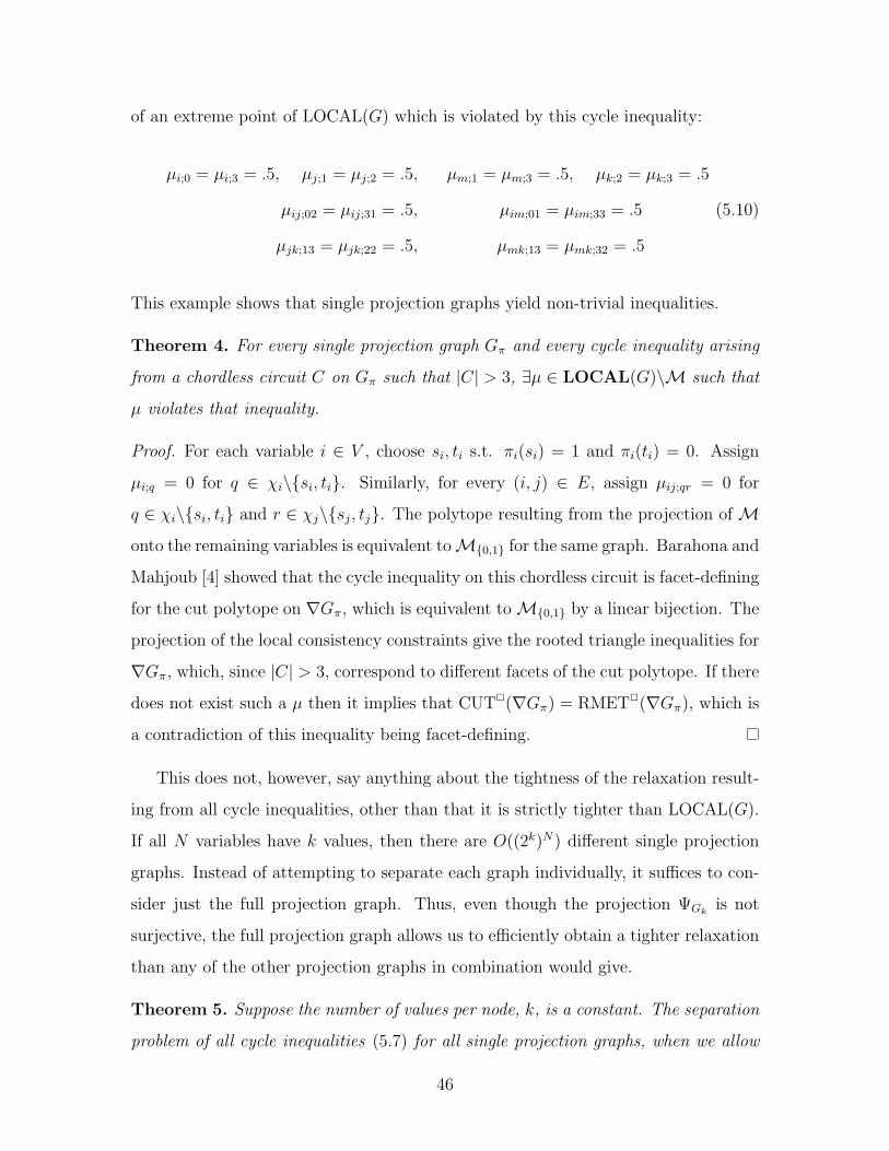
1. ( initialize ) R← LOCAL(G).2. Loop:3. Solve optimization maxµ∈R {〈θ, µ〉 −B∗(µ)}.4. Construct ∇G and assign weights w = ξ(µ∗).5. Run separation algorithms from Table 4.2.1.6. Add violated inequalities to R. If none, stop.

Table 3.1: Cutting-plane algorithm for probabilistic inference in binary pairwiseMRFs. Let µ∗ be the optimum of the optimization in line 3.

We begin with the loose outer bound on the marginal polytope given by the local

consistency constraints. It is also possible to use a tighter initial outer bound. For

example, we could include the constraint that the second moment matrix is positive

semi-definite, as described by Wainwright and Jordan [19]. The disadvantage is that it

would require explicitly representing all O(n2) µij variables2, which may be inefficient

for large yet sparse MRFs.

When the algorithm terminates, we can use the last µ∗ vector as an approximation

to the single node and pairwise marginals. The results given in Chapter 6 use this

method. An alternative would be to use the upper bounds on the partition func-

tion given by this algorithm, together with lower bounds obtained by a mean field

algorithm, in order to obtain upper and lower bounds on the marginals [12].

The algorithm for MAP is the same, but excludes the entropy function in line 3.

As a result, the optimization is simply a linear program. Since all integral vectors in

the relaxation R are extreme points of the marginal polytope, if µ∗ is integral when

the algorithm terminates, then it is the MAP assignment.

2For triangulated graphs, it suffices to constrain the maximal cliques to be PSD.

30

Chapter 4

Cut Polytope

4.1 Polyhedral Results

In this section we will show that the marginal polytope for binary pairwise MRFs1 is

equivalent to the cut polytope, which has been studied extensively within the fields

of combinatorial and polyhedral optimization [4, 2, 11]. This equivalence enables us

to translate relaxations of the cut polytope into relaxations of the marginal polytope.

Let M{0,1} denote the marginal polytope for Ising models, which we will call the

binary marginal polytope:

M{0,1} :=

µ ∈ Rd | ∃p(X) s.t.µi = Ep[Xi],

µij = Ep[XiXj]

(4.1)

Definition 1. Given a graph G = (V, E) and S ⊆ V , let δ(S) denote the vector of

RE defined for (i, j) ∈ E by,

δ(S)ij = 1 if |S ∩ {i, j}| = 1, and 0 otherwise. (4.2)

In other words, the set S gives the cut in G which separates the nodes in S from the

nodes in V \ S; δ(S)ij = 1 when i and j have different assignments. The cut polytope

1In the literature on cuts and metrics (e.g. [11]), the marginal polytope is called the correlationpolytope, and is denoted by COR2

n .

31

projected onto G is the convex hull of the above cut vectors:

CUT2(G) ={ ∑

S⊆Vn

λSδ(S) |∑S⊆Vn

λS = 1 and λS ≥ 0 for all S ⊆ Vn

}. (4.3)

The cut polytope for the complete graph on n nodes is denoted simply by CUT2n .

We should note that the cut cone is of great interest in metric embeddings, one of

the reasons being that it completely characterizes `1-embeddable metrics [11].

4.1.1 Equivalence to Marginal Polytope

Suppose that we are given a MRF defined on the graph G = (V, E). To give the

mapping between the cut polytope and the binary marginal polytope we need to

construct the suspension graph of G, denoted ∇G. Let ∇G = (V ′, E ′), where V ′ =

V ∪ {n + 1} and E ′ = E ∪ {(i, n + 1) | i ∈ V }. The suspension graph is necessary

because a cut vector δ(S) does not uniquely define an assignment to the vertices in

G – the vertices in S could be assigned either 0 or 1. Adding the extra node allows

us to remove this symmetry.

Definition 2. The linear bijection ξ from µ ∈M{0,1} to x ∈ CUT2(∇G) is given by

xi,n+1 = µi for i ∈ V and xij = µi + µj − 2µij for (i, j) ∈ E.

Using this bijection, we can reformulate the MAP problem from (2.34) as a MAX-

CUT problem2:

supµ∈M{0,1}

〈θ, µ〉 = maxx∈CUT2(∇G)

〈θ, ξ−1(x)〉. (4.4)

Furthermore, any valid inequality for the cut polytope can be transformed into

a valid inequality for the binary marginal polytope by using this mapping. In the

following sections we will describe several known relaxations of the cut polytope, all

of which directly apply to the binary marginal polytope by using the mapping.

2The edge weights may be negative, so the Goemans-Williamson approximation algorithm doesnot directly apply.

32

4.1.2 Relaxations of the Cut Polytope

It is easy to verify that every cut vector δ(S) (given in equation 4.2) must satisfy the

triangle inequalities: ∀i, j, k,

δ(S)ik + δ(S)kj − δ(S)ij ≥ 0 (4.5)

δ(S)ij + δ(S)ik + δ(S)jk ≤ 2. (4.6)

Since the cut polytope is the convex combination of cut vectors, every point x ∈ CUT2n

must also satisfy the triangle inequalities3. The semimetric polytope MET2n consists

of those points x ≥ 0 which satisfy the triangle inequalities. The projection of these

O(n3) inequalities onto an incomplete graph is non-trivial and will be addressed in

the next section. If, instead, we consider only those constraints that are defined on

the vertex n+1, we get a further relaxation, the rooted semimetric polytope RMET2n .

We can now apply the inverse mapping ξ−1 to obtain the corresponding relaxations

for the binary marginal polytope:

ξ−1(MET2n ) =

µ ∈ Rd+ |∀ i, j, k ∈ V,

µik + µkj − µk ≤ µij, and

µi + µj + µk − µij − µik − µjk ≤ 1

(4.7)

ξ−1(RMET2n ) =

µ ∈ Rd+ |∀ (i, j) ∈ E,

µij ≤ µi, µij ≤ µj

µi + µj − µij ≤ 1

(4.8)

The ξ−1(RMET2n ) polytope is equivalent to LOCAL(G) (2.23) projected onto the

variables µi;1 and µij;11. Interestingly, the triangle inequalities suffice to describe

M{0,1}, i.e. M{0,1} = ξ−1(MET2(∇G)), for a graph G if and only if G has no K4-

minor4.

3Some authors call these triplet constraints.4This result is applicable to any binary pairwise MRF. However, if we are given an Ising model

without a field, then we can construct a mapping to the cut polytope without using the suspensiongraph. By the corresponding theorem in [11], CUT(G)=MET(G) when the graph has no K5 minor,so it would be exact for planar Ising models with no field.

33

4.1.3 Cluster Relaxations and View from Cut Polytope

One approach to tightening the local consistency relaxation, used, for example, in

generalized Belief Propagation (GBP) [23], is to introduce higher-order variables to

represent the joint marginal of clusters of variables in the MRF. This improves the

approximation in two ways: 1) it results in a tighter outer bound on the marginal

polytope, and 2) these higher-order marginals can be used to get a better entropy

approximation. In particular, if we had higher-order variables for every cluster of

variables in the junction tree of a graph, it would exactly characterize the marginal

polytope.

Exactly representing the joint marginal for a cluster of n variables is equivalent

to the constraint that the projected marginal vector (onto just the variables of that

cluster) belongs to the marginal polytope on n variables. Thus, for small enough n,

an alternative to adding variables for the cluster’s joint marginal would be to use the

constraints corresponding to all of the facets of the corresponding binary marginal

polytope. Deza and Laurent [11] give complete characterizations of the cut polytope

for n ≤ 7.

Triangle inequalities, corresponding to clusters on three variables, were proposed

by various authors [19, 12] as a means of tightening the relaxation of the binary

marginal polytope. However, they were added only for those edges already present in

the MRF. The cycle inequalities that we will introduce in the next section include the

triangle inequalities as a special case. The cutting plane algorithm given in Section 3,

which separates all cycle inequalities, will result in at least as strong of a relaxation

as the triangle inequalities would give.

This perspective allows us to directly compare the relaxation to the marginal

polytope given by all triangle inequalities versus, for example, the square clusters

used for grid MRFs. The cut polytope on 5 nodes (corresponding to the four variables

in the square in addition to the suspension node) is characterized by 56 triangle

inequalities and by pentagonal inequalities [11]. Thus, by just using cycle inequalities

we are capturing the vast majority, but not all, of the facets induced by the cluster

34

variables. Furthermore, using the cluster variables alone misses out on all of the

global constraints given by the remaining cycle inequalities.

4.2 Separation Algorithms

In this section we discuss various other well-known inequalities for the cut polytope,

and show how these inequalities, though exponential in number, can be separated in

polynomial time. These separation algorithms, together with the mapping from the

cut polytope to the binary marginal polytope, form the basis of the cutting-plane

algorithm given in the previous chapter.

Each algorithm separates a different class of inequalities. All of these inequalities

arise from the study of the facets of the cut polytope. A facet is a polygon whose

corners are vertices of the polytope, i.e. a maximal (under inclusion) face. The trian-

gle inequalities, for example, are a special case of a more general class of inequalities

called the hypermetric inequalities [11] for which efficient separation algorithms are

not known. Another class, the Clique-Web inequalities, contains three special cases

for which efficient separation are known: the cycle, odd-wheel, and bicycle odd-wheel

inequalities.

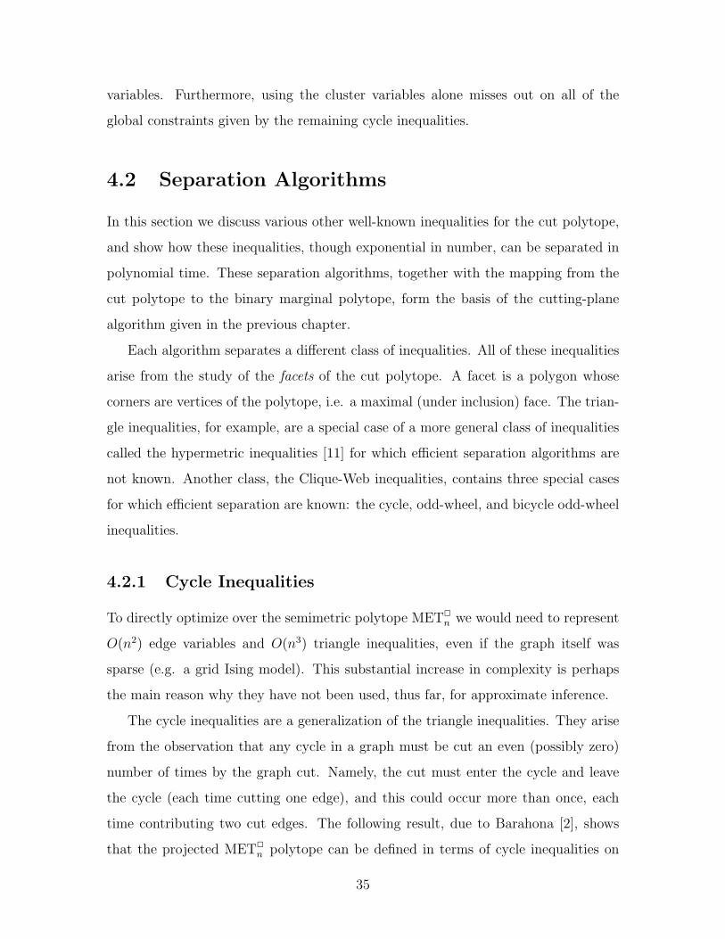
4.2.1 Cycle Inequalities

To directly optimize over the semimetric polytope MET2n we would need to represent

O(n2) edge variables and O(n3) triangle inequalities, even if the graph itself was

sparse (e.g. a grid Ising model). This substantial increase in complexity is perhaps

the main reason why they have not been used, thus far, for approximate inference.

The cycle inequalities are a generalization of the triangle inequalities. They arise

from the observation that any cycle in a graph must be cut an even (possibly zero)

number of times by the graph cut. Namely, the cut must enter the cycle and leave

the cycle (each time cutting one edge), and this could occur more than once, each

time contributing two cut edges. The following result, due to Barahona [2], shows

that the projected MET2n polytope can be defined in terms of cycle inequalities on

35

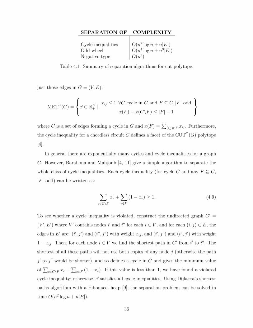
SEPARATION OF COMPLEXITY

Cycle inequalities O(n2 log n + n|E|)Odd-wheel O(n4 log n + n3|E|)Negative-type O(n3)

Table 4.1: Summary of separation algorithms for cut polytope.

just those edges in G = (V, E):

MET2(G) =

~x ∈ RE+ |

xij ≤ 1,∀C cycle in G and F ⊆ C, |F | odd

x(F )− x(C\F ) ≤ |F | − 1

where C is a set of edges forming a cycle in G and x(F ) =

∑(i,j)∈F xij. Furthermore,

the cycle inequality for a chordless circuit C defines a facet of the CUT2(G) polytope

[4].

In general there are exponentially many cycles and cycle inequalities for a graph

G. However, Barahona and Mahjoub [4, 11] give a simple algorithm to separate the

whole class of cycle inequalities. Each cycle inequality (for cycle C and any F ⊆ C,

|F | odd) can be written as:

∑e∈C\F

xe +∑e∈F

(1− xe) ≥ 1. (4.9)

To see whether a cycle inequality is violated, construct the undirected graph G′ =

(V ′, E ′) where V ′ contains nodes i′ and i′′ for each i ∈ V , and for each (i, j) ∈ E, the

edges in E ′ are: (i′, j′) and (i′′, j′′) with weight xij, and (i′, j′′) and (i′′, j′) with weight

1− xij. Then, for each node i ∈ V we find the shortest path in G′ from i′ to i′′. The

shortest of all these paths will not use both copies of any node j (otherwise the path

j′ to j′′ would be shorter), and so defines a cycle in G and gives the minimum value

of∑

e∈C\F xe +∑

e∈F (1− xe). If this value is less than 1, we have found a violated

cycle inequality; otherwise, ~x satisfies all cycle inequalities. Using Dijkstra’s shortest

paths algorithm with a Fibonacci heap [9], the separation problem can be solved in

time O(n2 log n + n|E|).

36

4.2.2 Odd-wheel Inequalities

The odd-wheel (4.10) and bicycle odd-wheel (4.11) inequalities [11] give a constraint

that any odd length cycle C must satisfy with respect to any two nodes u, v that are

not part of C:

xuv +∑e∈C

xe −∑i∈VC

(xiu + xiv) ≤ 0 (4.10)

xuv +∑e∈C

xe +∑i∈VC

(xiu + xiv) ≤ 2|VC | (4.11)

where VC refers to the vertices of cycle C. We give a sketch of the separation algorithm

for the first inequality (see [11] pgs. 481-482). The algorithm assumes that the cycle

inequalities are already satisfied. For each pair of nodes u, v, a new graph G′ is

constructed on V \{u, v} with edge weights yij = −xij + 12(xiu +xiv +xju +xjv). Since

we assumed that all the triangle inequalities were satisfied, y must be non-negative.

Then, any odd cycle C in G′ satisfies (4.10) if and only if∑

ij∈E(C) yij ≥ xuv. The

problem thus reduces to finding an odd cycle in G′ of minimum weight. This can be

solved in time O(n2 log n+n|E|) using an algorithm similar to the one we showed for

cycle inequalities.

4.2.3 Other Valid Inequalities

Another class of inequalities for the cut polytope are the negative-type inequalities

[11], which are the same as the positive semi-definite constraints on the second mo-

ment matrix [19]. While these inequalities are not facet-defining for the cut polytope,

they do provide a tighter outer bound than the local consistency polytope, and lead

to an approximation algorithm for MAX-CUT with positive edge weights. If a ma-

trix A is not positive semi-definite, a vector x can be found in O(n3) time such that

xT Ax < 0, giving us a linear constraint on A which is violated by the current solu-

tion. Thus, these inequalities can also be used in our iterative algorithm, although

the utility of doing so has not yet been determined.

If solving the relaxed problem results in a fractional solution which is outside of

37

the marginal polytope, Gomory cuts [5] provide a way of giving, in closed form, a

hyperplane which separates the fractional solution from all integral solutions. These

inequalities are applicable to MAP because any fractional solution must lie outside of

the marginal polytope. We show in Appendix A that it is NP-hard to test whether an

arbitrary point lies within the marginal polytope. Thus, Gomory cuts are not likely

to be of much use for marginals.

38

Chapter 5

New Outer Bounds on the

Marginal Polytope

In this chapter we give a new class of valid inequalities for the marginal polytope

of non-binary and non-pairwise MRFs, and show how to efficiently separate this

exponentially large set of inequalities. This contribution of our work has applicability

well beyond machine learning and statistics, as these novel inequalities can be used

within any of branch-and-cut scheme for the multi-cut problem. The key theoretical

idea will be of projections from the marginal polytope onto the cut polytope1.

The techniques of aggregation and projection as a means for obtaining valid in-

equalities are well-known in polyhedral combinatorics [11, 6, 7]. Given a linear pro-

jection Φ(x) = Ax, any valid inequality c′Φ(x) ≤ 0 for Φ(x) also gives the valid

inequality c′Ax ≤ 0 for x. Prior work used aggregation for the nodes of the graph.

Our contribution is to show how aggregation of the states of each node of the graph

can be used to obtain new inequalities for the marginal polytope.

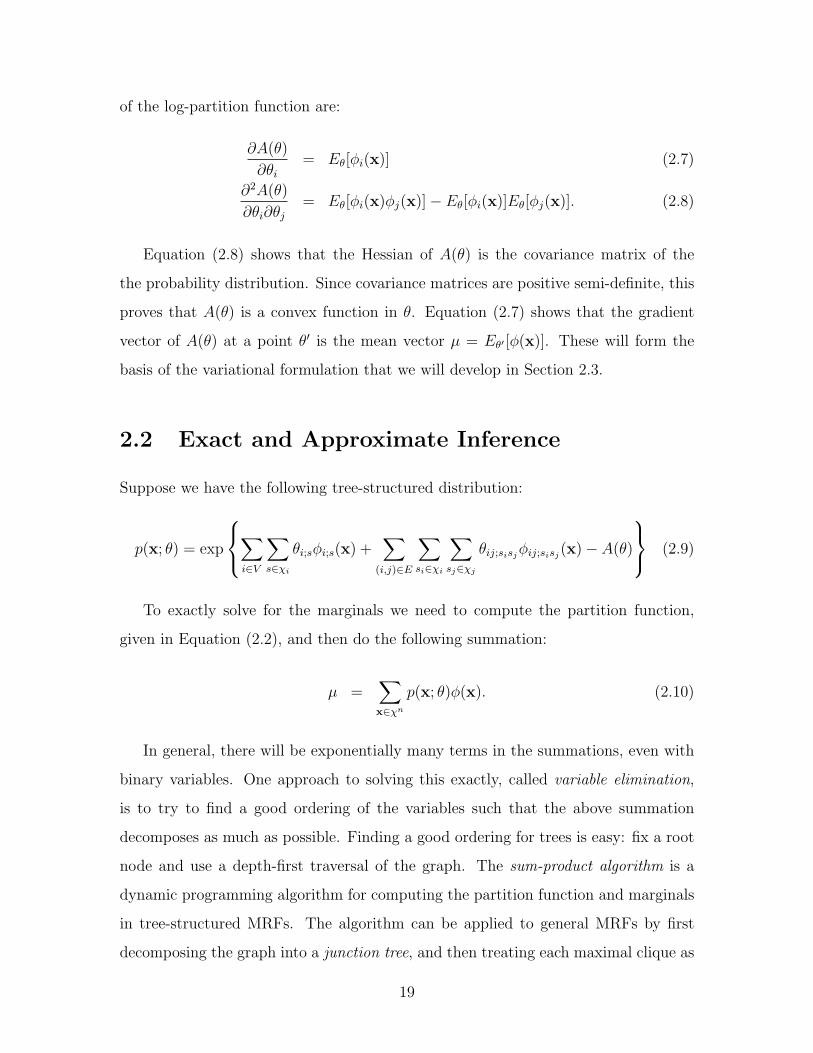
We begin by motivating why new techniques are needed for this non-binary setting.

Suppose we have the MRF in Figure 5-1 with variables taking values in χ = {0, 1, 2}

and we have a projection from µ ∈M to cut variables given by xij =∑

s,t∈χ,s 6=t µij;st.

Let x be the cut vector arising from the assignment a = 0, b = 1, c = 2. Does x

1For convenience, the projections will actually be onto the binary marginal polytope M{0,1}.Since these are equivalent via the transformation in the previous chapter, we will use their namesinterchangeably.

39

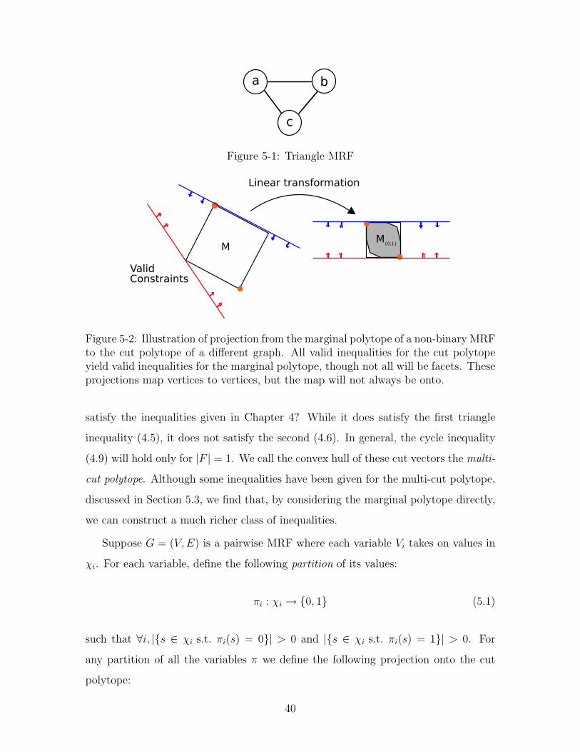
Figure 5-1: Triangle MRF

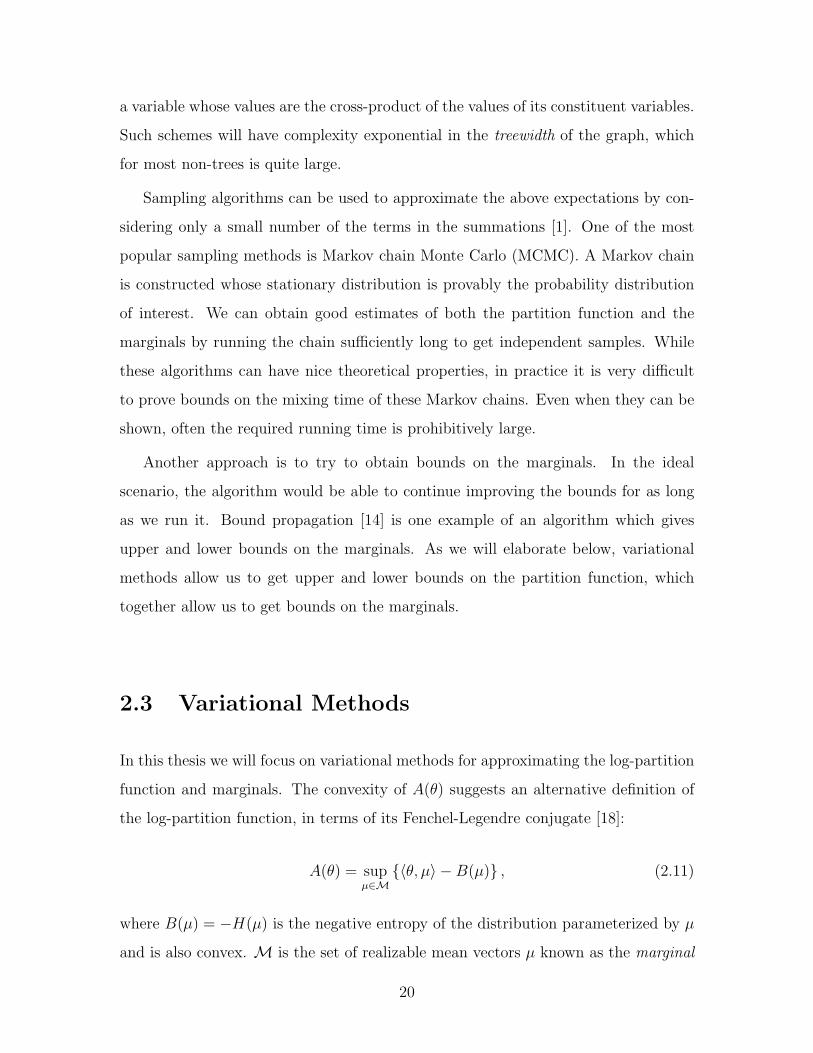
Figure 5-2: Illustration of projection from the marginal polytope of a non-binary MRFto the cut polytope of a different graph. All valid inequalities for the cut polytopeyield valid inequalities for the marginal polytope, though not all will be facets. Theseprojections map vertices to vertices, but the map will not always be onto.

satisfy the inequalities given in Chapter 4? While it does satisfy the first triangle

inequality (4.5), it does not satisfy the second (4.6). In general, the cycle inequality

(4.9) will hold only for |F | = 1. We call the convex hull of these cut vectors the multi-

cut polytope. Although some inequalities have been given for the multi-cut polytope,

discussed in Section 5.3, we find that, by considering the marginal polytope directly,

we can construct a much richer class of inequalities.

Suppose G = (V, E) is a pairwise MRF where each variable Vi takes on values in

χi. For each variable, define the following partition of its values:

πi : χi → {0, 1} (5.1)

such that ∀i, |{s ∈ χi s.t. πi(s) = 0}| > 0 and |{s ∈ χi s.t. πi(s) = 1}| > 0. For

any partition of all the variables π we define the following projection onto the cut

polytope:

40

Definition 3. The linear map Ψπ takes µ ∈ M and for i ∈ V assigns µ′i =∑s∈χi s.t. πi(s)=1 µi;s and for (i, j) ∈ E assigns µ′ij =

∑si∈χi,sj∈χj s.t. πi(si)=πj(sj)=1 µij;sisj

.

Each partition π gives a different projection, and there are O(∏

i 2|χi|) possible

partitions, or O(2Nk) if all variables have k values. To construct valid inequalities for

each projection we need to characterize the image space.

Theorem 1. The image of the projection Ψπ is M{0,1}, i.e. Ψπ : M → M{0,1}.

Furthermore, Ψπ is surjective.

Proof. Since Ψπ is a linear map, it suffices to show that, for every extreme point

µ ∈ M, Ψπ(µ) ∈ M{0,1}, and that for every extreme point µ′ ∈ M{0,1}, there exists

some µ ∈M such that Ψπ(µ) = µ′. The extreme points ofM andM{0,1} correspond

one-to-one with assignments x ∈ χn and {0, 1}n, respectively.

Given an extreme point µ ∈ M, let x′(µ)i =∑

s∈χi s.t. πi(s)=1 µi;s. Since µ is an

extreme point, µi;s = 1 for exactly one value s, which implies that x′(µ) ∈ {0, 1}n.

Then, Ψπ(µ) = E[φ(x′(µ))], showing that Ψπ(µ) ∈M{0,1}.

Given an extreme point µ′ ∈ M{0,1}, let x′(µ′) be its corresponding assignment.

For each variable i, choose some s ∈ χi such that x′(µ′)i = πi(s), and assign xi(µ′) =

s. The existence of such s is guaranteed by our construction of π. Defining µ =

E[φ(x(µ′))] ∈M, we have that Ψπ(µ) = µ′.

We will now give a more general class of projections, where we map the marginal

polytope to a cut polytope of a larger graph. The projection scheme is general, and

we will propose various classes of graphs which might be good candidates to use with

it. A cutting-plane algorithm may begin by projecting onto a smaller graph, then

advancing to projecting onto larger graphs only after satisfying all inequalities given

by the smaller one.

Let πi = {π1i , π

2i , . . .} be some set of partitions of node i. Every node can have a

different number of partitions. Define the projection graph Gπ = (Vπ, Eπ) where there

41

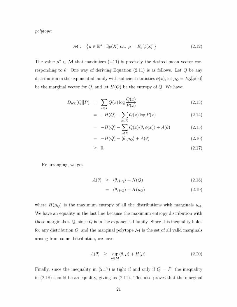
Figure 5-3: Illustration of the general projection ΨGπ for one edge (i, j) ∈ E whereχi = {0, 1, 2} and χj = {0, 1, 2, 3}. The projection graph Gπ is shown on the right,having three partitions for i and seven for j.

is a node for every partition:

Vπ =⋃i∈V

πi (5.2)

Eπ ⊆ {(πqi , π

rj ) | (i, j) ∈ E, q ≤ |πi|, r ≤ |πj|}. (5.3)

Definition 4. The linear map ΨGπ takes µ ∈ M and for each node v = πqi ∈ Vπ

assigns µ′v =∑

s∈χi s.t. πqi (s)=1 µi;s and for each edge e = (πq

i , πrj ) ∈ Eπ assigns µ′e =∑

si∈χi,sj∈χj s.t. πqi (si)=πr

j (sj)=1 µij;sisj.

This projection is a generalization of the earlier projection, where we had |πi| = 1

for all i. We call the former the single projection graph. We call the graph consisting

of all possible node partitions and all possible edges the full projection graph (see

Figure 5-3).

LetM{0,1}(Gπ) denote the binary marginal polytope of the projection graph.

Theorem 2. The image of the projection ΨGπ is M{0,1}(Gπ), i.e. Ψπ : M →

M{0,1}(Gπ).

Proof. Since ΨGπ is a linear map, it suffices to show that, for every extreme point

µ ∈M, ΨGπ(µ) ∈M{0,1}(Gπ). The extreme points ofM correspond one-to-one with

assignments x ∈ χn. Given an extreme point µ ∈M and variable v = πqi ∈ Vπ, define

x′(µ)v =∑

s∈χi s.t. πqi (s)=1 µi;s. Since µ is an extreme point, µi;s = 1 for exactly one

value s, which implies that x′(µ) ∈ {0, 1}|Vπ |. Then, ΨGπ(µ) = E[φ(x′(µ))], showing

that ΨGπ(µ) ∈M{0,1}(Gπ).

42

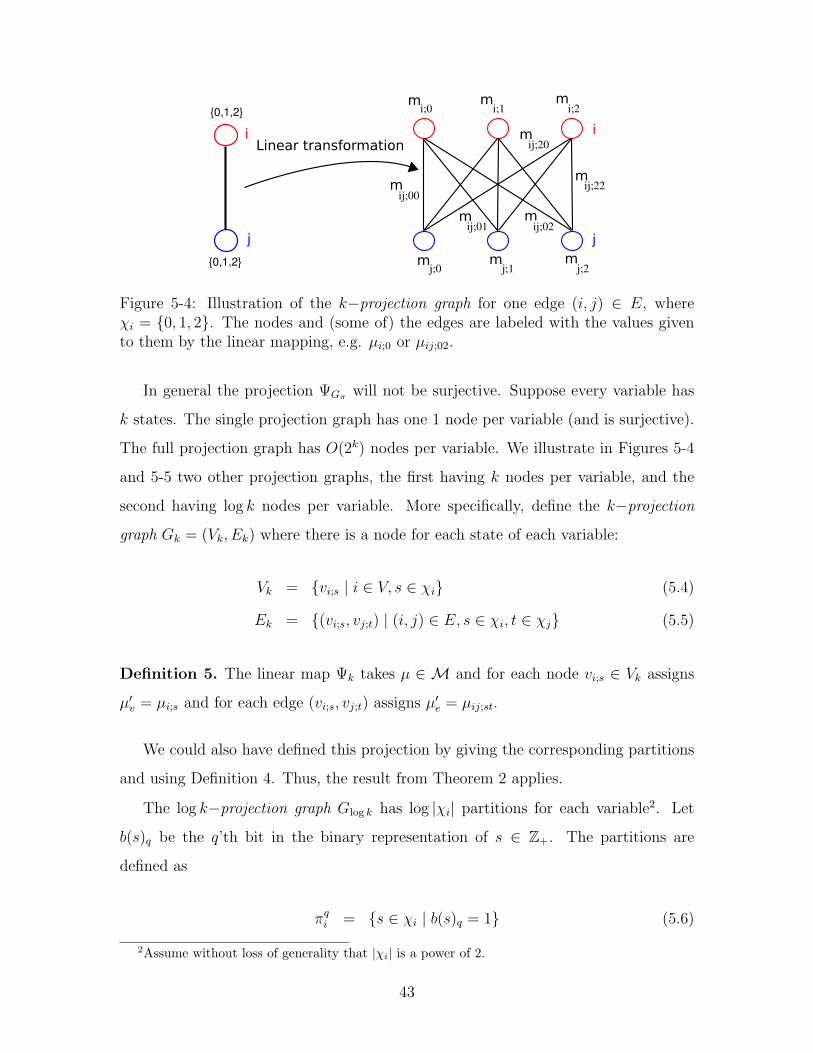
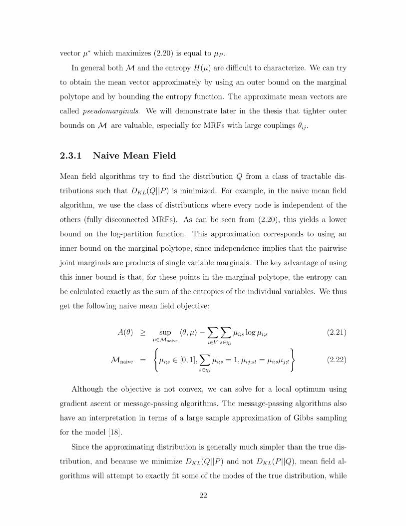
Figure 5-4: Illustration of the k−projection graph for one edge (i, j) ∈ E, whereχi = {0, 1, 2}. The nodes and (some of) the edges are labeled with the values givento them by the linear mapping, e.g. µi;0 or µij;02.

In general the projection ΨGπ will not be surjective. Suppose every variable has

k states. The single projection graph has one 1 node per variable (and is surjective).

The full projection graph has O(2k) nodes per variable. We illustrate in Figures 5-4

and 5-5 two other projection graphs, the first having k nodes per variable, and the

second having log k nodes per variable. More specifically, define the k−projection

graph Gk = (Vk, Ek) where there is a node for each state of each variable:

Vk = {vi;s | i ∈ V, s ∈ χi} (5.4)

Ek = {(vi;s, vj;t) | (i, j) ∈ E, s ∈ χi, t ∈ χj} (5.5)

Definition 5. The linear map Ψk takes µ ∈ M and for each node vi;s ∈ Vk assigns

µ′v = µi;s and for each edge (vi;s, vj;t) assigns µ′e = µij;st.

We could also have defined this projection by giving the corresponding partitions

and using Definition 4. Thus, the result from Theorem 2 applies.

The log k−projection graph Glog k has log |χi| partitions for each variable2. Let

b(s)q be the q’th bit in the binary representation of s ∈ Z+. The partitions are

defined as

πqi = {s ∈ χi | b(s)q = 1} (5.6)

2Assume without loss of generality that |χi| is a power of 2.

43

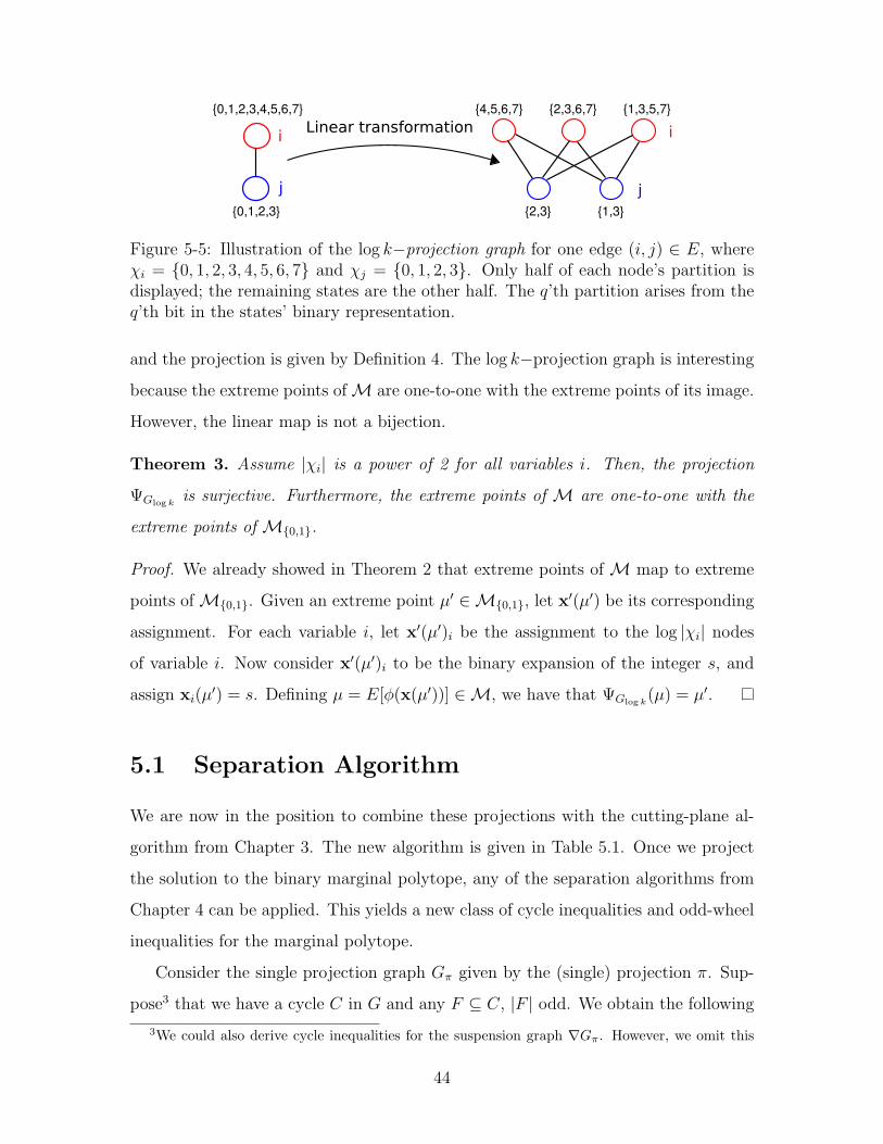
Figure 5-5: Illustration of the log k−projection graph for one edge (i, j) ∈ E, whereχi = {0, 1, 2, 3, 4, 5, 6, 7} and χj = {0, 1, 2, 3}. Only half of each node’s partition isdisplayed; the remaining states are the other half. The q’th partition arises from theq’th bit in the states’ binary representation.

and the projection is given by Definition 4. The log k−projection graph is interesting

because the extreme points ofM are one-to-one with the extreme points of its image.

However, the linear map is not a bijection.

Theorem 3. Assume |χi| is a power of 2 for all variables i. Then, the projection

ΨGlog kis surjective. Furthermore, the extreme points of M are one-to-one with the

extreme points of M{0,1}.

Proof. We already showed in Theorem 2 that extreme points of M map to extreme

points ofM{0,1}. Given an extreme point µ′ ∈M{0,1}, let x′(µ′) be its corresponding

assignment. For each variable i, let x′(µ′)i be the assignment to the log |χi| nodes

of variable i. Now consider x′(µ′)i to be the binary expansion of the integer s, and

assign xi(µ′) = s. Defining µ = E[φ(x(µ′))] ∈M, we have that ΨGlog k

(µ) = µ′.

5.1 Separation Algorithm

We are now in the position to combine these projections with the cutting-plane al-

gorithm from Chapter 3. The new algorithm is given in Table 5.1. Once we project

the solution to the binary marginal polytope, any of the separation algorithms from

Chapter 4 can be applied. This yields a new class of cycle inequalities and odd-wheel

inequalities for the marginal polytope.

Consider the single projection graph Gπ given by the (single) projection π. Sup-

pose3 that we have a cycle C in G and any F ⊆ C, |F | odd. We obtain the following

3We could also derive cycle inequalities for the suspension graph ∇Gπ. However, we omit this

44

1. ( initialize ) R← LOCAL(G).2. Loop:3. Solve optimization maxµ∈R {〈θ, µ〉 −B∗(µ)}.4. Choose a projection graph Gπ, and let µ′ = ΨGπ(µ∗).5. Construct ∇Gπ and assign weights w = ξ(µ′).6. Run separation algorithms from Table 4.2.1.7. Add violated inequalities to R. If none, stop.

Table 5.1: Cutting-plane algorithm for probabilistic inference in non-binary MRFs.

Figure 5-6: Illustration of the single projection graph Gπ for a square graph, whereall variables have states {0, 1, 2, 3}. The three red lines indicate an invalid cut; everycycle must be cut an even number of times.

valid inequality for µ ∈M by applying the projection Ψπ and a cycle inequality:

∑(i,j)∈C\F

µπij(xi 6= xj) +

∑(i,j)∈F

µπij(xi = xj) ≥ 1, (5.7)

where we define:

µπij(xi 6= xj) =

∑si∈χi,sj∈χj s.t. πi(si) 6=πj(sj)

µij;sisj(5.8)

µπij(xi = xj) =

∑si∈χi,sj∈χj s.t. πi(si)=πj(sj)

µij;sisj. (5.9)

Consider the projection graph shown in Figure 5-6 and the corresponding cycle

inequality, where F is illustrated by cut edges (in red). The following is an example

generalization for reasons of clarity.

45

of an extreme point of LOCAL(G) which is violated by this cycle inequality:

µi;0 = µi;3 = .5, µj;1 = µj;2 = .5, µm;1 = µm;3 = .5, µk;2 = µk;3 = .5

µij;02 = µij;31 = .5, µim;01 = µim;33 = .5 (5.10)

µjk;13 = µjk;22 = .5, µmk;13 = µmk;32 = .5

This example shows that single projection graphs yield non-trivial inequalities.

Theorem 4. For every single projection graph Gπ and every cycle inequality arising

from a chordless circuit C on Gπ such that |C| > 3, ∃µ ∈ LOCAL(G)\M such that

µ violates that inequality.

Proof. For each variable i ∈ V , choose si, ti s.t. πi(si) = 1 and πi(ti) = 0. Assign

µi;q = 0 for q ∈ χi\{si, ti}. Similarly, for every (i, j) ∈ E, assign µij;qr = 0 for

q ∈ χi\{si, ti} and r ∈ χj\{sj, tj}. The polytope resulting from the projection ofM

onto the remaining variables is equivalent toM{0,1} for the same graph. Barahona and

Mahjoub [4] showed that the cycle inequality on this chordless circuit is facet-defining

for the cut polytope on ∇Gπ, which is equivalent toM{0,1} by a linear bijection. The

projection of the local consistency constraints give the rooted triangle inequalities for

∇Gπ, which, since |C| > 3, correspond to different facets of the cut polytope. If there

does not exist such a µ then it implies that CUT2(∇Gπ) = RMET2(∇Gπ), which is

a contradiction of this inequality being facet-defining.

This does not, however, say anything about the tightness of the relaxation result-

ing from all cycle inequalities, other than that it is strictly tighter than LOCAL(G).

If all N variables have k values, then there are O((2k)N) different single projection

graphs. Instead of attempting to separate each graph individually, it suffices to con-

sider just the full projection graph. Thus, even though the projection ΨGkis not

surjective, the full projection graph allows us to efficiently obtain a tighter relaxation

than any of the other projection graphs in combination would give.

Theorem 5. Suppose the number of values per node, k, is a constant. The separation

problem of all cycle inequalities (5.7) for all single projection graphs, when we allow

46

Figure 5-7: Example of a projection of a marginal vector from a non-pairwise MRFto the pairwise MRF on the same variables. The original model, shown on the left,has a potential on the variables i, j, k.

some additional valid inequalities for M, can be solved in polynomial time.

Proof. All cycles in all single projection graphs are also found in the full projection

graph. Thus, by separating all cycle inequalities for the full projection graph, which

has N2k nodes, we get a strictly tighter relaxation. We showed in Chapter 4 that

the separation problem of cycle inequalities for the binary marginal polytope can be

solved in polynomial time in the size of the graph.

5.2 Non-pairwise Markov Random Fields

The results from the previous section can be trivially applied to non-pairwise MRFs

by first projecting onto a pairwise MRF, then applying the algorithm in Table 5.1. For

example, the MRF in Figure 5-7 has a potential on the variables i, j, k, so the marginal

polytope will have the variables µijk;stw for s ∈ χi, t ∈ χj, w ∈ χk. After projection,

we will have the pairwise variables µij;st, µjk;tw, and µik;sw. We can expect that the

pairwise projection will be particularly valuable for non-pairwise MRFs where the

overlap between adjacent potentials is only a single variable.

We can generalize the results of the previous section even further by considering

clusters of nodes. Suppose we include additional variables, corresponding to the

joint probability of a cluster of variables, to the marginal polytope. Figure 5-7 is an

example where i, j, k were necessarily clustered because of appearing together in a

potential. The cluster variable for i, j, k is a discrete variable taking on the values

χi × χj × χk.

We need to add constraints enforcing that all variables in common between two

47

clusters Co and Cp have the same marginals. Let Vc = Co ∩ Cp be the variables

in common between the clusters, and let Vo = Co\Vc and Vp = Cp\Vc be the other

variables. Define χc to be all possible assignments to the variables in the set Vc. Then,

for x ∈ χc, include the constraint:

∑y∈χo

µCo;x·y =∑z∈χp

µCp;x·z. (5.11)

For pairwise clusters this is simply the usual local consistency constraints. We can

now apply the projections of the previous section, considering various partitions of

each cluster variable, to obtain a tighter relaxation of the marginal polytope.

5.3 Remarks on Multi-Cut Polytope

The cut polytope has a natural multi-cut formulation called the A-partitions problem.

Suppose that every variable has at most m states. Given a pairwise MRF G = (V, E)

on n variables, construct the suspension graph ∇G = (V ′, E ′), where V ′ = V ∪

{1, . . . ,m}4, the additional m nodes corresponding to the m possible states. For each

v ∈ V having k possible states, we add edges (v, i) ∀i = 1, . . . , k to E ′ (which also

contains all of the original edges E).

While earlier we considered cuts in the graph, now we must consider partitions

π = (V1, V2, . . . , Vm) of the variables in V , where v ∈ Vi signifies that variable v has

state i. Let E(π) ⊂ E ′ be the set of edges with endpoints in different sets of the

partition (i.e. different assignments). Analogous to our definition of cut vectors (see

Definition 1) we denote δ(π) the vector of RE′defined for (i, j) ∈ E ′ by,

δ(π)ij = 1 if (i, j) ∈ E(π), and 0 otherwise. (5.12)

The multi-cut polytope is the convex hull of the δ(π) vectors for all partitions π of the

4As in the binary case, n + m− 1 nodes are possible, using a minimal representation. However,the mapping from the multi-cut polytope to the marginal polytope becomes more complex.

48

variables.5

Chopra and Owen [8] define a relaxation of the multi-cut polytope analogous to

the local consistency polytope. Although their formulation has exponentially many

constraints (in m, the maximum number of states), they show how to separate it in

polynomial time, so we could easily integrate this into our cutting-plane algorithm.

If G is a non-binary pairwise MRF which only has potentials of the form φij = δ(xi 6=

xj), called a Potts model, then the marginal polytope is in one-to-one correspondence

with the multi-cut polytope.

This formulation gives an interesting trade-off when comparing the usual local con-

sistency relaxation to the multi-cut analogue. In the former, the number of variables

are O(m|V |+ m2|E|), while in the latter, the number of variables are O(m|V |+ |E|)

but (potentially many) constraints need to be added by the cutting-plane algorithm.

It would be interesting to see whether using the multi-cut relaxation significantly

improves the running time of the LP relaxations of the Potts models in Yanover et

al. [21], where the large number of states was a hindrance.

When given a MRF which is not a Potts model, the marginal polytope is in

general not one-to-one with the multi-cut polytope; the linear mapping from the

marginal polytope to the multi-cut polytope is not injective. The results of the

previous sections can be generalized by projecting to the multi-cut polytope instead

of the cut polytope. The linear mapping xij =∑

a 6=b µij;ab would carry over valid

inequalities for the multi-cut polytope to the marginal polytope.

Chopra and Owen [8] give a per cycle class of odd cycle inequalities (exponential

in m) for the multi-cut polytope, and show how to separate these in polynomial time

(per cycle). These cycle constraints are different from the cycle constraints that we

derived in the previous section – among other differences, these constraints are for

cycles of length at most m. The authors were not able to come up with an algorithm

to separate all of their cycle inequalities in polynomial time. One open question is

whether these cycle inequalities can be derived from our projection scheme, which

5This definition is consistent with, and slightly more general than, the definition that we gave inthe beginning of the chapter.

49

would yield an efficient separation algorithm.

Various other valid inequalities have been found for the multi-cut polytope. Deza

et al. [10] generalize the clique-web inequalities to the multi-cut setting and show how,

for the special case of odd-wheel inequalities, they can be separated in polynomial

time. Borndorfer et al. [6] derive new inequalities for the multi-cut problem by

reductions to the stable set problem. In particular, their reductions give a polynomial

time algorithm for separating 2-chorded cycle inequalities.

If our original goal were to solve the multi-cut problem, the marginal polytopeM

could be considered an extended formulation of the original LP relaxations in which

we add more variables in order to obtain tighter relaxations. However, while this

directly gives an algorithm for solving multi-cut problems, actually characterizing

the implicit constraints on the multi-cut polytope is more difficult.

50

Chapter 6

Experiments

We experimented with the algorithm shown in Table 3 for both MAP and marginals.

We used the glpkmex and YALMIP [15] optimization packages within Matlab, and

wrote the separation algorithms in Java. We made no attempt to optimize our code

and thus omit running times. All of the experiments are on binary pairwise MRFs;

we expect similar results for non-binary and non-pairwise MRFs.

6.1 Computing Marginals

In this section we show that using our algorithm to optimize over the ξ−1(MET2n )

polytope yields significantly more accurate pseudomarginals than can be obtained by

optimizing over LOCAL(G). We experiment with both the log-determinant [19] and

the TRW [17] approximations of the entropy function. Although TRW can efficiently

optimize over the spanning tree polytope, for these experiments we simply use a

weighted distribution over spanning trees, where each tree’s weight is the sum of the

absolute value of its edge weights. The edge appearance probabilities corresponding

to this distribution can be efficiently computed using the Matrix Tree Theorem [20].

We optimize the TRW objective with conditional gradient, using linear programming

at each iteration to do the projection onto R.

These trials were on pairwise MRFs with xi ∈ {−1, 1} (see eqn. 2.5) and mixed

potentials. In Figure 6-1 we show results for 10 node complete graphs with θi ∼

51

1 2 3 4 5 6 7 80

0.05

0.1

0.15

0.2

0.25

0.3

0.35

0.4

0.45

0.5

Coupling term θ, drawn from U[−θ, θ]. Field is U[−1, 1]

Ave

rage

l 1 err

or o

f psu

edom

argi

nals

Loopy BPTRWTRW + PSDTRW + TriangleTRW + MargLogdetLogdet + PSDLogdet + TriangleLogdet + Marg

Figure 6-1: Accuracy of pseudomarginals on 10 node complete graph (100 trials).

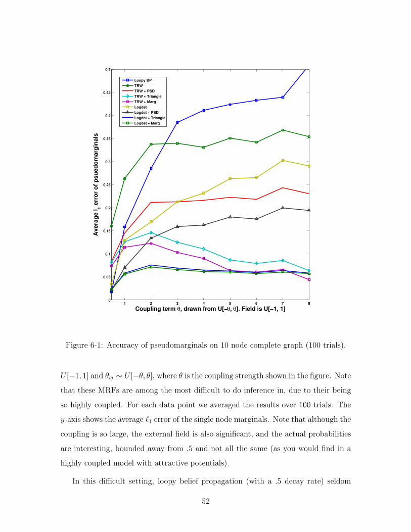
U [−1, 1] and θij ∼ U [−θ, θ], where θ is the coupling strength shown in the figure. Note

that these MRFs are among the most difficult to do inference in, due to their being

so highly coupled. For each data point we averaged the results over 100 trials. The

y-axis shows the average `1 error of the single node marginals. Note that although the

coupling is so large, the external field is also significant, and the actual probabilities

are interesting, bounded away from .5 and not all the same (as you would find in a

highly coupled model with attractive potentials).

In this difficult setting, loopy belief propagation (with a .5 decay rate) seldom

52

converges. The TRW and log-determinant algorithms, which optimize over the local

consistency polytope, give pseudomarginals only slightly better than loopy BP. Even

adding the positive semi-definite constraint on the second moments, for which TRW

must be optimized using conditional gradient and semi-definite programming for the

projection step, does not improve the accuracy by much. However, both entropy

approximations give significantly better pseudomarginals when used by our algorithm

together with the cycle inequalities (see “TRW + Triangle” and “Logdet + Triangle”

in the figure).

We were also interested in investigating the extent to which further tightening

of the marginal polytope relaxations would improve pseudomarginal accuracy. The

marginal polytope has 2N vertices, where N is the number of variables in the binary

MRF. Thus, for these small MRFs we can exactly represent the marginal polytope

as the convex hull of its vertices. We show in Figure 6-1 the results for optimiz-

ing the TRW and log-determinant objectives over the exact marginal polytope (see

“TRW + Marg” and “Logdet + Marg”). For both entropy approximations, optimiz-

ing over the ξ−1(MET2n ) relaxation gives nearly as good accuracy as with the exact

marginal polytope. Thus, for these entropy approximations, our algorithm may give

as good results as can be hoped for. However, these results are dependent on what

entropy approximation is used. For example, for a few MRFs, the solution to the log-

determinant objective already lies within the marginal polytope (possibly because of

the implicit positive semi-definite constraint given by the log barrier) although the

pseudomarginals are not very accurate.

Next, we looked at the number of iterations (in terms of the loop in Table 3)

the algorithm takes before all cycle inequalities are satisfied. In each iteration we

add to R at most1 N violated cycle inequalities, coming from the N shortest paths

found at each node of the graph. These experiments are using the TRW entropy

approximation. In Figure 6-2(a) we show boxplots of the l1 error for 10x10 grid MRFs

over 40 trials, where θi ∼ U [−1, 1] and θij ∼ U [−4, 4]. The red line gives the median,

1In practice, many of the cycles in G′ are not simple cycles in G, so many fewer cycle inequalitiesare added.

53

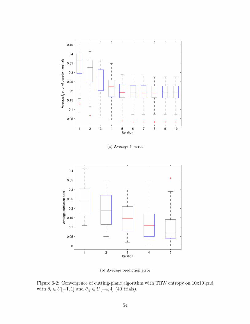
1 2 3 4 5 6 7 8 9 10

0.05

0.1

0.15

0.2

0.25

0.3

0.35

0.4

0.45

Ave

rage

l 1 err

or o

f psu

edom

argi

nals

Iteration

(a) Average `1 error

1 2 3 4 5

0

0.05

0.1

0.15

0.2

0.25

0.3

0.35

0.4

Ave

rage

pre

dict

ion

erro

r

Iteration

(b) Average prediction error

Figure 6-2: Convergence of cutting-plane algorithm with TRW entropy on 10x10 gridwith θi ∈ U [−1, 1] and θij ∈ U [−4, 4] (40 trials).

54

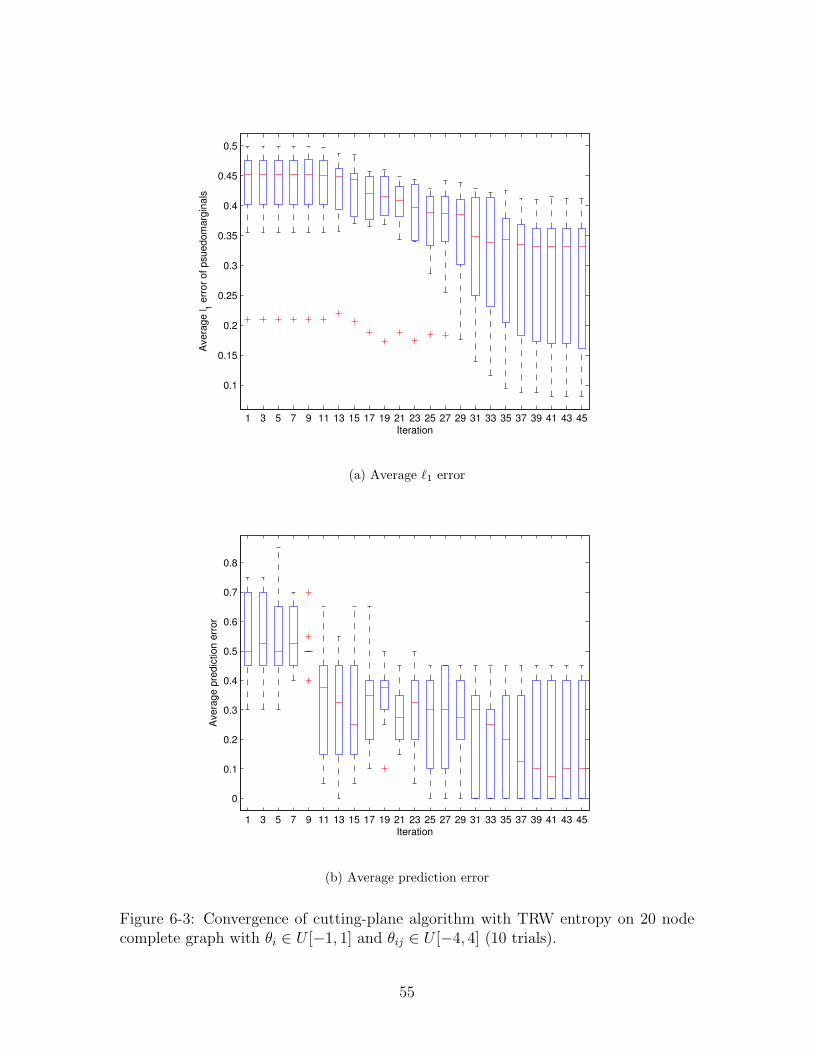
1 3 5 7 9 11 13 15 17 19 21 23 25 27 29 31 33 35 37 39 41 43 45

0.1

0.15

0.2

0.25

0.3

0.35

0.4

0.45

0.5

Ave

rage

l 1 err

or o

f psu

edom

argi

nals

Iteration

(a) Average `1 error

1 3 5 7 9 11 13 15 17 19 21 23 25 27 29 31 33 35 37 39 41 43 45

0

0.1

0.2

0.3

0.4

0.5

0.6

0.7

0.8

Ave

rage

pre

dict

ion

erro

r

Iteration

(b) Average prediction error

Figure 6-3: Convergence of cutting-plane algorithm with TRW entropy on 20 nodecomplete graph with θi ∈ U [−1, 1] and θij ∈ U [−4, 4] (10 trials).

55

and the blue boxes show the upper and lower quartiles. Iteration 1 corresponds to

TRW with only the local consistency constraints. All of the cycle inequalities were

satisfied within 10 iterations. After only 5 iterations (corresponding to solving the

TRW objective 5 times, each time using a tighter relaxation of the marginal polytope)

the median l1 error in the single node marginals dropped from over .35 to under .2.

In Figure 6-2(b) we look at whether the pseudomarginals are on the correct side of

.5 – this gives us some idea of how much improvement our algorithm would give if

we were to do classification using the marginals found by approximate inference. We

calculated the exact marginals using the Junction Tree algorithm. We observed the

same convergence results on a 30x30 grid, although we could not assess the accuracy

due to the difficulty of exact marginals calculation. From these results, we predict

that our algorithm will be both fast and accurate on larger structured models.

While these results are promising, real-world MRFs may have different structure,

so we next looked at the other extreme. In Figures 6-3(a) and 6-3(b) we give analo-

gous results for 20 node complete MRFs. In this difficult setting, the algorithm took

many more iterations before all cycle inequalities were satisfied. The total number

of cycle inequalities added was still significantly smaller than the number of triangle

inequalities on the complete graph. While the improvement in the average l1 error

is roughly monotonic as the number of iterations increase, the change in the predic-

tion accuracy is certainly not. Regardless, the eventual improvement in prediction

accuracy is striking, with the median going from .5 (as bad as a coin flip) to .1.

6.2 Maximum a Posteriori

Applying our algorithm for MAP to Ising models gives the setting already considered

by Barahona et al. [3]. We give experimental results here, both for completeness

and because we expect to observe similar results with the new outer bounds that

we introduced in Chapter 5. We should note that we are primarily interested in

the setting where we have a certificate of optimality, which our algorithm can verify

by checking that its solution is integral. Neither the max-product algorithm nor the

56

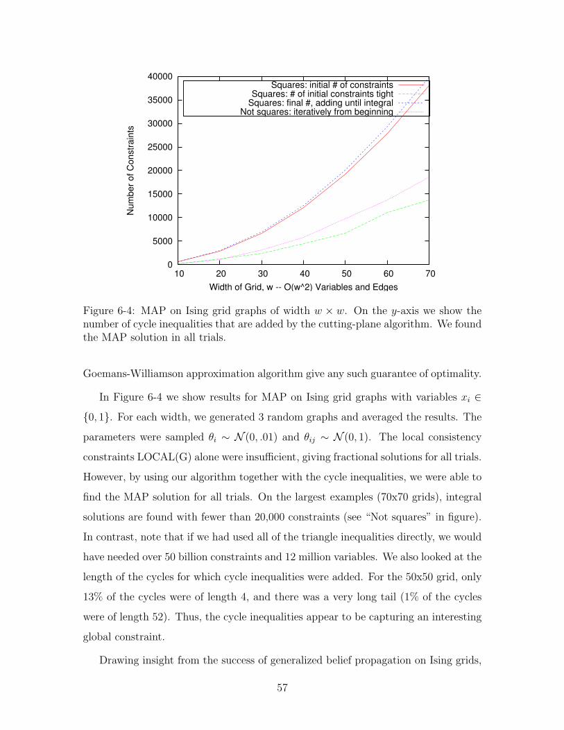
0

5000

10000

15000

20000

25000

30000

35000

40000

10 20 30 40 50 60 70

Num

ber o

f Con

stra

ints

Width of Grid, w -- O(w^2) Variables and Edges

Squares: initial # of constraintsSquares: # of initial constraints tight

Squares: final #, adding until integralNot squares: iteratively from beginning

Figure 6-4: MAP on Ising grid graphs of width w × w. On the y-axis we show thenumber of cycle inequalities that are added by the cutting-plane algorithm. We foundthe MAP solution in all trials.

Goemans-Williamson approximation algorithm give any such guarantee of optimality.

In Figure 6-4 we show results for MAP on Ising grid graphs with variables xi ∈

{0, 1}. For each width, we generated 3 random graphs and averaged the results. The

parameters were sampled θi ∼ N (0, .01) and θij ∼ N (0, 1). The local consistency

constraints LOCAL(G) alone were insufficient, giving fractional solutions for all trials.

However, by using our algorithm together with the cycle inequalities, we were able to

find the MAP solution for all trials. On the largest examples (70x70 grids), integral

solutions are found with fewer than 20,000 constraints (see “Not squares” in figure).

In contrast, note that if we had used all of the triangle inequalities directly, we would

have needed over 50 billion constraints and 12 million variables. We also looked at the

length of the cycles for which cycle inequalities were added. For the 50x50 grid, only

13% of the cycles were of length 4, and there was a very long tail (1% of the cycles

were of length 52). Thus, the cycle inequalities appear to be capturing an interesting

global constraint.

Drawing insight from the success of generalized belief propagation on Ising grids,

57

we tried initializing R to LOCAL(G) plus the O(n) length 4 cycle inequalities corre-

sponding to the squares of the grid. Interestingly, we only had to add a small number

of additional cycle inequalities before reaching the MAP solution (see “Squares: final”

in figure), resulting in much faster running times. For structured problems such as

grids, using our algorithm in this way, with a good “basis” of cycles, may be of great

practical value.

While using the cycle inequalities allowed us to find the MAP solution for all of

the grid models, we do not expect the same to hold for less structured MRFs. For

such cases, one could try using our algorithm together with branch-and-bound (these

are called branch-and-cut algorithms), in addition to trying to separate other classes

of valid inequalities for the cut polytope.

In particular, we investigated whether using the separation oracle for bicycle odd-

wheel inequalities was helpful for 30 and 40 node complete graphs, parameterized as

before. Below 30 nodes, the cycle inequalities are sufficient to find the MAP solution.

We found that, in the majority of the cases where there was a fractional solution using

just the cycle inequalities, the odd-wheel inequalities result in an integral solution,

adding between 500 and 1000 additional constraints.

58

Chapter 7

Conclusion

This thesis takes a new perspective on probabilistic inference, marrying variational in-

ference algorithms with the cutting-plane methodology of combinatorial optimization

and classical results from polyhedral combinatorics.

We show that using tighter outer bounds on the marginal polytope significantly

improves the accuracy of predicting marginal probabilities in highly coupled MRFs.

For the MRFs that we experiment with, the cutting-plane algorithm achieves these

results with only a small number of additional inequalities. One reason for why this

type of algorithm may be successful is that the marginal polytope only needs to

be well-specified near the optimum of the objective. We hope that for real-world

problems that have structure, only a small number of constraints may be necessary

to sufficiently constrain the marginal polytope at the optimum.

Our work sheds some light on the relative value of the entropy approximation

compared to the relaxation of the marginal polytope. When the MRF is weakly

coupled, both the TRW and log-determinant entropy approximations do reasonably

well using the local consistency polytope. This is not surprising: the limit of weak

coupling is a fully disconnected graph, for which both the entropy approximation

and the marginal polytope relaxation are exact. With the local consistency polytope,

both entropy approximations get steadily worse as the coupling increases. In contrast,

using the exact marginal polytope, we see a peak at θ = 2, then a steady improvement

as the coupling term grows. This occurs because the limit of strong coupling is the

59

MAP problem, for which using the exact marginal polytope will give exact results.

The interesting region is near the peak, where the entropy term is neither exact

nor outweighed by the coupling. Our algorithms seem to “solve” the part of the

problem caused by the local consistency polytope relaxation, giving nearly as good

results as the exact marginal polytope: TRW’s accuracy goes from .33 to .15, and

log-determinant’s accuracy from .17 to .076. Regardless, the fact that neither entropy

approximation can achieve accuracy below .07, even with the exact marginal polytope,

motivates further research on improving this part of the approximation.

There are various directions to proceed, further strengthening the connection to

polyhedral combinatorics. For example, many recent MRFs in vision and computa-

tional biology have matching constraints enforcing that two or more variables cannot

be assigned the same value. While these constraints are usually imposed within the

potentials, in the variational framework they correspond to taking the intersection

of the usual marginal polytope with the matching polytope for the corresponding

graph. For bipartite graphs, a linear number of constraints suffice to characterize

the matching polytope, and these can be used to give a tighter outer bound on the

marginal polytope. For general graphs, an efficient separation algorithm exists for

the matching polytope using Gomory-Hu cut trees. These constraints can be directly

used by our cutting-plane algorithm for MRFs with matching potentials.

The results in this thesis lead to several interesting open problems. The first is to

get a better understanding of the new outer bound on the marginal polytope. Which

of the inequalities obtained through projection are facet-defining for the marginal

polytope? Does considering all possible partition schemes, given by the full projection

graph, give strictly tighter relaxations than with a subset of the partition schemes such

as the k-projection graph? The second set of questions are algorithmic. Can we bound

the number of inequalities added for certain classes of MRFs? How can we project the

odd-wheel and bicycle odd-wheel inequalities to yield an efficient algorithm for sparse

graphs? Can we obtain fast separation heuristics using approximation algorithms?

Finally, can we develop new message-passing algorithms which can incorporate cycle

(and other) inequalities, to use them as an efficient inner loop in the cutting-plane

60

algorithm? Results for any of these problems would directly lead to new algorithms

for both probabilistic inference and combinatorial optimization.

61

62

Appendix A

Remarks on Complexity

A natural question that is raised in this work is whether it is possible to efficiently

test whether a point is in the marginal polytope.

Theorem 6. The following decision problem is NP-complete: given a vector µ ∈

RVn∪En+ , decide if µ ∈M.

Proof. Using the linear bijection ξ, this problem is equivalent to the decision problem

for CUT2n (the same as `1-embeddability). The latter is shown to be NP-complete in

[11].

63

64

Bibliography

[1] C. Andrieu, N. de Freitas, A. Doucet, and M. I. Jordan. An introduction toMCMC for machine learning. Machine Learning, 50:5–43, 2003.

[2] F. Barahona. On cuts and matchings in planar graphs. Mathematical Program-ming, 60:53–68, 1993.

[3] F. Barahona, M. Grotschel, M. Junger, and G. Reinelt. An application of combi-natorial optimization to statistical physics and circuit layout design. OperationsResearch, 36(3):493–513, 1988.

[4] F. Barahona and A. R. Mahjoub. On the cut polytope. Mathematical Program-ming, 36:157–173, 1986.

[5] D. Bertsimas and J. N. Tsitsiklis. Introduction to Linear Optimization. AthenaScientific, 1997.

[6] R. Borndorfer and R. Weismantel. Set packing relaxations of some integer pro-grams. Mathematical Programming, 88:425–450, 2000. ZIB Report 97-30.

[7] R. Borndorfer and R. Weismantel. Discrete relaxations of combinatorial pro-grams. Discrete Applied Mathematics, 112(1–3):11–26, 2001. ZIB Report 97-54.

[8] S. Chopra and J. Owen. Extended formulations of the A-cut problem. Mathe-matical Programming, 73:7–30, 1996.

[9] T. H. Cormen, C. E. Leiserson, R. L. Rivest, and C. Stein. Introduction toAlgorithms. MIT Press, 2nd edition, 2001.

[10] M. Deza, M. Grotschel, and M. Laurent. Clique-web facets for multicut poly-topes. Math. Oper. Res., 17(4):981–1000, 1992.

[11] M. M. Deza and M. Laurent. Geometry of Cuts and Metrics, volume 15 ofAlgorithms and Combinatorics. Springer, 1997.

[12] A. Globerson and T. Jaakkola. Approximate inference using planar graph de-composition. In Advances in Neural Information Processing Systems 20. 2007.

[13] K. Krishnan and J. E. Mitchell. A semidefinite programming based polyhedralcut and price approach for the maxcut problem. Comput. Optim. Appl., 33(1):51–71, 2006.

65

[14] M. Leisink and B. Kappen. Bound propagation. Journal of Artificial IntelligenceResearch, 19:139–154, 2003.

[15] J. Lofberg. Yalmip : A toolbox for modeling and optimization in MATLAB. InProceedings of the CACSD Conference, Taipei, Taiwan, 2004.

[16] D. Sontag, R. Singh, and B. Berger. Probabilistic modeling of systematic errorsin two-hybrid experiments. Pacific Symposium on Biocomputing, 12:445–457,2007.

[17] M. Wainwright, T. Jaakkola, and A. Willsky. A new class of upper bounds on thelog partition function. IEEE Transactions on Information Theory, 51:2313–2335,July 2005.

[18] M. Wainwright and M. I. Jordan. Graphical models, exponential families andvariational inference. Technical Report 649, UC Berkeley, Dept. of Statistics,2003.

[19] M. Wainwright and M. I. Jordan. Log-determinant relaxation for approximateinference in discrete Markov random fields. IEEE Transactions on Signal Pro-cessing, 54(6):2099–2109, June 2006.

[20] D. B. West. Introduction to Graph Theory. Prentice Hall, 2001.

[21] C. Yanover, T. Meltzer, and Y. Weiss. Linear programming relaxations and beliefpropagation – an empirical study. JMLR Special Issue on Machine Learning andLarge Scale Optimization, 7:1887–1907, September 2006.

[22] J. Yedidia, W. Freeman, and Y. Weiss. Bethe free energy, Kikuchi approxi-mations, and belief propagation algorithms. Technical Report 16, MitsubishiElectric Research Lab, 2001.

[23] J.S. Yedidia, W.T. Freeman, and Y. Weiss. Constructing free-energy approxi-mations and generalized belief propagation algorithms. IEEE Transactions onInformation Theory, 51(7):2282– 2312, July 2005.

66