Cutting Insert and Parameter Optimization for Turning Based ...

applied sciences

Article

Cutting Insert and Parameter Optimization forTurning Based on Artificial Neural Networks anda Genetic Algorithm

Bolivar Solarte-Pardo 1, Diego Hidalgo 2 and Syh-Shiuh Yeh 3,*1 Department of Mechanical and Electrical Engineering, National Taipei University of Technology,

Taipei 10608, Taiwan; [email protected] Department of Mechanical and Automation Engineering, National Taipei University of Technology,

Taipei 10608, Taiwan; [email protected] Department of Mechanical Engineering, National Taipei University of Technology, Taipei 10608, Taiwan* Correspondence: [email protected]; Tel.: +886-2-27712171

Received: 2 January 2019; Accepted: 28 January 2019; Published: 30 January 2019��

Featured Application: People and companies involved on the manufacturing industry will beable to save plenty of time on the selection of cutting inserts and parameters by implementingand using the optimization system developed in this research.

Abstract: The objective of this present study is to develop a system to optimize cutting insert selectionand cutting parameters. The proposed approach addresses turning processes that use technicalinformation from a tool supplier. The proposed system is based on artificial neural networks anda genetic algorithm, which define the modeling and optimization stages, respectively. For themodeling stage, two artificial neural networks are implemented to evaluate the feed rate and cuttingvelocity parameters. These models are defined as functions of insert features and working conditions.For the optimization problem, a genetic algorithm is implemented to search an optimal tool insert.This heuristic algorithm is evaluated using a custom objective function, which assesses the machiningperformance based on the given working specifications, such as the lowest power consumption,the shortest machining time or an acceptable surface roughness.

Keywords: cutting insert selection; cutting parameter optimization; artificial neural networks;genetic algorithm

1. Introduction

Nowadays, there is great demand in the manufacturing industry for technologies that can dealwith dynamic environments and customized products. Industry 4.0 and the notion of challengingtrade by globalization have pushed companies to be more competitive in both large and small batches.This progress also shows a new way for computer numerical control (CNC) manufacturing industriesto profit from large productions [1]. During the last few decades, there has been significant progressin improving the efficacy of CNC machining to meet world challenges. These breakthroughs comefrom the implementation of automation approaches, such as adaptive control and active control.They allow companies to achieve higher operation performances [1]. Manufacturing processes, such ascomputer-aided process planning (CAPP), expert processes planning systems (PP), computer-aideddesign (CAD) and computer-aided manufacturing (CAM) are now based on intelligent machining [2,3],which allow for the simulation and evaluation of variable environments. Complex cutting modelscan now predict fundamental variables related to machining operations performed in the industry [4].These approaches mainly aim to obtain suitable cutting parameters and control them within certain

Appl. Sci. 2019, 9, 479; doi:10.3390/app9030479 www.mdpi.com/journal/applsci

http://www.mdpi.com/journal/applsci

http://www.mdpi.com

https://orcid.org/0000-0002-2446-2758

http://www.mdpi.com/2076-3417/9/3/479?type=check_update&version=1

http://dx.doi.org/10.3390/app9030479

http://www.mdpi.com/journal/applsci

Appl. Sci. 2019, 9, 479 2 of 25

working conditions. Thus, this increases the efficiency during the machining process and reduces theimplementation time.

Cutting parameters for machining processes have a high impact on performance and they areusually the variables that need to be tuned for optimizing models. Generally, cutting parameters referto cutting velocity, feed rate, depth of cut, cutting forces, torque, spindle speed, etc. On the otherhand, the parameters for evaluating the machining results normally include surface roughness, powerconsumption, machining time, production cost, tool life, production rate, etc. [5–7]. For machiningprocesses, accurate performance can be defined only within a working optimal range. This optimalrange is evaluated by models, which generally relate the working conditions to cutting parametersand tool features. These models can be numeric, analytic, empiric, hybrid or AI-based models [4].Nowadays, the trend is to use AI-based models, which clearly show adaptability and high performancein machining operations. Furthermore, the advances in computer science have allowed for the wideapplication of these models in the manufacturing industry [8–10].

In general, the implementation stage for machining processes takes a considerable amount of timeand sometimes requires previous machining tests to reach admissible results. Because of this, someapproaches seek to embed knowledge and technical data in machining processes. This results in thedevelopment of expert systems that are capable of optimally dealing with the changing conditions inshorter setting times. Many such expert systems use information from CAD models, databases, statementrules, tool preferences, suppliers, etc. [2–4,11,12]. Zarkti et al. [3] presented an automatic-optimizedtool selector model based on CAD information to infer milling process stages. This approach usesa database from a tool supplier to build an expert system, which is capable of choosing suitable tools andsuggesting optimal milling operation planning. Benkedjouh et al. [13] developed a model, which wasbased on a support vector machine, to predict the life of a cutting tool. This approach uses experimentaltesting to obtain a nonlinear regression model to estimate and predict the level of wear in a cutting tool.Several sensors, which are installed around the machine, gather information during the machining processand create a database to infer the model. Some significant remarks were taken from Özel et al. [14]. In thispresent study, the effects of cutting edge geometry on surface hardness are detailed. Moreover, this paperpresents the relation between the cutting conditions and the surface roughness for turning processes.In addition, Arrazola et al. [4] detailed several models for chip formation, which can be used to predictcutting forces, temperatures, stress and strain. These models are based on insert geometries and cuttingparameters. The approach [12] proposes a system software to optimize cutting parameters based ongenetic algorithms. This model defines an objective function, which is based on theoretical models thatrelate fundamental variables in the machining operation. Ganesh et al. [5] showed an optimization ofcutting parameters for the turning process. This research defines the surface roughness as an objectivefunction for turning machining of EN 8 steel. A genetic algorithm is also applied in this approach.This model can be considered to be a hybrid model. Although the study by Li et al. [9] predicts annualpower load consumption, the approach also shows an interesting hybrid model based on regression neuralnetworks and the fruit fly optimization algorithm. This research presents a significant improvement inaccuracy compared with previous approaches without neural network algorithms. Other models alsoshow important achievements after applying training-based models that use the neural network algorithm.For instance, Xiong et al. [15] used the weld bead geometry prediction; Babu et al. [16] predicted the tensilebehavior of tailor weld blanks; and Özel and Karpat [17] presented a model for surface roughness andtool wear for turning operations. Additionally, Malinov et al. [18] created an artificial neural network topredict the mechanical properties of titanium alloys as a function of the alloy composition. The research byKuo et al. [19] poses a singular model for intelligent stock trading decision support systems. This modelcaptures the stock expert’s knowledge by a genetic-algorithm-based fuzzy neural network model.

Other important achievements for the optimization of cutting parameters have been proposedusing only genetic algorithms. Although these approaches show dependency on the workingconditions and the workpiece and tools, they can acquire models that can reach the optimal result withhigh efficiency. In the paper by Quiza Sardinas et al. [20], a multi-objective optimization of cutting

Appl. Sci. 2019, 9, 479 3 of 25

parameters in turning operations is presented. This approach entails the use of an objective functionbased on power consumption, cutting forces and surface roughness. It also presents a qualificationof chromosome population, which is inherent to genetic algorithms, based on feasible individuals.Cus and Balic [21] presents an approach for cutting parameters in turning operations. This paper alsoshows an experimental test for validating the model. Suresh et al. [22] proposes a model to predictsurface roughness. This model uses the response surface methodology and a genetic algorithm toconverge to an optimal solution. Yang and Tarng [23] showed an approach for optimization of cuttingparameters using the Taguchi method and the analysis of variance (ANOVA) for a database obtainedby testing surveys. Thamizhmanii et al. [24] presents a similar approach using the Taguchi methodand the ANOVA analysis but for optimizing surface roughness.

Unlike other research approaches, our research considers the insert information from a toolsupplier to obtain neural network models of insert before determining the optimal cutting parameters.This approach allows the selection of a tool-insert and the inference of the corresponding cuttingparameters by simultaneously considering tool specifications and working conditions. To doso, the research is based on a considerable amount of information defined by the tool supplier.The proposed model is an integrated optimization system, which selects a suitable tool-insert andsuggests optimal cutting parameters based on certain working conditions and a fitness functionoptimization, respectively. This approach models the relationships between the geometrical andmechanical features of a tool-insert and the working conditions, thus introducing a novel approach tothe modeling of cutting parameters for a turning tool. The output of the proposed approach is a set ofrecommended cutting parameters for an optimally selected cutting tool. This approach considers theentire information defined by the tool supplier and its intrinsic relationship with the working materialin a turning operation. Thus, this makes more assertive recommendations for the cutting parameters.

The objective of this research is to obtain a model for cutting insert selections and cutting parameteroptimization. This model must be constrained by working conditions and evaluated by an objectivefunction. The objective function of this approach is defined as a combination of the lowest powerconsumption, the shortest machining time and surface roughness within a certain range. However,this function must be customizable under external conditions. Furthermore, the cutting insert selectionmust be based on commercially available tools. Since this research proposes a model for cuttinginsert selections based on commercially available tools, it requires a database from a tool supplier.The chosen tool supplier was Sandvik Coromant and the selected tool-insert model for building thedatasets was CoroTurn®107. The information about the recommended cutting parameters and theinsert feature description was referenced from the official Sandvik Coromant website [25]. The modelsused on this approach are two artificial neural networks. The first neural network model defines thecutting parameter feed rate as a function of macro-geometrical features and recommended cuttingdepths. The second model defines the cutting speed as a function of material cutting specifications,working conditions and the feed rate cutting parameter. To find optimal cutting parameters anda suitable cutting insert, a genetic algorithm optimization is proposed based on working conditions.This algorithm is defined by a heuristic search of insert features and cutting parameters, which areevaluated by the neural network models. This heuristic search is set up under a defined objectivefunction, which is a combination of the lowest power consumption, the shortest machining time andan acceptable surface roughness. Due to the heuristic search of the genetic algorithm, the result mightbe a non-existent tool-insert. Thus, the last stage of this approach is to evaluate a Euclidean distance tofind the closest existent tool-insert in the commercial database based on a predefined threshold.

The structure of this paper is as follows. Section 2 aims to introduce the main features that definea tool-insert and the relations of the cutting parameters with geometrical features and the workingconditions. This section also defines the database based on commercial data from a tool supplier.The section ends with the proposed dataset for this research. Section 3 explains the procedure used toobtain neural network models for this research. Furthermore, this section introduces data preparationand error validation. Section 4 details the mechanism behind the genetic algorithm implementation.

Appl. Sci. 2019, 9, 479 4 of 25

Some concepts, such as individual chromosomes, encoding and decoding procedures and fitnessfunction, are introduced in this section. Section 5 aims to explain how to use this model for practicalapplications in more detail. Examples of applications shown in this section include light roughingmachining, heavy roughing machining and finishing operations. Section 6 summarizes this paper.

2. Datasets Description and Preparation

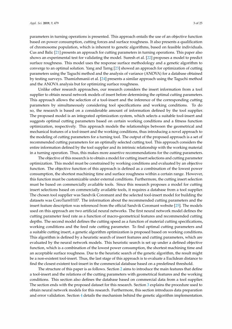
Turning is a process to remove material, which is mainly oriented to metal machining. Within thisfield, several criteria are used to establish the conditions for an acceptable turning process, includingsurface roughness, measurement tolerance, power consumption, machining time, forces, loads, etc.These measurement criteria are highly related to the selected cutting insert, cutting parameters,working material and working conditions [25]. A cutting insert varies according to its geometry, shapeand material composition. Thus, it is possible to apply a specific group of cutting inserts to a specificturning application, working material and working conditions. In general, a tool-insert can be definedby its geometrical features and material composition, which are hereinafter referred as tool-insertfeatures. The most notable tool-insert features are the inscribed circle (ICmm), clearance angle (AN),cutting length (LEmm), corner radius (REmm), thickness (Smm) and shape angle (SC), as shownin Figure 1.

Appl. Sci. 2019, 9 FOR 4

Some concepts, such as individual chromosomes, encoding and decoding procedures and fitness

function, are introduced in this section. Section 5 aims to explain how to use this model for practical

applications in more detail. Examples of applications shown in this section include light roughing

machining, heavy roughing machining and finishing operations. Section 6 summarizes this paper.

2. Datasets Description and Preparation

Turning is a process to remove material, which is mainly oriented to metal machining. Within

this field, several criteria are used to establish the conditions for an acceptable turning process,

including surface roughness, measurement tolerance, power consumption, machining time, forces,

loads, etc. These measurement criteria are highly related to the selected cutting insert, cutting

parameters, working material and working conditions [25]. A cutting insert varies according to its

geometry, shape and material composition. Thus, it is possible to apply a specific group of cutting

inserts to a specific turning application, working material and working conditions. In general, a tool-

insert can be defined by its geometrical features and material composition, which are hereinafter

referred as tool-insert features. The most notable tool-insert features are the inscribed circle (ICmm),

clearance angle (AN), cutting length (LEmm), corner radius (REmm), thickness (Smm) and shape

angle (SC), as shown in Figure 1.

Figure 1. Tool-insert features considered in this study [25]; cutting length (LEmm); corner radius (REmm);

thickness (Smm); and shape angle (SC).

The ICmm is a tool-insert feature that is highly related to the insert size. A large insert size

increases the stability performance but oversizing can lead to high production costs. This feature

must be linked with the depth of the cut, the entering angle and the cutting length to be used. The

AN is the angle between the front face of the insert and the vertical axis of the workpiece [25]. This

feature also defines the negative or positive quality of an insert [25]. On the other hand, the REmm

feature is also related to the chip-breaking and cutting forces but it is mainly linked to finished

surfaces. For a set feed rate cutting parameter, the machining yields a certain surface roughness.

Furthermore, the radial forces that push away the insert in the turning machining become the axial

forces as the depth of the cut increases with respect to the radius nose. As a suggestion from the

supplier, the depth of cut should be greater or equal to 32 of the nose radius of the tool-insert [25].

The insert-shape feature is the most tangible feature, which is mainly selected by accessibility

requirements. This feature defines a tool-holder and the depth of cut range in the process. The SC

feature is defined by the nose angle of the tool-insert, which is related to strength and reliability

issues. Large nose angles are stronger but require more machining power. They also increase the

vibration tendency of the machine. On the contrary, small nose angles are weaker and have small

cutting edges but are linked to better surface roughness [25].

The CTPT feature, which describes the cutting operation, is defined by three possible

configurations: Finishing, Medium and Roughing operations. The WEP feature is a logical feature,

which defines if the tool insert has a wiper radius. The GRADE feature describes the material

composition of a tool-insert. Three features are linked to different grade features. These features

describe the distribution of each grade in the range of area applications for ISO group materials. The

introduced features are MC_L (machine condition low), MC_H (machine condition high) and

Figure 1. Tool-insert features considered in this study [25]; cutting length (LEmm); corner radius(REmm); thickness (Smm); and shape angle (SC).

The ICmm is a tool-insert feature that is highly related to the insert size. A large insert sizeincreases the stability performance but oversizing can lead to high production costs. This feature mustbe linked with the depth of the cut, the entering angle and the cutting length to be used. The AN isthe angle between the front face of the insert and the vertical axis of the workpiece [25]. This featurealso defines the negative or positive quality of an insert [25]. On the other hand, the REmm featureis also related to the chip-breaking and cutting forces but it is mainly linked to finished surfaces.For a set feed rate cutting parameter, the machining yields a certain surface roughness. Furthermore,the radial forces that push away the insert in the turning machining become the axial forces as thedepth of the cut increases with respect to the radius nose. As a suggestion from the supplier, the depthof cut should be greater or equal to 2/3 of the nose radius of the tool-insert [25]. The insert-shapefeature is the most tangible feature, which is mainly selected by accessibility requirements. This featuredefines a tool-holder and the depth of cut range in the process. The SC feature is defined by thenose angle of the tool-insert, which is related to strength and reliability issues. Large nose angles arestronger but require more machining power. They also increase the vibration tendency of the machine.On the contrary, small nose angles are weaker and have small cutting edges but are linked to bettersurface roughness [25].

The CTPT feature, which describes the cutting operation, is defined by three possibleconfigurations: Finishing, Medium and Roughing operations. The WEP feature is a logical feature,which defines if the tool insert has a wiper radius. The GRADE feature describes the materialcomposition of a tool-insert. Three features are linked to different grade features. These featuresdescribe the distribution of each grade in the range of area applications for ISO group materials.

Appl. Sci. 2019, 9, 479 5 of 25

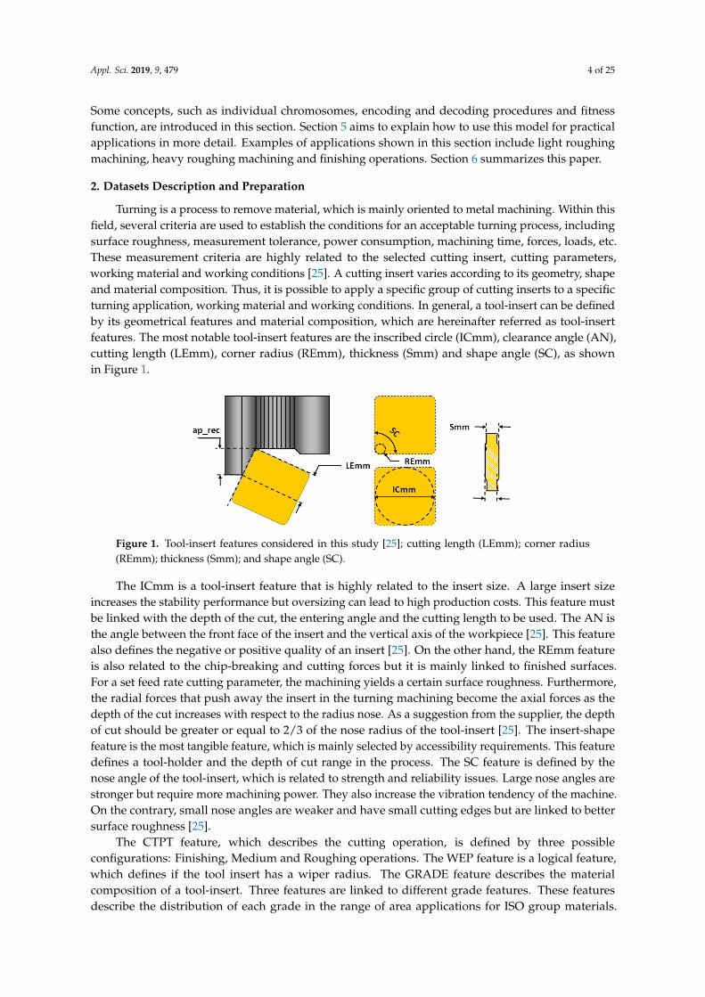
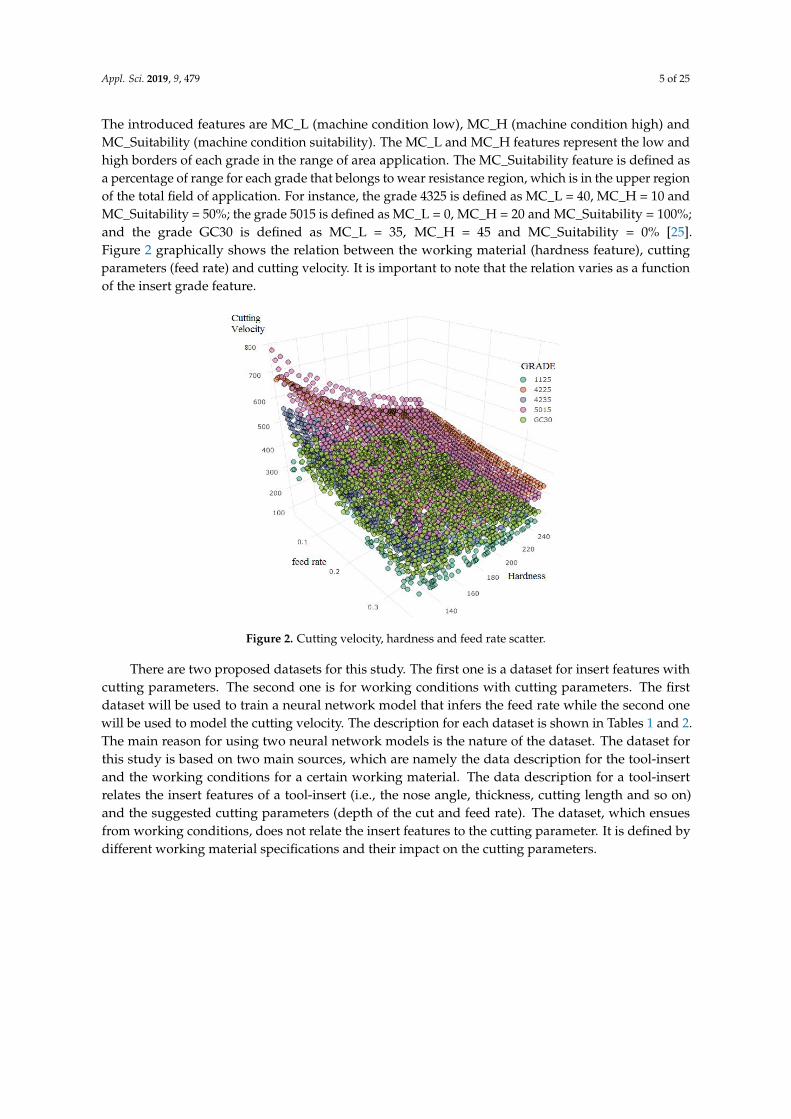
The introduced features are MC_L (machine condition low), MC_H (machine condition high) andMC_Suitability (machine condition suitability). The MC_L and MC_H features represent the low andhigh borders of each grade in the range of area application. The MC_Suitability feature is defined asa percentage of range for each grade that belongs to wear resistance region, which is in the upper regionof the total field of application. For instance, the grade 4325 is defined as MC_L = 40, MC_H = 10 andMC_Suitability = 50%; the grade 5015 is defined as MC_L = 0, MC_H = 20 and MC_Suitability = 100%;and the grade GC30 is defined as MC_L = 35, MC_H = 45 and MC_Suitability = 0% [25].Figure 2 graphically shows the relation between the working material (hardness feature), cuttingparameters (feed rate) and cutting velocity. It is important to note that the relation varies as a functionof the insert grade feature.


MC_Suitability (machine condition suitability). The MC_L and MC_H features represent the low and

high borders of each grade in the range of area application. The MC_Suitability feature is defined as

a percentage of range for each grade that belongs to wear resistance region, which is in the upper

region of the total field of application. For instance, the grade 4325 is defined as MC_L = 40, MC_H =

10 and MC_Suitability = 50%; the grade 5015 is defined as MC_L = 0, MC_H = 20 and MC_Suitability

= 100%; and the grade GC30 is defined as MC_L = 35, MC_H = 45 and MC_Suitability = 0% [25]. Figure

2 graphically shows the relation between the working material (hardness feature), cutting parameters

(feed rate) and cutting velocity. It is important to note that the relation varies as a function of the

insert grade feature.

Figure 2. Cutting velocity, hardness and feed rate scatter.

There are two proposed datasets for this study. The first one is a dataset for insert features with

cutting parameters. The second one is for working conditions with cutting parameters. The first

dataset will be used to train a neural network model that infers the feed rate while the second one

will be used to model the cutting velocity. The description for each dataset is shown in Table 1 and

Table 2. The main reason for using two neural network models is the nature of the dataset. The dataset

for this study is based on two main sources, which are namely the data description for the tool-insert

and the working conditions for a certain working material. The data description for a tool-insert

relates the insert features of a tool-insert (i.e., the nose angle, thickness, cutting length and so on) and

the suggested cutting parameters (depth of the cut and feed rate). The dataset, which ensues from

working conditions, does not relate the insert features to the cutting parameter. It is defined by

different working material specifications and their impact on the cutting parameters.

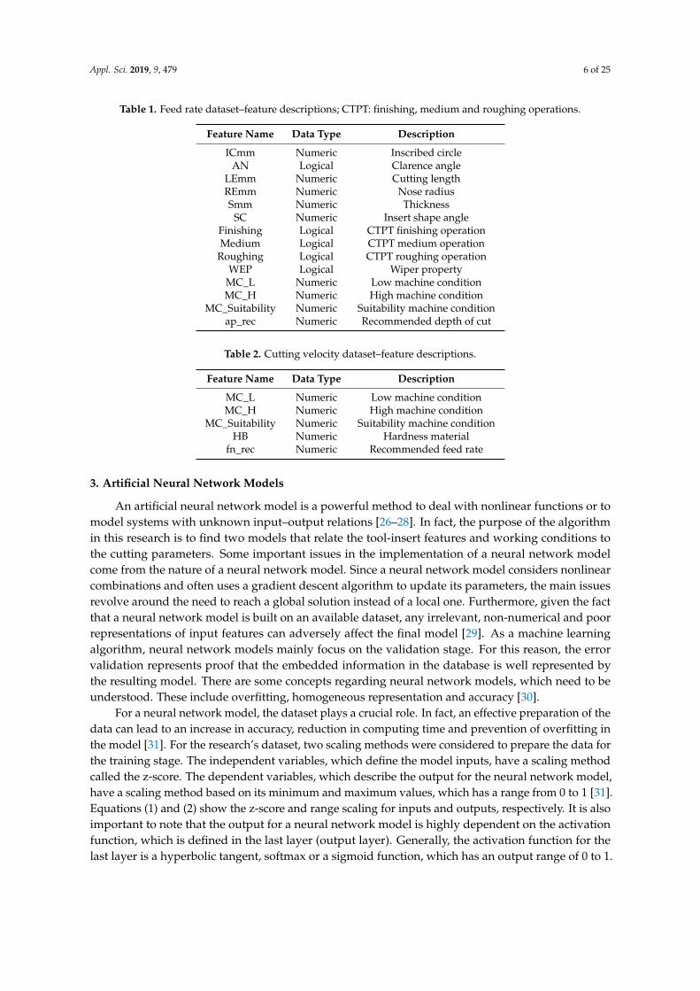
Table 1. Feed rate dataset – feature descriptions; CTPT: finishing, medium and roughing operations.

Feature Name Data Type Description

ICmm Numeric Inscribed circle

AN Logical Clarence angle

LEmm Numeric Cutting length

REmm Numeric Nose radius

Smm Numeric Thickness

SC Numeric Insert shape angle

Finishing Logical CTPT finishing operation

Medium Logical CTPT medium operation

Roughing Logical CTPT roughing operation

Figure 2. Cutting velocity, hardness and feed rate scatter.

There are two proposed datasets for this study. The first one is a dataset for insert features withcutting parameters. The second one is for working conditions with cutting parameters. The firstdataset will be used to train a neural network model that infers the feed rate while the second onewill be used to model the cutting velocity. The description for each dataset is shown in Tables 1 and 2.The main reason for using two neural network models is the nature of the dataset. The dataset forthis study is based on two main sources, which are namely the data description for the tool-insertand the working conditions for a certain working material. The data description for a tool-insertrelates the insert features of a tool-insert (i.e., the nose angle, thickness, cutting length and so on)and the suggested cutting parameters (depth of the cut and feed rate). The dataset, which ensuesfrom working conditions, does not relate the insert features to the cutting parameter. It is defined bydifferent working material specifications and their impact on the cutting parameters.

Appl. Sci. 2019, 9, 479 6 of 25

Table 1. Feed rate dataset–feature descriptions; CTPT: finishing, medium and roughing operations.


ICmm Numeric Inscribed circleAN Logical Clarence angle

LEmm Numeric Cutting lengthREmm Numeric Nose radiusSmm Numeric Thickness

SC Numeric Insert shape angleFinishing Logical CTPT finishing operationMedium Logical CTPT medium operation

Roughing Logical CTPT roughing operationWEP Logical Wiper property

MC_L Numeric Low machine conditionMC_H Numeric High machine condition

MC_Suitability Numeric Suitability machine conditionap_rec Numeric Recommended depth of cut

Table 2. Cutting velocity dataset–feature descriptions.


MC_L Numeric Low machine conditionMC_H Numeric High machine condition

MC_Suitability Numeric Suitability machine conditionHB Numeric Hardness material

fn_rec Numeric Recommended feed rate

3. Artificial Neural Network Models

An artificial neural network model is a powerful method to deal with nonlinear functions or tomodel systems with unknown input–output relations [26–28]. In fact, the purpose of the algorithmin this research is to find two models that relate the tool-insert features and working conditions tothe cutting parameters. Some important issues in the implementation of a neural network modelcome from the nature of a neural network model. Since a neural network model considers nonlinearcombinations and often uses a gradient descent algorithm to update its parameters, the main issuesrevolve around the need to reach a global solution instead of a local one. Furthermore, given the factthat a neural network model is built on an available dataset, any irrelevant, non-numerical and poorrepresentations of input features can adversely affect the final model [29]. As a machine learningalgorithm, neural network models mainly focus on the validation stage. For this reason, the errorvalidation represents proof that the embedded information in the database is well represented bythe resulting model. There are some concepts regarding neural network models, which need to beunderstood. These include overfitting, homogeneous representation and accuracy [30].

For a neural network model, the dataset plays a crucial role. In fact, an effective preparation of thedata can lead to an increase in accuracy, reduction in computing time and prevention of overfitting inthe model [31]. For the research’s dataset, two scaling methods were considered to prepare the data forthe training stage. The independent variables, which define the model inputs, have a scaling methodcalled the z-score. The dependent variables, which describe the output for the neural network model,have a scaling method based on its minimum and maximum values, which has a range from 0 to 1 [31].Equations (1) and (2) show the z-score and range scaling for inputs and outputs, respectively. It is alsoimportant to note that the output for a neural network model is highly dependent on the activationfunction, which is defined in the last layer (output layer). Generally, the activation function for thelast layer is a hyperbolic tangent, softmax or a sigmoid function, which has an output range of 0 to 1.

Appl. Sci. 2019, 9, 479 7 of 25

Other activation functions are widely used for neural network models although this research usesa linear function because it can be easily implemented with less computational burden.

xi−scaled =xi −mean(x)

σ(x)(1)

yi−scaled =yi −min(y)

max(y)−min(y)(2)

The architecture and error validation of a neural network model are closely linked with each other.In fact, the performance of a neural network model is defined by its architecture, but this last one isselected by error validation. The architecture refers to the set of parameters that govern the complexityof the model, including the number of neurons, layers, updating and regularization algorithms amongothers. The error validation refers to an evaluation procedure for a certain architecture to find a balancebetween accuracy and error distribution without causing overfitting [32]. In practical applications,the training and testing datasets are used to achieve an architecture model that represents almostall information in the dataset. The training data are used to teach the model on the input–outputrelations. The testing data validate the model so it represents most of the total spectrum of possibilitiesin the dataset. For the present research, the databases for the feed rate and cutting velocity model,which are described in Tables 1 and 2, are divided into a ratio of 0.5 for training and testing validation.The algorithm for converging the weights in a neural network model also plays an important rolein the architecture. For this implementation, a globally convergent training scheme, based on theresilient propagation, is used. A crucial advantage of this algorithm compared to the traditionalback-propagation or normal resilient propagation is the computing time. This approach shows betteraccuracy performance with similar datasets to be used for this research (datasets that are compoundedby factors and numerical mapped values [29]).

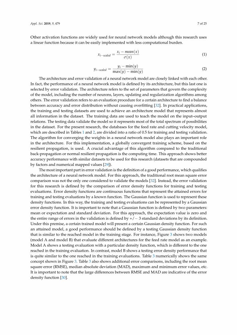
The most important part in error validation is the definition of a good performance, which qualifiesthe architecture of a neural network model. For this approach, the traditional root mean square errorcomparison was not the only one considered to validate the models [32]. Instead, the error validationfor this research is defined by the comparison of error density functions for training and testingevaluations. Error density functions are continuous functions that represent the attained errors fortraining and testing evaluations by a known function. The Gaussian function is used to represent thesedensity functions. In this way, the training and testing evaluations can be represented by a Gaussianerror density function. It is important to note that a Gaussian function is defined by two parameters:mean or expectation and standard deviation. For this approach, the expectation value is zero andthe entire range of errors in the validation is defined by +/− 3 standard deviations by its definition.Under this premise, a certain trained model will present a certain Gaussian density function. For suchan attained model, a good performance should be defined by a testing Gaussian density functionthat is similar to the reached model in the training stage. For instance, Figure 3 shows two models(model A and model B) that evaluate different architectures for the feed rate model as an example.Model A shows a testing evaluation with a particular density function, which is different to the onereached in the training evaluation. In contrast, model B shows a testing error density performance thatis quite similar to the one reached in the training evaluations. Table 3 numerically shows the sameconcept shown in Figure 3. Table 3 also shows additional error comparisons, including the root meansquare error (RMSE), median absolute deviation (MAD), maximum and minimum error values, etc.It is important to note that the large differences between RMSE and MAD are indicative of the errordensity function [30].

Appl. Sci. 2019, 9, 479 8 of 25


algorithms among others. The error validation refers to an evaluation procedure for a certain

architecture to find a balance between accuracy and error distribution without causing overfitting

[32]. In practical applications, the training and testing datasets are used to achieve an architecture

model that represents almost all information in the dataset. The training data are used to teach the

model on the input–output relations. The testing data validate the model so it represents most of the

total spectrum of possibilities in the dataset. For the present research, the databases for the feed rate

and cutting velocity model, which are described in Table 1 and Table 2, are divided into a ratio of 0.5

for training and testing validation. The algorithm for converging the weights in a neural network

model also plays an important role in the architecture. For this implementation, a globally convergent

training scheme, based on the resilient propagation, is used. A crucial advantage of this algorithm

compared to the traditional back-propagation or normal resilient propagation is the computing time.

This approach shows better accuracy performance with similar datasets to be used for this research

(datasets that are compounded by factors and numerical mapped values [29]).

The most important part in error validation is the definition of a good performance, which

qualifies the architecture of a neural network model. For this approach, the traditional root mean

square error comparison was not the only one considered to validate the models [32]. Instead, the

error validation for this research is defined by the comparison of error density functions for training

and testing evaluations. Error density functions are continuous functions that represent the attained

errors for training and testing evaluations by a known function. The Gaussian function is used to

represent these density functions. In this way, the training and testing evaluations can be represented

by a Gaussian error density function. It is important to note that a Gaussian function is defined by

two parameters: mean or expectation and standard deviation. For this approach, the expectation

value is zero and the entire range of errors in the validation is defined by +/− 3 standard deviations

by its definition. Under this premise, a certain trained model will present a certain Gaussian density

function. For such an attained model, a good performance should be defined by a testing Gaussian

density function that is similar to the reached model in the training stage. For instance, Figure 3 shows

two models (model A and model B) that evaluate different architectures for the feed rate model as an

example. Model A shows a testing evaluation with a particular density function, which is different

to the one reached in the training evaluation. In contrast, model B shows a testing error density

performance that is quite similar to the one reached in the training evaluations. Table 3 numerically

shows the same concept shown in Figure 3. Table 3 also shows additional error comparisons,

including the root mean square error (RMSE), median absolute deviation (MAD), maximum and

minimum error values, etc. It is important to note that the large differences between RMSE and MAD

are indicative of the error density function [30].

Figure 3. Example of error density function comparison.

Table 3. Error validation example.

Properties

Model A Model B

Training

Data

Testing

Data

Training

Data

Testing

Data

Mean square error 11.9 × 10–4 5.8 × 10–4 7.8 × 10–4 6.7 × 10–4

Root mean square error 34.5 × 10–3 24.2 × 10–3 28.0 × 10–3 25.9 × 10–3

Figure 3. Example of error density function comparison.

Table 3. Error validation example.

Properties Model A Model B

Training Data Testing Data Training Data Testing Data

Mean square error 11.9 × 10−4 5.8 × 10−4 7.8 × 10−4 6.7 × 10−4

Root mean square error 34.5 × 10−3 24.2 × 10−3 28.0 × 10−3 25.9 × 10−3

Median absolute deviation 22.4 × 10−3 16.7 × 10−3 18.2 × 10−3 16.7 × 10−3

Max. value 0.1275 0.0811 0.0698 0.0675Min. value −0.1167 −0.0791 −0.0828 −0.0828

Mean 19.4 × 10−5 87.0 × 10−5 −8.0 × 10−4 −1.8 × 10−4

Standard deviation 34.5 × 10−3 24.2 × 10−3 28.0 × 10−3 26.0 × 10−3

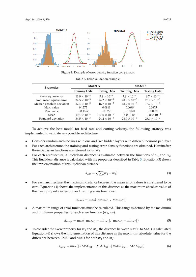
To achieve the best model for feed rate and cutting velocity, the following strategy wasimplemented to validate any possible architecture:

• Consider random architectures with one and two hidden layers with different neurons per layer.• For each architecture, the training and testing error density functions are obtained. Hereinafter,

these Gaussian functions are referred as m1, m2

• For each architecture, a Euclidean distance is evaluated between the functions of m1 and m2.This Euclidean distance is calculated with the properties described in Table 3. Equation (3) showsthe implementation of this Euclidean distance:

dED =√

∑(m1 −m2) (3)

• For each architecture, the maximum distance between the mean error values is considered to bezero. Equation (4) shows the implementation of this distance as the maximum absolute value ofthe mean property in testing and training error functions:

dmean = max(|meanm1| , |meanm2| ) (4)

• A maximum range of error functions must be calculated. This range is defined by the maximumand minimum properties for each error function (m1, m2).

drange = max(|maxm1 −minm1| , |maxm2 −minm2| ) (5)

• To consider the skew property for m1 and m2, the distance between RMSE to MAD is calculated.Equation (6) shows the implementation of this distance as the maximum absolute value for thedifference between RMSE and MAD for both m1 and m2:

dskew = max(|RMSEm1 −MADm1| , |RMSEm2 −MADm2| ) (6)

Appl. Sci. 2019, 9, 479 9 of 25

• After this, the performance of a suggested model is given by Equation (7), which evaluates theEuclidean distance, mean distance to zero, the total error range and skew distance as a function ofm1 and m2. The constant k allows the function to be adjusted to a certain range of values, which isshown as follows:

Fper f o(m1, m2) =k

dED · dmean · drange · dskew(7)

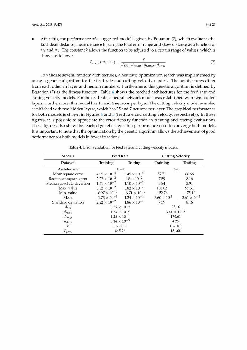
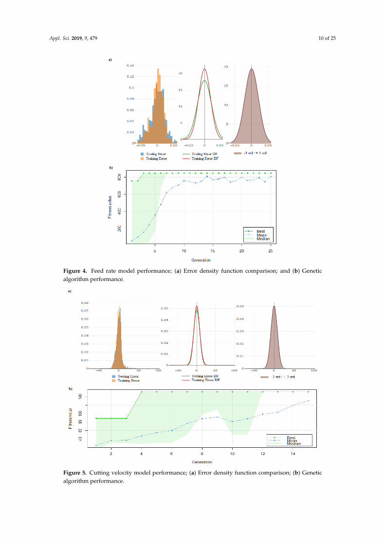
To validate several random architectures, a heuristic optimization search was implemented byusing a genetic algorithm for the feed rate and cutting velocity models. The architectures differfrom each other in layer and neuron numbers. Furthermore, this genetic algorithm is defined byEquation (7) as the fitness function. Table 4 shows the reached architectures for the feed rate andcutting velocity models. For the feed rate, a neural network model was established with two hiddenlayers. Furthermore, this model has 15 and 4 neurons per layer. The cutting velocity model was alsoestablished with two hidden layers, which has 25 and 7 neurons per layer. The graphical performancefor both models is shown in Figures 4 and 5 (feed rate and cutting velocity, respectively). In thesefigures, it is possible to appreciate the error density function in training and testing evaluations.These figures also show the reached genetic algorithm performance used to converge both models.It is important to note that the optimization by the genetic algorithm allows the achievement of goodperformance for both models in fewer iterations.

Table 4. Error validation for feed rate and cutting velocity models.

Models Feed Rate Cutting Velocity

Datasets Training Testing Training Testing

Architecture 15–4 15–5Mean square error 4.95 × 10−4 3.45 × 10−4 57.71 66.66

Root mean square error 2.22 × 10−2 1.8 × 10−2 7.59 8.16Median absolute deviation 1.41 × 10−2 1.10 × 10−2 3.84 3.91

Max. value 5.82 × 10−2 5.82 × 10−2 102.82 95.51Min. value −6.97 × 10−2 −6.71 × 10−2 −52.76 −75.10

Mean −1.73 × 10−4 1.24 × 10−4 −3.60 × 10-2 −3.61 × 10-2

Standard deviation 2.22 × 10−2 1.86 × 10−2 7.59 8.16dED 6.55 × 10−3 25.16

dmean 1.73 × 10−3 3.61 × 10−2

drange 1.28 × 10−1 170.61dskew 8.14 × 10−3 4.25

k 1 × 10−5 1 × 105

Fperfo 845.26 151.68

Appl. Sci. 2019, 9, 479 10 of 25


Table 4. Error validation for feed rate and cutting velocity models.

Models Feed Rate Cutting Velocity

Datasets Training Testing Training Testing

Architecture 15–4 15–5

Mean square error 4.95 × 10–4 3.45 × 10–4 57.71 66.66

Root mean square error 2.22 × 10–2 1.8 × 10–2 7.59 8.16

Median absolute deviation 1.41 × 10–2 1.10 × 10–2 3.84 3.91

Max. value 5.82 × 10–2 5.82 × 10–2 102.82 95.51

Min. value –6.97 × 10–2 –6.71 × 10–2 –52.76 –75.10

Mean –1.73 × 10–4 1.24 × 10–4 –3.60 × 10-2 –3.61 × 10-2

Standard deviation 2.22 × 10–2 1.86 × 10–2 7.59 8.16

EDd 6.55 × 10–3 25.16

meand 1.73 × 10–3 3.61 × 10–2

ranged 1.28 × 10–1 170.61

skewd 8.14 × 10–3 4.25

k 1 × 10–5 1 × 105

perfoF 845.26 151.68

Figure 4. Feed rate model performance; (a) Error density function comparison; and (b) Genetic algorithm

performance.

Figure 4. Feed rate model performance; (a) Error density function comparison; and (b) Geneticalgorithm performance.Appl. Sci. 2019, 9 FOR 10

Figure 5. Cutting velocity model performance; (a) Error density function comparison; (b) Genetic algorithm

performance.

4. Genetic Algorithm Optimization

A genetic algorithm (GA) is a heuristic search algorithm inspired by evolutionary mechanisms

and biological natural selection. This algorithm defines a searching space of solutions and allows us

to find individual solutions, which satisfy a certain condition. This condition is usually referred to as

the fitness function [33]. This study aims to define a heuristic search based on GA, which allows us

to find an optimal insert-tool for certain working specifications. This insert-tool search is governed

by a fitness function, which is defined by a combination of the lowest power consumption, the

shortest machining time and acceptable surface roughness among others. Figure 6 shows a general

scheme of the proposed GA implementation for this research. Initially, it can be appreciated that the

feed rate model evaluates the GA chromosome. After this, the feed rate and working conditions can

be used as the inputs for the cutting velocity model. The resulting feed rate and cutting velocity are

evaluated by the GA fitness function, which assess the current chromosome along with the working

specifications. Finally, the GA operations transform the current population to the next generation.

According to their characteristics, the individuals in the population improve with each iteration.

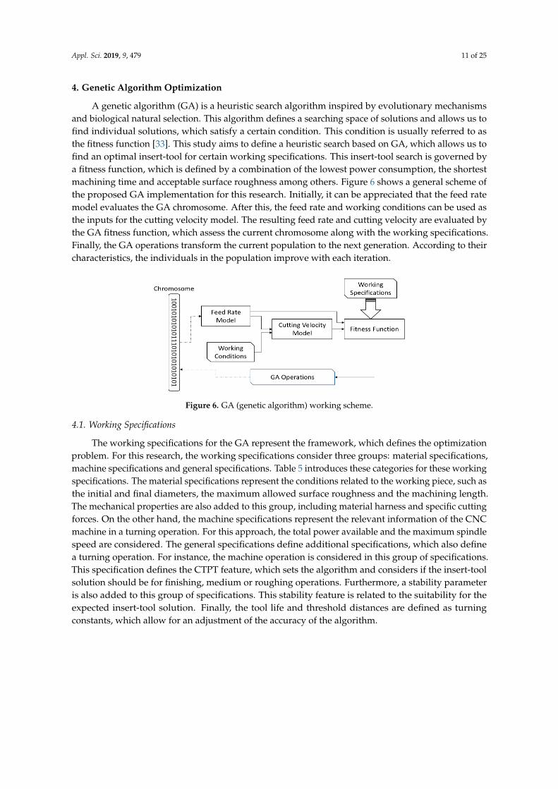
Figure 6. GA (genetic algorithm) working scheme.

Figure 5. Cutting velocity model performance; (a) Error density function comparison; (b) Geneticalgorithm performance.

Appl. Sci. 2019, 9, 479 11 of 25


A genetic algorithm (GA) is a heuristic search algorithm inspired by evolutionary mechanismsand biological natural selection. This algorithm defines a searching space of solutions and allows us tofind individual solutions, which satisfy a certain condition. This condition is usually referred to asthe fitness function [33]. This study aims to define a heuristic search based on GA, which allows us tofind an optimal insert-tool for certain working specifications. This insert-tool search is governed bya fitness function, which is defined by a combination of the lowest power consumption, the shortestmachining time and acceptable surface roughness among others. Figure 6 shows a general scheme ofthe proposed GA implementation for this research. Initially, it can be appreciated that the feed ratemodel evaluates the GA chromosome. After this, the feed rate and working conditions can be used asthe inputs for the cutting velocity model. The resulting feed rate and cutting velocity are evaluated bythe GA fitness function, which assess the current chromosome along with the working specifications.Finally, the GA operations transform the current population to the next generation. According to theircharacteristics, the individuals in the population improve with each iteration.


Figure 5. Cutting velocity model performance; (a) Error density function comparison; (b) Genetic algorithm

performance.


A genetic algorithm (GA) is a heuristic search algorithm inspired by evolutionary mechanisms

and biological natural selection. This algorithm defines a searching space of solutions and allows us

to find individual solutions, which satisfy a certain condition. This condition is usually referred to as

the fitness function [33]. This study aims to define a heuristic search based on GA, which allows us

to find an optimal insert-tool for certain working specifications. This insert-tool search is governed

by a fitness function, which is defined by a combination of the lowest power consumption, the

shortest machining time and acceptable surface roughness among others. Figure 6 shows a general

scheme of the proposed GA implementation for this research. Initially, it can be appreciated that the

feed rate model evaluates the GA chromosome. After this, the feed rate and working conditions can

be used as the inputs for the cutting velocity model. The resulting feed rate and cutting velocity are

evaluated by the GA fitness function, which assess the current chromosome along with the working

specifications. Finally, the GA operations transform the current population to the next generation.

According to their characteristics, the individuals in the population improve with each iteration.

Figure 6. GA (genetic algorithm) working scheme. Figure 6. GA (genetic algorithm) working scheme.

4.1. Working Specifications

The working specifications for the GA represent the framework, which defines the optimizationproblem. For this research, the working specifications consider three groups: material specifications,machine specifications and general specifications. Table 5 introduces these categories for these workingspecifications. The material specifications represent the conditions related to the working piece, such asthe initial and final diameters, the maximum allowed surface roughness and the machining length.The mechanical properties are also added to this group, including material harness and specific cuttingforces. On the other hand, the machine specifications represent the relevant information of the CNCmachine in a turning operation. For this approach, the total power available and the maximum spindlespeed are considered. The general specifications define additional specifications, which also definea turning operation. For instance, the machine operation is considered in this group of specifications.This specification defines the CTPT feature, which sets the algorithm and considers if the insert-toolsolution should be for finishing, medium or roughing operations. Furthermore, a stability parameteris also added to this group of specifications. This stability feature is related to the suitability for theexpected insert-tool solution. Finally, the tool life and threshold distances are defined as turningconstants, which allow for an adjustment of the accuracy of the algorithm.

Appl. Sci. 2019, 9, 479 12 of 25

Table 5. Working specifications.

Material specifications

Initial diameter Di Numeric valuesFinal diameter Df Numeric values

Machining length Lm Numeric valuesHardness HB Numeric values

Specific cutting force Kc Numeric valuesMax. surface roughness Ra_max Numeric values

Machine specifications

Main motor power Pnet Numeric valuesMax. spindle speed nmax Numeric values

General specifications

Machine operation CTPT Finishing–Medium–RoughingStability / Excellent–Good–PoorToot life Tlife Numeric values

Threshold distance Thd Numeric values

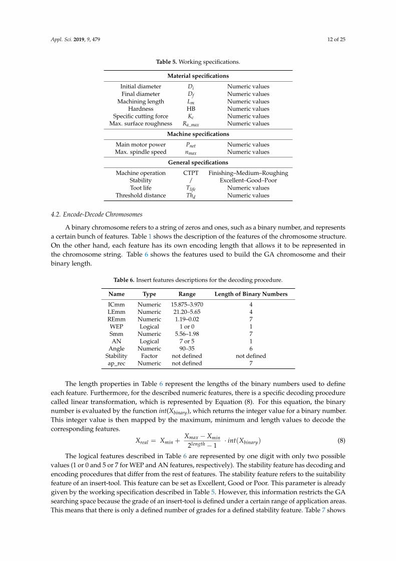
4.2. Encode-Decode Chromosomes

A binary chromosome refers to a string of zeros and ones, such as a binary number, and representsa certain bunch of features. Table 1 shows the description of the features of the chromosome structure.On the other hand, each feature has its own encoding length that allows it to be represented inthe chromosome string. Table 6 shows the features used to build the GA chromosome and theirbinary length.

Table 6. Insert features descriptions for the decoding procedure.

Name Type Range Length of Binary Numbers

ICmm Numeric 15.875–3.970 4LEmm Numeric 21.20–5.65 4REmm Numeric 1.19–0.02 7WEP Logical 1 or 0 1Smm Numeric 5.56–1.98 7AN Logical 7 or 5 1

Angle Numeric 90–35 6Stability Factor not defined not definedap_rec Numeric not defined 7

The length properties in Table 6 represent the lengths of the binary numbers used to defineeach feature. Furthermore, for the described numeric features, there is a specific decoding procedurecalled linear transformation, which is represented by Equation (8). For this equation, the binarynumber is evaluated by the function int(Xbinary), which returns the integer value for a binary number.This integer value is then mapped by the maximum, minimum and length values to decode thecorresponding features.

Xreal = Xmin +Xmax − Xmin

2length − 1· int(Xbinary) (8)

The logical features described in Table 6 are represented by one digit with only two possiblevalues (1 or 0 and 5 or 7 for WEP and AN features, respectively). The stability feature has decoding andencoding procedures that differ from the rest of features. The stability feature refers to the suitabilityfeature of an insert-tool. This feature can be set as Excellent, Good or Poor. This parameter is alreadygiven by the working specification described in Table 5. However, this information restricts the GAsearching space because the grade of an insert-tool is defined under a certain range of application areas.This means that there is only a defined number of grades for a defined stability feature. Table 7 shows

Appl. Sci. 2019, 9, 479 13 of 25

the stability condition associated with the insert-tool grades in the present dataset. Under this premise,a grades list (indexed list) and a binary number define the proposed encoding procedure for thefeatures’ stability. The binary number indexes the position for each grade on such list. For instance,we considered the stability “Good” described in Table 8. Since there are only four possible gradesin this condition, the binary number to encode this feature is a string of three digits (000, 001, 010,011, 111, etc.). Thus, the number of ones in such binary number represents the index in the grade list.For two ones in the binary number, the grade is 4225 and for 0 ones in the binary number, the grade is1125, etc.

Table 7. Grade stability.

GRADE Suitability Stability GRADE Suitability Stability

1125 75% Good 4305 100% Excellent1515 75% Good 4315 83.3% Excellent1525 100% Excellent 4325 50% Good235 0% Poor 4335 16.6% Poor

4215 83.3% Excellent 5015 100% Excellent4225 50% Good GC15 100% Excellent4235 20% Poor GC30 0% Poor

Table 8. Indexed list for good stability.

Index Grade Stability

0 1125 Good1 1515 Good2 4225 Good3 4325 Good

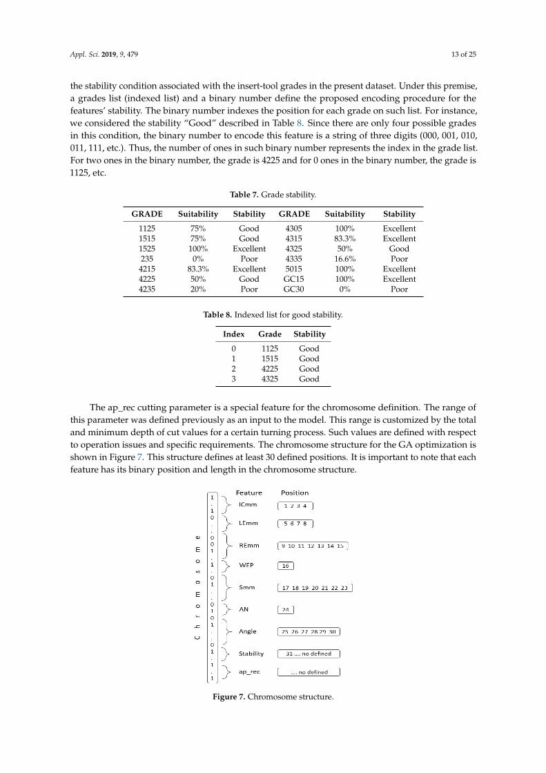
The ap_rec cutting parameter is a special feature for the chromosome definition. The range ofthis parameter was defined previously as an input to the model. This range is customized by the totaland minimum depth of cut values for a certain turning process. Such values are defined with respectto operation issues and specific requirements. The chromosome structure for the GA optimization isshown in Figure 7. This structure defines at least 30 defined positions. It is important to note that eachfeature has its binary position and length in the chromosome structure.


shown in Figure 7. This structure defines at least 30 defined positions. It is important to note that each

feature has its binary position and length in the chromosome structure.

Figure 7. Chromosome structure.

4.3. Fitness Function Definition

The fitness function is the main concern for the development of the GA and its definition

establishes the expected output of the algorithm. For this research, this function was defined as a

function that evaluates the lowest power consumption, the shortest machining time and an

acceptable surface roughness among others. Equation (9) defines the fitness function for this genetic

algorithm optimization. This equation is a summation of goal functions ig , which evaluate power

consumption, machining time, surface roughness, etc. Furthermore, each ig function is weighted

by a constant

i , which allows the adjustment of the importance of each ig function.

i

i

i gfitness =

(9)

The goal function, 1g , described in Equation (10), evaluates the power consumption ratio in the

turning process. This function uses Equation (11) to evaluate the theoretical power consumption, P

[20]. Furthermore, the netP constant is the total available power in the machine (introduced in Table

5). The constant allows for the consideration of the friction losses in the transmission motor [20]

although this constant is equal to 1 for this research. Equation (12) shows the cutting force, cF , as a

function of the specific cutting force, cK , related to the working material, depth of cut ( recap _ ) and

feed rate ( recfn _ ) [25]. It is important to note that the specific cutting force, cK , is a parameter that

was also introduced in Table 5.

P

Pg net=

1

(10)

4106

= cc Fv

P

(11)

recfnrecapKF cc __ = (12)

The goal function, 2g , described in Equation (13), defines the machining time ratio, which

relates the tool life to the machining time. The tool life, lifeT , is a tool supplier parameter, which

defines the approximate tool life for a tool-insert. The machining time is an objective variable

Figure 7. Chromosome structure.

Appl. Sci. 2019, 9, 479 14 of 25

4.3. Fitness Function Definition

The fitness function is the main concern for the development of the GA and its definitionestablishes the expected output of the algorithm. For this research, this function was defined asa function that evaluates the lowest power consumption, the shortest machining time and an acceptablesurface roughness among others. Equation (9) defines the fitness function for this genetic algorithmoptimization. This equation is a summation of goal functions gi, which evaluate power consumption,machining time, surface roughness, etc. Furthermore, each gi function is weighted by a constant ωi,which allows the adjustment of the importance of each gi function.

f itness = ∑i

ωi · gi (9)

The goal function, g1, described in Equation (10), evaluates the power consumption ratio in theturning process. This function uses Equation (11) to evaluate the theoretical power consumption, P [20].Furthermore, the Pnet constant is the total available power in the machine (introduced in Table 5).The constant γ allows for the consideration of the friction losses in the transmission motor [20] althoughthis constant is equal to 1 for this research. Equation (12) shows the cutting force, Fc, as a functionof the specific cutting force, Kc, related to the working material, depth of cut (ap_rec) and feed rate(fn_rec) [25]. It is important to note that the specific cutting force, Kc, is a parameter that was alsointroduced in Table 5.

g1 =γ · Pnet

P(10)

P =vc · Fc

6× 104 (11)

Fc = Kc · ap_rec · f n_rec (12)

The goal function, g2, described in Equation (13), defines the machining time ratio, which relatesthe tool life to the machining time. The tool life, Tlife, is a tool supplier parameter, which definesthe approximate tool life for a tool-insert. The machining time is an objective variable evaluated inEquation (14). This defines the machining time in the turning process with a certain group of cuttingparameters. Equation (15) presents the spindle speed, n, as a function of the cutting velocity, vc andthe current machining diameter, D. It is important to note that n varies according to D. Thus, for eachmachining pass (diameter decreasing), the spindle speed increases.

g2 =Tli f e

Tm(13)

Tm =Lm

f n_rec · n (14)

n =vc × 1000

π · D (15)

The goal function, g3, defined in Equation (16), relates the maximum surface roughness, Ra_max,to the theoretically reached surface roughness, Ra. The parameter Ra_max is a working specificationof material that defines the maximum allowed roughness. Ra is an objective variable defined inEquation (17), which estimates the surface roughness for a certain finishing operation [20].

g3 =Ra_max

Ra(16)

Ra =125 · f n_rec2

REmm(17)

Appl. Sci. 2019, 9, 479 15 of 25

The goal function, g4, defined in Equation (18), relates the objective variable, deuclidean, to theparameter Thd (threshold distance). The variable deuclidean is obtained by Equation (19). This equationcalculates the Euclidean distance between the features xi and yi, which are defined by the suggestedGA tool-insert features and the nth tool-insert in the dataset, respectively.

g4 =Thd

deuclidean(18)

deuclidean =√

∑i(xi − yi)

2 (19)

The goal function, g5, shown in Equation (20), evaluates the spindle speed ratio, which is used inthe turning process. This objective function relates the maximum spindle speed of the machine to thetheoretical spindle speed reached in the turning process.

g5 =nmax

n(20)

The goal function, g6, shown in Equation (21), evaluates the suitability range for a certain insertgrade. This function assesses if a suggested grade is more appropriate for a specific application areacompared to other solutions. Grades that are more specific are preferred instead of the general grades.

g6 =1

MC_H −MC_L(21)

Overall, there are two fitness functions regarding the turning processes: the finishing or roughingoperations. In fact, for the roughing operation, the surface roughness is not considered in the fitnessfunction, but the power consumption, machining time, Euclidean distance, spindle speed ratio andsuitability are considered. For the finishing process, the fitness function considers the surface roughness,Euclidean distance and suitability grade. Equations (22) and (23) show the proposed fitness functionfor the roughing and finishing operations.

froughing = ω1Pnet

P+ ω2

Tli f e

Tm+ ω3

Thddeucliden

+ ω4nmax

n51

MC_H−MC_L(22)

f f inishing = ω1Ra_max

Ra2Thd

deucliden 31

MC_H−MC_L

(23)

4.4. Boundary Constraints

The boundary constraints for the GA optimization define the searching space for the algorithm.These boundary constraints allow us to control the chromosome evolution and ensure that thealgorithm is converging towards a suitable solution. The first mechanism for controlling the populationevolution is called the feasible solution control. This boundary control prevents infeasible individualsfrom appearing in the population [20]. This mechanism evaluates the goal function, g4, by theconstraint mentioned in Equation (24). Thus, only similar insert-tools are chosen as part of thepopulation. The infeasible solutions are not considered.

g4 =Thd

deuclidean> 1 (24)

Some boundary constraints are established to prevent solutions that evaluate a parameter outsideof the machine capabilities. For example, the expression mentioned in Equation (25) avoids GAindividuals when evaluating power consumption, which exceeds the maximum power of the machine.

Appl. Sci. 2019, 9, 479 16 of 25

The constraint mentioned in Equation (26) avoids solutions that need spindle speeds greater than themaximum defined speed for the machine.

g1 =γ · Pnet

P> 1 (25)

g5 =nmax

n(26)

5. Application Examples

This section aims to explain some applications for the algorithm described in this research.Three application examples are used to show the performance and results of the proposed approach.These examples are defined under different working conditions and fitness functions.

5.1. Light Roughing Operation

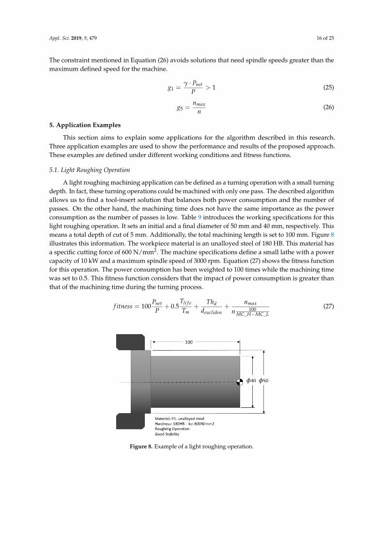
A light roughing machining application can be defined as a turning operation with a small turningdepth. In fact, these turning operations could be machined with only one pass. The described algorithmallows us to find a tool-insert solution that balances both power consumption and the number ofpasses. On the other hand, the machining time does not have the same importance as the powerconsumption as the number of passes is low. Table 9 introduces the working specifications for thislight roughing operation. It sets an initial and a final diameter of 50 mm and 40 mm, respectively. Thismeans a total depth of cut of 5 mm. Additionally, the total machining length is set to 100 mm. Figure 8illustrates this information. The workpiece material is an unalloyed steel of 180 HB. This material hasa specific cutting force of 600 N/mm2. The machine specifications define a small lathe with a powercapacity of 10 kW and a maximum spindle speed of 3000 rpm. Equation (27) shows the fitness functionfor this operation. The power consumption has been weighted to 100 times while the machining timewas set to 0.5. This fitness function considers that the impact of power consumption is greater thanthat of the machining time during the turning process.

f itness = 100Pnet

P+ 0.5

Tli f e

Tm+

Thddeucliden

+nmax

n 100MC_H−MC_L

(27)


Figure 8. Example of a light roughing operation.

Table 9. Working specifications of the light roughing operation example.

Material Specifications

Initial diameter iD 50 mm

Final diameter fD 40 mm

Machining length mL 100 mm

Hardness HB 180 HB

Specific cutting force cK 600 N/mm2

Machine Specifications

Main motor power netP 10 kW

Maximum spindle speed maxn 3000 rpm

General Specifications

Machine operation CTPT Roughing

Stability / Good

Toot life lifeT 15 min

Threshold distance dTh 10

Range ap_rec ap_rec 0.01 mm–5 mm

Figure 9 provides a complete description of the GA optimization. It begins with the definition

of the working specifications, which are presented in Table 9. These specifications set the framework

for this example. It is important to note that the working specifications are related to the GA model

with respect to some stages ahead, such as the random population, feasible solution control, feed rate

and cutting velocity models, boundary constraints and fitness evaluation stages. The stability

condition establishes some insert grades as possible solutions since this specification was set at

“Good” in Table 9. Such grade solutions were already shown in Table 8, which indexes the list for

good stability. With the stability features already defined, the total chromosome length is defined as

40 for this application. On the other hand, the insert features and working specifications form the

chromosome structure. Figure 10 describes the chromosome structure for this application. Given the

random nature of the GA model, some infeasible individuals can be part of the population. The

feasible solution control prevents infeasible solutions from being part of the GA population. The

implementation of this control is introduced in Equation (24). This control evaluates a Euclidean

distance by adjusting the dTh parameter. All individuals out of the range of distance are discarded

from the GA population.

Figure 8. Example of a light roughing operation.

Appl. Sci. 2019, 9, 479 17 of 25

Table 9. Working specifications of the light roughing operation example.


Initial diameter Di 50 mmFinal diameter Df 40 mm

Machining length Lm 100 mmHardness HB 180 HB

Specific cutting force Hc 600 N/mm2


Main motor power Pnet 10 kWMaximum spindle speed nmax 3000 rpm


Machine operation CTPT RoughingStability / GoodToot life Tlife 15 min

Threshold distance Thd 10Range ap_rec ap_rec 0.01 mm–5 mm

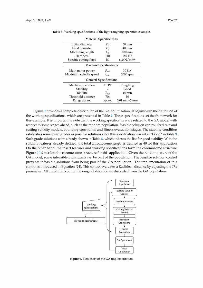
Figure 9 provides a complete description of the GA optimization. It begins with the definition ofthe working specifications, which are presented in Table 9. These specifications set the framework forthis example. It is important to note that the working specifications are related to the GA model withrespect to some stages ahead, such as the random population, feasible solution control, feed rate andcutting velocity models, boundary constraints and fitness evaluation stages. The stability conditionestablishes some insert grades as possible solutions since this specification was set at “Good” in Table 9.Such grade solutions were already shown in Table 8, which indexes the list for good stability. With thestability features already defined, the total chromosome length is defined as 40 for this application.On the other hand, the insert features and working specifications form the chromosome structure.Figure 10 describes the chromosome structure for this application. Given the random nature of theGA model, some infeasible individuals can be part of the population. The feasible solution controlprevents infeasible solutions from being part of the GA population. The implementation of thiscontrol is introduced in Equation (24). This control evaluates a Euclidean distance by adjusting the Thdparameter. All individuals out of the range of distance are discarded from the GA population.Appl. Sci. 2019, 9 FOR 17

Figure 9. Flowchart of the GA implementation.

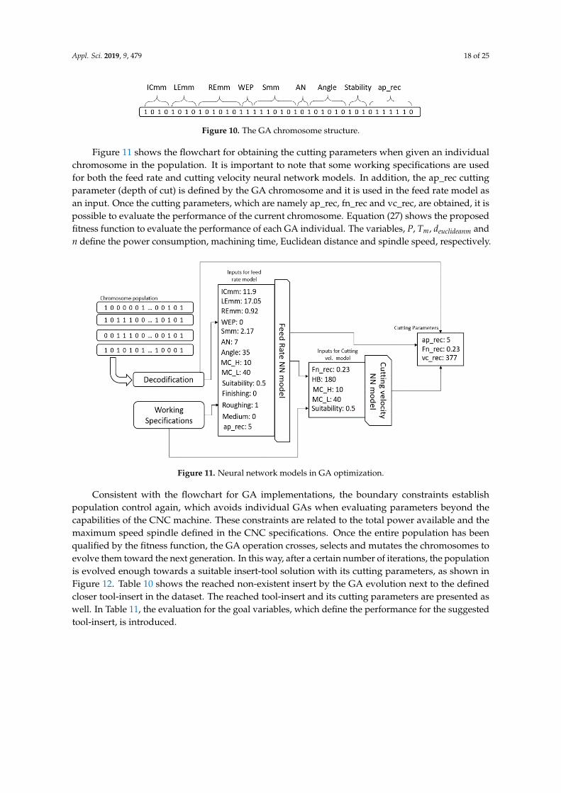
Figure 10. The GA chromosome structure.

Figure 11 shows the flowchart for obtaining the cutting parameters when given an individual

chromosome in the population. It is important to note that some working specifications are used for

both the feed rate and cutting velocity neural network models. In addition, the ap_rec cutting

parameter (depth of cut) is defined by the GA chromosome and it is used in the feed rate model as

an input. Once the cutting parameters, which are namely ap_rec, fn_rec and vc_rec, are obtained, it

is possible to evaluate the performance of the current chromosome. Equation (27) shows the proposed

fitness function to evaluate the performance of each GA individual. The variables, P , mT , euclideanmd

and n define the power consumption, machining time, Euclidean distance and spindle speed,

respectively.

Figure 11. Neural network models in GA optimization.


Appl. Sci. 2019, 9, 479 18 of 25












respectively.

Figure 11. Neural network models in GA optimization.


Figure 11 shows the flowchart for obtaining the cutting parameters when given an individualchromosome in the population. It is important to note that some working specifications are usedfor both the feed rate and cutting velocity neural network models. In addition, the ap_rec cuttingparameter (depth of cut) is defined by the GA chromosome and it is used in the feed rate model asan input. Once the cutting parameters, which are namely ap_rec, fn_rec and vc_rec, are obtained, it ispossible to evaluate the performance of the current chromosome. Equation (27) shows the proposedfitness function to evaluate the performance of each GA individual. The variables, P, Tm, deuclideanm andn define the power consumption, machining time, Euclidean distance and spindle speed, respectively.












respectively.

Figure 11. Neural network models in GA optimization. Figure 11. Neural network models in GA optimization.

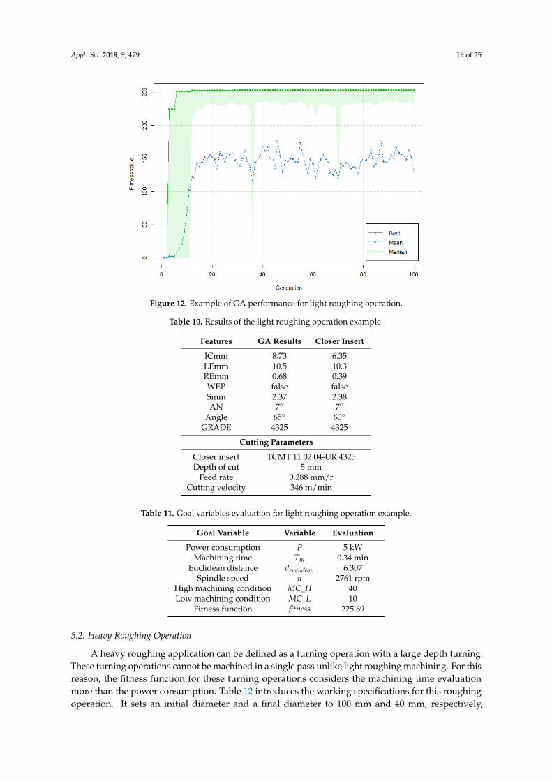
Consistent with the flowchart for GA implementations, the boundary constraints establishpopulation control again, which avoids individual GAs when evaluating parameters beyond thecapabilities of the CNC machine. These constraints are related to the total power available and themaximum speed spindle defined in the CNC specifications. Once the entire population has beenqualified by the fitness function, the GA operation crosses, selects and mutates the chromosomes toevolve them toward the next generation. In this way, after a certain number of iterations, the populationis evolved enough towards a suitable insert-tool solution with its cutting parameters, as shown inFigure 12. Table 10 shows the reached non-existent insert by the GA evolution next to the definedcloser tool-insert in the dataset. The reached tool-insert and its cutting parameters are presented aswell. In Table 11, the evaluation for the goal variables, which define the performance for the suggestedtool-insert, is introduced.

Appl. Sci. 2019, 9, 479 19 of 25


Consistent with the flowchart for GA implementations, the boundary constraints establish

population control again, which avoids individual GAs when evaluating parameters beyond the

capabilities of the CNC machine. These constraints are related to the total power available and the

maximum speed spindle defined in the CNC specifications. Once the entire population has been

qualified by the fitness function, the GA operation crosses, selects and mutates the chromosomes to

evolve them toward the next generation. In this way, after a certain number of iterations, the

population is evolved enough towards a suitable insert-tool solution with its cutting parameters, as

shown in Figure 12. Table 10 shows the reached non-existent insert by the GA evolution next to the

defined closer tool-insert in the dataset. The reached tool-insert and its cutting parameters are

presented as well. In Table 11, the evaluation for the goal variables, which define the performance for

the suggested tool-insert, is introduced.

Figure 12. Example of GA performance for light roughing operation.

Table 10. Results of the light roughing operation example.

Features GA Results Closer Insert

ICmm 8.73 6.35

LEmm 10.5 10.3

REmm 0.68 0.39

WEP false false

Smm 2.37 2.38

AN 7° 7°

Angle 65° 60°

GRADE 4325 4325

Cutting Parameters

Closer insert TCMT 11 02 04-UR 4325

Depth of cut 5 mm

Feed rate 0.288 mm/r

Cutting velocity 346 m/min

Table 11. Goal variables evaluation for light roughing operation example.

Goal Variable Variable Evaluation

Power consumption P 5 kW

Machining time mT 0.34 min

Figure 12. Example of GA performance for light roughing operation.

Table 10. Results of the light roughing operation example.


ICmm 8.73 6.35LEmm 10.5 10.3REmm 0.68 0.39WEP false falseSmm 2.37 2.38AN 7◦ 7◦

Angle 65◦ 60◦

GRADE 4325 4325

Cutting Parameters

Closer insert TCMT 11 02 04-UR 4325Depth of cut 5 mm

Feed rate 0.288 mm/rCutting velocity 346 m/min

Table 11. Goal variables evaluation for light roughing operation example.


Power consumption P 5 kWMachining time Tm 0.34 min

Euclidean distance deuclidean 6.307Spindle speed n 2761 rpm

High machining condition MC_H 40Low machining condition MC_L 10

Fitness function fitness 225.69

5.2. Heavy Roughing Operation

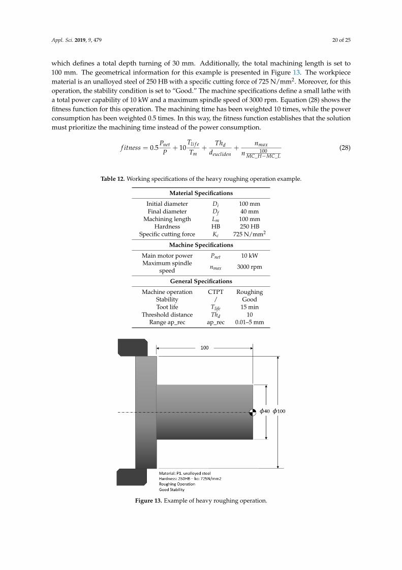
A heavy roughing application can be defined as a turning operation with a large depth turning.These turning operations cannot be machined in a single pass unlike light roughing machining. For thisreason, the fitness function for these turning operations considers the machining time evaluationmore than the power consumption. Table 12 introduces the working specifications for this roughingoperation. It sets an initial diameter and a final diameter to 100 mm and 40 mm, respectively,

Appl. Sci. 2019, 9, 479 20 of 25

which defines a total depth turning of 30 mm. Additionally, the total machining length is set to100 mm. The geometrical information for this example is presented in Figure 13. The workpiecematerial is an unalloyed steel of 250 HB with a specific cutting force of 725 N/mm2. Moreover, for thisoperation, the stability condition is set to “Good.” The machine specifications define a small lathe witha total power capability of 10 kW and a maximum spindle speed of 3000 rpm. Equation (28) shows thefitness function for this operation. The machining time has been weighted 10 times, while the powerconsumption has been weighted 0.5 times. In this way, the fitness function establishes that the solutionmust prioritize the machining time instead of the power consumption.

f itness = 0.5Pnet

P+ 10

Tli f e

Tm+

Thddeucliden

+nmax

n 100MC_H−MC_L

(28)

Table 12. Working specifications of the heavy roughing operation example.


Initial diameter Di 100 mmFinal diameter Df 40 mm

Machining length Lm 100 mmHardness HB 250 HB

Specific cutting force Kc 725 N/mm2


Main motor power Pnet 10 kWMaximum spindle

speed nmax 3000 rpm


Machine operation CTPT RoughingStability / GoodToot life Tlife 15 min

Threshold distance Thd 10Range ap_rec ap_rec 0.01–5 mmAppl. Sci. 2019, 9 FOR 20

Figure 13. Example of heavy roughing operation.

Table 13 shows the results for the GA evolution, which are the obtained features for the GA

algorithm next to the closer tool-insert in the dataset. This table also presents the suggested tool-insert

and its cutting parameters for this operation. Furthermore, in Table 14, the evaluation for the goal

variables, which define the performance for the reached tool-insert, is introduced.

Table 13. Results of the heavy roughing operation example.


ICmm 15.87 12.07

LEmm 21.2 11.7

REmm 0.609 1.19

WEP false false

Smm 5.56 4.76

AN 7° 7°

Angle 90° 90°

GRADE 4325 4325

Cutting Parameters

Closer insert CCMT 12 04 12-PR 4325

Number of passes 6

Depth of cut 5 mm

Feed rate 0.325 mm/r


Table 14. Goal variables evaluation of the heavy roughing operation example.

Goal variable Variable Evaluation

Power consumption P 5.13 kW

Total power consumption Ppasses 30.83 kW

Machining time mT 1.84 min

Euclidean distance euclideand 4.7830

Spindle speed n 2080 rpm

High machining condition HMC _ 40

Low machining condition LMC _ 10


Figure 13. Example of heavy roughing operation.

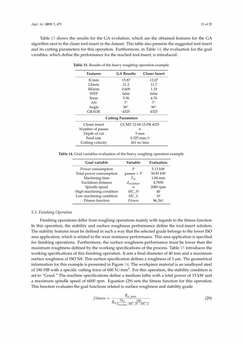
Appl. Sci. 2019, 9, 479 21 of 25

Table 13 shows the results for the GA evolution, which are the obtained features for the GAalgorithm next to the closer tool-insert in the dataset. This table also presents the suggested tool-insertand its cutting parameters for this operation. Furthermore, in Table 14, the evaluation for the goalvariables, which define the performance for the reached tool-insert, is introduced.

Table 13. Results of the heavy roughing operation example.


ICmm 15.87 12.07LEmm 21.2 11.7REmm 0.609 1.19WEP false falseSmm 5.56 4.76AN 7◦ 7◦

Angle 90◦ 90◦

GRADE 4325 4325

Cutting Parameters

Closer insert CCMT 12 04 12-PR 4325Number of passes 6

Depth of cut 5 mmFeed rate 0.325 mm/r


Table 14. Goal variables evaluation of the heavy roughing operation example.

Goal variable Variable Evaluation

Power consumption P 5.13 kWTotal power consumption passes× P 30.83 kW

Machining time Tm 1.84 minEuclidean distance deuclidean 4.7830

Spindle speed n 2080 rpmHigh machining condition MC_H 40Low machining condition MC_L 10

Fitness function Fitness 86.261

5.3. Finishing Operation

Finishing operations differ from roughing operations mainly with regards to the fitness function.In this operation, the stability and surface roughness performance define the tool-insert solution.The stability features must be defined in such a way that the selected grade belongs to the lower ISOarea application, which is related to the wear resistance performance. This area application is specifiedfor finishing operations. Furthermore, the surface roughness performance must be lower than themaximum roughness defined by the working specifications of the process. Table 15 introduces theworking specifications of this finishing operation. It sets a final diameter of 40 mm and a maximumsurface roughness of ISO N8. This surface specification defines a roughness of 3 µm. The geometricalinformation for this example is presented in Figure 14. The workpiece material is an unalloyed steelof 180 HB with a specific cutting force of 600 N/mm2. For this operation, the stability condition isset to “Good.” The machine specifications define a medium lathe with a total power of 15 kW anda maximum spindle speed of 6000 rpm. Equation (29) sets the fitness function for this operation.This function evaluates the goal functions related to surface roughness and stability grade.

f itness =Ra_max

RaThd

deucliden100

MC_H−MC_L

(29)

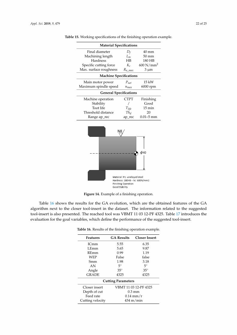
Appl. Sci. 2019, 9, 479 22 of 25

Table 15. Working specifications of the finishing operation example.


Final diameter Df 40 mmMachining length Lm 50 mm

Hardness HB 180 HBSpecific cutting force Kc 600 N/mm2

Max. surface roughness Ra_max 3 µm


Main motor power Pnet 15 kWMaximum spindle speed nmax 6000 rpm


Machine operation CTPT FinishingStability / GoodToot life Tlife 15 min

Threshold distance Thd 20Range ap_rec ap_rec 0.01–5 mm


5.3. Finishing Operation

Finishing operations differ from roughing operations mainly with regards to the fitness function.

In this operation, the stability and surface roughness performance define the tool-insert solution. The

stability features must be defined in such a way that the selected grade belongs to the lower ISO area

application, which is related to the wear resistance performance. This area application is specified for

finishing operations. Furthermore, the surface roughness performance must be lower than the

maximum roughness defined by the working specifications of the process. Table 15 introduces the

working specifications of this finishing operation. It sets a final diameter of 40 mm and a maximum

surface roughness of ISO N8. This surface specification defines a roughness of 3 μm. The geometrical

information for this example is presented in Figure 14. The workpiece material is an unalloyed steel

of 180 HB with a specific cutting force of 600 N/mm2. For this operation, the stability condition is set

to “Good.” The machine specifications define a medium lathe with a total power of 15 kW and a

maximum spindle speed of 6000 rpm. Equation (29) sets the fitness function for this operation. This

function evaluates the goal functions related to surface roughness and stability grade.

L_MCH_MCd

Th

R

Rfitness

eucliden

d

a

max_a

−++=

100 (29)

Table 15. Working specifications of the finishing operation example.


Final diameter fD 40 mm

Machining length mL 50 mm

Hardness HB 180 HB

Specific cutting force cK 600 N/mm2

Max. surface roughness max_aR 3 μm


Main motor power netP 15 kW

Maximum spindle speed maxn 6000 rpm


Machine operation CTPT Finishing

Stability / Good

Toot life lifeT 15 min

Threshold distance dTh 20

Range ap_rec ap_rec 0.01–5 mm

Figure 14. Example of a finishing operation. Figure 14. Example of a finishing operation.

Table 16 shows the results for the GA evolution, which are the obtained features of the GAalgorithm next to the closer tool-insert in the dataset. The information related to the suggestedtool-insert is also presented. The reached tool was VBMT 11 03 12-PF 4325. Table 17 introduces theevaluation for the goal variables, which define the performance of the suggested tool-insert.

Table 16. Results of the finishing operation example.


ICmm 5.55 6.35LEmm 5.65 9.87REmm 0.99 1.19WEP False falseSmm 1.98 3.18AN 5◦ 5◦

Angle 35◦ 35◦

GRADE 4325 4325

Cutting Parameters

Closer insert VBMT 11 03 12-PF 4325Depth of cut 0.3 mm

Feed rate 0.14 mm/rCutting velocity 434 m/min

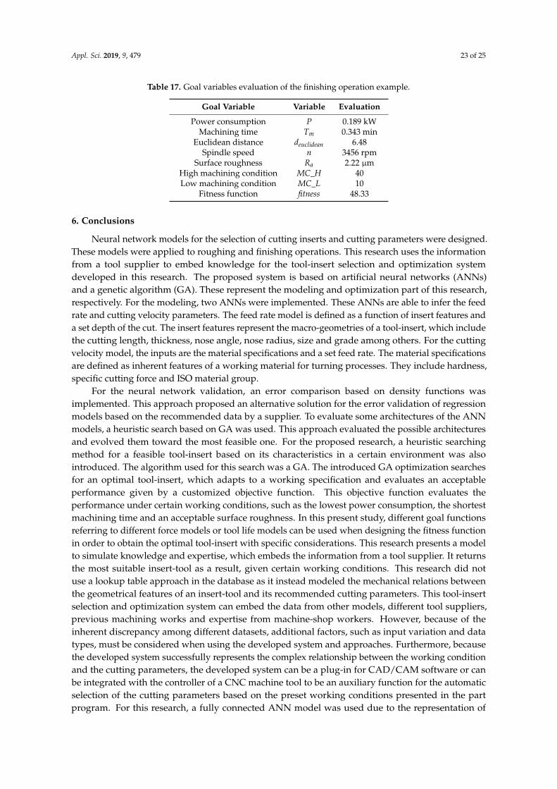
Appl. Sci. 2019, 9, 479 23 of 25

Table 17. Goal variables evaluation of the finishing operation example.


Power consumption P 0.189 kWMachining time Tm 0.343 min

Euclidean distance deuclidean 6.48Spindle speed n 3456 rpm

Surface roughness Ra 2.22 µmHigh machining condition MC_H 40Low machining condition MC_L 10


6. Conclusions

Neural network models for the selection of cutting inserts and cutting parameters were designed.These models were applied to roughing and finishing operations. This research uses the informationfrom a tool supplier to embed knowledge for the tool-insert selection and optimization systemdeveloped in this research. The proposed system is based on artificial neural networks (ANNs)and a genetic algorithm (GA). These represent the modeling and optimization part of this research,respectively. For the modeling, two ANNs were implemented. These ANNs are able to infer the feedrate and cutting velocity parameters. The feed rate model is defined as a function of insert features anda set depth of the cut. The insert features represent the macro-geometries of a tool-insert, which includethe cutting length, thickness, nose angle, nose radius, size and grade among others. For the cuttingvelocity model, the inputs are the material specifications and a set feed rate. The material specificationsare defined as inherent features of a working material for turning processes. They include hardness,specific cutting force and ISO material group.

For the neural network validation, an error comparison based on density functions wasimplemented. This approach proposed an alternative solution for the error validation of regressionmodels based on the recommended data by a supplier. To evaluate some architectures of the ANNmodels, a heuristic search based on GA was used. This approach evaluated the possible architecturesand evolved them toward the most feasible one. For the proposed research, a heuristic searchingmethod for a feasible tool-insert based on its characteristics in a certain environment was alsointroduced. The algorithm used for this search was a GA. The introduced GA optimization searchesfor an optimal tool-insert, which adapts to a working specification and evaluates an acceptableperformance given by a customized objective function. This objective function evaluates theperformance under certain working conditions, such as the lowest power consumption, the shortestmachining time and an acceptable surface roughness. In this present study, different goal functionsreferring to different force models or tool life models can be used when designing the fitness functionin order to obtain the optimal tool-insert with specific considerations. This research presents a modelto simulate knowledge and expertise, which embeds the information from a tool supplier. It returnsthe most suitable insert-tool as a result, given certain working conditions. This research did notuse a lookup table approach in the database as it instead modeled the mechanical relations betweenthe geometrical features of an insert-tool and its recommended cutting parameters. This tool-insertselection and optimization system can embed the data from other models, different tool suppliers,previous machining works and expertise from machine-shop workers. However, because of theinherent discrepancy among different datasets, additional factors, such as input variation and datatypes, must be considered when using the developed system and approaches. Furthermore, becausethe developed system successfully represents the complex relationship between the working conditionand the cutting parameters, the developed system can be a plug-in for CAD/CAM software or canbe integrated with the controller of a CNC machine tool to be an auxiliary function for the automaticselection of the cutting parameters based on the preset working conditions presented in the partprogram. For this research, a fully connected ANN model was used due to the representation of

Appl. Sci. 2019, 9, 479 24 of 25

a multi-dimensional space using the training data obtained from a database. Other networks withdiverse characteristics, such as the convolutional networks, could also be used in future researches.Moreover, methods, such as the support vector machine and probabilistic regression, could be used forregression modeling. This research has used a GA for optimization. However, methods, such as theparticle swarm optimization and gradient descent technique, can also be used to carry out optimization.

Author Contributions: Investigation, B.S.-P., D.H. and S.-S.Y.; Supervision, S.-S.Y.

Funding: This research was funded in part by the Ministry of Science and Technology, Taiwan, R.O.C., underContract MOST104-2221-E-027-132 and MOST103-2218-E-009-027-MY2.

Acknowledgments: The authors would like to thank Hao-Wei Nien (Advantech-LNC Technology Co. Ltd.,Taiwan, R.O.C.) and Chao-Choung Mai (ITRI Intelligent Machinery Technology Center, Taiwan, R.O.C.) fortheir suggestions.

Conflicts of Interest: The authors declare no conflict of interest.

References

1. Weyer, S.; Schmitt, M.; Ohmer, M.; Gorecky, D. Towards industry 4.0—Standardization as the crucialchallenge for highly modular, multi-vendor production systems. IFAC-Pap. 2015, 48, 579–584. [CrossRef]

2. Leo Kumar, S.P. State of the art—Intense review on artificial intelligence systems application in processplanning and manufacturing. Eng. Appl. Artif. Intell. 2017, 65, 294–329. [CrossRef]

3. Zarkti, H.; El Mesbahi, A.; Rechia, A.; Jaider, O. Towards an automatic-Optimized tool selection for millingprocess, based on data from Sandvik Coromant. In Proceedings of the Xème Conférence Internationale:Conception et Production Intégrées, Tanger, Morocco, 3–4 December 2015.

4. Arrazola, P.J.; Özel, T.; Umbrello, D.; Davies, M.; Jawahir, I.S. Recent advances in modelling of metalmachining processes. CIRP Ann. 2013, 62, 695–718. [CrossRef]

5. Ganesh, N.; Kumar, M.U.; Kumar, C.V.; Kumar, B.S. Optimization of cutting parameters in turning of EN 8steel using response surface method and genetic algorithm. Int. J. Mech. Eng. Robot. Res. 2014, 3, 75–86.

6. Yang, Y.; Li, X.; Gao, L.; Shao, X. A new approach for predicting and collaborative evaluating the cuttingforce in face milling based on gene expression programming. J. Netw. Comput. Appl. 2013, 36, 1540–1550.[CrossRef]

7. Cabrera, F.M.; Beamud, E.; Hanafi, I.; Khamlichi, A.; Jabbouri, A. Fuzzy logic-based modeling of surface roughnessparameters for CNC turning of PEEK CF30 by TiN-coated cutting tools. J. Thermoplast. Compos. Mater. 2011, 24,399–413. [CrossRef]

8. Joshi, S.R.; Ganjigatti, J.P. Application of general regression neural networks for forward and reversemodeling of aluminum alloy AA5083; H111 TIG welding process and comparison with feed forward backpropagation, Elman back propagation neural networks. Int. J. Eng. Technol. Sci. Res. 2017, 4, 16–26.

9. Li, H.Z.; Guo, S.; Li, C.J.; Sun, J.Q. A hybrid annual power load forecasting model based on generalizedregression neural network with fruit fly optimization algorithm. Knowl. -Based Syst. 2013, 37, 378–387.[CrossRef]

10. Cairns, J.; McPherson, N.; Galloway, A. Using artificial neural networks to identify and optimise the keyparameters affecting geometry of a GMAW fillet weld. In Proceedings of the 18th International Conferenceon Joining Materials, JOM-18, Helsingor, Denmark, 26–29 April 2015.

11. Arezoo, B.; Ridgway, K.; Al-Ahmari, A.M.A. Selection of cutting tools and conditions of machining operationsusing an expert system. Comput. Ind. 2000, 42, 43–58. [CrossRef]

12. Dereli, T.; Filiz, I.H.; Baykasoglu, A. Optimizing cutting parameters in process planning of prismatic partsby using genetic algorithms. Int. J. Prod. Res. 2001, 39, 3303–3328. [CrossRef]

13. Benkedjouh, T.; Medjaher, K.; Zerhouni, N.; Rechak, S. Health assessment and life prediction of cutting toolsbased on support vector regression. J. Intell. Manuf. 2015, 26, 213–223. [CrossRef]

14. Özel, T.; Hsu, T.K.; Zeren, E. Effects of cutting edge geometry, workpiece hardness, feed rate and cutting speed onsurface roughness and forces in finish turning of hardened AISI H13 steel. Int. J. Adv. Manuf. Technol. 2004, 25,262–269. [CrossRef]

http://dx.doi.org/10.1016/j.ifacol.2015.06.143

http://dx.doi.org/10.1016/j.engappai.2017.08.005

http://dx.doi.org/10.1016/j.cirp.2013.05.006

http://dx.doi.org/10.1016/j.jnca.2013.02.004

http://dx.doi.org/10.1177/0892705710391562

http://dx.doi.org/10.1016/j.knosys.2012.08.015

http://dx.doi.org/10.1016/S0166-3615(99)00051-2

http://dx.doi.org/10.1080/00207540110057891

http://dx.doi.org/10.1007/s10845-013-0774-6

http://dx.doi.org/10.1007/s00170-003-1878-5

Appl. Sci. 2019, 9, 479 25 of 25

15. Xiong, J.; Zhang, G.; Hu, J.; Wu, L. Bead geometry prediction for robotic GMAW-based rapid manufacturingthrough a neural network and a second-order regression analysis. J. Intell. Manuf. 2012, 25, 157–163.[CrossRef]

16. Babu, K.V.; Narayanan, R.G.; Kumar, G.S. An expert system based on artificial neural network for predictingthe tensile behavior of tailor welded blanks. Expert Syst. Appl. 2009, 36, 10683–10695. [CrossRef]

17. Özel, T.; Karpat, Y. Predictive modeling of surface roughness and tool wear in hard turning using regressionand neural networks. Int. J. Mach. Tools Manuf. 2005, 45, 467–479. [CrossRef]

18. Malinov, S.; Sha, W.; McKeown, J.J. Modelling the correlation between processing parameters and propertiesin titanium alloys using artificial neural network. Comput. Mater. Sci. 2001, 21, 375–394. [CrossRef]

19. Kuo, R.J.; Chen, C.H.; Hwang, Y.C. An intelligent stock trading decision support system through integrationof genetic algorithm based fuzzy neural network and artificial neural network. Fuzzy Sets Syst. 2001, 118,21–45. [CrossRef]

20. Quiza Sardiñas, R.; Rivas Santana, M.; Alfonso Brindis, E. Genetic algorithm-based multi-objectiveoptimization of cutting parameters in turning processes. Eng. Appl. Artif. Intell. 2006, 19, 127–133.[CrossRef]

21. Cus, F.; Balic, J. Optimization of cutting process by GA approach. Robot. Comput. -Integr. Manuf. 2003, 19,113–121. [CrossRef]

22. Suresh, P.V.S.; Rao, P.V.; Deshmukh, S.G. A genetic algorithmic approach for optimization of surfaceroughness prediction model. Int. J. Mach. Tools Manuf. 2002, 42, 675–680. [CrossRef]

23. Yang, W.H.; Tarng, Y.S. Design optimization of cutting parameters for turning operations based on theTaguchi method. J. Mater. Process. Technol. 1998, 84, 122–129. [CrossRef]

24. Thamizhmanii, S.; Saparudin, S.; Hasan, S. Analyses of surface roughness by turning process using Taguchimethod. J. Achiev. Mater. Manuf. Eng. 2007, 20, 503–506.

25. Sandvik Coromant. Available online: https://www.sandvik.coromant.com/en-gb/pages/default.aspx(accessed on 9 October 2017).

26. Murata, N.; Yoshizawa, S.; Amari, S. Network information criterion-determining the number of hidden unitsfor an artificial neural network model. IEEE Trans. Neural Netw. 1994, 5, 865–872. [CrossRef] [PubMed]

27. Arnaiz-González, Á.; Fernández-Valdivielso, A.; Bustillo, A.; López de Lacalle, L.N. Using artificial neuralnetworks for the prediction of dimensional error on inclined surfaces manufactured by ball-end milling.Int. J. Adv. Manuf. Technol. 2016, 83, 847–859. [CrossRef]

28. Jain, S.P.; Ravindra, H.V.; Ugrasen, G.; Prakash, G.V.N.; Rammohan, Y.S. Study of surface roughness and AEsignals while machining titanium grade-2 material using ANN in WEDM. In Materials Today: Proceedings;Elsevier: Amsterdam, The Netherlands, 2017; pp. 9557–9560.

29. Anastasiadis, A.D.; Magoulas, G.D.; Vrahatis, M.N. New globally convergent training scheme based on theresilient propagation algorithm. Neurocomputing 2005, 64, 253–270. [CrossRef]

30. Twomey, J.M.; Smith, A.E. Validation and verification. In Artificial Neural Networks for Civil Engineers:Fundamentals and Applications; Expert Systems and Artificial Intelligence Committee, Ed.; American Societyof Civil Engineers: Reston, VA, USA, 1997; pp. 44–64.

31. Olden, J.D.; Jackson, D.A. Illuminating the “black box”: A randomization approach for understandingvariable contributions in artificial neural networks. Ecol. Model. 2002, 154, 135–150. [CrossRef]

32. Bishop, C.M. Pattern Recognition and Machine Learning; Springer: New York, NY, USA, 2011.33. Scrucca, L. GA: A package for genetic algorithms in R. J. Stat. Softw. 2013, 53, 1–37. [CrossRef]

© 2019 by the authors. Licensee MDPI, Basel, Switzerland. This article is an open accessarticle distributed under the terms and conditions of the Creative Commons Attribution(CC BY) license (http://creativecommons.org/licenses/by/4.0/).

http://dx.doi.org/10.1007/s10845-012-0682-1

http://dx.doi.org/10.1016/j.eswa.2009.02.044

http://dx.doi.org/10.1016/j.ijmachtools.2004.09.007

http://dx.doi.org/10.1016/S0927-0256(01)00160-4

http://dx.doi.org/10.1016/S0165-0114(98)00399-6

http://dx.doi.org/10.1016/j.engappai.2005.06.007

http://dx.doi.org/10.1016/S0736-5845(02)00068-6

http://dx.doi.org/10.1016/S0890-6955(02)00005-6

http://dx.doi.org/10.1016/S0924-0136(98)00079-X

https://www.sandvik.coromant.com/en-gb/pages/default.aspx

http://dx.doi.org/10.1109/72.329683

http://www.ncbi.nlm.nih.gov/pubmed/18267861

http://dx.doi.org/10.1007/s00170-015-7543-y

http://dx.doi.org/10.1016/j.neucom.2004.11.016

http://dx.doi.org/10.1016/S0304-3800(02)00064-9

http://dx.doi.org/10.18637/jss.v053.i04

http://creativecommons.org/

http://creativecommons.org/licenses/by/4.0/.

Cutting Insert and Parameter Optimization for Turning Based ...

Documents