Customer Concentration and Cost Structure Hsihui Chang KPMG Professor of Accounting LeBow College of Business Drexel University Philadelphia, PA 19104 Curtis M. Hall Assistant Professor LeBow College of Business Drexel University Philadelphia, PA 19104 Michael T. Paz PhD Candidate LeBow College of Business Drexel University Philadelphia, PA 19104 May, 2014

Welcome message from author
This document is posted to help you gain knowledge. Please leave a comment to let me know what you think about it! Share it to your friends and learn new things together.
Transcript

Customer Concentration and Cost Structure
Hsihui Chang KPMG Professor of Accounting
LeBow College of Business Drexel University
Philadelphia, PA 19104
Curtis M. Hall Assistant Professor
LeBow College of Business Drexel University
Philadelphia, PA 19104
Michael T. Paz PhD Candidate
LeBow College of Business Drexel University
Philadelphia, PA 19104
May, 2014
Customer Concentration and Cost Structure
Abstract
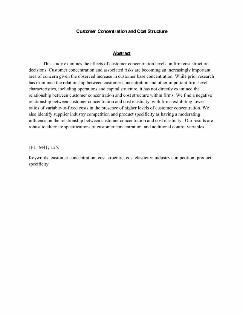
This study examines the effects of customer concentration levels on firm cost structure decisions. Customer concentration and associated risks are becoming an increasingly important area of concern given the observed increase in customer base concentration. While prior research has examined the relationship between customer concentration and other important firm-level characteristics, including operations and capital structure, it has not directly examined the relationship between customer concentration and cost structure within firms. We find a negative relationship between customer concentration and cost elasticity, with firms exhibiting lower ratios of variable-to-fixed costs in the presence of higher levels of customer concentration. We also identify supplier industry competition and product specificity as having a moderating influence on the relationship between customer concentration and cost elasticity. Our results are robust to alternate specifications of customer concentration and additional control variables.
JEL: M41; L25.
Keywords: customer concentration; cost structure; cost elasticity; industry competition; product specificity.

1
I . INTRODUCTION
This paper examines the impact of customer concentration on firm cost structure
decisions, which are among the most important strategic decisions made by managers (Banker et
al. 2014). The
only impacts firm operations, but also its ability to realize profit from those operations. More
rigid cost structures (i.e. cost structures that include a higher proportion of fixed costs to variable
costs) generally lead to higher contribution margins relative to more flexible cost structures,
thereby allowing firms to generate higher levels of profit when sales are strong. Cost structure
can also be difficult to change in the short-run, particularly when it contains a high proportion of
fixed costs, due to the difficulties involved in eliminating committed resources. It is therefore not
surprising that cost structure decisions incorporate a variety of operating and environmental
factors, including economic, regulatory, and production considerations. Despite the fact that
both academics and practitioners have highlighted customer-base concentration as a critical
environmental consideration for firms, prior literature has not considered the potential
relationship between customer concentration and firm cost structure.
Customer concentration and relationships with major customers have become an
increasingly important area of interest for both researchers and practitioners as customer bases
become more concentrated (Patatoukas 2012). The manufacturing sector, in particular, has seen
significant increases in customer concentration over the past few decades (Kelly and Gosman
2000). Aside from its financial performance implications, customer concentration also
influences firm-level decisions related to capital structure and operations. For example, the
presence of major customers can impact firm-level decisions related to the breadth and depth of
its product offerings (Ketokivi and Jokinen 2006). Prior literature on the firm-level effects of
2
customer concentration provides conflicting predictions as to its potential impact on firm cost
structure. Economic dependencies which arise between a supplier and their major customers
grow as those customers contribute a higher proportion of firm revenues. This economic
dependence creates significant financial risks for the supplier. By contrast, firms may also derive
operating benefits from their relationships with major customers as a result of mutually
beneficial cooperation. These conflicting effects of customer concentration on the internal
operating environments of firms make it difficult to predict its effect on firm cost structure.
While recent literature has examined the impact of other environmental factors on firm cost
structure decisions, it remains an open empirical question as to how customer concentration
influences such decisions within firms. Thus, it is important to understand the relationship
between customer concentration and firm cost structure within the manufacturing sector.
To address our research question we use cost data from a sample of U.S. manufacturing
firms between the years 1976 through 2013. Following Kallapur and Eldenburg (2005) and
Banker et al. (2014), we specify a log-linear model to examine changes in firm cost structure.
We employ a measure of customer concentration used in prior literature (Patatoukas 2012) to
examine the impact of customer concentration on firm cost elasticity. This measure provides
by calculating the
proportion of total sales revenue contributed by each major customer and summing those
proportions. Our empirical results demonstrate a negative association between customer
concentration and cost elasticity among suppliers within the manufacturing sector, with suppliers
increasing their proportion of fixed-to-variable costs as their customer base becomes more
concentrated. Furthermore, we examine the moderating influence of supplier industry
competition and product specificity and find that both exacerbate the impact of customer
3
concentration on supplier cost elasticity. Our results are robust to alternate specifications of
customer concentration and the inclusion of controls for demand uncertainty, leverage, and asset
and employee intensity.
Our study makes several contributions to the literature. We contribute to the literature on
cost behavior by identifying customer concentration as a determinant of firm cost structure.
This finding may help reconcile conflicting results from prior research related to cost behavior.
Our identification of supplier industry competition and product specificity as moderators of the
relationship between customer concentration and firm cost structure also highlights the
importance of considering interactions between internal and external environmental factors
which influence firm operations. Furthermore, our results add to the growing body of literature
on the impact of customer concentration and major customers on firms by examining how firms
adjust their operations in response to risks and opportunities arising from customer base
concentration.
The rest of the paper is organized as follows: Section II provides an overview of relevant
literature and develops hypotheses related to our research questions. Section III includes a
description of our sample, related descriptive statistics, and our estimation models. Section IV
presents and discusses our empirical results, after which Section V provides our concluding
remarks.
I I . LITERATURE REVIEW AND HYPOTHESIS DEVELOPMENT
Customer Concentration
customer
exhibit a higher level of customer concentration (Patatoukas 2012). The Statement of Financial

4
Accounting Standards (SFAS) 131 (FASB 1997) requires that firms disclose the presence of any
and all customers which contribute 10% of enterprise-wide revenue, either to a single segment or
across multiple segments. T
reflects the traditional view that customer concentration presents significant risks for firms.
Scherer (1970) and Gosman and Kohlbeck (2009) suggest that a customer power increases in
their level of contribution to firm sales revenue. As customer power grows, suppliers face
mounting incentives to retain the business of major customers and, consequently, reduced
bargaining power.
Reductions in supplier bargaining power resulting from customer concentration have
been shown to have a negative impact on operational performance. Lustgarten (1975) finds that
reduced supplier power results in a negative relationship between customer concentration and
profit margins. Galbrath and Stiles (1983) similarly find that more concentrated customer bases
are associated with lower operating profit margins related to downward price pressure from
customers. Gosman and Kohlbeck (2009) document negative relationships between the presence
of major customers and both gross margins and return on assets (ROA). These negative
profitability effects reflect increased levels of idiosyncratic risk associated with the potential
adverse demand, sales growth, stock market, and default risk impacts of losing a major customer
(Albuquerque et al. 2010). Balakrishan et al. (1996) similarly find that firms with higher levels of
customer concentration experience greater declines in ROA in response to adopting Just-in-Time
(JIT) production methods. Customer concentration is also positively related to bankruptcy risk
(Becchetti and Sierra 2003) and the probability of receiving a going concern opinion (Dhaliwal
et al. 2013) stemming from the potential for major customer defection. Cohen and Frazzini
(2008) find that relationships between suppliers and their strong customers create economic
5
dependence between the two firms such that economic shocks to one firm lead to a reciprocal
shock in the other. This economic dependence arises in part from relationship-specific
investments with limited transferability and liquidity (Raman & Shahrur 2008). Bae and Wang
(2010) also find that firms with major customers face increased distress costs upon entering
bankruptcy , resulting in such firms maintaining higher cash levels to stave off the liquidation of
relationship-specific investments in the event of financial distress.
Despite the aforementioned negative effects, customer concentration has also been
shown to accrue benefits to suppliers. Gosman & Kohlbeck (2009) find that major customers are
associated with improved inventory and payables management among suppliers. Lilien (1983)
finds that firms with higher levels of customer concentration spend less money on marketing and
trade show participation. More generally, Patatoukas (2012) find that firms with major customers
benefit from lower sales, general, and administrative (SG&A) costs, higher ROA, and higher
return on equity (ROE). Matsumura and Schloetzer (2012) also document increased asset
turnover in the presence of major customers which they suggest reflects improvements in
demand forecasting and inventory management arising from cooperation between suppliers and
their major customers. A number of other studies support their view that higher levels of
coordination and information sharing between suppliers and their major customers can benefit
suppliers. Kulp et al. (2004) observe increased supplier margins associated supplier-customer
cooperation on inventory replenishment and improved performance associated with supplier-
customer cooperation on product/service development. Additionally, information sharing on
inventory and product needs generally improves both supplier profitability and customer
inventory management, suggesting the existence of financial incentives for supplier-customer
cooperation. Schloetzer (2012) finds additional incentives for customers to cooperate with
6
suppliers through process integration and sharing in the form of improved financial performance
associated with such cooperation. Wasti & Liker (1997), using survey data from a group of
Japanese automotive component suppliers, finds that supplier-customer cooperation on product
design benefits the supplier through improved design for manufacturability and the customer
through enhanced conformity between supplier designs and customer product feature demands.
Prior literature suggests conflicting predictions related to the impact of customer
concentration on firm cost structure. Higher levels of customer concentration are associated with
significant financial and operational risks arising from the potential for losing a major customer.
These risks present significant forecasting and planning difficulties which may prompt firms to
use real options and more elastic (i.e. flexible) cost structures as a hedge against default. On the
other hand, cooperation and demand stability associated with strong customer-supplier
relationships likely improves the ability of suppliers to forecast and plan for future production
requirements. Additionally, major customer relationships may necessitate relationship-specific
investments in order to fulfill customer production requirements. While we expect to observe a
relationship between customer concentration and firm cost structure, the aforementioned
operational impacts of customer concentration do not allow us to predict the direction of this
relationship. Therefore, we hypothesize:
H1: Customer concentration will be related to supplier cost elasticity
The Impact of Supplier Industry Competition
Differences in the level of supplier industry competition may have a moderating
influence on the relationship between customer concentration and firm cost structure. Snyder
(1998) developed an analytical model which examines the impact of customer size on supplier
competition. Their model demonstrates that larger buyers are able to obtain lower overall prices

7
on their purchases due to supplier competition for their business. As the incentives to gain or
ease, such customers bargaining power also increases.
Becker and Thomas (2008) demonstrate this phenomenon empirically by identifying spillover
effects between changes in customer industry concentration and subsequent supplier industry
concentration. They attribute this effect to the positive relationship between customer industry
concentration (i.e. customer size) and customer bargaining power. Subsequent changes in
supplier industry concentration are, therefore, explainable attempts to offset changes in customer
bargaining power associated with industry consolidation. Brown et al. (2009) find that investors
understand and trade on this increased risk, resulting in negative abnormal returns for suppliers
whose customers are involved in a leveraged buyout. This evidence suggests that higher levels
of customer concentration signal the presence of larger customers which may attract direct
competition from rival suppliers. As supplier industry competition increases, the prospect that a
supplier may have to
1998). Simultaneously, suppliers in highly competitive industries seek out new customers in an
effort to stimulate firm growth, increase market share, and generate positive returns for investors.
Customer concentration, therefore, likely heightens the uncertainty created by high levels of
industry competition.
Prior literature provides conflicting evidence related to the impact of industry
highly competitive product markets undertake lower levels of current irreversible capital
investments, including fixed asset purchases, when price uncertainty increases. This suggests
. Recent work by
Banker et al. (2014), however, suggests that the introduction of additional demand uncertainty
8
stimulated by industry competition should result in lower levels of cost elasticity as firms guard
against the potential for demand spikes. Customer concentration likely intensifies the effects of
industry competition on cost elasticity, since customer concentration signals the presence of
attractive customers which must be defended from rival suppliers. Since we expect the industry
competition to moderate the relationship between customer concentration and cost elasticity, we
specify the following hypothesis:
H2: Supplier industry competition levels have a moderating effect on the relationship between customer concentration and supplier cost elasticity
The Impact of Product Specificity
Given that prior literature has demonstrated a negative relationship between the breadth
of supplier product offerings and customer concentration (Ketokivi and Jokinen 2006), we also
examine the potential moderating influence of product specificity on the relationship between
customer concentration and firm cost structure. Customer-specific and unique products arise as a
result of information sharing and product design collaboration between suppliers and their major
customers (Anderson & Decker 2009; Wasti & Liker 1997). While supplier-customer product
design cooperation increases the likelihood that customers will be satisfied with the final product
(and, thus, more likely to purchase), producing unique and/or specialized products requires
costly investments in R&D (Titman & Wessels 1998). Such relationship-specific investments in
assets and product design are generally associated with long-term customer relationships and
product differentiation strategies (Ketokivi & Jokinen 2006). Suppliers undertaking such
relationship-spending, however, tend to benefit from increased barriers to entry as a result of
high levels of product specificity which reduce substitutability (Winter & Szulanski 2001).
It is unclear what impact product specificity will have on the relationship between
customer concentration and supplier cost structure. Investments in relationship-specific assets
9
associated with higher levels of customer concentration have been shown to increase transaction
risk (Dekker et al. 2013), economic dependence (Patatoukas 2012), hold-up problems (Grossman
& Hart 1986), earnings volatility and earnings management (Raman & Shahrur 2008), distress
costs associated with bankruptcy, and opportunity costs associated with increased cash holdings
(Bae & Wang 2010). Additionally, losing a major customer represents the potential to seriously
erode the value of any relationship-specific investments (Dhaliwal et al. 2013). Each of these
effects suggests that product specificity creates uncertainty which will lead to lower levels of
fixed costs within a supplier cost structure. Anderson and Decker (2009), however, point out
that relationship-specific investments can increase the cost of switching suppliers and effectively
deter major customers from switching to new suppliers. Kumar (1996) also points out that
relationship-specific investments reflect the presence of trust between suppliers and their major
customers. This trust is realized in the form of greater cooperation and supply chain
coordination (Joshi & Stump 1999), extended trade credit terms provided to customers during
periods of liquidity shock (Cuñat 2007), and greater overall supply-chain stability and efficiency
through trade credit provision (Yang & Birge 2013). These factors suggest that product
specificity reduces uncertainty, potentially leading to higher levels of fixed costs within a
supplier s cost structure. Accordingly, we hypothesize the following:
H3: Product specificity levels have a moderating effect on the relationship between customer concentration and supplier cost elasticity
I I I . DATA AND METHODOLOGY
Sample
We build our sample beginning with major customer information reported in the
Compustat Segment Files following the methodology proposed by Patatoukas (2012). Major
customer data disclosed in the annual reports of manufacturing firms (SIC Codes 20 39)
10
between 1976 and 2013 is gathered from the Compustat Segment Files, including customer
name, type, and revenue contributed to the supplier firm. This customer information is then
matched to the corresponding supplier data from the Compustat Annual File using gvkey codes.
In order to match customers and supplier with different fiscal year end dates, we use the most
recent customer information available as of the month of the -end date. Our
final matched supplier-customer sample consists of all firms reporting at least one major
customer during the sample period.
After compiling our matched supplier-customer sample, we gather additional supplier
financial information related to operating costs and sales revenue. Following Banker et al.
(2014), we focus on three categories of costs: SG&A costs, COGS, and the number of
employees. Additionally, we gather information on a fourth category of costs: total operating
costs. We discard all observations for which either current or lagged sales or total operating costs
are missing. We are left with a final sample of 46,836 firm-year observations across the entire
sample period. Table 1 reports a description of the sample composition by industry.
Observations from firms in the electronic equipment and components industry,
industrial/commercial machinery and computer equipment industry, and chemicals and allied
products industry make up slightly more than 50% of the sample.
< Insert Table 1 About Here >
Descriptive Statistics
Table 2 presents descriptive statistics for our variables of interest. Differences in
numbers of observations across variables are attributable to missing data. While we excluded
observations which did not have total operating cost data, for example, we did not exclude
observations which were missing any of the three sub-categories of operating costs (SG&A,

11
COGS, or # of Employees). Our descriptive statistics are reported in CPI adjusted dollars
deflated using 1982-1984 as the base year. The average (median) firm in our sample reported
sales revenue of $753 ($51) million dollars and total operating costs of $675 ($50) million. As
shown in Table 1, observations with values of log-changes in revenue, total operating costs,
SG&A costs, COGS, or number of employees in the highest and lowest 0.5% of the distribution
are truncated in order to control for the potential influence of outliers on our results.
< Insert Table 2 About Here >
We construct our customer concentration variable (CC) using major customer data
disclosed by firms under the provisions of SFAS 131 (FASB 1997). We adopt a measure
developed by Patatoukas (2012) which uses a modification of the Herfindahl-Hirschman index to
capture both the total number of majo
of firm customer-
base concentration (CC) in year t, essentially a weighted-average index of customer-specific
revenue to total firm revenue, is described by the equation
(1)
where Salesijt represents firm i sales to customer j in year t and Salesit represents total sales for
firm i in year t. Average (median) customer concentration is 0.1333 (0.0622) for our sample of
firms. We also report results using an alternate specification of our customer concentration
This
threshold has been used in prior literature as a proxy for customer concentration (Bae & Wang
2010; Gosman & Kohlbeck 2009; Gosman et al. 2004). 74.84% of firms in our sample report at
least one customer who contributes 10% or more of overall firm revenues.
Model Specification
12
Following a methodology proposed in prior research (Kallapur and Eldenburg 2005;
Banker et al. 2014), we examine our research questions using a log-linear cost function which
regresses log-transformed changes in costs on concurrent log-transformed changes in sales
revenues. Accordingly, we specify the following log-linear cost function for estimation
0 1 2 3GDP (Rev) 4Size 5 6GDPGrowth 7Size (2) 1-19 1-19
where the term is the log-transformed change in costs for a firm between year t-1 and
year t. We estimate Equation (2) using four separate specifications of the term: total
operating costs (OC), selling, general, and administrative costs (SGA), number of employees
(EMP), and cost of goods sold (COGS). The term is specified as the log-transformed
change in revenue for a firm between year t-1 and year t. RankCC refers to a ranked
transformation of the customer concentration measure. We construct the variable RankCC by
first calculating the value for our customer concentration measure as described in Equation (1)
for each firm-year observation. We then rank each firm into deciles based on their customer
concentration score. RankCC is defined as the decile rank of a firm for year t. Size is defined as
the natural log of sales for a firm in year t. GDPGrowth refers to the log-transformed change in
Gross Domestic Product between year t-1 and year t. We include controls for GDP growth (log
change in GDP) and firm size (natural log of sales) as well as interactions between each variable
and log-changes in revenue. Following the procedure described by Peterson (2009), we cluster
by firm standard errors by firm when conducting our analysis. Our model also includes controls
for industry fixed effects (IndFE) and interactions between our industry indicators and log-
changes in revenue . Additionally, we control for the potential impact of
13
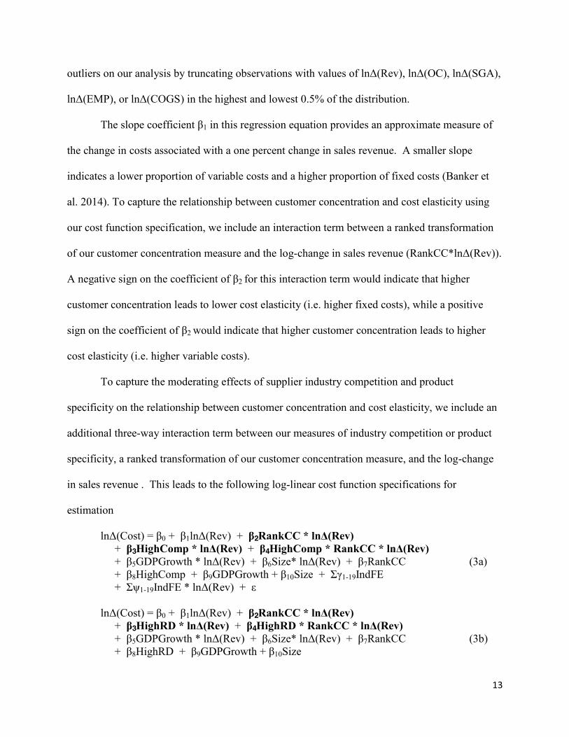
outliers on our analysis by truncating observations with values of Rev), OC) ),
) ) in the highest and lowest 0.5% of the distribution.
The slope coefficient 1 in this regression equation provides an approximate measure of
the change in costs associated with a one percent change in sales revenue. A smaller slope
indicates a lower proportion of variable costs and a higher proportion of fixed costs (Banker et
al. 2014). To capture the relationship between customer concentration and cost elasticity using
our cost function specification, we include an interaction term between a ranked transformation
of our customer concentration measure and the log-change in sales revenue (RankCC* ).
A negative sign on the coefficient of 2 for this interaction term would indicate that higher
customer concentration leads to lower cost elasticity (i.e. higher fixed costs), while a positive
sign on the coefficient of 2 would indicate that higher customer concentration leads to higher
cost elasticity (i.e. higher variable costs).
To capture the moderating effects of supplier industry competition and product
specificity on the relationship between customer concentration and cost elasticity, we include an
additional three-way interaction term between our measures of industry competition or product
specificity, a ranked transformation of our customer concentration measure, and the log-change
in sales revenue . This leads to the following log-linear cost function specifications for
estimation
0 1 2 + 3 + 4 + 5 6Size + 7RankCC (3a) + 8HighComp + 9GDPGrowth 10Size + 1-19IndFE + 1-19
0 1 2 + 3 + 4 + 5 6Size + 7RankCC (3b) 8HighRD + 9GDPGrowth 10Size

14
+ 1-19IndFE + 1-19
where the terms HighComp and HighRD are both indicator variables which indicate the
presence of high levels of competition and research and development (R&D) intensity,
respectively, within a firm We construct the variable HighComp which is included in
Equation (3a) by first estimating -Hirschman Index (HHI) using their
three-digit SIC code as a proxy for supplier industry competition (Ellis et al 2012). We then set
the indicator variable HighCo
median and zero otherwise. Similarly, we calculate the variable HighRD which is included in
Equation (3b) by first estimating R&D intensity as the ratio of R&D expense to sales. We adopt
this measure as a proxy for product specificity following the methodology used by Raman and
Shahrur (2008)
intensity is above the industry median and zero otherwise. All other variable definitions are the
same as those described earlier for Equation (2). We summarize our variable definitions in
Appendix A. Note that while we estimate equations (3a) and (3b) for all four specifications of
the term used in estimating Equation (2), we report only those results for total
operating costs (OC) for the purpose of brevity.
IV. EMPIRICAL RESULTS
Correlation Analysis
Table 3 reports correlations among the variables used in our multivariate tests. Spearman
(Pearson) correlations are reported in the upper (lower) diagonal. We observe a negative and
statistically significant correlation between firm -.167, p < .01) and
Rank -.164, p < .01), results which provide preliminary evidence suggesting that
customer bases are more concentrated among smaller firms. We also observe a positive and
15
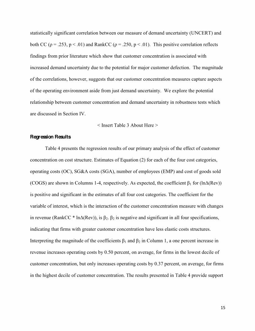
statistically significant correlation between our measure of demand uncertainty (UNCERT) and
= .253, p < .01) and Rank
findings from prior literature which show that customer concentration is associated with
increased demand uncertainty due to the potential for major customer defection. The magnitude
of the correlations, however, suggests that our customer concentration measures capture aspects
of the operating environment aside from just demand uncertainty. We explore the potential
relationship between customer concentration and demand uncertainty in robustness tests which
are discussed in Section IV.
< Insert Table 3 About Here >
Regression Results
Table 4 presents the regression results of our primary analysis of the effect of customer
concentration on cost structure. Estimates of Equation (2) for each of the four cost categories,
operating costs (OC), SG&A costs (SGA), number of employees (EMP) and cost of goods sold
(COGS) are shown in Columns 1-4, respectively. As expected, the coefficient 1 for ( )
is positive and significant in the estimates of all four cost categories. The coefficient for the
variable of interest, which is the interaction of the customer concentration measure with changes
in revenue ( ) 2. 2 is negative and significant in all four specifications,
indicating that firms with greater customer concentration have less elastic costs structures.
Interpreting the magnitude of the coefficients 1 2 in Column 1, a one percent increase in
revenue increases operating costs by 0.50 percent, on average, for firms in the lowest decile of
customer concentration, but only increases operating costs by 0.37 percent, on average, for firms
in the highest decile of customer concentration. The results presented in Table 4 provide support

16
for H1 and are consistent with firms choosing greater fixed costs compared to variable costs
when they have more concentrated customer bases.
< Insert Table 4 About Here >
Next we examine the effects of industry competition and product specificity on the
relationship between customer concentration and cost structure. The regression results are
presented in Table 5.1 Column 1 presents estimates for Equation (3a) which examines the effects
of industry competition. The coefficient 4 is for the variable of interest, which is specified as the
three-way interaction of a high competition indicator variable with the customer concentration
measure and changes in revenue (HighComp * )). Additionally we add the
interaction of high competition with changes in revenue to control for the main effect of supplier
industry competition on cost structure as HighComp * ). As we can observe from
Column 1 of Table 5, the coefficients on 3 and 4 are both negative and statistically significant,
providing support for H2. This is consistent with supplier industry competition intensifying the
effect of customer concentration on cost elasticity. On average, a one percent increase in revenue
increases operating costs by 0.42 percent (0.51 - 0.09) for firms with high customer
concentration compared to an increase of 0.30 percent (0.51 - 0.09 -0.06 -0.06) for high customer
concentration firms operating under high competition.
< Insert Table 5 About Here >
Column 2 of Table 5 presents estimates for Equation (3b) which examines the effect of
product specificity on the relationship between customer concentration and cost structure. The
main effect of product specificity on cost structure is captured by 3, the interaction of a high
R&D intensity indicator variable with changes in revenue (HighRD * )). The
1 For brevity, we present only estimates of operation costs in Table 5, but estimates for the other three cost categories lead to the same interpretation. Additionally, operating costs include all of the other three cost categories (SGA, COGS and employee costs).

17
incremental effect of product specificity on the relationship between customer concentration and
cost structure is measured 4 , the three-way interaction term HighRD * ).
As shown in Column 2 of the same table, the coefficients on 3 4 are both negative and
statistically significant, providing support for H3. This result suggests that fixed-to-variable cost
ratios will be higher for firms with higher levels of customer concentration when product
specificity is also high compared to when product specificity is lower.
Additional Analysis and Robustness Checks
To evaluate the robustness of our primary results, we perform the following additional
analysis. First, we include an additional control for the effect of leverage on firm cost structure
decisions. Prior studies have shown that customer concentration is also related to capital
structure decisions. Banerjee et al. (2008) provide evidence that firms with major customers tend
to hold less debt, though Hennessy and Livdan (2009) also find that firms increase in response to
increases in the bargaining power of their business partners. Higher levels of leverage can
potentially affect cost structure by increasing the risk of bankruptcy, which may incentivize
managers to choose more elastic cost structures (Novy-Mark 2011). However, many firms will
use debt financing to pay for fixed assets and relationship-specific investments, both of which
would decrease cost elasticity. We control for the effect of leverage using the indicator variable
HighDebt. We construct the variable HighDebt by first calculating the debt-to-equity ratio for
each firm-year observation. We then set HighDebt equal to one for firm-year observations
which are above the sample median and zero otherwise. Table 6 presents results after controlling
for leverage. In Column 1, we present estimates for a re-specification of Equation (2) which
includes an additional interaction between the HighDebt variable and changes in revenue
(HighDebt )). Columns 2 and 3 present subsample analysis results for Equation (2)
18
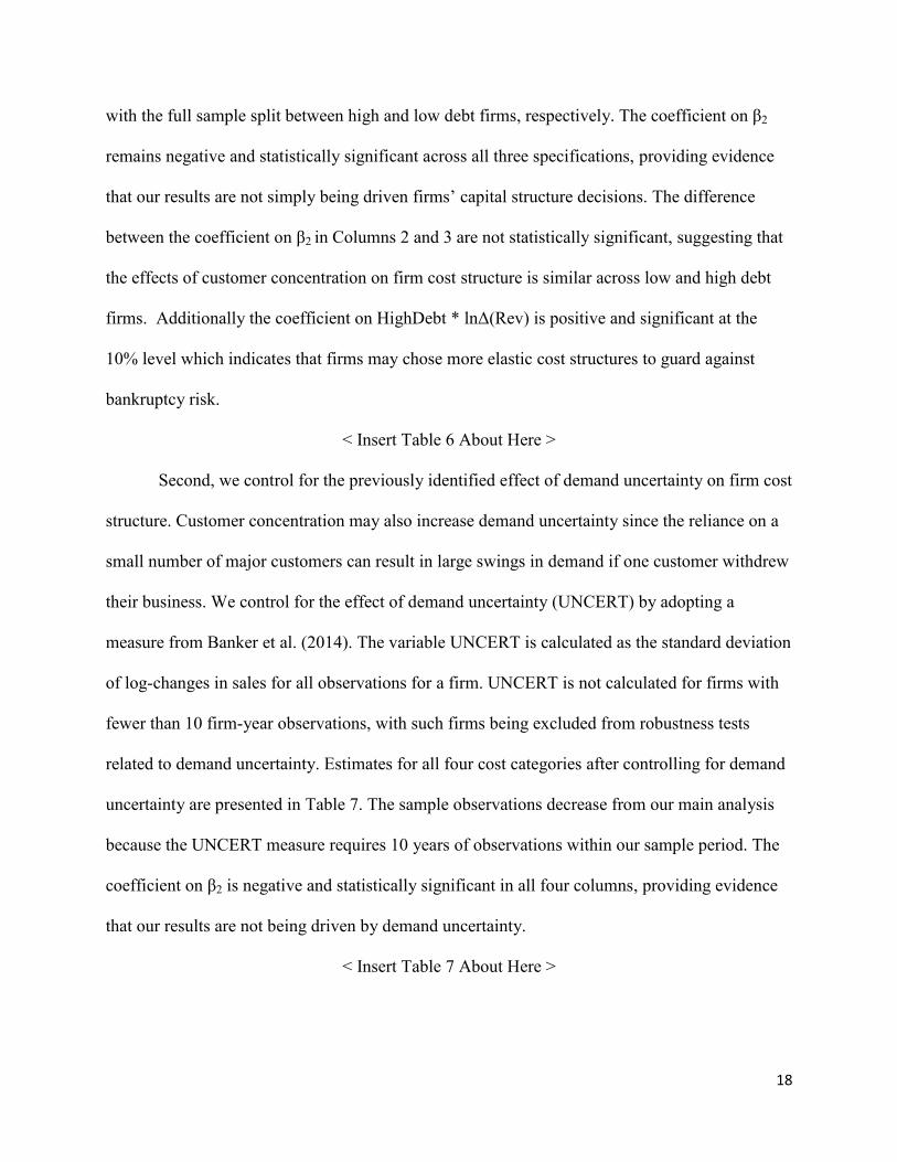
with the full sample split between high and low debt firms, respectively 2
remains negative and statistically significant across all three specifications, providing evidence
The difference
between 2 in Columns 2 and 3 are not statistically significant, suggesting that
the effects of customer concentration on firm cost structure is similar across low and high debt
firms. Additionally the coefficient on HighDebt ) is positive and significant at the
10% level which indicates that firms may chose more elastic cost structures to guard against
bankruptcy risk.
< Insert Table 6 About Here >
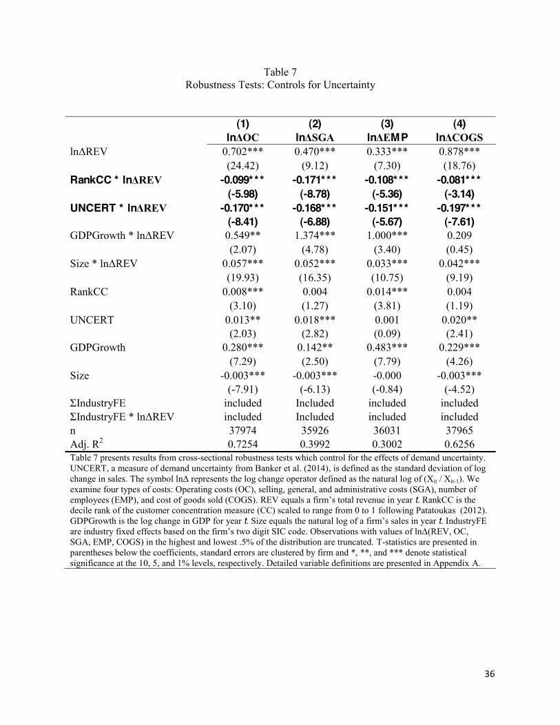
Second, we control for the previously identified effect of demand uncertainty on firm cost
structure. Customer concentration may also increase demand uncertainty since the reliance on a
small number of major customers can result in large swings in demand if one customer withdrew
their business. We control for the effect of demand uncertainty (UNCERT) by adopting a
measure from Banker et al. (2014). The variable UNCERT is calculated as the standard deviation
of log-changes in sales for all observations for a firm. UNCERT is not calculated for firms with
fewer than 10 firm-year observations, with such firms being excluded from robustness tests
related to demand uncertainty. Estimates for all four cost categories after controlling for demand
uncertainty are presented in Table 7. The sample observations decrease from our main analysis
because the UNCERT measure requires 10 years of observations within our sample period. The
2 is negative and statistically significant in all four columns, providing evidence
that our results are not being driven by demand uncertainty.
< Insert Table 7 About Here >
19
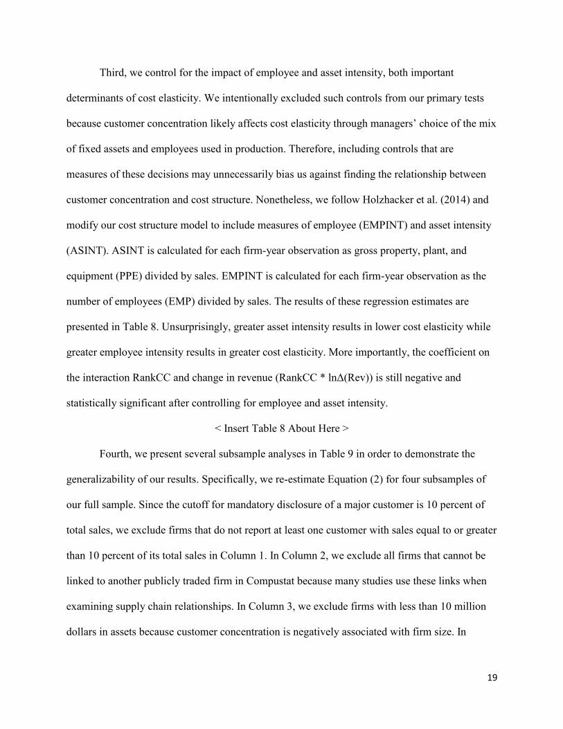
Third, we control for the impact of employee and asset intensity, both important
determinants of cost elasticity. We intentionally excluded such controls from our primary tests
of fixed assets and employees used in production. Therefore, including controls that are
measures of these decisions may unnecessarily bias us against finding the relationship between
customer concentration and cost structure. Nonetheless, we follow Holzhacker et al. (2014) and
modify our cost structure model to include measures of employee (EMPINT) and asset intensity
(ASINT). ASINT is calculated for each firm-year observation as gross property, plant, and
equipment (PPE) divided by sales. EMPINT is calculated for each firm-year observation as the
number of employees (EMP) divided by sales. The results of these regression estimates are
presented in Table 8. Unsurprisingly, greater asset intensity results in lower cost elasticity while
greater employee intensity results in greater cost elasticity. More importantly, the coefficient on
the interaction RankCC and change in revenue ( ) is still negative and
statistically significant after controlling for employee and asset intensity.
< Insert Table 8 About Here >
Fourth, we present several subsample analyses in Table 9 in order to demonstrate the
generalizability of our results. Specifically, we re-estimate Equation (2) for four subsamples of
our full sample. Since the cutoff for mandatory disclosure of a major customer is 10 percent of
total sales, we exclude firms that do not report at least one customer with sales equal to or greater
than 10 percent of its total sales in Column 1. In Column 2, we exclude all firms that cannot be
linked to another publicly traded firm in Compustat because many studies use these links when
examining supply chain relationships. In Column 3, we exclude firms with less than 10 million
dollars in assets because customer concentration is negatively associated with firm size. In

20
Column 4, we examine the subsample of observations after the passage of SFAS 131 in 1997.
The coefficient on 2 is negative and statistically significant across all four subsamples. In
untabulated results, we also measure customer concentration using the raw CC score from
Patatoukas (2012) and using an indicator variable for whether the firm has at least one customer
which accounts for more than 10 percent of its sales. Our results are qualitatively unchanged
when using these measures.
< Insert Table 9 About Here >
Fifth, we investigate potential multicollinearity in our analysis by calculating variable
inflation factors (VIFs) for all regressions reported in Tables 4 through 9. Greene (2008)
suggests a VIF cutoff value of 10 as indicating a high level of multicollinearity. In untabulated
results, VIFs are below 10 for all variables except for in our reported results, suggesting
that multicollinearity is not a significant problem for the majority of variables in our analysis.
The high VIF value for ) is expected given that it is used to form interaction terms in all
of our models. Brambor et al. (2006) suggest that the potential for making inferential errors due
to the exclusion of formative terms in models which include multiplicative interaction terms
outweighs any potential benefits from excluding such terms. Consequently, we continue to
include the term in our analysis.
Finally, we re-estimate our regression models using two alternative methods of dealing
with outlying observations to ensure that our results are robust. First, we winsorize (rather than
truncate) observations with values of Rev), OC) ) (EMP) )
in the highest and lowest 0.5% of the distribution. Second, we re-estimate our regression models
without truncating or winsorizing outlying observations. Results using these methods of dealing
21
with outlying observations yield the same inferences as the results reported in Tables 4 through
9.
V. CONCLUSIONS
We examine the relationship between customer concentration and cost elasticity within
firms. Analyzing cost data for a sample of U.S. manufacturing firms for the period 1976-2013,
we find a negative relationship between customer concentration and cost elasticity, with firms
exhibiting lower proportions of variable-to-fixed costs in the presence of more concentrated
customer bases. This negative relationship is strengthened by the presence of significant supplier
market concentration and product specificity.
Additional analysis shows that these results hold after controlling for the effects of
demand uncertainty, supplier leverage, and both asset and employee sensitivity. Our results are
robust to alternative specifications of customer concentration. We attribute this relationship both
to supplier investments in relationship-specific assets and improved cost efficiency in the
presence of higher levels of customer concentration. These results support findings from prior
literature which suggest that suppliers derive material benefits from their relationships with
major customers.
Our study contributes to the literature by highlighting the importance of considering
customers when examining firm cost structure. Our study also informs results from prior
research related to demand uncertainty and cost structure by highlighting the impact of cross-
sectional differences in customer concentration across industries. Our identification of two
significant moderators of the relationship between customer concentration and firm cost
structure, supplier market competition and product specificity, highlights the need for academics
and practitioners to consider how internal and external operating environment characteristics

22
interact to influence firm-level decisions. Finally, our results add to the growing body of
literature on the impact of customer concentration and major customers on firms by examining
how firms adjust their operations in response to risks and opportunities arising from customer
base concentration.
23
REFERENCES
Albuquerque, A., G. Papadakis, and P. Wysocki, 2010. The Impact of Risk and Monitoring on
CEO Compensation. Working paper, Boston University and University of Miami.
Anderson, S. W., and H. C. Dekker. 2009. Strategic cost management in supply chains part 1:
Structural cost management. Accounting Horizons 23(2): 201-220.
Bae, K., and J. Wang. 2010. Why do firms in customer-supplier relationships hold more cash?
Working paper, York University.
Balakrishnan, R., T. J. Linsmeier, and M. Venkatachalam. 1996. Financial benefits from JIT
adoption: Effects of customer concentration and cost structure. The Accounting Review
71(2): 183-205.
Banerjee, S., S. Dasgupta, and Y. Kim. 2008. Buyer-supplier relationships and the stakeholder
theory of capital structure. Journal of Finance 63(5): 2507-2552.
Banker, R. D., D. Byzalov, and J. M. Plehn-Dujowich. 2014. Demand uncertainty and cost
behavior. The Accounting Review (forthcoming)
Becchetti, L., and J. Sierra. 2003. Bankruptcy risk and productive efficiency in manufacturing
firms. Journal of Banking and Finance 27(11): 2099-2120.
Becker, M. J., and S. Thomas. The Spillover Effects of Changes in Industry Concentration.
Working Paper, University of Pittsburgh.
Brambor, T., W. R. Clark, and M. Golder. 2006. Understanding interaction models: Improving
empirical analyses. Political Analysis 14(1): 63-82.
Brown, D. T., C. E. Fee, and S. E. Thomas. 2009. Financial leverage and bargaining power with
suppliers: Evidence from leveraged buyouts. Journal of Corporate Finance 15 (2): 196
211.

24
Cohen, L., and A. Frazzini. 2008. Economic links and predictable returns. Journal of Finance 63
(4): 1977 2011.
Cuñat, V. 2007. Trade credit: Suppliers as debt collectors and insurance providers. The Review of
Financial Studies 20(2): 491-527.
Dekker. H. C., J. Sakaguchi, and T. Kawai. 2013. Beyond the contract: Managing risk in supply
chain relations. Management Accounting Research 24(2): 122-139.
Dhaliwal, D. S., P. N. Michas, V. Naiker, and D. Sharma. 2013. Major Customer Reliance and
Auditor Going-Concern Decisions. Working Paper, University of Arizona, Monash
University, and Kennesaw State University.
Ellis, J. A., C. E. Fee, and S. E. Thomas. 2012. Proprietary costs and the disclosure of
information about customers. Journal of Accounting Research 50(3): 685-728.
Financial Accounting Standards Board (FASB). 1997. Disclosures about Segments of an
Enterprise and Related Information. Statement of Financial Accounting Standards No.
131. Norwalk, CT: FASB.
Ghosal, V., and P. Loungani. 1996. Product market competition and the impact of price
uncertainty on investment: Some evidence from US manufacturing industries. The
Journal of Industrial Economics 44(2): 217-228.
Gosman, M., T. Kelly, P. Olsson, and T. Warfield. 2004. The profitability and pricing of major
customers. Review of Accounting Studies 9 (1): 117 139.
Gosman, M. L., and M. J. Kohlbeck. 2009. Effects of the existence and identity of major
customers on supplier profitability: Is Wal-Mart different? Journal of Management
Accounting Research 21: 179-201.
Greene, W. 2008. Econometric Analysis. Upper Saddle River, NJ: Pearson/Prentice Hall.

25
Grossman, S. J., and O. D. Hart. 1986. The costs and benefits of ownership: A theory of vertical
and lateral integration. Journal of Political Economy 94(4): 691-719.
Hennessy, C. A., and D. Livdan. 2009. Debt, bargaining, and credibility in firm-supplier
relationships. Journal of Financial Economics 93(3): 382-399.
Holzhacker, M., R. Krishnan, and M. D. Mahlendorf. 2014. The impact of changes in regulation
on cost behavior. Contemporary Accounting Research (forthcoming)
Joshi, A. W., and R. L. Stump. 1999. The contingent effect of specific asset investment on joint
action in manufacturer-supplier relationships: An empirical test of the moderating role of
reciprocal asset investments, uncertainty, and trust. Journal of the Academy of Marketing
Science 27(3): 291-305.
Kallapur, S., and L. Eldenburg. 2005. Uncertainty, real options, and cost behavior: evidence
from Washington State hospitals. Journal of Accounting Research 43 (5): 735-752.
Kelly, T., and M. Gosman. 2000. Increased buyer concentration and its effects on profitability in
the manufacturing sector. Review of Industrial Organization 17 (1): 41 59.
Ketokivi, M., and M. Jokinen. 2006. Strategy, uncertainty, and the focused factor in international
process manufacturing. Journal of Operations Management 24(3): 250-270.
Kulp, S. C., H. L. Lee, and E. Ofek. 2004. Manufacturer benefits from information integration
with retail customers. Management Science 50(4): 431-444.
Kumar, N. 1996. The power of trust in manufacturer-retailer relationships. Harvard Business
Review 74 (November): 92 106.
Lilien, G. L. 1983. A descriptive model of the trade-show budgeting decision process. Industrial
Marketing Management 12(1): 25-29.
26
Lustgarten, S. H. 1975. The impact of buyer concentration in manufacturing industries. The
Review of Economics and Statistics 57(2): 125-132.
Matsumura, E. L., and J. D. Schloetzer. 2012. The Cost of Customer and Supplier Financial
Strength Perspectives: Evidence from the Apparel Industry. Working Paper, University of
Wisconsin Madison and Georgetown University.
Novy-Marx, R. 2011. Operating leverage. Review of Finance 15(1): 103-134.
Patatoukas, P. N. 2012. Customer-base concentration: Implications for firm performance and
capital markets. The Accounting Review 87(2): 363-392.
Peterson, M. A. 2009. Estimating standard errors in finance panel data sets: Comparing
approaches. Review of Financial Studies 22(1): 435-480.
Raman, K., and H. Shahrur. 2008. Relationship-specific investments and earnings management:
Evidence on corporate suppliers and customers. The Accounting Review 83(4): 1041-
1081.
Scherer, F. M. 1970. Industrial Market Structure and Economic Performance. Chicago, IL: Rand
McNally.
Schloetzer, J. D. 2012. Process integration and information sharing in supply chains. The
Accounting Review 87(3): 1005-1032.
Snyder, C. M. 1998. Why do larger buyers pay lower prices? Intense supplier competition.
Economics Letters 58(2): 205-209.
Titman, S., and R. Wessels. 1988. The determinants of capital structure choice. Journal of
Finance 43(1): 1-19.
Wasti, S. N., and J. K. Liker. 1997. Risky business or competitive power? Supplier involvement
in Japanese product design. Journal of Product Innovation Management 14(5): 337-355.

27
Winter, S. G., and G. Szulanski. 2001. Replication as strategy. Organization Science 12(6): 730-
743.
Yang, S. A., and J. R. Birge. 2013. How Inventory Is (Should Be) Financed: Trade Credit in
Supply Chains with Demand Uncertainty and Costs of Financial Distress. Working
Paper, London Business School and The University of Chicago.
28
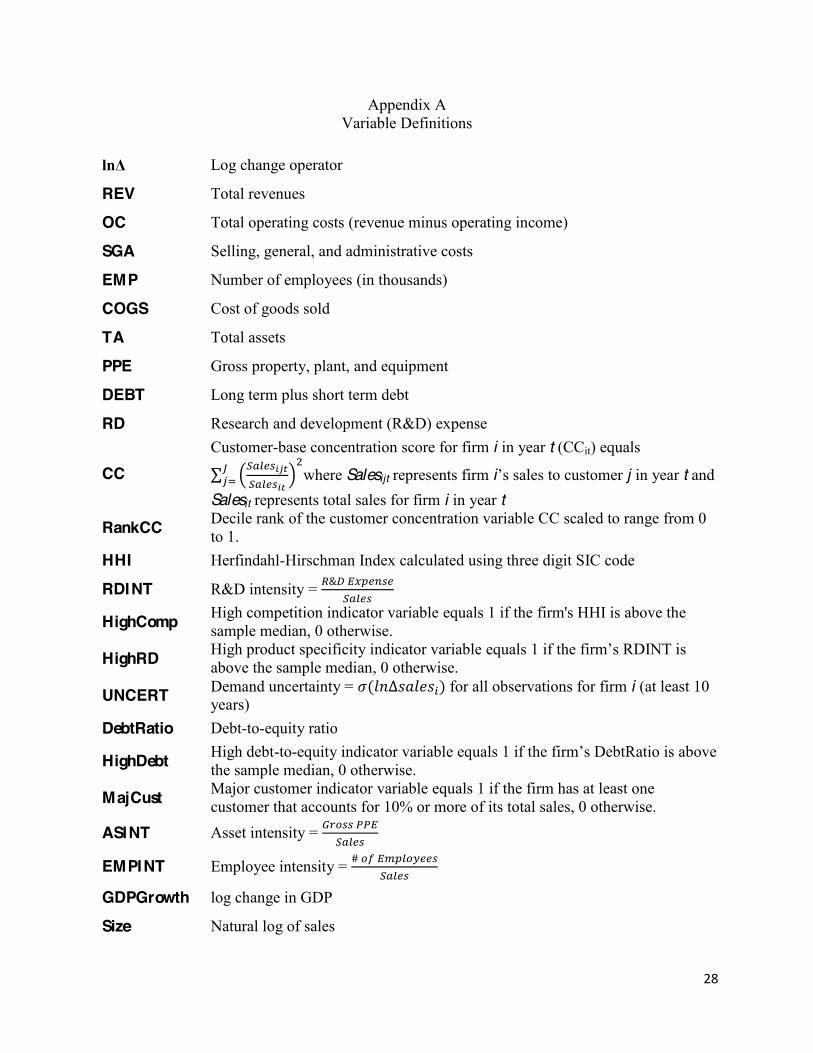
Appendix A Variable Definitions
Log change operator
REV Total revenues
OC Total operating costs (revenue minus operating income)
SGA Selling, general, and administrative costs
EMP Number of employees (in thousands)
COGS Cost of goods sold
TA Total assets
PPE Gross property, plant, and equipment
DEBT Long term plus short term debt
RD Research and development (R&D) expense
CC Customer-base concentration score for firm i in year t (CCit) equals
where Salesijt represents firm i sales to customer j in year t and Salesit represents total sales for firm i in year t
RankCC Decile rank of the customer concentration variable CC scaled to range from 0 to 1.
HHI Herfindahl-Hirschman Index calculated using three digit SIC code
RDINT R&D intensity =
HighComp High competition indicator variable equals 1 if the firm's HHI is above the sample median, 0 otherwise.
HighRD High product specificity indicator variable equals RDINT is above the sample median, 0 otherwise.
UNCERT Demand uncertainty = for all observations for firm i (at least 10 years)
DebtRatio Debt-to-equity ratio
HighDebt High debt-to-equity indicator variable equals 1 if the is above the sample median, 0 otherwise.
MajCust Major customer indicator variable equals 1 if the firm has at least one customer that accounts for 10% or more of its total sales, 0 otherwise.
ASINT Asset intensity =
EMPINT Employee intensity =
GDPGrowth log change in GDP
Size Natural log of sales
29
Table 1 Sample Composition by Industry
2-Digit
SIC Code
Industry Name N % of Sample
20 Food and Kindred Products 2027 4.33% 21 Tobacco Products 101 0.22% 22 Textile Mill Products 755 1.61%
23 Apparel and Other Finished Products Made from Fabrics and Similar Materials 1234 2.63%
24 Lumber and Wood Products, Except Furniture 404 0.86% 25 Furniture and Fixtures 616 1.32% 26 Paper and Allied Products 819 1.75% 27 Printing, Publishing, and Allied Industries 871 1.86% 28 Chemicals and Allied Products 6794 14.51% 29 Petroleum Refining and Related Industries 449 0.96% 30 Rubber and Miscellaneous Plastic Products 1433 3.06% 31 Leather and Leather Products 369 0.79% 32 Stone, Clay, Glass, and Concrete Products 509 1.09% 33 Primary Metal Industries 1587 3.39%
34 Fabricated Metal Products, Except Machinery & Transportation Equipment 1929 4.12%
35 Industrial and Commercial Machinery and Computer Equipment 7075 15.11%
36 Electronic and Other Electrical Equipment and Components, Except Computer Equipment 9600 20.50%
37 Transportation Equipment 2547 5.44%
38 Measuring, Analyzing, and Controlling Instruments; Photographic, Medical, and Optical Goods; Watches and Clocks 6573 14.03%
39 Miscellaneous Manufacturing Industries 1144 2.44%
Total 46836 100.00%
Table 1 presents the industry composition for the sample of firm-year observations used in this study. The sample consists of manufacturing firms (SIC 2000 - 3999) that report at least one strong customer in the Compustat Customer Segment database.
30
Table 2 Descriptive Statistics (CPI adjusted, 1982-1984 base year)
Percentiles
Variable n Mean Std. Dev. 25th 50th 75th REV 46,836 753 3,785 11 51 254 OC 46,836 675 3,432 13 50 233 SGA 44,301 145 684 4 13 50 EMP 45,309 6 22 0 1 3 COGS 46,836 502 2,824 7 33 164 TA 46,836 841 4,813 12 49 237 PPE 46,759 475 3,155 4 18 104 DEBT 46,836 223 1,796 1 5 52 RD 34,446 42 217 1 3 12 CC 46,836 0.1333 0.1812 0.0189 0.0622 0.1721 HHI 46836 0.1723 0.1535 0.0743 0.1209 0.2149 RDINT 46836 0.4621 6.9614 0.0000 0.0256 0.1140 DebtRatio 46835 0.6495 27.8205 0.0119 0.2683 0.7566 UNCERT 37,974 0.3243 0.2931 0.1545 0.2363 0.3772 ASINT 46759 0.6758 2.8530 0.2268 0.3869 0.6450 EMPINT 45309 1.0730 6.8139 0.4121 0.6976 1.1795 MajCust 46,836 0.7484 0.4339 0.0000 1.0000 1.0000 Table 2 presents descriptive statistics for the sample used in the study. REV year t. OC t. SGA equals selling and general costs in year t number of employees (in thousands) in year t. COGS is cost of goods sold in year t gross property plant and equipment in year t short term plus long term debt for year t. RD is research and development (R&D) expense in year t. CC is the measure of customer concentration following Patatoukas (2012) for year t. HHI is Herfindahl-Hirschman Index for year t . RDINT is intensity for year t. DebtRatio is debt to equity ratio for year t. UNCERT is the measure of demand uncertainty from Banker et al. (2014) for year t. ASINT is asset intensity for year t. EMPINT is a
employee intensity for year t. MajCust equals 1 if a firm has at least one customer that accounts for 10% or more of its total sales, 0 otherwise. in the highest and lowest .5% of the distribution are truncated. Detailed variable definitions are presented in Appendix A.
31
Table 3 Correlations
Variable Name 1 2 3 4 5 6 7 8 9 10 11 12 13 14 15 16 17 18
1.REV .990** .929** .936** .979** -.167** -.164** -.094** 1.00** .123** -.103** -.145** -.097** .260** .196** -.482** .039** -.406**
2. OC .995** .942** .931** .985** -.144** -.142** -.103** .990** .093** -.079** -.204** -.067** .253** .194** -.447** .078** -.389**
3.SGA .728** .698** .849** .885** -.125** -.123** -.126** .930** -.022** .023** .040** .081** .146** .145** -.360** .082** -.411**
4. EMP .758** .748** .701** .934** -.196** -.193** -.043** .936** .196** -.181** -.268** -.094** .310** .216** -.523** .121** -.090**
5. COGS .973** .985** .565** .697** -.145** -.143** -.086** .979** .138** -.118** -.278** -.116* .282** .206** -.469** .079** -.352**
6. CC -.017** -.016** -.010 -.040** -.014** .995** -.085** -.167** -.157** .134** .177** .089** -.126** -.070** .253** .041** -.043**
7. RankCC -.018** -.018** -.000 -.047** -.018** .786** -.084** -.164** -.156** .133** .175** .089** -.125** -.069** .250** .041** -.044**
8. GDPGrowth -.060** -.059** -.072** -.036** -.051** -.056** -.072** -.094** .030** -.021** -.022** -.012* .031** -.006 -.000** -.023** .185**
9. Size .391** .381** .427** .497** .342** -.180** -.160** -.086** .123** -.103** -.245** -.097** .260** .196** -.482** .039** -.406**
10. HHI .012** .013** -.011* .052** .019** -.076** -.084** -.017** .097** -.866** -.436** -.174** .208** .073** -.295** -.078** .153**
11. HighComp .000 -.001 .021** -.059** -.007 .115** .133** -.015** -.103** -.631** .380** .152** -.191** -.064** .258** .056** -.174**
12. RDINT -.015** -.014** -.014** -.021** -.013** .147** .079** .003 -.136** -.056** .072** .673** -.295** -.141** .373** .074** -.011*
13. HIGHRD .043** .041** .066** .052** .033** .087** .089** -.011** -.083** -.123** .152** .093** -.163** -.162** .215** .093** .020**
14. DebtRatio .001 .000 -.000 .002 .001 -.007 -.008 .009 .001 -.004 .001 -.001 -.002 .788** -.199** .100** .052**
15. HighDebt ..072** .073** .092** .094** .062** -.079** -.070** -.004 .207** .049** -.064** -.038** -.162** .064** -.118** .077** -.017**
16. UNCERT -.094** -.091** -.106** -.144** -.081** .309** .236** -.018** -.410** -.171** .226** .209** .219** -.002 -.116** -.028** .023**
17. ASINT -.000 -.000 .014** -.005 .000 .124** .065** -.005 -.105** -.037** .053** .520** .061** .000 -.003 .149** .191**
18. EMPINT -.043** -.042** -.102** -.027** -.037** .110** .044** .041** -.213** -.001 -.020** .540** .042** .001 -.029** .150* .740**
**,* indicate statistical significance at the 1 and 5 percent levels, respectively. Significance levels are two-tailed for all variables. Spearman correlations are reported above the diagonal and Pearson correlations are reported below the diagonal.

32
Table 4 Main Results
(1) (2) (3) (4)
ln ln ln MP ln ln 0.507*** 0.285*** 0.157*** 0.744***
(17.88) (7.25) (4.09) (20.28) RankCC * ln -0.138*** -0.209*** -0.133*** -0.092***
(-9.43) (-11.55) (-7.08) (-4.03) GDPGrowth * ln 1.136*** 1.807*** 1.332*** 0.348
(4.57) (5.99) (4.69) (0.86) Size * ln 0.075*** 0.068*** 0.049*** 0.054***
(32.91) (24.39) (18.66) (14.84) RankCC 0.013*** 0.012*** 0.018*** 0.007**
(5.40) (3.48) (4.84) (2.07) GDPGrowth 0.387*** 0.214*** 0.591*** 0.301***
(9.68) (3.69) (9.60) (5.71) Size -0.005*** -0.005*** -0.000 -0.004***
(-11.71) (-9.13) (-0.13) (-6.74) included included included included
ln included included included included n 46836 44086 43580 46819 Adj. R2 0.6929 0.3718 0.2761 0.6076 Table 4 presents results from the following regression:
0 1 2 3GDPGrowth 4Size 5 6GDPGrowth 7Size 1-19 1-19 The term the log change operator defined as the natural log of (Xit / Xit-1). We examine four types of costs: Operating costs (OC), selling, general, and administrative costs (SGA), number of employees (EMP), and cost of goods sold (COGS). REV t. RankCC is the decile rank of the customer concentration measure (CC) scaled to range from 0 to 1 following Patatoukas (2012). GDPGrowth is the log change in GDP for year t. Size equals the natural log of sales in year t. IndustryFE are industry fixed effects based on COGS) in the highest and lowest .5% of the distribution are truncated. T-statistics are presented in parentheses below the coefficients. Standard errors are clustered by firm. *, **, and *** denote statistical significance at the 10, 5, and 1% levels, respectively. Detailed variable definitions are presented in Appendix A.

33
Table 5 Cross-sectional Results for Supplier Industry Competition and Product Specificity
(1) (2)
ln ln
0.509*** 0.529***
(18.52) (16.64)
RankCC * ln -0.092*** -0.059***
(-4.64) (-3.12)
HighComp * ln -0.063***
(-3.88)
HighComp * RankCC * ln -0.058**
(-2.30)
HighRD * ln
-0.133***
(-8.58)
HighRD * RankCC * ln
-0.085***
(-3.54)
GDPGrowth * ln 1.139*** 1.272***
(4.64) (5.34)
Size * ln 0.077*** 0.071***
(34.19) (32.38)
RankCC 0.012*** 0.010***
(5.03) (4.21)
Highcomp 0.005***
(3.06)
HighRD
0.031***
(20.13)
GDPGrowth 0.374*** 0.372***
(9.50) (9.65)
Size -0.005*** -0.005***
(-11.78) (-12.68)
included included ln included included
N 46836 46836 Adj. R2 0.6964 0.7057 Table 5 presents results from cross-sectional tests of the effects of competition and product specificity on the relationship between customer concentration and cost structure. HighComp, our measure of competition, is an indicator variable equal to 1 if the firm's Herfindahl-Hirschman Index (based on three-digit SIC code) is above the sample median and 0 otherwise. HighRD, our measure of product specificity, is an indicator variable equal
the log change operator defined as the natural log of (Xit / Xit-1). We examine four types of costs: Operating costs (OC), selling, general, and administrative costs (SGA), number of employees (EMP), and cost of goods sold (COGS). For brevity, only estimates for operating costs are presented. REV t. RankCC is the decile rank of the customer concentration measure (CC) scaled to range from 0 to 1 following

34
Patatoukas (2012). GDPGrowth is the log change in GDP for year t. Size equals the natural log of sales in year t. IndustryFE are industry fixed effects based on two digit SIC code. Observations with values
REV, OC, SGA, EMP, COGS) in the highest and lowest .5% of the distribution are truncated. T-statistics are presented in parentheses below the coefficients, standard errors are clustered by firm and *, **, and *** denote statistical significance at the 10, 5, and 1% levels, respectively. Detailed variable definitions are presented in Appendix A.
35
Table 6 Robustness Tests: Controls for Debt
(1) (2) (3)
ln ln ln
(Full Sample) (Low Debt) (High Debt) 0.498*** 0.519*** 0.488***
(16.99) (14.47) (12.64) RankCC * ln -0.136*** -0.122*** -0.153***
(-9.29) (-6.28) (-7.11) HighDebt * ln 0.015* (1.75) GDPGrowth * ln 1.139*** 0.939*** 1.376***
(4.57) (2.77) (3.78) Size * ln 0.075*** 0.073*** 0.076***
(32.16) (25.28) (22.01) RankCC 0.013*** 0.009** 0.017***
(5.34) (2.40) (5.58) HighDebt -0.013 (-0.51) GDPGrowth 0.387*** 0.566*** 0.203***
(9.69) (8.68) (4.47) Size -0.005*** -0.004*** -0.006***
(-11.49) (-4.88) (-12.31) included included included
ln included included included N 46836 23242 23594 Adj. R2 0.6930 0.6501 0.7469 Table 6 presents results from cross-sectional and partitioned robustness tests which control for the effects of firm debt. Equation (1) is a cross-sectional analysis which controls for firm debt using an indicator variable. Equations (2) and (3) partition the full sample into low and high debt firms. HighDebt is an indicator variable equal to debt ratio is above the sample median and 0 otherwise. change operator defined as the natural log of (Xit / Xit-1). We examine four types of costs: Operating costs (OC), selling, general, and administrative costs (SGA), number of employees (EMP), and cost of goods sold (COGS).
t. RankCC is the decile rank of the customer concentration measure (CC) scaled to range from 0 to 1 following Patatoukas (2012). GDPGrowth is the log change in GDP for year t. Size equals the natural log of sales in year t. IndustryFE are industry fixed effects based on
.5% of the distribution are truncated. T-statistics are presented in parentheses below the coefficients, standard errors are clustered by firm and *, **, and *** denote statistical significance at the 10, 5, and 1% levels, respectively. Detailed variable definitions are presented in Appendix A.
36
Table 7 Robustness Tests: Controls for Uncertainty
(1) (2) (3) (4)
ln ln ln MP ln ln 0.702*** 0.470*** 0.333*** 0.878***
(24.42) (9.12) (7.30) (18.76) RankCC * ln -0.099*** -0.171*** -0.108*** -0.081***
(-5.98) (-8.78) (-5.36) (-3.14) UNCERT * ln -0.170*** -0.168*** -0.151*** -0.197***
(-8.41) (-6.88) (-5.67) (-7.61) GDPGrowth * ln 0.549** 1.374*** 1.000*** 0.209
(2.07) (4.78) (3.40) (0.45) Size * ln 0.057*** 0.052*** 0.033*** 0.042***
(19.93) (16.35) (10.75) (9.19) RankCC 0.008*** 0.004 0.014*** 0.004
(3.10) (1.27) (3.81) (1.19) UNCERT 0.013** 0.018*** 0.001 0.020**
(2.03) (2.82) (0.09) (2.41) GDPGrowth 0.280*** 0.142** 0.483*** 0.229***
(7.29) (2.50) (7.79) (4.26) Size -0.003*** -0.003*** -0.000 -0.003***
(-7.91) (-6.13) (-0.84) (-4.52) included Included included included
ln included Included included included n 37974 35926 36031 37965 Adj. R2 0.7254 0.3992 0.3002 0.6256 Table 7 presents results from cross-sectional robustness tests which control for the effects of demand uncertainty. UNCERT, a measure of demand uncertainty from Banker et al. (2014), is defined as the standard deviation of log change in sales. the log change operator defined as the natural log of (Xit / Xit-1). We examine four types of costs: Operating costs (OC), selling, general, and administrative costs (SGA), number of employees (EMP), and cost of goods sold (COGS). REV t. RankCC is the decile rank of the customer concentration measure (CC) scaled to range from 0 to 1 following Patatoukas (2012). GDPGrowth is the log change in GDP for year t. Size equals the natural log of sales in year t. IndustryFE are industry fixed effects based on SGA, EMP, COGS) in the highest and lowest .5% of the distribution are truncated. T-statistics are presented in parentheses below the coefficients, standard errors are clustered by firm and *, **, and *** denote statistical significance at the 10, 5, and 1% levels, respectively. Detailed variable definitions are presented in Appendix A.

37
Table 8 Robustness Tests: Controls for Asset and Employee Intensity
(1) (2) (3) (4)
ln ln ln ln 0.507*** 0.285*** 0.157*** 0.744***
(17.88) (7.25) (4.09) (20.28) RankCC * ln -0.138*** -0.209*** -0.133*** -0.092***
(-9.43) (-11.55) (-7.08) (-4.03) ASINT * ln -0.005*** -0.012*** -0.006* -0.007***
(-3.91) (-2.99) (-1.79) (-3.26) EMPINT * ln 0.003*** 0.011*** 0.009*** -0.001
(2.92) (3.61) (3.31) (-0.29) GDPGrowth * ln 1.136*** 1.807*** 1.332*** 0.348
(4.57) (5.99) (4.69) (0.86) Size * ln 0.075*** 0.068*** 0.049*** 0.054***
(32.91) (24.39) (18.66) (14.84) RankCC 0.013*** 0.012*** 0.018*** 0.007**
(5.40) (3.48) (4.84) (2.07) ASINT -0.002* -0.003 -0.006* -0.003***
(-1.88) (-0.84) (-1.81) (-2.75) EMPINT 0.001* 0.009*** 0.010*** 0.001**
(1.73) (3.31) (4.17) (2.23) GDPGrowth 0.387*** 0.214*** 0.591*** 0.301***
(9.68) (3.69) (9.60) (5.71) Size -0.005*** -0.005*** -0.000 -0.004***
(-11.71) (-9.13) (-0.13) (-6.74) included included included Included
ln included included included Included n 46836 44086 43580 46819 Adj. R2 0.6929 0.3718 0.2761 0.6076 Table 8 presents results from cross-sectional robustness tests which control for the effects of asset and employee intensity. divided by sales for year temployees divided by sales for year t. The the log change operator defined as the natural log of (Xit / Xit-1). We examine four types of costs: Operating costs (OC), selling, general, and administrative costs (SGA), number of employees (EMP), and cost of goods sold (COGS). REV in year t. RankCC is the decile rank of the customer concentration measure (CC) scaled to range from 0 to 1 following Patatoukas (2012). GDPGrowth is the log change in GDP for year t. Size equals the natural log of a
sales in year t. IndustryFE are industry fixed effects based on two digit SIC code. Observations
truncated. T-statistics are presented in parentheses below the coefficients, standard errors are clustered by firm and *, **, and *** denote statistical significance at the 10, 5, and 1% levels, respectively. Detailed variable definitions are presented in Appendix A.

38
Table 9 Robustness Tests: Sub-sample Analyses
(1) (2) (3) (3)
ln ln ln ln
(MajCust=1) (Identified Customers) (Sales > $10M) (After 1997)
0.537*** 0.588*** 0.702*** 0.429***
(16.00) (6.75) (19.41) (9.36) RankCC * ln -0.169*** -0.226*** -0.131*** -0.115***
(-9.57) (-4.10) (-7.98) (-5.33) GDPGrowth * ln 1.176*** 1.868** 0.960*** 1.278***
(4.31) (2.45) (3.76) (3.94) Size * ln 0.075*** 0.067*** 0.042*** 0.074***
(29.40) (9.19) (13.68) (23.02) RankCC 0.015*** 0.005 0.008*** 0.007**
(4.38) (0.49) (3.49) (2.01) GDPGrowth 0.481*** 0.448*** 0.095*** 0.541***
(9.89) (3.71) (3.26) (8.83) Size -0.005*** -0.006*** -0.005*** -0.001
(-9.62) (-4.54) (-14.00) (-1.10) included included included included
ln included included included included n 35054 4583 36031 21739 Adj. R2 0.6718 0.7402 0.8301 0.6572 Table 9 presents results for sub-sample analyses of our main results based on the following regression:
0 1 2 3GDPGrowth 4Size 5 6GDPGrowth 7Size 1-19 1-19 Equation (1) includes only firm-year observations which report at least one customer that accounts for 10% or more of its sales (MajCust = 1). Equation (2) includes only firm-year observations with major customers (MajCust = 1) that can be identified using the Compustat database. Equation (3) includes only firm-year observations for firms with greater than $10 million in sales revenue. Equation (4) includes only firm-year observations after 1997.
the log change operator defined as the natural log of (Xit / Xit-1). We examine four types of costs: Operating costs (OC), selling, general, and administrative costs (SGA), number of employees (EMP), and cost of goods sold (COGS). For brevity, only estimates for operating costs are presented. REV equals
t. RankCC is the decile rank of the customer concentration measure (CC) scaled to range from 0 to 1 following Patatoukas (2012). GDPGrowth is the log change in GDP for year t. Size equals the natural log of sales in year t. IndustryFE are industry fixed effects based on two digit SIC code.
are truncated. T-statistics are presented in parentheses below the coefficients. Standard errors are clustered by firm. *, **, and *** denote statistical significance at the 10, 5, and 1% levels, respectively. Detailed variable definitions are presented in Appendix A.
Related Documents