Customer-Base Analysis in a Discrete-Time Noncontractual Setting

Customer-Base Analysis in a Discrete-Time

Noncontractual Setting

Peter S. Fader

Bruce G. S. Hardie

Jen Shang†

March 2009

†Peter S. Fader is the Frances and Pei-Yuan Chia Professor of Marketing at the Wharton Schoolof the University of Pennsylvania (address: 749 Huntsman Hall, 3730 Walnut Street, Philadelphia, PA19104-6340; phone: (215) 898-1132; email: [email protected]; web: www.petefader.com).Bruce G. S. Hardie is Professor of Marketing, London Business School (email: [email protected];web: www.brucehardie.com). Jen Shang is an assistant professor at the School of Public and Environ-mental Affairs at Indiana University-Bloomington (email: [email protected]; phone: (812) 935-8123).The authors thank the anonymous radio station for making the dataset available, Paul Berger for hisextensive input into an earlier version of this paper, and Katie Palusci for her capable research assis-tantship. The first author acknowledges the support of the Wharton Interactive Media Initiative. Thesecond author acknowledges the support of the London Business School Centre for Marketing and thehospitality of the Department of Marketing at the University of Auckland Business School.

Abstract

Customer-Base Analysis in a Discrete-Time Noncontractual Setting

Many businesses track repeat transactions on a discrete-time basis. These include: (1) com-panies where transactions can only occur at fixed regular intervals, (2) firms that frequently

associate transactions with specific events (e.g., a charity that records whether or not support-ers respond to a particular appeal), and (3) organizations that simply use discrete reportingperiods even though the transactions can occur at any time. Furthermore, many of these busi-

nesses operate in a noncontractual setting, so they have a difficult time differentiating betweenthose customers who have ended their relationship with the firm versus those who are in the

midst of a long hiatus between transactions. We develop a model to predict future purchasingpatterns for a customer base that can be described by these structural characteristics. Our beta-

geometric/beta-Bernoulli (BG/BB) model captures both of the underlying behavioral processes(i.e., customers’ purchasing while “alive”, and time until each customer permanently “dies”).

The model is easy to implement in a standard spreadsheet environment, and yields relativelysimple closed-form expressions for the expected number of future transactions conditional on

past observed behavior (and other quantities of managerial interest). We apply this discrete-timeanalog of the well-known Pareto/NBD model to a dataset on donations made by the supportersof a public radio station located in the Midwestern United States. Our analysis demonstrates the

excellent ability of the BG/BB model to describe and predict the future behavior of a customerbase.

Keywords: BG/BB, beta-geometric, beta-binomial, customer-base analysis, customerlifetime value, CLV, RFM, Pareto/NBD

1 Introduction

Consider a major public radio station located in the Midwestern United States which, like most

public radio stations, is supported in large part by listener contributions. In 1995 the station

“acquired” 11,104 first-time supporters; in each of the following six years, these individuals

either did or did not support the radio station. As shown in Table 1, donation behavior can be

characterized by a binary string, where 1 indicates that a donation was made. (For the purposes

of this analysis, we focus only on the incidence on the donations; we ignore the dollar values.)

Given these data, management would like to know which individuals are most likely to be active

donors in the future, and predict the level of “transactions” they could expect in future years

from this cohort of donors (both individually and collectively).

ID 1995 1996 1997 1998 1999 2000 2001

100001 1 0 0 0 0 0 0100002 1 0 0 0 0 0 0

100003 1 0 0 0 0 0 0100004 1 0 1 0 1 1 1100005 1 0 1 1 1 0 1

100006 1 1 1 1 0 1 0100007 1 1 0 1 0 1 0

100008 1 1 1 1 1 1 1100009 1 1 1 1 1 1 0

100010 1 0 0 0 0 0 0...

......

111102 1 1 1 1 1 1 1111103 1 0 1 1 0 1 1

111104 1 0 0 0 0 0 0

Table 1: Annual donation behavior by the 1995 cohort of first-time supporters.

Management has a five-year planning period, and therefore would like to forecast the expected

number of donations for the 1995 cohort as a whole, as well as for particular types of individuals,

over the period 2002-2006. For instance:

• What should be expected from donor 100008, who has made a repeat donation in each of

the six years since becoming a supporter of the station: is he likely to go “five-for-five” in

the future period, or how much “shrinkage” is expected to occur?

1

• How about comparing donor 100009, who had been a consistent supporter up until 2001,

versus donor 100004, who has had a more irregular history, with one less donation overall

but with one made in 2001.

• Likewise, how does donor 100004 compare to donor 111103? They’ve both made four

repeat donations including one in 2001, but their earlier histories differ somewhat from

each other.

• Finally, how about the many donors (such as 100001) who have done nothing since their

initial contributions? Should the station write them off, or is there still some meaningful

future value in them — individually and collectively?

Recognizing that this a noncontractual setting,1 the marketing analyst may think “let’s use

the Pareto/NBD”, a model developed by Schmittlein et al. (1987) to provide answers to the

kinds of customer-base analysis questions listed above.

But is this an appropriate way to proceed? At the heart of the Pareto/NBD model is the

assumption that customer purchasing while “alive” is characterized by a Poisson distribution

and that cross-sectional heterogeneity in the mean purchase rates is characterized by a gamma

distribution (resulting in an NBD model of repeat buying while alive). The use of the Poisson

distribution assumes that transactions can occur at any point in time; this may be an acceptable

assumption for the purchasing of CDs from a web site or for the purchasing of office products in

a B2B setting, which are the empirical settings considered by Fader et al. (2005) and Schmittlein

and Peterson (1994), respectively. However, it is not a valid assumption in a number of other

settings, including the public radio station described above.

As another example, consider attendance at the INFORMS Marketing Science Conference.

The conference occurs at a discrete point in time and an individual can either attend, or not.

1In a contractual setting (e.g., gym membership, cable TV, theater subscription plan) we observe the timeat which the customer “dies” (i.e., ends their relationship with the firm). In a noncontractual setting (e.g.,traditional mail order, retail store patronage), however, the time at which a customer dies is unobserved by thefirm; customers do not notify the firm “when they stop being a customer. Instead they just silently attrite”(Mason 2003, p. 55). The only potential evidence of this having happened is an unusually long hiatus since thelast recorded purchase. The challenge facing the analyst is how to differentiate between those customers whohave ended their relationship with the firm versus those who are simply in the midst of a long hiatus betweentransactions.

2

Similarly, consider church service attendance. An individual cannot attend a church service at

any random time during the week; she can either attend the Sunday morning service, or not.

In both cases, the opportunities for a transaction occur at discrete points in time, and there

is an upper bound on the number of transactions that can occur in a fixed unit of time; an

individual cannot attend the INFORMS Marketing Science Conference more than once a year,

or attend the Sunday morning church service more than 52 times a year. In such noncontractual

settings, the behavior is “necessarily discrete” and it is clearly incorrect to model the number of

transactions using a Poisson distribution. It would be more appropriate to model the number

of transactions in a given time period using a Bernoulli process.

In other settings, the behavior of interest can occur in continuous time, but it is “effectively

discrete” in the way firms view it. Consider the case of blood donations. A blood collection

agency will send quarterly notices to its donor base, requesting that they give blood. While an

individual can give blood at any point in time during that quarter, there is still an upper bound

in the number of times the agency is willing to accept blood from any donor and can therefore

characterize a donor’s behavior in terms of whether or not she gave blood in a fixed time interval.

Similarly, a charity may send out letters every six months requesting money. While an individual

can send in a donation at any point in time, the charity is basically interested in whether or not he

responded to a specific request for funds and will therefore characterize donation behavior simply

in terms of whether or not the individual responds to a mailing (Piersma and Jonker 2004). A

number of mail-order companies also think of their customer behavior in such a manner (e.g.,

did the customer place an order in response to the quarterly catalog mailing?). In these cases,

it is convenient to think of there being a natural upper bound on the number of transactions

that can occur in a fixed unit of time (e.g., year) and it is therefore more appropriate to model

the number of transactions using a Bernoulli process rather than a Poisson distribution.

Finally, there are cases where the event of interest has no constraints on it at all— it is truly

a continuous-time behavior, but it is so rare per unit of time that management will choose to

discretize the purchasing data for analysis and reporting purposes. For example, a cruise-ship

company may characterize customer behavior in terms of whether or not each customer went on

a cruise in 2000, 2001, 2002, etc. (Berger et al. 2003). Once again, purchasing behavior is more

3

conveniently described as a Bernoulli process, rather than as a Poisson process. An example of

this in a CPG setting is the work of Chatfield and Goodhardt (1970), who model the purchasing

of a product not in terms of the number of purchases made by an individual in a 24-week period

(using the NBD model) but rather in terms of the number of weeks in which an individual

purchased the product (using the beta-binomial model with n = 24).

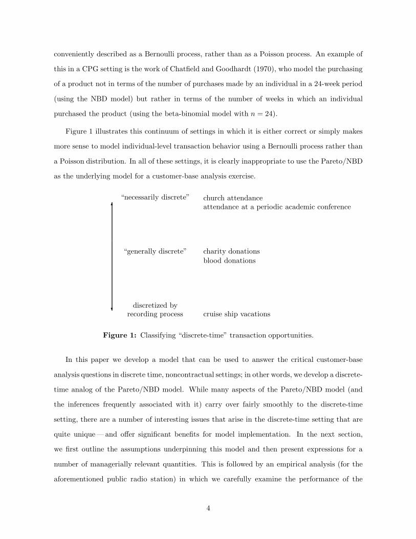
Figure 1 illustrates this continuum of settings in which it is either correct or simply makes

more sense to model individual-level transaction behavior using a Bernoulli process rather than

a Poisson distribution. In all of these settings, it is clearly inappropriate to use the Pareto/NBD

as the underlying model for a customer-base analysis exercise.

“necessarily discrete”

“generally discrete”

discretized byrecording process

6

?

church attendanceattendance at a periodic academic conference

charity donations

blood donations

cruise ship vacations

Figure 1: Classifying “discrete-time” transaction opportunities.

In this paper we develop a model that can be used to answer the critical customer-base

analysis questions in discrete time, noncontractual settings; in other words, we develop a discrete-

time analog of the Pareto/NBD model. While many aspects of the Pareto/NBD model (and

the inferences frequently associated with it) carry over fairly smoothly to the discrete-time

setting, there are a number of interesting issues that arise in the discrete-time setting that are

quite unique —and offer significant benefits for model implementation. In the next section,

we first outline the assumptions underpinning this model and then present expressions for a

number of managerially relevant quantities. This is followed by an empirical analysis (for the

aforementioned public radio station) in which we carefully examine the performance of the

4

model both in a six-year calibration sample and a five-year holdout period. We conclude with a

discussion of several additional issues that arise from this work.

2 Model Development

Our objective is to develop a stochastic model of buyer behavior for discrete-time, noncontractual

settings. To start, we define a transaction opportunity as either

• a well-defined point in time at which a transaction either occurs or does not occur, or

• a well-defined time interval during which a (single) transaction either occurs or does not

occur.

The first type of transaction opportunity corresponds to the “necessarily discrete” case in

Figure 1. The second type of transaction opportunity corresponds to the “generally discrete”

and “discretized by the recording process” cases in Figure 1. In all three cases, a customer’s

transaction history can be expressed as a binary string, where yt = 1 if a transaction occurred

at/during the tth transaction opportunity, 0 otherwise (for t = 1, . . . , n transaction opportuni-

ties). Note that we are simply interested in modeling the transaction process (i.e., the pattern of

1s and 0s). We are not interested in modeling other behaviors associated with each transaction

(e.g., the quantity purchased); this is discussed in Section 4.

Our model is based on the following six assumptions:

i. A customer’s relationship with the firm has two phases: he is “alive” (A) for some period

of time, then becomes permanently inactive (“dies”, D).

ii. While alive, the customer buys at any given transaction opportunity with probability p:

P (Yt = 1 | p, alive at t) = p .

(This implies that the number of transactions by a customer alive for n transaction op-

portunities follows a binomial distribution.)

5

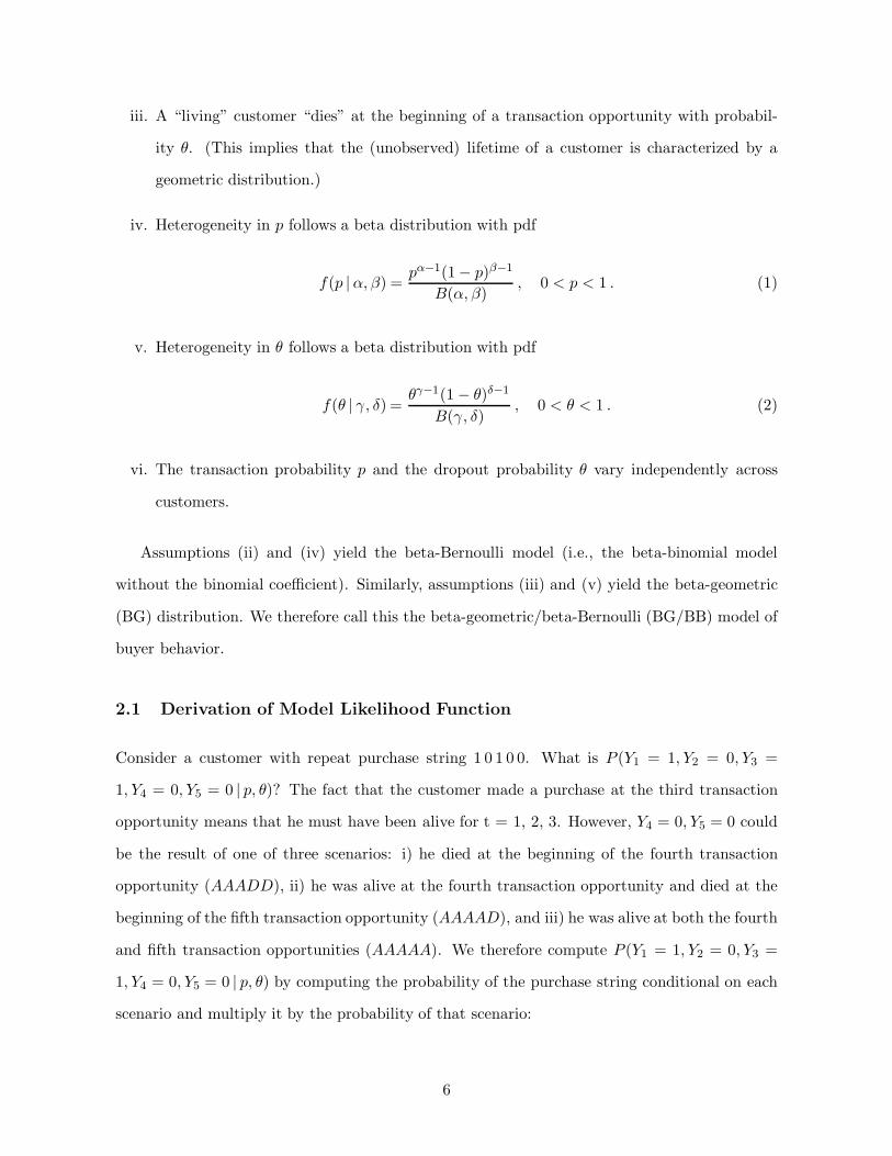
iii. A “living” customer “dies” at the beginning of a transaction opportunity with probabil-

ity θ. (This implies that the (unobserved) lifetime of a customer is characterized by a

geometric distribution.)

iv. Heterogeneity in p follows a beta distribution with pdf

f(p |α, β) =pα−1(1− p)β−1

B(α, β), 0 < p < 1 . (1)

v. Heterogeneity in θ follows a beta distribution with pdf

f(θ | γ, δ) =θγ−1(1 − θ)δ−1

B(γ, δ), 0 < θ < 1 . (2)

vi. The transaction probability p and the dropout probability θ vary independently across

customers.

Assumptions (ii) and (iv) yield the beta-Bernoulli model (i.e., the beta-binomial model

without the binomial coefficient). Similarly, assumptions (iii) and (v) yield the beta-geometric

(BG) distribution. We therefore call this the beta-geometric/beta-Bernoulli (BG/BB) model of

buyer behavior.

2.1 Derivation of Model Likelihood Function

Consider a customer with repeat purchase string 1 0 1 0 0. What is P (Y1 = 1, Y2 = 0, Y3 =

1, Y4 = 0, Y5 = 0 | p, θ)? The fact that the customer made a purchase at the third transaction

opportunity means that he must have been alive for t = 1, 2, 3. However, Y4 = 0, Y5 = 0 could

be the result of one of three scenarios: i) he died at the beginning of the fourth transaction

opportunity (AAADD), ii) he was alive at the fourth transaction opportunity and died at the

beginning of the fifth transaction opportunity (AAAAD), and iii) he was alive at both the fourth

and fifth transaction opportunities (AAAAA). We therefore compute P (Y1 = 1, Y2 = 0, Y3 =

1, Y4 = 0, Y5 = 0 | p, θ) by computing the probability of the purchase string conditional on each

scenario and multiply it by the probability of that scenario:

6

f(10100 | p, θ) = f(10100 | p,AAADD)P (AAADD | θ)

+ f(10100 | p,AAAAD)P (AAAAD | θ)

+ f(10100 | p,AAAAA)P (AAAAA | θ)

= p(1− p)p (1 − θ)3θ︸︷︷︸

P (AAADD)

+p(1 − p)p(1− p) (1 − θ)4θ︸︷︷︸

P (AAAAD)

+ p(1 − p)p︸︷︷︸

P (Y1=1,Y2=0,Y3=1)

(1− p)(1− p) (1 − θ)5︸︷︷︸

P (AAAAA)

(3)

Note that the zero-order nature of purchasing while the customer is alive means that the

exact order of any given number of transactions prior to the last observed transaction does not

matter. For example, it should be clear that f(10100 | p, θ) = f(01100 | p, θ). Therefore we do

not need the complete binary-string representation of a customer’s transaction history. Rather,

all we need to know for n transaction opportunities are frequency and recency : the number

of transactions across the calibration period (x =∑n

t=1 yt), and the transaction opportunity

at which the last observed transaction occurred (tx).2 We therefore go from 2n binary string

representations of all the possible purchase patterns to n(n+1)/2+1 possible recency/frequency

patterns.

This realization that recency and frequency are sufficient summary statistics offers signficant

benefits for model implementation, particularly as the number of transaction opportunities be-

comes sizeable. For instance, in the case of our public radio station, we can compress the number

of necessary binary strings from 64 down to 22 recency/frequency combinations, making it a bit

easier to visualize and manipulate the dataset. But in another recent application with n = 10,

we saw a reduction from 1024 binary strings down to 56 recency/frequency combinations. Fur-

thermore, these numbers are not affected by the size of the customer base being modeled; see

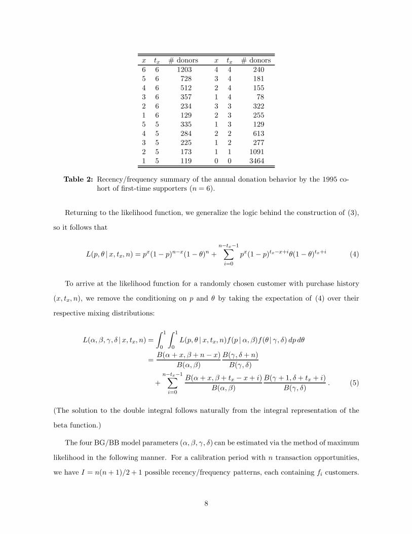
Table 2 for a complete characterization of the public radio dataset partially presented in Table 1.

Whether we have 11,000 customers or 11 million customers, the data structure is effectively iden-

tical— the numbers in the # donors columns would grow, but the computational demands for

data storage and manipulation are unchanged.

2If x = 0, then tx = 0. Note that this measure of recency differs from that normally used by the directmarketing community, who measure recency as the time from the last observed transaction to the end of theobservation period (i.e., n − tx).

7

x tx # donors x tx # donors

6 6 1203 4 4 2405 6 728 3 4 181

4 6 512 2 4 1553 6 357 1 4 78

2 6 234 3 3 3221 6 129 2 3 2555 5 335 1 3 129

4 5 284 2 2 6133 5 225 1 2 277

2 5 173 1 1 10911 5 119 0 0 3464

Table 2: Recency/frequency summary of the annual donation behavior by the 1995 co-hort of first-time supporters (n = 6).

Returning to the likelihood function, we generalize the logic behind the construction of (3),

so it follows that

L(p, θ | x, tx, n) = px(1− p)n−x(1 − θ)n +

n−tx−1∑

i=0

px(1 − p)tx−x+iθ(1 − θ)tx+i (4)

To arrive at the likelihood function for a randomly chosen customer with purchase history

(x, tx, n), we remove the conditioning on p and θ by taking the expectation of (4) over their

respective mixing distributions:

L(α, β, γ, δ | x, tx, n) =

∫ 1

0

∫ 1

0L(p, θ | x, tx, n)f(p |α, β)f(θ | γ, δ) dp dθ

=B(α + x, β + n − x)

B(α, β)

B(γ, δ + n)

B(γ, δ)

+

n−tx−1∑

i=0

B(α + x, β + tx − x + i)

B(α, β)

B(γ + 1, δ + tx + i)

B(γ, δ). (5)

(The solution to the double integral follows naturally from the integral representation of the

beta function.)

The four BG/BB model parameters (α, β, γ, δ) can be estimated via the method of maximum

likelihood in the following manner. For a calibration period with n transaction opportunities,

we have I = n(n + 1)/2 + 1 possible recency/frequency patterns, each containing fi customers.

8

The sample log-likelihood function is given by

LL(α, β, γ, δ) =

I∑

i=1

fi ln[L(α, β, γ, δ | xi, txi , n)

]

where xi and txi are the frequency and recency for each unique pattern. This can be maximized

using standard numerical optimization routines. These calculations are easy to perform in a

spreadsheet environment; in fact, the entire model implementation (from initial data setup

through the calculation of the “key results” in the next section) rarely requires the analyst to

use any software beyond a spreadsheet. This is a major benefit of the BG/BB model.

2.2 Key Results

We now present expressions for a set of quantities of interest to anyone wanting to apply this

model of buyer behavior in a discrete-time, noncontractual setting. (The associated derivations

can be found in the appendix.)

Let the random variable X(n) =∑n

t=1 Yt denote the number of transactions occurring across

the first n transaction opportunities. The BG/BB pmf is

P (X(n) = x |α, β, γ, δ) =

(n

x

)B(α + x, β + n − x)

B(α, β)

B(γ, δ + n)

B(γ, δ)

+n−1∑

i=x

(i

x

)B(α + x, β + i − x)

B(α, β)

B(γ + 1, δ + i)

B(γ, δ), (6)

with mean

E(X(n) |α, β, γ, δ) =

(α

α + β

)(1

γ − 1

){

δ −Γ(γ + δ)Γ(δ + n + 1)

Γ(δ)Γ(γ + δ + n)

}

. (7)

More generally, let the random variable X(n, n + n∗) =∑n∗

t=n+1 Yt denote the number of

transactions in the interval (n, n + n∗]. The BG/BB probability of x∗ transactions occurring in

this interval is given by

9

P (X(n, n + n∗) = x∗ |α, β, γ, δ) = δx∗=0

{

1 −B(γ, δ + n)

B(γ, δ)

}

+

(n∗

x∗

)B(α + x∗, β + n∗ − x∗)

B(α, β)

B(γ, δ + n + n∗)

B(γ, δ)

+

n∗−1∑

i=x∗

(i

x∗

)B(α + x∗, β + i − x∗)

B(α, β)

B(γ + 1, δ + n + i)

B(γ, δ), (8)

with mean

E(X(n, n + n∗) |α, β, γ, δ) =

(α

α + β

)(1

γ − 1

)

×

{Γ(γ + δ)Γ(δ + n + 1)

Γ(δ)Γ(γ + δ + n)−

Γ(γ + δ)Γ(δ + n + n∗ + 1)

Γ(δ)Γ(γ + δ + n + n∗)

}

. (9)

In most customer-base analysis settings we are interested in making statements about cus-

tomers conditional on their observed purchase history (x, tx, n).

• The probability that a customer with purchase history (x, tx, n) will be alive at the (n+1)th

transaction opportunity is

P (alive at n + 1 |α, β, γ, δ, x, tx, n)

=B(α + x, β + n − x)

B(α, β)

B(γ, δ + n + 1)

B(γ, δ)

/

L(α, β, γ, δ | x, tx, n) . (10)

• The probability that a customer with purchase history (x, tx, n) makes x∗ transactions in

the interval (n, n + n∗] is

P (X(n, n + n∗) = x∗ |α, β, γ, δ, x, tx, n)

= δx∗=0

{

1 −C1

L(α, β, γ, δ | x, tx, n)

}

+C2

L(α, β, γ, δ | x, tx, n)(11)

where

C1 =B(α + x, β + n − x)

B(α, β)

B(γ, δ + n)

B(γ, δ)

10

and

C2 =

(n∗

x∗

)B(α + x + x∗, β + n − x + n∗ − x∗)

B(α, β)

B(γ, δ + n + n∗)

B(γ, δ)

+

n∗−1∑

i=x∗

(i

x∗

)B(α + x + x∗, β + n − x + i − x∗)

B(α, β)

B(γ + 1, δ + n + i)

B(γ, δ).

• The expected number of future transactions across the next n∗ transaction opportunities

by a customer with purchase history (x, tx, n) is

E(X(n, n + n∗) |α, β, γ, δ, x, tx, n) =1

L(α, β, γ, δ | x, tx, n)

B(α + x + 1, β + n − x)

B(α, β)

×Γ(γ + δ)

(γ − 1)Γ(δ)

{Γ(δ + n + 1)

Γ(γ + δ + n)−

Γ(δ + n + n∗ + 1)

Γ(γ + δ + n + n∗)

}

. (12)

• We may also be interested in making inferences about a customer’s latent transaction and

dropout probabilities. The mean of the marginal posterior distribution of p is

E(P |α, β, γ, δ, x, tx, n) =

(α

α + β

)L(α + 1, β, γ, δ | x, tx, n)

L(α, β, γ, δ | x, tx, n), (13)

while the mean of the marginal posterior distribution of θ is

E(Θ |α, β, γ, δ, x, tx, n) =

(γ

γ + δ

)L(α, β, γ + 1, δ | x, tx, n)

L(α, β, γ, δ | x, tx, n). (14)

• Many customer-base analysis exercises are motivated by a desire to compute customer

lifetime value (CLV), which is “the present value of future cash flows attributed to the

customer relationship” (Pfeifer, Haskins, and Conroy 2005, p. 10). The general explicit

formula for computing CLV is (Rosset et al. 2003)

E(CLV ) =

∫ ∞

0

E[v(t)]S(t)d(t)dt ,

where E[v(t)] is the expected value of the customer at time t (assuming he is alive), S(t)

is the survivor function, and d(t) is a discount factor that reflects the present value of

money received at time t. Following Fader et al. (2005), if we assume that the process

11

describing the net cash flow per transaction for a given customer is both independent of the

transaction process and stationary, we can express v(t) as net cash flow / transaction×t(t),

where t(t) is the transaction rate at t.

In many cases we are interested in the expected residual lifetime of a customer. Standing

at time T ,

E(RLV ) = E(net cashflow/ transaction) ×

∫ ∞

T

E[t(t)]S(t | t > T )d(t− T )dt

︸︷︷︸

discounted expected residual transactions

.

The number of discounted expected residual transactions (DERT ) is the present value of

the expected future transaction stream for a customer with purchase history (x, tx, T ).

Fader et al. (2005) derive the expression for this quantity when the transaction process

can be described by the Pareto/NBD model. When the transaction process is described

by the BG/BB model, the present value of the expected number of future transactions for

a customer with purchase history (x, tx, n), with discount rate d is:3

DERT (d |α, β, γ, δ, x , tx, n) =B(α + x + 1, β + n − x)

B(α, β)

B(γ, δ + n + 1)

B(γ, δ)(1 + d)

×2F1

(1, δ + n + 1; γ + δ + n + 1; 1

1+d

)

L(α, β, γ, δ | x, tx, n). (15)

where 2F1(·) is the Gaussian hypergeometric function. This number of discounted expected

transactions can then be rescaled by the customer’s value multiplier to yield an overall

estimate of E(RLV ). While the presence of the Gaussian hypergeometric function makes

this calculation a bit more complex than the others in this section, it is worth emphasizing

that it only needs to be evaluated once for any given value of n (i.e., only once per co-

hort, not for every recency/frequency pattern) and it is relatively straightforward to use a

recursion formula to perform the calculations in a familiar spreadsheet environment. Fur-

thermore, this calculation for DERT is far simpler than the equivalent expression derived

by Fader et al. (2005) for the Pareto/NBD model. In that case, the DERT expression

3Suppose there are k transaction opportunities per year. An annual discount rate of r maps to a discount rateof d = (1 + r)1/k

− 1.

12

required the evaluation of the confluent hypergeometric function of the second kind, which

is more unfamiliar and burdensome (from a computational standpoint) than the Gaussian

hypergeometric function.

3 Empirical Analysis

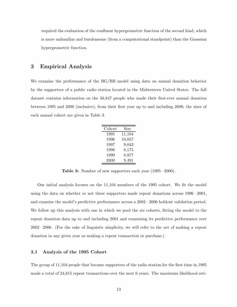
We examine the performance of the BG/BB model using data on annual donation behavior

by the supporters of a public radio station located in the Midwestern United States. The full

dataset contains information on the 56,847 people who made their first-ever annual donation

between 1995 and 2000 (inclusive), from their first year up to and including 2006; the sizes of

each annual cohort are given in Table 3.

Cohort Size

1995 11,1041996 10,057

1997 9,0431998 8,175

1999 8,9772000 9,491

Table 3: Number of new supporters each year (1995– 2000).

Our initial analysis focuses on the 11,104 members of the 1995 cohort. We fit the model

using the data on whether or not these supporters made repeat donations across 1996– 2001,

and examine the model’s predictive performance across a 2002 – 2006 holdout validation period.

We follow up this analysis with one in which we pool the six cohorts, fitting the model to the

repeat donation data up to and including 2001 and examining its predictive performance over

2002 – 2006. (For the sake of linguistic simplicity, we will refer to the act of making a repeat

donation in any given year as making a repeat transaction or purchase.)

3.1 Analysis of the 1995 Cohort

The group of 11,104 people that became supporters of the radio station for the first time in 1995

made a total of 24,615 repeat transactions over the next 6 years. The maximum likelihood esti-

13

mates of the model parameters are reported in Table 4.4 (We also report the model parameters

and value of the log-likelihood function for the beta-Bernoulli model, and note that the addition

of the “death” component results in a major improvement in model fit.)

α β γ δ LL

BB 0.487 0.826 −35,516.1

BG/BB 1.204 0.750 0.657 2.783 −33,225.6

Table 4: Parameter estimates, 1995 cohort.

The expected number of people making 0, 1, . . . , 6 repeat transactions between 1996 and

2001 is computed using (6) and compared to the actual frequency distribution in Figure 2. We

note that the model provides a very good fit to the data.

0 1 2 3 4 5 6

# Repeat Transactions

0

1,000

2,000

3,000

4,000

#Peo

ple

Actual

Model

Figure 2: Predicted versus actual frequency of repeat transactions.

The performance of the model becomes more impressive when we see how well it tracks repeat

transactions over time. Using the expression for the expected number of transactions across n

transaction opportunities as given in (7), we compute the expected number of repeat transactions

made by the whole cohort of 11,104 people up to 2006. These are plotted along with the actual

cumulative numbers in Figure 3a. We note that the BG/BB model predictions accurately track

the actual cumulative number of repeat transactions in both the six-year calibration period

and the five-year forecast period, underforecasting at 2006 by a mere −0.65%.5 Further insight

4Note that the entire analysis can easily be performed in a spreadsheet environment; copies of the Excelspreadsheets used to perform the analysis presented in this paper are available from the authors.

5As a point of comparison, the prediction associated with the BB model overforecasts cumulative repeattransactions at the end of 2006 by 20%.

14

into the excellent tracking performance of the model is given in Figure 3b, which reports these

numbers on a year-by-year basis; we note that the BG/BB model clearly captures the underlying

trend in repeat transactions over this fairly lengthy period of time.

1996 1997 1998 1999 2000 2001 2002 2003 2004 2005 2006

Year

0

10,000

20,000

30,000

40,000

Cum

ula

tive

#Rep

eat

Tra

nsa

ctio

ns

...........................................................................................................................................................................................................................................................................................................................................................................................................................................................................................................................................................................................................................................

×

×

×

×

×

×

×

×

×

×

×

Actual×

....

....

..

..

..

..

....

....

....

....

..

..

..

..

....

....

....

..

..

....

....

..

..

....

....

....

....

....

....

....

....

..

..

....

....

....

................................

....

........

....

................

....................

................................................................................................................................

�

�

�

�

�

�

�

��

��

Model�

(a)

1996 1997 1998 1999 2000 2001 2002 2003 2004 2005 2006

Year

0

1,000

2,000

3,000

4,000

5,000

6,000

#Rep

eat

Tra

nsa

ctio

ns

..................................................................................................................................................................................................................................................................................................................................................................................................................................................................................................................................................................................................................................

×

×

×

× ×

× ××

××

×

Actual×

....

....

....

....

....

....

....

....

....

....

....

....

....

....

....

........

....

............

................

................................................................................................

................

........................

............................................................................

�

�

�

��

��

� � � �

Model�

(b)

Figure 3: Predicted versus actual (a) cumulative and (b) annual repeat transactions.

To get a clearer idea of how well the model captures validation period purchasing, we compute

the expected number of people making x∗ = 0, 1, . . . , 5 transactions in 2002 – 2006 (n∗ = 5) using

(8) and compare it to the actual frequency distribution in Figure 4. We note that the model

provides a very good prediction of the actual behavior.

15

0 1 2 3 4 5


0

1,000

2,000

3,000

4,000

5,000

6,000

7,000

#Peo

ple

Actual

Model

Figure 4: Predicted versus actual frequency of repeat transactions in 2002 – 2006.

Conditional Expectations

Perhaps a more important examination of the predictive performance of the model focuses on

the quality of the predictions of future behavior conditional on past behavior. We use (12) to

compute the expected number of transactions in the 2002 – 2006 period (n∗ = 5) conditional on

each of the 22 (x, tx) patterns associated with n = 6. These conditional expectation are reported

in Table 5 as a function of recency (the year of the individual’s last transaction) and frequency

(the number of repeat transactions).

# Rpt Transactions Year of Last Transaction

(1996– 2001) 1995 1996 1997 1998 1999 2000 2001

0 0.071 0.09 0.31 0.59 0.84 1.02 1.15

2 0.12 0.54 1.06 1.44 1.673 0.22 1.03 1.80 2.19

4 0.58 2.03 2.715 1.81 3.23

6 3.75

Table 5: Expected number of repeat transactions in 2002– 2006 as a function of recency

and frequency.

In Figure 5a we report these conditional expectations along with the average of the number

of the transactions that actually occurred in the 2002 – 2006 forecast period, broken down by

the number of repeat transactions in 1996– 2001. (For each x, we are averaging over customers

16

with different values of tx.) Similarly, Figure 5b reports these conditional expectations along

with the average of the number of the transactions that actually occurred in the 2002 – 2006

forecast period, broken down by the year of the individual’s last transaction. (For each tx, we

are averaging over customers with different values of x.) We observe that the BG/BB model

generates very good predictions of the expected behavior in the longitudinal holdout period,

with the only real blemish being an underestimation of expected purchasing by those individuals

whose last repeat purchase occurred before 1998.

0 1 2 3 4 5 6

# Repeat Transactions (1996 – 2001)

0

1

2

3

4

#Rep

eat

Tra

nsa

ctio

ns

(2002

–2006)

...................................................................................................................................................................................................................................................................................................................................................................................................................................................................................................................................................................

×

×

×

×

×

×

×Actual×

........................................................

................................

....

....

....

....

....

....

....

....

....

....

....

....

....

....

..

..

....

....

..

..

....

..

..

.

..

.

....

..

..

....

....

..

..

..

.

.

....

..

..

..

..

....

.

..

.

..

..

....

..

.

.

.

...

....

..

..

.

..

.

..

.

.

..

..

.

..

.

..

.

.

..

..

.

..

.

....

..

..

.

..

.

..

.

.

....

..

..

..

.

.

..

..

��

�

�

�

�

�

Model�

(a)

1995 1996 1997 1998 1999 2000 2001

Year of Last Transaction

0

1

2

3

4

#Rep

eat

Tra

nsa

ctio

ns

(2002

–2006)

.........................................

......................................

......................................................................................................................................................................................................................................................................................................................................................................................................................................................................................

× ×

××

×

×

×

Actual×

............................................

............

............

............

............................................

............

....

................

....

........

....

..

..

.

..

.

.

...

..

..

..

..

....

..

.

.

..

.

.

....

..

..

..

..

..

..

....

..

..

.

..

.

..

.

.

..

..

.

..

.

..

..

.

..

.

..

.

.

..

..

.

..

.

..

..

.

..

.

..

..

.

..

.

..

.

.

..

..

.

..

.

..

..

� � ��

�

�

�Model�

(b)

Figure 5: Predicted versus actual conditional expectations of repeat transactions in2002– 2006 as a function of (a) frequency and (b) recency.

Referring back to Table 5, we can now address the questions about different kinds of cus-

tomers raised at the outset of the paper.

17

• A donor who has made repeat transactions at every possible opportunity is expected to

make “only” 3.75 transactions over the next five years. Of course, such donors are still

extremely valuable, but the possibility of “death” plus the fact that they might have

been somewhat lucky in the past make them a bit less valuable than they might have

otherwise seemed. (With reference to Figure 5a, we see that this conditional expectation

overestimates the actual mean (3.53) by only 6%.)

• Donor 100009, who had a perfect record until the most recent year, is expected to make

1.81 transactions over the next five years. In contrast, donor 100004, with better recency

but lower frequency, is expected to make 2.71 transactions over the same period —an

increase of nearly 50%! This highlights the critically important role of recency, which can

be also seen in the steep growth of the curve in Figure 5b.

• Although donors 100004 and 111103 have different histories, their recency and frequency

numbers are identical (x = 4, tx = 6); thus, they have the same conditional expectation.

Minor, remote differences in purchase histories are deemed to be irrelevant when making

predictions using the BG/BB model.

• A donor who has been completely absent since making their initial transaction is expected

to make only 0.07 repeat transactions over the next five years. But while each such donor

is not particularly valuable alone, it is important to note, as per Table 2, that over 30%

of the entire cohort of donors is in this recency/frequency group. Taken together, these

donors are expected to make over 240 transactions over the next five years, making them

collectively more valuable than about half of the other recency/frequency groups.

Beyond these specific analyses, Table 5 offers additional insights about the broader interplay

between recency and frequency. First, note that for any row (i.e., value of x), the expected

number of transactions in the forecast period decreases as we move from right to left (i.e., the

less recent the last observed transaction). This is as we would expect, since the longer the

hiatus in making a purchase, the more likely it is that the customer is “dead”. Looking down

the columns, however, we see a somewhat different pattern. We first look at 2001 and note that

the conditional expectation is clearly an increasing function of the number of repeat transactions

18

made in the six-year calibration period. Looking at the 1997 – 2000 columns, though, we note

that the numbers first increase then decrease as the number of repeat transactions made in

the six-year calibration period decreases. (A similar pattern is observed in the DERT numbers

under the Pareto/NBD model reported in Fader et al. (2005).)

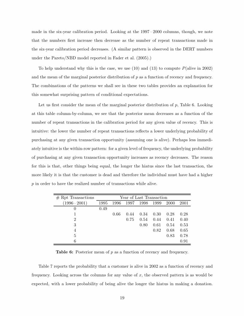
To help understand why this is the case, we use (10) and (13) to compute P (alive in 2002)

and the mean of the marginal posterior distribution of p as a function of recency and frequency.

The combinations of the patterns we shall see in these two tables provides an explanation for

this somewhat surprising pattern of conditional expectations.

Let us first consider the mean of the marginal posterior distribution of p, Table 6. Looking

at this table column-by-column, we see that the posterior mean decreases as a function of the

number of repeat transactions in the calibration period for any given value of recency. This is

intuitive: the lower the number of repeat transactions reflects a lower underlying probability of

purchasing at any given transaction opportunity (assuming one is alive). Perhaps less immedi-

ately intuitive is the within-row pattern: for a given level of frequency, the underlying probability

of purchasing at any given transaction opportunity increases as recency decreases. The reason

for this is that, other things being equal, the longer the hiatus since the last transaction, the

more likely it is that the customer is dead and therefore the individual must have had a higher

p in order to have the realized number of transactions while alive.


(1996– 2001) 1995 1996 1997 1998 1999 2000 2001

0 0.49

1 0.66 0.44 0.34 0.30 0.28 0.282 0.75 0.54 0.44 0.41 0.40

3 0.80 0.61 0.54 0.534 0.82 0.68 0.655 0.83 0.78

6 0.91

Table 6: Posterior mean of p as a function of recency and frequency.

Table 7 reports the probability that a customer is alive in 2002 as a function of recency and

frequency. Looking across the columns for any value of x, the observed pattern is as would be

expected, with a lower probability of being alive the longer the hiatus in making a donation.

19

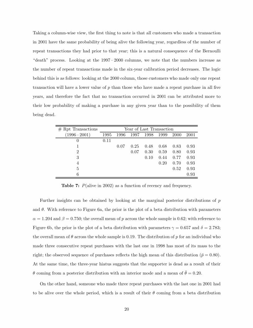
Taking a column-wise view, the first thing to note is that all customers who made a transaction

in 2001 have the same probability of being alive the following year, regardless of the number of

repeat transactions they had prior to that year; this is a natural consequence of the Bernoulli

“death” process. Looking at the 1997– 2000 columns, we note that the numbers increase as

the number of repeat transactions made in the six-year calibration period decreases. The logic

behind this is as follows: looking at the 2000 column, those customers who made only one repeat

transaction will have a lower value of p than those who have made a repeat purchase in all five

years, and therefore the fact that no transaction occurred in 2001 can be attributed more to

their low probability of making a purchase in any given year than to the possibility of them

being dead.


(1996– 2001) 1995 1996 1997 1998 1999 2000 2001

0 0.11

1 0.07 0.25 0.48 0.68 0.83 0.932 0.07 0.30 0.59 0.80 0.93

3 0.10 0.44 0.77 0.934 0.20 0.70 0.935 0.52 0.93

6 0.93

Table 7: P (alive in 2002) as a function of recency and frequency.

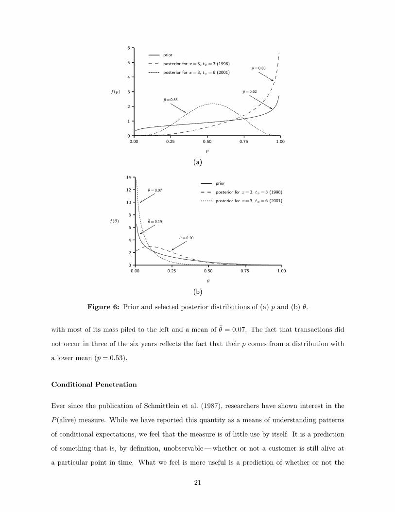
Further insights can be obtained by looking at the marginal posterior distributions of p

and θ. With reference to Figure 6a, the prior is the plot of a beta distribution with parameters

α = 1.204 and β = 0.750; the overall mean of p across the whole sample is 0.62; with reference to

Figure 6b, the prior is the plot of a beta distribution with parameters γ = 0.657 and δ = 2.783;

the overall mean of θ across the whole sample is 0.19. The distribution of p for an individual who

made three consecutive repeat purchases with the last one in 1998 has most of its mass to the

right; the observed sequence of purchases reflects the high mean of this distribution (p̄ = 0.80).

At the same time, the three-year hiatus suggests that the supporter is dead as a result of their

θ coming from a posterior distribution with an interior mode and a mean of θ̄ = 0.20.

On the other hand, someone who made three repeat purchases with the last one in 2001 had

to be alive over the whole period, which is a result of their θ coming from a beta distribution

20

0.00 0.25 0.50 0.75 1.00

p

0

1

2

3

4

5

6

f(p)

...................................................................................................

...........................

...............................

.................................

.................................

.................................

................................

...............................

............................

................................................................................................................................................................................................................................................................................................

prior

............. ............. ............. ..........................

.............

.............

.............

.............

.............

.............

.............

.............

.............

.............

.............

.............

.............

..

...........

.............

..

...........

..

..

..

.......

..

..

..

.

..

..

.

.

..

..

..

..

.

.

..

.

..

..

..

..

.

..

..

.

..

..

.

..

.

..

..

..

..

.

..

.

..

.

..

.

.

..

.

..

.

..

.

..

..

.

..

.

..

.

..

.

.

.

..

.

posterior for x =3, tx = 3 (1998)

................................................................

....

....

....

....

..

..

....

....

....

....

..

..

..

..

....

....

....

..

..

....

........

....

........

............................

........................................

....

....

....

....

....

....

....

....

.

...

....

....

....

....

....

....

....

....

....

....

........

..................................

posterior for x =3, tx = 6 (2001)

......................................................................................................................

p̄= 0.62

.....................................................................................

p̄= 0.80

.....................................................................................

p̄= 0.53

(a)

0.00 0.25 0.50 0.75 1.00

θ

0

2

4

6

8

10

12

14

f(θ)...................................................................................................................................................................................................................................................................................................................................................................................................................................................................................................................................................................................................................................................................................

prior

.............

.............

..........................

.............

.............

.............

.............

.............

.............

.............

.............

..........................

............. ............. ............. ............. ............. ............. ............. .............

posterior for x =3, tx =3 (1998)

.

..

.

..

.

.

.

..

.

.

.

..

..

.

.

.

.

..

..

.

.

.

..

.

..

.

.

.

..

.

.

.

..

..

.

.

.

.

..

..

.

.

.

..

.

.

.

..

..

.

.

.

..

.

.

.

..

..

.

.

.

..

.

.

..

.

.

.

..

..

.

.

..

.

.

..

.

.

.

..

.

..

.

.

..

..

.

.

..

.

..

.

..

..

..

..

.

...

..

..

....

..

..

....

....

....

....

....

....

....

....

................................................................................................................................................................................................

posterior for x =3, tx =6 (2001)

............................................................................

.........

θ̄ = 0.19

............................................................................

.........

θ̄ = 0.20

............................................................................

.........

θ̄ = 0.07

(b)

Figure 6: Prior and selected posterior distributions of (a) p and (b) θ.

with most of its mass piled to the left and a mean of θ̄ = 0.07. The fact that transactions did

not occur in three of the six years reflects the fact that their p comes from a distribution with

a lower mean (p̄ = 0.53).

Conditional Penetration

Ever since the publication of Schmittlein et al. (1987), researchers have shown interest in the

P (alive) measure. While we have reported this quantity as a means of understanding patterns

of conditional expectations, we feel that the measure is of little use by itself. It is a prediction

of something that is, by definition, unobservable —whether or not a customer is still alive at

a particular point in time. What we feel is more useful is a prediction of whether or not the

21

customer will be active in the future, that is, whether or not the customer undertakes any

transactions in a specified future period of time.6

The probability that a customer is active in the 2002 – 2006 period (n∗ = 5) is computed

as 1 − P (X(n, n + n∗) = 0 | x, tx, n) using (11), conditional on each of the 22 (x, tx) patterns

associated with n = 6. This conditional penetration is reported in Table 8 as a function of

recency (the year of the individual’s last transaction) and frequency (the number of repeat

transactions).


(1996– 2001) 1995 1996 1997 1998 1999 2000 2001

0 0.05

1 0.05 0.17 0.32 0.46 0.56 0.622 0.05 0.24 0.48 0.66 0.76

3 0.09 0.40 0.69 0.844 0.19 0.66 0.88

5 0.51 0.916 0.92

Table 8: Probability of being active in 2002– 2006 as a function of recency and frequency.

Comparing Tables 5 and 8, we note that the estimated probabilities of being alive in 2002

are strictly higher than the corresponding conditional 2002 – 2006 penetration numbers. This

makes intuitive sense, but the differences between these measures reflect several factors. First,

the P (alive) numbers are just for one year, whereas the penetration numbers are for a five-

year period. Second, the mere fact that someone is alive does not mean she will be active,

as the latter state depends on the person’s underlying transaction probability p. This is very

clear when we look at the right-most column of both tables. While those people who made

a purchase in 2001 have the same probability of being alive, irrespective of frequency, their

corresponding probabilities of making at least one transaction in the next five years clearly

(and logically) decrease as a function of frequency, reflecting in part the lower probabilities of

making a purchase at any given transaction opportunity given alive (Table 6). Third, the lower

penetration numbers also reflect the fact that inactivity may be due to the person dying in

6Many authors, including Schmittlein et al. (1987), have used the terms “alive” and “active” as synonyms.We feel that this should not be the case, with the term “alive” referring to an unobservable state and the term“active” referring to observable behavior.

22

2003 – 2006, even if they were alive in 2002.

In summary, we encourage researchers who might be attracted by the P (alive) measure to

focus on the conditional penetration numbers instead, since they reflect an observable quantity

(i.e., whether or not the customer is active).

3.2 Pooled Analysis

The analyses presented above all focused on a single cohort, the group of individuals who made

their first-ever donation during 1995. However, as noted earlier, we have data for a total of six

cohorts. At first glance we may be tempted to apply the model cohort by cohort; unfortunately

we are not able to estimate a complete set of cohort-specific parameters. Consider, for instance,

the 2000 cohort: we only have one observation per customer —whether or not each new donor

made a repeat donation in 2001 (i.e., n = 1)—and as such cannot identify the model parameters.

The obvious, albeit possibly restrictive, solution is to pool all six cohorts and estimate a single

set of model parameters. We now turn our attention to such an analysis, examining how well

the BG/BB model predicts the behavior of the complete group of the 56,847 people who made

their first-ever donation to the radio station between 1995 and 2000.

The maximum likelihood estimates of the model parameters are reported in Table 9. (Com-

paring the fit of the BG/BB model with that of the beta-Bernoulli model, we once again note

that the addition of the “death” component results in a major improvement in model fit.) We

also note that the BG/BB parameters for the pooled model are remarkably similar to those of

the 1995 cohort by itself (Table 4)— this reflects both the high reliability of the model as well

as the “poolability” of the cohorts. Figure 7, which compares the expected number of people

making 0, 1, . . . , 6 repeat transactions between 1996 and 2001 with the observed frequencies,

confirms that the model provides a very good fit to the data.

α β γ δ LL

BB 0.501 0.753 −115,615.0BG/BB 1.188 0.749 0.626 2.331 −110,521.0

Table 9: Parameter estimates, pooling the 1995 – 2000 cohorts.

23

0 1 2 3 4 5 6


0

5,000

10,000

15,000

20,000

25,000

#Peo

ple

Actual

Model

Figure 7: Predicted versus actual frequency of repeat transactions by the 1995– 2000

cohorts.

The pooled model continues to accurately track the actual number of repeat transactions

over time. Viewing Figure 8a, which shows the actual vs. predicted cumulative number of

repeat transactions, we see that the model overforecasts the holdout transactions by a mere

0.25%. Looking at Figure 8b, which reports these numbers on a year-by-year basis, we note that

the BG/BB model clearly captures the underlying trend in repeat transactions. (The repeat

transaction numbers rise up to 2001, as new supporters continue to enter the combined pool of

donors; after that point, we are focusing on a fixed group of 56,847 potential repeat supporters.)

The conditional expectation plots, omitted in the interests of space, are similarly impressive.

This pooled analysis provides a further illustration of the remarkable ability of the BG/BB

model to describe and predict the future behavior of a customer base. It is encouraging to

see how one set of parameters can capture the behavior of different cohorts acquired across six

consecutive years (1995– 2000) and project their actions quite accurately into the future.

4 Discussion

We have developed a new model that can be used to answer standard customer-base analy-

sis questions in noncontractual settings where opportunities for transactions occur at discrete

intervals (i.e., a discrete-time analog of the Pareto/NBD model). Using a dataset on annual

donations made by the supporters of a public radio station located in the Midwestern United

24

1996 1997 1998 1999 2000 2001 2002 2003 2004 2005 2006

Year

0

40,000

80,000

120,000

160,000

Cum

ula

tive

#Rep

eat

Tra

nsa

ctio

ns

................................................................................................................................................................................................................................................................................................................................................................................................................................................................................................................................................................................................................................................................

×

×

×

×

×

×

×

×

×

×

×

Actual×

....................................

............

............

....

....

........

....

....

..

..

....

....

..

..

....

....

....

....

....

..

..

..

..

....

....

..

..

....

....

..

.

.

....

..

..

..

..

....

..

..

..

..

..

..

....

....

....

....

....

....

....

..

..

....

....

....

....

..

..

....

....

........

....

..

..

....

....

....

....

....

..

..

............

....

....

....

....

....

....

....

................

....

��

�

�

�

�

�

�

�

�

�

Model�

(a)

1996 1997 1998 1999 2000 2001 2002 2003 2004 2005 2006

Year

0

5,000

10,000

15,000

20,000

#Rep

eat

Tra

nsa

ctio

ns

..

..

..

.......................................................................................................................................................................................................................................................................................................................................................................................................................................................................................................................................................................................................................................

......................................................................................

×

×

×

×

×

×

×

×

×

×

×

Actual×

..

.

.

.

..

.

.

..

.

.

..

.

.

..

.

.

..

.

..

..

..

..

..

..

..

..

..

.

.

..

.

.

....

.

...

..

..

..

..

..

..

..

..

.

..

.

....

..

..

..

..

..

..

....

....

....

....

....

..

..

..

..

..

..

..

..

....

..

..

....

..

..

....

..

..

....

..

..

....

..

..

....

..

..

....

..

..

....

..

..

.

...

..

..

....

....

....

....

....

....

....

....

....

............

....

....

....

.....................................................................................................

�

�

�

�

�

�

�

��

��

Model�

(b)

Figure 8: Predicted versus actual (a) cumulative and (b) annual repeat transactions.

States, we have demonstrated how the model can be used to compute a number of managerially

relevant quantities, such as future purchasing patterns, both collectively and individually (con-

ditional on past behavior). In examining these quantities, we have observed some interesting

effects of past behavior (as summarized by recency and frequency) on predictions about future

behavior.

It is worthwhile to contrast the BG/BB with the Pareto/NBD model and some of the equiv-

alent analyses performed using it (e.g., in studies such as Fader et al. (2005)). First, as we men-

tioned right from the outset of this paper, the BG/BB is the direct analog of the Pareto/NBD

as one moves from a continuous-time setting to a discrete-time domain. We have brought up

25

a number of specific examples where this distinction is critically important, as well as some

situations (characterized as “discretized by recording process” in Figure 1) where the analyst

might intentionally convert a continuous-time setting into a discrete-time one primarily to be

able to use the BG/BB model instead of the Pareto/NBD. We are aware of several organizations

(including hotel chains, financial services firms, and a variety of non-profits) that have chosen

this route. The fact that they have done so is an indication of the unique benefits associated

with this new model.

These benefits have been mentioned throughout the paper, but we summarize them here:

• The BG/BB offers tremendous advantages in terms of the required data structures. The

size of the data summary required for model estimation is purely a function of the number

of transaction opportunities—not the number of customers—and therefore the model is

highly “scalable” to customer bases of different sizes. Furthermore, in recognizing that re-

cency and frequency are sufficient summary statistics, the relationship between the number

of transaction opportunities and the size of the dataset is on the order of n2, which is a

significant reduction compared to using the full binary strings (order 2n).

• Besides the efficient data requirements, the calculations associated with the model are

much simpler than those of the Pareto/NBD. No unconventional or computationally de-

manding functions are required for parameter estimation or for most of the diagnostic

statistics that emerge from the model. Taken together with the aforementioned data ad-

vantages, this means that the model is easy to fully implement and utilize within a standard

spreadsheet environment. This is very appealing to practitioners, since this reduction in

space/effort can be accomplished at virtually no cost (i.e., without sacrificing anything in

model performance, as shown in our empirical analyses).

• The discrete nature of the data and the associated behavioral “story” lead to model diag-

nostics that are convenient to display and are readily interpretable. For instance it is very

easy to see and appreciate the non-linear pattern associated with high frequency and low

recency, shown in Table 5. Likewise, a simple examination of that table instantly answers

the managerial questions raised in the introduction.

26

• Finally, it is relatively easy to build and analyze the BG/BB model across multiple cohorts

of customers —something that has been done rarely (if ever) in the Pareto/NBD literature.

Not only does this make the model even more practical, but the multi-year empirical

results shown here offer much stronger support for the model’s validity than a single-

cohort analysis can provide.

While the BG/BB is an excellent starting point for modeling discrete-time noncontractual

data, there are several natural extensions worth investigating in future research. First, as is the

case with the Pareto/NBD model, the BG/BB model will need to be augmented by a model of

purchase amounts when we are interested in the overall monetary value of each customer. A

natural candidate would be the gamma-gamma mixture (Colombo and Jiang 1999) that Fader

et al. (2005) use in conjunction with the Pareto/NBD model. In situations where the data

have been discretized for analysis and reporting purposes, there is the possibility that more

than one transaction could occur in each discrete time interval. In such cases, we should derive

the monetary-value multiplier by first modeling the number of transactions (conditional on

the fact that at least one transaction occurred) and then multiply this by the average value

per transaction. A logical model would be the shifted beta-geometric distribution (as used by

Morrison and Perry (1970) to model purchase quantity, conditional on purchase incidence).

Second, we may want to allow for a non-zero-order purchasing process at the individual level.

A good historical starting point would be the “Brand Loyal Model” (Massy, Montgomery, and

Morrison 1970). This would effectively be an extension of Morrison et al.’s (1982) Markov chain

model of retail customer behavior at Merrill Lynch; an extension in which the “exit parameter”

is allowed to be heterogeneous and is estimated directly from the data (as opposed to being

derived from other data sources).

Finally, the model can be extended to include covariate effects, such as customer demo-

graphics, marketing actions, and measures of competitive activity. It would be worthwhile to

find out which kinds of marketing actions increase buying propensities while the customer is

“alive,” in contrast to actions that primarily serve to stretch out the customer’s probable life-

time. Such a decomposition could have huge implications for developing marketing plans and

allocating resources. In bringing in covariates, it will likely be necessary to move away from the

27

simple spreadsheet-based model implementation featured here towards a more complex hierar-

chical Bayes framework. This would enable additional benefits (such as allowing for correlations

between the two underlying behavioral processes) but also comes at a cost (i.e., speed and con-

venience of model estimation, loss of closed-form expressions for key model-derived measures,

and the loss of the simple recency/frequency data structure whose size is independent of the

number of people in the sample). But it makes sense to develop such a model and weigh the

associated tradeoffs.

But even when these extensions are undertaken, the BG/BB model in its basic form should

still serve as an appropriate benchmark model; furthermore, the diagnostic statistics discussed

here should continue to be utilized in evaluating the overall performance of the model as well

as the incremental value of any additions that might be brought into it. It might be hard for

researchers to improve upon the results shown here, but we sincerely encourage the development

and testing of richer models to help us gain an even better understanding of customer behavior

in the discrete-time, noncontractual setting.

28

Appendix

In this appendix we present derivations of the key results presented in Section 2.2. Before

starting, we first recall that for 0 < k < 1,

• the sum of the first n terms of a geometric series is

a + ak + ak2 + · · ·akn−1 = a1 − kn

1 − k, (A1)

• the sum of an infinite geometric series is

∞∑

n=0

akn =a

1− k, (A2)

and note the following transformation of Euler’s integral representation of the Gaussian hyper-

geometric function (2F1(a, b; c; z)):

∫ 1

0

tb−1(1− t)c−b−1(1− zt)−adt = B(b, c− b)2F1(a, b; c; z) , c > b . (A3)

A.1 Derivation of (6)

An individual making x purchases had to be alive for at least the first x transactions opportu-

nities. Conditional on p, the probability of observing x transactions out of the i (unobserved)

transaction opportunities (i = x, . . . , n) the customer is alive is

(i

x

)

px(1− p)i−x .

Removing the conditioning on being alive for i transaction opportunities by multiplying this

by the probability that the individual is alive for that length of time give us

P (X(n) = x | p, θ) =

(n

x

)

px(1 − p)n−x(1− θ)n +

n−1∑

i=x

(i

x

)

px(1− p)i−xθ(1 − θ)i . (A4)

Taking the expectation of this over the mixing distributions for p and θ ((1) and (2), respec-

tively) gives us (6).

29


Conditional on p and θ, the expected number of transactions over n transaction opportunities

is computed as

E(X(n) | p, θ) =

n∑

t=1

P (Yt = 1 | p, alive at t)P (alive at t | θ)

= pn∑

t=1

(1 − θ)t

= p(1 − θ)

n−1∑

s=0

(1− θ)s ,

which, recalling (A1) and performing some further algebra,

=p(1 − θ)

θ−

p(1− θ)n+1

θ. (A5)

Taking the expectation of this over the mixing distributions for p and θ gives us

E(X(n) |α, β, γ, δ) =

(α

α + β

) {B(γ − 1, δ + 1) − B(γ − 1, δ + n + 1)

B(γ, δ)

}

.

(Strictly speaking, the use of the integral representation of the beta function to solve the integral

associated with taking the expectation over θ only holds for γ > 1. However it can be shown

that we arrive at the same result when 0 < γ < 1.) Representing the beta functions in terms of

gamma functions and recalling the recursive property of gamma functions gives us (7).

A.3 Derivation of (8) and (9)

Recalling (A4), it follows from the memoryless nature of the death process that

P (X(n, n + n∗) = x∗ | p, θ, alive at n) =

(n∗

x∗

)

px∗

(1− p)n∗−x∗

(1− θ)n∗

+

n∗−1∑

i=x∗

(i

x∗

)

px∗

(1 − p)i−x∗

θ(1 − θ)i . (A6)

30

Noting that the probability that someone is alive at n is (1− θ)n, we have

P (X(n, n + n∗) = x∗ | p, θ) = δx∗=0

{

1− (1− θ)n}

+

(n∗

x∗

)

px∗

(1 − p)n∗−x∗

(1− θ)n+n∗

+

n∗−1∑

i=x∗

(i

x∗

)

px∗

(1 − p)i−x∗

θ(1 − θ)n+i .

(The first term accounts for the fact that anyone not alive at n will, by definition, not make any

purchases in the interval (n, n+n∗].) Taking the expectation of this over the mixing distributions

for p and θ gives us (8).

By definition, X(n, n+ n∗) = X(n+ n∗)−X(n); it follows that E[X(n, n+ n∗)] = E[X(n+

n∗)] − E[X(n)]. Substituting (7) in this gives us (9).


Reflecting on (4), the first term is the likelihood of x purchases out of n transaction opportunities

under the assumption that the customer was alive for all n transaction opportunities. (The other

terms account for the possibility that the individual died before n.) Using Bayes’ theorem, it

follows that the probability that a customer with purchase history (x, tx, n) is alive at n is

P (alive at n | p, θ, x, tx, n) =px(1− p)n−x(1 − θ)n

L(p, θ | x, tx, n). (A7)

It follows that

P (alive at n + 1 | p, θ, x, tx, n) =px(1 − p)n−x(1− θ)n+1

L(p, θ | x, tx, n). (A8)

By Bayes’ theorem, the joint posterior distribution of p and θ is given by

f(p, θ |α, β, γ, δ, x, tx, n) =L(p, θ | x, tx, n)f(p |α, β)f(θ | γ, δ)

L(α, β, γ, δ | x, tx, n), (A9)

where the individual elements are given in (1), (2), (4), and (5).

Taking the expectation of (A8) over the joint posterior distribution of p and θ, (A9), gives

us (10).

By the same logic, we can derive an expression for the probability that a customer with

31

purchase history (x, tx, n) is alive at transaction opportunity n + m. Conditional on p and θ,

P (alive at n + m | p, θ, x, tx, n) =px(1 − p)n−x(1− θ)n+m

L(p, θ | x, tx, n).

Taking the expectation of this over the joint posterior distribution of p and θ yields

P (alive at n + m |α, β, γ, δ, x, tx, n)

=B(α + x, β + n − x)

B(α, β)

B(γ, δ + n + m)

B(γ, δ)

/

L(α, β, γ, δ | x, tx, n) . (A10)


By definition,

P (X(n,n + n∗) = x∗ | p, θ, x, tx, n) = δx∗=0

{

1 − P (alive at n | p, θ, x, tx, n)}

+ P (X(n, n + n∗) = x∗ | p, θ, alive at n)P (alive at n | p, θ, x, tx, n) .

Substituting (A6) and (A7) in this, and taking the expectation over the joint posterior distri-

bution of p and θ, (A9), gives us (11).


Conditional on p and θ, the expected number of transactions across the next n∗ transaction

opportunities (i.e., in the interval (n, n + n∗]) by a customer with purchase history (x, tx, n) is

E(X(n, n + n∗) | p, θ, x, tx, n)

= E(X(n, n + n∗) | p, θ, alive at n) × P (alive at n | p, θ, x, tx, n) .

Now

E(X(n, n+ n∗) |p, θ, alive at n)

=

n+n∗

∑

t=n+1

P (Yt = 1 | p, alive at t)P (alive at t | θ, t > n)

32

= p

n+n∗

∑

t=n+1

(1− θ)t

(1− θ)n

= p

n∗

∑

s=1

(1 − θ)s

=p(1− θ)

θ−

p(1− θ)n∗+1

θ. (A11)

Taking the expectation of the product of (A7) and (A11) over the joint posterior distribution

of p and θ, (A9), gives us (12).

A.7 Derivation of (13) and (14)

Integrating (A9) over θ gives us the marginal posterior distribution of p:

f(p |α, β, γ, δ, x, tx, n) = A/L(α, β, γ, δ | x, tx, n) (A12)

where

A =pα+x−1(1− p)β+n−x−1

B(α, β)

B(γ, δ + n)

B(γ, δ)

+

n−tx−1∑

i=0

pα+x−1(1− p)β+tx−x+i−1

B(α, β)

B(γ + 1, δ + tx + i)

B(γ, δ).

(This equation was used to create the curves in Figure 6a.)

Integrating (A9) over p gives us the marginal posterior distribution of θ:

f(θ |α, β, γ, δ, x, tx, n) = B/L(α, β, γ, δ | x, tx, n) (A13)

where

B =B(α + x, β + n − x)

B(α, β)

θγ−1(1 − θ)δ+n−1

B(γ, δ)

+

n−tx−1∑

i=0

B(α + x, β + tx − x + i)

B(α, β)

θγ(1− θ)δ+tx+i−1

B(γ, δ).

33

(This equation was used to create the curves in Figure 6b.)

We note that when tx = n, (A12) and (A13) both collapse to the following beta distributions:

f(p |α, β, γ, δ, x, tx, n) =pα+x−1(1 − p)β+n−x−1

B(α + x, β + n − x)

f(θ |α, β, γ, δ, x, tx, n) =θγ−1(1− θ)δ+n−1

B(γ, δ + n).

In order to derive an expression for the mean of the marginal posterior distribution of p, we

could solve∫ 1

0pf(p |α, β, γ, δ, x, tx, n) dp .

However, a simpler derivation is as follows:

E(P |α, β, γ, δ, x, tx, n) =

∫ 1

0

∫ 1

0pf(p, θ |α, β, γ, δ, x, tx, n) dp dθ

which, recalling (A9)

=

∫ 1

0

∫ 1

0

pL(p, θ | x, tx, n)f(p |α, β)f(θ | γ, δ)

L(α, β, γ, δ | x, tx, n)dp dθ

=B(α + 1, β)

B(α, β)

∫ 1

0

∫ 1

0

L(p, θ | x, tx, n)f(p |α + 1, β)f(θ | γ, δ)


=

(α

α + β

)L(α + 1, β, γ, δ | x, tx, n)

L(α, β, γ, δ | x, tx, n),

where L(α + 1, β, γ, δ | x, tx, n) is simply (5) evaluated using α + 1 in place of α. This is the

expression given in (13).

Equivalently,

E(Θ |α, β, γ, δ, x, tx, n) =

∫ 1

0

∫ 1

0

θL(p, θ | x, tx, n)f(p |α, β)f(θ | γ, δ)


=

(γ

γ + δ

)L(α, β, γ + 1, δ | x, tx, n)

L(α, β, γ, δ | x, tx, n),

which is the expression for the mean of the marginal posterior distribution of θ given in (14).

34


The number of discounted expected residual transactions for a customer alive at n is

DERT (d | p, θ, alive at n) =

∞∑

t=n+1

P (Yt = 1 | p, alive at t)P (alive at t | t > n, θ)

(1 + d)t−n

= p∞∑

t=n+1

(1− θ)t−n

(1 + d)t−n

= p1− θ

1 + d

∞∑

s=0

(1 − θ

1 + d

)s

,

which, recalling (A2),

=p(1− θ)

d + θ. (A14)

Multiplying this by the probability that a customer with purchase history (x, tx, n) (and

latent transaction and dropout probabilities p and θ) is still alive at transaction opportunity n,

(A7), gives us

DERT (d | p, θ, x, tx, n) =px+1(1 − p)n−x(1 − θ)n+1

(d + θ)L(p, θ | x, tx, n). (A15)

Taking the expectation of this over the joint posterior distribution of p and θ, (A9), gives us

DERT (d |α, β, γ, δ, x , tx, n) = D ×B(α + x + 1, β + n − x)

B(α, β)

/

L(α, β, γ, δ | x, tx, n) ,

where

D =

∫ 1

0

1

d + θ

θγ−1(1 − θ)δ+n

B(γ, δ)dθ

letting s = 1 − θ

=1

B(γ, δ)

∫ 1

0

1

(1 + d) − s(1 − s)γ−1sδ+n ds

=1

B(γ, δ)(1+ d)

∫ 1

0sδ+n(1− s)γ−1

(1−

(1

1+d

)s)−1

ds

35

which, recalling (A3)

=B(γ, δ + n + 1)

B(γ, δ)(1 + d)2F1

(1, δ + n + 1; γ + δ + n + 1; 1

1+d

),

giving us the expression in (15).

Since L(α, β, γ, δ | x, tx, n) = 1 when x = tx = n = 0, it follows that the number of discounted

expected transactions for a just-acquired customer is

DET (d |α, β, γ, δ) =

(α

α + β

)(δ

γ + δ

)2F1

(1, δ + 1; γ + δ + 1; 1

1+d

)

1 + d. (A16)

To compute DET for an yet-to-be-acquired customer, we need to add 1 to this quantity (i.e.,

the purchase at time t = 0 that corresponds to the customer’s first-ever purchase with the firm

and therefore starts the transaction opportunity clock).

36

References

Berger, Paul D., Bruce Weinberg, and Richard C. Hanna (2003), “Customer Lifetime ValueDetermination and Strategic Implications for a Cruise-Ship Company,” Journal of Database

Marketing & Customer Strategy Management, 11 (September), 40–52.

Chatfield C. and G. J. Goodhardt (1970), “The Beta-Binomial Model for Customer Purchasing

Behavior,” Applied Statistics, 19 (3), 240–250.

Colombo, Richard and Weina Jiang (1999), “A Stochastic RFM Model,” Journal of Interactive

Marketing, 13 (Summer), 2–12.

Fader, Peter S., Bruce G. S. Hardie, and Ka Lok Lee (2005), “RFM and CLV: Using Iso-valueCurves for Customer Base Analysis,” Journal of Marketing Research, 42 (November), 415–

430.

Mason, Charlotte H. (2003), “Tuscan Lifestyles: Assessing Customer Lifetime Value,” Journal

of Interactive Marketing, 17 (Autumn), 54–60.

Massy, William F., David B. Montgomery, and Donald G. Morrison (1970), Stochastic Models

of Buying Behavior, Cambridge, MA: The MIT Press.

Morrison, Donald G., Richard D.H. Chen, Sandra L. Karpis, and Kathryn E.A. Britney (1982),“Modelling Retail Customer Behavior at Merrill Lynch,” Marketing Science, 1 (Spring),

123–141.

Morrison, Donald G., and Arnon Perry (1970), “Some Data Based Models for Analyzing SalesFluctuations,” Decision Sciences, 1 (3& 4), 258–274.

Pfeifer, Phillip E., Mark E. Haskins, and Robert M. Conroy (2005), “Customer Lifetime Value,Customer Profitability, and the Treatment of Acquisition Spending,” Journal of Managerial

Issues, 17 (Spring), 11–25.

Piersma, Nanda and Jedid-Jah Jonker (2004), “Determing the Optimal Direct Frequency,” Eu-

ropean Journal of Operational Research, 158 (1), 173–182.

Rosset, Saharon, Einat Neumann, Uri Eick, and Nurit Vatnik (2003), “Customer Lifetime ValueModels for Decision Support,” Data Mining and Knowledge Discovery, 7 (July), 321–339.

Schmittlein, David C., Donald G. Morrison, and Richard Colombo (1987), “Counting YourCustomers: Who They Are and What Will They Do Next?” Management Science, 33

(January), 1–24.

Schmittlein, David C. and Robert A. Peterson (1994), “Customer Base Analysis: An IndustrialPurchase Process Application,” Marketing Science, 13 (Winter), 41–67.

37

Customer-Base Analysis in a Discrete-Time Noncontractual Setting

Documents