Current and projected regional economic impacts of ... - Nature

ARTICLE

Current and projected regional economic impactsof heatwaves in EuropeDavid García-León 1, Ana Casanueva 2,3, Gabriele Standardi4,5, Annkatrin Burgstall 2,

Andreas D. Flouris 6 & Lars Nybo 7

Extreme heat undermines the working capacity of individuals, resulting in lower productivity,

and thus economic output. Here we analyse the present and future economic damages due to

reduced labour productivity caused by extreme heat in Europe. For the analysis of current

impacts, we focused on heatwaves occurring in four recent anomalously hot years (2003,

2010, 2015, and 2018) and compared our findings to the historical period 1981–2010. In the

selected years, the total estimated damages attributed to heatwaves amounted to 0.3–0.5%

of European gross domestic product (GDP). However, the identified losses were largely

heterogeneous across space, consistently showing GDP impacts beyond 1% in more vul-

nerable regions. Future projections indicate that by 2060 impacts might increase in Europe

by a factor of almost five compared to the historical period 1981–2010 if no further mitigation

or adaptation actions are taken, suggesting the presence of more pronounced effects in the

regions where these damages are already acute.

https://doi.org/10.1038/s41467-021-26050-z OPEN

1 European Commission, Joint Research Centre, Edificio Expo, Inca Garcilaso 3, 41092 Seville, Spain. 2 Federal Office of Meteorology and ClimatologyMeteoSwiss, 8058 Zurich, Switzerland. 3Meteorology Group, Department of Applied Mathematics and Computer Sciences, University of Cantabria, 39005Santander, Spain. 4 Euro-Mediterranean Center on Climate Change (CMCC) and Ca’ Foscari University of Venice. Edificio Porta dell’Innovazione, 2nd floor,Via della Libertà 12, 30175 Venice, Italy. 5 RFF-CMCC European Institute on Economics and the Environment (EIEE). Edificio Porta dell’Innovazione, 2nd floor,Via della Libertà 12, 30175 Venice, Italy. 6 FAME Laboratory, Department of Exercise Science, University of Thessaly, 42100 Trikala, Greece. 7 Department ofNutrition and Exercise Sciences, University of Copenhagen (NEXS), 2100 Copenhagen, Denmark. email: [email protected]

NATURE COMMUNICATIONS | (2021) 12:5807 | https://doi.org/10.1038/s41467-021-26050-z | www.nature.com/naturecommunications 1

1234

5678

90():,;

Environmental factors have a clear influence on how humansbehave and perform. Excessive heat has been shown to bean important negative externality with an effect on the

productivity of workers1–5. Excessively hot environments areprecursors of biophysical and cognitive impacts, causing phy-siological strain to workers6, lowering the number of hours ofwork supplied7, affecting the capacity of assimilatinginformation8 and interfering with decision-making9, ultimatelyundermining human capital accumulation and, therefore, eco-nomic growth. In a context of rising temperatures, quantifyingthe economic impact of these externalities with spatially resolvedsocioeconomic data and models is key to combat their effect,acting as the necessary input for the design of evidence-basedadaptation plans and occupational health policies10.

The number of days exceeding the 90th percentile threshold(baseline period, 1970–2000) have doubled between 1960 and2017 across the European land area11, largely attributed tohuman-induced climate change12–14. According to Stott et al.15

and IPCC16, it is likely that the human influence has more thandoubled the risk of some past heatwaves, such as the 2003 Eur-opean heatwave. Along with the proliferation of these extremeweather events, climate change projections show that they mightbecome more frequent and to last longer across all Europe duringthe 21st century16–18. Therefore, extreme temperatures poseprofound threats to future occupational health and labour pro-ductivity while exacerbating existing health problems in popula-tions and introducing new health threats, such as heat exhaustionand heat stroke19.

The use of bottom-up interdisciplinary approaches have gainedimportance in the assessment of climate risks20–22. Previousstudies have already analysed the economic implications of heat-related labour productivity losses at different spatial and temporalscales. However, these studies have mainly focused on the effectsof average temperatures rather than extreme heat. Orlov et al.23

analyse the effects of past heatwaves in Europe but do no char-acterise the extent and duration of extreme heat episodes. Knittelet al.24 and Orlov et al.25 study the projected climate changeeffects of labour productivity in Germany and globally respec-tively, but they only account for the projected average tempera-ture conditions at the workplace.

In this study, we comprehensively analyse the present andfuture economic damages due to reduced labour productivitycaused by extreme heat in Europe. We do so by carefully iden-tifying past and projected heatwaves and by adopting an unpre-cedented level of spatial, temporal and sectoral detail. Based onhourly climate reanalysis data (ERA5-Land) and using the WetBulb Globe Temperature (WBGT) as our reference heat stressindex5, we integrated sector-specific estimates of heat-inducedproductivity losses during heatwaves in 274 European regionsinto a regionalised general equilibrium economic model26. Thisallowed us to quantify the economy-wide effects of excessive heatwhile disentangling the associated direct and indirect economicimpacts as well as the mechanisms of impact propagation. Moredetails of our analytic approach and studied area are documentedin the Methods. We then applied this model to a high emissionscenario represented by two climate model simulations forced bygreenhouse gases emissions following the Representative Con-centration Pathway 8.5 (RCP8.5, thereafter) over the years2035–2064. This mid-21st century period offers a good balancebetween foresight and uncertainty. On the one hand, it is lessaffected by uncertainties associated with the internal natural cli-mate variability, which dominate for near-term projections, thusallowing the emergence of signals. On the other hand, this timeperiod is subject to less uncertainty associated to mitigationpathways than late-21st century periods, as the latter uncertaintyincreases constantly over time27,28. Finally, we discuss the

implications of the results and identify potential avenues forfuture research.

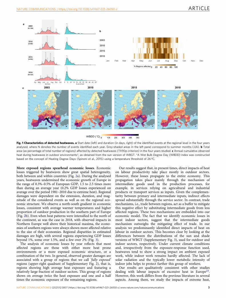
ResultsHeat spreads unevenly across Europe. Extreme hot spells inEurope varied greatly in frequency, duration, extension, andseverity in the years analysed (2003, 2010, 2015, and 2018).Considering the 274 regions contained in our area of study (seethe Methods for further details) and adopting the TX90p criter-ion, an average of N= 1180 (s.d.: ±230.2) regional heatwaveevents were identified per year. The temporal distribution patternof the emergence of heatwaves was multimodal, with peaksarising as a result of high-amplitude heat episodes (Fig. 1a, leftpanel). The case of 2010 is particularly illustrative, with a largeheatwave sweeping the continent at the end of June (Fig. 1a). Theduration of the median heatwave ranged from 5 to 6 days, with2003 and 2018 being the years showing events with higher meanduration (8.20 and 8.24 days, respectively; Fig. 1a, right panel).Years 2003 and 2018 featured the events with the longest duration(Fig. 1a), with a small fraction of heatwaves surpassing two weeks.Most heatwaves were concentrated during the summer months(June, July and August; JJA henceforth), but extended before andafter this time frame, particularly in 2003 and 2018 (Fig. 1a, b).However, heatwaves initiated during summer were on averagetwo times longer (8.5 versus 4.3 days) and more severe than non-summer heatwaves.

The total European area affected by heatwaves varies accordingto the time of the year analysed (Fig. 1b). The average heatwaveaffected 27–38% of the European territory, a situation thatbecomes aggravated during summer months, with an averagespatial extension of 49% of the total number of regions studiedand a maximum coverage of more than 95% during large-scaleepisodes. Years 2003 and 2018 showed events with higher spatialcoverage, with a summer average of around 55% of the totalEuropean area. From a regional perspective, heatwaves in 2003concentrated in central Europe, affecting mainly regions ofFrance, Germany, and Italy (Supplementary Table 1). Thesummer of 2010 showed less heat exposure in Western Europe,affecting primarily Eastern Europe and Russia29. SouthernEurope and the Baltic countries experienced more frequentheatwaves in 2015. In contrast, 2018 was exceptionally hot inregions where heatwaves are typically less frequent (see alsoWMO30). During that year, Northern Europe, in particularScandinavian countries, experienced sustained positive tempera-ture anomalies, which added up to around 2 calendar months.

It is important here to distinguish between the duration andthe severity of a heatwave. Both elements are relevant for thedetermination of productivity losses, but the latter is essential, asthe physiological effects of heat on workers usually emerge abovethe WBGT threshold of 26 °C31. To illustrate heatwave severity,we adapted the concept of heating degree-days of ref. 32, generallyused to calculate total energy demand. A Wet Bulb Degree-Day(WBDD) is here defined as any additional Wet-Bulb degree over26 °C experienced by a worker under heatwave days, consideringonly working hours. Total outdoor WBDD per year and regionare shown in Fig. 1c, reflecting that southern regions tend toalways suffer from high cumulative heat stress, even when heatpatterns become more intensified in other latitudes (see alsoSupplementary Fig. 1). Our analysis of regional heatwaves showsthat these events are largely heterogeneous in terms of spatial andtemporal characteristics (see, for example, Northern Italy in 2003or Croatia in 2003 and 2015 in Fig. 1c). This underpins theimportance of using local and timely data as well as high-resolution economic tools when it comes to analyse the impactsof heatwaves and other related extreme weather events.

ARTICLE NATURE COMMUNICATIONS | https://doi.org/10.1038/s41467-021-26050-z

2 NATURE COMMUNICATIONS | (2021) 12:5807 | https://doi.org/10.1038/s41467-021-26050-z | www.nature.com/naturecommunications

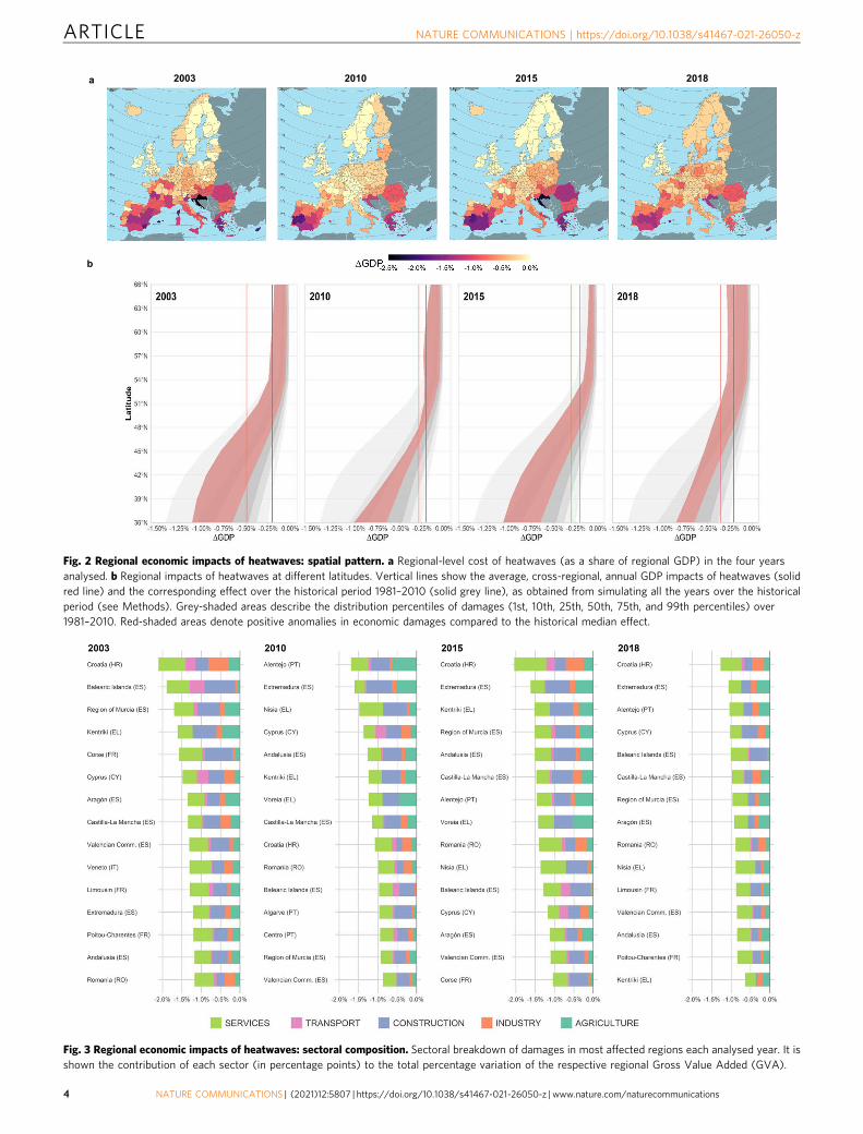
More exposed regions spearhead economic losses. Economiclosses triggered by heatwaves show great spatial heterogeneity,both between and within countries (Fig. 2a). During the analysedyears, heatwaves undermined the economic growth of Europe inthe range of 0.3%–0.5% of European GDP, 1.5 to 2.5 times morethan during an average year (0.2% GDP losses experienced onaverage over the period 1981–2010 due to extreme heat). Regionaldamages were dependent on the extension, duration, and mag-nitude of the considered events as well as on the regional eco-nomic structure. We observe a north-south gradient in economiclosses, consistent with average warmer temperatures and higherproportion of outdoor production in the southern part of Europe(Fig. 2b). Even when heat patterns were intensified to the north ofthe continent, as was the case in 2018, with observed impacts inNorthern Europe well above their historical maxima, the econo-mies of southern regions were always shown more affected relativeto the size of their economies. Regional disparities in estimateddamages are high, with several regions experiencing GDP lossesbeyond 1%, some over 1.5%, and a few over 2% (Fig. 3).

The analysis of economic losses by year reflects that mostaffected regions are those with either more heat proneenvironments or a more exposed economic structure, or acombination of the two. In general, observed greater damages areassociated with a group of regions that we call ‘fully exposed’regions (upper-right quadrant of Supplementary Fig. 2), that is,regions showing high average heat exposure and featuring arelatively large fraction of outdoor sectors. This group of regionsshows on average twice the heat exposure and one and a halftimes the economic exposure of the remaining regions.

Our results suggest that, in present times, direct impacts of heaton labour productivity take place mostly in outdoor sectors.However, these losses propagate to the entire economy. Thispropagation takes place mainly through the mechanism ofintermediate goods used in the production processes, forexample, in services relying on agricultural and industrialproducts or transport services as inputs. Given the complemen-tarity between primary and intermediate inputs, indirect effectsspread substantially through the service sector. In contrast, trademechanisms, i.e., trade between regions, act as a buffer to mitigatethis negative effect by substituting intermediate goods from lessaffected regions. These two mechanisms are embedded into oureconomic model. The fact that we identify economic losses inmost indoor sectors, suggest that the intermediate goodsmechanism outweighs the mitigating effect of trade. In ouranalysis we predominantly identified direct impacts of heat onlabour in outdoor sectors. This becomes clear by looking at thedifferences between the distributions of the sun and shadeversions of WBGT (Supplementary Fig. 3), used for outdoor andindoor sectors, respectively. Under current climate conditionsand, irrespectively from the exposure-response function used,heatwaves tend to show a strong impact on ambient exposedwork, while indoor work remains hardly affected. The lack ofsolar radiation and the typically lower metabolic intensity ofindoor jobs helps to protect further this group of workers.

Our results are qualitatively consistent with other studiesdealing with labour impacts of excessive heat in Europe23.However, this work differs from the previous literature in severalaspects. Among them, we study the impacts of extreme heat,

8102510201023002

a

b

c

Fig. 1 Characteristics of detected heatwaves. a Start date (left) and duration (in days, right) of the identified events at the regional level in the four yearsanalysed, where N denotes the number of events identified each year. Grey-shaded areas in the left panel correspond to summer months (JJA). b Totalarea (as percentage of total number of regions) affected by detected heatwaves (TX90p criterion) in the four years studied. c Annual cumulative observedheat during heatwaves in outdoor environments*, as obtained from the sun version of WBGT. *A Wet Bulb Degree Day (WBDD) index was constructedbased on the concept of Heating Degree Days (Spinoni et al., 2015) using a temperature threshold of 26 ºC.

NATURE COMMUNICATIONS | https://doi.org/10.1038/s41467-021-26050-z ARTICLE

NATURE COMMUNICATIONS | (2021) 12:5807 | https://doi.org/10.1038/s41467-021-26050-z | www.nature.com/naturecommunications 3

8102510201023002a

b

Fig. 2 Regional economic impacts of heatwaves: spatial pattern. a Regional-level cost of heatwaves (as a share of regional GDP) in the four yearsanalysed. b Regional impacts of heatwaves at different latitudes. Vertical lines show the average, cross-regional, annual GDP impacts of heatwaves (solidred line) and the corresponding effect over the historical period 1981–2010 (solid grey line), as obtained from simulating all the years over the historicalperiod (see Methods). Grey-shaded areas describe the distribution percentiles of damages (1st, 10th, 25th, 50th, 75th, and 99th percentiles) over1981–2010. Red-shaded areas denote positive anomalies in economic damages compared to the historical median effect.

Fig. 3 Regional economic impacts of heatwaves: sectoral composition. Sectoral breakdown of damages in most affected regions each analysed year. It isshown the contribution of each sector (in percentage points) to the total percentage variation of the respective regional Gross Value Added (GVA).

ARTICLE NATURE COMMUNICATIONS | https://doi.org/10.1038/s41467-021-26050-z

4 NATURE COMMUNICATIONS | (2021) 12:5807 | https://doi.org/10.1038/s41467-021-26050-z | www.nature.com/naturecommunications

understood as periods when a region’s temperatures areabnormally high (rather than measuring the effect of summeraverage temperatures), consider all the productive economicsectors, and adopt a higher spatio-temporal resolution level. Wealso tested the sensitivity of our findings to the choice of differentheat-exposure functions (see Methods, Heat exposure functions).Resulting differences responded to how different heat exposurefunctions were constructed and were proportional across thethree considered approaches, producing on average 11% lessdamages in the case of NIOSH and 30% in the case of Hothapscompared to ISO standards (Supplementary Fig. 4).

There are a number of reasons that lead us to think of thereported costs here only as a lower bound of the actual labour-related economic damages caused by heatwaves. First, our estimatesdo not include the costs caused by heat-derived occupationalinjuries33,34 and their related public health costs. Second, thecalibration of the heat exposure functions is based on a fewempirical studies, where production subsectors are treated homo-geneously, thus not capturing well their workload diversity. On theopposite side, this study does not consider the likely existence ofadaptation and heat-insulation measures adopted by companies andhouseholds, such as air conditioning, extensively implemented inEurope35. However, since the implementation of heat-insulationmeasures is still quite low in outdoor sectors and air conditioningavailability only affects indoor sectors, these adaptation effects dolikely not have a significant impact on our current estimates.

Projected costs under unmitigated scenarios. Our approach tofuture climate scenarios focuses on a 30-year period spanned by

the years 2035–2064, for which the number and severity ofregional heatwaves were calculated. Climate model projectionsare subject to large uncertainties regarding the model, initialconditions or emission scenario considered36,37. We sought toaccount for these uncertainties by analysing two different climatemodels, which are representative simulations of different warm-ing conditions over Europe (see Methods) selected from a largermulti-model ensemble5, and by focusing on a 30-year period bymid-century, less affected by the chosen emission scenario. In thetwo considered models, we observed an increase in heat severityfor both outdoor and indoor workers5. In contrast to what isobserved during current heatwaves, our projections of WBGTsuggest that indoor workers will become more directly affected byheat, especially in regions from southern and central Europe,provided current working conditions and insulation methodsprevail (Supplementary Fig. 3, see the projected shift in theWBGT distribution in red).

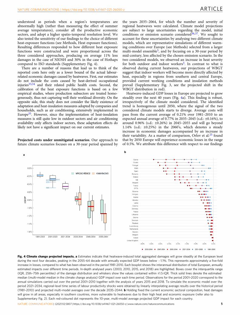
Heatwave-induced GDP losses in Europe are projected to growsteadily over the next 40 years (Fig. 4a). This finding is robust,irrespectively of the climate model considered. The identifiedtrend is homogenous until 2050, where the signal of the twoconsidered climate models starts to diverge. Average costs willpass from the current average of 0.21% over 1981–2010 to anexpected annual average of 0.77% in 2035–2045 (s.d.: ±0.16%), toaround 0.96% (s.d.: ±0.26%) in 2045–2055 and will go beyond1.14% (s.d.: ±0.25%) in the 2060’s, which denotes a steadyincrease in economic damages accompanied by an increase intheir variability. As a matter of comparison, Orlov et al.25 foundthat by 2050 Europe will experience economic losses in the rangeof 0.5%. We attribute this difference with respect to our findings

Fig. 4 Climate change projected impacts. a Estimates indicate that heatwave-induced total aggregated damages will grow steadily at the European levelduring the next four decades, peaking in the 2055–64 decade with annually expected GDP losses below −1.1%. This represents approximately a five-foldincrease in losses, compared to what has been observed in the period 1981-2010. Each boxplot shows the interannual distribution of total European, annuallyestimated impacts over different time periods. In-depth analysed years (2003, 2010, 2015, and 2018) are highlighted. Boxes cover the interquartile range(IQR, 25th–75th percentiles) of the damage distribution and whiskers show the values contained within ±1.5⋅IQR. Thick solid lines denote the estimatedmedian (multi-model median in the climate change analysis) GDP impact over each time period. Observations for the period 2001–2020 correspond to theannual simulations carried out over the period 2001–2010 together with the analysis of years 2015 and 2018. To simulate the economic model over theperiod 2021–2034, regional-level time series of labour productivity shocks were obtained by linearly interpolating average results over the historical period(1981–2010) and projected multi-model averages over the decade 2035–2044. b Holding fixed the current economic sectoral composition, heat damageswill grow in all areas, especially in southern countries, more vulnerable to heatwaves due to their high heat and economic exposure (refer also toSupplementary Fig. 2). Each red-coloured dot represents the 10-year, multi-model average projected GDP impact for each country.

NATURE COMMUNICATIONS | https://doi.org/10.1038/s41467-021-26050-z ARTICLE

NATURE COMMUNICATIONS | (2021) 12:5807 | https://doi.org/10.1038/s41467-021-26050-z | www.nature.com/naturecommunications 5

mainly to the heat-exposure function used (Hothaps in ref. 25;ISO in this study), as ISO is more sensitive to lower temperatures(Supplementary Fig. 3; Supplementary Fig. 4) as well as todifferences in the parametrisation of the economic model and theexperimental design, as the cited work is based on a dynamicframework. Carefully exploring different climate and socio-economic (RCP-SSP) combinations is vital to assess theuncertainty posed by future projected scenarios to the presentresults (the reader is referred to the Supplementary Discussion foran overview of the projected outcomes under the scenarioRCP8.5-SSP5).

Aggregating our regional estimates at the country level, wefound that southern European countries will clearly be the mosteconomically harmed by excessive heat in the future (Fig. 4b).Aside from Cyprus, the country with current and future highestrelative losses, we identified that Portugal, Spain, and Croatia willgradually move from a range of losses of 2% in 2040 to around 3%in 2060. As it happens in present times, large heterogeneities inimpacts are also expected within countries in this area, due todifferent regional heat and economic exposure (SupplementaryFig. 5). Balkan countries, Italy, and Greece will also experienceconsiderable increases in their expected damages, with averageannual losses of more than 2% in 2055–2064 attributed to extremeheat. Central and northern European countries will experienceminor but significant negative impacts (p-value < 0.001), asthermal stress will increase across all latitudes. GDP impacts inthose regions will be more modest but still meaningful, withGermany being projected to experience a negative impact on GDPof 0.5% by 2050, similar to what is reported in Knittel et al.24, whoalso include the productivity effects of non-EU imports in theirestimates. In contrast, UK, Iceland and Scandinavian countrieswill only suffer very mild losses, ranging from 0% to 0.2% of GDP.

The climate change signal provided by these two and otherclimate models for the next four decades is very similar,irrespectively of the emission scenario considered (see ref. 5 forthe full ensemble of simulations; scenarios depict more distinctsignals from 2050 onwards). Hence, heatwave-related productiv-ity losses are expected to increase considerably in Europe by themid-21st century even if stringent mitigation pathways wereadopted. There exist, however, big margins for adaptation andacclimatisation, even though adapting to low-probability extremeevents could challenge our potential adaptability38.

DiscussionAt the European level, total annual losses attributable to heat-waves amounted to 0.3–0.5% of European GDP in the analysedyears (2003, 2010, 2015, and 2018) while the average GDP lossover the period 1981–2010 was estimated to be close to 0.2%.Nevertheless, southern regions were consistently shown morevulnerable to these damages due to their high geographical andeconomic exposure to heat, experiencing GDP losses above 1%and, occasionally, above 2%. Under current climate conditions,outdoor workers seem disproportionately more affected byextreme heat, while most indoor work remains insulated. Theanalysis of the distribution of our heat stress measures (WBGTsun

and WBGTshade) suggests the presence of generalised and wide-spread outdoor productivity impacts but very mild indoor pro-ductivity damages only in southernmost regions. However,economic damages in outdoor activities spread to the remainingsectors due to the tight interconnectedness of the economic sys-tem. For example, sectors dependent on agricultural inputs, suchas food manufacturing, tourism, and travel-related services, wereshown largely affected. Meanwhile, bilateral trade betweenregions and input factor substitutability between sectors acted assmoothing factors to total damages. Looking ahead, the projected

costs of heatwaves are expected to increase steadily in the nextdecades if no further measures to adapt to warmer temperaturesare implemented in work environments. Economic losses areprojected to increase by almost a factor of five by 2060 comparedto the historical damages experienced over the period 1981–2010and will affect more the areas where heatwave-induced pro-ductivity damages are already pronounced.

We recognise the existence of additional factors that can play arole in a comprehensive assessment of the costs associated withexcessive heat in work environments. First, heat-induced occu-pational injuries temporally shrink the effective labour force,harming total production while increasing public health costs.Occupational injuries data availability at the regional level, cur-rently very limited, must be guaranteed for an effective integra-tion of this dimension into our analysis. Second, the incrementalheat effect in urban areas (see39 and references therein), i.e., theurban heat island effect, and its potential large effects on, forexample, construction workers, should be explored with theWBGT or alternative heat stress indicators including a humanheat balance model, such as the Mean Radiant Temperature(MRT) and the Universal Thermal Climate Index (UTCI)40,always adopting enough spatial resolution and/or parameterisedprocesses to capture heat signals at the city level. Third, thepresence of adaptation measures, such as air conditioning, maylessen heat-derived economic damages41. Its unlikely imple-mentation in outdoor environments and the current absence ofdirect heat effects on indoor activities do likely not compromiseour current estimates but can potentially affect our climatechange results. Fourth, we used the existing state-of-the-artfunctions to translate heat stress into labour productivity impacts.Emerging field studies are beginning to provide evidence on theexistence of heat stress impacts on productivity at temperaturesbelow 26 °C WBGT2,42,43, also featuring notable disparitieswithin economic sub-sectors. Nevertheless, the results from thesefield studies have yet to be translated into more sophisticated,sector-specific transfer functions. Fifth, a comprehensive assess-ment based on the combination of future climate and socio-economic pathways must be carried out in order to obtain acomplete overview of the distribution of future heatwave impactsand their associated uncertainties. However, for this kind ofassessment, hourly-level and spatially downscaled projections ofheat stress measures should first be available under differentclimate forcings and existing regional SSP narratives need to beable to accommodate changes in the regional economicstructure44. These five gaps should be addressed by futureresearch.

Beyond measuring the economic damages triggered by extremeheat, the proposed methodology can also be used as a tool for theassessment of future occupational health and the formulation oflocal-level adaptation policies. Finally, this study reinforces theneed for spatially resolved, bottom-up approaches as a requisiteto capture local socio-economic and climatic idiosyncrasies,crucial to analyse the potential economic consequences of climatechange.

MethodsArea of study. 274 regions representing all the EU-27 countries, United Kingdomand EFTA countries (Iceland, Norway, and Switzerland) were considered. Whereavailable (EU-27 and UK), we adopted the second-level Nomenclature of Terri-torial Units for Statistics (NUTS 2) classification as the administrative basic unit ofreference. Before feeding the model with the respective labour productivity shocks,a subsequent spatial aggregation procedure was required for some regions, sincethe resolution of the economic model was not the same for all countries because ofthe difficulty to estimate mutually consistent regional-level Social AccountingMatrices (SAMs) required to calibrate the economic model (refer to SupplementaryTable 2 for a description of the spatial resolution used in the economic model).Typically, higher spatial disaggregation levels (NUTS 2) were available for moreeconomically relevant countries (France, Italy, and Spain). NUTS 0 (country) or

ARTICLE NATURE COMMUNICATIONS | https://doi.org/10.1038/s41467-021-26050-z

6 NATURE COMMUNICATIONS | (2021) 12:5807 | https://doi.org/10.1038/s41467-021-26050-z | www.nature.com/naturecommunications

NUTS 1 (sub-country) population-weighted spatial aggregation was applied toobtain the values in the remaining regions.

Heatwaves characterisation. There is no consistent and methodical approach todefining heatwaves (sometimes also referred to as warm spells)45,46. For example,the Intergovernmental Panel on Climate Change defines a heatwave as ‘a period ofabnormally hot weather’. Furthermore, several criteria have been used to char-acterise heatwaves based on mean, maximum, minimum temperature, humidity, ora combination of those47. In this study, we selected the TX90p criterion, i.e., aheatwave occurs when the 90th percentile of maximum temperatures is exceededfor at least 3 consecutive days. This criterion is based on the anomaly of maximumtemperature and includes information about the entire annual cycle, which easesthe identification of productivity impacts above a certain threshold of temperature.Using the period 1981–2010 as the reference to calculate temperature percentiles,we identified the number of heatwaves taking place in four years consideredanomalously hot in Europe29,48–50, namely 2003, 2010, 2015, and 2018, andaccounted for the duration, severity and spatial scope of these events.

Heat stress index. The Wet Bulb Globe Temperature (WBGT) was used as a heatstress index. WBGT is the most widely used index to determine heat stress in anoccupational context (e.g., 23,51–53), it can be easily obtained from standardmeteorological variables and is recommend by the International Standard Orga-nization as occupational heat stress index54. WBGT was calculated using the Rpackage HeatStress55 for both outdoor, i.e., WBGT in the sun (WBGTsun), andindoor environments, i.e., WBGT in the shade (WBGTshade). WBGTsun

56 takes intoaccount air temperature, dew point temperature, wind speed, and solar radiation,whereas WBGTshade is a simplified version based on air temperature and dew pointtemperature only57, assuming a wind speed of 1 m/s (slow walk). For detailedinformation on the WBGT calculations and their formulations, the reader isreferred to Lemke and Kjellstrom58. Hourly WBGT values were used to calculatethe respective productivity losses due to heat exposure during working time. Theuse of hourly WBGT is essential to capture intra-daily heat variability, since theheat stress level encompasses the actual time devoted to work, avoiding the pre-sence of potential biases resulting from the use of 24 h, day- or night-time tem-perature (e.g. 5, illustrate the clear underestimation of heat stress based on dailymean WBGT).

Measures to mitigate excessive heat include rescheduling tasks, increasing thenumber of breaks, or switching activities from outdoor to indoor environments.Although it is true that in some occupational settings the productivity lossestriggered by excessive heat or the working time loss related to more frequent breaksmay be reduced by rescheduling certain tasks59, some of these countermeasures arealready implemented in normal or warm days (and, therefore, workers cannotfurther change their behaviour during a heatwave) while other tasks need to becompleted at specific hours of the day or location. Also, benefits from switchingactivities from sun to shadow are sometimes outweighed by aggravated effects ofdirect sunlight exposure60. Thus, the inherent flexibility of the WBGT, whichallows to account for heat stress for either indoors or outdoors with a single index,entail an important advantage.

Climate data. For the analysis of past heatwave events, we used ERA5-Landreanalysis data61, which provides hourly estimates of a large number of atmo-spheric climate variables on a high-resolution grid (0.1° × 0.1°; native resolution is9 km). Daily maximum temperature from 1981 to present was used to account forpast heatwaves. Heatwaves were identified at the regional level using the TX90pcriterion, i.e., when the 90th percentile of the distribution of regional maximumtemperatures spanned by data from the period 1981–2010 was exceeded for at least3 consecutive days. Additionally, hourly values of near surface air temperature, dewpoint temperature, solar radiation, and wind speed data for the four selected yearswere retrieved to obtain hourly values of WBGT (see section above).

In the climate change exercise, we studied a period by mid-21st century(2035–2064), which is a compromise between using a not too distant future forimmediate action and far enough so that the climate change signal emerges fromthe internal natural climate variability62. We assessed the evolution of heat stresscosts based on two different climate model projections stemming from regionalclimate model (RCM) simulations from EURO-CORDEX63,64 and griddedobservational data (WFDEI, WATCH Forcing Data methodology applied to ERA-Interim data65), where the latter was necessary to establish the correction ofsystematic biases in the climate model data. For this purpose, we applied theempirical quantile mapping technique (QM66), using the implementation fromRajczak et al.67. QM was calibrated between the daily observed and modelleddistributions of the input variables of the WBGT in the period 1981–2010 prior tothe index calculation, resulting in bias-corrected projections of daily WBGT on a0.5° grid (approximately 50 km). More methodological details and a comprehensiveevaluation of the bias-corrected WBGT (in particular, the multivariate structure) ispresented in Casanueva et al.68. Heatwaves over this period were estimated takingthe historical period 1981–2010 as reference69.

We focused on projections based on the emission scenario RCP8.5, asdifferences between the various scenarios were found to be small within theconsidered time horizon. In particular, we considered two specific simulations

which were chosen among a large ensemble of RCM simulations5, namely,MPICSC-REMO2 driven by MPIESM (RCP8.5, EUR-44) and KNMI-RACMOdriven by HADGEM (RCP8.5, EUR-11). They are representative simulations of thelower and the upper 25% of the distribution of climate change signals of summermean temperature averaged across Europe in the period 2070–20995,70.

Hourly future values of WBGT were approximated from daily mean andmaximum WBGT values based on the 4+ 4+ 4 approach5,51. Note that dailymean WBGT values were calculated from daily mean values of the consideredinput variables, whereas daily maximum WBGT values were estimated with dailymaximum air temperature and solar radiation, and daily mean dew pointtemperature and wind speed. The 4+ 4+ 4 method assumes the daily maximumWBGT value during the hottest part of the day (12–16 h), the daily mean WBGTduring 2 h in the early morning (8–10 h) and 2 h in the early evening (18–20 h),and the average of daily mean and daily maximum WBGT values during theremaining 4 h (10–12 h and 16–18 h).

Heat exposure functions. Heat stress experienced in different environments andmetabolic loads were transformed into productivity losses using the ISO, NIOSH,and Hothaps heat exposure metrics31. The sun and shade versions of the WBGTwere considered for outdoor and indoor activities, respectively. Economic sectorswere classified into three different categories depending on their workload intensity(Supplementary Table 3). Low, moderate, and high workload groups were identi-fied. Hourly work ability (workability) levels were computed and expressed in therange of 0–100%, where 100% represents no productivity damages and 0% denotesinability to work. Workability hourly values for the ISO and NIOSH approacheswere obtained as

workabilityðISO;NIOSHÞ;h ¼ max 0;min 1;WBGTlim;rest WBGTh

WBGTlim;rest WBGTlim

!" #( )ð1Þ

where h denotes the hour of day, WBGTlim;ISO ¼ 34:9M=46 andWBGTlim;NIOSH ¼ 56:7 11:5log10M. WBGTlim;rest results from applying Eq. 1 tothe resting metabolic rate Mrest ¼ 117W54. Selected values of M for low, medium,and high workloads were M ¼ f200; 300; 400gW, respectively.

Contrary to the workability estimates based on WBGTlim, showing a lower limitof 0% (Eq. 1), the Hothaps approach71 proposes a lower limit of 10%, i.e., workingis possible for 6 min. within each hour even under extreme heat. Hothapsworkability values were approximated with the following two-parameter logisticfunction

workabilityHothaps ¼ 0:1þ 0:9=½1þ ðWBGT=α1Þα2 ð2Þ

where the set of parameters ðα1; α2Þ were equal to (34.64, 22.72) for low, (32.93,17.81) for moderate and (30.94, 16.64) for high workload, respectively. However,the Hothaps functions are subject to great parameter uncertainty due to beingbased on a few empirical studies. Therefore, we adopted the ISO standards as ourbenchmark functions and used the NIOSH and Hothaps functions to test for thesensitivity of our estimates.

A constant and homogenous working day was assumed to take place from 9 hto 17 h. Hourly workability values were averaged at the daily level for all days in aheatwave.

Population data. An effort was made to situate economic activity. Gridded data onheat-induced worker productivity losses were matched with population masks toobtain population-weighted impacts on worker productivity. We used the griddedUN WPP-adjusted population count data v4.11, provided by the SocioeconomicData and Applications Center (SEDAC, Columbia University; CIESIN Center forInternational Earth Science Information Network72). Since only data for years2000, 2005, 2010, 2015, 2020 were available, year-specific population masks werecalculated by linear interpolation. The spatial mismatch between the resolution ofpopulation (0.25°) and climate data (0.1° for the reanalysis and 0.5° for the bias-corrected climate model data) were handled by interpolating the latter towards thepopulation grid using the nearest neighbour. In the climate change analysis, weretrieved population data (0.25° resolution) for the years 2030, 2040, 2050, 2060,and 2070 under the scenario SSP573,74, denoting a situation of high energy andresource intensity based on fossil fuel development, consistent with the emissionscenario RCP8.5. The same procedure of temporal interpolation of the populationdata and spatial interpolation of the climate data towards the population grid wasapplied.

Accounting for seasonal patterns in economic activity. Seasonal and calendareffects matter if an accurate economic measurement is sought. For example,heatwaves tend to concentrate during summer months while economic outputgenerated by outdoor activities, such as agricultural work, is also predominantduring that time of the year. We controlled for seasonality by weighting all theeconomic shocks by the number of heatwave days per quarter. We used economicdata from the Quarterly National Accounts provided by Eurostat75 to approximatethe seasonal pattern of regional-sectoral activities.

NATURE COMMUNICATIONS | https://doi.org/10.1038/s41467-021-26050-z ARTICLE

NATURE COMMUNICATIONS | (2021) 12:5807 | https://doi.org/10.1038/s41467-021-26050-z | www.nature.com/naturecommunications 7

Regional computable general equilibrium (CGE) model. The sub-national CGEmodel used is based on the GTAP model76 and was calibrated on the GTAP 8database and parameters for the reference year 200777. The choice of the calibra-tion year might bias to some extent the outcome of our simulations, as the regionaldatabase already incorporates the effect of heatwaves in the economy during thecalibration year. We expect, however, this bias to be low in our case, as 2007 was ingeneral a lower-than-average year in terms of heat load.

The GTAP database is a series of Social Accounting Matrices (SAMs) for 129countries or groups of countries and 57 sectors covering the global economy. Themaximum level of spatial detail in GTAP is the country level. For this reason, wecomplemented the GTAP database with regional economic information retrievedfrom Eurostat and countries’ National Statistical Offices. We also followed amethodology based on Simple Location Quotients (SLQs) and gravity equations toget mutually consistent regional SAMs and bilateral trade flows between the EUsub-country regions26.

The model follows the neoclassical paradigm, where investments are saving-driven and primary factors (labour and capital) are fully employed. Morespecifically, labour and capital can move between different economic sectors butnot outside the region in which they are located. Production is represented by aLeontief technology between factors of production and value added, which is inturn a Constant Elasticity of Substitution (CES) function between the primaryfactors. When a shock hits the economic system, agents (households and firms)adjust their economic decisions (consumption, production, primary factorsallocation) based on relative price changes.

One relevant feature of our sub-national version of the GTAP model concernsthe specification of the trade relationships between regions. In CGE modelling,including the GTAP framework, the Armington assumption is typically used tomodel the trade structure. Armington elasticities imply an imperfect substitutionbetween domestic and foreign products, which prevents an unrealistic sectoralspecialisation after a shock being absorbed by the model. We developed the tradestructure of the GTAP model regionally to disentangle the international and intra-national trade flows. Unlike the standard GTAP country-level specification, weinclude the domestic sub-national demand and the intra-national imports fromother regions. We used two types of functions to model our trade structure. TheCES function links the sub-national domestic demand and the aggregate imports ofthe sub-national region and uses an elasticity of substitution σARM between the twovariables. The CRESH (Constant Ratios of Elasticity of Substitution, Homothetic78)function breaks the aggregate imports according to the source region, which can bea region within or outside the country. In this case, the elasticity is the bi-dimensional σIMP , which allows us to identify the source and the destination regionand to differentiate between intra- and international trade. Compared to thestandard GTAP model, we increase σIMP by 20% if the region is trading withanother region within the country. This calibration is based on the so-called bordereffect79, which states that, ceteris paribus, trade between two locations is reduced by20-50% if these two locations are separated by national borders80. We adopt aconservative choice on the value of Armington elasticities for sub-national unitsbecause we focus on the short-term economic consequences of heatwaves, whentrade frictions can be high. This value is meant to provide only a reference to maketrade more fluid within a country than between countries. Further research and asensitivity analysis on this value would be certainly valuable but is out the scope ofthe paper.

Regional Value Added (VA) for region r and sector s is represented in the CGEmodel with a constant return to scale function of capital and labour as follows:

VArs ¼ χrsKσs1σsrs ψrsL

σs1σsrs

σs1σs ð3Þ

where the total value added generated by region r in sector s in a certain yeardepends on the combined use of capital (K) and labour (L), each of which show aspecific degree of region-sector factor productivity, χ and ψ, respectively. Theparameter σS denotes the elasticity of substitution between primary factors.

Coupling between biophysical impacts of heat and economic model. Since theeconomic model shows a yearly temporal resolution, we transformed all the pro-ductivity shocks to their annual equivalents before simulating the model. During agiven year, the productivity of labour in region r and sector s was assumed to bereduced by a percentage τrs , that is,

ψ0rs ¼ ð1 τrsÞψrs ð4Þ

where the parameter τ represents the annual-equivalent average workability inregion r and sector s. We calculated τ for each region-sector combination at each ofthe analysed years using MS Excel.

Historical GDP losses. For the sake of comparison, the distribution of historicaleconomic losses in response to heatwaves was calculated for the period 1981–2010.Using historical maximum temperature records, regional heatwaves were identifiedalong the whole reference period and their severity was documented. Regional-level, sun and shade WBGT values were calculated after retrieving the full timeseries of WBGT components from the ERA5-Land hourly data catalogue over theperiod 1981–2010. Since CIESIN population count data was not available for the

period 1981–1999, we used population data from year 2000 as weighting factor.The resulting WBGT values were used to obtain the respective regional-sectoralannual productivity losses and shocks, which were used to hit the economic modelas described in the section above to derive the underlying regional economic losses.

Reporting summary. Further information on research design is available in the NatureResearch Reporting Summary linked to this article.

Data availabilityThe historical climate data that support the findings of this study are publicly available atthe Copernicus Climate Data Store (https://doi.org/10.24381/cds.bd0915c6). Futureclimate projections are available for download via the Earth System Grid Federation(ESGF, https://esgf.llnl.gov/) under the project name “CORDEX” at any of the ESGFnodes, such as for example, https://esgf-node.ipsl.upmc.fr/search/cordex-ipsl/. The SocialAccounting Matrices (GTAP) used to calibrate the economic model were used underlicense for the current study, and so are not publicly available. Data are however availablefrom the authors upon reasonable request and with permission of the Center for GlobalTrade Analysis, Department of Agricultural Economics, Purdue University. UN WPP-Adjusted Population Count, v4.11 are available for download at https://sedac.ciesin.columbia.edu/data/set/gpw-v4-population-count-adjusted-to-2015-unwpp-country-totals-rev11. Quarterly sectoral accounts used in the seasonal adjustment ofproductivity shocks were obtained from Eurostat (https://ec.europa.eu/eurostat/databrowser/view/namq_10_gdp/default/table?lang=en).

Code availabilityThe two versions of the WBGT used in this study were implemented in R using the Rpackage HeatStress (https://github.com/anacv/HeatStress. https://doi.org/10.5281/zenodo.3264929), under license GPL-3.

Received: 17 April 2020; Accepted: 1 September 2021;

References1. Dunne, J. P., Stouffer, R. J. & John, J. G. Reductions in labour capacity

from heat stress under climate warming. Nat. Clim. Change 3, 563–566(2013).

2. Flouris, A. D. et al. Workers’ health and productivity under occupational heatstrain: a systematic review and meta-analysis. Lancet Planet. Health 2,521–531 (2018).

3. Graff-Zivin, J. S. & Neidell, M. J. Temperature and the allocation of time:implications for climate change. J. Labor Econ. 32, 1–26 (2014).

4. Heal, G. & Park, R. J. Temperature stress and the direct impact of climatechange: a review of an emerging literature. Rev. Environ. Econ. Policy 10,347–362 (2016).

5. Casanueva, A. et al. Escalating environmental summer heat exposure - a futurethreat for the European workforce. Regional Environ. Change 20, 1–14 (2020).

6. Ioannou, L. G. et al. Effect of a simulated heat wave on physiological strainand labour productivity. Int J. Environ. Res Public Health 18, 3011 (2021).

7. Takakura, J., Fujimori, S. & Takahashi, K. et al. Cost of preventing workplaceheat-related illness through worker breaks and the benefit of climate-changemitigation. Environ. Res. Lett. 12, 064010 (2017).

8. Park, R. J., Goodman, J., Hurwitz, M. & Smith, J. Heat and learning. Am. Econ.J. Econ. Policy 12, 306–339 (2020).

9. Heyes, A. & Saberian, S. Temperature and decisions: evidence from 207,000court cases. Am. Econ. J. Appl. Econ. 11, 238–265 (2019).

10. Harrington, L. J. & Otto, F. E. L. Reconciling theory with the reality of Africanheatwaves. Nat. Clim. Change 10, 796–798 (2020).

11. EEA, European Environment Agency. Indicator Assessment. Global andEuropean temperatures. https://www.eea.europa.eu/data-and-maps/indicators/global-and-european-temperature-8/assessment. Accessed: 2020-09-10.

12. Diffenbaugh, N. S. Verification of extreme event attribution: using out-of-sample observations to assess changes in probabilities of unprecedentedevents. Sci. Adv. 6, eaay2368 (2020).

13. King, A. D. et al. Emergence of heat extremes attributable to anthropogenicinfluences. Geophys. Res. Lett. 43, 3438–3443 (2016).

14. Perkins-Kirkpatrick, S. E. & Lewis, S. C. Increasing trends in regionalheatwaves. Nat. Commun. 11, 3357 (2020).

15. Stott, P., Stone, D. & Allen, M. Human contribution to the European heatwaveof 2003. Nature 432, 610–614 (2004).

16. IPCC. Climate change 2013: the physical science basis. Contribution ofworking group I to the fifth assessment report of the intergovernmental panelon climate change. In (eds. Stocker T. F., Qin D., Plattner G.-K., Tignor M.,Allen S. K., Boschung J., Nauels A., Xia Y., Bex V., Midgley P. M.) 1535(Cambridge University Press, Cambridge and New York, 2013).

ARTICLE NATURE COMMUNICATIONS | https://doi.org/10.1038/s41467-021-26050-z

8 NATURE COMMUNICATIONS | (2021) 12:5807 | https://doi.org/10.1038/s41467-021-26050-z | www.nature.com/naturecommunications

17. Fischer, E. M. & Schär, C. Consistent geographical patterns of changes inhigh-impact European heatwaves. Nat. Geosci. 3, 398–403 (2010).

18. Russo, S. et al. Magnitude of extreme heat waves in present climate and theirprojection in a warming world. J. Geophys. Res. Atmospheres 119,12500–12512 (2014).

19. Watts, N. et al. The 2019 report of The Lancet Countdown on health andclimate change: ensuring that the health of a child born today is not defined bya changing climate. Lancet 394, 1836–1878 (2019).

20. Císcar, J. C. et al. Climate impacts in Europe: Final report of the JRC PESETAIII project, (Publications Office of the European Union), JRC Science forPolicy Report EUR 29427 EN (2018).

21. Conway, D. et al. The need for bottom-up assessments of climate risks andadaptation in climate-sensitive regions. Nat. Clim. Change 9, 503–511 (2019).

22. García-León, D., Standardi, G. & Staccione, A. An integrated approach for theestimation of agricultural drought costs. Land Use Policy 100, 104923 (2021).

23. Orlov, A., Sillmann, J., Aaheim, A., Aunan, K. & de Bruin, K. Economic lossesof heat-induced reductions in outdoor worker productivity: a case study ofEurope. Econ. Disasters Clim. Change 3, 191–211 (2019).

24. Knittel, N., Jury, M. W., Bednar-Friedl, B., Bachner, G. & Steiner, A. K. Aglobal analysis of heat-related labour productivity losses under climate change—implications for Germany’s foreign trade. Climatic Change 160, 251–269(2020).

25. Orlov, A., Sillman, J., Aunan, K., Kjellstrom, T. & Aaheim, A. Economic costsof heat-induced reductions in worker productivity due to global warming.Glob. Environ. Change 63, 102087 (2020).

26. Bosello, F. & Standardi, G. The new generation of computable generalequilibrium models. (eds. Perali F., Scandizzo L. P.) 249–277 (Springer, 2018).

27. Giorgi, F. Uncertainties in climate change projections, from the global to theregional scale. EPJ Web Conf. 9, 115–129 (2010).

28. Hawkins, E. & Sutton, R. The potential to narrow uncertainty in regionalclimate predictions. Bull. Am. Meteorol. Soc. 90, 1095–1108 (2009).

29. Barriopedro, D., Fischer, E. M., Luterbacher, J., Trigo, R. M. & García-Herrera,R. The hot summer of 2010: redrawing the temperature record map of Europe.Science 332, 220–224 (2011).

30. World Meteorological Organization (WMO). WMO Statement on the State ofthe Global Climate in 2018. (WMO-No. 1233). Geneva (2019).

31. Bröde, P., Fiala, D., Lemke, B. & Kjellstrom, T. Estimated work ability in warmoutdoor environments depends on the chosen heat stress assessment metric.Int. J. Biometeorol. 62, 331–345 (2018).

32. Spinoni, J., Vogt, J. & Barbosa, P. European degree-day climatologies andtrends for the period 1951–2011. Int. J. Climatol. 35, 25–36 (2015).

33. Marinaccio, A. et al. Nationwide epidemiological study for estimating theeffect of extreme outdoor temperature on occupational injuries in Italy.Environ. Int. 133, 105176 (2019).

34. Martínez-Solanas, É. et al. Evaluation of the impact of ambient temperatureson occupational injuries in Spain. Environ. Health Perspect. 126, 067002(2018).

35. de Cian, E., Pavanello, F., Randazzo, T., Mistry, M. N. & Davide, M.Households’ adaptation in a warming climate. Air conditioning and thermalinsulation choices. Environ. Sci. Policy 100, 136–157 (2019).

36. Knutti, R. Should we believe model predictions of future climate change?Philos. Trans. R. Soc. Ser. A 366, 4647–4664 (2008).

37. Knutti, R. & Sedláček, J. Robustness and uncertainties in the new CMIP5climate model projections. Nat. Clim. Change 3, 369–373 (2013).

38. Suárez-Gutiérrez, L., Müller, W. A., Li, C. & Marotzke, J. Hotspots of extremeheat under global warming. Clim. Dyn. 55, 429–447 (2020).

39. Burgstall A. Representing the urban heat island effect in future climates. MScThesis, University of Augsburg. Available at https://www.meteoschweiz.admin.ch/home/service-und-publikationen/publikationen.subpage.html/de/data/publications/2020/2/representing-the-urban-heat-island-effect-in-future-climates.html (2019).

40. Di Napoli, C., Barnard, C., Prudhomme, C., Cloke, H. L. & Pappenberger, F.ERA5-HEAT: A global gridded historical dataset of human thermal comfortindices from climate reanalysis. Geosci. Data J. 00, 1–9 (2020).

41. Morris, N. B. et al. Sustainable solutions to mitigate occupational heat strain –an umbrella review of physiological effects and global health perspectives.Environ. Health 19, 95 (2020).

42. Ioannou, L. G. et al. Time-motion analysis as a novel approach for evaluatingthe impact of environmental heat exposure on labor loss in agricultureworkers. Temperature 4, 330–340 (2017).

43. Quiller, G. et al. Heat exposure and productivity in orchards: Implications forclimate change research. Arch. Environ. Occup. Health 72, 313–316 (2017).

44. Kok, K., Pedde, S., Gramberger, M., Harrison, P. A. & Holman, I. P. NewEuropean socio-economic scenarios for climate change research:operationalising concepts to extend the shared socio-economic pathways.Regional Environ. Change 19, 643–654 (2019).

45. IPCC. Glossary of terms. In: Managing the Risks of Extreme Events andDisasters to Advance Climate Change Adaptation (eds. Field, C. B., V. Barros,

T. F. Stocker, D. Qin, D. J. Dokken, K. L. Ebi, M. D. Mastrandrea, K. J. Mach,G.-K. Plattner, S. K. Allen, M. Tignor, and P. M. Midgley) 555–564 (A SpecialReport of Working Groups I and II of the Intergovernmental Panel onClimate Change (IPCC), Cambridge University Press, Cambridge, UK, andNew York, NY, USA, 2012).

46. World Meteorological Organization (WMO). International meteorologicalvocabulary. Second edition. (WMO-No. 182). Geneva (1992).

47. Perkins, S. E. & Alexander, L. V. On the measurement of heat waves. J. Clim.26, 4500–4517 (2013).

48. Russo, S., Sillmann, J. & Fischer, E. M. Top ten European heatwaves since1950 and their occurrence in the coming decades. Environ. Res. Lett. 10,124003 (2015).

49. Schär, C. et al. The role of increasing temperature variability in Europeansummer heatwaves. Nature 22, 332–336 (2004).

50. Vogel, M. M., Zscheischler, J., Wartenburger, R., Dee, D. & Seneviratne, S. I.Concurrent 2018 Hot Extremes Across Northern Hemisphere Due to Human-Induced Climate Change. Earth’s Future 7, 692–703 (2019).

51. Kjellstrom, T., Freyberg, C., Lemke, B., Otto, M. & Briggs, D. Estimatingpopulation heat exposure and impacts on working people in conjunction withclimate change. Int. J. Biometeorol. 162, 291–306 (2018).

52. Chavaillaz, Y. et al. Exposure to excessive heat and impacts on labourproductivity linked to cumulative CO2 emissions. Sci. Rep. 9 (2019).

53. Li, D., Yuan, J. & Kopp, R. E. Escalating global exposure to compound heat-humidity extremes with warming. Environ. Res. Lett. 15, 064003 (2020).

54. ISO 7243:2017. Ergonomics of the thermal environment - Assessment of heatstress using the WBGT (wet bulb globe temperature) index. InternationalOrganisation for Standardisation, Geneva (2017).

55. Casanueva, A. HeatStress, Zenodo, https://doi.org/10.5281/zenodo.3264930(2019a).

56. Liljegren, J. C., Carhart, R. A., Lawday, P., Tschopp, S. & Sharp, R. Modelingwet bulb globe temperature using standard meteorological measurements. J.Occup. Environ. Hyg. 5, 645–655 (2008).

57. Bernard, T. E. & Pourmoghani, M. Prediction of workplace wet bulb globaltemperature. Appl. Occup. Environ. Hyg. 14, 126–134 (1999).

58. Lemke, B. & Kjellstrom, T. Calculating workplace WBGT from meteorologicaldata: a tool for climate change assessment. Ind. Health 50, 267–278 (2012).

59. Morabito, M. et al. Heat-related productivity loss: benefits derived by workingin the shade or work-time shifting. Int. J. Product. Performance Manag. 70,507–525 (2021).

60. Piil, J. F. et al. Direct exposure of the head to solar heat radiation impairsmotor-cognitive performance. Sci. Rep. 10, 7812 (2020).

61. Copernicus Climate Change Service (C3S) ERA5: Fifth generation of ECMWFatmospheric reanalyses of the global climate (https://cds.climate.copernicus.eu/cdsapp#!/home). Accessed: 2019-11-05.

62. Samset, B. H., Fuglestvedt, J. S. & Lund, M. T. Delayed emergence of a globaltemperature response after emission mitigation. Nat. Commun. 11, 3261 (2020).

63. Jacob, D. et al. EURO-CORDEX: new high-resolution climate changeprojections for European impact research. Regional Environ. Change 14,563–578 (2014).

64. Kotlarski, S. et al. Regional climate modeling on European scales: a jointstandard evaluation of the EURO-CORDEX RCM ensemble. GeoscienceModel. Development 7, 1297–1333 (2014).

65. Weedon, G. P. et al. The WFDEI meteorological forcing data set: WATCHForcing Data methodology applied to ERA-Interim reanalysis data. WaterResour. Res. 50, 7505–7514 (2014).

66. Panofsky, H. A. & Brier, G. W. Some applications of statistics to meteorology.University Park: Penn. State University, College of Earth and Mineral Sciences(1968).

67. Rajczak, J., Kotlarski, S., Salzmann, N. & Schär, C. Robust climate scenariosfor sites with sparse observations: a two-step bias correction approach. Int. J.Climatol. 36, 1226–1243 (2016).

68. Casanueva, A. et al. Climate projections of a multivariate heat stress index: therole of downscaling and bias correction. Geoscientific Model Dev. 12,3419–3438 (2019b).

69. Dosio, A., Mentaschi, L., Fischer, E. M. & Wyser, K. Extreme heat waves under1.5°C and 2°C global warming. Environ. Res. Lett. 13, 054006 (2018).

70. Flouris, A. D. et al. HEAT-SHIELD Deliverable 2.2: Vulnerability maps forhealth and productivity impact across Europe (2017).

71. Kjellstrom, T., Gabrysch, S., Lemke, B. & Dear, K. The ‘Hothaps’ programmefor assessing climate change impacts on occupational health and productivity:an invitation to carry out field studies. Global Health Action 2 (2009).

72. CIESIN (Center for International Earth Science Information Network). GriddedPopulation of the World, Version 4 (GPWv4): Population Count Adjusted toMatch 2015 Revision of UN WPP Country Totals, Revision 10 (https://sedac.ciesin.columbia.edu/data/collection/gpw-v4). Accessed: 2019-10-15.

73. Jones, B. & O’Neill, B. C. Spatially explicit global population scenariosconsistent with the Shared Socioeconomic Pathways. Environ. Res. Lett. 11,084003 (2016).

NATURE COMMUNICATIONS | https://doi.org/10.1038/s41467-021-26050-z ARTICLE

NATURE COMMUNICATIONS | (2021) 12:5807 | https://doi.org/10.1038/s41467-021-26050-z | www.nature.com/naturecommunications 9

74. Kriegler, E. et al. Fossil-fueled development (SSP5): an energy and resourceintensive scenario for the 21st century. Glob. Environ. Change 42, 297–315 (2017).

75. Eurostat. Quarterly National Accounts (namq_10) (https://ec.europa.eu/eurostat/cache/metadata/en/namq_10_esms.htm). Accessed: 2019-12-01.

76. Hertel, T. W. Global trade analysis: Modeling and applications ed. Hertel T.W. (Cambridge University Press, 1997).

77. Narayanan, B., Aguiar, A. & McDougall, R. Global Trade, Assistance, andProduction: The GTAP 8 Data Base. Center for Global Trade Analysis, PurdueUniversity (2012).

78. Hanoch, G. CRESH production functions. Econometrica 39, 695–712 (1971).79. McCallum, J. National borders matter: Canada-U.S. Regional trade patterns.

Am. Economic Rev. 85, 615–623 (1995).80. Anderson, J. E. & Wincoop, E. Gravity with gravitas: a solution to the border

puzzle. Am. Economic Rev. 93, 170–192 (2003).

AcknowledgementsD.G.L. acknowledges financial support from the European Commission (H2020-MSCA-IF-2015) under REA grant agreement no. 705408. A.B., A.C., A.F., and L.N. receivedfunding from the European Union’s Horizon 2020 research and innovation programunder the grant agreement no. 668786.

Author contributionsD.G.L. conceived the study. D.G.L., A.C., A.F., L.N., and G.S. designed the experiments.D.G.L., A.B., A.C., and G.S. collected the data and ran the model simulations. D.G.L.wrote the manuscript with contributions from all co-authors.

Competing interestsThe authors declare no competing interests.

Additional informationSupplementary information The online version contains supplementary materialavailable at https://doi.org/10.1038/s41467-021-26050-z.

Correspondence and requests for materials should be addressed to David García-León.

Peer review information Nature Communications thanks Clemens Schwingshackl, BirgitBednar-Friedl and the other anonymous reviewers for their contribution to the peerreview of this work. Peer reviewer reports are available.

Reprints and permission information is available at http://www.nature.com/reprints

Publisher’s note Springer Nature remains neutral with regard to jurisdictional claims inpublished maps and institutional affiliations.

Open Access This article is licensed under a Creative CommonsAttribution 4.0 International License, which permits use, sharing,

adaptation, distribution and reproduction in any medium or format, as long as you giveappropriate credit to the original author(s) and the source, provide a link to the CreativeCommons license, and indicate if changes were made. The images or other third partymaterial in this article are included in the article’s Creative Commons license, unlessindicated otherwise in a credit line to the material. If material is not included in thearticle’s Creative Commons license and your intended use is not permitted by statutoryregulation or exceeds the permitted use, you will need to obtain permission directly fromthe copyright holder. To view a copy of this license, visit http://creativecommons.org/licenses/by/4.0/.

© The Author(s) 2021

ARTICLE NATURE COMMUNICATIONS | https://doi.org/10.1038/s41467-021-26050-z

10 NATURE COMMUNICATIONS | (2021) 12:5807 | https://doi.org/10.1038/s41467-021-26050-z | www.nature.com/naturecommunications