CURFIL: Random Forests for Image Labeling on GPU

CURFIL: Random Forests for Image Labeling on GPU

Hannes Schulz, Benedikt Waldvogel, Rasha Sheikh, and Sven BehnkeUniversity of Bonn, Computer Science Institute VI, Autonomous Intelligent Systems, Friedrich-Ebert-Allee 144, 53113 Bonn

[email protected], [email protected], [email protected], [email protected]

Keywords: Random Forest, Computer Vision, Image Labeling, GPU, CUDA

Abstract: Random forests are popular classifiers for computer vision tasks such as image labeling or object detection.Learning random forests on large datasets, however, is computationally demanding. Slow learning impedesmodel selection and scientific research on image features. We present an open-source implementation thatsignificantly accelerates both random forest learning and prediction for image labeling of RGB-D and RGBimages on GPU when compared to an optimized multi-core CPU implementation. We use the fast training toconduct hyper-parameter searches, which significantly improves on previous results on the NYU Depth v2dataset. Our prediction runs in real time at VGA resolution on a mobile GPU and has been used as data term inmultiple applications.

1 Introduction

Random forests are ensemble classifiers that arepopular in the computer vision community. Randomdecision trees are used when the hypothesis space atevery node is huge, so that only a random subset can beexplored during learning. This restriction is counteredby constructing an ensemble of independently learnedtrees—the random forest.

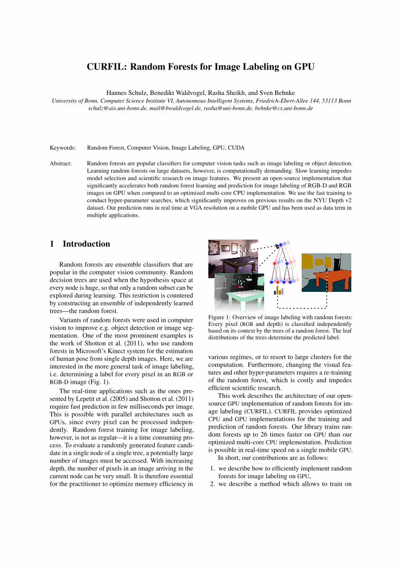
Variants of random forests were used in computervision to improve e.g. object detection or image seg-mentation. One of the most prominent examples isthe work of Shotton et al. (2011), who use randomforests in Microsoft’s Kinect system for the estimationof human pose from single depth images. Here, we areinterested in the more general task of image labeling,i.e. determining a label for every pixel in an RGB orRGB-D image (Fig. 1).

The real-time applications such as the ones pre-sented by Lepetit et al. (2005) and Shotton et al. (2011)require fast prediction in few milliseconds per image.This is possible with parallel architectures such asGPUs, since every pixel can be processed indepen-dently. Random forest training for image labeling,however, is not as regular—it is a time consuming pro-cess. To evaluate a randomly generated feature candi-date in a single node of a single tree, a potentially largenumber of images must be accessed. With increasingdepth, the number of pixels in an image arriving in thecurrent node can be very small. It is therefore essentialfor the practitioner to optimize memory efficiency in

Figure 1: Overview of image labeling with random forests:Every pixel (RGB and depth) is classified independentlybased on its context by the trees of a random forest. The leafdistributions of the trees determine the predicted label.

various regimes, or to resort to large clusters for thecomputation. Furthermore, changing the visual fea-tures and other hyper-parameters requires a re-trainingof the random forest, which is costly and impedesefficient scientific research.

This work describes the architecture of our open-source GPU implementation of random forests for im-age labeling (CURFIL). CURFIL provides optimizedCPU and GPU implementations for the training andprediction of random forests. Our library trains ran-dom forests up to 26 times faster on GPU than ouroptimized multi-core CPU implementation. Predictionis possible in real-time speed on a single mobile GPU.

In short, our contributions are as follows:

1. we describe how to efficiently implement randomforests for image labeling on GPU,

2. we describe a method which allows to train on

horizontally flipped images at significantly reducedcost,

3. we show that our GPU implementation is up to26 times faster for training (up to 48 times forprediction) than an optimized multi-core CPU im-plementation,

4. we show that simply by the now feasible optimiza-tion of hyper-parameters, we can improve perfor-mance in two image labeling tasks, and

5. we make our documented, unit-tested, and MIT-licensed source code publicly available1.

The remainder of this paper is organized as follows.After discussing related work, we introduce randomforests and our node tests in Sections 3 and 4, respec-tively. We describe our optimizations in Section 5.Section 6 analyzes speed and accuracy attained withour implementation.

2 Related Work

Random forests were popularized in computer vi-sion by Lepetit et al. (2005). Their task was to classifypatches at pre-selected keypoint locations, not—as inthis work—all pixels in an image. Random forestsproved to be very efficient predictors, while trainingefficiency was not discussed. Later work focused onimproving the technique and applying it to novel tasks.

Lepetit and Fua (2006) use random forests to clas-sify keypoints for object detection and pose estimation.They evaluate various node tests and show that whiletraining is increasingly costly, prediction can be veryfast.

The first GPU implementation for our task waspresented by Sharp (2008), who implements randomforest training and prediction for Microsoft’s Kinectsystem that achieves a prediction speed-up of 100 andtraining speed-up factor of eight on a GPU, comparedto a CPU. This implementation is not publicly avail-able and uses Direct3D which is only supported on theMicrosoft Windows platform.

An important real-world application of image la-beling with random forests is presented by Shottonet al. (2011). Human pose estimation is formulatedas a problem of determining pixel labels correspond-ing to body parts. The authors use a distributed CPUimplementation to reduce the training time, which isnevertheless one day for training three trees from onemillion synthetic images on a 1,000 CPU core cluster.Their implementation is also not publicly available.

Several fast implementations for general-purposerandom forests are available, notably in the scikit-

1https://github.com/deeplearningais/curfil/

learn machine learning library (Pedregosa et al., 2011)for CPU and CudaTree (Liao et al., 2013) for GPU.General random forests cannot make use of texturecaches optimized for images though, i.e., they treat allsamples separately. GPU implementations of general-purpose random forests also exist, but due to the irreg-ular access patterns when compared to image labelingproblems, their solutions were found to be inferior toCPU (Slat and Lapajne, 2010) or focused on prediction(Van Essen et al., 2012).

The prediction speed and accuracy of randomforests facilitates applications interfacing computer vi-sion with robotics, such as semantic prediction in com-bination with self localization and mapping (Stuckleret al., 2012) or 6D pose estimation (Rodrigues et al.,2012) for bin picking.

CURFIL was successfully used by Stuckler et al.(2013) to predict and accumulate semantic classesof indoor sequences in real-time, and by Muller andBehnke (2014) to significantly improve image labelingaccuracy on a benchmark dataset.

3 Random Forests

Random forests—also known as random decisiontrees or random decision forests—were independentlyintroduced by Ho (1995) and Amit and Geman (1997).Breiman (2001) coined the term “random forest”. Ran-dom decision forests are ensemble classifiers that con-sist of multiple decision trees—simple, commonlyused models in data mining and machine learning. Adecision tree consists of a hierarchy of questions thatare used to map a multi-dimensional input value to anoutput which can be either a real value (regression) ora class label (classification). Our implementation fo-cuses on classification but can be extended to supportregression.

To classify input x, we traverse each of the K de-cision trees Tk of the random forest F , starting at theroot node. Each inner node defines a test with a binaryoutcome (i.e. true or false). We traverse to the leftchild if the test is positive and continue with the rightchild otherwise. Classification is finished when a leafnode lk(x) is reached, where either a single class labelor a distribution p(c | lk(x)) over class labels c ∈ C isstored.

The K decision trees in a random forest are trainedindependently. The class distributions for the input xare collected from all leaves reached in the decisiontrees and combined to generate a single classification.Various combination functions are possible. We imple-ment majority voting and the average of all probability

q

w1

w2

h1

h2

o1

o2

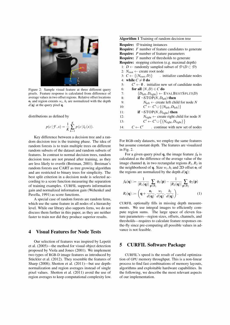
Figure 2: Sample visual feature at three different querypixels. Feature response is calculated from difference ofaverage values in two offset regions. Relative offset locationsoi and region extents wi, hi are normalized with the depthd(q) at the query pixel q.

distributions as defined by

p(c |F ,x) =1K

K

∑k=1

p(c | lk (x)).

Key difference between a decision tree and a ran-dom decision tree is the training phase. The idea ofrandom forests is to train multiple trees on differentrandom subsets of the dataset and random subsets offeatures. In contrast to normal decision trees, randomdecision trees are not pruned after training, as theyare less likely to overfit (Breiman, 2001). Breiman’srandom forests use CART as tree growing algorithmand are restricted to binary trees for simplicity. Thebest split criterion in a decision node is selected ac-cording to a score function measuring the separationof training examples. CURFIL supports informationgain and normalized information gain (Wehenkel andPavella, 1991) as score functions.

A special case of random forests are random ferns,which use the same feature in all nodes of a hierarchylevel. While our library also supports ferns, we do notdiscuss them further in this paper, as they are neitherfaster to train nor did they produce superior results.

4 Visual Features for Node Tests

Our selection of features was inspired by Lepetitet al. (2005)—the method for visual object detectionproposed by Viola and Jones (2001). We implementtwo types of RGB-D image features as introduced byStuckler et al. (2012). They resemble the features ofSharp (2008); Shotton et al. (2011)—but use depth-normalization and region averages instead of singlepixel values. Shotton et al. (2011) avoid the use ofregion averages to keep computational complexity low.

Algorithm 1 Training of random decision tree

Require: D training instancesRequire: F number of feature candidates to generateRequire: P number of feature parametersRequire: T number of thresholds to generateRequire: stopping criterion (e.g. maximal depth)

1: D← randomly sampled subset of D (D⊂D)2: Nroot ← create root node3: C← {(Nroot,D)} . initialize candidate nodes4: while C 6= /0 do5: C′← /0 . initialize new set of candidate nodes6: for all (N,D) ∈C do7:

(Dleft,Dright

)← EVALBESTSPLIT(D)

8: if ¬STOP(N,Dleft) then9: Nleft ← create left child for node N

10: C′←C′∪{(Nleft,Dleft)}11: if ¬STOP(N,Dright) then12: Nright ← create right child for node N13: C′←C′∪

{(Nright,Dright

)}14: C←C′ . continue with new set of nodes

For RGB-only datasets, we employ the same featuresbut assume constant depth. The features are visualizedin Fig. 2.

For a given query pixel q, the image feature fθ iscalculated as the difference of the average value of theimage channel φi in two rectangular regions R1,R2 inthe neighborhood of q. Size wi,hi and 2D offset oi ofthe regions are normalized by the depth d(q):

fθ(q) :=1

|R1(q)| ∑p∈R1

φ1(p)−1

|R2(q)| ∑p∈R2

φ2(p)

Ri(q) :=(

q+oi

d(q),

wi

d(q),

hi

d(q)

). (1)

CURFIL optionally fills in missing depth measure-ments. We use integral images to efficiently com-pute region sums. The large space of eleven fea-ture parameters—region sizes, offsets, channels, andthresholds—requires to calculate feature responses on-the-fly since pre-computing all possible values in ad-vance is not feasible.

5 CURFIL Software Package

CURFIL’s speed is the result of careful optimiza-tion of GPU memory throughput. This is a non-linearprocess to find fast combinations of memory layouts,algorithms and exploitable hardware capabilities. Inthe following, we describe the most relevant aspectsof our implementation.

Block (0, D) Block (1, D) Block (2, D)

Block (0, 1) Block (1, 1) Block (2, 1)

Block (X, D)

Block (X, 1)

Block (0, 0) Block (1, 0) Block (2, 0) Block (X, 0)

…scheduling order

Feature

Sam

ple

(a) Feature Response Kernel

Block (0, F) Block (1, F) Block (2, F)

Block (0, 1) Block (1, 1) Block (2, 1)

Block (T, F)

Block (T, 1)

Block (0, 0) Block (1, 0) Block (2, 0) Block (T, 0)

…scheduling order

Threshold

Fea

ture

Thread Block (2,0)

Thread 0 Thread 1 Thread 2 Thread 3 Thread X

…

(b) Histogram Aggegation Kernel

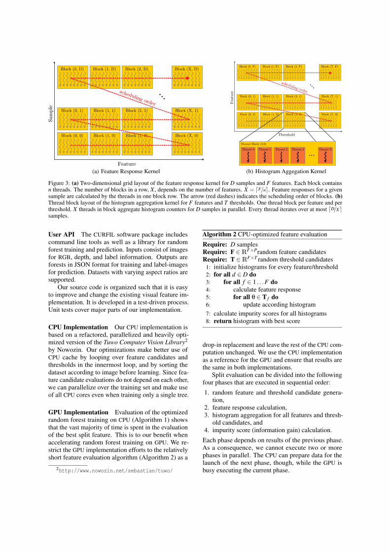
Figure 3: (a) Two-dimensional grid layout of the feature response kernel for D samples and F features. Each block containsn threads. The number of blocks in a row, X , depends on the number of features. X = dF/ne. Feature responses for a givensample are calculated by the threads in one block row. The arrow (red dashes) indicates the scheduling order of blocks. (b)Thread block layout of the histogram aggregation kernel for F features and T thresholds. One thread block per feature and perthreshold. X threads in block aggregate histogram counters for D samples in parallel. Every thread iterates over at most dD/Xesamples.

User API The CURFIL software package includescommand line tools as well as a library for randomforest training and prediction. Inputs consist of imagesfor RGB, depth, and label information. Outputs areforests in JSON format for training and label-imagesfor prediction. Datasets with varying aspect ratios aresupported.

Our source code is organized such that it is easyto improve and change the existing visual feature im-plementation. It is developed in a test-driven process.Unit tests cover major parts of our implementation.

CPU Implementation Our CPU implementation isbased on a refactored, parallelized and heavily opti-mized version of the Tuwo Computer Vision Library2

by Nowozin. Our optimizations make better use ofCPU cache by looping over feature candidates andthresholds in the innermost loop, and by sorting thedataset according to image before learning. Since fea-ture candidate evaluations do not depend on each other,we can parallelize over the training set and make useof all CPU cores even when training only a single tree.

GPU Implementation Evaluation of the optimizedrandom forest training on CPU (Algorithm 1) showsthat the vast majority of time is spent in the evaluationof the best split feature. This is to our benefit whenaccelerating random forest training on GPU. We re-strict the GPU implementation efforts to the relativelyshort feature evaluation algorithm (Algorithm 2) as a

2http://www.nowozin.net/sebastian/tuwo/

Algorithm 2 CPU-optimized feature evaluation

Require: D samplesRequire: F ∈RF×Prandom feature candidatesRequire: T ∈RF×T random threshold candidates

1: initialize histograms for every feature/threshold2: for all d ∈ D do3: for all f ∈ 1 . . .F do4: calculate feature response5: for all θ ∈ T f do6: update according histogram7: calculate impurity scores for all histograms8: return histogram with best score

drop-in replacement and leave the rest of the CPU com-putation unchanged. We use the CPU implementationas a reference for the GPU and ensure that results arethe same in both implementations.

Split evaluation can be divided into the followingfour phases that are executed in sequential order:

1. random feature and threshold candidate genera-tion,

2. feature response calculation,3. histogram aggregation for all features and thresh-

old candidates, and4. impurity score (information gain) calculation.

Each phase depends on results of the previous phase.As a consequence, we cannot execute two or morephases in parallel. The CPU can prepare data for thelaunch of the next phase, though, while the GPU isbusy executing the current phase.

class 0

…0 1 2 3 C

sharedmemory

…

globalmemory

left counter

right counter

class

thread 0 1 2 3 4 5 6 7 2C

…

…

class 1 class C

…

Figure 4: Reduction of histogram counters. Every thread sums to a dedicated left and right counter (indicated by differentcolors) for each class (first row). Counters are reduced in a subsequent phase. The last reduction step stores counters in sharedmemory, such that no bank conflicts occur when copying to global memory.

5.1 GPU Kernels

Random Feature and Threshold Candidate Gener-ation A significant amount of training time is usedfor generating random feature candidates. The totaltime for feature generation increases per tree levelsince the number of nodes increases as trees are grown.

The first step in the feature candidate generationis to randomly select feature parameter values. Theseare stored in a F×11 matrix for F feature candidatesand eleven feature parameters of Eq. (1). The sec-ond step is the selection of one or more thresholdsfor every feature candidate. Random threshold can-didates can either be obtained by randomly samplingfrom a distribution or by sampling feature responses oftraining instances. We implement the latter approach,which allows for greater flexibility if features or im-age channels are changed. For every feature candidategeneration, one thread on the GPU is used and all Tthresholds for a given feature are sampled by the samethread.

In addition to sorting samples according to the im-age they belong to, feature candidates are sorted by thefeature type, channels used, and region offsets. Sort-ing reduces branch divergence and improves spatiallocality, thereby increasing the cache hit rate.

Feature Response Calculation The GPU imple-mentation uses a similar optimization technique tothe one used on the CPU, where loops in the featuregeneration step are rearranged in order to improvecaching.

We used one thread to calculate the feature re-sponse for a given feature and a given training sample.Figure 3(a) shows the thread block layout for the fea-ture response calculation. A row of blocks calculatesall feature responses for a given sample. A column ofblocks calculates the feature responses for a given fea-

ture over all samples. The dotted red arrow indicatesthe order of thread block scheduling. The executionorder of thread blocks is determined by calculatingthe Block ID bid. In the two-dimensional case, it isdefined as

bid = blockIdx.x+gridDim.x︸ ︷︷ ︸blocks in row

·blockIdx.y︸ ︷︷ ︸sample ID

.

The number of features can exceed the maximum num-ber of threads in a block, hence, the feature responsecalculation is split into several thread blocks. We usethe x coordinate in the grid for the feature block toensure that all features are evaluated before the GPUcontinues with the next sample. The y coordinate in thegrid assigns training samples to thread blocks. Threadsreconstruct their feature ID f using block size, threadand block ID by calculating

f = threadIdx.x+ blockDim.x︸ ︷︷ ︸threads in block row

· blockIdx.x︸ ︷︷ ︸block index in grid row

.

After sample data and feature parameters areloaded, the kernel calculates a single feature responsefor a depth or color feature by querying four pixels inan integral image and carrying out simple arithmeticoperations to calculate the two regions sums and theirdifference.

Histogram Aggregation Feature responses are ag-gregated into class histograms. Counters for his-tograms are maintained in a four-dimensional matrixof size F×T×C×2 for F features, T thresholds, Cclasses, and the two left and right children of a split.

To compute histograms, the iteration over featuresand thresholds is implemented as thread blocks in atwo-dimensional grid on GPU; one thread block perfeature and threshold. This is depicted in Fig. 3(b).Each thread block slices samples into partitions such

that all threads in the block can aggregate histogramcounters in parallel.

Histogram counters for one feature and thresholdare kept in the shared memory, and every thread getsa distinct region in the memory. For X threads andC classes, 2XC counters are allocated. An additionalreduction phase is then required to reduce the countersto a final sum matrix of size C×2 for every feature andthreshold.

Figure 4 shows histogram aggregation and sum re-duction. Every thread increments a dedicated counterfor each class in the first phase. In the next phase, weiterate over all C classes and reduce the counters ofevery thread in O(logX) steps, where X is the numberof threads in a block. In a single step, every threadcalculates the sum of two counters. The loop over allclasses can be executed in parallel by 2C threads thatcopy the left and right counters of C classes.

The binary reduction of counters (Fig. 4) has aconstant runtime overhead per class. The reduction ofcounters for classes without samples can be skipped,as all counters are zero in this case.

Impurity Score Calculation Computing impurityscores from the four-dimensional counter matrix is thelast of the four training phases that are executed onGPU.

In the score kernel computation, 128 threads perblock are used. A single thread computes the scorefor a different pair of features and thresholds. It loads2C counters from the four-dimensional counter matrixin global memory, calculates the impurity score andwrites back the resulting score to global memory.

The calculated scores are stored in a T×F matrixfor T thresholds and F features. The matrix is thenfinally transferred from device to host memory space.

Undefined Values Image borders and missing depthvalues (e.g. due to material properties or camera dis-parity) are represented as NaN, which automaticallypropagates and causes comparisons to produce false.This is advantageous, since no further checks are re-quired and the random forest automatically learns todeal with missing values.

5.2 Global Memory Limitations

Slicing of Samples Training arbitrarily largedatasets with many samples can exceed the storagecapacity of global memory. The feature response ma-trix of size D×F scales linearly in the number of sam-ples D and the number of feature candidates F . Wecannot keep the entire matrix in global memory ifD or F is too large. For example, training a dataset

with 500 images, 2000 samples per image, 2000 fea-ture candidates and double precision feature responses(64 bit) would require 500 ·2000 ·2000 ·64bit≈ 15GBof global memory for the feature response matrix inthe root node split evaluation.

To overcome this limitation, we split samples intopartitions, sequentially compute feature responses, andaggregate histograms for every partition. The maxi-mum possible partition size depends on the availableglobal memory of the GPU.

Image Cache Given a large dataset, we might not beable to keep all images in the GPU global memory. Weimplement an image cache with a last recently used(LRU) strategy that keeps a fixed number of images inmemory. Slicing samples ensures that a partition doesnot require more images than can be fit into the cache.

Memory Pooling To avoid frequent memory alloca-tions, we reuse memory that is already allocated butno longer in use. Due to the structure of random deci-sion trees, evaluation of the root node split criterion isguaranteed to require the largest amount of memory,since child nodes always contain less or equal samplesthan the root node. Therefore, all data structures haveat most the size of the structures used for calculatingthe root node split. With this knowledge, we are ableto train a tree with no memory reallocation.

5.3 Extensions

Hyper-Parameter Optimization Cross-validatingall the hyper-parameters is a requirement for modelcomparison, and random forests have quite a fewhyper-parameters, such as stopping criteria for split-ting, number of features and thresholds generated, andthe feature distribution parameters.

To facilitate model comparison, CURFIL includessupport for cross-validation and a client for an in-formed search of the best parameter setting using Hy-peropt (Bergstra et al., 2011). This allows to leveragethe improved training speed to run many experimentsserially and in parallel.

Image Flipping To avoid overfitting, the dataset canbe augmented using transformations of the trainingdataset. One possibility is to add horizontally flippedimages, since most tasks are invariant to this transfor-mation. CURFIL supports training horizontally flippedimages with reduced overhead.

Instead of augmenting the dataset with flipped im-ages and doubling the number of pixels used for train-ing, we horizontally flip each of the two rectangularregions used as features for a sampled pixel. This is

Table 1: Comparison of random forest training time (in min-utes) on a quadcore CPU and two non-mobile GPUs. Randomforest parameters were chosen for best accuracy.

NYU MSRC

Device time factor time factor

i7–4770K 369 1.0 93.2 1.0Tesla K20c 55 6.7 5.1 18.4GTX Titan 24 15.4 3.4 25.9

Table 2: Random forest prediction time in milliseconds, onRGB-D images at original resolution, comparing speed ona recent quadcore CPU and various GPUs. Random forestparameters are are chosen for best accuracy.

NYU MSRC

Device time factor time factor

i7-440K 477 1 409 1GTX 675M 28 17 37 11Tesla K20c 14 34 10 41GTX Titan 12 39 9 48

equivalent to computing the feature response of thesame feature for the same pixel on an actual flippedimage. Histogram counters are then incremented fol-lowing the binary test of both feature responses. Theimplicit assumption here is that the samples generatedthrough flipping are independent.

The paired sample is propagated down a tree untilthe outcome of a node binary test is different for thetwo feature responses, indicating that a sample andits flipped counterpart should split into different direc-tions. A copy of the sample is then created and addedto the samples list of the other node child.

This technique reduces training time since choos-ing independent samples from actually flipped imagesrequires loading more images in memory during thebest split evaluation step. Since our performance islargely bounded by memory throughput, dependentsampling allows for higher throughput at no cost inaccuracy.

6 Experimental Results

We evaluate our library on two common image labelingtasks, the NYU Depth v2 dataset and the MSRC-21dataset. We focus on the processing speed, but alsodiscuss the prediction accuracies attained. Note thatthe speed between datasets is not comparable, sincedataset sizes differ and the forest parameters werechosen separately for best accuracy.

The NYU Depth v2 dataset by Silberman et al.(2012) contains 1,449 densely labeled pairs of aligned

Table 3: Segmentation accuracies on NYU Depth v2 datasetof our random forest compared to state-of-the-art methods.We used the same forest as in the training/prediction timecomparisons of Tables 1 and 2.

Accuracy [%]

Method Pixel Class

Silberman et al. (2012) 59.6 58.6Couprie et al. (2013) 63.5 64.5Our random forest∗ 68.1 65.1Stuckler et al. (2013)∗∗ 70.6 66.8Hermans et al. (2014) 68.1 69.0Muller and Behnke (2014)∗∗ 72.3 71.9∗ see main text for hyper-parameters used∗∗ based on our random forest prediction

RGB-D images from 464 indoor scenes. We focus onthe semantic classes ground, furniture, structure, andprops defined by Silberman et al..

To evaluate our performance without depth, we usethe MSRC-21 dataset3. Here, we follow the literaturein treating rarely occuring classes horse and mountainas void and train/predict the remaining 21 classes onthe standard split of 335 training and 256 test images.

Tables 1 and 2 show random forest training andprediction times, respectively, on an Intel Core i7-4770K (3.9 GHz) quadcore CPU and various NVidiaGPUs. Note that the CPU version is using all cores.

For the RGB-D dataset, training speed is improvedfrom 369 min to 24 min, which amounts to a speed-upfactor of 15. Dense prediction improves by factor of39 from 477 ms to 12 ms.

Training on the RGB dataset is finished after3.4 min on a GTX Titan, which is 26 times faster thanCPU (93 min). For prediction, we achieve a speed-upof 48 on the same device (9 ms vs. 409 ms).

Prediction is fast enough to run in real time evenon a mobile GPU (GTX 675M, on a laptop computerfitted with a quadcore i7-3610QM CPU), with 28 ms(RGB-D) and 37 ms (RGB).

Our implementation is fast enough to train hun-dreds of random decision trees per day on a sin-gle GPU. This fast training enabled us to conductan extensive parameter search with cross-validationto optimize segmentation accuracy of a random for-est trained on the NYU Depth v2 dataset (Silbermanet al., 2012). Table 3 shows that we outperform otherstate-of-the art methods simply by using a randomforest with optimized parameters. Our implementa-tion was used in two publications which improved theresults further by 3D accumulation of predictions inreal time (Stuckler et al., 2013) and superpixel CRFs

3http://jamie.shotton.org/work/data.html

Figure 5: Image labeling examples on NYU Depth v2 dataset. Left to right: RGB image, depth visualization, ground truth,random forest segmentation.

(Muller and Behnke, 2014). This shows that efficienthyper-parameter search is crucial for model selection.Example segmentations are displayed in Figs. 5 and 6.

Methods on the established RGB-only MSRC-21benchmark are so advanced that their accuracy cannotsimply be improved by a random forest with betterhyper parameters. Our pixel and class accuracies forMSRC-21 are 59.2% and 47.0%, respectively. Thisis still higher than other published work using RFas the baseline method, such as 49.7 % and 34.5 %by Shotton et al. (2008). However, as Shotton et al.and the above works show, random forest predictionsare fast and constitute a good initialization for othermethods such as conditional random fields.

Finally, we trained the MSRC-21 dataset by aug-menting the dataset with horizontally flipped imagesusing the naıve approch and our proposed method.The naıve approach doubles both the total number ofsamples and the number of images, which quadruplesthe training time to 14.4 min. Accuracy increases to60.6 % and 48.6 % for pixel and class accuracy, re-spectively. With paired samples (introduced in Sec-tion 5.3), we reduce the runtime by a factor of two(to now 7.48 min) at no cost in accuracy (60.9 % and49.0 %). The remaining difference in speed is mainlyexplained by the increased number of samples, thusthe training on flipped images has very little overhead.

Random Forest Parameters The hyper-parameterconfigurations for which we report our timing andaccuracy results were found with cross-validation. Thecross-validation outcome varies between datasets.

For the NYU Depth v2 dataset, we used three

trees with 4537 samples / image, 5729 feature candi-dates / node, 20 threshold candidates, a box radius of111 px, a region size of 3, tree depth 18 levels, andminimum samples in leaf nodes 204.

For MSRC-21, we found 10 trees, 4527 sam-ples / image, 500 feature candidates / node, 20 thresh-old candidates, a box radius of 95 px, a region size of12, tree depth 25 levels, and minimum samples in leafnodes 38 to yield best results.

7 Conclusion

We provide an accelerated random forest imple-mentation for image labeling research and applications.Our implementation achieves dense pixel-wise classifi-cation of VGA images in real-time on a GPU. Trainingis accelerated on GPU by a factor of up to 26 comparedto an optimized CPU version. The experimental resultsshow that our fast implementation enables effectiveparameter searches that find solutions which outper-form state-of-the art methods. CURFIL prepares theground for scientific progress with random forests, e.g.through research on improved visual features.

REFERENCES

Amit, Y. and Geman, D. (1997). Shape quantization andrecognition with randomized trees. Neural computation,9(7):1545–1588.

Bergstra, J., Bardenet, R., Bengio, Y., Kegl, B., et al. (2011).Algorithms for hyper-parameter optimization. In NeuralInformation Processing Systems (NIPS).

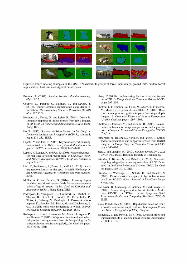
Figure 6: Image labeling examples on the MSRC-21 dataset. In groups of three: input image, ground truth, random forestsegmentation. Last row shows typical failure cases

Breiman, L. (2001). Random forests. Machine learning,45(1):5–32.

Couprie, C., Farabet, C., Najman, L., and LeCun, Y.(2013). Indoor semantic segmentation using depth in-formation. The Computing Resource Repository (CoRR)abs/1301.3572.

Hermans, A., Floros, G., and Leibe, B. (2014). Dense 3dsemantic mapping of indoor scenes from rgb-d images.In Int. Conf. on Robotics and Automation (ICRA), HongKong. IEEE.

Ho, T. (1995). Random decision forests. In Int. Conf. onDocument Analysis and Recognition (ICDAR), volume 1,pages 278–282. IEEE.

Lepetit, V. and Fua, P. (2006). Keypoint recognition usingrandomized trees. Pattern Analysis and Machine Intelli-gence, IEEE Transactions on, 28(9):1465–1479.

Lepetit, V., Lagger, P., and Fua, P. (2005). Randomized treesfor real-time keypoint recognition. In Computer Visionand Pattern Recognition (CVPR), Conf. on, volume 2,pages 775–781.

Liao, Y., Rubinsteyn, A., Power, R., and Li, J. (2013). Learn-ing random forests on the gpu. In NIPS Workshop onBig Learning: Advances in Algorithms and Data Manage-ment.

Muller, A. C. and Behnke, S. (2014). Learning depth-sensitive conditional random fields for semantic segmen-tation of rgb-d images. In Int. Conf. on Robotics andAutomation (ICRA), Hong Kong. IEEE.

Pedregosa, F., Varoquaux, G., Gramfort, A., Michel, V.,Thirion, B., Grisel, O., Blondel, M., Prettenhofer, P.,Weiss, R., Dubourg, V., Vanderplas, J., Passos, A., Cour-napeau, D., Brucher, M., Perrot, M., and Duchesnay, E.(2011). Scikit-learn: Machine learning in Python. Journalof Machine Learning Research, 12:2825–2830.

Rodrigues, J., Kim, J., Furukawa, M., Xavier, J., Aguiar, P.,and Kanade, T. (2012). 6D pose estimation of texturelessshiny objects using random ferns for bin-picking. In In-telligent Robots and Systems (IROS), Int. Conf. on, pages3334–3341. IEEE.

Sharp, T. (2008). Implementing decision trees and forestson a GPU. In Europ. Conf. on Computer Vision (ECCV),pages 595–608.

Shotton, J., Fitzgibbon, A., Cook, M., Sharp, T., Finocchio,M., Moore, R., Kipman, A., and Blake, A. (2011). Real-time human pose recognition in parts from single depthimages. In Computer Vision and Pattern Recognition(CVPR), Conf. on, pages 1297–1304.

Shotton, J., Johnson, M., and Cipolla, R. (2008). Seman-tic texton forests for image categorization and segmenta-tion. In Computer Vision and Pattern Recognition (CVPR),Conf. on.

Silberman, N., Hoiem, D., Kohli, P., and Fergus, R. (2012).Indoor segmentation and support inference from RGBDimages. In Europ. Conf. on Computer Vision (ECCV),pages 746–760.

Slat, D. and Lapajne, M. (2010). Random Forests for CUDAGPUs. PhD thesis, Blekinge Institute of Technology.

Stuckler, J., Biresev, N., and Behnke, S. (2012). Semanticmapping using object-class segmentation of RGB-D im-ages. In Intelligent Robots and Systems (IROS), Int. Conf.on, pages 3005–3010. IEEE.

Stuckler, J., Waldvogel, B., Schulz, H., and Behnke, S.(2013). Dense real-time mapping of object-class seman-tics from RGB-D video. Journal of Real-Time ImageProcessing.

Van Essen, B., Macaraeg, C., Gokhale, M., and Prenger, R.(2012). Accelerating a random forest classifier: Multi-core, GP-GPU, or FPGA? In Int. Symp. on Field-Programmable Custom Computing Machines (FCCM).IEEE.

Viola, P. and Jones, M. (2001). Rapid object detection usinga boosted cascade of simple features. In Computer Visionand Pattern Recognition (CVPR), Conf. on.

Wehenkel, L. and Pavella, M. (1991). Decision trees andtransient stability of electric power systems. Automatica,27(1):115–134.