Cumulative score charts

CUMULATIVE SCORE CHARTS GEORGE BOX

Center for Quality & Productivity Improvement, University of Wisconsin-Madison, Madison, WI 53705, U.S. A.

AND

JOSB R A M ~ R E Z Quality Reliability Semiconductor Operations, Digital Equipment Corporation, 77 Reed Road, Hudson, MA 01 749-9987, U. S. A

SUMMARY

Shewhart charts are direct plots of the data and they have the potential to detect departures from statistical stability of unanticipated kinds. However, when one can identify in advance a kind of departure specifically feared, then a more sensitive detection statistic can be developed for that specific possibility.

In this paper Cuscore statistics are developed for this purpose which can be used as an adjunct to the Shewhart chart. These statistics use an idea due to Box and Jenkins' which is in turn an application of Fisher's score statistic. This article shows how the resulting procedures relate to Wald-Barnard sequential tests and to Cusum statistics which are special cases of Cuscore statistics. The ideas are

' illustrated by a number of examples. These concern the detection in a noisy environment of (a) an intermittent sine wave, (b) a change in slope of a line, (c) a change in an exponential smoothing constant and (d) a change from a stationary to a non-stationary state in a process record.

KEY WORDS Control charts Cusums Sequential test

INTRODUCTION

Process control can have different objectives and consequently can take different forms. One impor- tant objective is process regulation achieved, for example, by automatic feedback and feedforward control schemes designed to maintain a quality characteristic close to target. Statistical considerations associated with such schemes have been discussed, for example, by Box and Jenkins,* A ~ t r o m , " ~ MacGregor,s and Box and Kramer."

This paper concerns the situation where the object is not primarily to regulate but to monitor the process. Such monitoring provides sequential verification of the continuous stability of the process once a state of statistical control has been achieved, and allows detection of deviations from the state leading to an appropriate search for assignable causes. Such process monitoring may be achieved, for example, by using a Shewhart chart.

One of the many virtues of the Shewhart chart is that it is a direct plot of the actual data and so can expose types of deviations from statistical stability, of a totally unexpected kind. Thus it can serve in an inductive role. Inspection of such a chart might, for example, show that every fifth observation was low as compared to the mean of the previous four which might in turn lead to the discovery of an assignable cause previously not even thought of. However, this property of potential response to global alternatives also ensures that the Shewhart chart will not be as sensitive to some specific deviation from randomness as a correspondingly specially chosen procedure.

Non-stationarity

When such a specific kind of deviation is feared, therefore, it is appropriate to employ a procedure especially sensitive to that possibility and to use it in addition to the overall Shewhart chart. The problem has been likened by Box' to that faced by a small country wishing to install an early warning radar system against air attack. In addition to a multi-directional screen it would be wise to add very sensitive radar beams in certain directions known to be likely sources of aggression.

In the monitoring of quality, one such additional specific procedure employs the Page-Barnard cumul- ative sum (Cusum) chart.X,Y Such a chart is partic- ularly sensitive to small changes in the mean level of a process characteristic, indicated by a change of slope of the Cusum. The sensitivity of this procedure arises from its equivalence to a Wald-Barnard sequential likelihood test for change in mean. Equiv- alently, it can be regarded as a test based on the accumulated Fisher score statistic. Such charts can provide the basis for formal tests of statistical sig- nificance, but have often been used informally to track down assignable causes evidenced by small changes in mean level. For example, at a large chemical plant for the manufacture of ammonia in which accurate metering of gas flow was critical, a Cusum chart for gas flow showed marked changes of slope indicating small shifts in mean on specific days which were about four weeks apart. Careful investigation revealed that these changes occurred close to times at which the gas flowmeters had been recalibrated. New calibration procedures eliminated the problem. Used in this diagnostic way Cusum

O748-8017/92/O1OO17-11$O5.50 0 1992 by John Wiley & Sons, Ltd.

Received 1 July 1991 Revised 1 1 September 1991

18 G . BOX AND J . RAMfREZ

charts are a valuable adjunct to, for example, Ishika- wa's 'seven tools' and similar exploratory methods for tracking down the causes of problems and so improving quality.

Now, occasions occur when some specific kind of deviation other than a change in mean is feared as a likely possibility. To cope with this kind of problem, in an unpublished report, Box and Jenkins' proposed a general cumulative score statistic. Although the immediate objective of these authors was to warn of possible changes in the parameters of time series models, the concept has much broader applicability.

THE CUSCORE STATISTIC

Consider a statistical model written in the form

a, = a,(y,,x,,8), t = 1,2, ..., n (1)

where y, are observations, 8 is some unknown parameter and the x,s are known independent variables. Then standard normal theory models assume that when 8 is the true value of the unknown parameter, the resulting a,s are a sequence of independently identically normally distributed random variables with mean zero and variance a3 = d, which we will call a white noise sequence. Thought of in this way, statistical models are recipes for reducing data to 'white noise'.

Apart from a constant, the log likelihood for 8 = O0 is then

where the a,,,s are obtained by setting 8 = O0 in (1) and unless otherwise stated, 2 will indicate summation from t = 1,2, ..., n. If we now write

then

(3)

and we shall refer to

as the Cuscore associated with the parameter value

Now expanding a, about a,,, the following formula is exact if the model is linear in 8 and approximate otherwise:

e = eo.

Whence we see that if the value of the parameter is not equal to O0 an increment of the discrepancy vector d,,, is added to the vector a,. The Cuscore statistic equation (4) which sequentially correlates a,,, with df0 is thus continuously searching for the presence of that particular discrepancy vector. Equivalently since (6-Oo) = Za,,&Z,d2,) is the least squares estimator of 8-B0

Q = (6 - % ) W o (6 )

When plotted against n the Cuscore can thus be expected to provide a very sensitive check for changes in 8, and such changes will be indicated by a change in slope of the plot just as changes in the mean are indicated by a change in slope of the Cusum plot. By noticing at which specific times changes in slope have occurred, the Cuscore may thus be used to provide clues as to the time of occurrence, and hence possibly of the identity of specific problems. In addition, as we discuss later, approximate formal significance tests can be made if these are desired.

Detecting a sine wave buried in noise

As a first illustration, consider an industrial process in which trouble has been experienced with a characteristic harmonic cycling about a target value T at a particular period and phase, and suppose that although action has been taken which seems to have solved the problem it is feared that it might recur. A test procedure is needed which will give the earliest possible warning of its recurrence.

Suppose the sine wave has amplitude 8 and period p, then the model is

y , = T + esin(2dp) + a,

or

a, = y , - T - Osin(2dp) (7)

When the process is operating correctly, 8 = O0 = 0, and there will be no sine component in y, - T. Since d,,, = sin(2dp) the Cuscore statistic which is looking for a recurrence of the sine component is

Qo = 2 ( y t - T)sin(2nt/p)

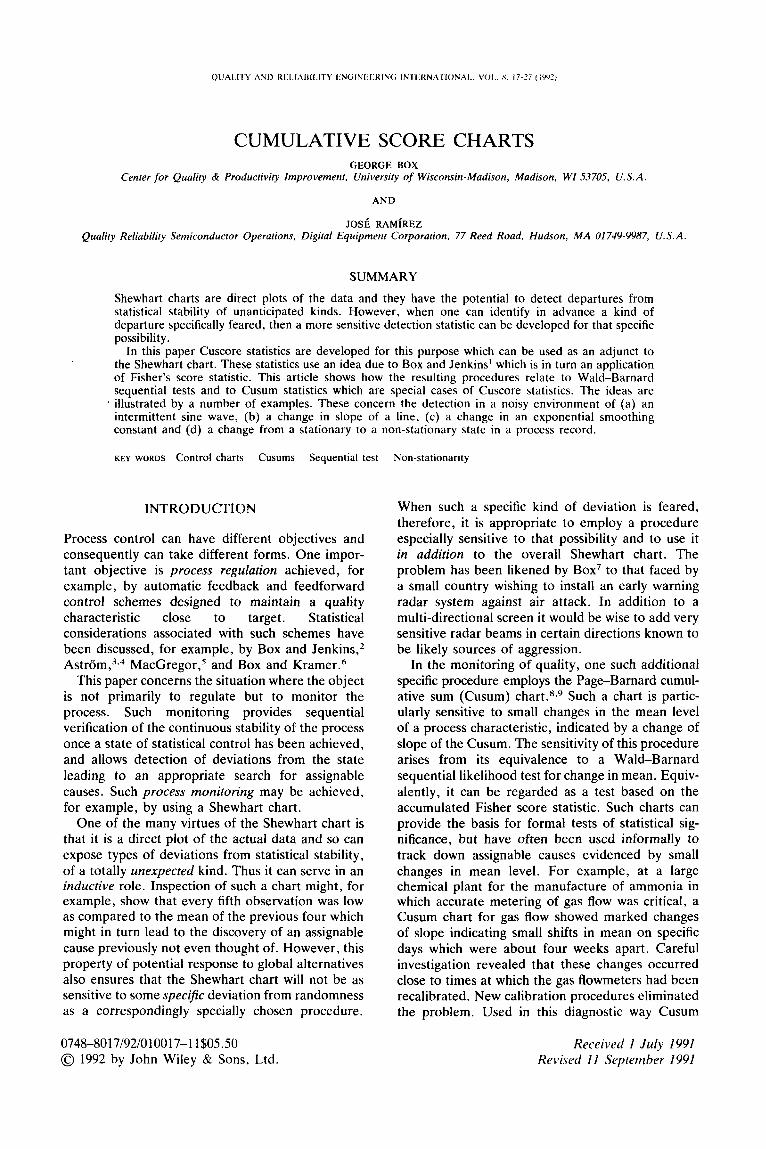
For illustration, 144 random normal deviates were generated with standard deviation u = 1 and a sine wave with period 12 and amplitude 8 = 4 was added at the 48th observation and then omitted after the 96th observation, as shown in Figure l(a), which also shows a Shewhart chart for the composite series obtained by adding the sine wave to the white noise. It will be seen that sine wave is effectively hidden

CUMULATIVE SCORE CHARTS

3.5-

3.0

19

3 0

20

-20

-30

---t--f--+.+-- +--+-.-+--+--+-- 0 10 20 30 40 50 60 70 80 90 100 I10 120 130 140

t Figure 1 . (a). A series consisting of an intermittent sine wave (continuous line) buried in noise generated from random normal deviates

having standard deviation unity. The fluctuating series is the sum of the two components

24-

22--

20- -

1e--

10--

14-- C U s 12--

C

0 lo-- r

8--

8- -

4- -

t

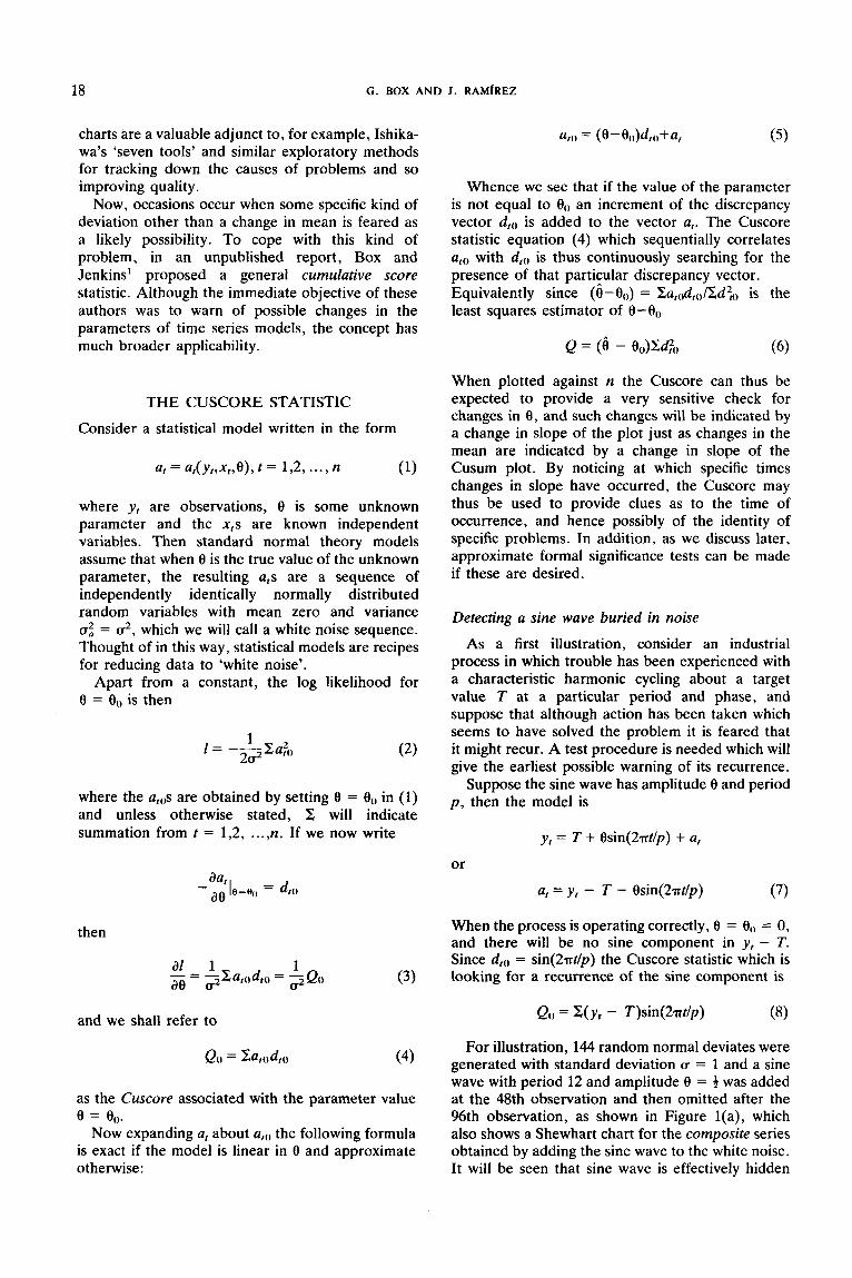
Figure 1. (b). A Cuscore chart for series of Figure l(a).

20 G . BOX A N D J . RAMiREZ

141 13

12--

11--

C

e lo--

n

e

e 8--

7--

C

u w-

e

-0 10 20 3b 40 SO 60 70 60 90

Jl \ , /

e = o

I I i

100 110 120 130 140 150

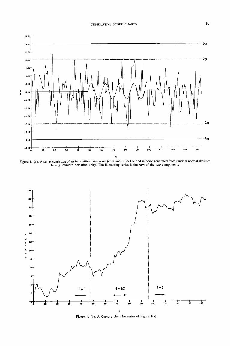
t Figure 1 . (c). A centred Cuscore chart appropriate to compare 0(,. with 0 , = 0.5 for a = 0,01 signalling a change after observation 86

in the noise. The appearance and disappearance of the sine wave is, however, quite evident in the Cuscore chart of Figure l (b) in which

Q = C ( y , - T)s in (d6) (9)

is plotted against c . Figure l(c) is discussed later.

THE LINEAR MODEL

More generally consider this approach for the linear model

y , = Ox, + a, (10)

In this case

and the Cuscore statistic is

In the particular special case where x, = 1 = d,,, for t = 1,2 ,..., n, the test is for a change in mean and the Cuscore is the familiar Cusum statistic Q,, = Cot, - Oo) with Oo as the reference value. The sine wave example was also a special case of this linear model in which x, = s i n ( d 6 ) = d,,,.

Detecting a change in gradient

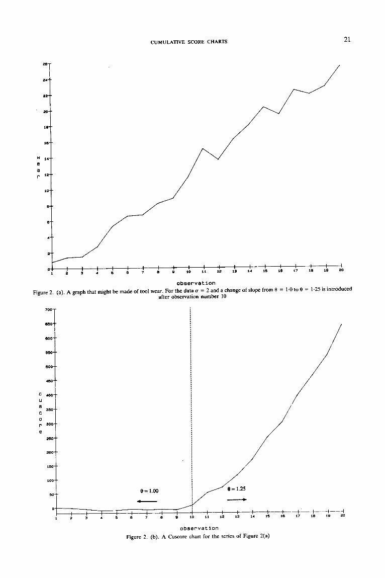
As a further application suppose y , is the amount of wear of a tool observed at time t. Suppose also that for a properly operating tool the rate of wear per unit interval is Oo. Suppose that, should the wear be greater than 00, we wish to find this out as quickly as possible. Denoting the wear by y, the model is

y , = Or + a,

or

a, = y , - Or (13)

and the Cuscore statistic is

Notice that for this problem it might have seemed appropriate to simply plot the Cusum of the residuals Z(y, - Oat). However, the likelihood argument tells us that a more sensitive statistic will result if the successive residuals are multiplied by 1, 2,3, and so on.

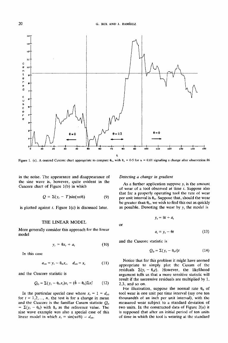
For illustration, suppose the normal rate O0 of tool wear is one unit per time interval (say one ten thousandth of an inch per unit interval), with the measured wear subject to a standard deviation of two units. In the constructed data of Figure 2(a) it is supposed that after an initial period of ten units of time in which the tool is wearing at the standard

CUMULATIVE SCORE CHARTS

700-

650--

600--

sso-

soo--

450--

400-- U S

C

0 r 300--

350--

e 2so--

200--

150--

loo--

50--

0

21

-

/ / I . I

e = 1.00 8 = 1.25

1 ! --I---- I I ---f----t--t-+---+.- -+--.+-+ -.--I I 2 3 4 5 6 7 B B 10 I1 12 13 14 IS 16 17 10 19 20

observation Figure 2. (a). A graph that might be made of tool wear. For the data u = 2 and a change of slope from 0 = 1.0 to 8 = 1.25 is introduced

after observation number 10

observation Figure 2. (b). A Cuscore chart for the series of Figure 2(a)

22 G . BOX AND J . RAMfREZ

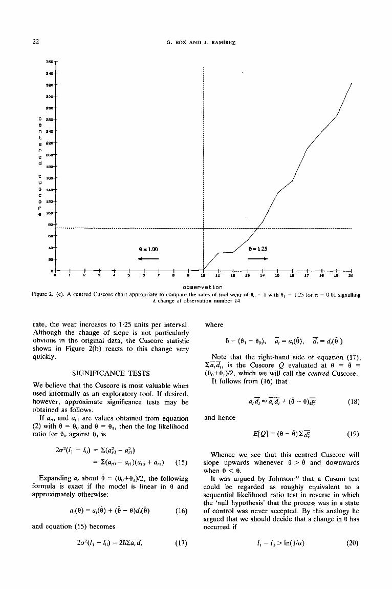
observation Figure 2. (c). A centred Cuscore chart appropriate to compare the rates of tool wear of 0,, = 1 with 0 , = 1.25 for (Y = 0.01 signalling

a change at observation number 14

rate, the wear increases to 1-25 units per interval. Although the change of slope is not particularly obvious in the original data, the Cuscore statistic shown in Figure 2(b) reacts to this change very quickly.

SIGNIFICANCE TESTS

We believe that the Cuscore is most valuable when used informally as an exploratory tool. If desired, however, approximate significance tests may be obtained as follows.

If a,,, and a,] are values obtained from equation (2) with 8 = 8,) and 8 = 8, , then the log likelihood ratio for 0,) against is

Expanding a, about 6 = (8,)+01)/2, the following formula is exact if the model is linear in 8 and approximately otherwise:

and equation (15) becomes

where

Note that the right-hand side of equation (17), xzd,, is the Cuscore Q evaluated at 0 = 6 = (80+81)/2, which we will call the centred Cuscore.

It follows from (16) that

and hence

E[Q] = (0 - 6 ) Z s

Whence we see that this centred Cuscore will slope upwards whenever 0 > 6 and downwards when 8 < 6.

It was argued by Johnson'" that a Cusum test could be regarded as roughly equivalent to a sequential likelihood ratio test in reverse in which the 'null hypothesis' that the process was in a state of control was never accepted. By this analogy he argued that we should decide that a change in 8 has occurred if

CUMULATIVE SCORE CHARTS 23

where ci was later interpreted by Van Dobben de Bruyn” as a crude approximation to the proportion of samples that trigger false alarms.

This procedure would be equivalent to a sequence of Wald sequential tests with boundaries (0,h) with

Although Fisher’s score statistic derived from the likelihood enables us to find appropriate forms for Cuscore statistics, nevertheless, as has been pointed out by Adams, Lowry and Woodall,I* the analogy by which Cusum procedures are regarded as ‘backwards’ sequential likelihood ratios tests is imperfect and in particular fails to take account of the different structures of the two procedures.

By calculating exact average run lengths (ARLs), for Cusum schemes when the process was in a state of control, and comparing this with the corres- ponding values of l /a , the above authors showed that the use of equation (21) to calculate h gave rise to highly conservative tests. Taking account of their results and of calculations of ARLs by other authors it seems that for a wide choice of Cusum schemes the true average run lengths are roughly five times greater than a-’ or equivalently that if we use this equation the chance of a false alarm is roughly a/5.

Beginning with Page’s original paper,x many authors, including those mentioned above, have recommended that Cusum schemes should be selected by choosing average run lengths associated with 8(, and O I rather than by choice of a and 6. However except in the case of the Cusum statistic the ARLs for the procedures we discuss in this paper are not known at present.

We propose, therefore, that for the time being, at least, we base our tests, when these are needed, on equation (21) bearing in mind that l / a is almost certainly an extremely conservative estimate of the true ARL for 8 = 8(,.

For the model in (ll), with x, = 1, (17) gives

Q = z ( y r - 6) (22)

This is the Cusum with reference value e = (8(, + 01)/2 halfway between the ‘acceptable’ level 0() and the ‘rejectable’ level e l .

Now consider the sine wave example of the section on the ‘Cuscore Statistic’ with u = 1, 8(, = 0, €4 = 0.5. Then S = 0.50, 6 = 0.25

- a, = y , - T - 0.25 s in (d6) (23)

Figure l(a), signalling a change after observation 86.

For the tool wear example with cr = 2 suppose 8(, = 1 and Q 1 = 1.25. Then 6 = 0.25, 6 = 1.125, a, = y , - 1.12% and 3 = t .

For a = 0.01, h = 41n(100)/0-25 = 73. Figure 2(c) shows a plot of the centred Cuscore for the data of Figure 2(a), signalling a change after observation 14.

To detect changes in the parameter 8 = 8(, in the positive, el > 8(,; 6 > 0, and in the negative, 8; < Oo; 6 < 0, direction, we can simultaneously run two charts by plotting the centred Cuscores Q+ and Q-, equation (17), evaluated at e’ = (€lo + 8J2 and e l = (8; + 8(,)/2, respectively, with boundaries given by equation (21) with S - = (8; - 8(,) and S + = (0, - OO). An example of a centred Cuscore for detecting changes from 6 = 8(, to 8 = 8,’ < Oo is given below in the section on ‘Detecting Non- stationarity’.

CHECKING FOR A CHANGE IN THE PARAMETER OF A TIME SERIES MODEL

As an illustration for a model which is non-linear in the parameter 8, we consider the time series generated by

or

(1 - B)y, = (1 - 8B)a, (25)

such as originally motivated the Cuscore idea by Box and Jenkins.

In this model B is the backshift operator such that By, = y r - , . As we discuss more fully later, this integrated moving average (IMA) model is of special interest for the representation of non-stationary phenomena. In particular this is the model for which the exponentially weighted moving average (EWMA)

with smoothing constant 0 is the minimum mean square error forecast of y , from origin t-1.13 This forecast can be conveniently updated by the well- known recursive relation.

where A = 1 - 8. For this model then

and - d, = s in (46)

(24) and

For (Y = 0.01, h = ln(100)/0.5 = 9.2. Figure l(c) shows a plot of the centred Cuscore for the data of

24 G. BOX A N D J . RAMfREZ

where 6, is the exponentially weighted moving average of previous a,s with smoothing constant 8, and again is conveniently updated using

In this form the model can represent the drift from target T of a process not in a state of control, and can be thought of as a linear interpolation between the two extremes of the stationary 'white noise' model

y , = T + a, (30)

The Cuscore statistic appropriate for 8 = 8(, is Qo = - l/AXa,06,0. This statistic makes excellent sense since if 8() is the true value of 8, the a,,s would be independent and in particular the exponentially weighted average ilrO of previous afos would not be correlated with a,,,.

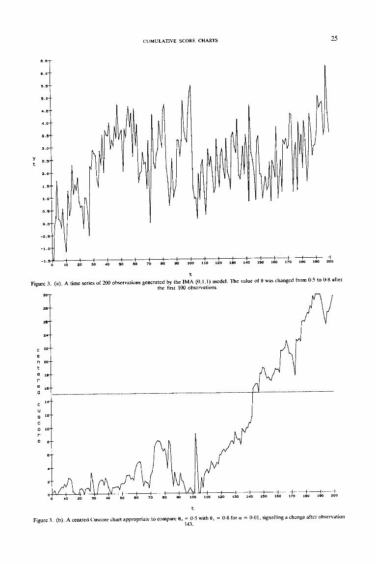
For illustration with the model (24) we used unit random normal deviates to generate the series of 200 values, shown in Figure 3(a) where the value of 8 was changed after 100 values from 0.5 to 0-8.

To illustrate the significance test, suppose B0 = 0.5, = 0-8 with u, = 1 and a = 0.01. We have h = ln(100)/0-3 = 15. Figure 3(b) shows the centred Cuscore statistic Q = -1/K2,z h,, where 6, is the EWMA of previous values with smoothing constant 8 = (0.5 + 0.8)/2 = 0.65, so that = 0.35. In this case the centred Cuscore for testing OO vs. O1 is equivalent to the test given by Bagshaw and J o h n ~ o n ' ~ to test a parameter change in an ARIMA model.

Although it is hard to see any difference in the series itself, the Q statistic does well in quickly reacting to the change and in indicating a significant change in 8 after observation 143.

DETECTING NON-STATIONARITY

One important industrial use of statistics is to maintain the industrial process in a state of statistical control, that is, in a stable or stationary state. To study statistical process control realistically, there- fore, we need a model which can not only represent the process in a stationary state but also in a non- stationary state. Now there is an infinite number of ways in which a process can be non-stationary. One important kind of non-stationarity is evidenced by a fluctuating series which exhibits a slow wandering drift away from target. The IMA model of equation (26) can represent such a drift and if in particular we suppose that at some time t = 0 the process has been adjusted to be on target by setting T = the subsequent behaviour of the process conditional on j 1 is obtained by summing equation (26). After writing A = 1 - 8, we then obtain the non- stationarity model in the form

I - I

Y , = T + a, + A C ~ ; (28) i= I

with

representing a process in a perfect state of control and the highly non-stationary random walk model

This model is of central importance to describe non-stationarity since it has the property,6 that the variogram or interval variance V , = V(y,+, - y,) increases linearly with m with the rate of increase depending on A, so that over a moderate range of m it might approximate a wide variety of non- stationary situations with the interval variance increased monotonically. Box and Kramer6 sug- gested as a general measure of non-stationarity the function G,,, = V,,/V, which shows by what factor the interval variance is inflated as rn increases. To give some idea of the degree of non-stationarity induced by the model (26) or equivalently (27) for a particular value of A they calculated the following intervals r)l required for the interval variance to double (for G,,, to take the value of 2).

A 0.05 0.10 0.20 0.50 1-00 m 762 181 42 6 2

From this and other evidence they concluded that values of A within the range 0.10 to 0.30 represented a degree of mild non-stationarity that might be of special interest to describe a number of industrial systems.

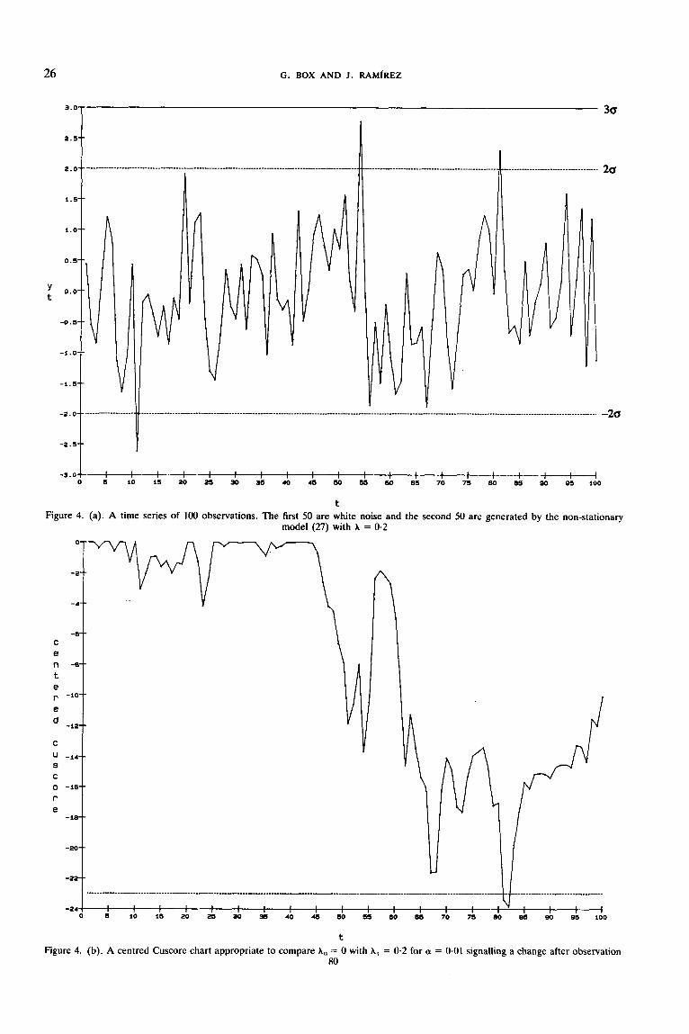
To detect non-stationarity we are looking for changes in the parameter A to some value greater than zero. For illustration we have plotted on Figure 4(a) a time series of 100 observations generated by equation (27) with u, = 1. For the first 50 observations A = 0 (0 = 1) and the deviations from target y, - T are thus white noise representing a process in a perfect state of statistical control. At time 50 the non-stationarity parameter was changed from A = 0 to A = 0.2, a change certainly not easy to see in the original plot and in particular no point falls outside the limits +3a,.

Figure 4(b) illustrates an appropriate test in which it is assumed that a, = 1, XO = 0, A l = 0.2, so that

= 0.1. Thus Q = -lOXti&, and with CY = 0.01, h = 4.6/0.2 = -23 we see that the chart signals a change after observation 80.

CONCLUSIONS

The main purpose of this paper is to point out that very sensitive sequential checks to monitor specific

CUMULATIVE SCORE CHARTS

30-

28--

20--

24--

c 22-- e n 20--

t e IB--

r

d 16--

c 14--

s 12--

U

25

.___ _ _ _ _ _ _ _ _ _ _ _ _ _ _ _ _ _ _ _ _ _ _ _ _ _ _ _ _ _ _ _ _ _ _ _ ~ _ _ _ _ _ _ _ _ _ _ _ _ _ _ _ _ _ _ _ _ _ _ _ _ _ _ _ _ ______ _ _ _ _ _ _ _ _ _ _ _ _ _ _ _ _______ _ _ ______ _ _ _ _ _ _ _ _ _ _ _ _ _ _ _ ~ _ _ _ _ _ _ _ _ _ _ _ _ _ _ _ _ _ _ _ _ _ _

I

! 1: 20 20 i o 20 20 40 I30 ,o , lo 1;o I$, I i O I 10 1 6 0 I d o , ; o o o -1 .5

t

Figure 3 . (a). A time series of 200 observations generated by the IMA (O, l , l ) model. The value of O was changed from 0.5 to 0.8 after the first 100 observations

26 G. BOX AND J . RAMfREZ

""T 3a

2a

Y t

-20

I -"I I I -3 .0 ! I I I I I 1 I I I 1 I ---f--.t--+-l

0 5 10 15 20 21 30 35 40 45 50 55 60 85 70 75 80 85 90 S5 100

t Figure 4. (a). A time series of 100 observations. The first 50 are white noise and the second 50 are generated by the non-stationary

model (27) with A = 0.2

t Figure 4. (b). A centred Cuscore chart appropriate to compare A,, = 0 with A, = 0.2 for a = 0.01 signalling a change after observation

80

CUMULATIVE SCORE CHARTS 27

feared deviations from a state of control can be derived easily.

A few of these are illustrated here, but the procedure is quite general.

Results can be presented in the form of suitable charts but we also have in mind that small process computers have also become common. These can be programmed to monitor simultaneously a number of possible discrepancies specific to a particular process, providing early warning and identification of sources of trouble.

REFERENCES

1. G. E. P. Box and G. M. Jenkins, ’Models for prediction and control: VI diagnostic checking’, Technical Report No. 99, University of Wisconsin-Madison, 1966.

2. G. E. P. Box and G. M. Jenkins, ‘Further contributions to adaptive optimization and control: simultaneous estimation of dynamics: non-zero costs’, Bulletin of the International Statisticaf Institute, 34th Session, Ottawa, 1963.

3. K. J. h r o m , Introduction to Stochastic Control. Mathematics in Science and Engineering Series, 70, Academic Press, 1970.

4. K. J. Astrom and B. Wittenmark, Computer Controlled Systems: Theory and Design, Prentice-Hall, New Jersey, 1984.

5. J. F. MacGregor, ‘Topics in the control of linear processes subject to stochastic disturbances’, Ph.D. Dissertation, University of Wisconsin-Madison, 1972.

6. G. E. P. Box and T. Kramer, ‘Statistical process control and automatic process control-a discussion, Technical Report 41, Center for Quality and Productivity Improvement, Uni- versity at Wisconsin, Madison, 1989; Technometrics, to appear.

7. G. E. P. Box, ‘Sampling and Bayes’ inference in scientific modelling and robustness’, J. Royal Stat. SOC., Series A , 143 (part 4), 383-430, (1980).

8. E. S. Page, ‘Continuous inspection schemes’, Biometrika, 41, 100-114 (1954).

9. G. A. Barnard, ‘Control charts and stochastic processes’, J. Royal Stat. SOC., Series B, 21, (2), 239-271 (1959).

10. N. L. Johnson, ‘A simple theoretical approach to cumulative sum control charts’, Journal of the American Statistical Association, 56, 835-840 (1961).

11. C. S. Van Dobben de Bruyn, Cumulative Sum Tests-Theory

and Practice, Hafner Publishing Co., New York, 1968. 12. B. M. Adams, C. Lowry and W. H. Woodall, ‘The use (and

misuse) of false alarms probabilities in control chart design’, submitted for publication, 1990.

13. G. E. P. Box and G. M. Jenkins, Time Series Analysis: Forecasting and Control, Holden-Day, San Francisco, 1970.

14. M. Bagshaw and R. Johnson, ‘Sequential procedures for detecting parameter changes in a time-series model’, Journal of the American Statistical Association, 72, 593-597 (1977).

Authors’ Biographies:

George Box is the Director of Research of the Center for Quality and Productivity Improvement at the University of Wisconsin-Madison. He has extensive industrial experience and is the originator of many widely used methods for product and process improvement, in particular the techniques of response surface methodology and evolutionary operation. He has made fundamental contributions to the theory and practice of statistically designed experiments, robust statistical methods, Bayesian methods and time series analysis and control. He has published over 150 papers and co-authored many books, including The Design and Analysis of Industrial Experiments, Statistical Methods in Research and Production, Time Series Analysis-Forecasting and Control, Bayesian Inference in Statistical Analysis, Evolutionary Operation, Statistics for Experimenters, and Empirical Model Building and Response Surfaces. He received Ph.D. and D.Sc degrees in mathematical statistics from the University of London, and an Honorary Doctorate from Carnegie Mellon University and the University of Rochester. He is a Fellow of the Royal Society and at the American Academy of Arts and Sci- ences.

Jod Ramirez is a practising statistician at Digital Equipment Corporation, where he consults in quality improvement initiatives and experimental design to manufacturing plants of the Semiconductor Operations. Before joining Digital he worked at the Statistical Laboratory and the Center for Quality and Productivity Improvement at the University of Wisconsin-Madison, where he conducted research on statistical process monitoring. He holds M.S. and Ph.D. in statistics from the University of Wisconsin-Madison.