CULTURAL PARTICLE SWARM OPTIMIZATION - CORE

CULTURAL PARTICLE SWARM

OPTIMIZATION

MOAYED DANESHYARI

Bachelor of Science

Electrical Engineering

Sharif University of Technology

Tehran, Iran

1995

Master of Science

Biomedical Engineering

Iran University of Science and Technology

Tehran, Iran

1998

Master of Science

Physics

Oklahoma State University

Stillwater, Oklahoma

2007

Submitted to the Faculty of the

Graduate College of the

Oklahoma State University

in partial fulfillment of

the requirements for

the Degree of

DOCTOR OF PHILOSOPHY

July 2010

ii

CULTURAL PARTICLE SWARM

OPTIMIZATION

Dissertation Approved:

Dean of the Graduate College

Dr. Gary G. Yen

Dissertation Adviser

Dr. Carl D. Latino

Dr. Louis G. Johnson

Dr. R. Russell Rhinehart

Dr. A. Gordon Emslie

iii

ACKNOWLEDGEMENTS

I would like to first thank my academic advisor, Professor Gary G. Yen, for his

guidance, support and especially patience with all ups and downs during the years of

studies that this dissertation was gradually constructed. If it were not with his flexibility

with my different situations and his providing me the freedom to fully experience all

aspects of academic research especially in the last two years, this academic research

could never be completed.

I would also like to extend my appreciation to the other committee members

whose guidance, comments and review of the research work were of great importance for

improving the quality of this document. My thanks also go to all my previous colleagues

at the Intelligent Systems and Control Laboratory at Oklahoma State University that

accompanied my progress throughout part of my research by offering me new ideas. I

should also mention my thankfulness to my colleagues in my current profession as

Assistant Professor at Elizabeth City State University whose help and flexibility to give

me more free time to focus on my Ph.D. research work was a great help.

Finally, I would like to express my gratitude for my parents, Farideh and Ahmad

and my sister Matin who have always supported me throughout my years of studies and

provided the understanding only possible although living far from me.

iv

Last, but not least, I would like to specially thank my family, my wife, Lily and

my little son, Ryan, for their understanding, help, support and providing appropriate

environment for me to work on my research during years of studying for doctorate

degree. If it were not her verbal and spiritual support and his innocence and happiness to

encourage me in working more, this study could never be accomplished.

Moayed Daneshyari

v

Table of Contents

Chapter Page

CHAPTER I

INTRODUCTION .......................................................................................................... 1

CHAPTER II

LITERATURE REVIEW ............................................................................................. 12

CHAPTER III

SOCIETTY AND CIVILIZAION FOR OPTIMIZATION .......................................... 29

3.1 Introduction ......................................................................................................... 29

3.2 Social-based Algorithm for Optimization ........................................................... 31

3.2.1 Proposed Modifications ............................................................................... 39

3.3 Simulation Results .............................................................................................. 42

3.4 Discussions ......................................................................................................... 44

CHAPTER IV

DIVERSITY-BASED INFORMATION EXCHANGE FOR PARTICLE SWARM

OPTIMIZATION .......................................................................................................... 46

4.1 Introduction ......................................................................................................... 46

4.2 Review of Related Work ..................................................................................... 48

4.3 Diversity-based Information Exchange among Swarms in PSO ........................ 54

4.4 Simulation Results .............................................................................................. 61

4.5 Discussions ......................................................................................................... 71

CHAPTER V

CULTURAL-BASED MULTIOBJECTIVE PARTICLE SWARM OPTIMIZATION

....................................................................................................................................... 73

5.1 Introduction ......................................................................................................... 73

5.2 Review of Literature ........................................................................................... 77

5.2.1 Related Works in Multiobjective PSO ......................................................... 77

5.2.2 Related Work in Cultural Algorithm for Multiobjective Optimization ....... 79

5.3 Cultural-based Multiobjective Particle Swarm Optimization ............................. 80

vi

5.3.1 Acceptance Function .................................................................................... 81

5.3.2 Belief Space ................................................................................................. 82

5.3.2.1 Situational Knowledge .......................................................................... 82

5.3.2.2 Normative Knowledge .......................................................................... 84

5.3.2.3 Topographical Knowledge .................................................................... 86

5.3.3 Influence Functions ...................................................................................... 89

5.3.3.1 Adapting Global Acceleration .............................................................. 89

5.3.3.2 Adapting Local Acceleration ................................................................ 91

5.3.3.3 Adapting Momentum ............................................................................ 93

5.3.3.4 Selection..................................................................................... 94

5.3.3.5 Selection ..................................................................................... 95

5.3.4 Global Archive ............................................................................................. 96

5.3.5 Time-decaying Mutation Operator .............................................................. 98

5.4 Comparative Study and Sensitivity Analysis ...................................................... 99

5.4.1 Comparison Experiment ............................................................................ 100

5.4.1.1 Parameter Settings .............................................................................. 100

5.4.1.2 Benchmark Test Functions ................................................................. 100

5.4.1.3 Qualitative Performance Comparisons ............................................... 102

5.4.1.4 Quantitative Performance Evaluations ............................................... 103

5.4.2 Sensitivity Analysis ................................................................................... 118

5.5 Discussions ....................................................................................................... 136

CHAPTER VI

CONSTRAINED CULTURAL-BASED OPTIMIZATION USING MULTIPLE

SWARM PSO WITH INTER-SWARM COMMUNICAION ................................... 139

6.1 Introduction ....................................................................................................... 139

6.2 Review of Literature ......................................................................................... 142

6.2.1 Related Work in Constrained PSO ............................................................ 142

6.2.2 Related Works in Cultural Algorithm for Constrained Optimization ........ 146

6.3 Cultural Constrained Optimization Using Multiple-Swarm PSO ..................... 147

6.3.1 Multi-Swarm Population Space ................................................................. 149

6.3.2 Acceptance Function .................................................................................. 150

vii

6.3.3 Belief Space ............................................................................................... 151

6.3.3.1 Normative Knowledge ........................................................................ 152

6.3.3.2 Spatial Knowledge .............................................................................. 153

6.3.3.3 Situational Knowledge ........................................................................ 155

6.3.3.4 Temporal Knowledge.......................................................................... 156

6.3.4 Influence Functions .................................................................................... 158

6.3.4.1 Selection ................................................................................... 158

6.3.4.2 Selection ................................................................................... 158

6.3.4.3 Selection................................................................................... 159

6.3.4.4 Inter-Swarm Communication Strategy ............................................... 159

6.4 Comparative Study............................................................................................ 162

6.4.1 Parameter Settings ..................................................................................... 162

6.4.2 Benchmark Test Functions ........................................................................ 163

6.4.3 Simulation Results ..................................................................................... 164

6.4.4 Convergence Graphs .................................................................................. 172

6.4.5 Algorithm Complexity ............................................................................... 178

6.4.6 Performance Comparison ........................................................................... 178

6.4.7 Sensitivity Analysis ................................................................................... 179

6.5 Discussions ....................................................................................................... 183

CHAPTER VII

DYNAMIC OPTIMIZATION USING CULTURAL-BASED PARTICLE SWARM

OPTIMIZATION ........................................................................................................ 186

7.1 Introduction ....................................................................................................... 186

7.2 Review of Literature ......................................................................................... 191

7.2.1 Related Work in Dynamic PSO ................................................................. 191

7.2.2 Related Works in Cultural Algorithm for Dynamic Optimization ............ 196

7.3 Cultural Particle Swarm for Dynamic Optimization ........................................ 196

7.3.1 Multi Swarm Population Space ................................................................. 198

7.3.2 Acceptance Function .................................................................................. 201

7.3.3 Belief Space ............................................................................................... 202

7.3.3.1 Situational Knowledge ........................................................................ 202

viii

7.3.3.2 Temporal Knowledge.......................................................................... 203

7.3.3.3 Domain Knowledge ............................................................................ 204

7.3.3.4 Normative Knowledge ........................................................................ 208

7.3.3.5 Spatial Knowledge .............................................................................. 212

7.3.4 Influence Functions .................................................................................... 215

7.3.4.1 pbest Selection .................................................................................... 215

7.3.4.2 sbest Selection ..................................................................................... 216

7.3.4.3 gbest Selection .................................................................................... 216

7.3.4.4 Diversity based Migration Driven by Change .................................... 216

7.4 Experimental Study ........................................................................................... 218

7.4.1 Benchmark Test Problems ......................................................................... 219

7.4.2 Comparison Algorithms ............................................................................. 220

7.4.3 Comparison Measure ................................................................................. 222

7.4.4 Simulation Results ..................................................................................... 222

7.5 Discussions ....................................................................................................... 232

CHAPTER VIII

CONCLUSION ........................................................................................................... 235

BIBLIOGRAPHY ........................................................................................................... 241

APPENDIX A

BENCHMARK TEST FUNCTIONS FOR MULTIOBJECTIVE OPTIMIZATION

PROBLEMS ............................................................................................................... 262

APPENDIX B

BENCHMARK TEST FUNCTIONS FOR CONSTRAINED OPTIMIZATION

PROBLEMS ............................................................................................................... 265

APPENDIX C

BENCHMARK TEST FUNCTIONS FOR DYNAMIC OPTIMIZATION

PROBLEMS ............................................................................................................... 289

ix

List of Figures

Figures Page

3.1 Flowchart for social-based single objective optimization 34

3.2 Flowchart for identifying leaders 35

3.3 Flowchart on how to migrate individuals 38

3.4 Pseudocode for individuality importance in intrasociety migration 40

3.5 Schema for Spring Design problem 43

3.6 Comparison for best objective function for proposed modifications 44

4.1 Ring and random sequential migration 56

4.2 Main algorithm for diversity-based multiple PSO 56

4.3 Schema of swarm neighborhood 59

4.4 Main algorithm for diversity-based multiple PSO with neighborhood 60

4.5 Benchmark function F1 with five peaks and four valleys 65

4.6 Final best particles for F1 65

4.7 Benchmark function F2 with 10 peaks 66


4.9 Benchmark function F3 with two peaks and one valley 67


4.11 Benchmark function F4 with five peaks 68


4.13 Benchmark function F5 with six peaks 69


5.1 Schema of particle’s movement in MOPSO 76

x

5.2 Pseudocode of the cultural MOPSO 81

5.3 Schema of the adopted cultural framework 82

5.4 Representation of situational knowledge 83

5.5 Schematic view of choosing the i-th element of situational knowledge 84

5.6 Representation of normative knowledge 85

5.7 Schema on how normative knowledge can be found and updated 88

5.8 Representation of knowledge in each cell 88

5.9 Example of cell representation 89

5.10 Schema of local grid for the personal archive 93

5.11 Method of selecting from topographical knowledge 96

5.12 selection procedure from personal archive 97

5.13 Pareto fronts comparison on test function ZDT1 105




5.17 Pareto fronts comparison on test function DTLZ5 109

5.18 Pareto fronts comparison on test function DTLZ6 110

5.19 Box plot of hypervolume indicator for all test function 111

5.20 Box plot for additive binary epsilon indicator on test function ZDT1 115




5.24 Box plot for additive binary epsilon indicator on test function DTLZ5 117

5.25 Box plot for additive binary epsilon indicator on test function DTLZ6 117

5.26 Sensitivity analyses with respect to minimum personal acceleration 123

5.27 Sensitivity analyses with respect to maximum personal acceleration 124

5.28 Sensitivity analyses with respect to minimum global acceleration 125

5.29 Sensitivity analyses with respect to maximum global acceleration 126

xi

5.30 Sensitivity analyses with respect to minimum momentum 127

5.31 Sensitivity analyses with respect to maximum momentum 128

5.32 Sensitivity analyses with respect to grid size 129

5.33 Sensitivity analyses with respect to population size 130

5.34 Sensitivity analyses with respect to mutation rate 131

6.1 Pseudocode of the cultural constrained particle swarm optimization 148

6.2 Schema of the cultural framework adopted 151

6.3 Representation for normative knowledge 152

6.4 The schema to represent how the spatial knowledge is computed 154

6.5 Representation of spatial knowledge for each particle 155

6.6 Representation for situational knowledge 156

6.7 Representation for temporal knowledge 157

6.8 Convergence graphs for problems 174




7.1 Pseudocode of the cultural-based dynamic PSO 198

7.2 Schema of the cultural framework adopted here 201

7.3 Representation for situational knowledge 203

7.4 Representation for temporal knowledge 203

7.5 Representation for the domain knowledge 206

7.6 Representation of normative knowledge 208

7.7 Representation for spatial knowledge 212

7.8 Sigmoid function to compute repulsion factor in spatial knowledge 213

7.9 Comparison of OEV as a function of elapsed iterations on function MP1 225

7.10 Comparison of OEV as a function of peak numbers on function MP1 225

xii

7.11 Comparison of OEV as a function of dimension on function MP1 226

xiii

List of Tables

Tables Page

3.1 Comparison of results for Spring Design problem 44

4.1 Results for optimal found and mean best objective for F1, F2, F3 and F5 70

4.2 Mean best objectives for F6, F7, F8, and F9 71

5.1 Parameter settings for all MOPSOs 101

5.2 Testing of the distribution of IH values using Mann-Whitney test 112

5.3 Testing of the distribution of using Mann-Whitney test 118

5.4 Parameter selection for sensitivity analysis 119

5.5 Statistical test to check sensitivity to minimum personal acceleration 132

5.6 Statistical test to check sensitivity to maximum personal acceleration 132

5.7 Statistical test to check sensitivity to minimum global acceleration 133

5.8 Statistical test to check sensitivity to maximum global acceleration 133

5.9 Statistical test to check sensitivity to minimum momentum 134

5.10 Statistical test to check sensitivity to maximum momentum 134

5.11 Statistical test to check sensitivity to grid size 135

5.12 Statistical test to check sensitivity to population size 135

5.13 Statistical test to check sensitivity to mutation rate 136

6.1 Parameter settings for cultural CPSO 162

6.2 Summary of 24 benchmark test functions 165

6.3 Error values for different FEs on problems 166


xiv



6.7 Number of function evaluations to achieve the fixed accuracy level, Success Rate,

Feasibility Rate, and Success Performance 171

6.8 Summary of statistical results found by cultural CPSO 173

6.9 Computational complexity 178

6.10 Comparison of cultural CPSO with the state-of-the-art constrained optimization

methods in terms of feasible rate 180

6.11 Comparison of cultural CPSO with the state-of-the-art constrained optimization

methods in terms of success rate 181

6.12 Sensitivity analysis with respect to personal acceleration 182

6.13 Sensitivity analysis with respect to swarm acceleration 183

6.14 Sensitivity analysis with respect to global acceleration 184

6.15 Sensitivity analysis with respect to rate of information exchange 185

7.1 Parameter settings for different paradigms 221

7.2 OEV index after 500,000 FEs on test problem MP1 224

7.3 OEV index after 500,000 FEs on test problem DF2 227





7.8 P-values using Mann-Whitney rank-sum test 231

7.9 OEV index after 50,000 FEs using default parameters 232

B.1 Data set for test problem 282

B.2 Data set for test problem 283

xv

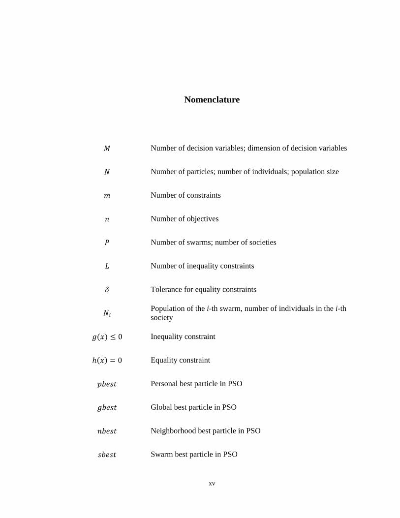
Nomenclature

Number of decision variables; dimension of decision variables

Number of particles; number of individuals; population size

Number of constraints

Number of objectives

Number of swarms; number of societies

Number of inequality constraints

Tolerance for equality constraints

Population of the i-th swarm, number of individuals in the i-th

society

Inequality constraint

Equality constraint

Personal best particle in PSO

Global best particle in PSO

Neighborhood best particle in PSO

Swarm best particle in PSO

xvi

Inequality constraint

Equality constraint

Personal acceleration in PSO

Global acceleration in PSO

Neighborhood acceleration in PSO

Swarm acceleration in PSO

Momentum in PSO

1

CHAPTER I

INTRODUCTION

Computational intelligence approaches based upon the psychosocial studies

inspired from either the human or animal society have been the subject of the emerging

research known as swarm intelligence. There has been some research in the area of

swarm intelligence focused on optimization in the spirit of the particle swarm [1], ant

colony system [2] and cultural algorithms [3]. While the population based heuristics

adopted in swarm intelligence do not mathematically guarantee to always find the global

optimum of the search space, they perform greatly well in different types of optimization

problems. Particle swarm optimization (PSO) is an imitation of the collaborative

behavior of the birds flying together with the means of their information exchange, while

ant colony is based on the fact that individual ants interact with each other through their

pheromone trails. Cultural algorithm (CA) is a dual inheritance system in which the

collective behavior of the population of individuals constructs the belief space which will

in turn be accessible to all individuals in the population space. Additionally, the

multinational algorithm [4] solves difficult multimodal optimization problems by using

heuristics imitating political interactions among nations.

2

In another heuristic, based on the relation between society and civilization [5] the

intersociety versus intrasociety relationship among the individuals facilitates on building

an optimization model. The whole population of individuals, called the civilization, is

clustered into different societies based on their Euclidean closeness of the individuals.

The performance of individuals will be a measure to decide which individuals are the

leaders of the society. The rest of the individuals are to follow them in a way to improve

themselves which leads to migration (intrasocitey interaction). From the civilization

viewpoint, the leaders of the societies will improve themselves by migrating toward the

best-performing leaders who are the civilization leaders (intersociety interaction). The

weakness of this paradigm is its lack on using existing information from all of the

individuals.

Particle swarm optimization is based on the changes of the positions and

velocities of the particles in a manner that optimizes a goal function. PSO has

demonstrated a promising performance for many optimization problems; yet its fast

convergence often leads to premature convergence in which the local optima of the goal

function are found instead of the global one. The tradeoff between fast convergence and

being trapped in local optima is even more critical in multimodal functions. In order to

escape from the local optima and avoid premature convergence, the search for global

optimum should be diverse. Many researchers have improved the performance of the

PSO by enhancing its ability with a more diverse search. Specifically, some have

proposed to use multiple swarms each running PSO, and then exchange information

3

among them. The weakness of these algorithms is their lack on considering a diverse list

of information to exchange, consequently premature convergence. Exchanging

information among clusters has also been adopted as an important design in several

computational methods. Distributed genetic algorithm [6] employs GA mechanism to

evolve several subpopulations in parallel. At regular intervals, migration among

subpopulations takes place. During the migration stage, a proportion of each

subpopulation is selected and sent to another subpopulation. The migrant individuals will

replace others based on a replacement policy.

Several population based heuristics have been developed to solve multiobjective

optimization problems (MOPs) among which multiobjective evolutionary algorithm

(MOEA) and multiobjective particle swarm optimization (MOPSO) are two popular

paradigms. Although there exist many research on single objective PSO suggesting

dynamic weights for the local and global acceleration, but most MOPSO researchers

assume that all particles should move with the identical momentum, local, and global

acceleration. To our best knowledge, there have not been any studies to consider a case in

which particles fly with different “personalized” weights for the momentum, local, and

global acceleration. Employing a personalized weight for each particle assigns a proper

jump contributing to the effectiveness of the overall performance of the algorithm. One

computational aspect is the difficulties of tuning proper value for the momentum,

personal, and global acceleration in MOPSO in order to attain the best results for

different test functions. From a biological point of view, work presented in [7] has also

4

shown that societies that can handle more complex tasks contain polymorphic

individuals. Polymorphism is a significant feature of social complexity that results in

differentiated individuals. The more differentiated the society, the easier it can handle

complex tasks. Differentiation applies in principal to complex societies of prokaryotic

cells, multicellular organisms, as well as to colonies of multicellular individuals such as

ants, wasps, bees, and so forth. The colony performance is improved if individuals

differentiate in order to specialize on particular tasks. As a result of differentiation,

individuals perform functions more efficiently. In their study it has been shown the

colony’s ability to higher cooperative activity when tackling tasks is a direct consequence

of differentiation among other factors.

There are few studies in the MOPSO research area that have tackled the issue of

variable momentum for the particles although in all of them momentum is identical for all

particles at a specific iteration. Some MOPSO paradigms have proposed simple strategies

to adapt the momentum by simply decreasing the momentum throughout swarming while

other MOPSO algorithms choose a random value for momentum at every iteration. To

the best knowledge of the author, there is no noticeable study in MOPSO on adapting

personalized dynamic momentum and acceleration based upon the need for the particles

to exploration or exploitation.

Constrained optimization problem is another area that has been solved using

population based paradigms during the last two decades. Swarm-based algorithms have

recently been developed to handle constraints in these type of problems. Although there

5

are few research studies on PSO to solve constrained optimization problems, none of

these studies adopt the information from all particles to perform communication within

PSO in order to share common interest and to act synchronously. When particles share

their information through communication with each other, they will be able to efficiently

handle the constraints and optimize the objective function. From a sociological point of

view, study has shown that human societies will migrate from one place to another in

order to handle their own life constraints and limitations as well as to reach a better

economical, social, or political life [8]. People living in different societies migrate in spite

of the different value systems and cultural differences. Indeed the cultural belief is an

important factor affecting the issues underlying the migration phenomena [9]. On the

other hand, finding the appropriate information for communication within swarm can be

computationally expensive. One computational aspect is the difficulties of finding the

appropriate information to communicate within PSO in order to be able to simultaneously

better handle the constraints and optimize the objective function.

The optimum solution for many real-world optimization problems changes over

time. In such cases known as dynamic optimization problems, the heuristics should track

the change as soon as it happens and responds promptly. For example, in job scheduling

problems new jobs arrive or machines may break down during operations results a need

for dynamic job schedules to accommodate the changes over time [10]. In another

example, dynamic portfolio problem, the goal is to obtain an optimal allocation of assets

to maximize profit and minimize investment risk [11].

6

There are four major categories of uncertainties that have been dealt with using

population based evolutionary approaches: noise in the fitness function, perturbations in

the design variables, approximation in the fitness function, and dynamism in optimal

solutions [12]. While noise and approximation bring uncertainty in the objective function,

perturbation introduces uncertainty in the decision space. The source of change can be

because of the possible change in the objective function, constraints, environmental

parameters, or problem representations during optimization process. These changes may

affect the height, width, or location of optimum solution or a combination of these three

parts [13].

The application of PSO to dynamic optimization problems has been studied by

various researchers. There are some issues with the PSO mechanism that needs to be

addressed. Maintaining outdated memory is one issue in dynamic optimization problems.

When a problem changes, a previously good solution stored as neighborhood or personal

best may no longer be good, and will mislead the swarm towards false optima. Diversity

loss is another problem in which population normally collapses around the best solution.

In dynamic optimization, the partially converged population after a change is detected

should quickly re-diversify, find the new optimum and re-converge [10]. A number of

adaptations have been applied to PSO in order to solve these difficulties. In general, a

good evolutionary heuristic to solve DOPs should reuse as much information as possible

from previous iterations to increase the optimization search. Among the researches

performed in dynamic PSO none of these studies exploits information from all particles

7

to perform re-diversification through migration and repulsion. When particles share their

information through migration process, they will be able to quickly re-diversify and move

efficiently towards new optimum by re-converging around it. In order to construct the

environment required for this re-divergence and re-convergence, we need to establish

groundwork to assist us to utilize this information. The major groundwork is the belief

space of cultural algorithm assisting the particles in an organized informational manner to

locate the necessary information.

Discussed in psychosocial texts, attitudinal similarity is a leading factor to

attraction among individuals while dissimilarity leads to repulsion in interpersonal

relationship [14], as a result people often diverge from members of other social groups by

selecting different cultural attitudes or behaviors [15]. Indeed different cultural beliefs

lead to repulsion and increase the possibilities of divergence in ideas and in turn open up

the doors to new opportunities.

One challenge is the difficulty to find the appropriate information to use so that it

can be relied on for a quick re-diversification when a change happens in the environment.

Using many concepts from the cultural algorithm, such as spatial knowledge, temporal

knowledge, domain knowledge, normative knowledge and situational knowledge, the

information will be organized competently and successfully in order to adopt in several

steps of the PSO’s updating mechanism in addition to re-diversification and repulsion

among swarms. The special re-diversification problem to deal with the change in

dynamic is an important task that can be solved more efficiently when we have access to

8

the knowledge throughout the search process that is performed by the cultural algorithm

as the computational framework.

The remaining structure of this dissertation is as following. In Chapter II, a

comprehensive literature survey is performed on related computational intelligence

paradigms to prepare for the following chapters. Chapter III firstly elaborates on a

paradigm based upon the intrasociety and intersociety interaction in order to simulate an

algorithm to solve single objective optimization problems. Next the proposed

modifications to this social-based heuristics will be introduced. This proposal has two

aspects: one is based upon the idea of adopting information from all individuals in the

society (i.e., not only the best performing individuals). The second proposal is based on

the fact that different societies have different collective behavior. Politically speaking, the

collective behavior of the societies have been quantified into a measure called the liberty

rate. In the real sociological context, individuals in a democratic society will have more

flexibility and freedom to choose a better environment to live. In contrast, individuals in a

dictatorship society will suppress the politically environmental change. While individuals

in a liberal society can freely move to be closer to the leaders, individual in a less liberal

society will have restriction to move near the leaders. Hence the higher liberty rate a

society has, the more flexibility an individual in such society can move. At the end of this

chapter, simulation result for a real world mechanical problem is used to test the

performance of two proposed modifications.

In Chapter IV, a heuristic is proposed to diversify the search space using a novel

9

three-level particle swarm optimization in a multiple swarm population space. The PSO

mechanism is customized to incorporate three levels of searching process. In the lowest

level, particles follow the best behaving particle in their own swarm; in next level,

particles follow the best performing particle in the neighboring swarms, and finally in the

highest level, particles track the whole population’s best behaving particle. A novel

algorithm is proposed to define the neighboring swarms based upon the closeness

between representatives of each pair of swarms. After a specified number of iterations,

the swarms communicate with each other. Each swarm assembles two lists, a sending list

and a replacement list. To prepare these two sets of particles, diversity measure is

considered as the primary goal instead of the performance of the particles alone. When

particles are approaching the local optima, several of them will have similar positional

information. This similar redundant information will be replaced by particles from other

swarms to diversify the search space. At the end of this chapter, the simulated study is

tested to solve benchmark multimodal optimization problems which demonstrate

efficiency of the proposed heuristic and its potential to solve difficult optimization

problems.

Chapter V proposes an innovative algorithm adopting the cultural information that

exists in the belief space to adjust flight parameters of multiobjective particle swarm

optimization (MOPSO) such as personal acceleration, global acceleration, and

momentum. A belief space has been constructed containing three sections of knowledge

as the groundwork to perform MOPSO and adapt the parameters. Every particle in

10

MOPSO will use its own adapted momentum and acceleration (local and global) at every

iteration to approach the Pareto front. Cultural algorithm provides the required

groundwork enabling us to employ the information stored in different belief space

efficiently and effectively. The proposed cultural MOPSO is then evaluated against the

state-of-the-art MOPSO models, showing very competitive and well performing

outcome. Finally a comprehensive sensitivity analysis has been performed for the cultural

MOPSO with respect to its tuning parameters.

In Chapter VI, a novel heuristics is proposed based upon the information

extracted from belief space to facilitate the inter-swarm communication among multiple

swarms in particle swarm optimization to solve constrained optimization problems. The

cultural computational framework is to find the leading particles in the personal level,

swarm level, and global level. Every particle will move using a three-level flight

mechanism and then particles divide into several swarms and inter-swarm

communication takes place to share the information. The performance of the proposed

cultural constrained particle swarm optimization (CPSO) has been compared against ten

state-of-the-art constrained optimization paradigms on 24 benchmark test problems. The

comprehensive simulation results demonstrate cultural CPSO to be very effective and

efficient.

Chapter VII proposes an innovative computational framework according to

cultural algorithm to solve dynamic optimization problems using knowledge stored in the

belief space in order to re-diversify and repel the population right after a change takes

11

place in the dynamic of the problem. Thus the algorithm can comfortably compute the

repulsion factor for each particle and locate the leading particles in the personal level,

swarm level and global level. Each particle in the proposed cultural-based dynamic PSO

will fly through a mechanism of three level flight incorporated with a repulsion factor.

After a change takes place, particles regroup into several swarms and a diversity-based

migration among swarms along with repulsive mechanism implemented in repulsion

factor will take place to increase the diversity as quickly as possible.

Finally, Chapter VIII discusses the concluding remarks on how swarm, culture,

and society help in solving single objective, multiobjective, constrained, and dynamic

optimization problems. The suggestions of the future work of this study are also proposed

in this chapter.

12

CHAPTER II

LITERATURE REVIEW

In this chapter, we briefly review the related work that will assist in understanding

the background concepts required for this dissertation. Population based computational

intelligence heuristics has extensively evolved from natural evolutionary-based Genetic

Algorithms (GA) [16-17] over decades of research work. Computational intelligence

approaches based upon the psychosocial behavior inspired from either human or animal

society have been the subject of the emerging research for a decade. Some concepts

borrowed from sociology have shown great improvements in the performance of

computational methods. Migration of individuals between concurrent evolving

populations has shown its potential to improve the genetic algorithms mechanism [18]. In

distributed GA [6] the sociologically inspired concept of communication shows great

improvement in the performance of GA. The population is divided into several

subpopulations each evolving an independently GA while at regular time intervals, these

GAs communicate with each other.

Sociological researchers have constructed models to mimic the behavior of human

and animal societies. Heppner and Grenander studied synchronization in groups of small

birds like pigeons developing a flocking heuristics based upon the social interactions such

13

as attraction to a roost, attraction to flockmates and preserving the velocity [19].

Deneubourg and Goss has shown that the interaction between the individuals and their

environment produces different collective patterns on decision making process by

introducing a mathematical model [20] which is naturally observed to be essential in the

schools of fishes, flocks of birds, groups of mammals, and many other social aggregates.

Millonas proposed a model of the collective behavior of a large number of locally

acting organisms [21] in which organisms move probabilistically between local cells in

space, but with different weights. The evolution and the flow of the organisms construct

the collective behavior of the group. This model could successfully analyze movements

of ants as swarming organism. Reynolds developed a computer animator of a simulated

bird based upon the local perception of the dynamic environment, the laws of simulated

physics ruling its motion, and a set of simulated behaviors [22].

Akhtar et al. proposes a socio-behavioral simulated model [23] based upon the

concept that the behavior of an individual changes and improves due to social interaction

with the society leaders who are identified using a Pareto rank scheme. On the other

hand, the leaders of all societies themselves improve their own behavior which leads to a

better civilization. Ursem introduced multinational evolutionary algorithm based on the

relationship between different nations and their political interaction in order to optimize a

profit function [4]. Ray and Liew adopted the intersociety and intrasociety relationship

among the individuals and the leaders to optimize the single objective optimization

problem [5]. The whole population, clustered into several groups, evolves in two stages.

14

Individuals within group follow the group’s best performing individual, and in the whole

population, the very best performing individual leads all groups’ leaders. Ursem

elaborates the idea of sharing among agents in a social entity as a means of maintaining

multiple peaks in multimodal optimization problems [24].

Deneubourg and coauthors proposed a probabilistic model to explain behavior of

ants as social agents [25] which was then followed by Goss et al. showing how sharing

information among ants which was done by laying trail and following it could help to

solve foraging problem in their societies [26]. Inspired by their research, Dorigo et al.

introduced a new computational paradigm, Ant Colony Optimization (ACO) model, that

could be adopted to solve engineering optimization problems. ACO’s main characteristic

was a positive feedback for rapid discovery of good solution of optimization problem, a

distributed computation to avoid premature convergence, and a greedy heuristic to find

acceptable solution in the early stages of the search process [2, 27]. The ACO model has

been successfully applied to symmetric and asymmetric Travelling Salesman Problem

(TSP) as a classical difficult combinatorial optimization problem [28-29], quadratic

assignment problem [30], adaptive routing [31], job-scheduling problem [2]. Sahin et al.

reported applying the ant-based swarm algorithm on forming different patterns through

interaction among mobile robots [32].

Kennedy and Eberhart introduced the particle swarm optimization (PSO), an

algorithm based on imitating behavior of flocking birds. It mimics grouping of birds as

particles, their random movement, and regrouping them again to generate a model so that

15

it can solve engineering optimization problems [1, 33]. Particles are known with their

positions and velocities and can be updated using:

, (2.1)

,

where is the velocity of the particle, is the position of the particle, is the best

position of each particle ever experienced, and is the best position among all

particles. and are random numbers uniformly generated in the range of . , ,

and are personal, social, and momentum coefficients [34] that are predefined constant

values. The movement of the particles has been analyzed to understand the mechanism

underlying the PSO and its relation to other population based heuristics [35]. The analysis

of the particles’ trajectory while moving [36] has led to a generalized model of the

algorithm, containing a set of coefficients to control the system's convergence tendencies.

The effects of various population structure and topologies on the performance of particle

swarm algorithm have shown that von Neumann configuration consistently outperforms

other types of topological configurations of particles’ neighborhood [37-39].

Several versions of PSO have been developed. Discrete PSO was introduced [40]

operating on discrete binary variables whose trajectories are defined as changes in the

probability that a coordinate will take on a zero or one value. Comparing with GA on

some multimodal optimization problems, discrete PSO showed competitive results [41-

16

42]. A modified PSO using constriction factor [43] performed well comparing with the

original PSO. Particle swarms are also developed to track and optimize dynamic

landscape systems [44]. Particle swarm optimization has also been modified to perform

permutation optimization problems such as N-queens problem [45] by defining particles

as permutations of a group of unique values and updating velocity based upon the

similarity of two particles. The permutation of the particles change with a random rate

defined by their velocities.

Clustering population into several swarms has been extensively studied.

Stereotyping of the particles is investigated [46] in which substitution of cluster centers

for shows better performance of the PSO suggesting that PSO is more effective

when individuals are attracted toward the center of their own clusters. Al-Kazemi and

Mohan divided the population into two sets at any given time, one set moving to the

while another moving in opposite direction by selecting appropriate fixed values

for in each set [47]. After some iterations, if the would not improve,

then the particles would switch their group. Baskar and Suganthan introduced a

concurrent PSO consisting two swarms in order to search concurrently for a solution

along with frequent passing of information, the of two swarms [48]. After each

exchange, the two swarms had to track the better found. One of the swarms was

using regular PSO while the other was using the Fitness-to-Distance ratio PSO [49].

Their approach improved the performance over both methods in solving single objective

optimization problems. El-Abd and Kamel added a two-way flow of information between

17

two swarms improving its performance [50]. In their algorithm, when exchanging the

best particle between two swarms, this particle is used to replace the worst particle in

another swarm. The two swarms perform a fixed number of iterations, and then the best

particles inside each swarm will replace the worst particles in the other swarm only if

they have a better fitness. This makes it possible for both swarms to exchange new

information from the other swarm’s experience. Krohling et al. proposed co-evolutionary

PSO in which two populations of PSO are involved [51]. One PSO runs for a specified

number of iterations while the other remains static and serves as its environment. At the

end of such period, values obtained in previous cycles have to be re-evaluated

according to the new environment before starting evolution.

Particle swarm optimization has been widely applied for multiobjective

optimization problems (MOPs) called multiobjective particle swarm optimization

(MOPSO) to find a diverse set of potential solutions, known as Pareto front. There have

been several algorithms to extend PSO to handle diversity issue in MOPs. Parspopoulos

et al. [52] introduced vector evaluated particle swarm optimizer (VEPSO) to solve

multiobjective problems. A VEPSO is a multi-swarm variant of PSO in which each

swarm is evaluated using only one of the objective functions of the problem under

consideration, and the information it possesses for this objective function is

communicated to the other swarms through the exchange of their best experience. In

VEPSO, the velocity of the particles in each swarm is updated using the best previous

position, , of another selected swarm. Selection of this swarm in the migration

18

scheme can be either random or in a sequential order. Ray and Liew [53] used Pareto

dominance and combined concepts of evolutionary techniques with the particle swarm.

This algorithm uses crowding distance to preserve diversity. Hu and Eberhart [54] in their

dynamic neighborhood PSO proposed an algorithm to optimize only one objective at a

time. The algorithm may be sensitive to the optimizing order of objective functions.

Fieldsend and Singh [55] proposed an approach in which they used an unconstrained elite

archive to store the nondominated individuals found along the search process. The

archive interacts with the primary population in order to define local guides. Mostaghim

and Teich [56] introduced a sigma method in which the best local guides for each particle

are adopted to improve the convergence and diversity of the PSO. Li [57] adopted the

main idea from NSGA-II into the PSO algorithm. Coello Coello et al. [58], on the other

hand proposed an algorithm using a repository for the nondominated particles along with

adaptive grid to select the global best of PSO. The algorithms proposed to solve MOPs

using PSO are based upon promoting the nondominated particles at any given time, not

exploiting the information of all particles in the population.

Many MOPSO paradigms are focused on the methods of selecting global best [53,

55-56, 58-64], or personal best [65]. Most MOPSOs adopt constant value for momentum

and accelerations; however some MOPSOs use some simple dynamic to change the

parameters. Indeed, one of the difficulties of the PSO and/or MOPSO is to deal with

tuning the right value for the momentum, personal and global acceleration in order to get

the best results for different test functions. Hu and Eberhart [54] in their dynamic

19

neighborhood MOPSO model and also Hu et al. [66] in the MOPSO with extended

memory adopted a random number on the range (0.5,1) as the varying momentum.

However both personal and global acceleration are constant values. Sierra and Coello

Coello [62] in their crowding and -dominance based MOPSO used random value at the

range (0.1,0.5) for the momentum and random values at the range (1.5,2.0) for the

personal and global acceleration. They adopted this scheme to bypass the difficulties of

fine tuning of these parameters for each test function.

Zhang et al. [64] introduced intelligent MOPSO based upon Agent-Environment-

Rules model of artificial life. In their model, along with adopting some immunity clonal

operator, the momentum was decreased linearly from 0.6 to 0.2, but the personal and

global acceleration remained constant. Li [67] proposed an MOPSO based upon max-min

fitness function. In his model, while the personal and global acceleration were set

constant, the momentum was gradually decreased from 1.0 to 0.4. Zhang et al. [68]

adopted a linearly-decreasing momentum from 0.8 to 0.4 for their MOPSO algorithm.

However the personal and global acceleration were kept fixed. Mahfouf et al. [69]

introduced adaptive weighted MOPSO in which they included adaptive momentum and

acceleration. Using comparison study with other well-behaved algorithms, they

demonstrated that the MOPSO search capability is enhanced by adding this adaptation.

Ho et al. [63] noted the possible problem of selecting personal and global acceleration

independently and randomly. He mentioned because of its stochastic nature they may

both be too large or too small. In the former case, both personal and global experiences

20

are overused and as a result the particle will be driven too far away from the optimum.

For the latter case, both personal and global experiences are not fully used and as a result

the convergence speed of the algorithm is reduced. They used sociobiological activity

such as hunting to assure that individuals balance between the weight of their own

knowledge and the group’s collective knowledge. In other words, they mentioned that the

personal and global acceleration are somehow related to each other. When one

acceleration is large, the other one should be small, and vice versa. Using this concept,

they modified the main equation of PSO, Equation (2.1) to include a dependent

acceleration and momentum [63].

Particle swarm optimization algorithms have been successfully developed to solve

constrained optimization problems. Hu and Eberhart generated particles in PSO until the

algorithm could find at least one particle in the feasible region and then adopted it to find

best personal and global particles [70]. Parsopoulos and Vrahatis used a dynamic multi-

stage penalty function to handle the constraints [71]. The penalty function consisted of

weighted sum of all constraints violation with each constraint having a dynamic exponent

and a multi-stage dynamic coefficient. A comparison of preserving feasible solution

method [70] and dynamic penalty function [71] demonstrated that the convergence rate

for dynamic penalty function algorithm was faster than that of feasible solution method

[72].

Hu et al. modified the PSO mechanism to solve constrained optimization

problems. PSO starts with a group of feasible solutions and a feasibility function is used

21

to check if the newly explored solutions satisfy all the constraints. Only feasible solutions

are kept in the memory [73]. Linearly constrained optimization problems are the basis for

a modified version of PSO in which the movement of the particles in the vector space is

mathematically guaranteed by the velocity and position update mechanism to always find

at least a local optimum [74]. In the constrained PSO, particles that satisfy constraints

move to optimize the objective function while particles that violate constraints move in

order to satisfy the constraints [75].

Krohling and Coelho adopted Gaussian distribution instead of uniform

distribution for the personal and global term random weights of the PSO mechanism to

solve constrained optimization problems formulated as min-max problems. They used

two populations of the PSO simultaneously, first PSO focuses on evolving the variable

vector while the vector of Lagrangian multiplier is kept frozen, and the second PSO is to

concentrate on evolving the Lagrangian multiplier while the first population is

maintained frozen. The use of normal distribution for the stochastic parameters of the

PSO seems to provide a good compromise between the probability of having a large

number of small amplitude around the current points, i.e., fine-tuning, and small

probability of having large amplitudes, that may cause the particles to move away from

the current points and escape from the local optima [76].

In master-slave PSO [77], master swarm is to optimize objective function while

slave swarm is focused on constraint feasibility. Particles in the master swarm only fly

toward the current better particles in the feasible region, and they will not fly toward

22

current better particles in the infeasible region. The slave swarm is responsible for

searching feasible particles by flying through the infeasible region. Particles in slave

swarm only fly toward current better particles in the infeasible region, and they will not

fly toward current better particles in the feasible region. The feasible/infeasible leaders

from swarm will then be communicated to lead the other swarm. By exchanging flight

information between swarms, algorithm can explore a wider solution space.

Zheng et al. adopted an approach that congregates neighboring particles in the

PSO to form multiple swarms in order to explore isolated, long and narrow feasible space

[78]. They also applied a dynamic mutation operator with dynamic mutation rate to

enhance flight of particles to feasible region more frequently. For constraint handling a

penalty function has been adopted as to how far the infeasible particle is located from the

feasible region. Saber et al. [79] introduced a version of PSO for constrained

optimization problems. In their version of PSO, the velocity update mechanism uses a

sufficient number of promising vectors to reduce randomness for better convergence. The

coefficient velocity in the positional update equation is a dynamic rate depending on the

error and iteration. They also reinitialized the idle particles if there are particles that are

not improving for some iterations. Li et al. [80] proposed dual PSO with stochastic

ranking to handle the constraints. One regular PSO evolves simultaneously along with a

genetic PSO, a discrete version of PSO including a reproduction operator. The better of

the two positions generated by these two PSOs is then selected as the updated position.

Flores-Mendoza and Mezura-Montes [81] used Pareto dominance concept for constraint

23

handling technique on a bi-objective space, with one objective being sum of the

inequality violation constraints and the second objective being sum of the equality

violation constraints in order to promote better approach to feasible region. They also

adopted a decaying parameter control for constriction factor and global acceleration of

the PSO to prevent the premature convergence and to advance the exploration of the

search space. Ting et al. [82] introduced a hybrid heuristic consisting PSO and genetic

algorithm to tackle constraint optimization problem of load flow algorithm. They adopted

two-point crossover, mutation, and roulette-wheel selection from genetic algorithms

along with the regular PSO to generate the new population space. Liu et al. [83]

incorporated discrete genetic PSO with differential evolution (DE) to enhance the search

process in which both genetic PSO and DE update the position of the individual at every

generation. The better position will then be selected.

Particle swarm optimization algorithms have been effectively developed to solve

dynamic optimization problems (DOP) as well. Carlisle and Dozier [84] adjusted PSO

mechanism to prevent making position/velocity decision according to the outdated

memory by periodic resetting. Particles periodically replace their pbest vector with their

current position, forgetting their past experiences. Eberhart and Shi [44] proposed that for

small perturbation, the initialization of the swarm can start from old population, while

large perturbation needs re-initialization. In detection and response paradigm [85] gbest

and the second global best are evaluated to detect changes, then the positions of all

particles are re-randomized to respond to the change. Charged swarm avoids collision

24

among particles based upon the force between electric charges which is inversely

proportional to distance squared [86]. Atomic PSO [87] and quantum PSO [88] follow

the structure of the chemical atom including a cloud of electrons randomly orbiting with a

specific radius around the nucleolus.

An anti-convergence operator [89] assists interaction among swarms. Also an

excluding operation defines a radius to include the best solution of the swarm. These

close swarms compete with each other in order to promote diversity. The winner, the

swarm with the best function value at its swarm attractor, will remain, while the loser will

be re-initialized in the search space [89]. Swarms birth and death [90] was proposed by

allowing multiple swarms to regulate their size by bringing new swarms to existence, or

diminishing redundant swarms. This dynamic swarm size can be an alternative for anti-

convergence and exclusion operators in the PSO mechanism.

In partitioned hierarchical PSO for dynamic optimization problems [91], the

population is partitioned into some tree-form sub-hierarchies for a limited number of

iterations after a change is detected. These sub-hierarchies continue to independently

search for the optimum, resulting a wider spread-out of the search process after the

change has occurred. The topmost level of tree-form hierarchies which contain the

current best particle does not change, but all lower sub-hierarchies (sub-swarms) re-

initialize the position and velocity and reset their personal best positions. These sub-

hierarchies are rejoined again after a predefined number of iterations.

25

By adopting dynamic macro-mutation operator [92], PSO is able to maintain the

diversity throughout the search process in order to solve DOPs. Every coordinate of each

particle will undergo an independent mutation with a dynamic probability which possess

its highest value when the change occurs in the dynamic landscape and gradually

decreases till the next change takes place. The unified PSO in which the exploration and

exploitation term of the PSO mechanism are unified into a unification factor has also

been adopted for solving DOPs [93]. Zhang et al. [94] proposed a direct relation between

the inertia weight of the particle and the change. In their model, the new gbest and pbest

for each particle affect the inertia weight of the particle whenever a change in gbest or

pbest occurs. Pan et al. [95] modified the PSO paradigm using a probability based

movement of particles based upon the concept of energy change probability in Simulated

Annealing (SA). The particle will move to the next position computed through traditional

PSO heuristics only with a specific probability that exponentially depends on the

difference between the objective values of the current and next iterations.

In species based PSO [96], the population is divided into some swarms, each

surrounding a dominating particle called seed identified from the objective function

values of the entire population. The new seed should not fall within the predefined radius

of all previously found seeds in order to promote diversity. The seeds are then selected as

the neighborhood best for different swarms. In multi-strategy ensemble PSO [97],

particles are divided into two sections, part I uses a Gaussian local search to quickly seek

global optimum in the current environment, while part II uses differential mutation to

26

explore the search space. The position of particles in part II do not follow the traditional

PSO mechanism, instead each particle in part II is determined by the particle in part I

through a mutation strategy.

Liu et al. [98] introduced a modified PSO to solve DOPs in which many

compound particles exist. Each compound particle includes three single particles

equilaterally distanced from each other in a triangular shape. A special reflection scheme

is proposed to explore the search space more comprehensively in which the position of

the worst particle among three in the compound will be replaced with the reflected one.

In each compound particle, after reflection is performed, a representative among these

three particles is probabilistically chosen based upon the objective function values and

distance from other two member particles. The representative member particles will then

participate in PSO update mechanism. The two non-representative particles will also

move in the same distance/direction as representative particle has been moved in order to

preserve the valuable information.

Recently a computational framework has been developed by Reynolds known as

cultural algorithm (CA) based upon a dual inheritance system where information exists at

two different levels: population level and the belief level [3]. Culture is defined as storage

of information which does not depend on the individuals who generated and can be

potentially accessed by all society members [3]. CA is an adaptive evolutionary

computation method which is derived by cultural evolution and learning in agent-based

societies [3, 99]. CA consists of evolving agents whose experiences are gathered into a

27

belief space consisting of various forms of symbolic knowledge. CA has shown its ability

to solve different types of problems [3, 99-107] among which CAEP (cultural algorithm

along with evolutionary programming) has shown successful results in solving MOPs

[107]. Researchers have identified five basic sections of knowledge stored in belief space

based upon the literature in cognitive science and semiotics: situational knowledge,

normative knowledge, topographical knowledge [105], domain knowledge, and history

knowledge [106]. Situational knowledge is a set of exemplary individuals useful for

experiences of all individuals. Situational knowledge guides all individuals to move

toward the exemplar individuals. Normative knowledge consists a set of promising

ranges. Normative knowledge provides standard guiding principle within which

individual adjustments can be made. Individuals jump into the good range using

normative knowledge. Topographical or spatial knowledge keeps track of the best

individuals which have been found so far in the promising region. Topographical

knowledge leads all individuals toward the best performing cells in the search space

[105]. Domain knowledge adopts information about the problem domain to lead the

search. Domain knowledge about landscape contour and its related parameters guides the

search process. Historical or temporal knowledge keeps track of the history of the search

process and records key events in the search. It might be either a considerable move in

the search space or a discovery of landscape change. Individuals use the history

knowledge for guidance in selecting a move direction. Domain knowledge and history

knowledge are useful on dynamic landscape problems [106]. The knowledge can swarm

28

between different sections of belief space [108-110] which in turn affect the swarming of

population.

Becerra and Coello Coello [104] proposed cultured differential evolution for

constrained optimization. The population space in their study was differential evolution

(DE) while the belief space consist of situational, topographical, normative, and history

knowledge. The variation operator in DE was influenced by the knowledge source of

belief space. Yuan et al. [111] introduced chaotic hybrid cultural algorithm for

constrained optimization in which population space as DE and belief space including

normative and situational knowledge. They incorporated a logistic map function for

better convergence of DE to use its chaotic sequence. Tang and Li [112] proposed a

cultured genetic algorithm for constrained optimization problems by introducing a triple

space cultural algorithm. The triple space includes belief space, population space in

addition with anti-culture population consisting individuals disobeying the guidance of

the belief space, and going away from the belief space guided individuals. The effect of

disobeying behavior enhanced by some mutation operations makes the algorithm faster

and less risky for premature convergence, by awarding the most successful individuals

and punishing the unsuccessful population.

29

CHAPTER III

SOCIETTY AND CIVILIZAION FOR OPTIMIZATION

3.1 Introduction

Computational intelligence approaches based upon the psychosocial behavior

inspired from either the human or animal society have been the subject of the emerging

research for less than a decade. There has been some research in this area focused on

optimization in the spirit of the particle swarm intelligence [1] or ant colony system [2].

Particle swarm optimization is an imitation of the collaborative behavior of the birds

flying together with the means of information exchange, while ant colony is based on the

fact that individual ants interact with each other through their pheromone trails.

Additionally, Ursem [4] introduced another ideas based on the relationship between

different nations and how to interact between the countries in order to optimize a profit

function. More recently, in an attempt to mimic the interactional behavior between

societies and within civilization, social algorithm had been proposed [5, 113]. Social

algorithm adopts the intersociety and intrasociety relationship among the individuals and

the leaders to optimize the single objective optimization problem. The whole population

of individuals, called the civilization, is clustered into different societies based on the

30

Euclidean closeness of the individuals. The performance of individuals will be a measure

to decide which individuals are the leaders of the society. The rest of the individuals are

to follow them in a way to improve themselves which leads to migration (intrasocitey

interaction). From the civilization viewpoint, the leaders of the societies will improve

themselves by migrating to the best-performing leaders who are the civilization leaders

(intersociety interaction) [114-115].

Ray and Liew have successfully demonstrated the performance of their model in

single objective optimization problems [5]. Their model seems to be an alternative

competitive paradigm to particle swarm heuristics. What was used in their model is

mostly by throwing the information of the non-leader individuals away and replacing

with those of the corresponding leaders. What is proposed in this chapter involves two

aspects. Firstly, using the information of the individual, individual’s talent is computed

which equips each individual with different ability to invoke intra or intersociety

interaction. Secondly, different society might have different collective behavior measure,

called the liberty rate. In the real sociological relationship, a democratic society will have

more flexibility and freedom to choose a better environment to live. In contrast, a

dictatorship society will discourage individual to change the environment in reaching the

leaders. While individuals in a liberal society can migrate easily to be closer to the

leaders, individual in a less liberal society will have difficulty to move near the leaders.

Hence the higher liberty rate a society has, the more flexibility an individual in such

society can move.

31

The chapter is followed by Section 3.2 elaborating basics of social algorithms,

including its motivation and how to build the societies in a civilization, how to identify

the leaders of such societies, and how to migrate intra or inter-socially. It also proposes a

novel modification which is based on the idea of using more information from the

middle-class individuals. In Section 3.3 the proposed algorithm has been applied on

single objective optimization problems to test its efficiency. In Section 3.4, the

concluding remarks are discussed in applying social algorithm to solve optimization

problems.

3.2 Social-based Algorithm for Optimization

In this section, the details of social-based algorithm are reviewed to solve single

objective optimization problems and then the proposed methods on improving this

heuristics are introduced. The general single objective function optimization problem is

as the following form:

, (3.1)

, , (3.2)

, , (3.3)

32

where is the number of inequality constraints and is the total number of inequality

and equality constraints, respectively, is the -dimensional decision

space variable. Because of limitation in computer simulations and accuracy of the

variables considered, it is much easier to check the validity of an inequality than that of

equality. As has been suggested by research in population based heuristics dealing with

constraint handling, each equality constraint of is originally transformed into a set

of two simultaneous inequalities as and where is an infinitesimal

positive constant representing the accuracy of the algorithm. For example with

, the algorithm should proceed in a way that the following condition satisfies:

which will substitute for the sake of accuracy.

Therefore each equality constraint transforms to two inequalities constraints resulting

total number of inequality constraints as as following:

, , (3.4)

, . (3.5)

Now assume there are individuals in the population as potential solutions for the

constrained optimization problem. A constraint satisfaction factor, , is defined to

quantify how much dissatisfied the -th constraint ( ) is made using the -th

individual, , ( ), and formulated as following:

33

, , . (3.6)

Based on this definition, when a constraint is satisfied by an individual, the assigned

value for constraint violation factor, , is zero. If the -th constraint is not met (

) by the -th individual, the negative-valued is assigned as constraint

violation factor, , to show how much the constraint is violated. Then a ranking scheme

is performed for each constraint as to assign the rank of one to individuals who satisfy

that constraint the most. Therefore, for the -th constraint, individuals with the highest

( ) considering their sign will be assigned a rank of one, and individuals

with the second highest ( ) again considering the sign will be assigned a

rank of two, and so forth. After performing this nondominated ranking scheme for all

constraints, a matrix is formed as the rank matrix in which rank-one means that

those individuals are nondominated for a specific constraint [5]. It can be seen that if

there is one or more feasible individual for a specific constraint, those will be considered

as rank-one individuals.

Figure 3.1 demonstrates the main flowchart of the social-based algorithm. The

civilization is formed with individuals that are initialized as uniform random numbers.

Then each individual in the population of the civilization is evaluated using objective

function value. The individuals are categorized into societies using a non-supervised

classification algorithm proposed by Ray and Liew [5] according to their closeness to

each other. Notice that the number of societies may vary by time. Then the leaders of

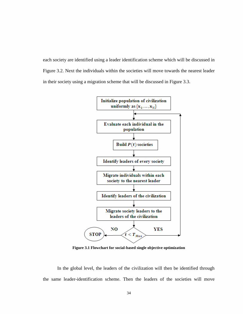
34

each society are identified using a leader identification scheme which will be discussed in

Figure 3.2. Next the individuals within the societies will move towards the nearest leader

in their society using a migration scheme that will be discussed in Figure 3.3.

Figure 3.1 Flowchart for social-based single objective optimization

In the global level, the leaders of the civilization will then be identified through

the same leader-identification scheme. Then the leaders of the societies will move

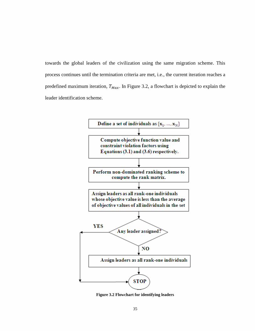
35

towards the global leaders of the civilization using the same migration scheme. This

process continues until the termination criteria are met, i.e., the current iteration reaches a

predefined maximum iteration, . In Figure 3.2, a flowchart is depicted to explain the

leader identification scheme.

Figure 3.2 Flowchart for identifying leaders

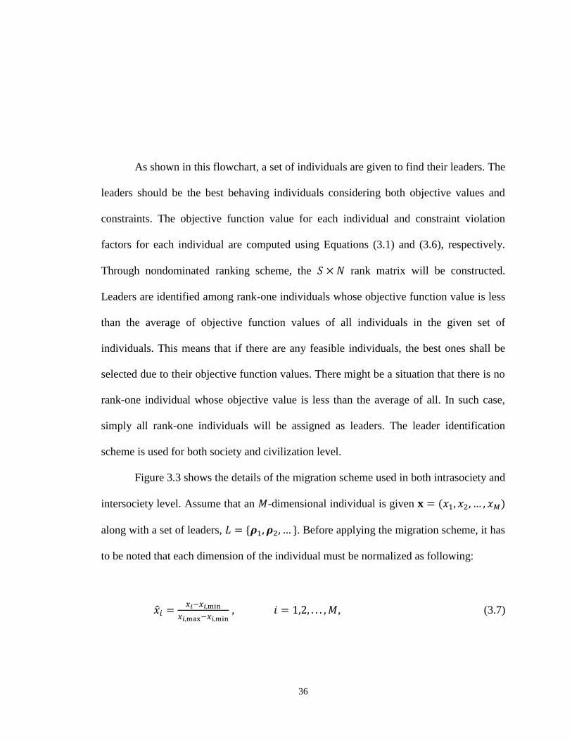
36

As shown in this flowchart, a set of individuals are given to find their leaders. The

leaders should be the best behaving individuals considering both objective values and

constraints. The objective function value for each individual and constraint violation

factors for each individual are computed using Equations (3.1) and (3.6), respectively.

Through nondominated ranking scheme, the rank matrix will be constructed.

Leaders are identified among rank-one individuals whose objective function value is less

than the average of objective function values of all individuals in the given set of

individuals. This means that if there are any feasible individuals, the best ones shall be

selected due to their objective function values. There might be a situation that there is no

rank-one individual whose objective value is less than the average of all. In such case,

simply all rank-one individuals will be assigned as leaders. The leader identification

scheme is used for both society and civilization level.

Figure 3.3 shows the details of the migration scheme used in both intrasociety and

intersociety level. Assume that an -dimensional individual is given

along with a set of leaders, . Before applying the migration scheme, it has

to be noted that each dimension of the individual must be normalized as following:

, , (3.7)

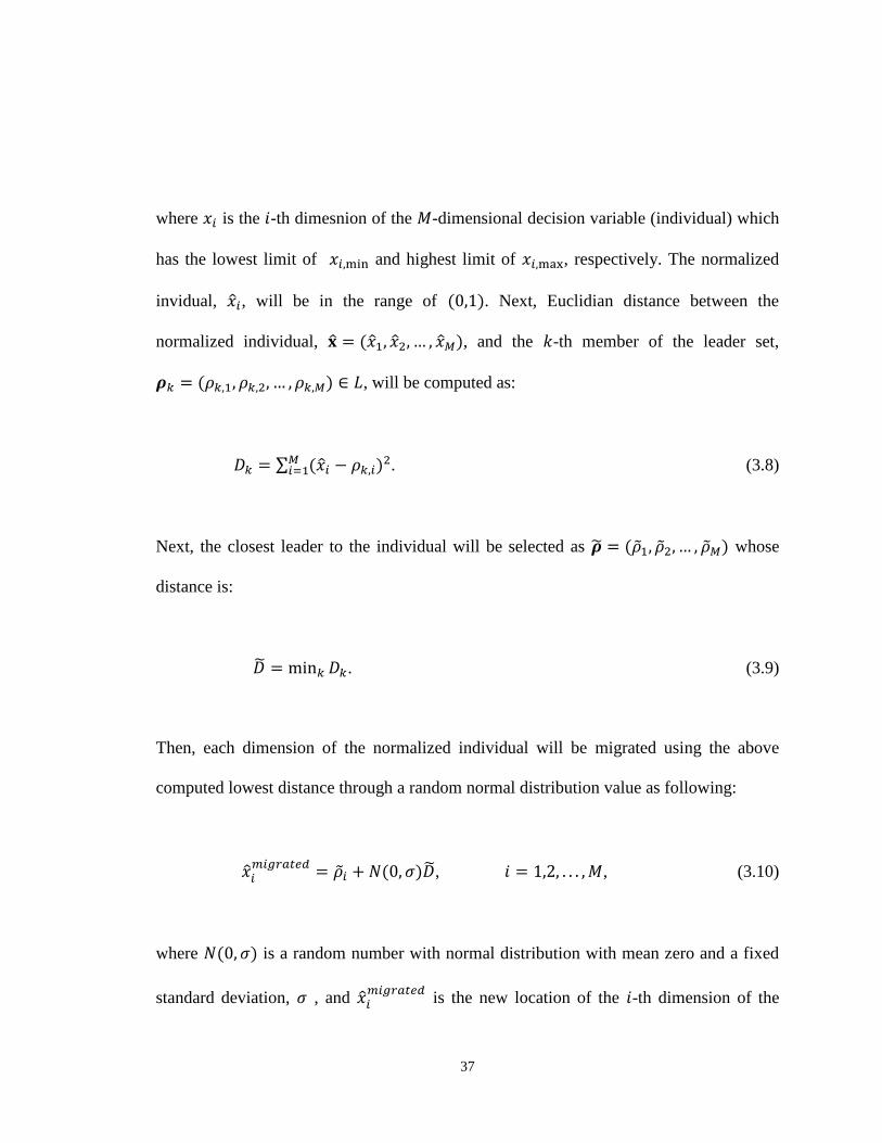
37

where is the -th dimesnion of the -dimensional decision variable (individual) which

has the lowest limit of and highest limit of , respectively. The normalized

invidual, , will be in the range of . Next, Euclidian distance between the

normalized individual, , and the -th member of the leader set,

, will be computed as:

. (3.8)

Next, the closest leader to the individual will be selected as whose

distance is:

. (3.9)

Then, each dimension of the normalized individual will be migrated using the above

computed lowest distance through a random normal distribution value as following:

, , (3.10)

where is a random number with normal distribution with mean zero and a fixed

standard deviation, , and

is the new location of the -th dimension of the

38

individual. As the final step, the migrated position should be rescaled back to the original

scale as following:

Figure 3.3 Flowchart on how to migrate individuals

, . (3.11)

It should be noted that migration scheme explained here is adopted in both

intrasociety level, migrating the individuals towards their society leaders, and intersociety

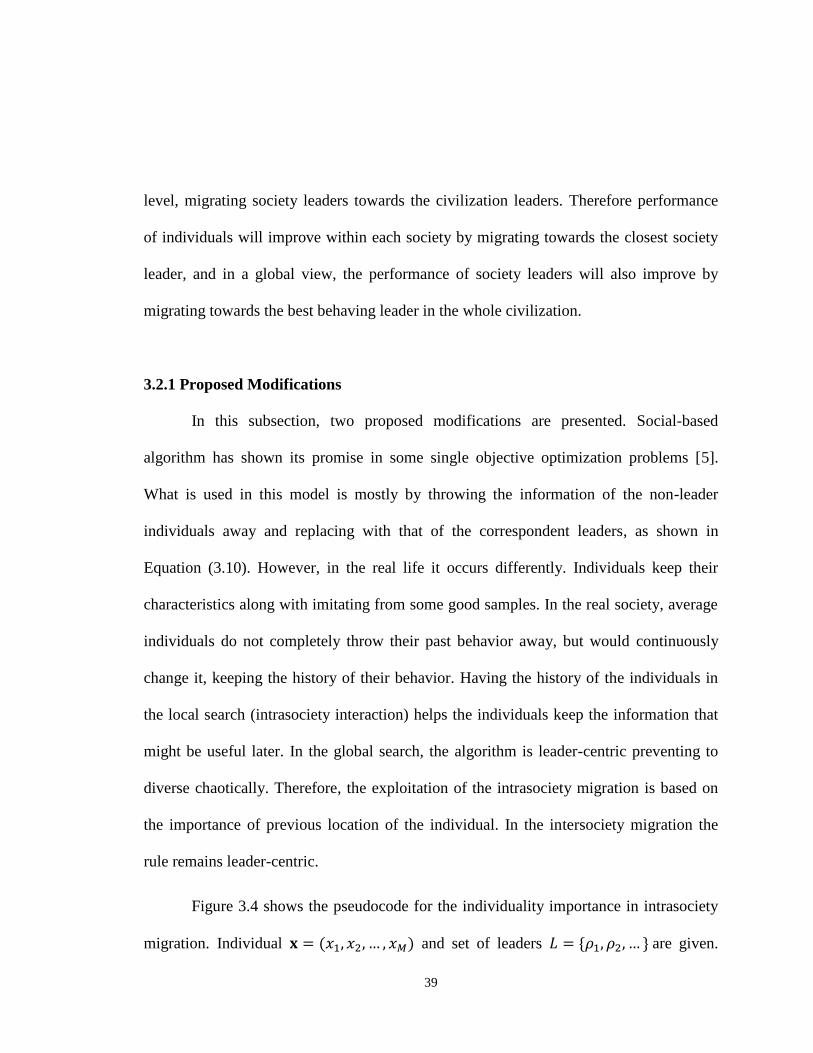
39

level, migrating society leaders towards the civilization leaders. Therefore performance

of individuals will improve within each society by migrating towards the closest society

leader, and in a global view, the performance of society leaders will also improve by

migrating towards the best behaving leader in the whole civilization.

3.2.1 Proposed Modifications

In this subsection, two proposed modifications are presented. Social-based

algorithm has shown its promise in some single objective optimization problems [5].

What is used in this model is mostly by throwing the information of the non-leader

individuals away and replacing with that of the correspondent leaders, as shown in

Equation (3.10). However, in the real life it occurs differently. Individuals keep their

characteristics along with imitating from some good samples. In the real society, average

individuals do not completely throw their past behavior away, but would continuously

change it, keeping the history of their behavior. Having the history of the individuals in

the local search (intrasociety interaction) helps the individuals keep the information that

might be useful later. In the global search, the algorithm is leader-centric preventing to

diverse chaotically. Therefore, the exploitation of the intrasociety migration is based on

the importance of previous location of the individual. In the intersociety migration the

rule remains leader-centric.

Figure 3.4 shows the pseudocode for the individuality importance in intrasociety

migration. Individual and set of leaders are given.

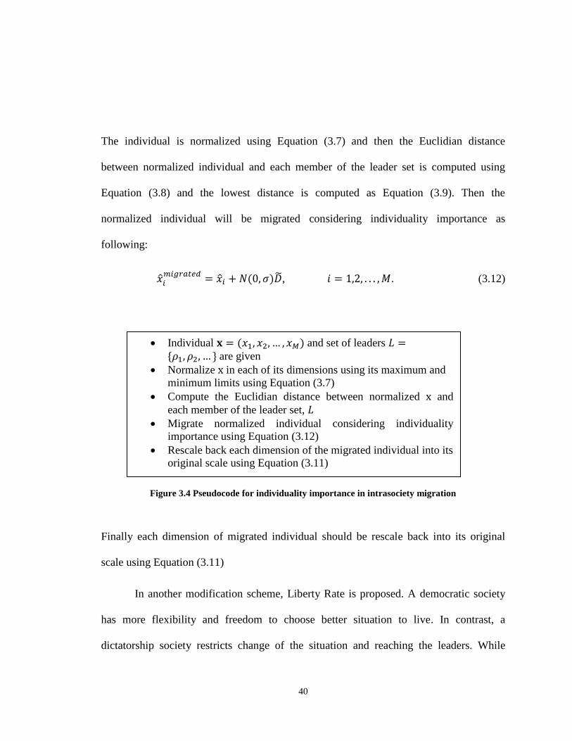
40

The individual is normalized using Equation (3.7) and then the Euclidian distance

between normalized individual and each member of the leader set is computed using

Equation (3.8) and the lowest distance is computed as Equation (3.9). Then the

normalized individual will be migrated considering individuality importance as

following:

, . (3.12)

Figure 3.4 Pseudocode for individuality importance in intrasociety migration

Finally each dimension of migrated individual should be rescale back into its original

scale using Equation (3.11)

In another modification scheme, Liberty Rate is proposed. A democratic society

has more flexibility and freedom to choose better situation to live. In contrast, a

dictatorship society restricts change of the situation and reaching the leaders. While

Individual and set of leaders are given

Normalize in each of its dimensions using its maximum and

minimum limits using Equation (3.7)

Compute the Euclidian distance between normalized and

each member of the leader set,

Migrate normalized individual considering individuality

importance using Equation (3.12)

Rescale back each dimension of the migrated individual into its

original scale using Equation (3.11)

41

individuals in a liberal society can migrate easily to be closer to the leaders, individual in

a less liberal society will experience difficulty to move near the leaders. So giving

preferences to approach to the leaders for different societies will improve the

convergence to the optimized solution. Different society will have different collective

behavior measure, called Liberty Rate. The higher liberty rate a society has, the more

flexible individuals in such society can move.

The Liberty Rate of a society is proposed as the relative ratio of average objective

functions of the society over the average objective functions of the civilization,

formulated as following:

, (3.13)

where is a predefined normalization constant and is the measure of the collective

behavior of the -th society, defined as the average of the objective values of the

individuals who belong to the -th society, formulated as:

, (3.14)

where is number of individuals in the -th society. , the measure for the civilization’s

collective behavior is also defined as:

. (3.15)

42

Then to migrate each individual in the -th society, a liberty-based migration is

performed as following:

, . (3.16)

3.3 Simulation Results

Spring Design is a mechanical design problem [116] to minimize the weight of a

tension/compression spring as shown in Figure 3.5. There are nonlinear inequality

constraints on minimum deflection, shear stress, surge frequency, limits on outside

diameter and on design variables. The design variables are the mean coil diameter, , the

wire diameter, , and the number of active coils, , along with four inequality

constraints. The mathematical formulation of the problem is as the following:

, (3.17)

(3.18)

,

,

,

,

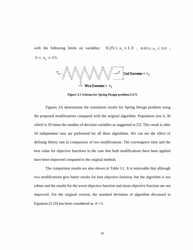
43

with the following limits on variables: 3.125.0 1 x , 0.205.0 2 x ,

152 3 x .

Figure 3.5 Schema for Spring Design problem [117]

Figures 3.6 demonstrate the simulation results for Spring Design problem using

the proposed modifications compared with the original algorithm. Population size is 30

which is 10 times the number of decision variables as suggested in [5]. This result is after

50 independent runs are performed for all three algorithms. We can see the effect of

defining liberty rate in comparison of two modifications. The convergence time and the

best value for objective functions in the case that both modifications have been applied

have been improved compared to the original method.

The comparison results are also shown in Table 3.1. It is noticeable that although

two modifications give better results for best objective function, but the algorithm is not

robust and the results for the worst objective function and mean objective function are not

improved. For the original version, the standard deviation of algorithm discussed in

Equation (3.10) has been considered as 1 .

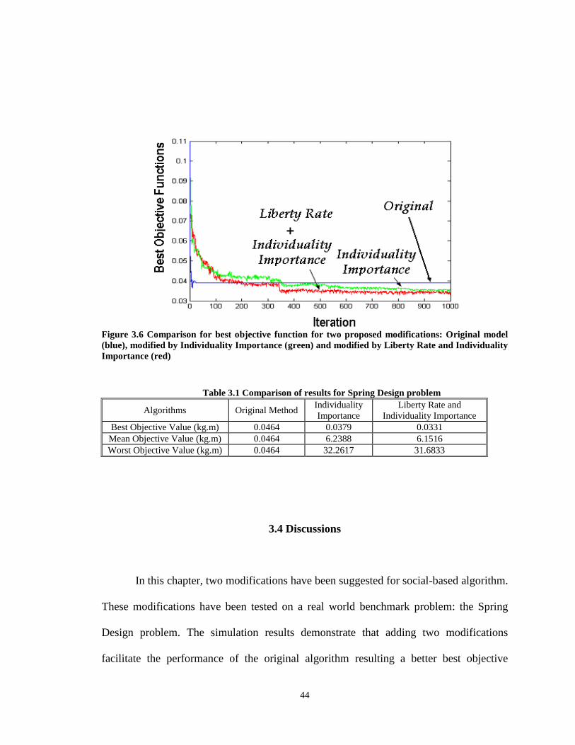
44

Figure 3.6 Comparison for best objective function for two proposed modifications: Original model

(blue), modified by Individuality Importance (green) and modified by Liberty Rate and Individuality

Importance (red)

Table 3.1 Comparison of results for Spring Design problem

Algorithms Original Method Individuality

Importance

Liberty Rate and

Individuality Importance

Best Objective Value (kg.m) 0.0464 0.0379 0.0331

Mean Objective Value (kg.m) 0.0464 6.2388 6.1516

Worst Objective Value (kg.m) 0.0464 32.2617 31.6833

3.4 Discussions

In this chapter, two modifications have been suggested for social-based algorithm.

These modifications have been tested on a real world benchmark problem: the Spring

Design problem. The simulation results demonstrate that adding two modifications

facilitate the performance of the original algorithm resulting a better best objective

45

values. The first modified algorithm, individuality-based social algorithm outperforms

the original social algorithm, while the liberty/individuality-based social algorithm

outperforms both the original social algorithm and the individuality-based social

algorithm in finding the best objective values. Both modified algorithms have migration

policy better than the original social algorithm. The original algorithm is basically biased

around the best performing individual which may result settling into a local optimum,

while both modified versions are based upon individual’s previous performance.

The results of modified version of social algorithm is based upon two hypotheses,

one is that information from all individuals must be collected and exploited to migrate to

the best leader, while the other is that the rate of convergence in different societies is not

necessarily the same and depends on the relative collective behavior of the individuals in

the society with respect to the civilization. Indeed the result in this case is improved

because of giving more weight to diversity to the search in the individual space. If we just

throw away all the non-leaders individuals, we lose a lot of information that might be

critical in the search process, however getting information from the other non-leaders

individuals might add to the convergence time.

The best objective values obtained in both modified versions are better than

original social algorithm; however the worst and mean values are not better than original

algorithm, since we are keeping the diversity while evolving. This also implies room for

further improvements in the future research.

46

CHAPTER IV

DIVERSITY-BASED INFORMATION EXCHANGE FOR PARTICLE SWARM

OPTIMIZATION

4.1 Introduction

Particle swarm optimization (PSO) is based on the changes of the positions and

velocities of the particles in a manner that optimizes a goal function. PSO has

demonstrated a promising performance for many problems; yet its fast convergence often

leads to premature convergence in local optima. The tradeoff between fast convergence

and being trapped in local optima will be even more critical in multimodal functions

having many local optima very close to each other. In order to escape from the local

optima and avoid premature convergence, the search for global optimum should be

diverse. Many researchers have improved the performance of the PSO by enhancing its

ability with a more diverse search. Specifically, some have proposed to use multiple

swarms each running independent PSO, and then exchange information among them.

Exchanging information among clusters has also been adopted as an important

design in several computational methods. Distributed genetic algorithm [6] employs GA

mechanism to evolve several subpopulations in parallel. During frequent migration

47

among subpopulations, some individuals from each subpopulation will be sent to another

subpopulation to replace other individuals based upon a replacement policy. In another

algorithm known as society and civilization model [5], individuals from multiple

societies would cooperate with each other in order to enhance their performance. The

migration in this model occurs in two levels; first, the migrating of individuals inside

each society toward the society leaders (intrasociety level), and second, the migrating of

society leaders toward the civilization leaders (intersociety level).

In this study, a method borrowed from distributed genetic algorithm is employed

to exchange information among multiple swarms in PSO. At regular intervals, each

swarm prepares two sets of particles. One set is the particles that must be sent to another

swarm and another set is the particles that must be replaced by individuals from other

swarms. To prepare these two sets of particles, diversity measure is considered as the

primary goal instead of only performance of the particles. When particles are

approaching the local optima, several of them will have similar positional information.

This similar redundant information will be replaced by particles from other swarms. This

algorithm also proposes a new paradigm to find each swarm’s neighbors. The

neighborhood between swarms is defined by the use of Hamming distance between

representatives of each pair of swarms. The particle’s movement in the space is based on

one variation of PSO with three basic terms, each one leading the particles toward the

best particles in its own swarm, in its swarm’s neighborhood, and in the whole

population.

48

The structure of this chapter is organized as follows. Section 4.2 reviews the

related studies in this field. In Section 4.3, the proposed algorithm is explained in detail.

The main ideas of the proposed method are shown. In Section 4.4, the simulation of the

proposed algorithm is performed on a set of hard benchmark problems. Section 4.5

summarizes the benefits of the proposed paradigm on PSO and outlines the future work

for multiobjective optimization problems due to the nature of the diversity promotion

proposed.

4.2 Review of Related Work

Kennedy and Eberhart [1] introduced the particle swarm optimization, an

algorithm based on imitating behavior of flocking birds. It mimics grouping of birds as

particles, their random movement, and regrouping them again to generate a model so that

it can solve engineering optimization problems. Particles are known with their positions

and velocities and can be updated using:

, (4.1)

,


position ever experienced of each particle, and is the best position ever attained

49

among all particles. and are random numbers uniformly generated in the range of

. , , and are personal, social, and momentum coefficients that are predefined.

The main problem for PSO is its fast convergence to local optima. Later, Kennedy [46]

introduced the stereotyping of the particles in which substitution of cluster centers for

showed appreciable improvement of the PSO performance. His research suggested

that PSO is more effective when individuals are attracted toward the center of their own

clusters.

In multimodal problems, the search effort needs to be diverse in order to find the

global optimum among a set of many local optima. The fast converging behavior of the

PSO makes this issue so critical for multimodal problems. To achieve a more diverse

search, Al-Kazemi and Mohan [47] divided the population into two sets at any given

time, one set moving to the while another moving in opposite direction by

selecting appropriate fixed values for in each set. After some iterations, if the

is not improved, then the particles would switch their group. Baskar and

Suganthan [48] in their concurrent PSO used two swarms to search concurrently for a

solution along with frequent passing of information, which was the of two

cooperating swarms. After each exchange, the two swarms had to track the better

found. One of the swarms was using regular PSO, and the other was using the Fitness-to-

Distance ratio PSO [49]. Their approach improved the performance over both methods in

solving single objective optimization problems. El-Abd and Kamel [50] further improved

the previous algorithm by adding a two-way flow of information between two swarms. In

50

their algorithm, when exchanging the best particle between two swarms, this particle is

used to replace the worst particle in another swarm. The two swarms perform a fixed

number of iterations, and then the best particles inside each swarm will replace the

worst particles in the other swarm only if they have a better fitness. This makes it

possible for both swarms to exchange new information from the other swarm’s

experience. Krohling et al. [51] proposed co-evolutionary PSO in which two populations

of PSO are involved. One PSO runs for a specified number of iterations while the other

remains static and serves as its environment. At the end of such period, values

obtained in previous cycles have to be re-evaluated according to the new environment

before starting evolution. Although these algorithms used information exchange among

swarms, but none of them adopted specific paradigm based on promoting diversity in

selecting and sending particles from one swarm to another.

On the other hand, one of the main concerns in multiobjective optimization

problems (MOP) is also to search for a diverse set of potential solutions, known as Pareto

front. There have been several algorithms to extend PSO to handle diversity issue in

MOPs. Parspopoulos et al. [52] introduced vector evaluated particle swarm optimizer

(VEPSO) to solve multiobjective problems. A VEPSO is a multi-swarm variant of PSO

in which each swarm is evaluated using only one of the objective functions of the

problem under consideration, and the information it possesses for this objective function

is communicated to the other swarms through the exchange of their best experience. In

VEPSO, the velocity of the particles in each swarm is updated using the best previous

51

position, , of another selected swarm. Selection of this swarm in the migration

scheme can be either random or in a sequential order. Ray and Liew [53] used Pareto

dominance and combined concepts of evolutionary techniques with the particle swarm.

This algorithm uses crowding distance to preserve diversity. Hu and Eberhart [54] in their

dynamic neighborhood PSO proposed an algorithm to optimize only one objective at a

time. The algorithm may be sensitive to the optimizing order of objective functions.

Fieldsend and Singh [55] proposed an approach in which they used an unconstrained elite

archive to store the nondominated individuals found along the search process. The

archive interacts with the primary population in order to define local guides. Mostaghim

and Teich [56, 60] introduced a sigma method in which the best local guides for each

particle are adopted to improve the convergence and diversity of the PSO. Li [57]

adopted the main idea from NSGA-II into the PSO algorithm. Coello Coello et al. [58],

on the other hand, proposed an algorithm using a repository for the nondominated

particles along with adaptive grid to select the global best of PSO. The algorithms

proposed to solve MOPs using PSO are based upon promoting the nondominated

particles at any given time, not exploiting the information of all particles in the

population.

The information exchange through migration in order to increase the search

ability of the algorithm has been used in some other innovated paradigms. Ray and Liew

[5] introduced their society and civilization model for optimization in accordance with

simulation of social behavior. Individuals in a society interact with each other in order to

52

improve. Such improvement is done by information acquisition from the better-

performing individuals or leaders in that society. This intrasociety interaction will

improve the individual’s performance, but cannot improve the leader’s performance. The

leaders do communicate externally with the leaders of other societies to improve. This

intersociety communication leads to migration of the leaders to developed societies,

which in turn, moves the overall poor-performing societies toward better-performing

ones. At first, population is clustered into several mutually exclusive ones based on their

distance in parametric space. Then objective functions along with constraints (if any) lay

down a ranking system to choose the leaders in each cluster, and then migration in two

levels will take place. Society and civilization model showed competitive results on

single objective constrained optimization problems with respect to GAs.

The concept of having multiple sets had been originally introduced and used in

distributed genetic algorithm (DGA) [6]. In DGA, population is divided into several

subpopulations each running its own GA independently. At regular time intervals, inter-

processor communication will happen. During this migration stage, a proportion of each

subpopulation is selected and sent to another subpopulation. The migrant individuals will

replace others based on replacement policy. In another kind of distributed evolutionary

algorithm, Ursem [4] adopted his multinational evolutionary algorithm using a spatially

separated model. He applied a fitness-topology function, instead of clustering, to decide

on the relationship between a point and a cluster. The algorithm was to find all peaks of a

multimodal function in unconstrained optimization problems.

53

In DGA, there are different policies on selection of migrants and replacement of

individuals within each of the subpopulations. Cantu-Paz [118] showed that sending the

fittest individuals of the population and replacing individuals with low fitness produces

the best results. Denzinger and Kidney [18] used a diversity measure to select individuals

for migration. Power et al. [119] used a method for selection based on a diverse set of

individuals rather than the highly fit ones. The reason is to avoid like information to be

sent to another subpopulation. Sometimes the majority of individuals can be located very

close to each other, especially in the last steps of convergence. Therefore, by selecting the

fittest individuals, the similar individuals from a small area will be sent to the next

subpopulation. In case the algorithm is likely to be trapped in a local optima, this similar

information is useless to diversify the search and get away from the local optima. Instead,

the basis is to choose a diversified list of individuals to send to the other GAs. The

sending list will be filled by the following individuals in this order: (1) an average

individual of the subpopulation as representative of the population, (2) m individuals

based on closeness to this representative whose fitness is better than representative, (3) m

individuals based on closeness to this representative whose fitness is poorer than

representative, and finally (4) the fittest individual in the subpopulation. There will also

be a replacement list that will be filled in the following order: (1) individuals having

similar genetic information, by order of fitness, with least fit ones being replaced before

better fit ones, and (2) individuals with lowest fitness values. Their method was applied

to single objective multimodal optimization and showed significantly better results when

54

compared to standard DGA with send-best-replace-worst strategy.

4.3 Diversity-based Information Exchange among Swarms in PSO

The underline principle of the proposed algorithm is based upon the idea of

exploiting the information of all particles in the population. The population will be

divided into P swarms, and each swarm will perform a PSO paradigm. After some

predefined iterations, the swarms will exchange information based on a diversified list of

particles. Each swarm prepares a list of sending particles to be sent to the next swarm,

and also prepares a list of replacement particles to be replaced by particles coming from

other swarms. Each swarm chooses the leaders of the next generation from the updated

swarm after exchange of particles. To select the list of particles to send, algorithm uses a

strategy according to the locations of the particles in the swarm and their objective values

instead of their objective values alone. A list is prepared in the following order.

Priority S1: The higher priority in the selection of particles is given to a particle

that has the least average Hamming distance from others. This particle is considered as

the representative of the swarm. The average Hamming distance between each pair of

particles in the swarm is calculated and then the least among them is found.

Priority S2: The closest particles to the representative particle whose objective

value is greater than that of the representative will be chosen. is a value that depends

on the rate of information exchange, , (a predefined value between 0 and 1) among

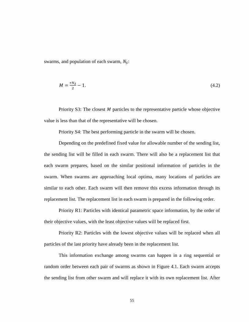
55

swarms, and population of each swarm, :

. (4.2)

Priority S3: The closest particles to the representative particle whose objective

value is less than that of the representative will be chosen.

Priority S4: The best performing particle in the swarm will be chosen.

Depending on the predefined fixed value for allowable number of the sending list,

the sending list will be filled in each swarm. There will also be a replacement list that

each swarm prepares, based on the similar positional information of particles in the

swarm. When swarms are approaching local optima, many locations of particles are

similar to each other. Each swarm will then remove this excess information through its

replacement list. The replacement list in each swarm is prepared in the following order.

Priority R1: Particles with identical parametric space information, by the order of

their objective values, with the least objective values will be replaced first.

Priority R2: Particles with the lowest objective values will be replaced when all

particles of the last priority have already been in the replacement list.

This information exchange among swarms can happen in a ring sequential or

random order between each pair of swarms as shown in Figure 4.1. Each swarm accepts

the sending list from other swarm and will replace it with its own replacement list. After

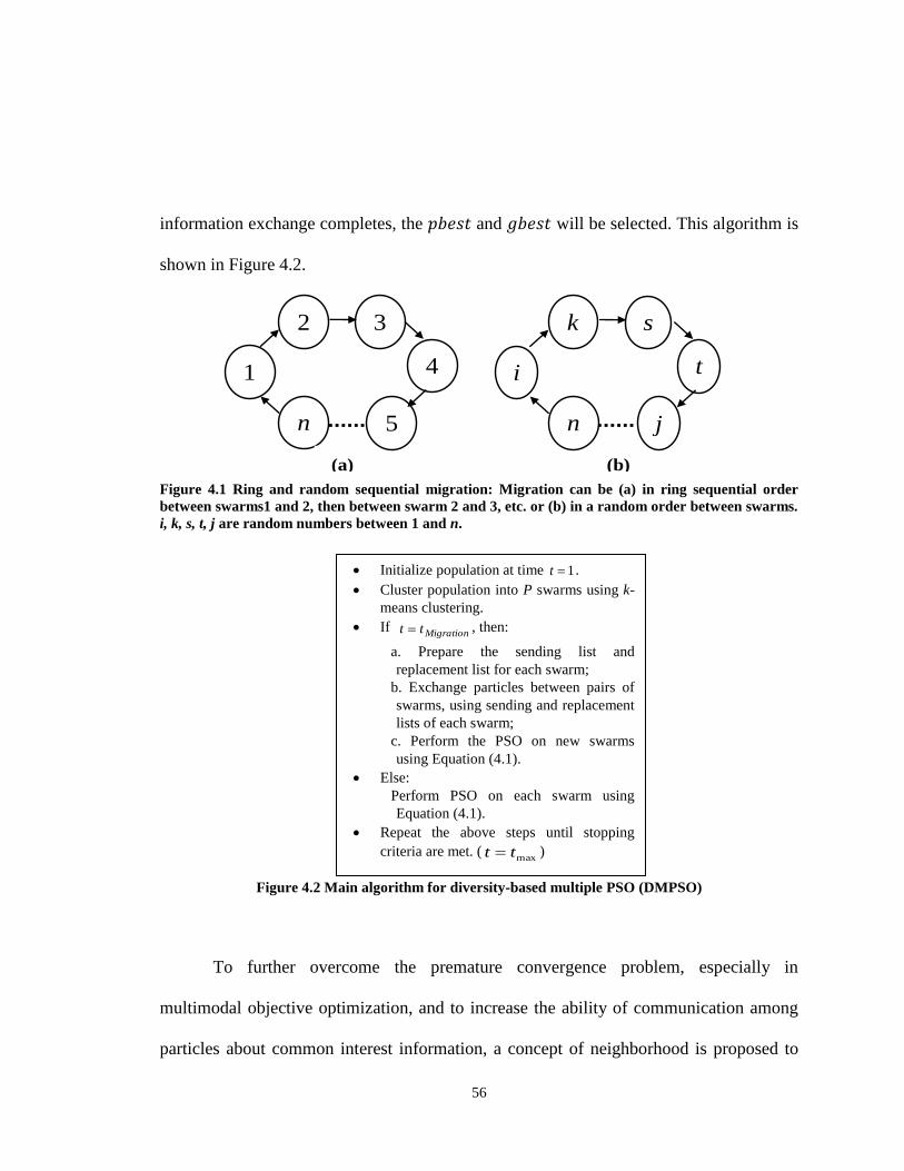
56

information exchange completes, the and will be selected. This algorithm is

shown in Figure 4.2.

Figure 4.1 Ring and random sequential migration: Migration can be (a) in ring sequential order

between swarms1 and 2, then between swarm 2 and 3, etc. or (b) in a random order between swarms.

i, k, s, t, j are random numbers between 1 and n.

Figure 4.2 Main algorithm for diversity-based multiple PSO (DMPSO)

To further overcome the premature convergence problem, especially in

multimodal objective optimization, and to increase the ability of communication among

particles about common interest information, a concept of neighborhood is proposed to

1

2 3

4

5 n

i

k s

t

j n

(a) (b)

Initialize population at time 1t .

Cluster population into P swarms using k-

means clustering.

If Migrationtt , then:

a. Prepare the sending list and

replacement list for each swarm;

b. Exchange particles between pairs of

swarms, using sending and replacement

lists of each swarm;

c. Perform the PSO on new swarms

using Equation (4.1).

Else:

Perform PSO on each swarm using

Equation (4.1).

Repeat the above steps until stopping

criteria are met. (maxtt )

57

promote the particles in a neighborhood to utilize and share information among

themselves. For the PSO schema, a three-level mechanism is adopted. In personal level,

particle in a swarm will follow the leader of the swarm that is the best behaving particle

in that swarm. In neighborhood level, the particle will simultaneously follow the best

behaving particle in its neighborhood to achieve a synchronized behavior in the

neighborhood and to share the information, and finally in the global level, particles of

each swarm will follow the best behaving particle in the whole population, seeking a

global goal. This paradigm of PSO is formulated as:

, (4.3)

,


position in the cluster, is the best position among all particles and is the best

position among the particles’ neighborhood. , , and are random numbers uniformly

generated in the range of . Thus particles always move statistically towards the

direction of , , and in order to use the past experience in the search

process. , , and are constant values representing the weight of each of the terms

of personal, global, and neighborhood behavior and is the momentum for previous

velocity. It should be noted that the unified PSO [120] integrates the local best and global

best PSOs into a single equation to update the velocity of particles based on the global

58

best particle, the neighboring best particle, and the particle’s own best position, while in

the proposed paradigm, velocity updates using the best particle in the cluster of particles,

the best particle in the neighboring swarms, and the best global particle with no

restriction on the weights.

To find the neighborhood among particles in PSO, there have been different

strategies used by researchers [37, 121]. Some have applied ring neighborhood, the von

Neumann neighborhood, or some other topological neighborhoods. The proposed

definition of neighborhood is to define neighboring swarms according to the average as

representative of each swarm to decide whether the swarms are in neighborhood of each

other. In the i-th swarm with the particles of , the representative, , is

defined by centroid of all particles:

(4.4)

The inter-swarm distance between swarms i and j, , is defined by the inner

products of two vectors:

, (4.5)

where is the k-th element of the representative .

59

Swarms are defined to be in a neighborhood if and only if all inter-swarm

distances among them are less than the average inter-swarm distance: , ,

… and , where

, where P is the number of swarms.

Figure 4.3 Schema of swarm neighborhood: Swarms 1, 2 and 3 are in a neighborhood, since ,

and but swarm 4 does not belong to this neighborhood. Notice that even

but . Swarms 4, 5 and 6 form another neighborhood, because , and . Swarm 3 does not belong to this neighborhood because even but . (Solid circles

denote the representative points of each swarm)

For example, for two of them, swarms i and j are in a neighborhood if and only if

. If but , then swarm k does not belong to this neighborhood. In

Figure 4.3, an example with six swarms is shown. Swarms 1, 2 and 3 are in a

neighborhood because , and but swarm 4 does not belong to

R13

Swarm 3

Swarm 2

R23 R12

R45

R56

R46

Swarm 4

Swarm 5

Swarm 6

R14

R34

Swarm 1

Size of R

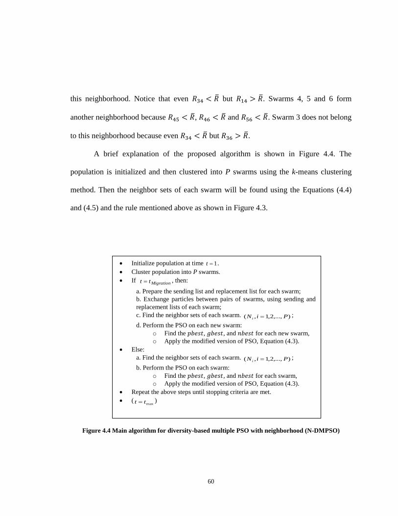
60

this neighborhood. Notice that even but . Swarms 4, 5 and 6 form

another neighborhood because , and . Swarm 3 does not belong

to this neighborhood because even but .

A brief explanation of the proposed algorithm is shown in Figure 4.4. The

population is initialized and then clustered into P swarms using the k-means clustering

method. Then the neighbor sets of each swarm will be found using the Equations (4.4)

and (4.5) and the rule mentioned above as shown in Figure 4.3.

Figure 4.4 Main algorithm for diversity-based multiple PSO with neighborhood (N-DMPSO)

Initialize population at time 1t .

Cluster population into P swarms.

If Migrationtt , then:

a. Prepare the sending list and replacement list for each swarm;

b. Exchange particles between pairs of swarms, using sending and

replacement lists of each swarm;

c. Find the neighbor sets of each swarm. ),...,2,1,( PiN i ;

d. Perform the PSO on each new swarm:

o Find the , , and for each new swarm,

o Apply the modified version of PSO, Equation (4.3).

Else:

a. Find the neighbor sets of each swarm. ),...,2,1,( PiN i ;

b. Perform the PSO on each swarm:

o Find the , , and for each swarm,

o Apply the modified version of PSO, Equation (4.3).

Repeat the above steps until stopping criteria are met.

(maxtt )

61

To perform the PSO according to Equation (4.3), we have to find the best

performing particle in each swarm, namely the , the best performing particle in the

all-neighbor sets of that swarm, namely the and the best performing particle in the

whole population, . This process will be iterated until the time for migration is

reached. At regular fixed intervals, each swarm prepares a list of particles to send to the

next swarm, a list of particles that must be replaced from other particles coming from

other swarms; then exchange of particles between each of the two swarms will happen

according to Figure 4.1. This algorithm including clustering, information exchange, and

flight of particles will continue until the stopping criteria are met.

4.4 Simulation Results

The proposed algorithm was tested using some benchmark problems, which are

often used to examine GA solving multimodal problems [4, 122]. These problems

adopted from [119] vary in difficulty and dimension. In order to test the proposed

algorithm, its performance has been compared with two distributed genetic algorithms

[118-119]. One of them is DGA with a standard migration policy (SDGA), best-sent-

worst-replaced [118]. The other one is a DGA with diversity-based migration policy

(DDGA) [119]. In order to draw a fair comparison, the same rate of information

exchange as their migration rate has been adopted. The main population for the proposed

algorithms DMPSO and N-DMPSO was set as 50 particles. The k-means clustering

62

method was used with m=6 swarms. The coefficients of , , , and are selected as

1.4, 1.4, 1.4, and 0.8, respectively. The rate of information exchange is varied with the

values of 0.05, 0.2, and 0.4. At the time interval of , particles are exchanged

among swarms.

The first problem used to test the proposed algorithm is F1 [119] with five peaks

and four valleys between each of the two neighboring peaks. This function is depicted in

Figure 4.5. Figure 4.5(a) shows a 3-D landscape while Figure 4.5(b) displays the contour

map of the function F1. The results of applying both proposed algorithms are shown in

Table 4.1. The optimal solution found (in percentage) is calculated out of 30 independent

runs for each algorithm. The solution is considered to be optimal when the optimal

objective value of 2.5 is reached. The best objective values for the final solution is

averaged over 30 runs to obtain the mean best objective reported in the table. Each

algorithm is performed for three values of rate of information exchange, 0.05, 0.2, and

0.4. The best performing algorithm in each case is shown in bold face. The graphical

view of the location of the best particles of the final solution is depicted in Figure 4.6.

Figure 4.6 (a) and (b) are for DMPSO with rate of information exchange equal to

0.05 and 0.4, and (c) and (d) are for N-DMPSO with rate of information exchange equal

to 0.05 and 0.4, respectively. Figure 4.6 shows that some of the particles in DMPSO will

be trapped in local maxima (0.897,0) and (-0.897,0). In N-DMPSO, most particles

approached toward (0,0), the global maximum. The results in Table 4.1 show that both

proposed algorithms perform better and N-DMPSO outperforms all of them.

63

The second benchmark problem is F2 [119] with 10 peaks shown in Figure 4.7.

The results of the algorithms are also shown in Table 4.1. The graphical view of the best

particles for both algorithms is obtained in Figure 4.8. This figure shows that some

particles in DMPSO are trapped in a local maximum while in N-DMPSO most particles

reach the global maximum. Results reported in Table 4.1 also show the better

performance of N-DMPSO.

The next benchmark function is F3 [119], shown in Figure 4.9, with two close

peaks and a valley between them. The results of the algorithms are summarized in Table

4.1 as well, and the graphical view of the best particles is depicted in Figure 4.10. Figure

4.10 shows that in DMPSO some of the particles are trapped in local maximum at (-

1.444,0), while in N-DMPSO most of the particles reached the global maximum at

(1.697,0). Table 4.1 also illustrates that N-DMPSO is outperforming other algorithms.

The next benchmark function is F4 [119] with a total of five peaks, one global maximum

and four local maxima in its neighborhood, shown in Figure 4.11. The results and the

graphical presentation of the best particles in Table 4.1 and Figure 4.12 show once again

that N-DMPSO has less particles trapped in four local maxima located at the corners of

the variable space. The results obtained in Table 4.1 confirm a higher number of found

optimal solutions. The benchmark function F5 [119] has six peaks, two of which are

global maxima as shown in Figure 4.13. The results of the algorithms are shown in

Figure 4.14 and Table 4.1. The D-DGA in this problem outperforms the proposed

algorithms when rate of information exchange is 0.05 and 0.2. On the other hand, with a

64

higher rate, the proposed algorithm performs better, i.e., when more particles are

exchanged, PSO shows more superiority.

The benchmark function of F6 [119] has a variable dimension. Three different

dimensions of 25, 40 and 50 have been used here. The rate of the information exchange

for this case and the remaining benchmark functions has been fixed at 0.1. The best

objective value for the final solutions is averaged over 30 runs and shown in Table 4.2.

The N-DMPSO outperforms the other three algorithms at dimensions 25 and 40 but at

dimension 50, D-DGA performs better. The benchmark function of F7 [119] has also a

variable dimension, and three dimensions of 25, 40, and 50 have been adopted here.

Results in Table 4.2 show that N-DMPSO outperforms the others at dimensions 25 and

40 but again, at dimension 50, D-DGA outperforms others. The next benchmark function,

F8 [119], has 10 variables. N-DMPSO also outperforms other algorithms in this case. And

finally, the last benchmark function F9 [119] has 40 variables. N-DMPSO performs better

than other algorithms as well. In general, N-DMPSO outperformed other algorithms in

several benchmark functions. It was outperformed in some cases, especially problems

with very high dimension, by D-DGA. It might be due to the nature of GA that

recombination demonstrates a better performance in high dimension; however it needs to

be tested more.

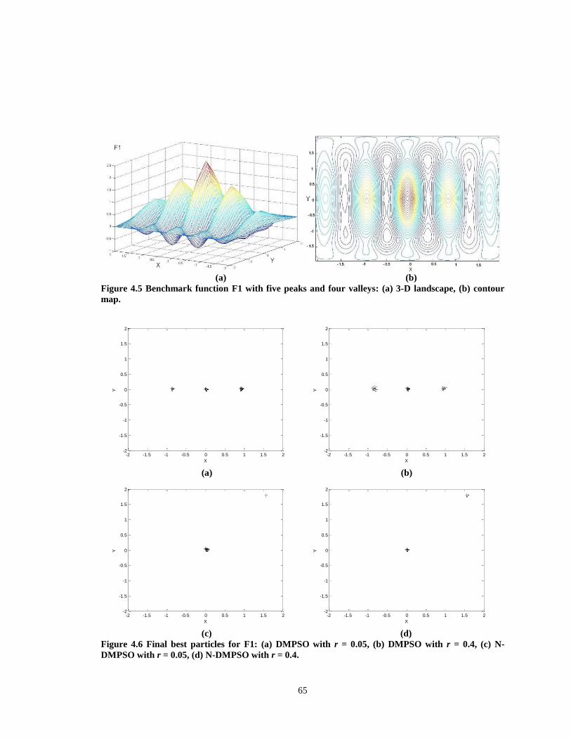
65

(a) (b)

Figure 4.5 Benchmark function F1 with five peaks and four valleys: (a) 3-D landscape, (b) contour

map.

(a) (b)

(c) (d)

Figure 4.6 Final best particles for F1: (a) DMPSO with r = 0.05, (b) DMPSO with r = 0.4, (c) N-

DMPSO with r = 0.05, (d) N-DMPSO with r = 0.4.

-2 -1.5 -1 -0.5 0 0.5 1 1.5 2-2

-1.5

-1

-0.5

0

0.5

1

1.5

2

X

Y

-2 -1.5 -1 -0.5 0 0.5 1 1.5 2-2

-1.5

-1

-0.5

0

0.5

1

1.5

2

X

Y

-2 -1.5 -1 -0.5 0 0.5 1 1.5 2-2

-1.5

-1

-0.5

0

0.5

1

1.5

2

X

Y

-2 -1.5 -1 -0.5 0 0.5 1 1.5 2-2

-1.5

-1

-0.5

0

0.5

1

1.5

2

X

Y

66

(a) (b)

Figure 4.7 Benchmark function F2 with 10 peaks: (a) 3-D landscape, (b) contour map.

(a) (b)

(c) (d)



-0.8 -0.6 -0.4 -0.2 0 0.2 0.4 0.6 0.8 1 1.2

-1

-0.5

0

0.5

1

X

Y

-0.8 -0.6 -0.4 -0.2 0 0.2 0.4 0.6 0.8 1 1.2

-1

-0.5

0

0.5

1

X

Y

-0.8 -0.6 -0.4 -0.2 0 0.2 0.4 0.6 0.8 1 1.2

-1

-0.5

0

0.5

1

X

Y

-0.8 -0.6 -0.4 -0.2 0 0.2 0.4 0.6 0.8 1 1.2

-1

-0.5

0

0.5

1

X

Y

67

(a) (b)

Figure 4.9 Benchmark function F3 with two peaks and one valley: (a) 3-D landscape, (b) contour

map.

(a) (b)

(c) (d)



-2.5 -2 -1.5 -1 -0.5 0 0.5 1 1.5 2 2.5

-2.5

-2

-1.5

-1

-0.5

0

0.5

1

1.5

2

2.5

X

Y

-2.5 -2 -1.5 -1 -0.5 0 0.5 1 1.5 2 2.5

-2.5

-2

-1.5

-1

-0.5

0

0.5

1

1.5

2

2.5

X

Y

-2.5 -2 -1.5 -1 -0.5 0 0.5 1 1.5 2 2.5

-2.5

-2

-1.5

-1

-0.5

0

0.5

1

1.5

2

2.5

X

Y

-2.5 -2 -1.5 -1 -0.5 0 0.5 1 1.5 2 2.5

-2.5

-2

-1.5

-1

-0.5

0

0.5

1

1.5

2

2.5

X

Y

68

(a) (b)

Figure 4.11 Benchmark function F4 with five peaks: (a) 3-D landscape, (b) contour map.

(a) (b)

(c) (d)



-2 -1.5 -1 -0.5 0 0.5 1 1.5 2

-2

-1.5

-1

-0.5

0

0.5

1

1.5

2

X

Y

-2 -1.5 -1 -0.5 0 0.5 1 1.5 2

-2

-1.5

-1

-0.5

0

0.5

1

1.5

2

X

Y

-2 -1.5 -1 -0.5 0 0.5 1 1.5 2

-2

-1.5

-1

-0.5

0

0.5

1

1.5

2

X

Y

-2 -1.5 -1 -0.5 0 0.5 1 1.5 2

-2

-1.5

-1

-0.5

0

0.5

1

1.5

2

X

Y

69

(a) (b)

Figure 4.13 Benchmark function F5 with six peaks, two of which are global maxima: (a) 3-D

landscape, (b) contour map.

(a) (b)

(c) (d)



-1.5 -1 -0.5 0 0.5 1 1.5

-1

-0.8

-0.6

-0.4

-0.2

0

0.2

0.4

0.6

0.8

1

X

Y

-1.5 -1 -0.5 0 0.5 1 1.5

-1

-0.8

-0.6

-0.4

-0.2

0

0.2

0.4

0.6

0.8

1

X

Y

-1.5 -1 -0.5 0 0.5 1 1.5

-1

-0.8

-0.6

-0.4

-0.2

0

0.2

0.4

0.6

0.8

1

X

Y

-1.5 -1 -0.5 0 0.5 1 1.5

-1

-0.8

-0.6

-0.4

-0.2

0

0.2

0.4

0.6

0.8

1

X

Y

70

Table 4.1 Results for optimal found (%) and mean best objective for F1, F2, F3 and F5

Algorithms S-DGA D-DGA DMPSO N-DMPSO

Max F1

Optimal

Found (%)

r = 0.05 0% 0.8% 10.0% 13.3%

r = 0.2 0% 13.3% 13.3% 20.0%

r = 0.4 0% 15.8% 16.7% 23.3%

Mean best

objective

r = 0.05 1.98898 2.48217 2.4801 2.4863

r = 0.2 1.97855 2.4605 2.4745 2.4793

r = 0.4 2.02455 2.48811 2.4891 2.4905

Max F2

Optimal

Found (%)

r = 0.05 0% 22.5% 33.3% 53.3%

r = 0.2 0.8% 5.8% 13.3% 26.6%

r = 0.4 0% 17.5% 23.3% 33.3%

Mean best

objective

r = 0.05 6.73371 8.58322 8.6739 8.6783

r = 0.2 6.70137 8.63548 8.6532 8.6621

r = 0.4 7.31735 8.68075 8.6923 8.6953

Max F3

Optimal

Found (%)

r = 0.05 0% 3.3% 16.7% 20.0%

r = 0.2 0% 20% 23.3% 33.3%

r = 0.4 0% 23.3% 43.3% 53.3%

Mean best

objective

r = 0.05 4.67853 4.812 4.8121 4.8127

r = 0.2 4.7159 4.810 4.8117 4.8136

r = 0.4 4.73849 4.81496 4.8151 4.8155

Max F4

Optimal

Found (%)

r = 0.05 3.3% 4.2% 16.7% 26.6%

r = 0.2 0% 42.5% 43.3% 53.3%

r = 0.4 0% 35% 36.7% 43.3%

Mean best

objective

r = 0.05 1.34999 1.48242 1.49016 1.49127

r = 0.2 1.33163 1.49341 1.49281 1.49332

r = 0.4 1.29936 1.49123 1.49178 1.49341

Max F5

Optimal

Found (%)

r = 0.05 11.7% 67.5% 43.3% 53.3%

r = 0.2 14.2% 69.2% 33.3% 36.7%

r = 0.4 0.8% 22.5% 36.6% 43.3%

Mean best

objective

r = 0.05 0.970634 1.03 1.0283 1.0297

r = 0.2 0.975198 1.03006 1.0281 1.0288

r = 0.4 0.941727 1.02874 1.0293 1.0297

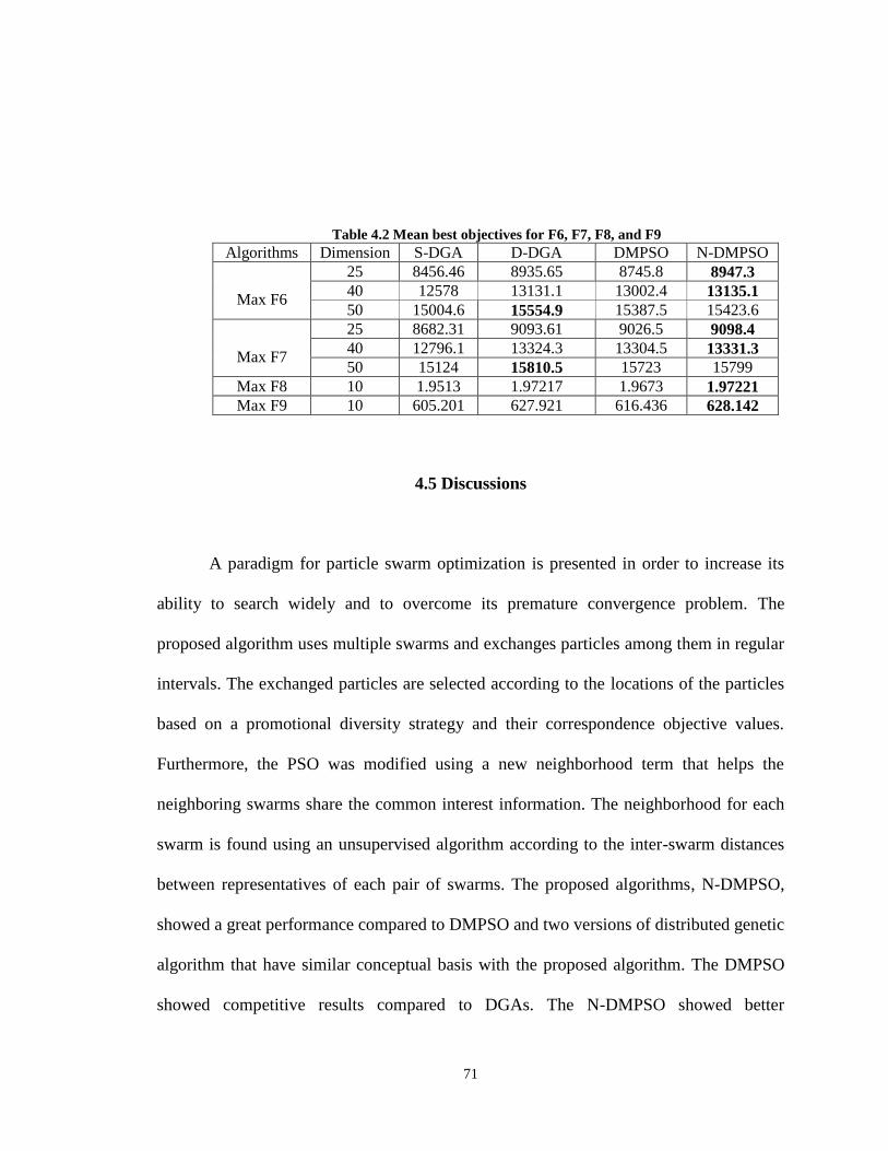
71

Table 4.2 Mean best objectives for F6, F7, F8, and F9

Algorithms Dimension S-DGA D-DGA DMPSO N-DMPSO

Max F6

25 8456.46 8935.65 8745.8 8947.3

40 12578 13131.1 13002.4 13135.1

50 15004.6 15554.9 15387.5 15423.6

Max F7

25 8682.31 9093.61 9026.5 9098.4

40 12796.1 13324.3 13304.5 13331.3

50 15124 15810.5 15723 15799

Max F8 10 1.9513 1.97217 1.9673 1.97221

Max F9 10 605.201 627.921 616.436 628.142

4.5 Discussions

A paradigm for particle swarm optimization is presented in order to increase its

ability to search widely and to overcome its premature convergence problem. The

proposed algorithm uses multiple swarms and exchanges particles among them in regular

intervals. The exchanged particles are selected according to the locations of the particles

based on a promotional diversity strategy and their correspondence objective values.

Furthermore, the PSO was modified using a new neighborhood term that helps the

neighboring swarms share the common interest information. The neighborhood for each

swarm is found using an unsupervised algorithm according to the inter-swarm distances

between representatives of each pair of swarms. The proposed algorithms, N-DMPSO,

showed a great performance compared to DMPSO and two versions of distributed genetic

algorithm that have similar conceptual basis with the proposed algorithm. The DMPSO

showed competitive results compared to DGAs. The N-DMPSO showed better

72

performance compared to DMPSO, indicating that sharing information in the

neighborhood of swarms helps them to escape from local optima and locate the global

optimum.

As a drawback of both proposed algorithms, they show dependence of their

performance on the rate of information exchange. A range of rate has been selected from

0.05 to 0.4 which reveals no conclusion on what rate is better for a specific application.

Further work is needed to find an optimum exchange rate. Due to the nature of the

diversity promotion of the proposed algorithm that works well for multimodal problems,

it can be a promising candidate as a basis for solving multiobjective optimization.

73

CHAPTER V

CULTURAL-BASED MULTIOBJECTIVE PARTICLE SWARM

OPTIMIZATION

5.1 Introduction

Population based heuristic for solving multiobjective optimization problems

(MOPs) has gained much attention. Multiobjective evolutionary algorithm (MOEA) and

multiobjective particle swarm optimization (MOPSO) are two popular population based

paradigms introduced within the last decade. MOPSO adopts the particle swarm

optimization (PSO) paradigm [1] which in turn mimics behavior of the flocking birds.

Although there exist many researches on single objective PSO suggesting dynamic

weights for the local and global acceleration [123], most MOPSO researchers assume that

all particles should move with the constant momentum, local, and global acceleration.

However there have not been many studies to consider a possibility in which

particles fly with different “personalized” weights for the momentum, local, and global

acceleration. Some may argue that there is no need to have a personalized weight for each

particle. Even if an algorithm applies the same weight for all particles, for some particles

requiring smaller weight, they will unnecessarily jump far away from the optimum, while

74

for some other particles that need greater weight, they will unsatisfactorily move slowly,

resulting in both situations an inefficient design. On the other hand employing a

personalized weight for each particle assigns an appropriate amount of jump and

contributes to the effectiveness of the performance of the algorithm.

From a biological point of view, study [7] has shown that societies that can handle

more complex tasks contain polymorphic individuals. Polymorphism is a significant

feature of social complexity that results in differentiated individuals. The more

differentiated the society, the easier it can handle complex tasks. Differentiation applies

in principal to complex societies of prokaryotic cells, multicellular organisms, as well as

to colonies of multicellular individuals such as ants, wasps, bees, and so forth. The

colony performance is improved if individuals differentiate in order to specialize on

particular tasks. As a result of differentiation, individuals perform functions more

efficiently. In the study it has been shown the colony’s ability to higher cooperative

activity when tackling tasks is a direct consequence of differentiation among other

factors.

There are few studies in the MOPSO that have tackled the issue of variable

momentum for the particles although in all of them momentum is identical for all

particles at a specific iteration. Some MOPSO paradigms have proposed simple strategies

to adapt the momentum by decreasing the momentum throughout swarming [57, 64, 67-

68, 124], while other MOPSOs choose a random value for momentum [54, 62-63, 66, 69]

at every iteration.

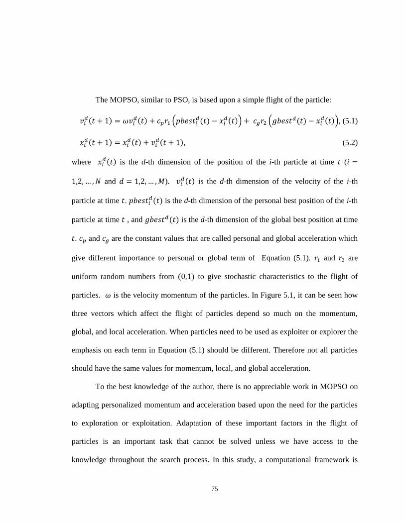
75

The MOPSO, similar to PSO, is based upon a simple flight of the particle:

, (5.1)

, (5.2)

where is the d-th dimension of the position of the i-th particle at time (

and ). is the d-th dimension of the velocity of the i-th

particle at time . is the d-th dimension of the personal best position of the i-th

particle at time , and is the d-th dimension of the global best position at time

. and are the constant values that are called personal and global acceleration which

give different importance to personal or global term of Equation (5.1). and are

uniform random numbers from to give stochastic characteristics to the flight of

particles. is the velocity momentum of the particles. In Figure 5.1, it can be seen how

three vectors which affect the flight of particles depend so much on the momentum,

global, and local acceleration. When particles need to be used as exploiter or explorer the

emphasis on each term in Equation (5.1) should be different. Therefore not all particles

should have the same values for momentum, local, and global acceleration.

To the best knowledge of the author, there is no appreciable work in MOPSO on

adapting personalized momentum and acceleration based upon the need for the particles

to exploration or exploitation. Adaptation of these important factors in the flight of

particles is an important task that cannot be solved unless we have access to the

knowledge throughout the search process. In this study, a computational framework is

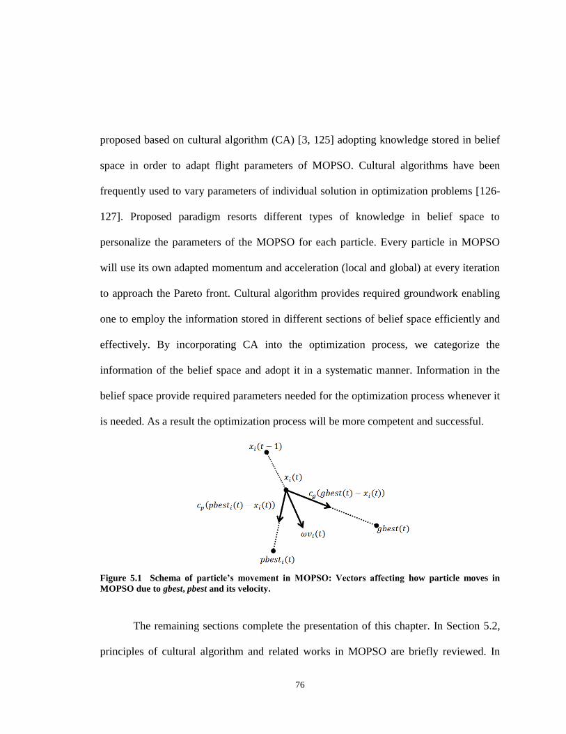
76

proposed based on cultural algorithm (CA) [3, 125] adopting knowledge stored in belief

space in order to adapt flight parameters of MOPSO. Cultural algorithms have been

frequently used to vary parameters of individual solution in optimization problems [126-

127]. Proposed paradigm resorts different types of knowledge in belief space to

personalize the parameters of the MOPSO for each particle. Every particle in MOPSO

will use its own adapted momentum and acceleration (local and global) at every iteration

to approach the Pareto front. Cultural algorithm provides required groundwork enabling

one to employ the information stored in different sections of belief space efficiently and

effectively. By incorporating CA into the optimization process, we categorize the

information of the belief space and adopt it in a systematic manner. Information in the

belief space provide required parameters needed for the optimization process whenever it

is needed. As a result the optimization process will be more competent and successful.

Figure 5.1 Schema of particle’s movement in MOPSO: Vectors affecting how particle moves in

MOPSO due to gbest, pbest and its velocity.

The remaining sections complete the presentation of this chapter. In Section 5.2,

principles of cultural algorithm and related works in MOPSO are briefly reviewed. In

77

Section 5.3, the proposed cultural MOPSO is elaborated. In Section 5.4, simulation

results are evaluated on the benchmark test problems in comparison with the state-of-the-

art MOPSO models. This section also includes a sensitivity analysis for the proposed

cultural MOPSO. Finally, Section 5.5 summarizes the concluding remarks and future

work of this study.

5.2 Review of Literature

5.2.1 Related Works in Multiobjective PSO

Hu and Eberhart [54] in their dynamic neighborhood MOPSO model and also Hu

et al. [66] in the MOPSO with extended memory adopted a random number on the range

(0.5,1) as the varying momentum, however both personal and global acceleration are

constant values. Sierra and Coello Coello [62] in their crowding and -dominance based

MOPSO used random value at the range (0.1,0.5) for the momentum and random values

at the range (1.5,2.0) for the personal and global acceleration. They adopted this scheme

to bypass the difficulties of fine tuning these parameters for each test function.

Zhang et al. [64] introduced intelligent MOPSO based upon Agent-Environment-

Rules model of artificial life. In their model, along with adopting some immunity clonal

operator, the momentum was decreased linearly from 0.6 to 0.2, but the personal and

global acceleration remained constant. Li [67] proposed an MOPSO based upon max-min

78

fitness function. In his model, while the personal and global accelerations were set

constant, the momentum was gradually decreased from 1.0 to 0.4. Zhang et al. [68]

adopted a linearly-decreasing momentum from 0.8 to 0.4 for their MOPSO algorithm.

However the personal and global accelerations were kept fixed values.

Mahfouf et al. [69] introduced adaptive weighted MOPSO in which they included

adaptive momentum and acceleration. Using comparison study with other well-behaved

algorithms, they demonstrated that the proposed MOPSO search capability is enhanced

by adding this adaptation. Ho et al. [63] noted the possible problem of selecting personal

and global acceleration independently and randomly. He mentioned because of its

stochastic nature they may both be too large or too small. In the former case, both

personal and global experiences are overused and as a result the particle will be driven

too far away from the optimum. For the latter case, both personal and global experiences

are underused and as a result the convergence speed of the algorithm is reduced. They

used sociobiological activity such as hunting to state that individuals balance between the

weight of their own knowledge and the group’s collective knowledge. In other words, the

personal and global acceleration are somehow related to each other. When one

acceleration is large, the other one should be small, and vice versa. Using this concept,

they modified the main equation of PSO, Equation (5.1), to include a dependent

acceleration and momentum [63].

It is a common belief that the need from every particle is different; they may need

larger or smaller momentum, depending on which part of search process they are located.

79

They also need to have different emphasis on personal or global term in Equation (5.1) of

MOPSO. Differentiated individual is a concept supported in the sociobiological studies

[7]. As a result of differentiation, individuals perform functions more efficiently.

5.2.2 Related Work in Cultural Algorithm for Multiobjective Optimization

Cultural algorithm is an adaptive evolutionary computation method which is

motivated by cultural evolution and learning in agent-based societies [3, 99]. CA consists

of evolving agents whose experiences are gathered into a belief space consisting of

various forms of symbolic knowledge. CA has shown its ability to solve different types

of problems [3, 99-107] among which CAEP (cultural algorithm along with evolutionary

programming) has shown successful results in solving MOPs [107]. Researchers have

identified five basic sections of knowledge stored in belief space based upon the literature

in cognitive science and semiotics: situational knowledge, normative knowledge,

topographical knowledge [105], domain knowledge, and history knowledge [106]. The

knowledge can swarm between different sections of belief space [108-110] which in turn

affect the swarming of population. Furthermore, cultural algorithm has shown its ability

[126-127] to optimize the control parameter of the optimization problem throughout the

search process. In order to adjust the parameters of MOPSO, we need to store several

types of required information, adopt this information in a proper manner, and update this

data properly. All these needs can be satisfied by implementing cultural algorithm. CA

provides groundwork for information repository through its belief space, use this

80

information by applying influence function to the knowledge space, and finally update

the population and belief space simultaneously.

5.3 Cultural-based Multiobjective Particle Swarm Optimization

A summary of the pseudocode of the proposed algorithm is shown in Figure 5.2

and a block diagram of the algorithm is also shown in Figure 5.3. The population space

(PSO) and its correspondent belief space (BLF) will be initialized at first. Then

population space is evaluated using the fitness values. We apply acceptance function to

select some particles which will be used to update belief space that consists of three

sections: situational, normative, and topographical knowledge in the current version of

implementation. Next we apply influence function and the belief space to adapt the

parameters of the PSO for next iteration such as global acceleration, local acceleration,

and momentum. We also use information on the belief space to select global best and

personal best for next iteration. Afterward, particles in population space fly using

personal and global best and newly adjusted momentum, local, and global acceleration.

This process continues until the stopping criteria are met.

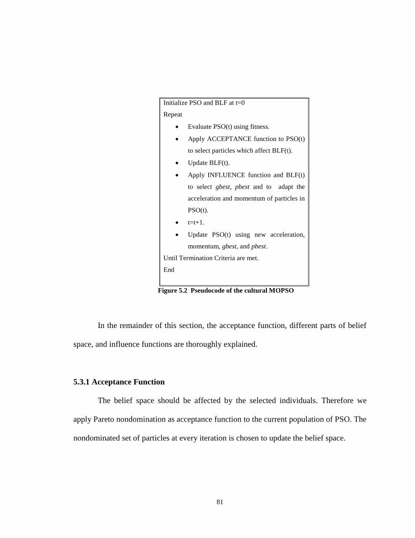
81

Initialize PSO and BLF at t=0

Repeat

Evaluate PSO(t) using fitness.

Apply ACCEPTANCE function to PSO(t)

to select particles which affect BLF(t).

Update BLF(t).

Apply INFLUENCE function and BLF(t)

to select gbest, pbest and to adapt the

acceleration and momentum of particles in

PSO(t).

t=t+1.

Update PSO(t) using new acceleration,

momentum, gbest, and pbest.

Until Termination Criteria are met.

End

Figure 5.2 Pseudocode of the cultural MOPSO

In the remainder of this section, the acceptance function, different parts of belief

space, and influence functions are thoroughly explained.

5.3.1 Acceptance Function

The belief space should be affected by the selected individuals. Therefore we

apply Pareto nondomination as acceptance function to the current population of PSO. The

nondominated set of particles at every iteration is chosen to update the belief space.

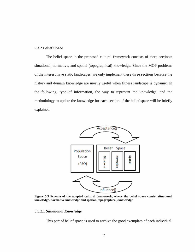
82

5.3.2 Belief Space

The belief space in the proposed cultural framework consists of three sections:

situational, normative, and spatial (topographical) knowledge. Since the MOP problems

of the interest have static landscapes, we only implement these three sections because the

history and domain knowledge are mostly useful when fitness landscape is dynamic. In

the following, type of information, the way to represent the knowledge, and the

methodology to update the knowledge for each section of the belief space will be briefly

explained.

Figure 5.3 Schema of the adopted cultural framework, where the belief space consist situational

knowledge, normative knowledge and spatial (topographical) knowledge

5.3.2.1 Situational Knowledge

This part of belief space is used to archive the good exemplars of each individual.

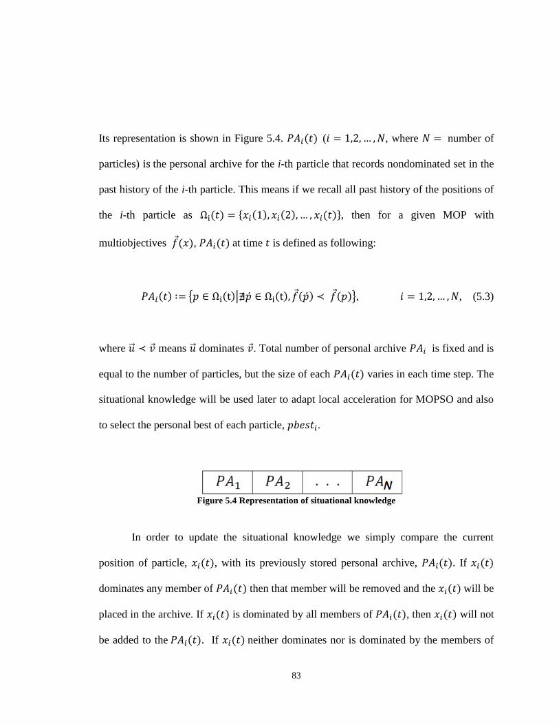
83

Its representation is shown in Figure 5.4. ( , where number of

particles) the personal archive for the i-th particle that records nondominated set in the

past history of the i-th particle. This means if we recall all past history of the positions of

the i-th particle as , then for a given MOP with

multiobjectives , at time is defined as following:

, , (5.3)

where means dominates . Total number of personal archive is fixed and is

equal to the number of particles, but the size of each varies in each time step. The

situational knowledge will be used later to adapt local acceleration for MOPSO and also

to select the personal best of each particle, .

Figure 5.4 Representation of situational knowledge

In order to update the situational knowledge we simply compare the current

position of particle, , with its previously stored personal archive, . If

dominates any member of then that member will be removed and the will be

placed in the archive. If is dominated by all members of , then will not

be added to the . If neither dominates nor is dominated by the members of

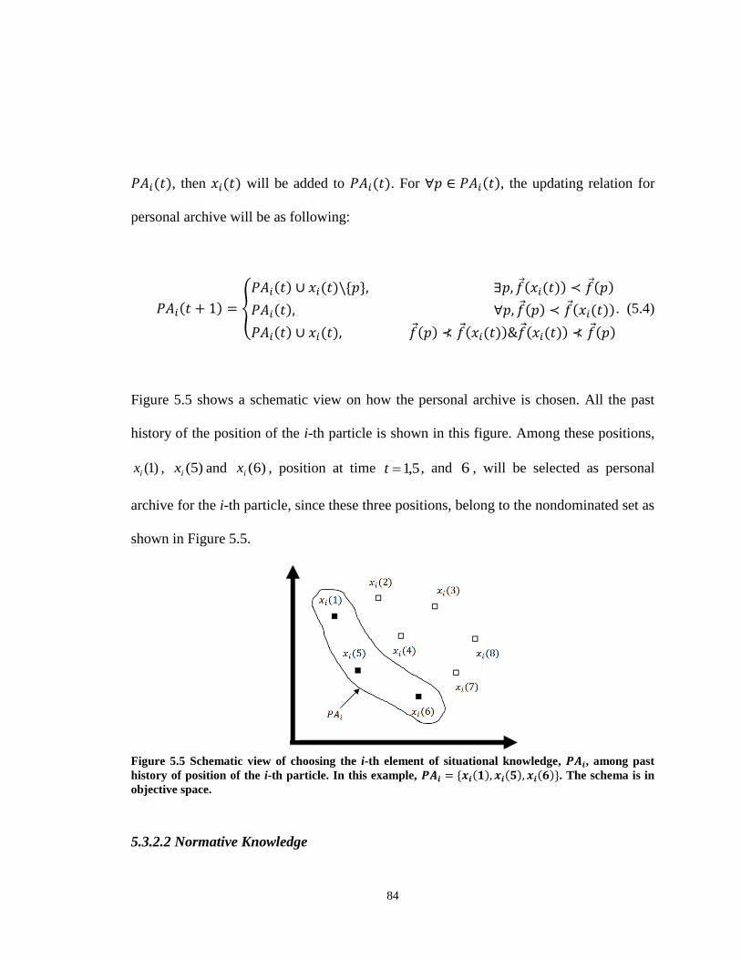
84

, then will be added to . For , the updating relation for

personal archive will be as following:

. (5.4)

Figure 5.5 shows a schematic view on how the personal archive is chosen. All the past

history of the position of the i-th particle is shown in this figure. Among these positions,

)1(ix , )5(ix and )6(ix , position at time 5,1t , and 6 , will be selected as personal

archive for the i-th particle, since these three positions, belong to the nondominated set as

shown in Figure 5.5.

Figure 5.5 Schematic view of choosing the i-th element of situational knowledge, , among past

history of position of the i-th particle. In this example, . The schema is in

objective space.

5.3.2.2 Normative Knowledge

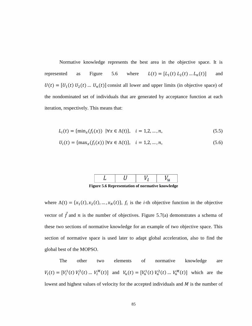
85

Normative knowledge represents the best area in the objective space. It is

represented as Figure 5.6 where and

consist all lower and upper limits (in objective space) of

the nondominated set of individuals that are generated by acceptance function at each

iteration, respectively. This means that:

, , (5.5)

, , (5.6)

Figure 5.6 Representation of normative knowledge

where , is the i-th objective function in the objective

vector of and is the number of objectives. Figure 5.7(a) demonstrates a schema of

these two sections of normative knowledge for an example of two objective space. This

section of normative space is used later to adapt global acceleration, also to find the

global best of the MOPSO.

The other two elements of normative knowledge are

and

which are the

lowest and highest values of velocity for the accepted individuals and is the number of

86

decision space variables:

, , (5.7)

, . (5.8)

.

This section of the normative knowledge is later used to adapt momentum of the

MOPSO. The normative knowledge is updated at each iteration based upon new

nondominated set as follows (assuming all objectives are based on minimization

problem).

, (5.9)

, (5.10)

where and are members of the nondominated set at time , . Figure

5.7(b) shows the updating process of this section of normative knowledge. Note

and . Furthermore, and will be updated using the

minimum and maximum velocities of the new set of nondominated individuals.

5.3.2.3 Topographical Knowledge

87

In order to represent topographical knowledge, we adopt the normative

knowledge and then divide the space into grids of where is the

number of division in the i-th dimension of objective space, and is the number of

objectives. Each of the resultant cells will then be represented as shown in Figure 5.8

where and consist all lower and upper limits

of the corresponding cell respectively, and is the number of nondominated

individuals of the whole population located on that cell:

, , , (5.11)

, , (5.12)

.

where and are given in Equations (5.5) and (5.6). Figure 5.9 demonstrates an

example on how a cell will be represented.

At every iteration, the topographic knowledge will be updated. To do so, updated

normative knowledge will be used to rebuild the cells and the nondominated points will

be counted in each cell. Topographical knowledge will be used later to adapt global

acceleration and also to find the global best, .

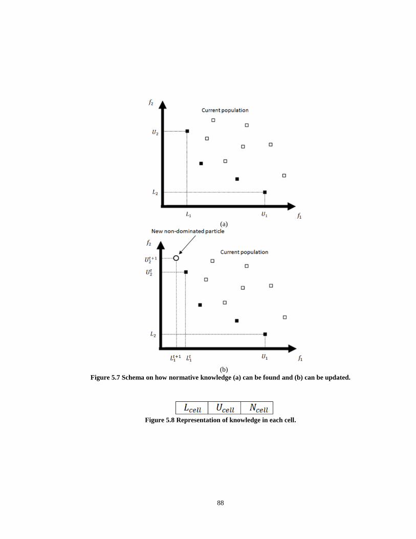
88

(a)

(b)

Figure 5.7 Schema on how normative knowledge (a) can be found and (b) can be updated.

Figure 5.8 Representation of knowledge in each cell.

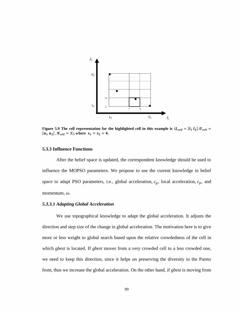
89

Figure 5.9 The cell representation for the highlighted cell in this example is , where .

5.3.3 Influence Functions

After the belief space is updated, the correspondent knowledge should be used to

influence the MOPSO parameters. We propose to use the current knowledge in belief

space to adapt PSO parameters, i.e., global acceleration, , local acceleration, , and

momentum, .

5.3.3.1 Adapting Global Acceleration

We use topographical knowledge to adapt the global acceleration. It adjusts the

direction and step size of the change in global acceleration. The motivation here is to give

more or less weight to global search based upon the relative crowdedness of the cell in

which gbest is located. If gbest moves from a very crowded cell to a less crowded one,

we need to keep this direction, since it helps on preserving the diversity in the Pareto

front, thus we increase the global acceleration. On the other hand, if gbest is moving from

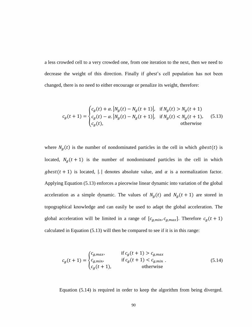
90

a less crowded cell to a very crowded one, from one iteration to the next, then we need to

decrease the weight of this direction. Finally if gbest’s cell population has not been

changed, there is no need to either encourage or penalize its weight, therefore:

, (5.13)

where is the number of nondominated particles in the cell in which is

located, is the number of nondominated particles in the cell in which

is located, denotes absolute value, and is a normalization factor.

Applying Equation (5.13) enforces a piecewise linear dynamic into variation of the global

acceleration as a simple dynamic. The values of and are stored in

topographical knowledge and can easily be used to adapt the global acceleration. The

global acceleration will be limited in a range of . Therefore

calculated in Equation (5.13) will then be compared to see if it is in this range:

. (5.14)

Equation (5.14) is required in order to keep the algorithm from being diverged.

91

We need to clarify that in regular MOPSO, is remained constant in Equation (5.1),

.

5.3.3.2 Adapting Local Acceleration

We use situational knowledge to build local grids in order to adjust local

acceleration. We adjust the direction and the step size of the change in local acceleration.

The procedure is similar to the one adopted for global acceleration. However in this case,

we use the personal archive stored in the situational knowledge of the belief space.

Therefore for each particle there will be different adjustment for its local acceleration

based on the relative crowdedness of the cell in which is located. For each

particle, we use its personal archive to build a local grid in order to find out the relative

crowdedness of the from one iteration to the next. In Figure 5.10, a schema shows

how a local grid is made using the situational knowledge for the i-th and j-th particle.

Each particle decides whether to increase or decrease its local acceleration

separately based upon its personal archive. If the particle is moving from a less crowded

cell to a more crowded one, we penalize its direction by decreasing the weight for local

acceleration and if the particle is moving from a more crowded cell to a less crowded

one, we need to keep that direction, thus increasing the weight for the local acceleration.

However, if there is no change in crowdedness of the particle’s cell, we should neither

increase nor decrease the local acceleration. Thus:

92

, (5.15)

where is the number of nondominated particles located in the same cell of local

grid of the i-th particle as , is the number of nondominated particles

located in the same cell of local grid of the i-th particle as , denotes

absolute value, and is a normalization factor. Piecewise linear behavior in Equation

(5.15) imposes a simple dynamic to variation of the local acceleration. The local

acceleration will also be restricted within a range of . That means

calculated in Equation (5.15) will then be checked to see if it is in this range:

. (5.16)

Equation (5.16) is also required in order to keep the algorithm from being

diverged. We also need to clarify in regular MOPSO, is kept constant in Equation

(5.1), .

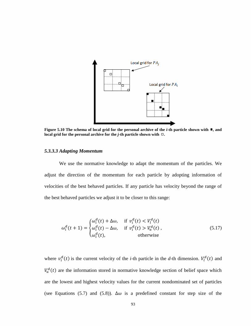
93

Figure 5.10 The schema of local grid for the personal archive of the i-th particle shown with , and

local grid for the personal archive for the j-th particle shown with .

5.3.3.3 Adapting Momentum

We use the normative knowledge to adapt the momentum of the particles. We

adjust the direction of the momentum for each particle by adopting information of

velocities of the best behaved particles. If any particle has velocity beyond the range of

the best behaved particles we adjust it to be closer to this range:

, (5.17)

where is the current velocity of the i-th particle in the d-th dimension.

and

are the information stored in normative knowledge section of belief space which

are the lowest and highest velocity values for the current nondominated set of particles

(see Equations (5.7) and (5.8)). is a predefined constant for step size of the

94

momentum. is the velocity momentum for the i-th particle in the d-th dimension.

The momentum needs to be limited in a range of to keep the algorithm

from being diverged. That means calculated in Equation (5.17) will need to be

compared to see if it is in this range:

. (5.18)

Finally we need to clarify that in regular MOPSO, Equation (5.1),

.

5.3.3.4 Selection

We use the topographical knowledge stored in belief space to select gbest at each

iteration. The method is borrowed from [58] which is based on selecting one

nondominated point located in the least populated area of the objective space. We use

roulette wheel selection to choose the appropriate cell which is more likely to be the least

populated cell and then randomly choose a particle from that cell to be global leader of

the particles. Each cell is assigned a fitness as [58]:

, (5.19)

where is the number of nondominated points located in that specific cell.

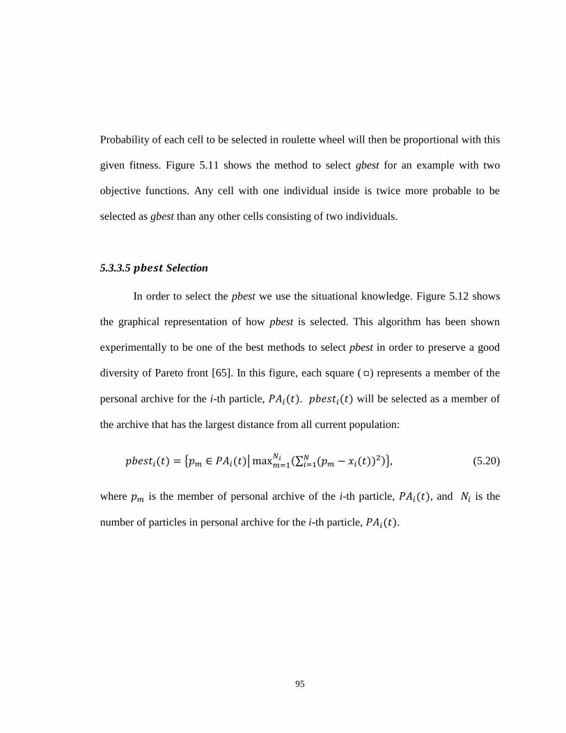
95

Probability of each cell to be selected in roulette wheel will then be proportional with this

given fitness. Figure 5.11 shows the method to select gbest for an example with two

objective functions. Any cell with one individual inside is twice more probable to be

selected as gbest than any other cells consisting of two individuals.

5.3.3.5 Selection

In order to select the pbest we use the situational knowledge. Figure 5.12 shows

the graphical representation of how pbest is selected. This algorithm has been shown

experimentally to be one of the best methods to select pbest in order to preserve a good

diversity of Pareto front [65]. In this figure, each square ( ) represents a member of the

personal archive for the i-th particle, . will be selected as a member of

the archive that has the largest distance from all current population:

, (5.20)

where is the member of personal archive of the i-th particle, , and is the

number of particles in personal archive for the i-th particle, .

96

Figure 5.11 Method of selecting from topographical knowledge.

5.3.4 Global Archive

We preserve the best solution into a global archive which is limited in size. To

update the global archive, each new nondominated solution will be compared with all

members in the archive. This method is the same as method explained in [58]. If a new

solution ( ) dominates any member of the global archive ( ) then that member will be

deleted and will be placed in the archive. If is dominated by all members of the

archive, then will be disregarded. If neither dominates nor is dominated by the

members of the archive, then there will be two scenarios. If the size of the archive does

not exceed the limit, the will be added to the archive. However, if the archive is already

full, then will be added to the archive and another member which is located in the most

populated area of the objective space will be deleted.

For , the updating relation for global archive after receiving any new

solution, , will be as following:

97

,

(5.21)

where is the current size of global archive, is the maximum size of global

archive, and is located in the most populated area. To find , we take advantage of

grid structure using the members of global archive and then locate the most populated

cell from that grid. will then be randomly selected from that cell and deleted.

Figure 5.12 selection procedure from personal archive: The for particle xi is selected

among the set of personal archive, PAi, in the objective space.

98

5.3.5 Time-decaying Mutation Operator

Due to tendency of immature convergence to local optima in PSO, a modified

version of a mutation operator introduced in [58] is proposed for the particles which are

not accepted through the acceptance function. The percentage of mutated particles, ,

is defined as following:

, (5.22)

where is the mutation rate ( ), is the current iteration and is the final iteration.

Adopting this form of mutation helps to scan a diverse region in the space at the

beginning of the search process. As current time, t, increases, the percentage of the

mutated particles approach to zero. This time-decaying mutation occurs in three ways:

(1) The number of particles that undergo the mutation is equal to:

, (5.23)

where is the number of dominated particles at the current iteration which are not

accepted through the acceptance function. These particles will be selected randomly.

(2) The range of mutation for each mutated particle will be time-decaying. For the d-th

dimension of the particle, , this range is defined as follows:

, (5.24)

where and

are the upper and lower limits of the particle in the d-th dimension.

The mutated particle will then be a random number in the range of .

Incorporating the time-decaying MP into this equation results a wider search range for

99

every mutated particle at the beginning of the search. As the iteration increases, the

search range for the mutated particle will be narrower.

(3) The mutation will happen for some dimensions of the selected particle. The number

of dimensions of those selected particles is time-decaying as following:

, (5.25)

where is the number of decision variables and is the rounding operator. Similarly,

incorporating MP into the number of dimensions for mutation will give one the benefit of

having more number of dimensions to be mutated at the beginning of the search, while it

approaches zero, as we reach the end of the process. These dimensions will be selected

randomly.

In this design, in the beginning, most particles in the population are subjected to

mutation (as well as the full range of the decision variables). This intends to produce a

highly explorative behavior in the algorithm. As the number of iterations increases, the

effect of the mutation decays.

5.4 Comparative Study and Sensitivity Analysis

This section consists of two experiments. In the first experiment, the performance

of the cultural MOPSO is evaluated against selected MOPSOs, while the second

experiment tests the sensitivity of the proposed algorithm with respect to its tuning

parameters.

100

5.4.1 Comparison Experiment

In this experiment, five state-of-the-art MOPSOs have been chosen in order to

compare their performance with that of the cultural MOPSO: sigma MOPSO [60],

OMOPSO [62], NSPSO [57], cluster MOPSO [128] and MOPSO [58].

5.4.1.1 Parameter Settings

Each of the six algorithms used here perform 200 iterations (as suggested in most

publications), and the archive size used is 100. The parameter settings for all of the

MOPSOs are summarized in Table 5.1. All of the algorithms are implemented in Matlab

using real-number representation for decision variables. However, binary representation

of decision variables can also be adopted. For each experiment, 100 independent runs

were conducted to collect the statistical results. All algorithms produced final Pareto

fronts of fixed size population except for cluster MOPSO, which does not have a fixed

archive size.

5.4.1.2 Benchmark Test Functions

To evaluate the performance of Cultural MOPSO against selected MOPSOs, six

benchmark test problems are used [129-130]: ZDT1, ZDT2, ZDT3, ZDT4, DTLZ5, and

DTLZ6.

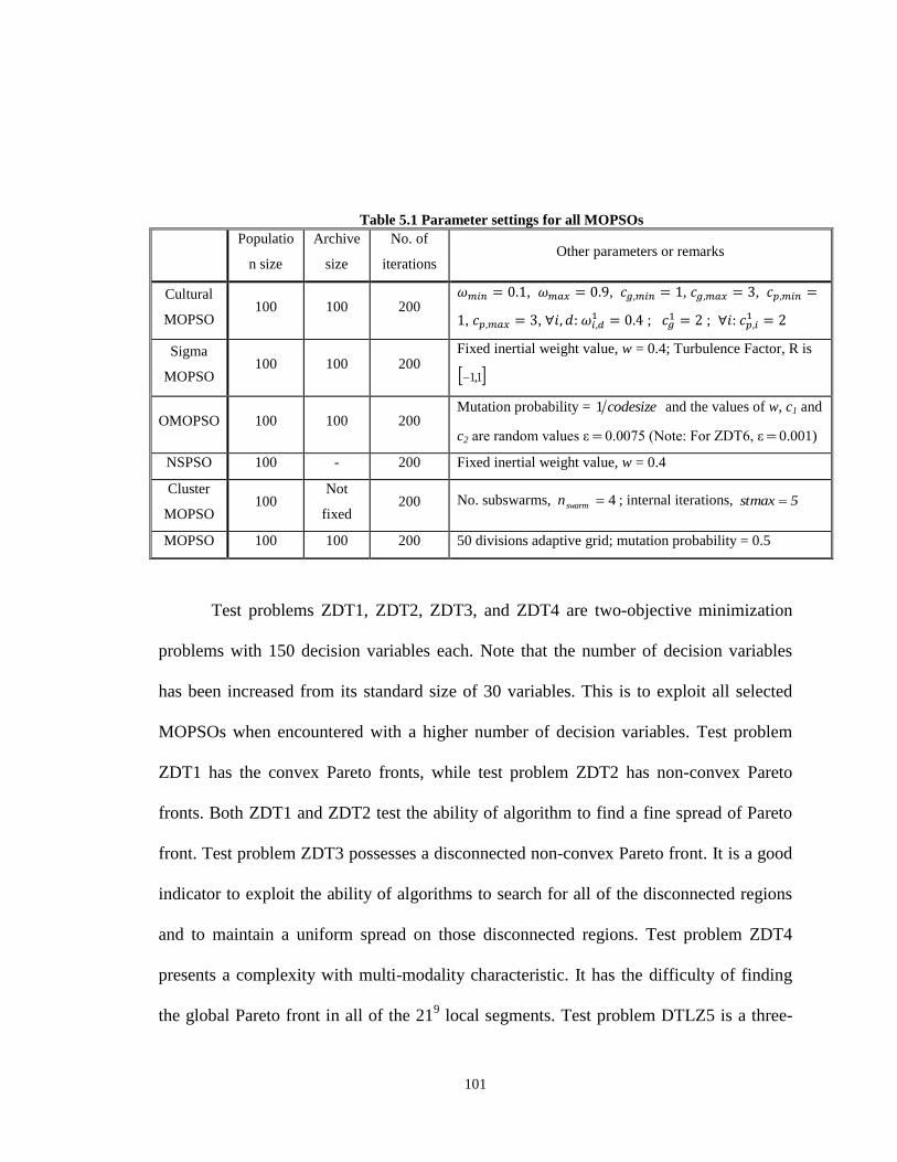
101

Table 5.1 Parameter settings for all MOPSOs

Populatio

n size

Archive

size

No. of

iterations Other parameters or remarks

Cultural

MOPSO 100 100 200

, , , ,

, , ;

;

Sigma

MOPSO 100 100 200

Fixed inertial weight value, w = 0.4; Turbulence Factor, R is

1,1

OMOPSO 100 100 200 Mutation probability = codesize1 and the values of w, c1 and

c2 are random values ε 0.0075 (Note: For ZDT6, ε 0.001)

NSPSO 100 - 200 Fixed inertial weight value, w = 0.4

Cluster

MOPSO 100

Not

fixed 200 No. subswarms, 4swarmn ; internal iterations, 5maxst

MOPSO 100 100 200 50 divisions adaptive grid; mutation probability = 0.5

Test problems ZDT1, ZDT2, ZDT3, and ZDT4 are two-objective minimization

problems with 150 decision variables each. Note that the number of decision variables

has been increased from its standard size of 30 variables. This is to exploit all selected

MOPSOs when encountered with a higher number of decision variables. Test problem

ZDT1 has the convex Pareto fronts, while test problem ZDT2 has non-convex Pareto

fronts. Both ZDT1 and ZDT2 test the ability of algorithm to find a fine spread of Pareto

front. Test problem ZDT3 possesses a disconnected non-convex Pareto front. It is a good

indicator to exploit the ability of algorithms to search for all of the disconnected regions

and to maintain a uniform spread on those disconnected regions. Test problem ZDT4

presents a complexity with multi-modality characteristic. It has the difficulty of finding

the global Pareto front in all of the 219 local segments. Test problem DTLZ5 is a three-

102

objective minimization problem with 150 decision variable. Note that the number of

decision variables has been increased from its standard size of 12. This is again to exploit

all MOSPOs when encountered with a higher number of decision variables. DTLZ5 has a

three dimensional curve as Pareto front located on the surface of the unit sphere. Its

difficulty is that the density of solutions closer to the Pareto front curve becomes much

less than anywhere else in the search space. Test problem DTLZ6, a three-objective

minimization problem with 22 decision variables, has four disconnected set of Pareto

front regions. This problem tests an algorithm’s ability to maintain subpopulation in

multiple Pareto-optimal regions. The detailed formulation of these benchmark test

functions are presented in Appendix A for reference.

5.4.1.3 Qualitative Performance Comparisons

For qualitative comparison, the plots of final Pareto fronts are presented for

visualization. The resulted nondominated fronts (given the same initial population from a

single run) of the six MOPSOs on all test functions are demonstrated in Figures 5.13 to

5.18. These figures show cultural MOPSO is able to find the well-extended, near-optimal

Pareto fronts despite a very large number of decision variables for test functions ZDT1 to

ZDT4 and DTLZ5. MOPSO [58] provides the second best results, where it can produce

fine Pareto fronts similar to the ones produced by cultural MOPSO for most benchmark

test functions. Cluster MOPSO, sigma MOPSO, and NSPSO produce the worst Pareto

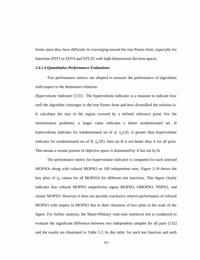
103

fronts since they have difficulty in converging toward the true Pareto front, especially for

functions ZDT1 to ZDT4 and DTLZ5 with high-dimensional decision spaces.

5.4.1.4 Quantitative Performance Evaluations

Two performance metrics are adopted to measure the performance of algorithms

with respect to the dominance relations.

Hypervolume Indicator [131]: The hypervolume indicator is a measure to indicate how

well the algorithm converges to the true Pareto front and how diversified the solution is.

It calculates the size of the region covered by a defined reference point. For the

minimization problems, a larger value indicates a better nondominated set. If

hypervolume indicator for nondominated set of , , is greater than hypervolume

indicator for nondominated set of , , then set B is not better than A for all pairs.

This means a certain portion of objective space is dominated by A but not by B.

The performance metric for hypervolume indicator is computed for each selected

MOPSOs along with cultural MOPSO on 100 independent runs. Figure 5.19 shows the

box plots of values for all MOPSOs for different test functions. This figure clearly

indicates that cultural MOPSO outperforms sigma MOPSO, OMOPSO, NSPSO, and

cluster MOPSO. However it does not provide conclusive relative performance of cultural

MOPSO with respect to MOPSO due to their closeness of box plots in the scale of the

figure. For further analysis, the Mann-Whitney rank-sum statistical test is conducted to

evaluate the significant difference between two independent samples for all pairs [132]

and the results are illustrated in Table 5.2. In this table, for each test function and each

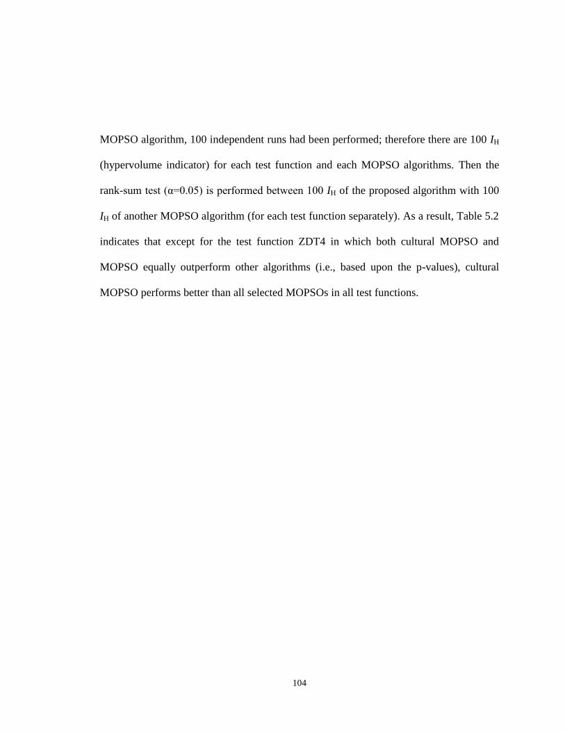
104

MOPSO algorithm, 100 independent runs had been performed; therefore there are 100 IH

(hypervolume indicator) for each test function and each MOPSO algorithms. Then the

rank-sum test (α=0.05) is performed between 100 IH of the proposed algorithm with 100

IH of another MOPSO algorithm (for each test function separately). As a result, Table 5.2

indicates that except for the test function ZDT4 in which both cultural MOPSO and

MOPSO equally outperform other algorithms (i.e., based upon the p-values), cultural

MOPSO performs better than all selected MOPSOs in all test functions.

105

(a) (b)

(c) (d)

(e) (f)

Figure 5.13 Pareto fronts produced by (a) cultural MOPSO, (b) sigma MOPSO, (c) OMOPSO, (d)

NSPSO, (e) cluster MOPSO, and (f) MOPSO on test function ZDT1.

0 0.1 0.2 0.3 0.4 0.5 0.6 0.7 0.8 0.9 10

0.2

0.4

0.6

0.8

1

1.2

1.4

0 0.1 0.2 0.3 0.4 0.5 0.6 0.7 0.8 0.9 10

0.5

1

1.5

2

2.5

0 0.1 0.2 0.3 0.4 0.5 0.6 0.7 0.8 0.9 10

0.5

1

1.5

0 0.1 0.2 0.3 0.4 0.5 0.6 0.7 0.8 0.9 10

0.5

1

1.5

2

2.5

3

3.5

4

0 0.1 0.2 0.3 0.4 0.5 0.6 0.7 0.8 0.9 10

0.2

0.4

0.6

0.8

1

1.2

1.4

0 0.1 0.2 0.3 0.4 0.5 0.6 0.7 0.8 0.9 10

0.1

0.2

0.3

0.4

0.5

0.6

0.7

0.8

0.9

1

106

(a) (b)

(c) (d)

(e) (f)



0 0.1 0.2 0.3 0.4 0.5 0.6 0.7 0.8 0.9 10

0.2

0.4

0.6

0.8

1

1.2

1.4

0 0.1 0.2 0.3 0.4 0.5 0.6 0.7 0.8 0.9 10

0.2

0.4

0.6

0.8

1

1.2

1.4

1.6

1.8

2

0 0.1 0.2 0.3 0.4 0.5 0.6 0.7 0.8 0.9 10

0.2

0.4

0.6

0.8

1

1.2

1.4

0 0.1 0.2 0.3 0.4 0.5 0.6 0.7 0.8 0.9 10

0.5

1

1.5

2

2.5

3

3.5

0 0.1 0.2 0.3 0.4 0.5 0.6 0.7 0.8 0.9 10

0.2

0.4

0.6

0.8

1

1.2

1.4

1.6

1.8

0 0.1 0.2 0.3 0.4 0.5 0.6 0.7 0.8 0.9 10

0.2

0.4

0.6

0.8

1

1.2

1.4

107

(a) (b)

(c) (d)

(e) (f)



0 0.1 0.2 0.3 0.4 0.5 0.6 0.7 0.8 0.9 1-0.8

-0.6

-0.4

-0.2

0

0.2

0.4

0.6

0.8

1

1.2

0 0.1 0.2 0.3 0.4 0.5 0.6 0.7 0.8 0.9 1-1

-0.5

0

0.5

1

1.5

2

2.5

0 0.1 0.2 0.3 0.4 0.5 0.6 0.7 0.8 0.9 1-1

-0.5

0

0.5

1

1.5

2

0 0.1 0.2 0.3 0.4 0.5 0.6 0.7 0.8 0.9 1-1

-0.5

0

0.5

1

1.5

2

2.5

3

3.5

0 0.1 0.2 0.3 0.4 0.5 0.6 0.7 0.8 0.9 1-1

-0.5

0

0.5

1

1.5

2

0 0.1 0.2 0.3 0.4 0.5 0.6 0.7 0.8 0.9 1-0.8

-0.6

-0.4

-0.2

0

0.2

0.4

0.6

0.8

1

1.2

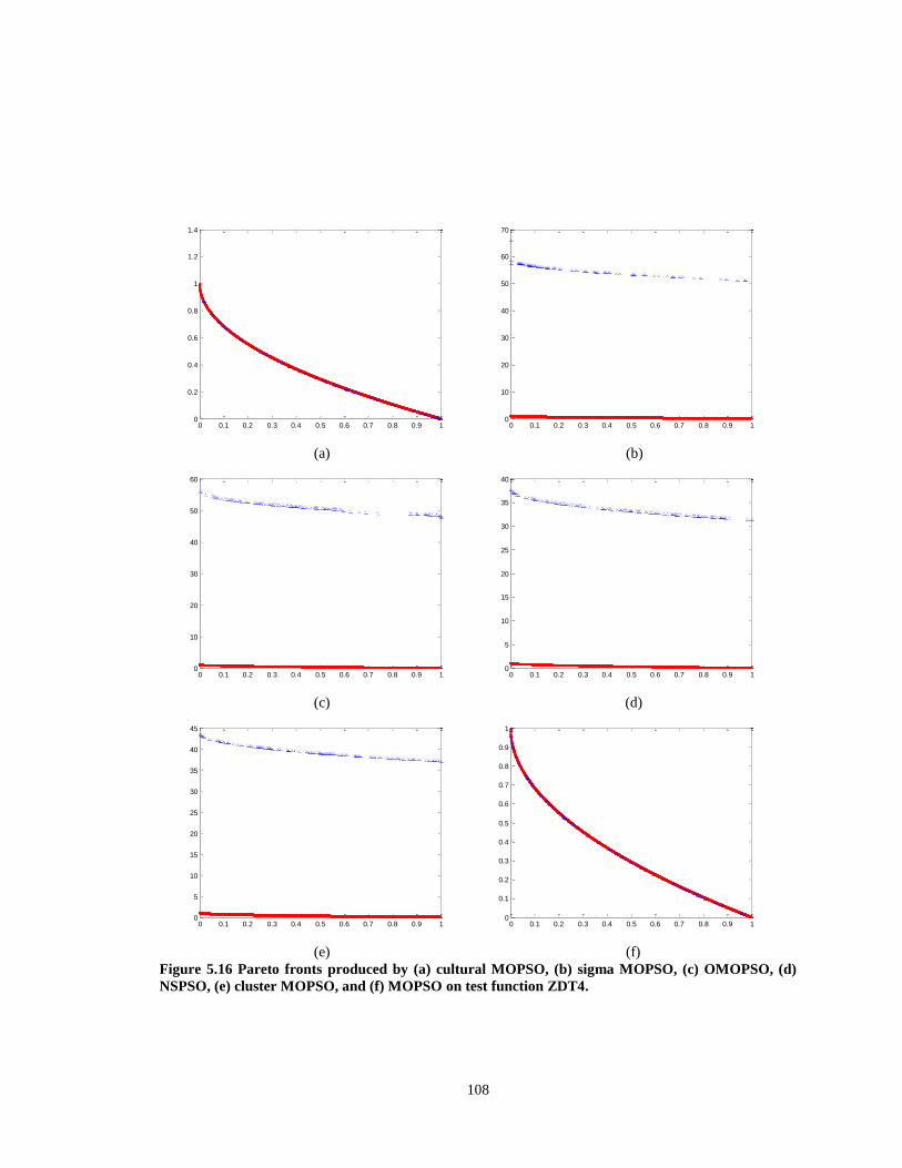
108

(a) (b)

(c) (d)

(e) (f)



0 0.1 0.2 0.3 0.4 0.5 0.6 0.7 0.8 0.9 10

0.2

0.4

0.6

0.8

1

1.2

1.4

0 0.1 0.2 0.3 0.4 0.5 0.6 0.7 0.8 0.9 10

10

20

30

40

50

60

70

0 0.1 0.2 0.3 0.4 0.5 0.6 0.7 0.8 0.9 10

10

20

30

40

50

60

0 0.1 0.2 0.3 0.4 0.5 0.6 0.7 0.8 0.9 10

5

10

15

20

25

30

35

40

0 0.1 0.2 0.3 0.4 0.5 0.6 0.7 0.8 0.9 10

5

10

15

20

25

30

35

40

45

0 0.1 0.2 0.3 0.4 0.5 0.6 0.7 0.8 0.9 10

0.1

0.2

0.3

0.4

0.5

0.6

0.7

0.8

0.9

1

109

(a) (b)

(c) (d)

(e) (f)


NSPSO, (e) cluster MOPSO, and (f) MOPSO on test function DTLZ5.

0

0.2

0.4

0.6

0.8 0

0.2

0.4

0.6

0.8

0

0.2

0.4

0.6

0.8

1

0

50

100 0

20

40

60

80

0

20

40

60

80

0

20

40

60

80 0

20

40

60

80

0

20

40

60

80

0

50

100 020

4060

80100

0

20

40

60

80

0

20

40

60

80 0

20

40

60

80

0

10

20

30

40

50

60

0

0.5

1

1.5 0

0.5

1

1.5

0

0.5

1

1.5

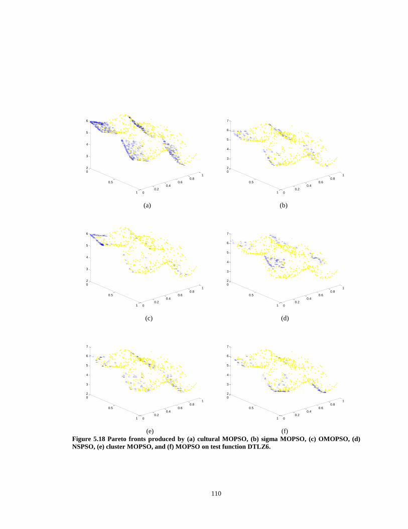
110

(a) (b)

(c) (d)

(e) (f)


NSPSO, (e) cluster MOPSO, and (f) MOPSO on test function DTLZ6.

0

0.5

1 00.2

0.40.6

0.81

2

3

4

5

6

0

0.5

1 00.2

0.40.6

0.81

2

3

4

5

6

7

0

0.5

1 00.2

0.40.6

0.81

2

3

4

5

6

0

0.5

1 00.2

0.40.6

0.81

2

3

4

5

6

7

0

0.5

1 00.2

0.40.6

0.81

2

3

4

5

6

7

0

0.5

1 00.2

0.40.6

0.81

2

3

4

5

6

7

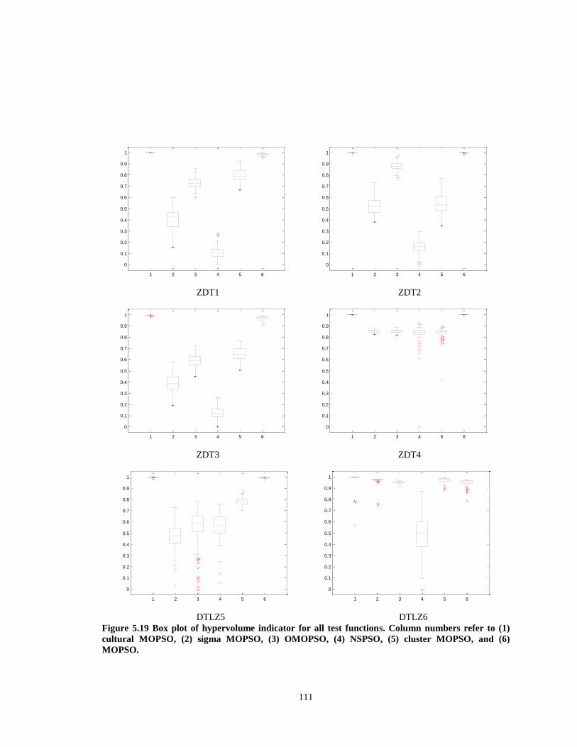
111

ZDT1 ZDT2

ZDT3 ZDT4

DTLZ5 DTLZ6

Figure 5.19 Box plot of hypervolume indicator for all test functions. Column numbers refer to (1)

cultural MOPSO, (2) sigma MOPSO, (3) OMOPSO, (4) NSPSO, (5) cluster MOPSO, and (6)

MOPSO.

1 2 3 4 5 6

0

0.1

0.2

0.3

0.4

0.5

0.6

0.7

0.8

0.9

1

1 2 3 4 5 6

0

0.1

0.2

0.3

0.4

0.5

0.6

0.7

0.8

0.9

1

1 2 3 4 5 6

0

0.1

0.2

0.3

0.4

0.5

0.6

0.7

0.8

0.9

1

1 2 3 4 5 6

0

0.1

0.2

0.3

0.4

0.5

0.6

0.7

0.8

0.9

1

1 2 3 4 5 6

0

0.1

0.2

0.3

0.4

0.5

0.6

0.7

0.8

0.9

1

1 2 3 4 5 6

0

0.1

0.2

0.3

0.4

0.5

0.6

0.7

0.8

0.9

1

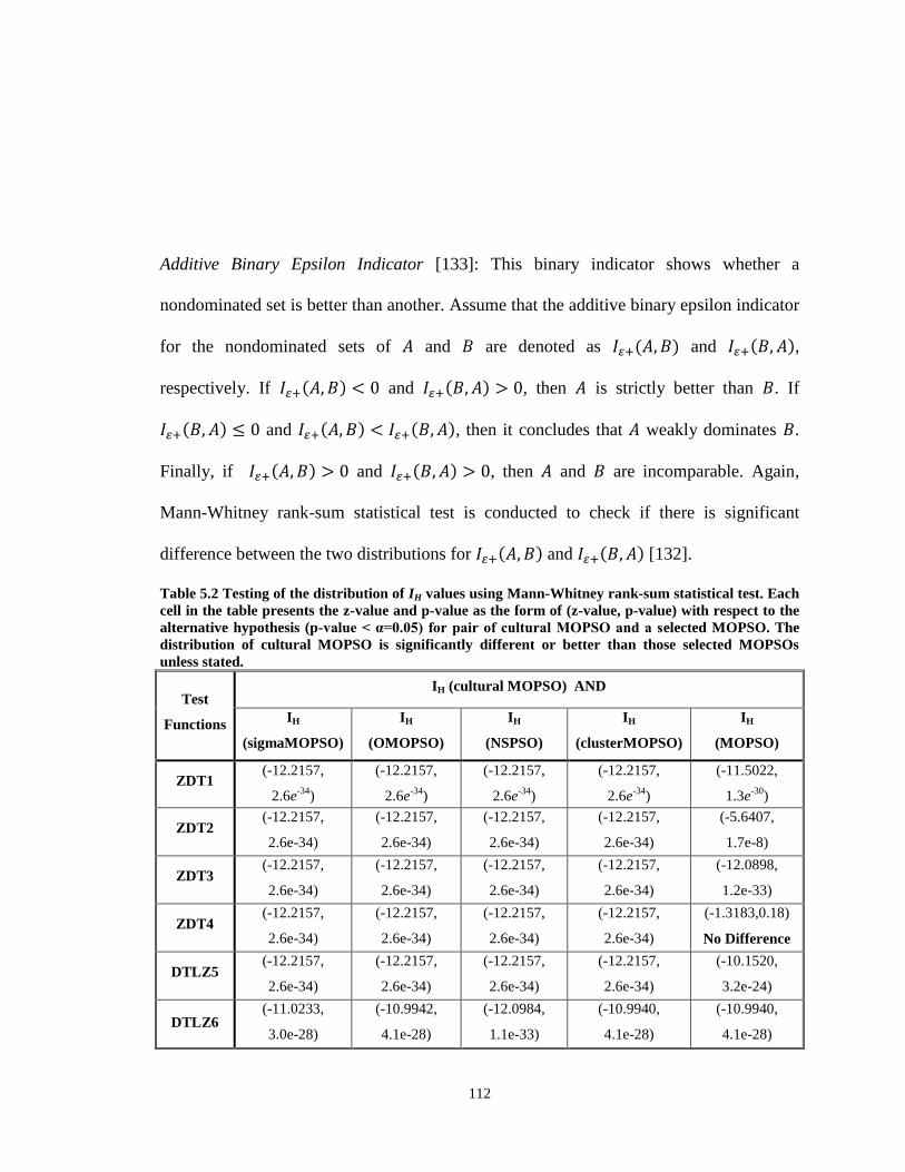
112

Additive Binary Epsilon Indicator [133]: This binary indicator shows whether a

nondominated set is better than another. Assume that the additive binary epsilon indicator

for the nondominated sets of and are denoted as and ,

respectively. If and , then is strictly better than . If

and , then it concludes that weakly dominates .

Finally, if and , then and are incomparable. Again,

Mann-Whitney rank-sum statistical test is conducted to check if there is significant

difference between the two distributions for and [132].

Table 5.2 Testing of the distribution of IH values using Mann-Whitney rank-sum statistical test. Each

cell in the table presents the z-value and p-value as the form of (z-value, p-value) with respect to the

alternative hypothesis (p-value < α=0.05) for pair of cultural MOPSO and a selected MOPSO. The

distribution of cultural MOPSO is significantly different or better than those selected MOPSOs

unless stated.

Test

Functions

IH (cultural MOPSO) AND

IH

(sigmaMOPSO)

IH

(OMOPSO)

IH

(NSPSO)

IH

(clusterMOPSO)

IH

(MOPSO)

ZDT1 (-12.2157,

2.6e-34

)

(-12.2157,

2.6e-34

)

(-12.2157,

2.6e-34

)

(-12.2157,

2.6e-34

)

(-11.5022,

1.3e-30

)

ZDT2 (-12.2157,

2.6e-34)

(-12.2157,

2.6e-34)

(-12.2157,

2.6e-34)

(-12.2157,

2.6e-34)

(-5.6407,

1.7e-8)

ZDT3 (-12.2157,

2.6e-34)

(-12.2157,

2.6e-34)

(-12.2157,

2.6e-34)

(-12.2157,

2.6e-34)

(-12.0898,

1.2e-33)

ZDT4 (-12.2157,

2.6e-34)

(-12.2157,

2.6e-34)

(-12.2157,

2.6e-34)

(-12.2157,

2.6e-34)

(-1.3183,0.18)

No Difference

DTLZ5 (-12.2157,

2.6e-34)

(-12.2157,

2.6e-34)

(-12.2157,

2.6e-34)

(-12.2157,

2.6e-34)

(-10.1520,

3.2e-24)

DTLZ6 (-11.0233,

3.0e-28)

(-10.9942,

4.1e-28)

(-12.0984,

1.1e-33)

(-10.9940,

4.1e-28)

(-10.9940,

4.1e-28)

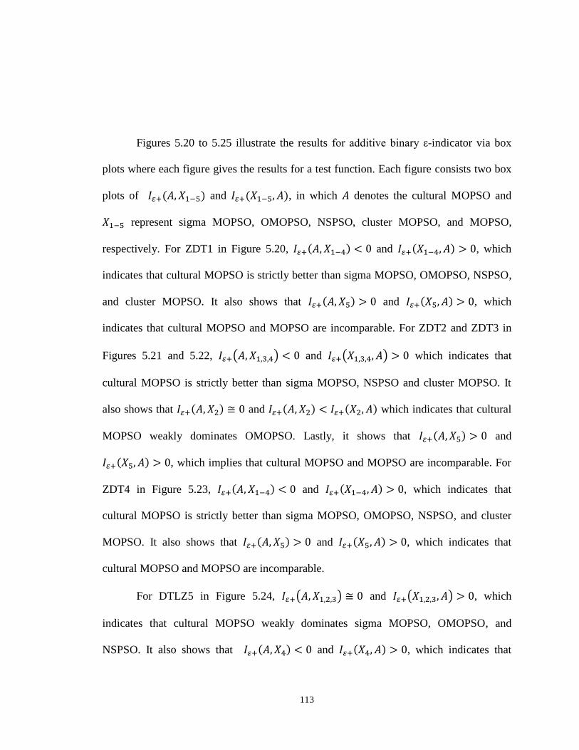
113

Figures 5.20 to 5.25 illustrate the results for additive binary ε-indicator via box

plots where each figure gives the results for a test function. Each figure consists two box

plots of and , in which denotes the cultural MOPSO and

represent sigma MOPSO, OMOPSO, NSPSO, cluster MOPSO, and MOPSO,

respectively. For ZDT1 in Figure 5.20, and , which

indicates that cultural MOPSO is strictly better than sigma MOPSO, OMOPSO, NSPSO,

and cluster MOPSO. It also shows that and , which

indicates that cultural MOPSO and MOPSO are incomparable. For ZDT2 and ZDT3 in

Figures 5.21 and 5.22, and which indicates that

cultural MOPSO is strictly better than sigma MOPSO, NSPSO and cluster MOPSO. It

also shows that and which indicates that cultural

MOPSO weakly dominates OMOPSO. Lastly, it shows that and

, which implies that cultural MOPSO and MOPSO are incomparable. For

ZDT4 in Figure 5.23, and , which indicates that

cultural MOPSO is strictly better than sigma MOPSO, OMOPSO, NSPSO, and cluster

MOPSO. It also shows that and , which indicates that

cultural MOPSO and MOPSO are incomparable.

For DTLZ5 in Figure 5.24, and , which

indicates that cultural MOPSO weakly dominates sigma MOPSO, OMOPSO, and

NSPSO. It also shows that and , which indicates that

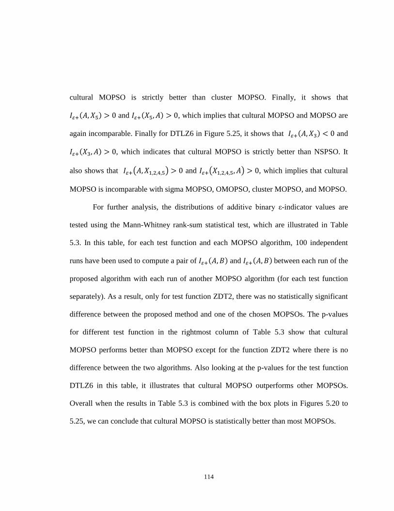
114

cultural MOPSO is strictly better than cluster MOPSO. Finally, it shows that

and , which implies that cultural MOPSO and MOPSO are

again incomparable. Finally for DTLZ6 in Figure 5.25, it shows that and

, which indicates that cultural MOPSO is strictly better than NSPSO. It

also shows that and , which implies that cultural

MOPSO is incomparable with sigma MOPSO, OMOPSO, cluster MOPSO, and MOPSO.

For further analysis, the distributions of additive binary ε-indicator values are

tested using the Mann-Whitney rank-sum statistical test, which are illustrated in Table

5.3. In this table, for each test function and each MOPSO algorithm, 100 independent

runs have been used to compute a pair of and between each run of the

proposed algorithm with each run of another MOPSO algorithm (for each test function

separately). As a result, only for test function ZDT2, there was no statistically significant

difference between the proposed method and one of the chosen MOPSOs. The p-values

for different test function in the rightmost column of Table 5.3 show that cultural

MOPSO performs better than MOPSO except for the function ZDT2 where there is no

difference between the two algorithms. Also looking at the p-values for the test function

DTLZ6 in this table, it illustrates that cultural MOPSO outperforms other MOPSOs.

Overall when the results in Table 5.3 is combined with the box plots in Figures 5.20 to

5.25, we can conclude that cultural MOPSO is statistically better than most MOPSOs.

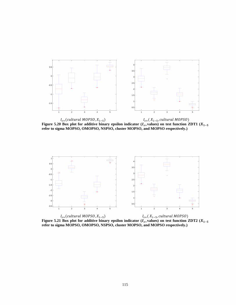
115

Figure 5.20 Box plot for additive binary epsilon indicator ( values) on test function ZDT1 (

refer to sigma MOPSO, OMOPSO, NSPSO, cluster MOPSO, and MOPSO respectively.)



1 2 3 4 5

-1.5

-1

-0.5

0

0.5

1 2 3 4 5

0.5

1

1.5

2

2.5

3

3.5

4

1 2 3 4 5

-3.5

-3

-2.5

-2

-1.5

-1

-0.5

0

0.5

1

1 2 3 4 5

0.5

1

1.5

2

2.5

3

3.5

4

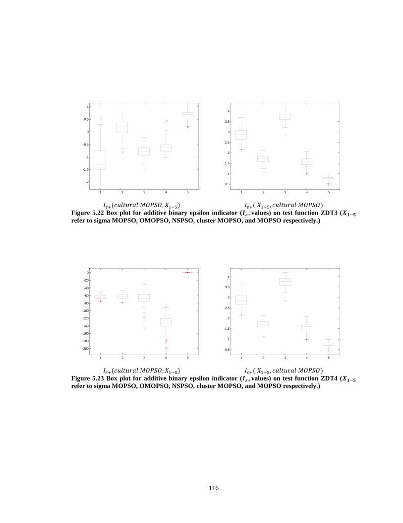
116





1 2 3 4 5

-2

-1.5

-1

-0.5

0

0.5

1

1 2 3 4 5

0.5

1

1.5

2

2.5

3

3.5

4

1 2 3 4 5

-200

-180

-160

-140

-120

-100

-80

-60

-40

-20

0

1 2 3 4 5

0.5

1

1.5

2

2.5

3

3.5

4

117

Figure 5.24 Box plot for additive binary epsilon indicator ( values) on test function DTLZ5 (


Figure 5.25 Box plot for additive binary epsilon indicator ( values) on test function DTLZ6 (


1 2 3 4 5

-60

-50

-40

-30

-20

-10

0

1 2 3 4 5

0.5

1

1.5

2

2.5

3

3.5

4

1 2 3 4 5

-4

-3

-2

-1

0

1

2

3

4

5

6

1 2 3 4 5

0.5

1

1.5

2

2.5

3

3.5

4

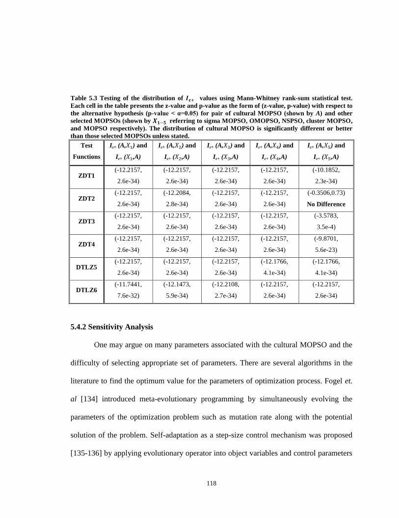
118

Table 5.3 Testing of the distribution of values using Mann-Whitney rank-sum statistical test.

Each cell in the table presents the z-value and p-value as the form of (z-value, p-value) with respect to

the alternative hypothesis (p-value < α=0.05) for pair of cultural MOPSO (shown by A) and other

selected MOPSOs (shown by referring to sigma MOPSO, OMOPSO, NSPSO, cluster MOPSO,

and MOPSO respectively). The distribution of cultural MOPSO is significantly different or better

than those selected MOPSOs unless stated.

Test

Functions

Iε+ (A, ) and

Iε+ ( ,A)

Iε+ (A, ) and

Iε+ ( ,A)

Iε+ (A, ) and

Iε+ ( ,A)

Iε+ (A, ) and

Iε+ ( ,A)

Iε+ (A, ) and

Iε+ ( ,A)

ZDT1 (-12.2157,

2.6e-34)

(-12.2157,

2.6e-34)

(-12.2157,

2.6e-34)

(-12.2157,

2.6e-34)

(-10.1852,

2.3e-34)

ZDT2 (-12.2157,

2.6e-34)

(-12.2084,

2.8e-34)

(-12.2157,

2.6e-34)

(-12.2157,

2.6e-34)

(-0.3506,0.73)

No Difference

ZDT3 (-12.2157,

2.6e-34)

(-12.2157,

2.6e-34)

(-12.2157,

2.6e-34)

(-12.2157,

2.6e-34)

(-3.5783,

3.5e-4)

ZDT4 (-12.2157,

2.6e-34)

(-12.2157,

2.6e-34)

(-12.2157,

2.6e-34)

(-12.2157,

2.6e-34)

(-9.8701,

5.6e-23)

DTLZ5 (-12.2157,

2.6e-34)

(-12.2157,

2.6e-34)

(-12.2157,

2.6e-34)

(-12.1766,

4.1e-34)

(-12.1766,

4.1e-34)

DTLZ6 (-11.7441,

7.6e-32)

(-12.1473,

5.9e-34)

(-12.2108,

2.7e-34)

(-12.2157,

2.6e-34)

(-12.2157,

2.6e-34)

5.4.2 Sensitivity Analysis

One may argue on many parameters associated with the cultural MOPSO and the

difficulty of selecting appropriate set of parameters. There are several algorithms in the

literature to find the optimum value for the parameters of optimization process. Fogel et.

al [134] introduced meta-evolutionary programming by simultaneously evolving the

parameters of the optimization problem such as mutation rate along with the potential

solution of the problem. Self-adaptation as a step-size control mechanism was proposed

[135-136] by applying evolutionary operator into object variables and control parameters

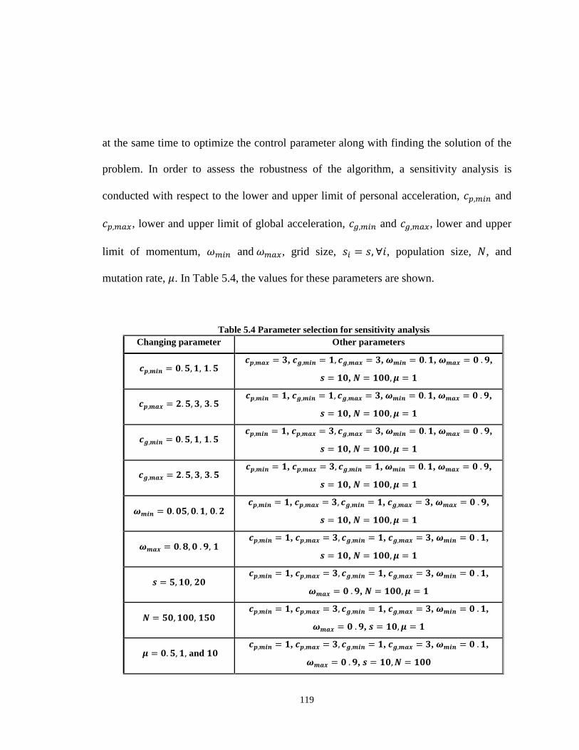
119

at the same time to optimize the control parameter along with finding the solution of the

problem. In order to assess the robustness of the algorithm, a sensitivity analysis is

conducted with respect to the lower and upper limit of personal acceleration, and

, lower and upper limit of global acceleration, and , lower and upper

limit of momentum, and , grid size, , population size, , and

mutation rate, . In Table 5.4, the values for these parameters are shown.

Table 5.4 Parameter selection for sensitivity analysis

Changing parameter Other parameters

, , , ,

,

, , , ,

,

, , , ,

,

, , , ,

,

, , , ,

,

, , , ,

,

, , , ,

,

, , , ,

,

and , , , ,

,

120

For each value of one chosen parameter, 30 independent runs of cultural MOPSO

were conducted. The additive binary epsilon indicator (Iε+ values) is used to compare the

Pareto set for each run. For example, to investigate the sensitivity of the algorithm with

respect to , three values of are adopted. After 30 independent

runs for the algorithm with each parameter setting on , we calculate ,

, , , , where and refer to algorithm

with and , respectively. Notice that for , each singe run of

is compared against every single run of . Then box plots for these six pairs are

constructed. Figures 5.26 to 5.34 show the box plot for all nine different parameters for

sensitivity analysis. For further analysis, Mann-Whitney rank-sum statistical test is

implemented to check if there is a significant difference between the two distributions for

and [132]. The results are displayed in Tables 5.5 to 5.13.

Figure 5.26 along with Table 5.5 demonstrate that by changing the lower limit of

personal acceleration, , for all test functions there is no significant difference

among the final Pareto fronts using different values of , except for the test function

DTLZ5 when comparing and , where and refer to algorithm

with and , respectively. Figure 5.27 along with Table 5.6 illustrates that

by changing the upper limit of personal acceleration, , for all test functions there is

no significant difference among the final Pareto fronts using different values of .

121

Figure 5.28 along with Table 5.7 demonstrate that by changing the lower limit of global

acceleration, , for all test functions there is no significant difference among the

final Pareto fronts using different values of , except for the test function ZDT2

when comparing and , and for test function DTLZ5 when comparing

and , where and refer to cultural MOPSO with

and , respectively. Figure 5.29 along with Table 5.8 illustrates that by

changing the upper limit of global acceleration, , for all test functions there is no

significant difference among the final Pareto fronts using different values of .

Figure 5.30 along with Table 5.9 demonstrate that by changing the lower limit of

momentum, , for all test functions there is no significant difference among the final

Pareto fronts using different values of , except for the test function ZDT4 when

comparing and , where and refer to algorithm with

and , respectively. Figure 5.31 along with Table 5.10 show that by changing the upper

limit of momentum, , for all test functions there is no significant difference among

the final Pareto fronts using different values of , except for the test function ZDT1

when comparing and , where and refer to algorithm with

and , respectively. Figure 5.32 along with Table 5.11 demonstrate that by

changing the grid size, , for all test functions there is no significant difference among the

final Pareto fronts using different values of , except for the test function ZDT1 when

comparing and , and test function DTLZ6 when comparing

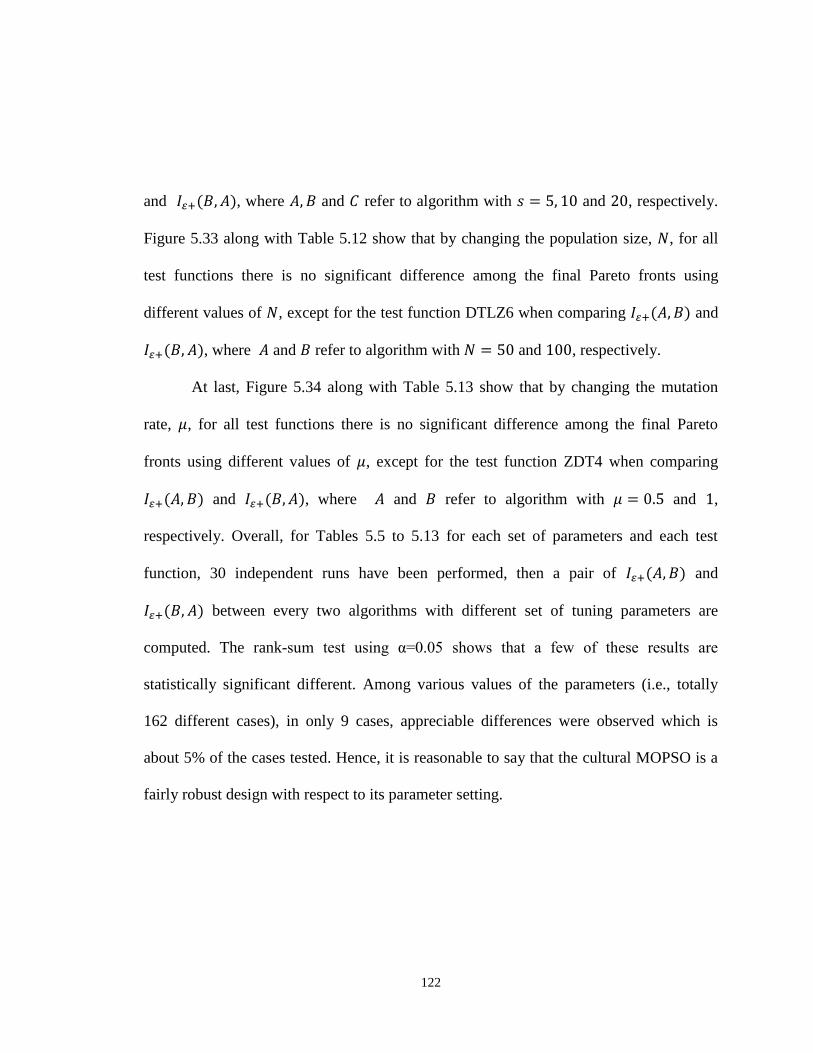
122

and , where and refer to algorithm with and , respectively.

Figure 5.33 along with Table 5.12 show that by changing the population size, , for all

test functions there is no significant difference among the final Pareto fronts using

different values of , except for the test function DTLZ6 when comparing and

, where and refer to algorithm with and , respectively.

At last, Figure 5.34 along with Table 5.13 show that by changing the mutation

rate, , for all test functions there is no significant difference among the final Pareto

fronts using different values of , except for the test function ZDT4 when comparing

and , where and refer to algorithm with and ,

respectively. Overall, for Tables 5.5 to 5.13 for each set of parameters and each test

function, 30 independent runs have been performed, then a pair of and

between every two algorithms with different set of tuning parameters are

computed. The rank-sum test using α=0.05 shows that a few of these results are

statistically significant different. Among various values of the parameters (i.e., totally

162 different cases), in only 9 cases, appreciable differences were observed which is

about 5% of the cases tested. Hence, it is reasonable to say that the cultural MOPSO is a

fairly robust design with respect to its parameter setting.

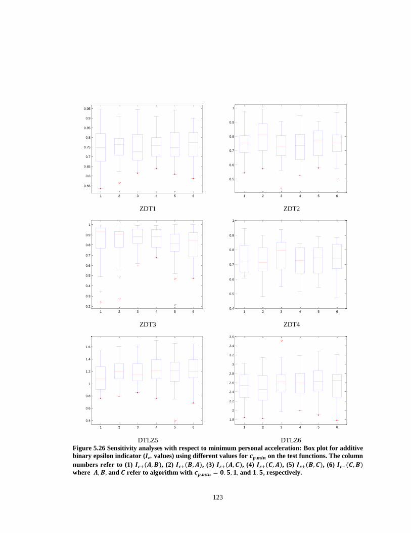
123

ZDT1 ZDT2

ZDT3 ZDT4

DTLZ5 DTLZ6

Figure 5.26 Sensitivity analyses with respect to minimum personal acceleration: Box plot for additive

binary epsilon indicator (Iε+ values) using different values for on the test functions. The column

numbers refer to (1) , (2) , (3) , (4) , (5) , (6)

where and refer to algorithm with and , respectively.

1 2 3 4 5 6

0.55

0.6

0.65

0.7

0.75

0.8

0.85

0.9

0.95

1 2 3 4 5 6

0.5

0.6

0.7

0.8

0.9

1

1 2 3 4 5 6

0.2

0.3

0.4

0.5

0.6

0.7

0.8

0.9

1

1 2 3 4 5 60.4

0.5

0.6

0.7

0.8

0.9

1

1 2 3 4 5 6

0.4

0.6

0.8

1

1.2

1.4

1.6

1 2 3 4 5 6

1.8

2

2.2

2.4

2.6

2.8

3

3.2

3.4

3.6

124

ZDT1 ZDT2

ZDT3 ZDT4

DTLZ5 DTLZ6

Figure 5.27 Sensitivity analyses with respect to maximum personal acceleration: Box plot for additive

binary epsilon indicator (Iε+ values) using different values for on the test functions. The

column numbers refer to (1) , (2) , (3) , (4) , (5) , (6)


1 2 3 4 5 6

0.5

0.55

0.6

0.65

0.7

0.75

0.8

0.85

0.9

0.95

1 2 3 4 5 6

0.4

0.5

0.6

0.7

0.8

0.9

1

1 2 3 4 5 6

0.3

0.4

0.5

0.6

0.7

0.8

0.9

1

1 2 3 4 5 60.45

0.5

0.55

0.6

0.65

0.7

0.75

0.8

0.85

0.9

0.95

1 2 3 4 5 6

0.6

0.8

1

1.2

1.4

1.6

1.8

1 2 3 4 5 6

1

1.5

2

2.5

3

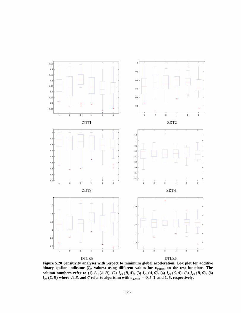
125

ZDT1 ZDT2

ZDT3 ZDT4

DTLZ5 DTLZ6

Figure 5.28 Sensitivity analyses with respect to minimum global acceleration: Box plot for additive




1 2 3 4 5 6

0.55

0.6

0.65

0.7

0.75

0.8

0.85

0.9

0.95

1 2 3 4 5 6

0.5

0.6

0.7

0.8

0.9

1

1 2 3 4 5 60.2

0.3

0.4

0.5

0.6

0.7

0.8

0.9

1

1 2 3 4 5 6

0.3

0.4

0.5

0.6

0.7

0.8

0.9

1

1.1

1 2 3 4 5 6

0.6

0.8

1

1.2

1.4

1.6

1 2 3 4 5 6

1.5

2

2.5

3

3.5

126

ZDT1 ZDT2

ZDT3 ZDT4

DTLZ5 DTLZ6

Figure 5.29 Sensitivity analyses with respect to maximum global acceleration: Box plot for additive




1 2 3 4 5 6

0.5

0.55

0.6

0.65

0.7

0.75

0.8

0.85

0.9

0.95

1 2 3 4 5 60.4

0.5

0.6

0.7

0.8

0.9

1

1 2 3 4 5 60.1

0.2

0.3

0.4

0.5

0.6

0.7

0.8

0.9

1

1 2 3 4 5 6

0.5

0.6

0.7

0.8

0.9

1

1.1

1.2

1.3

1.4

1 2 3 4 5 6

0.6

0.8

1

1.2

1.4

1.6

1 2 3 4 5 6

1

1.5

2

2.5

3

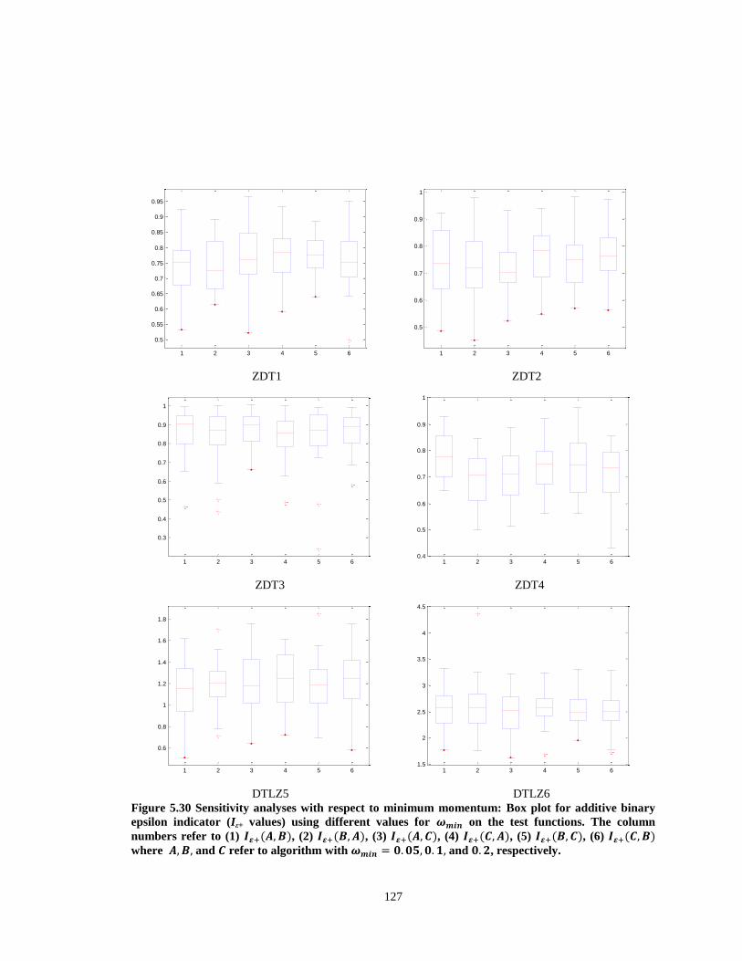
127

ZDT1 ZDT2

ZDT3 ZDT4

DTLZ5 DTLZ6

Figure 5.30 Sensitivity analyses with respect to minimum momentum: Box plot for additive binary

epsilon indicator (Iε+ values) using different values for on the test functions. The column

numbers refer to (1) , (2) , (3) , (4) , (5) , (6)


1 2 3 4 5 6

0.5

0.55

0.6

0.65

0.7

0.75

0.8

0.85

0.9

0.95

1 2 3 4 5 6

0.5

0.6

0.7

0.8

0.9

1

1 2 3 4 5 6

0.3

0.4

0.5

0.6

0.7

0.8

0.9

1

1 2 3 4 5 60.4

0.5

0.6

0.7

0.8

0.9

1

1 2 3 4 5 6

0.6

0.8

1

1.2

1.4

1.6

1.8

1 2 3 4 5 61.5

2

2.5

3

3.5

4

4.5

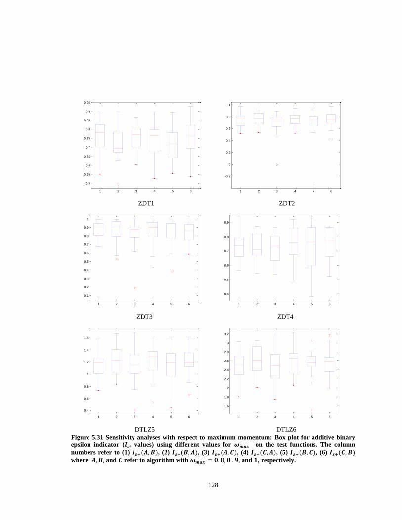
128

ZDT1 ZDT2

ZDT3 ZDT4

DTLZ5 DTLZ6

Figure 5.31 Sensitivity analyses with respect to maximum momentum: Box plot for additive binary

epsilon indicator (Iε+ values) using different values for on the test functions. The column

numbers refer to (1) , (2) , (3) , (4) , (5) , (6)


1 2 3 4 5 6

0.5

0.55

0.6

0.65

0.7

0.75

0.8

0.85

0.9

0.95

1 2 3 4 5 6

-0.2

0

0.2

0.4

0.6

0.8

1

1 2 3 4 5 6

0.1

0.2

0.3

0.4

0.5

0.6

0.7

0.8

0.9

1

1 2 3 4 5 6

0.4

0.5

0.6

0.7

0.8

0.9

1 2 3 4 5 6

0.4

0.6

0.8

1

1.2

1.4

1.6

1 2 3 4 5 6

1.6

1.8

2

2.2

2.4

2.6

2.8

3

3.2

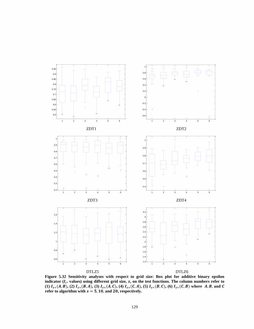
129

ZDT1 ZDT2

ZDT3 ZDT4

DTLZ5 DTLZ6

Figure 5.32 Sensitivity analyses with respect to grid size: Box plot for additive binary epsilon

indicator (Iε+ values) using different grid size, , on the test functions. The column numbers refer to

(1) , (2) , (3) , (4) , (5) , (6) where and

refer to algorithm with and , respectively.

1 2 3 4 5 6

0.5

0.55

0.6

0.65

0.7

0.75

0.8

0.85

0.9

0.95

1 2 3 4 5 6

-0.6

-0.4

-0.2

0

0.2

0.4

0.6

0.8

1

1 2 3 4 5 60.2

0.3

0.4

0.5

0.6

0.7

0.8

0.9

1

1 2 3 4 5 6

0.4

0.5

0.6

0.7

0.8

0.9

1

1 2 3 4 5 6

0.6

0.8

1

1.2

1.4

1.6

1 2 3 4 5 61.2

1.4

1.6

1.8

2

2.2

2.4

2.6

2.8

3

3.2

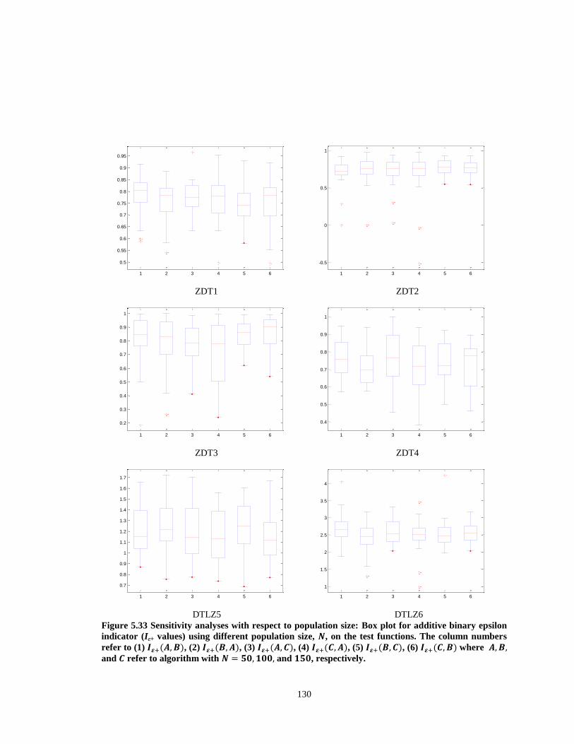
130

ZDT1 ZDT2

ZDT3 ZDT4

DTLZ5 DTLZ6

Figure 5.33 Sensitivity analyses with respect to population size: Box plot for additive binary epsilon

indicator (Iε+ values) using different population size, , on the test functions. The column numbers

refer to (1) , (2) , (3) , (4) , (5) , (6) where and refer to algorithm with and , respectively.

1 2 3 4 5 6

0.5

0.55

0.6

0.65

0.7

0.75

0.8

0.85

0.9

0.95

1 2 3 4 5 6

-0.5

0

0.5

1

1 2 3 4 5 6

0.2

0.3

0.4

0.5

0.6

0.7

0.8

0.9

1

1 2 3 4 5 6

0.4

0.5

0.6

0.7

0.8

0.9

1

1 2 3 4 5 6

0.7

0.8

0.9

1

1.1

1.2

1.3

1.4

1.5

1.6

1.7

1 2 3 4 5 6

1

1.5

2

2.5

3

3.5

4

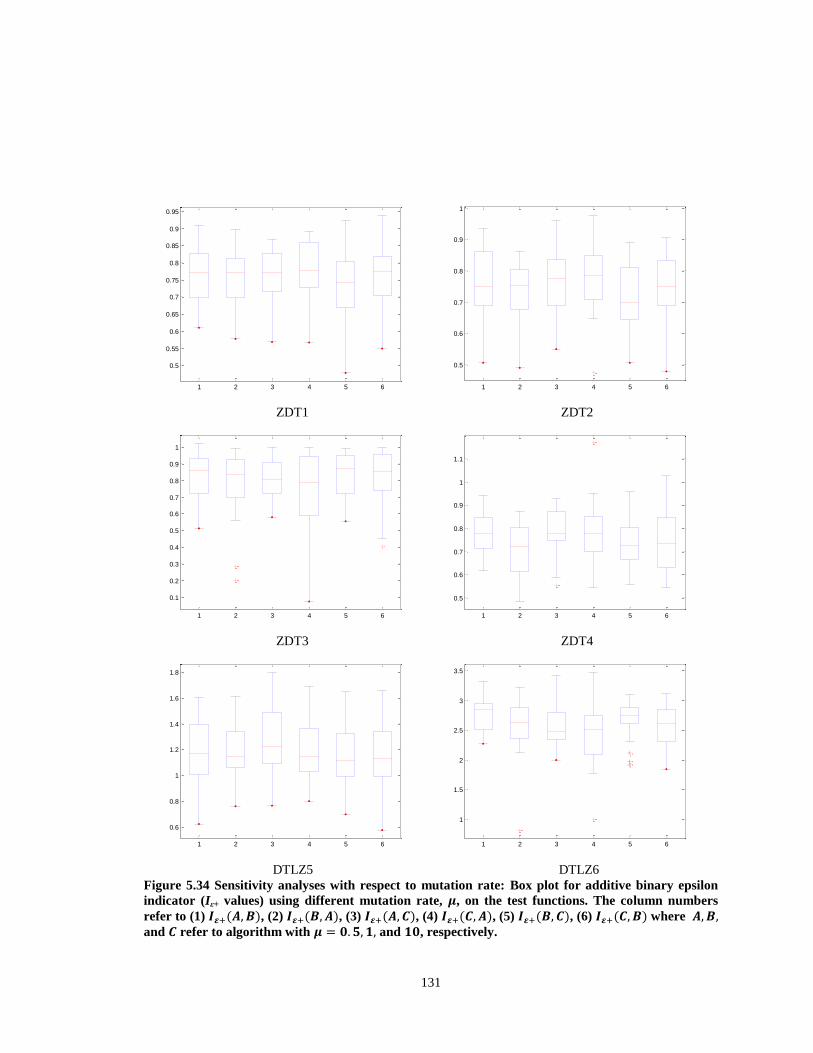
131

ZDT1 ZDT2

ZDT3 ZDT4

DTLZ5 DTLZ6

Figure 5.34 Sensitivity analyses with respect to mutation rate: Box plot for additive binary epsilon

indicator (Iε+ values) using different mutation rate, , on the test functions. The column numbers

refer to (1) , (2) , (3) , (4) , (5) , (6) where and refer to algorithm with and , respectively.

1 2 3 4 5 6

0.5

0.55

0.6

0.65

0.7

0.75

0.8

0.85

0.9

0.95

1 2 3 4 5 6

0.5

0.6

0.7

0.8

0.9

1

1 2 3 4 5 6

0.1

0.2

0.3

0.4

0.5

0.6

0.7

0.8

0.9

1

1 2 3 4 5 6

0.5

0.6

0.7

0.8

0.9

1

1.1

1 2 3 4 5 6

0.6

0.8

1

1.2

1.4

1.6

1.8

1 2 3 4 5 6

1

1.5

2

2.5

3

3.5

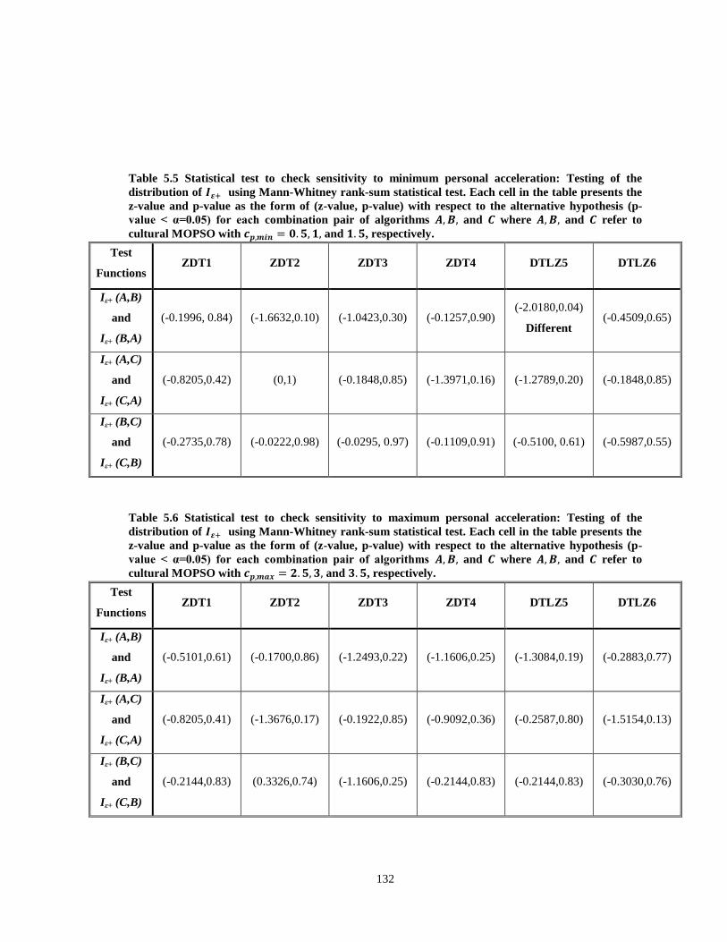
132

Table 5.5 Statistical test to check sensitivity to minimum personal acceleration: Testing of the

distribution of using Mann-Whitney rank-sum statistical test. Each cell in the table presents the

z-value and p-value as the form of (z-value, p-value) with respect to the alternative hypothesis (p-

value < α=0.05) for each combination pair of algorithms and where and refer to

cultural MOPSO with and , respectively.

Test

Functions ZDT1 ZDT2 ZDT3 ZDT4 DTLZ5 DTLZ6

Iε+ (A,B)

and

Iε+ (B,A)

(-0.1996, 0.84) (-1.6632,0.10) (-1.0423,0.30) (-0.1257,0.90) (-2.0180,0.04)

Different (-0.4509,0.65)

Iε+ (A,C)

and

Iε+ (C,A)

(-0.8205,0.42) (0,1) (-0.1848,0.85) (-1.3971,0.16) (-1.2789,0.20) (-0.1848,0.85)

Iε+ (B,C)

and

Iε+ (C,B)

(-0.2735,0.78) (-0.0222,0.98) (-0.0295, 0.97) (-0.1109,0.91) (-0.5100, 0.61) (-0.5987,0.55)

Table 5.6 Statistical test to check sensitivity to maximum personal acceleration: Testing of the





Test


Iε+ (A,B)

and

Iε+ (B,A)

(-0.5101,0.61) (-0.1700,0.86) (-1.2493,0.22) (-1.1606,0.25) (-1.3084,0.19) (-0.2883,0.77)

Iε+ (A,C)

and

Iε+ (C,A)

(-0.8205,0.41) (-1.3676,0.17) (-0.1922,0.85) (-0.9092,0.36) (-0.2587,0.80) (-1.5154,0.13)

Iε+ (B,C)

and

Iε+ (C,B)

(-0.2144,0.83) (0.3326,0.74) (-1.1606,0.25) (-0.2144,0.83) (-0.2144,0.83) (-0.3030,0.76)

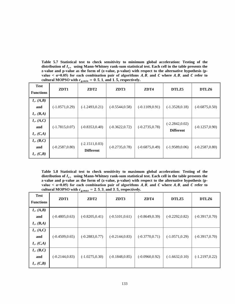
133

Table 5.7 Statistical test to check sensitivity to minimum global acceleration: Testing of the





Test


Iε+ (A,B)

and

Iε+ (B,A)

(-1.0571,0.29) (-1.2493,0.21) (-0.5544,0.58) (-0.1109,0.91) (-1.3528,0.18) (-0.6875,0.50)

Iε+ (A,C)

and

Iε+ (C,A)

(-1.7815,0.07) (-0.8353,0.40) (-0.3622,0.72) (-0.2735,0.78) (-2.2842,0.02)

Different (-0.1257,0.90)

Iε+ (B,C)

and

Iε+ (C,B)

(-0.2587,0.80) (-2.1511,0.03)

Different (-0.2735,0.78) (-0.6875,0.49) (-1.9589,0.06) (-0.2587,0.80)

Table 5.8 Statistical test to check sensitivity to maximum global acceleration: Testing of the





Test


Iε+ (A,B)

and

Iε+ (B,A)

(-0.4805,0.63) (-0.8205,0.41) (-0.5101,0.61) (-0.8649,0.39) (-0.2292,0.82) (-0.3917,0.70)

Iε+ (A,C)

and

Iε+ (C,A)

(-0.4509,0.65) (-0.2883,0.77) (-0.2144,0.83) (-0.3770,0.71) (-1.0571,0.29) (-0.3917,0.70)

Iε+ (B,C)

and

Iε+ (C,B)

(-0.2144,0.83) (-1.0275,0.30) (-0.1848,0.85) (-0.0960,0.92) (-1.6632,0.10) (-1.2197,0.22)

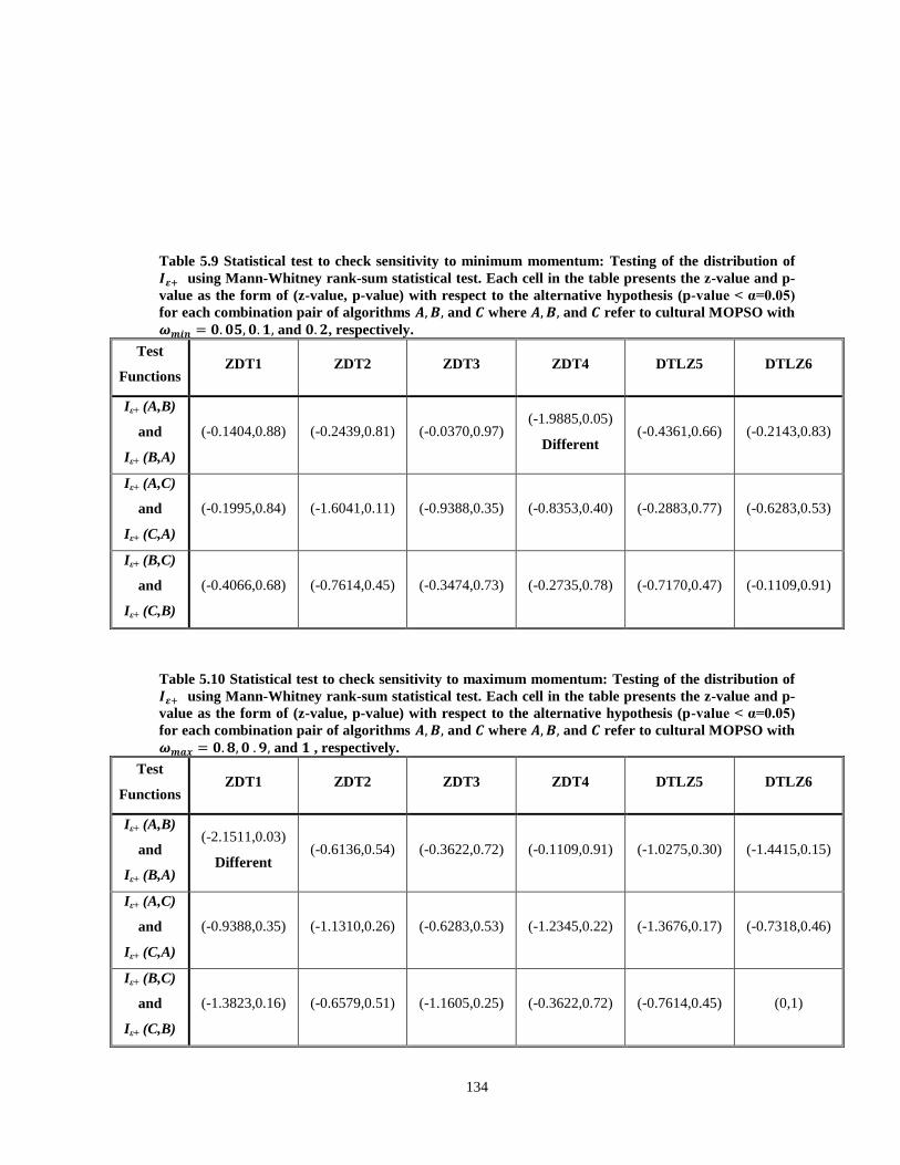
134

Table 5.9 Statistical test to check sensitivity to minimum momentum: Testing of the distribution of

using Mann-Whitney rank-sum statistical test. Each cell in the table presents the z-value and p-

value as the form of (z-value, p-value) with respect to the alternative hypothesis (p-value < α=0.05)

for each combination pair of algorithms and where and refer to cultural MOPSO with

and , respectively.

Test


Iε+ (A,B)

and

Iε+ (B,A)

(-0.1404,0.88) (-0.2439,0.81) (-0.0370,0.97) (-1.9885,0.05)

Different (-0.4361,0.66) (-0.2143,0.83)

Iε+ (A,C)

and

Iε+ (C,A)

(-0.1995,0.84) (-1.6041,0.11) (-0.9388,0.35) (-0.8353,0.40) (-0.2883,0.77) (-0.6283,0.53)

Iε+ (B,C)

and

Iε+ (C,B)

(-0.4066,0.68) (-0.7614,0.45) (-0.3474,0.73) (-0.2735,0.78) (-0.7170,0.47) (-0.1109,0.91)

Table 5.10 Statistical test to check sensitivity to maximum momentum: Testing of the distribution of

using Mann-Whitney rank-sum statistical test. Each cell in the table presents the z-value and p-

value as the form of (z-value, p-value) with respect to the alternative hypothesis (p-value < α=0.05)

for each combination pair of algorithms and where and refer to cultural MOPSO with

and , respectively.

Test


Iε+ (A,B)

and

Iε+ (B,A)

(-2.1511,0.03)

Different (-0.6136,0.54) (-0.3622,0.72) (-0.1109,0.91) (-1.0275,0.30) (-1.4415,0.15)

Iε+ (A,C)

and

Iε+ (C,A)

(-0.9388,0.35) (-1.1310,0.26) (-0.6283,0.53) (-1.2345,0.22) (-1.3676,0.17) (-0.7318,0.46)

Iε+ (B,C)

and

Iε+ (C,B)

(-1.3823,0.16) (-0.6579,0.51) (-1.1605,0.25) (-0.3622,0.72) (-0.7614,0.45) (0,1)

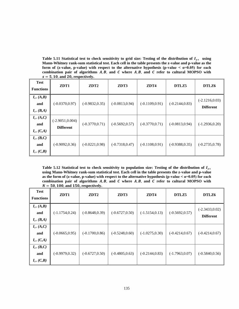
135

Table 5.11 Statistical test to check sensitivity to grid size: Testing of the distribution of using

Mann-Whitney rank-sum statistical test. Each cell in the table presents the z-value and p-value as the

form of (z-value, p-value) with respect to the alternative hypothesis (p-value < α=0.05) for each

combination pair of algorithms and where and refer to cultural MOPSO with

and , respectively.

Test


Iε+ (A,B)

and

Iε+ (B,A)

(-0.0370,0.97) (-0.9832,0.35) (-0.0813,0.94) (-0.1109,0.91) (-0.2144,0.83) (-2.1216,0.03)

Different

Iε+ (A,C)

and

Iε+ (C,A)

(-2.9051,0.004)

Different (-0.3770,0.71) (-0.5692,0.57) (-0.3770,0.71) (-0.0813,0.94) (-1.2936,0.20)

Iε+ (B,C)

and

Iε+ (C,B)

(-0.9092,0.36) (-0.0221,0.98) (-0.7318,0.47) (-0.1108,0.91) (-0.9388,0.35) (-0.2735,0.78)

Table 5.12 Statistical test to check sensitivity to population size: Testing of the distribution of

using Mann-Whitney rank-sum statistical test. Each cell in the table presents the z-value and p-value

as the form of (z-value, p-value) with respect to the alternative hypothesis (p-value < α=0.05) for each


and , respectively.

Test


Iε+ (A,B)

and

Iε+ (B,A)

(-1.1754,0.24) (-0.8648,0.39) (-0.6727,0.50) (-1.5154,0.13) (-0.5692,0.57) (-2.3433,0.02)

Different

Iε+ (A,C)

and

Iε+ (C,A)

(-0.0665,0.95) (-0.1700,0.86) (-0.5248,0.60) (-1.0275,0.30) (-0.4214,0.67) (-0.4214,0.67)

Iε+ (B,C)

and

Iε+ (C,B)

(-0.9979,0.32) (-0.6727,0.50) (-0.4805,0.63) (-0.2144,0.83) (-1.7963,0.07) (-0.5840,0.56)

136

Table 5.13 Statistical test to check sensitivity to mutation rate: Testing of the distribution of

using Mann-Whitney rank-sum statistical test. Each cell in the table presents the z-value and p-value

as the form of (z-value, p-value) with respect to the alternative hypothesis (p-value < α=0.05) for each


and , respectively.

Test


Iε+ (A,B)

and

Iε+ (B,A)

(-0.3179,0.75) (-0.7466,0.45) (-0.4361,0.66) (-2.0476,0.04)

Different (-0.1109,0.91) (-1.7076,0.09)

Iε+ (A,C)

and

Iε+ (C,A)

(-0.6283,0.53) (-0.4805,0.63) (-1.1754,0.24) (-0.3918,0.70) (-1.3380,0.18) (-0.3918,0.70)

Iε+ (B,C)

and

Iε+ (C,B)

(-1.1458,0.25) (-1.1310,0.26) (-0.1552,0.87) (-0.0369,0.97) (-0.5396,0.59) (-0.5692,0.57)

5.5 Discussions

In this chapter, we have proposed the cultural MOPSO, an algorithm to adapt

parameters of the MOPSO using the knowledge stored in various sections of belief space.

Cultural algorithm provides required groundwork through information stored in its belief

space. Incorporating CA into the optimization process enables us to efficiently and

effectively categorize the information and use it in a well-organized way. Information in

the belief space facilitates the optimization process by providing required data whenever

it is needed. As a result, the optimization process will be more knowledgeable and

successful. The momentum, personal acceleration, and global acceleration are adapted

137

based upon the information in normative, situational, and topographical knowledge of

belief space. Personal and global best are also computed using the information stored in

belief space.

Several high dimensional bi-objective and tri-objective benchmark test problems

with convex and non-convex Pareto fronts have been chosen to exploit the ability of the

proposed algorithm to search for the optimized solutions in different case studies.

Statistical results using Mann-Whitney rank-sum test for hypervolume indicator show

that cultural MOPSO performs better than some well-regarded MOPSO algorithms, i.e.,

sigma MOPSO, OMOPSO, NSPSO, cluster MOPSO, and MOPSO except for the

function ZDT4 where there is no difference between the proposed method and MOPSO

[58]. Furthermore, statistical results using Mann-Whitney rank-sum test for additive

binary epsilon indicator illustrate that cultural MOPSO performs better than other

selected MOPSO algorithms, i.e., sigma MOPSO, OMOPSO, NSPSO, cluster MOPSO,

and MOPSO except for the test function ZDT2 where there is no significant difference

between the proposed method and MOPSO [58].

Further investigation of the cultural MOPSO is conducted to assess its robustness

with respect to the algorithm’s tuning parameters. In an extensive sensitivity analysis,

based upon additive binary epsilon indicator, the analysis through rank-sum statistical test

provides an assurance that the proposed cultural MOPSO is insensitive to the reasonable

choices of nine design parameters. It suggests that we can revise the proposed algorithm

in Section (5.3), by assigning random numbers for these nine tuning parameters: lower

138

and upper limit of personal acceleration, lower and upper limit of global acceleration,

lower and upper limit of momentum, grid size, population size, and mutation rate.

As a proposed future work, the dynamics of the momentum and acceleration

could be further investigated. In this work, we have simply assumed a simple piecewise

linear dynamics for momentum and acceleration. Adopting self-adaptation [135-136]

will assure the independence of the proposed algorithm from design parameters by

incorporating the tuning parameters discussed in Subsection 5.4.2 into the optimization

process which can be the future work of this study. Another interesting area is to exploit

cultural MOPSO under dynamic environment when fitness landscape will change

periodically or sporadically.

139

CHAPTER VI

CONSTRAINED CULTURAL-BASED OPTIMIZATION USING MULTIPLE

SWARM PSO WITH INTER-SWARM COMMUNICAION

6.1 Introduction

Population based paradigms to solve constrained optimization problems have

attracted much attention during the most recent years. Genetic-based algorithms and

swarm-based paradigms are two popular population based heuristics introduced for

solving constrained optimization problems [137-139]. Particle swarm optimization (PSO)

[1] is a swarm intelligence design based upon mimicking behavior of the social species

such as flocking birds, schooling fish, swarming wasps, and so forth. Constrained particle

swarm optimization (CPSO) is a relatively new approach to tackle constrained

optimization problems [70-72, 74-83]. What constitute the challenges of the constrained

optimization problem are various limits on decision variables, the types of constraints

involved, the interference among constraints, and the interrelationship between the

constraints and the objective functions. In general constrained optimization problem can

be formulated as:

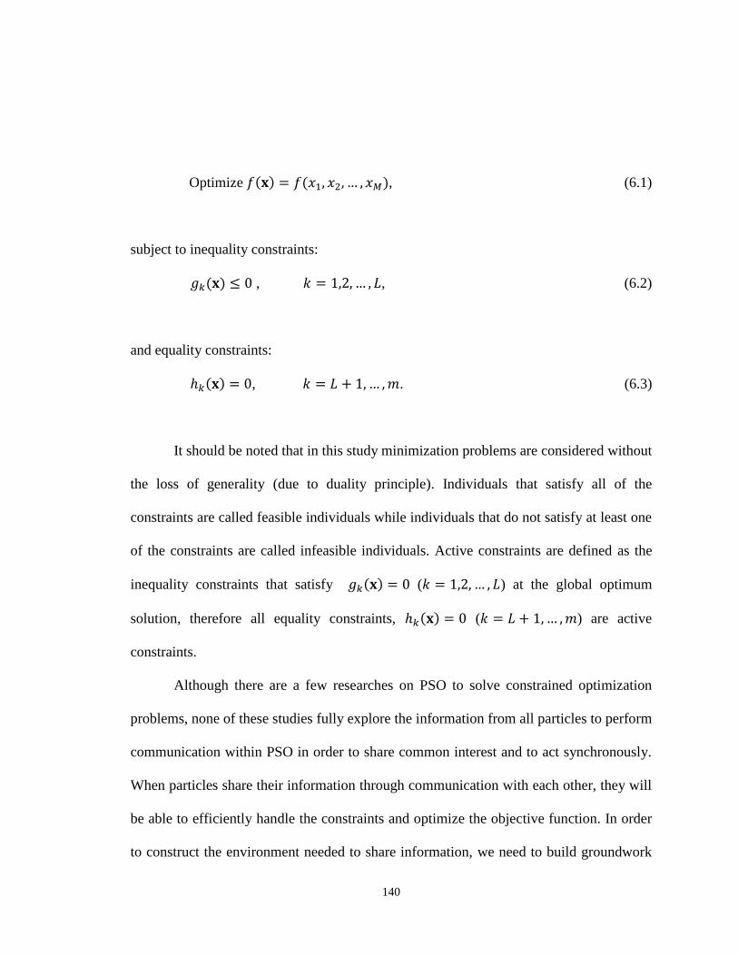
140

Optimize , (6.1)

subject to inequality constraints:

, , (6.2)

and equality constraints:

, . (6.3)

It should be noted that in this study minimization problems are considered without

the loss of generality (due to duality principle). Individuals that satisfy all of the

constraints are called feasible individuals while individuals that do not satisfy at least one

of the constraints are called infeasible individuals. Active constraints are defined as the

inequality constraints that satisfy ( ) at the global optimum

solution, therefore all equality constraints, ( ) are active

constraints.

Although there are a few researches on PSO to solve constrained optimization

problems, none of these studies fully explore the information from all particles to perform

communication within PSO in order to share common interest and to act synchronously.

When particles share their information through communication with each other, they will

be able to efficiently handle the constraints and optimize the objective function. In order

to construct the environment needed to share information, we need to build groundwork

141

to enable us to employ this information as needed. The main groundwork is the the belief

space of cultural algorithm [3, 99] which can assist the particles in an organized

informational environment to find the required information. Cultural algorithm has alone

shown its own ability to solve engineering problems [99-106, 108-112, 125, 140-142]

especially some constrained optimization ones [103-104, 111-112, 142].

From a sociological point of view, study has shown that human societies will

migrate from one place to another in order to counter their own life constraints and

limitations as well as to reach a better economical, social, or political life [8]. People

living in different societies migrate in spite of the different value systems and cultural

distinctions. Indeed the cultural belief is an important factor affecting the issues

underlying the migration phenomena [9].

On the other hand, finding the appropriate information for communication within

swarm can be computationally expensive. One computational aspect is the difficulties of

finding the appropriate information to communicate within PSO in order to be able to

simultaneously handle the constraints and optimize the objective function. Using many

concepts inspired from the cultural algorithm, such as normative knowledge, situational

knowledge, spatial knowledge, and temporal knowledge, we will be able to efficiently

and effectively organize the knowledge acquired from evolutionary process to facilitate

PSO’s updating mechanism as well as swarm communications. The inter-swarm

communication for the constrained optimization problems using PSO is an important

duty that cannot be solved unless we have access to the knowledge throughout the search

142

process given the cultural algorithm as the computational framework.

In this study, a novel computational framework based on cultural algorithm is

proposed by adopting knowledge stored in belief space in order to assist the inter-swarm

communication, to search for the leading particles in the personal level, swarm level and

global level. Every particle in CPSO will fly through a three level flight and then particles

divide into several swarms and inter-swarm communication takes place to share the

information. The remaining sections complete the presentation of this chapter as follows.

In Section 6.2, principles of cultural algorithm and related works performed in CPSO are

briefly reviewed. In Section 6.3, the proposed cultural CPSO is elaborated in details. In

Section 6.4, simulation results are evaluated on the benchmark test problems in

comparison with the state-of-the-art constraint handling models. Finally, Section 6.5

summarizes the concluding remarks and future study.


6.2.1 Related Work in Constrained PSO

Relevant works of constrained particle swarm optimization algorithms are briefly

reviewed in this subsection to motivate the proposed ideas. Particle swarm optimization

[1] has shown its promise to solve the constrained optimization problems. Hu and

Eberhart simply generated particles in PSO for the constrained optimization problems

until they are located in the feasible region and then used these particles in feasible region

for finding best personal and global particles [70]. Parsopoulos and Vrahatis used a

143

dynamic multi-stage penalty function for constraint handling [71]. The penalty function is

weighted sum of all constraints violation with each constraint having a dynamic exponent

and a multi-stage dynamic coefficient. Coath and Halgamuge presented a comparison of

two constraint handling methods based upon preserving feasible solutions [70] and

dynamic penalty function [71] to solve constrained nonlinear optimization problems

using PSO [72]. It demonstrated that the convergence rate for penalty function based PSO

was faster than that of feasible solution method.

Paquet and Engelbrecht proposed a modified PSO to solve linearly constrained

optimization problems [74]. An essential characteristic of their modified PSO is that the

movement of the particles in the vector space is mathematically guaranteed by the

velocity and position update mechanism of PSO. They proved that their modified PSO is

always assured to find at least a local optimum for linear constrained optimization

problems. Takahama and Sakai in their -constrained PSO proposed an algorithm in

which particles that satisfy the constraints move to optimize the objective function while

the particles that violate the constraints move to satisfy the constraints [75]. In order to

adaptively control the maximum velocity of the particles, particles are divided into some

groups and their movement in those groups is compared.

Krohling and Coelho adopted Gaussian distribution instead of uniform

distribution for the personal and global term random weights of the PSO mechanism to

solve constrained optimization problems formulated as min-max problems [76]. They

used two populations simultaneously; first PSO focuses on evolving the variable vector

144

while the vector of Lagrangian multiplier is kept frozen, and the second PSO is to

concentrate on evolving the Lagrangian multiplier while the first population is kept

frozen. The use of normal distribution for the stochastic parameters of the PSO seems to

provide a good compromise between the probability of having a large number of small

amplitude around the current points and small probability of having large amplitudes, that

may cause the particles to move away from the current points and escape from the local

optima.

Yang et al. [77] proposed a master-slave PSO in which master swarm is

responsible for optimizing objective function while slave swarm is focused on constraint

feasibility. Particles in the master swarm only fly toward the current better particles in the

feasible region. The slave swarm is responsible for searching feasible particles by

scouting through the infeasible region. The feasible/infeasible leaders from swarm will

then communicate to lead the other swarm. By exchanging flight information between

swarms, algorithm can explore a wider solution space.

Zheng et al. [78] adopted an approach that congregates neighboring particles in

the PSO to form multiple swarms in order to explore isolated, long and narrow feasible

space. They also applied a mutation operator with dynamic mutation rate to encourage

flight of particles to feasible region more frequently. For constraint handling a penalty

function has been adopted as to how far the infeasible particle is located from the feasible

region. Saber et al. [79] introduced a version of PSO for constrained optimization

problems. In their version of PSO, the velocity update mechanism uses a sufficient

145

number of promising vectors to reduce randomness for better convergence. The velocity

coefficient in the positional update equation is a dynamic rate depending on the error and

iteration. They also reinitialized the idle particles if there are not improvements for some

iterations.

Li et al. [80] proposed dual PSO with stochastic ranking to handle the constraints.

One regular PSO evolves simultaneously along with a genetic PSO which is a discrete

version of PSO including a reproduction operator. The better of the two positions

generated by these two PSOs is then selected as the updated position. Flores-Mendoza

and Mezura-Montes [81] used Pareto dominance concept for constraint handling on a bi-

objective space, with one objective being sum of the inequality constraint violations and

the second objective being sum of the equality constraint violations in order to promote

better approach to feasible region. They also adopted a decaying parameter control

constriction factor and global acceleration of the PSO to prevent the premature

convergence and to advance the exploration of the search space. Ting et al. [82]

introduced a hybrid heuristic consisting PSO and genetic algorithm to tackle constraint

optimization problem of load flow problems. They adopted two-point crossover,

mutation, and roulette-wheel selection from genetic algorithms along with the regular

PSO to generate the new population space. Liu et al. [83] incorporated discrete genetic

PSO with differential evolution (DE) to enhance the search process in which both genetic

PSO and DE update the position of the individual at every generation. The better position

will then be selected.

146

In [143], the constraint handling techniques are embedded into the flight

mechanism of PSO, including separate procedures to update infeasible and feasible

personal bests in order to guide the infeasible individuals towards the feasible regions

while promote search for optimal solutions. Additionally, storing infeasible

nondominated solutions along with the best feasible solutions in global best archive is to

assist the search for feasible regions and better solution. The adjustment of accelerated

constants is based on the number of feasible personal bests and the constraint violations

of personal bests and global best. Simulation study shows the proposed design is able to

obtain quality solution in a very efficient manner.

6.2.2 Related Works in Cultural Algorithm for Constrained Optimization

Originated by Reynolds [3, 99], cultural algorithm (CA) is a dual inheritance

system where information exists at two different space, population space and belief

space, and can pass along to the next generation. CA has shown its ability to solve

different types of problems among which Jin and Reynolds’s algorithm [142] enhanced

the performance of evolutionary programming as population space by adopting the belief

space in order to solve constrained optimization problems.

Researchers have identified five basic sections of knowledge stored in belief

space: situational knowledge, normative knowledge, spatial or topographical knowledge

[105], domain knowledge, and temporal or history knowledge [106]. Becerra and Coello

Coello proposed a cultured differential evolution for constrained optimization [104]. The

147

population space in their study was differential evolution (DE) while the belief space

consists of situational, topographical, normative, and history knowledge. The variation

operator in DE was influenced by the knowledge source of belief space. Yuan et al.

introduced chaotic hybrid cultural algorithm for constrained optimization in which

population space is DE and belief space includes normative and situational knowledge

[111]. They incorporated a logistic map function for better convergence of DE. Tang and

Li proposed a cultured genetic algorithm for constrained optimization problems by

introducing a triple space cultural algorithm [112]. The triple space includes belief space,

population space in addition to an anti-culture population consisting individuals

disobeying the guidance of the belief space and going away from the belief space guided

individuals. The effect of disobeying enhanced by some mutation operations appreciably

makes the algorithm faster and less risky for premature convergence, by awarding the

most successful individuals and punishing the most unsuccessful population.

6.3 Cultural Constrained Optimization Using Multiple-Swarm PSO

The pseudocode of the proposed design is shown in Figure 6.1 and a block

diagram depicting the operation of the proposed algorithm is also shown in Figure 6.2.

The population space (PSO) will be initialized and then divided into several swarms

based upon the proximity of the particles. The correspondent belief space (BLF) will then

be initialized. We then evaluate population space using the fitness values. Acceptance

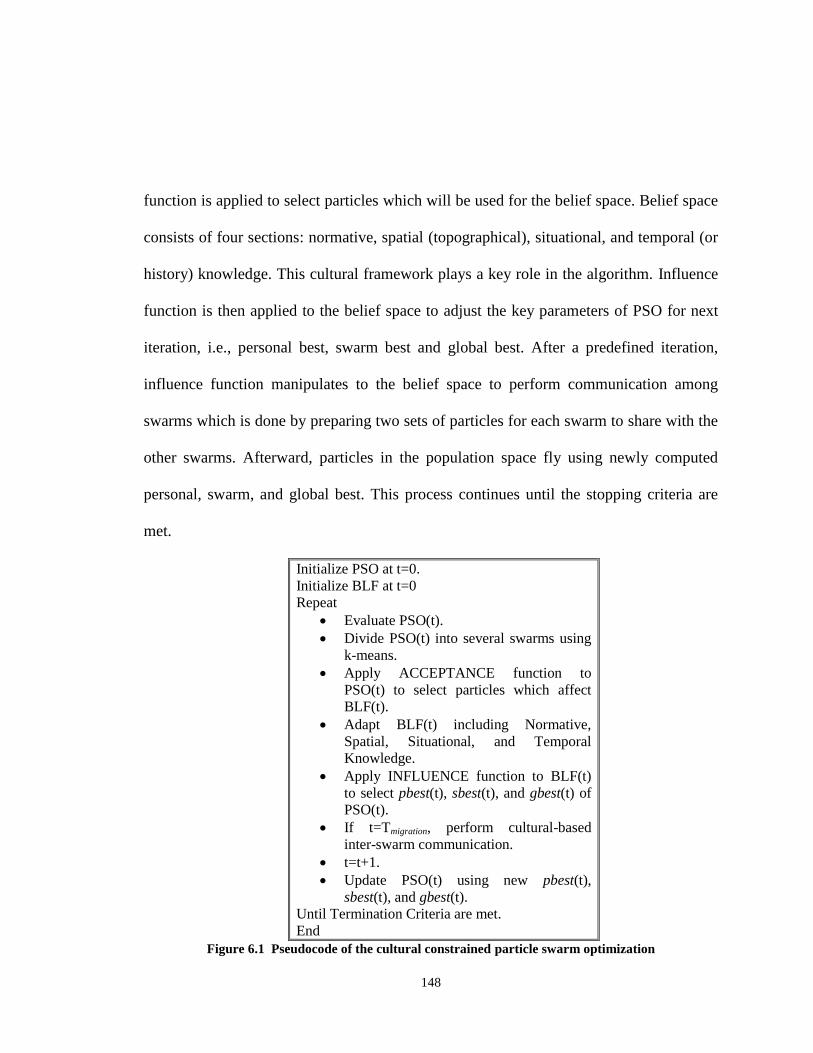
148

function is applied to select particles which will be used for the belief space. Belief space

consists of four sections: normative, spatial (topographical), situational, and temporal (or

history) knowledge. This cultural framework plays a key role in the algorithm. Influence

function is then applied to the belief space to adjust the key parameters of PSO for next

iteration, i.e., personal best, swarm best and global best. After a predefined iteration,

influence function manipulates to the belief space to perform communication among

swarms which is done by preparing two sets of particles for each swarm to share with the

other swarms. Afterward, particles in the population space fly using newly computed

personal, swarm, and global best. This process continues until the stopping criteria are

met.

Initialize PSO at t=0. Initialize BLF at t=0 Repeat

Evaluate PSO(t).

Divide PSO(t) into several swarms using

k-means.

Apply ACCEPTANCE function to

PSO(t) to select particles which affect

BLF(t).

Adapt BLF(t) including Normative,

Spatial, Situational, and Temporal

Knowledge.

Apply INFLUENCE function to BLF(t)

to select pbest(t), sbest(t), and gbest(t) of

PSO(t).

If t=Tmigration, perform cultural-based

inter-swarm communication.

t=t+1.

Update PSO(t) using new pbest(t),

sbest(t), and gbest(t).

Until Termination Criteria are met. End

Figure 6.1 Pseudocode of the cultural constrained particle swarm optimization

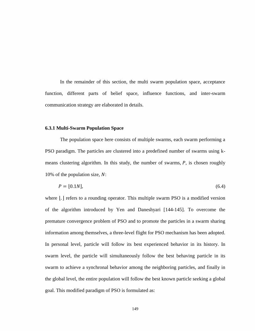
149

In the remainder of this section, the multi swarm population space, acceptance

function, different parts of belief space, influence functions, and inter-swarm

communication strategy are elaborated in details.

6.3.1 Multi-Swarm Population Space

The population space here consists of multiple swarms, each swarm performing a

PSO paradigm. The particles are clustered into a predefined number of swarms using k-

means clustering algorithm. In this study, the number of swarms, , is chosen roughly

10% of the population size, :

(6.4)

where refers to a rounding operator. This multiple swarm PSO is a modified version

of the algorithm introduced by Yen and Daneshyari [144-145]. To overcome the

premature convergence problem of PSO and to promote the particles in a swarm sharing

information among themselves, a three-level flight for PSO mechanism has been adopted.

In personal level, particle will follow its best experienced behavior in its history. In

swarm level, the particle will simultaneously follow the best behaving particle in its

swarm to achieve a synchronal behavior among the neighboring particles, and finally in

the global level, the entire population will follow the best known particle seeking a global

goal. This modified paradigm of PSO is formulated as:

150

,

, (6.5)

where is the -th dimension of velocity of the -th particle at time ,

is the

-th dimension of position of the -th particle at time , is the -th dimension

of best past position of the -th particle at time , is defined as the -th

dimension of best particle from swarm in which particle belongs. is the -

th dimension of the best particle of population at time . , and are uniformly

generated random numbers in the range of , , and are constant parameters

representing the weights for personal, swarm, and global behavior and is the

momentum for previous velocity.


The belief space should be affected by a selection of best individuals. Therefore

all particles located in the feasible space, along with % of the infeasible particles that

have the least violation of constraints are selected, where is a predefined value. This

allows infeasible individuals with minimum constraint violations to portray feasibility

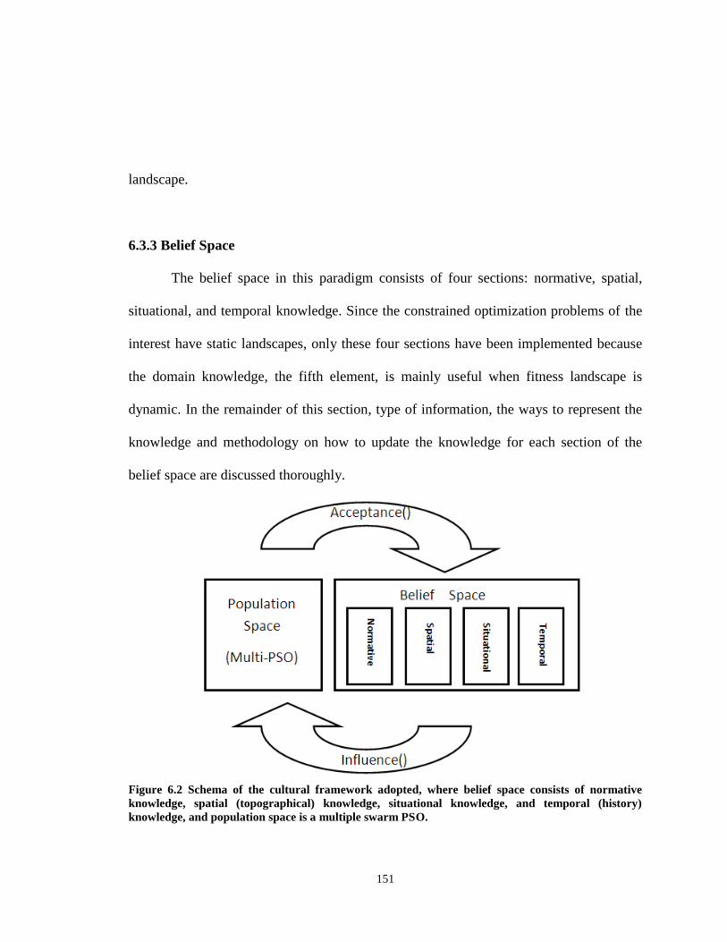
151

landscape.

6.3.3 Belief Space

The belief space in this paradigm consists of four sections: normative, spatial,

situational, and temporal knowledge. Since the constrained optimization problems of the

interest have static landscapes, only these four sections have been implemented because

the domain knowledge, the fifth element, is mainly useful when fitness landscape is

dynamic. In the remainder of this section, type of information, the ways to represent the

knowledge and methodology on how to update the knowledge for each section of the

belief space are discussed thoroughly.

Figure 6.2 Schema of the cultural framework adopted, where belief space consists of normative

knowledge, spatial (topographical) knowledge, situational knowledge, and temporal (history)

knowledge, and population space is a multiple swarm PSO.

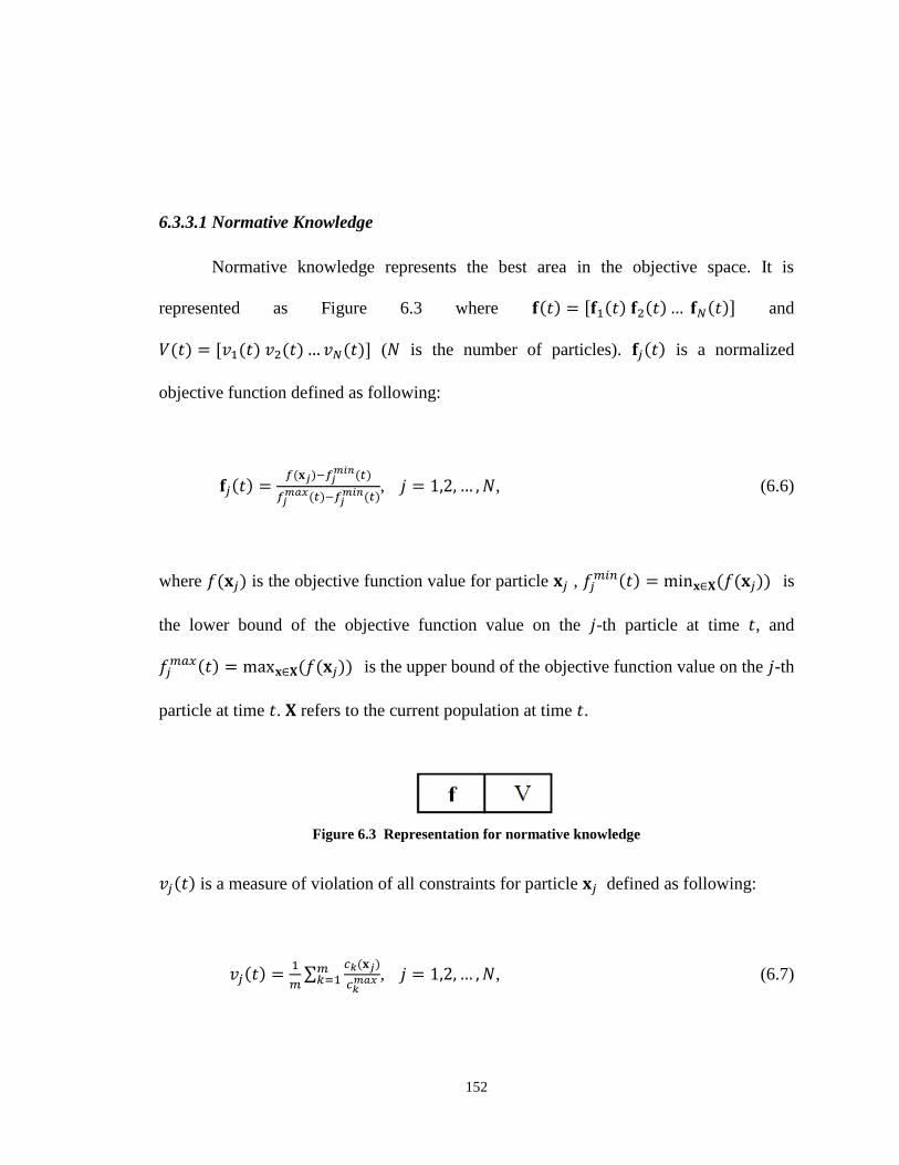
152


Normative knowledge represents the best area in the objective space. It is

represented as Figure 6.3 where and

( is the number of particles). is a normalized

objective function defined as following:

, , (6.6)

where is the objective function value for particle , is

the lower bound of the objective function value on the -th particle at time , and

is the upper bound of the objective function value on the -th

particle at time . refers to the current population at time .

Figure 6.3 Representation for normative knowledge

is a measure of violation of all constraints for particle defined as following:

, , (6.7)

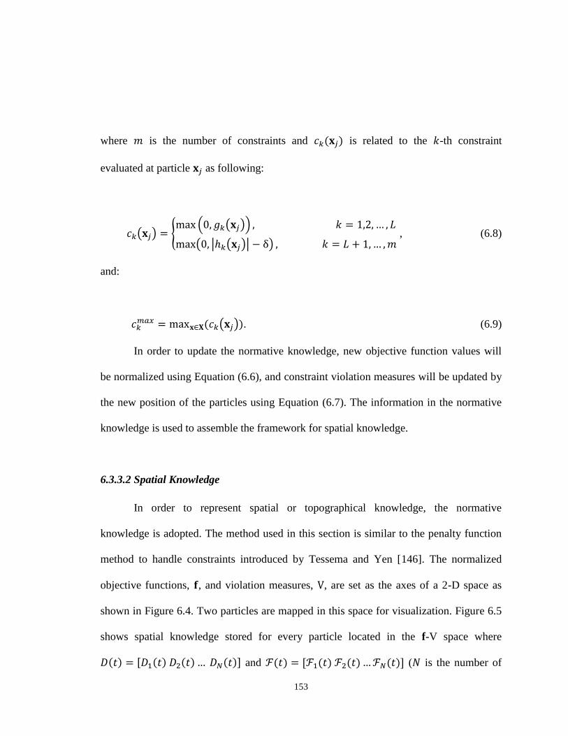
153

where is the number of constraints and is related to the -th constraint

evaluated at particle as following:

, (6.8)

and:

. (6.9)

In order to update the normative knowledge, new objective function values will

be normalized using Equation (6.6), and constraint violation measures will be updated by

the new position of the particles using Equation (6.7). The information in the normative

knowledge is used to assemble the framework for spatial knowledge.

6.3.3.2 Spatial Knowledge

In order to represent spatial or topographical knowledge, the normative

knowledge is adopted. The method used in this section is similar to the penalty function

method to handle constraints introduced by Tessema and Yen [146]. The normalized

objective functions, , and violation measures, , are set as the axes of a 2-D space as

shown in Figure 6.4. Two particles are mapped in this space for visualization. Figure 6.5

shows spatial knowledge stored for every particle located in the f-V space where

and ( is the number of

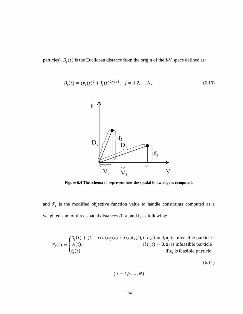
154

particles). is the Euclidean distance from the origin of the f-V space defined as:

, , (6.10)

Figure 6.4 The schema to represent how the spatial knowledge is computed.

and is the modified objective function value to handle constraints computed as a

weighted sum of three spatial distances , , and , as following:

,

(6.11)

155

where is the ratio of number of feasible particles over the population size, and

are defined in Equations (6.6) and (6.7), respectively. If , then

will be more important than in Equation (6.11), consequently in

schema shown in Figure 6.4, which means particle 2 outperforms particle 1 for a

minimization problem. But when , then will be more important than

in Equation (6.11), consequently in schema shown in Figure 6.4,

which in turn means particle 1 outperforms particle 2.

Figure 6.5 Representation of spatial knowledge for each particle

At every iteration, the spatial knowledge will be updated. To do so, updated

normative knowledge will be used to rebuild the spatial distance for every particle using

Equations (6.10) and (6.11). Spatial knowledge will be used later to find the global best

particle of population space and to build a communication strategy among swarms.


This part of belief space is used to keep the good exemplar particles for each

swarm. Its representation is shown in Figure 6.6. ( ) where is the

number of swarms defined in Equation (6.4), the best particle in the -th swarm based

156

upon information received from the spatial knowledge in accordance with both objective

function value and constraints violation. Assume that at an arbitrary iteration the -th

swarm consists particles as and that

is a set

consisting the modified objective values extracted from the spatial knowledge

corresponding to , respectively. Then is defined such that:

, , (6.12)

Figure 6.6 Representation for situational knowledge

where is the modified objective function value for the particle . In order

to update the situational knowledge, the updated position of the particles will be used to

evaluate Equations (6.6) to (6.11) to compute updated modified objective function values,

and then the particle corresponding to the least value in each swarm will be stored in

situational knowledge. The situational knowledge will be used later to compute the

swarm best particles and to facilitate the communication among swarms.

6.3.3.4 Temporal Knowledge

This part of belief space is used to keep the history of the individual’s behavior.

Its representation is shown in Figure 6.7 where and

157

( is the number of particles). is a set of past

temporal pattern of the -th particle which are collected at every time step from part of

the spatial knowledge, , and is defined as following:

Figure 6.7 Representation for temporal knowledge

, , (6.13)

where and are the modified objective function values defined in

Equation (6.11) for the time steps , respectively. is the set of all past

positions of the -th particle in the whole population defined as

, . The temporal knowledge will be updated

at every iteration. To do so, the updated spatial knowledge, the updated position of the

particle, and previously stored temporal knowledge will be adopted as following:

,

, (6.14)

The temporal knowledge will later be used to compute the personal best for every

particle in the population space.

158


After belief space is updated, the correspondent knowledge should be used to

influence the flight of particles in PSO. We propose to use the knowledge in belief space

to select the personal best, swarm best, and global best for the PSO flight mechanism.

Furthermore, we propose to adopt the information in the belief space to perform a

communication strategy among swarms.

6.3.4.1 Selection

In order to select the personal best, we exploit information in the temporal

knowledge section of the belief space. The best behaving particle’s past history should be

selected as following:

, (6.15)

where is the set of all past positions of the -th particle,

and is the corresponding modified objective values for

the past history of the -th particle both extracted from the temporal knowledge section of

the belief space.

6.3.4.2 Selection

159

In order to select the swarm best particle, the situational knowledge is adopted.

The information stored in the situational knowledge section of the belief space is simply

copied into swarm best particles:

, , (6.16)

where is the number of swarms and is the representation of the situational

knowledge in the belief space.

6.3.4.3 Selection

The spatial knowledge stored in the belief space is used to compute gbest(t) at

each iteration. The global best particle is found as following:

, (6.17)

where , is the entire population of particles at time , and

is a set consisting of the modified objective function

values for all particles at time .

6.3.4.4 Inter-Swarm Communication Strategy

160

After some predefined iterations, , the swarms will perform information

exchange. Each swarm prepares a list of sending particles to be sent to the next swarm,

and also assembles a list of replacement particles to be replaced by particles coming from

other swarms. This communication strategy is a modified version of the algorithm

adopted in [145]. We use the information stored in the belief space to perform

communication among swarms. To do so, each swarm prepares two list of particles

and , where is the fixed number of swarms defined in Equation (6.4) .

is a list of particles in the -th swarm to be sent to the next swarm and is a list of

particles in the -th swarm to be replaced by particles coming from another swarm. The

inter-swarm communication strategy is based upon the particles’ locations in the swarm

and their modified objective value which is stored in the belief space. The sending list for

the swarm is prepared in the following order:

(1) The highest priority in the selection of particles is given to a particle that has

the least average Hamming distance from others. This particle is considered as the

representative of the swarm.

(2) The second priority is given to the closest particles to the representative particle in

the -th swarm whose modified objective value stored in the spatial knowledge of the

belief space is greater than that of the representative. is defined as [144]:

, (6.18)

161

where , rate of information exchange among swarms, is a predefined value between 0

and 1, is the population of the -th swarm.

(3) The third priority is given to the closest particles to the representative particle

whose modified objective value extracted from the belief space is less than that of the

representative.

(4) The fourth and last priority is given to the best performing particle in the

swarm.

Note that depending on the predefined fixed value for allowable number of the

sending list, , the sending list will be filled in each swarm using the above-

mentioned priorities.

There will also be a replacement list that each swarm prepares, based upon the

similar positional information of particles in the swarm. When swarms are approaching

local optima, many particles’ locations are the same. Each swarm will remove this excess

information through its replacement list. The replacement list in each swarm is assembled

in the following order:

(1) The first priority is given to the particles with identical decision space

information in the order of their modified objective values extracted from the belief

space, with the least modified objective values being replaced first.

(2) The second and last priority is given to the particles with the lowest modified

objective values if all particles of the first priority have already been placed in the

replacement list.

162

This information exchange among swarms happens in a ring sequential order

between each pair of swarms. Each swarm accepts the sending list from other swarm and

will replace it with its own replacement list.

6.4 Comparative Study

In this section, the performance of the cultural CPSO is evaluated against those of

the selected state-of-the-art constrained optimization heuristics.

6.4.1 Parameter Settings

The parameters of the cultural CPSO are set as shown in Table 6.1. The tolerance

for equality constraints in Equation (6.8), , is set as 0.0001. In the flight mechanism, the

momentum, , is randomly selected from the uniform distribution of (0.5, 1), the

personal, swarm and global acceleration, , and are all selected as 1.5.

Table 6.1 Parameter settings for cultural CPSO

Tolerance for equality constraints in Equation (6.8) 0.0001

Momentum in Equation (6.5)

Personal acceleration in Equation (6.5) 1.5

Swarm acceleration in Equation (6.5) 1.5

Global acceleration in Equation (6.5) 1.5

N Population size 100

Rate of information exchange in Equation (6.18) 30%

Allowable number of migrating particles

nnnnnnnnnnnnnnnnnnnnnnnnnnnnnnnnnnnnnnnnnn

nnnnnnnnnnnnnnnnnnnnnnnnnnnnnnnnnnnnn=0.05

N

5

163

The population size is fixed at 100 particles. The maximum velocity for the

particles in specific dimension, , is set at half of the range of the particle’s position in

that dimension:

. (6.19)

The rate for information exchange among swarms affects how much swarms

communicate with each other. The higher rate corresponds to more communication and

better overall performance of the algorithm, but it does incur higher computational

complexity, while a lower rate imposes less computational complexity and relatively

poorer performance. The heuristic choice is set at 30%. The allowable number of

migrating particles among swarms is set as 5% of the population size, which is

.

6.4.2 Benchmark Test Functions

The proposed cultural CPSO has been tested on 24 benchmark functions [147] to

verify its performance. The characteristics on these test functions are summarized in

Table 6.2. These problems include various types of objective functions such as linear,

nonlinear, quadratic, cubic, and polynomial. These benchmark problems vary in the

number of decision variables, , between 2 and 24, and number of constraints, between 1

and 38. In this table, is the estimated ratio of the feasible region over the search space

which varies as low as 0.0000% to as high as 99.9971%. The numbers of different types

of constraints are also shown for each test function: the number of linear inequality (LI),

164

the number of nonlinear inequality (NI), the number of linear equality (LE) and the

number of nonlinear equality (NE). In this table, is the number of active constraints at

the known optimal solution, , and is the objective function of the known optimal

solution [147]. The detailed formulation of these benchmark test functions are presented

in Appendix B for reference.

6.4.3 Simulation Results

The experiments reported in this study are performed on a computer with 1.66

GHz Duel-Core Processor and 1GB RAM operating on a Windows XP Professional. The

programs are written in Matlab. Extensive experiments have been performed on all 24

benchmark test functions based upon comparison methods suggested in [147] which are

explicitly followed by researchers in the field in order to have meaningful comparison.

For three different functions evaluations (FEs) of 5,000, 50,000, and 500,000, the

objective function error values, are found, while is the best known

solution [147] presented in the rightmost column in Table 6.2. Notice when

, the final error is considered as zero. For each benchmark test problem,

a total of 25 independent runs are performed.

The statistical measures including the best, median, worst, mean and standard

deviations are then computed. These results are tabulated in Tables 6.3 to 6.6. For the

best, median and worst solutions, the number of constraints that can not satisfy feasibility

condition is found and shown as an integer inside parenthesis after the best, median, and

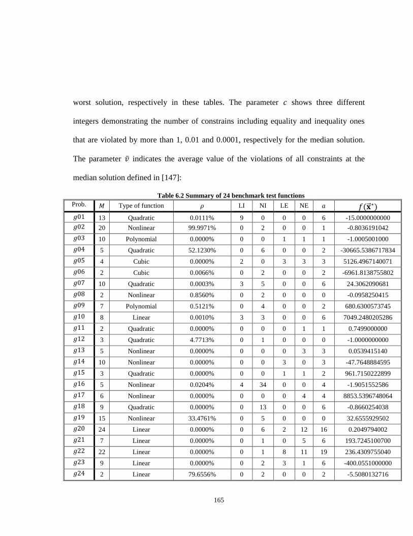
165

worst solution, respectively in these tables. The parameter shows three different

integers demonstrating the number of constrains including equality and inequality ones

that are violated by more than 1, 0.01 and 0.0001, respectively for the median solution.

The parameter indicates the average value of the violations of all constraints at the

median solution defined in [147]:

Table 6.2 Summary of 24 benchmark test functions

Prob. Type of function LI NI LE NE

13 Quadratic 0.0111% 9 0 0 0 6 -15.0000000000

20 Nonlinear 99.9971% 0 2 0 0 1 -0.8036191042

10 Polynomial 0.0000% 0 0 1 1 1 -1.0005001000

5 Quadratic 52.1230% 0 6 0 0 2 -30665.5386717834

4 Cubic 0.0000% 2 0 3 3 3 5126.4967140071

2 Cubic 0.0066% 0 2 0 0 2 -6961.8138755802

10 Quadratic 0.0003% 3 5 0 0 6 24.3062090681

2 Nonlinear 0.8560% 0 2 0 0 0 -0.0958250415

7 Polynomial 0.5121% 0 4 0 0 2 680.6300573745

8 Linear 0.0010% 3 3 0 0 6 7049.2480205286

2 Quadratic 0.0000% 0 0 0 1 1 0.7499000000

3 Quadratic 4.7713% 0 1 0 0 0 -1.0000000000

5 Nonlinear 0.0000% 0 0 0 3 3 0.0539415140

10 Nonlinear 0.0000% 0 0 3 0 3 -47.7648884595

3 Quadratic 0.0000% 0 0 1 1 2 961.7150222899

5 Nonlinear 0.0204% 4 34 0 0 4 -1.9051552586

6 Nonlinear 0.0000% 0 0 0 4 4 8853.5396748064

9 Quadratic 0.0000% 0 13 0 0 6 -0.8660254038

15 Nonlinear 33.4761% 0 5 0 0 0 32.6555929502

24 Linear 0.0000% 0 6 2 12 16 0.2049794002

7 Linear 0.0000% 0 1 0 5 6 193.7245100700

22 Linear 0.0000% 0 1 8 11 19 236.4309755040

9 Linear 0.0000% 0 2 3 1 6 -400.0551000000

2 Linear 79.6556% 0 2 0 0 2 -5.5080132716

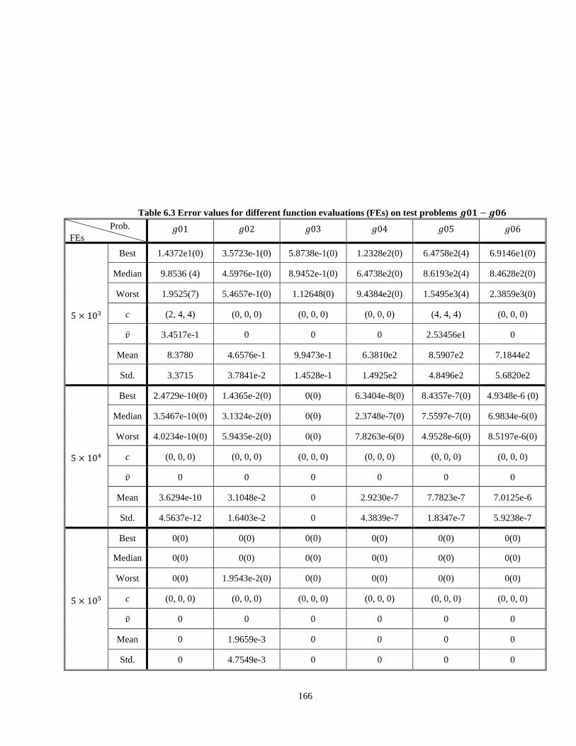
166

Table 6.3 Error values for different function evaluations (FEs) on test problems

Prob.

FEs

Best 1.4372e1(0) 3.5723e-1(0) 5.8738e-1(0) 1.2328e2(0) 6.4758e2(4) 6.9146e1(0)

Median 9.8536 (4) 4.5976e-1(0) 8.9452e-1(0) 6.4738e2(0) 8.6193e2(4) 8.4628e2(0)

Worst 1.9525(7) 5.4657e-1(0) 1.12648(0) 9.4384e2(0) 1.5495e3(4) 2.3859e3(0)

c (2, 4, 4) (0, 0, 0)

0000

(0, 0, 0) (0, 0, 0) (4, 4, 4) (0, 0, 0)

3.4517e-1 0 0 0 2.53456e1 0

Mean 8.3780 4.6576e-1 9.9473e-1 6.3810e2 8.5907e2 7.1844e2

Std. 3.3715 3.7841e-2 1.4528e-1 1.4925e2 4.8496e2 5.6820e2

Best 2.4729e-10(0) 1.4365e-2(0) 0(0) 6.3404e-8(0) 8.4357e-7(0) 4.9348e-6 (0)

Median 3.5467e-10(0) 3.1324e-2(0) 0(0) 2.3748e-7(0)

7.5597e-7(0) 6.9834e-6(0)

Worst 4.0234e-10(0) 5.9435e-2(0) 0(0) 7.8263e-6(0) 4.9528e-6(0) 8.5197e-6(0)

c (0, 0, 0) (0, 0, 0) (0, 0, 0) (0, 0, 0) (0, 0, 0) (0, 0, 0)

0 0 0 0 0 0

Mean 3.6294e-10 3.1048e-2 0 2.9230e-7 7.7823e-7 7.0125e-6

Std. 4.5637e-12 1.6403e-2 0 4.3839e-7 1.8347e-7 5.9238e-7

Best 0(0) 0(0) 0(0) 0(0) 0(0) 0(0)

Median 0(0) 0(0) 0(0) 0(0) 0(0) 0(0)

Worst 0(0) 1.9543e-2(0) 0(0) 0(0) 0(0) 0(0)

c (0, 0, 0) (0, 0, 0) (0, 0, 0) (0, 0, 0) (0, 0, 0) (0, 0, 0)

0 0 0 0 0 0

Mean 0 1.9659e-3 0 0 0 0

Std. 0 4.7549e-3 0 0 0 0

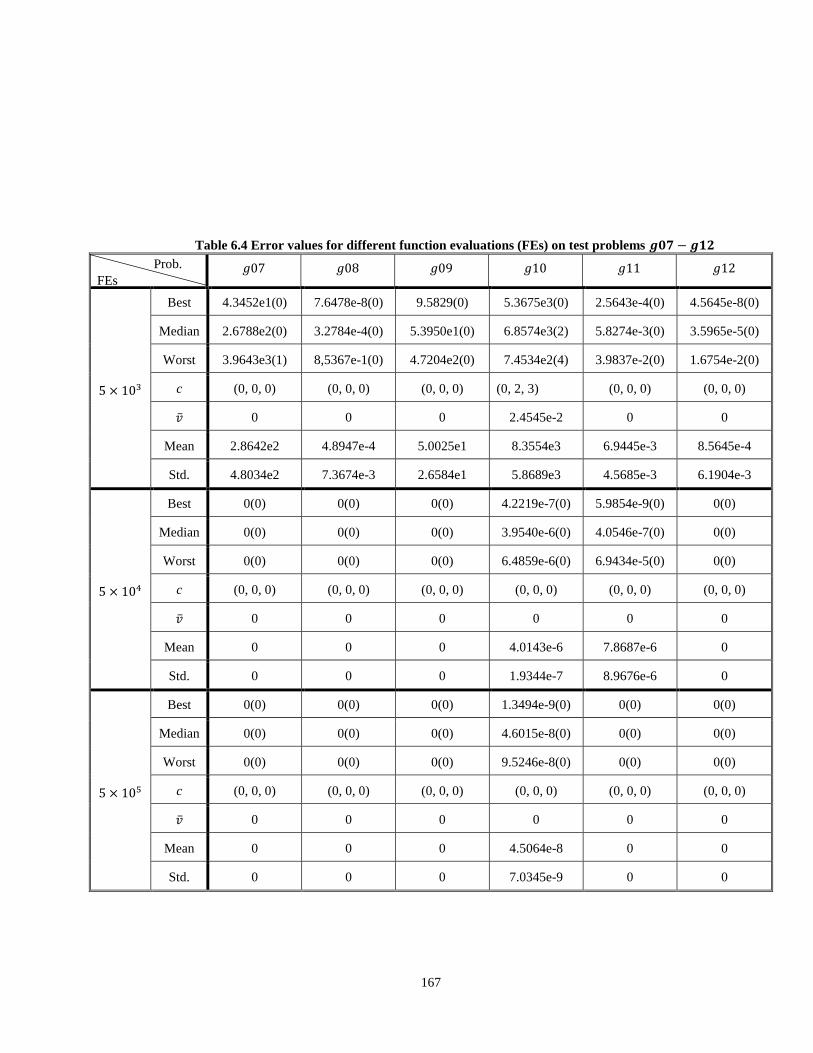
167


Prob.

FEs

Best 4.3452e1(0) 7.6478e-8(0) 9.5829(0) 5.3675e3(0) 2.5643e-4(0) 4.5645e-8(0)

Median 2.6788e2(0) 3.2784e-4(0) 5.3950e1(0) 6.8574e3(2) 5.8274e-3(0) 3.5965e-5(0)

Worst 3.9643e3(1) 8,5367e-1(0) 4.7204e2(0) 7.4534e2(4) 3.9837e-2(0) 1.6754e-2(0)

c (0, 0, 0) (0, 0, 0) (0, 0, 0) (0, 2, 3) (0, 0, 0) (0, 0, 0)

0 0 0 2.4545e-2 0 0

Mean 2.8642e2 4.8947e-4 5.0025e1 8.3554e3 6.9445e-3 8.5645e-4

Std. 4.8034e2 7.3674e-3 2.6584e1 5.8689e3 4.5685e-3 6.1904e-3

Best 0(0) 0(0) 0(0) 4.2219e-7(0) 5.9854e-9(0) 0(0)

Median 0(0) 0(0) 0(0) 3.9540e-6(0) 4.0546e-7(0) 0(0)

Worst 0(0) 0(0) 0(0) 6.4859e-6(0) 6.9434e-5(0) 0(0)

c (0, 0, 0) (0, 0, 0) (0, 0, 0) (0, 0, 0) (0, 0, 0) (0, 0, 0)

0 0 0 0 0 0

Mean 0 0 0 4.0143e-6 7.8687e-6 0

Std. 0 0 0 1.9344e-7 8.9676e-6 0

Best 0(0) 0(0) 0(0) 1.3494e-9(0) 0(0) 0(0)

Median 0(0) 0(0) 0(0) 4.6015e-8(0) 0(0) 0(0)

Worst 0(0) 0(0) 0(0) 9.5246e-8(0) 0(0) 0(0)

c (0, 0, 0) (0, 0, 0) (0, 0, 0) (0, 0, 0) (0, 0, 0) (0, 0, 0)

0 0 0 0 0 0

Mean 0 0 0 4.5064e-8 0 0

Std. 0 0 0 7.0345e-9 0 0

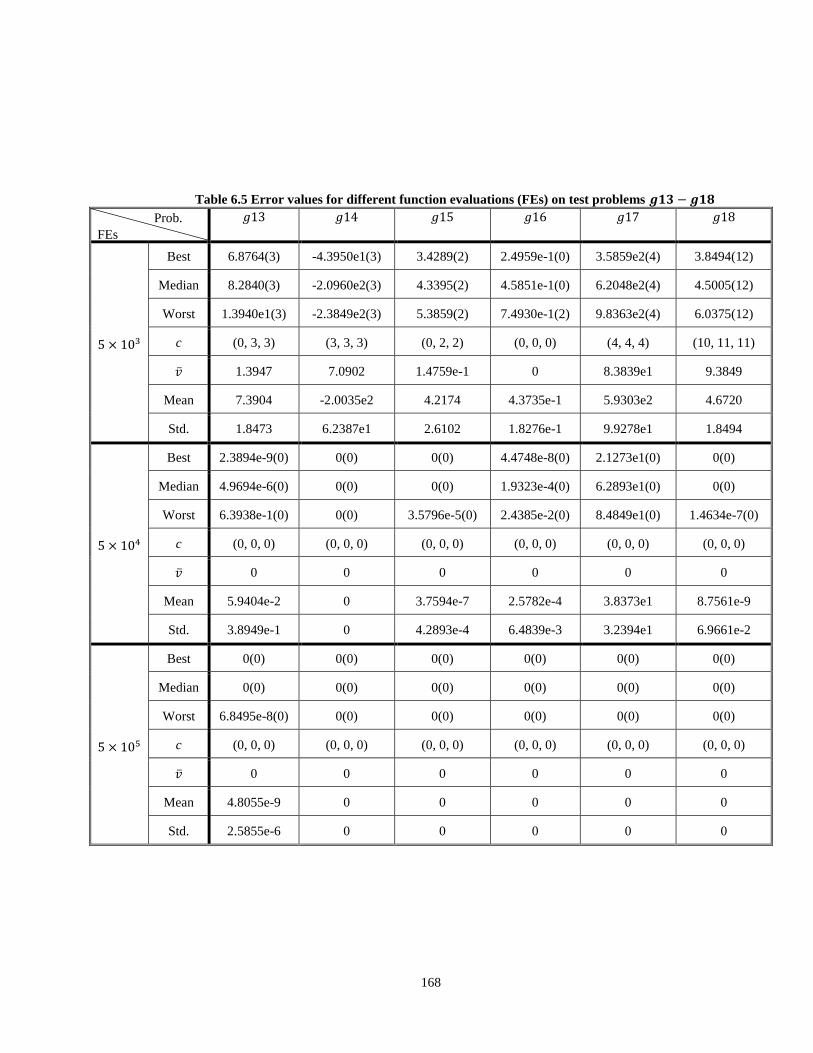
168


Prob.

FEs

Best 6.8764(3) -4.3950e1(3) 3.4289(2) 2.4959e-1(0) 3.5859e2(4) 3.8494(12)

Median 8.2840(3) -2.0960e2(3) 4.3395(2) 4.5851e-1(0) 6.2048e2(4) 4.5005(12)

Worst 1.3940e1(3) -2.3849e2(3) 5.3859(2) 7.4930e-1(2) 9.8363e2(4) 6.0375(12)

c (0, 3, 3) (3, 3, 3) (0, 2, 2) (0, 0, 0) (4, 4, 4) (10, 11, 11)

1.3947 7.0902 1.4759e-1 0 8.3839e1 9.3849

Mean 7.3904 -2.0035e2 4.2174 4.3735e-1 5.9303e2 4.6720

Std. 1.8473 6.2387e1 2.6102 1.8276e-1 9.9278e1 1.8494

Best 2.3894e-9(0) 0(0) 0(0) 4.4748e-8(0) 2.1273e1(0) 0(0)

Median 4.9694e-6(0) 0(0) 0(0) 1.9323e-4(0) 6.2893e1(0) 0(0)

Worst 6.3938e-1(0) 0(0) 3.5796e-5(0) 2.4385e-2(0) 8.4849e1(0) 1.4634e-7(0)

c (0, 0, 0) (0, 0, 0) (0, 0, 0) (0, 0, 0) (0, 0, 0) (0, 0, 0)

0 0 0 0 0 0

Mean 5.9404e-2 0 3.7594e-7 2.5782e-4 3.8373e1 8.7561e-9

Std. 3.8949e-1 0 4.2893e-4 6.4839e-3 3.2394e1 6.9661e-2

Best 0(0) 0(0) 0(0) 0(0) 0(0) 0(0)

Median 0(0) 0(0) 0(0) 0(0) 0(0) 0(0)

Worst 6.8495e-8(0) 0(0) 0(0) 0(0) 0(0) 0(0)

c (0, 0, 0) (0, 0, 0) (0, 0, 0) (0, 0, 0) (0, 0, 0) (0, 0, 0)

0 0 0 0 0 0

Mean 4.8055e-9 0 0 0 0 0

Std. 2.5855e-6 0 0 0 0 0

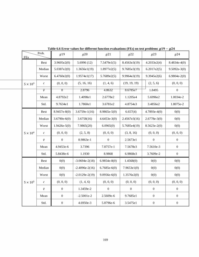
169


Prob.

FEs

Best 3.9605e2(0) 5.6996 (12) 7.5479e1(5) 8.4563e3(19) 4.2033e2(4) 8.4834e-4(0)

Median 5.0387e2(0) 1.3656e1(19) 1.8977e2(5) 9.7685e3(19) 6.2017e2(5) 9.5092e-3(0)

Worst 6.4760e2(0) 1.9574e1(17) 5.7689e2(5) 9.9964e3(19) 9.3945e2(6) 6.9804e-2(0)

c (0, 0, 0)

(5, 16, 16) (1, 4, 6) (19, 19, 19) (2, 5, 6) (0, 0, 0)

0 2.8796 4.8632 8.6785e7 1.8495 0

Mean 4.8792e2 1.4098e1 2.6778e2 1.1205e4 5.6996e2 1.0034e-2

Std. 9.7634e1 1.7860e1 3.6781e2 4.8754e3 3.4856e2 1.8075e-2

Best 8.9457e-8(0) 3.6759e-1(16) 8.9865e-5(0) 6.657(4) 4.7893e-4(0) 0(0)

Median 3.6790e-6(0) 3.6758(16) 4.6453e-3(0) 2.4567e3(16) 2.6778e-3(0) 0(0)

Worst 1.9426e-5(0) 7.9865(20) 6.0965(0) 5.7685e4(19) 8.5623e-2(0) 0(0)

c (0, 0, 0) (2, 5, 8) (0, 0, 0) (3, 8, 16) (0, 0, 0) (0, 0, 0)

0 8.9863e-1 0 2.5673e1 0 0

Mean 4.9453e-6 3.7396 7.8757e-1 7.5678e3 7.5610e-3 0

Std. 5.8438e-6 1.1930 8.9868 6.9868e3 3.7609e-2 0

Best 0(0) -3.0694e-2(18) 6.9854e-8(0) 1.4568(0) 0(0) 0(0)

Median 0(0) -2.4096e-2(16) 6.7685e-6(0) 7.9653e1(0) 0(0) 0(0)

Worst 0(0) -2.0129e-2(19) 9.0956e-6(0) 1.3576e2(0) 0(0) 0(0)

c (0, 0, 0) (1, 4, 6) (0, 0, 0) (0, 0, 0) (0, 0, 0) (0, 0, 0)

0 1.3459e-2 0 0 0 0

Mean 0 -2.5001e-2 2.5609e-6 9.7685e1 0 0

Std. 0 4.6950e-3 5.8796e-6 3.5475e1 0 0

170

, (6.20)

where:

, , (6.21)

and:

, , (6.22)

For each independent run, the number of function evaluations to locate a solution

satisfying is recorded. For each benchmark function, statistical

measures of these 25 runs including the best, median, worst, mean, and standard

deviations are then computed. These results are shown in Table 6.7. In the same table,

Feasible Rate, Success Rate and Success Performance are also calculated for each test

function. Feasible Rate is a ratio of feasible runs over total runs, where feasible run is

defined as a run with maximum function evaluation of 500,000 during which at least one

feasible solution is found. Successful Rate is a ratio of successful runs over the total runs,

where successful run is defined as a run during which the algorithm finds a feasible

solution, , satisfying . Success Performance is defined as [147]:

(6.23)

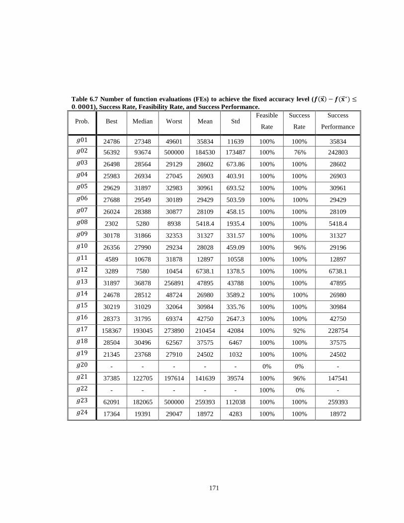
171

Table 6.7 Number of function evaluations (FEs) to achieve the fixed accuracy level ( ), Success Rate, Feasibility Rate, and Success Performance.

Prob. Best Median Worst Mean Std Feasible

Rate

Success

Rate

Success

Performance

24786 27348 49601 35834 11639 100% 100% 35834

56392 93674 500000 184530 173487 100% 76% 242803

26498 28564 29129 28602 673.86 100% 100% 28602

25983 26934 27045 26903 403.91 100% 100% 26903

29629 31897 32983 30961 693.52 100% 100% 30961

27688 29549 30189 29429 503.59 100% 100% 29429

26024 28388 30877 28109 458.15 100% 100% 28109

2302 5280 8938 5418.4 1935.4 100% 100% 5418.4

30178 31866 32353 31327 331.57 100% 100% 31327

26356 27990 29234 28028 459.09 100% 96% 29196

4589 10678 31878 12897 10558 100% 100% 12897

3289 7580 10454 6738.1 1378.5 100% 100% 6738.1

31897 36878 256891 47895 43788 100% 100% 47895

24678 28512 48724 26980 3589.2 100% 100% 26980

30219 31029 32064 30984 335.76 100% 100% 30984

28373 31795 69374 42750 2647.3 100% 100% 42750

158367 193045 273890 210454 42084 100% 92% 228754

28504 30496 62567 37575 6467 100% 100% 37575

21345 23768 27910 24502 1032 100% 100% 24502

- - - - - 0% 0% -

37385 122705 197614 141639 39574 100% 96% 147541

- - - - - 100% 0% -

62091 182065 500000 259393 112038 100% 100% 259393

17364 19391 29047 18972 4283 100% 100% 18972

172

These tables show that feasible solutions can be reliably found within the

maximum FEs for all benchmark problems except for function . The final solutions

of all benchmark problems can be identified with an error of less than 0.0001 from the

optimal solution within the maximum FEs except for functions and . Most

benchmark functions find the optimal solution with the error of less than 0.0001 before

50,000 FEs except for functions , , , and . It can also be observed

that cultural CPSO has 100% feasible rate for all benchmark problems except function

, and 100% success rate for all benchmark problems except for functions , ,

, and . However it should be noted that for functions , and the

success rate is fairly high at 96%, 92% and 96%, respectively. Summary of statistical

results for the best, median, mean, worst, and standard deviation obtained by cultural

CPSO over 25 independent runs are summarized in Table 6.8. As it can be seen in this

table, except for function , feasible solutions have been found for all other

benchmark problems.

6.4.4 Convergence Graphs

For the median run for each test function with the function evaluations (FEs) of

500,000, two semi-log graphs are plotted for each test function. The first graph is

vs. FEs, while is given in the rightmost column of Table 6.2,

and is the objective value for the best solution at the specific FE. The second graph

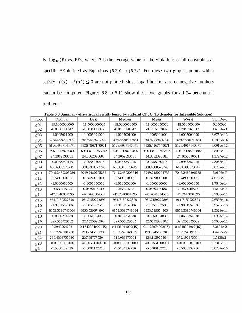
173

is vs. FEs, where is the average value of the violations of all constraints at

specific FE defined as Equations (6.20) to (6.22). For these two graphs, points which

satisfy are not plotted, since logarithm for zero or negative numbers

cannot be computed. Figures 6.8 to 6.11 show these two graphs for all 24 benchmark

problems.

Table 6.8 Summary of statistical results found by cultural CPSO (IS denotes for Infeasible Solution)

Prob. Optimal Best Median Mean Worst Std. Dev.

-15.0000000000 -15.0000000000 -15.0000000000 -15.0000000000 -15.0000000000 0.0000e0

-0.8036191042 -0.8036191042 -0.8036191042 -0.8016532042 -0.7840761042 4.6784e-3

-1.0005001000 -1.0005001000 -1.0005001000 -1.0005001000 -1.0005001000 3.6759e-13

-30665.5386717834 -30665.5386717834 -30665.5386717834 -30665.5386717834 -30665.5386717834 1.7890e-16

5126.4967140071 5126.4967140071 5126.4967140071 5126.4967140071 5126.4967140071 6.0912e-12

-6961.8138755802 -6961.8138755802 -6961.8138755802 -6961.8138755802 -6961.8138755802 3.8095e-11

24.3062090681 24.3062090681 24.3062090681 24.3062090681 24.3062090681 1.3724e-12

-0.0958250415 -0.0958250415 -0.0958250415 -0.0958250415 -0.0958250415 7.8088e-11

680.6300573745 680.6300573745 680.6300573745 680.6300573745 680.6300573745 5.8797e-17

7049.2480205286 7049.2480205299

494

7049.2480205746

15

7049.2480205736

64

7049.2480206238

46

6.9806e-7

0.7499000000 0.7499000000 0.7499000000 0.7499000000 0.7499000000 4.6756e-17

-1.0000000000 -1.0000000000 -1.0000000000 -1.0000000000 -1.0000000000 1.7648e-14

0.0539415140 0.0539415140 0.0539415140 0.0539415188 0.0539415825 1.5409e-7

-47.7648884595 -47.7648884595 -47.7648884595 -47.7648884595 -47.7648884595 6.7830e-11

961.7150222899 961.7150222899 961.7150222899 961.7150222899 961.7150222899 2.6598e-16

-1.9051552586 -1.9051552586 -1.9051552586 -1.9051552586 -1.9051552586 3.9578e-13

8853.5396748064 8853.5396748064 8853.5396748064 8853.5396748064 8853.5396748064 1.5329e-11

-0.8660254038 -0.8660254038 -0.8660254038 -0.8660254038 -0.8660254038 8.0934e-14

32.6555929502 32.6555929502 32.6555929502 32.6555929502 32.6555929502 5.9083e-12

0.2049794002 0.1742854002 (IS) 0.1435914002(IS) 0.1128974002(IS) 0.1848504002(IS) 7.3832e-2

193.7245100700 193.7245101398 193.7245168385 193.7245126309 193.7245191656 4.6482e-5

236.4309755040 237.887775504 316.083975504 334.115975504 372.190975504 1.5438e2

-400.0551000000 -400.0551000000 -400.0551000000 -400.0551000000 -400.0551000000 6.2319e-11

-5.5080132716 -5.5080132716 -5.5080132716 -5.5080132716 -5.5080132716 5.8794e-15

174

(a)

(b)

Figure 6.8 Convergence graphs for problems (denoted as ), (denoted as ), (denoted

as ), (denoted as ), (denoted as ) and (denoted as ): (a) Function error values,

(b) Mean constraint violations.

0 0.5 1 1.5 2 2.5 3 3.5 4 4.5 5

x 105

-30

-25

-20

-15

-10

-5

0

5

FEs

log[f

(x)-

f(x*)

]

0 0.5 1 1.5 2 2.5

x 104

-10

-8

-6

-4

-2

0

2

4

FEs

log(v

)

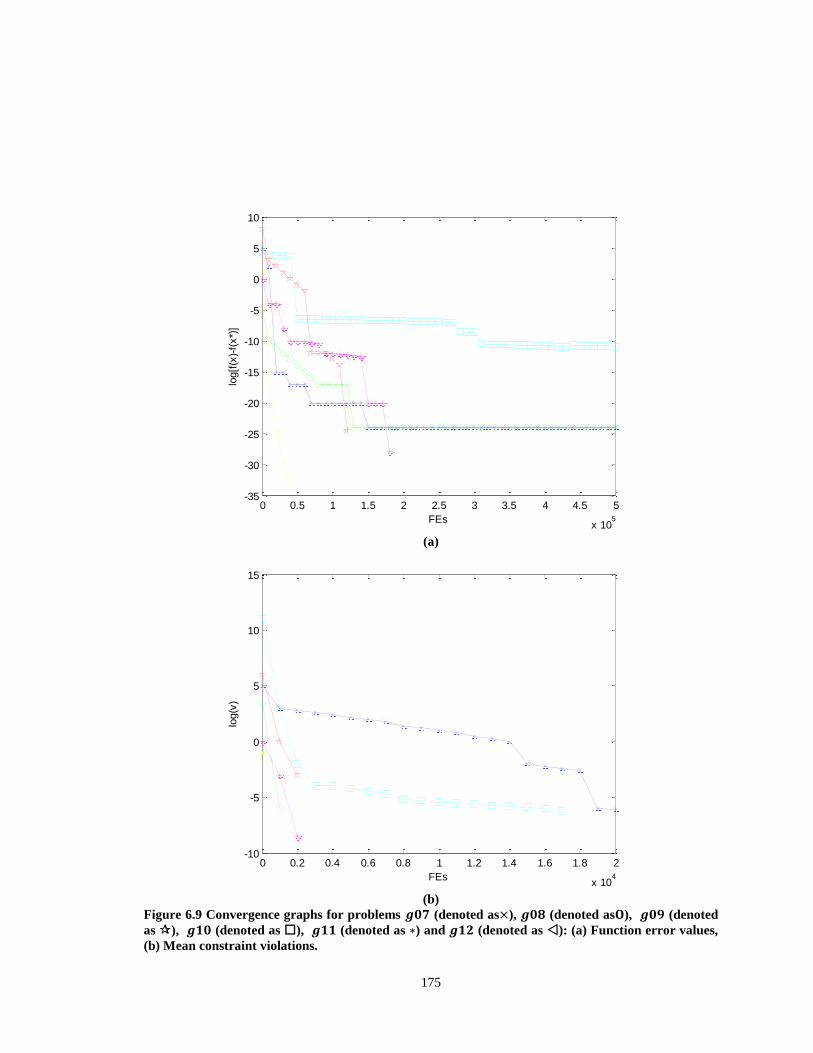
175

(a)

(b)




0 0.5 1 1.5 2 2.5 3 3.5 4 4.5 5

x 105

-35

-30

-25

-20

-15

-10

-5

0

5

10

FEs

log[f

(x)-

f(x*)

]

0 0.2 0.4 0.6 0.8 1 1.2 1.4 1.6 1.8 2

x 104

-10

-5

0

5

10

15

FEs

log(v

)

176

(a)

(b)




0 0.5 1 1.5 2 2.5 3 3.5 4 4.5 5

x 105

-25

-20

-15

-10

-5

0

5

FEs

log[f

(x)-

f(x*)

]

0 0.5 1 1.5 2 2.5 3 3.5 4 4.5

x 104

-6

-4

-2

0

2

4

6

FEs

log(v

)

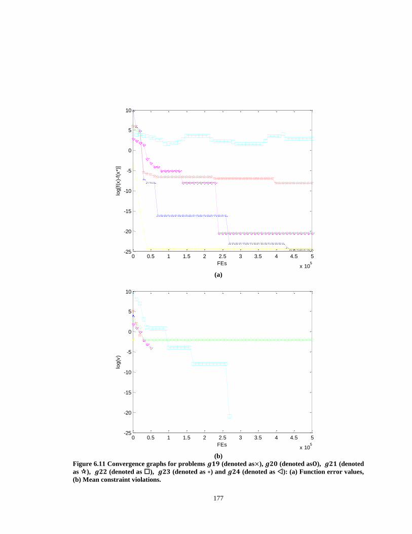
177

(a)

(b)




0 0.5 1 1.5 2 2.5 3 3.5 4 4.5 5

x 105

-25

-20

-15

-10

-5

0

5

10

FEs

log[f

(x)-

f(x*)

]

0 0.5 1 1.5 2 2.5 3 3.5 4 4.5 5

x 105

-25

-20

-15

-10

-5

0

5

10

FEs

log(v

)

178

6.4.5 Algorithm Complexity

In Table 6.9, the algorithm’s complexity corresponding to all 24 benchmark

problems are shown. The computed times in seconds for complexity are , , and

where is defined as:

, (6.24)

where is the computing time of 10,000 evaluations for problem , and is also

defined as:

, (6.25)

where is the complete computing time for the algorithm with 10,000 evaluations for

problem [147]. The running times shown in this table are related to the time spent in

belief space, population space, acceptance function and influence functions.

Table 6.9 Computational complexity

6.2351 11.3280 0.8168

6.4.6 Performance Comparison

Furthermore, the performance of the cultural CPSO has been compared with ten

state-of-the-art constrained optimization heuristics using their best-achieved reported

results in terms of two performance indicators, feasible rate and success rate. The

selected high-performance algorithms are PSO [148], DMS-PSO [149], _DE [150],

GDE [151], jDE-2 [152], MDE [153], MPDE [154], PCX [155], PESO+ [156], SaDE

179

[157]. The comparative results are then demonstrated in Tables 6.10 and 6.11 for feasible

rate and success rate, respectively. The average performance for each algorithm is also

computed. Table 6.10 demonstrate that cultural CPSO has the average feasible rate of

95.83% on 24 benchmark problems that places it at top performing algorithm along with

DMS-PSO [149], _DE [150] and SaDE [157]. Results in Table 6.11 indicate that

proposed cultural CPSO has the average success rate of 90.00% on 24 benchmark

problems placing it at the third best performing algorithm after _DE and PCX [155] with

91.67% and 90.17% of success rate, respectively.

6.4.7 Sensitivity Analysis

In this subsection, the sensitivity of the algorithm performance with respect to

some parameters is briefly assessed. The parameters to be tuned in the proposed

algorithm are the personal acceleration, , swarm acceleration, , global acceleration,

and the rate for information exchange among swarms, . Notice that the allowance

number of particles to migrate, , is a fraction of the population size and does

not need to be tuned. The tolerance for equality constraints is considered a fixed number

of 0.0001 to be able to fairly compare the results of the proposed algorithm with those of

other algorithms. The flight momentum is also randomly selected from a uniform

distribution and does not have tuning issue, and maximum velocity of the particles in

specific dimension depends on the particle’s positional range, consequently will not be

adjusted either.

180

Table 6.10 Comparison of cultural CPSO with the state-of-the-art constrained optimization methods

in terms of feasible rate

Prob. PSO

[148]

DMS-

PSO

[149]

_DE

[150]

GDE

[151]

jDE-2

[152]

MDE

[153]

MPDE

[154]

PCX

[155]

PESO+

[156]

SaDE

[157]

Cultural

CPSO

100% 100% 100% 100% 100% 100% 100% 100% 100% 100% 100%

100% 100% 100% 100% 100% 100% 100% 100% 100% 100% 100%

100% 100% 100% 96% 100% 100% 100% 100% 100% 100% 100%

100% 100% 100% 100% 100% 100% 100% 100% 100% 100% 100%

100% 100% 100% 96% 100% 100% 100% 100% 100% 100% 100%

100% 100% 100% 100% 100% 100% 100% 100% 100% 100% 100%

100% 100% 100% 100% 100% 100% 100% 100% 100% 100% 100%

100% 100% 100% 100% 100% 100% 100% 100% 100% 100% 100%

100% 100% 100% 100% 100% 100% 100% 100% 100% 100% 100%

100% 100% 100% 100% 100% 100% 100% 100% 100% 100% 100%

100% 100% 100% 100% 100% 100% 100% 100% 100% 100% 100%

100% 100% 100% 100% 100% 100% 100% 100% 100% 100% 100%

100% 100% 100% 88% 100% 100% 88% 100% 100% 100% 100%

100% 100% 100% 100% 100% 100% 100% 100% 100% 100% 100%

100% 100% 100% 100% 100% 100% 100% 100% 100% 100% 100%

100% 100% 100% 100% 100% 100% 100% 100% 100% 100% 100%

100% 100% 100% 76% 100% 100% 96% 100% 100% 100% 100%

100% 100% 100% 84% 100% 100% 100% 100% 100% 100% 100%

100% 100% 100% 100% 100% 100% 100% 100% 100% 100% 100%

0% 0% 0% 0% 4% 0% 0% 0% 0% 0% 0%

8% 100% 100% 88% 100% 100% 100% 100% 100% 100% 100%

0% 100% 100% 0% 0% 0% 0% 0% 0% 100% 100%

100% 100% 100% 88% 100% 100% 100% 100% 96% 100% 100%

100% 100% 100% 100% 100% 100% 100% 100% 100% 100% 100%

Average 87.83% 95.83% 95.83% 88.17% 91.83% 91.67% 91.00% 91.67% 91.50% 95.83% 95.83%

A sensitivity analysis has been applied to a selected set of benchmark problems

by varying one parameter at a time while the other parameters are set as values in Table

6.1. Test functions , , , , and have been selected for which the

feasibility and success rate are extremely well or very well, therefore the comparison can

be done by changing tuning parameters. Tables 6.12 to 6.15 show the results of the

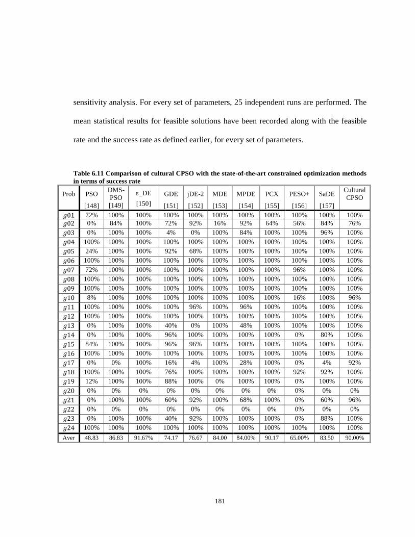
181

sensitivity analysis. For every set of parameters, 25 independent runs are performed. The

mean statistical results for feasible solutions have been recorded along with the feasible

rate and the success rate as defined earlier, for every set of parameters.

Table 6.11 Comparison of cultural CPSO with the state-of-the-art constrained optimization methods

in terms of success rate

Prob PSO

[148]

DMS-

PSO

[149]

_DE

[150]

GDE

[151]

jDE-2

[152]

MDE

[153]

MPDE

[154]

PCX

[155]

PESO+

[156]

SaDE

[157]

Cultural

CPSO

72% 100% 100% 100% 100% 100% 100% 100% 100% 100% 100%

0% 84% 100% 72% 92% 16% 92% 64% 56% 84% 76%

0% 100% 100% 4% 0% 100% 84% 100% 100% 96% 100%

100% 100% 100% 100% 100% 100% 100% 100% 100% 100% 100%

24% 100% 100% 92% 68% 100% 100% 100% 100% 100% 100%

100% 100% 100% 100% 100% 100% 100% 100% 100% 100% 100%

72% 100% 100% 100% 100% 100% 100% 100% 96% 100% 100%

100% 100% 100% 100% 100% 100% 100% 100% 100% 100% 100%

100% 100% 100% 100% 100% 100% 100% 100% 100% 100% 100%

8% 100% 100% 100% 100% 100% 100% 100% 16% 100% 96%

100% 100% 100% 100% 96% 100% 96% 100% 100% 100% 100%

100% 100% 100% 100% 100% 100% 100% 100% 100% 100% 100%

0% 100% 100% 40% 0% 100% 48% 100% 100% 100% 100%

0% 100% 100% 96% 100% 100% 100% 100% 0% 80% 100%

84% 100% 100% 96% 96% 100% 100% 100% 100% 100% 100%

100% 100% 100% 100% 100% 100% 100% 100% 100% 100% 100%

0% 0% 100% 16% 4% 100% 28% 100% 0% 4% 92%

100% 100% 100% 76% 100% 100% 100% 100% 92% 92% 100%

12% 100% 100% 88% 100% 0% 100% 100% 0% 100% 100%

0% 0% 0% 0% 0% 0% 0% 0% 0% 0% 0%

0% 100% 100% 60% 92% 100% 68% 100% 0% 60% 96%

0% 0% 0% 0% 0% 0% 0% 0% 0% 0% 0%

0% 100% 100% 40% 92% 100% 100% 100% 0% 88% 100%

100% 100% 100% 100% 100% 100% 100% 100% 100% 100% 100%

Aver

age

48.83

%

86.83

%

91.67% 74.17

%

76.67

%

84.00

%

84.00% 90.17

%

65.00% 83.50

%

90.00%

182

The results in Tables 6.12 to 6.14 show the effect of varying the personal, swarm

and global acceleration on the algorithm’s performance. It seems that the effect of

varying the acceleration on algorithm’s performance is by some extent, problem-

dependent. This makes it difficult to identify the optimum parameters in order to achieve

the best performance.

Table 6.12 Sensitivity analysis with respect to personal acceleration, : Mean results of feasible

solutions, Feasible Rate and Success Rate are computed over 25 independent runs.

Prob.

Mean results of feasible solutions, Feasible Rate, Success Rate

1.0 1.5 2.0 2.5

-1.0005001000,

100%,100%

-1.0005001000,

100%,100%

-1.0005001000,

100%,100%

-1.0005001000,

100%,100%

7049.248020570674,

100%,96%

7049.248020573664,

100%,96%

7049.248020573941,

100%,100%

7049.248020570062,

100%,96%

-47.7648884595,

100%,100%

-47.7648884595,

100%,100%

-47.7648884595,

100%,100%

-47.7648884595,

100%,92%

-0.8660254038,

100%,100%

-0.8660254038,

100%,100%

-0.8660254038,

100%,96%

-0.8660254038,

100%,100%

193.7245128803,

100%,96%

193.7245126309,

100%,96%

193.7245121603,

100%,100%

193.7245139367,

100%,92%

We suggest further analyzing this issue and implementing an adaptive dynamic

law based upon the need for exploration or exploitation in the f-v space discussed in

spatial knowledge of the belief space. This approach is similar to the one introduced in

[140-141]. The results in Table 6.16 show that by increasing the rate for information

exchange, the success rate will be greatly improved for all selected benchmark problems.

On the other hand by decreasing this rate, the success rate gets deteriorate.

183

Table 6.13 Sensitivity analysis with respect to swarm acceleration, : Mean results of feasible


Prob.


1.0 1.5 2.0 2.5

-1.0005001000,

100%,100%

-1.0005001000,

100%,100%

-1.0005001000,

100%,100%

-1.0005001000,

100%,100%

7049.248020574453,

100%,100%

7049.248020573664,

100%,96%

7049.248020579940,

100%,96%

7049.248020573296,

100%,96%

-47.7648884595,

100%,100%

-47.7648884595,

100%,100%

-47.7648884595,

100%,100%

-47.7648884595,

100%,100%

-0.8660254038,

100%,96%

-0.8660254038,

100%,100%

-0.8660254038,

100%,100%

-0.8660254038,

100%,96%

193.7245126006,

100%,100%

193.7245126309,

100%,96%

193.7245124569,

100%,100%

193.7245124389,

100%,96%

6.5 Discussions

In this chapter, the cultural CPSO, a novel heuristic to solve constrained

optimization problems has been proposed which incorporates information of objective

function and constraints violation, to construct a cultural framework consisting two

sections: a multiple swarm PSO with the ability of inter-swarm communication as

population space and a belief space including four sections, normative knowledge, spatial

knowledge, situational knowledge, and temporal knowledge. Each swarm assembles two

lists of particles to share with other swarms based upon cultural information retrieved

from different sections of the belief space. This cultural-based communication facilitates

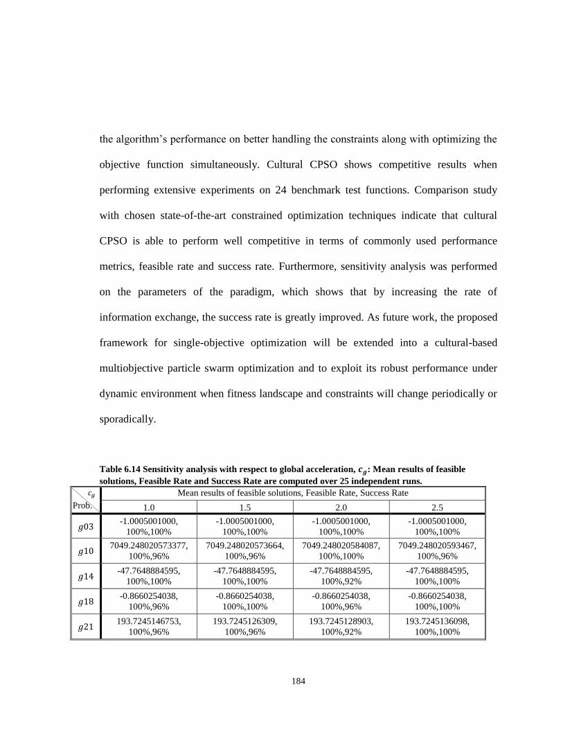
184

the algorithm’s performance on better handling the constraints along with optimizing the

objective function simultaneously. Cultural CPSO shows competitive results when

performing extensive experiments on 24 benchmark test functions. Comparison study

with chosen state-of-the-art constrained optimization techniques indicate that cultural

CPSO is able to perform well competitive in terms of commonly used performance

metrics, feasible rate and success rate. Furthermore, sensitivity analysis was performed

on the parameters of the paradigm, which shows that by increasing the rate of

information exchange, the success rate is greatly improved. As future work, the proposed

framework for single-objective optimization will be extended into a cultural-based

multiobjective particle swarm optimization and to exploit its robust performance under

dynamic environment when fitness landscape and constraints will change periodically or

sporadically.

Table 6.14 Sensitivity analysis with respect to global acceleration, : Mean results of feasible


Prob.


1.0 1.5 2.0 2.5

-1.0005001000,

100%,100%

-1.0005001000,

100%,100%

-1.0005001000,

100%,100%

-1.0005001000,

100%,100%

7049.248020573377,

100%,96%

7049.248020573664,

100%,96%

7049.248020584087,

100%,100%

7049.248020593467,

100%,96%

-47.7648884595,

100%,100%

-47.7648884595,

100%,100%

-47.7648884595,

100%,92%

-47.7648884595,

100%,100%

-0.8660254038,

100%,96%

-0.8660254038,

100%,100%

-0.8660254038,

100%,96%

-0.8660254038,

100%,100%

193.7245146753,

100%,96%

193.7245126309,

100%,96%

193.7245128903,

100%,92%

193.7245136098,

100%,100%

185

Table 6.15 Sensitivity analysis with respect to rate of information exchange, : Mean results of

feasible solutions, Feasible Rate and Success Rate are computed over 25 independent runs.

Prob.


10% 20% 30% 40%

-1.0005001000,

100%,92%

-1.0005001000,

100%,100%

-1.0005001000,

100%,100%

-1.0005001000,

100%,100%

7049.248020692614,

100%,92%

7049.248020579157,

100%,96%

7049.248020573664,

100%,96%

7049.248020550004,

100%,100%

-47.7648884586,

100%,96%

-47.7648884595,

100%,100%

-47.7648884595,

100%,100%

-47.7648884595,

100%,100%

-0.8660254017,

100%,96%

-0.8660254038,

100%,100%

-0.8660254038,

100%,100%

-0.8660254038,

100%,100%

193.7245268306,

100%,92%

193.7245138506,

100%,96%

193.7245126309,

100%,96%

193.7245110215,

100%,100%

186

CHAPTER VII

DYNAMIC OPTIMIZATION USING CULTURAL-BASED PARTICLE SWARM

OPTIMIZATION

7.1 Introduction

Many real-world optimization problems are dynamic thus the optimum solution

changes in time. In such cases, the optimization algorithm should detect the change and

respond to the change promptly. Examples of dynamic optimization problems include

jobs scheduling, changing profits in portfolio optimization, and fluctuating demand.

There are four major categories of uncertainties that have been dealt with using

population based evolutionary approaches: noise in the fitness function, perturbations in

the design variables, approximation in the fitness function, and dynamism in optimal

solutions [12]. While noise and approximation bring uncertainty in the objective function,

perturbation introduces uncertainty in the decision space. This study is focused on

dynamic optimization problems (DOPs), formulated as:

Optimize ),,( ef x (7.1)

187

where ),...,,( 21 Mxxxx is the M-dimensional decision variable limited in each dimension

as max,min, jjj xxx (for Mj ,...,2,1 ), f is the objective function, e represents the

possible change in the objective function, constraints, environmental parameters, or

problem representations during optimization process. As a result these changes

represented by parameter e may affect the height, width, or location of optimum solution

or a combination of these three parts [13]. For the simplicity purposes, this study is

performed on the minimization problems. Note that a maximization problem can be

converted to a minimization problem simply using multiplication by –1.

One common example of DOPs is job shop scheduling problems in which new

jobs arrive or machines may break down during operations resulting a need for dynamic

job schedules to accommodate the changes over time [10]. Another example of DOPs is

dynamic portfolio problem in which the goal is to obtain an optimal allocation of assets

to maximize profit and minimize investment risk [11]. Dynamic portfolio management

can also be observed in coordinating different power stations in order to maximize profit

and minimize risk. Some of the uncertainties here include spot market prices, load

obligations, and strip/option prices. Practically speaking, optimization can be needed for

the market price as often as every hour [11].

Population based heuristic had been adopted to solve optimization problems with

dynamic landscape in the last few years. Particle swarm optimization (PSO) [1] is a

popular population based paradigms introduced within the last decade. PSO mimics

188

behavior of the flocking birds by introducing a simple particle flight mechanism as:

)),()(())()(()()1( 21 txtgbestrctxtpbestrctwvtv d

i

d

g

d

i

d

ip

d

i

d

i (7.2)

),1()()1( tvtxtx d

i

d

i

d

i (7.3)

where )(txd

iis the d-th dimension of the position of the i-th particle at time t

( Ni ,...,2,1 and Md ,...,2,1 , where N is number of particles and M is the decision

space dimension). )(tvd

i is the d-th dimension of the velocity of the i-th particle at time t .

)(tpbestd

iis the d-th dimension of the personal best position of the i-th particle at time t ,

and )(tgbestd is the d-th dimension of the global best position at time t . pc and gc are

the constant personal and global acceleration which give different importance weight to

personal or global term of (7.2). 1r and 2r are uniform random numbers from (0,1) to give

stochastic characteristics to the flight of particles. w is the velocity inertia weight of the

particles. The application of PSO to dynamic optimization problems has been studied by

various researchers [10, 44, 84-98, 158-163]. There are some issues with the PSO

mechanism that needs to be addressed. One of them is the outdated memory in a sense

that if the problem changes, a previously good solution stored as neighborhood or

personal best may no longer be good, and will mislead the swarm towards false optima if

the memory is not updated. The other issue is diversity loss. The population should

189

normally collapse around the best solution found during the optimization. In dynamic

optimization, the partially converged population after a change is detected should quickly

re-diversify, find the new optimum and re-converge quickly [10]. A number of

adaptations have been applied to PSO in order to solve these deficiencies; memories can

be refreshed or forgotten and swarms may be re-diversified through randomization, or

exchange of information using multi-swarms.

In general, a good evolutionary heuristic to solve DOPs should be able to track

the changing optimal solution even under high severity and frequency of change. It must

reuse as much information as possible from previous generations to enhance the

optimization search. Among the researches performed in dynamic PSO none of these

studies use information from all particles to perform re-diversification through migration

and repulsion. When particles share their information through migration process, they

will be able to quickly re-diversify and move efficiently towards new optimum by re-

converging around it. In order to construct the environment required for this re-

divergence and re-convergence, we need to build groundwork to assist us to utilize this

information. The major groundwork is the belief space of cultural algorithm assisting the

particles in an organized informational manner to locate the necessary information.

Through psychosocial literature, studies show that attitudinal similarity leads to

attraction while dissimilarity leads to repulsion in interpersonal relationship [14],

consequently people often diverge from members of other social groups by selecting

cultural tastes (e.g., possessions, attitudes, or behaviors) that distinguish them from

190

others. For example, a field study has found that students stopped wearing a particular

wristband when members of a geeky dormitory next door started wearing them [15].

Indeed different cultural beliefs lead to repulsion and increase the possibilities of

divergence in ideas and in turn open up the doors to new opportunities.

Computationally speaking, one difficulty is to find the proper information to adopt in

order to rely on a quick re-diversification when a change happens in the environment.

Using many concepts from the cultural algorithm, such as spatial knowledge, temporal

knowledge, domain knowledge, normative knowledge and situational knowledge, we will

be able to efficiently and effectively organize the available knowledge to adopt in several

steps of the PSO’s updating mechanism as well as re-diversification and repulsion among

swarms. The special re-diversification problem to deal with the change in dynamic is an

important task that cannot be solved unless we have access to the knowledge throughout

the search process that is performed by the cultural algorithm as the computational

framework.

In this study, a novel computational framework based on cultural algorithm has

been proposed using knowledge stored in the belief space to re-diversify the population

right after a change takes place in the dynamic of the problem. Thus the algorithm can

comfortably compute the repulsion factor for each particle and locate the leading particles

in the personal level, swarm level and global level. Each particle in the proposed cultural-

based dynamic PSO will fly through a mechanism of three level flight incorporated with

a repulsion factor. After a change takes place, particles regroup into several swarms and a

191

diversity-based migration among swarms along with repulsive mechanism implemented

in repulsion factor will take place to increase the diversity as quickly as possible. The

remaining sections of this chapter to complete the presentation are as following. In

Section 7.2, related works in dynamic PSO and related research in cultural algorithm

have been reviewed. Section 7.3 includes a detailed description of the proposed cultural-

based dynamic PSO. In Section 7.4, simulation results are evaluated on the benchmark

test problems in comparison with the state-of-the-art paradigms. Lastly, Section 7.5

summarizes the concluding remarks and future work of this study.


7.2.1 Related Work in Dynamic PSO

Relevant works of particle swarm optimization that had been adopted to solve

DOPs are briefly discussed in this subsection in order to motivate the proposed ideas.

Particle swarm optimization has demonstrated its ability to solve the dynamic

optimization problems. Carlisle and Dozier [84] adjusted PSO mechanism so it avoids

making position/velocity decision based on the outdated memory. They introduced

periodic resetting by having the particles periodically replace their pbest vector with their

current position, forgetting their past experiences. They also introduced triggered

resetting in which particles reset when the goal moves some specific distance from its

original position. Eberhart and Shi [44] proposed that when perturbation is small, the

192

initialization of the swarm can start from old population, while with large perturbation, it

would be better to re-initialize and then compare the results with the old swarm and select

the best one. Hu and Eberhart [85] introduced a detection and response paradigm for PSO

to solve dynamic problems in which gbest and the second global best are evaluated to

monitor the changes. As to respond, the whole particles’ positions are re-randomized.

Blackwell and colleages proposed charged swarm to avoid collision among particles

based upon the force between electric charges which is inversely proportional to distance

squared [86]. In a later work, the atomic model of PSO [87] and quantum PSO [88] are

introduced in which the particles follow the structure of the chemical atom including a

cloud of electrons randomly orbiting with a specific radius around the nucleolus. They

have applied their models into multiple swarm PSO to solve multiple peak dynamic

function problem [88], outperforming other evolutionary algorithm based heuristics. An

anti-convergence operator is introduced [89] for swarms to interact with each other. Also

an excluding operation is performed on swarms with their best solutions within a

predefined radius. The nearby swarms compete with each other in order to promote

diversity. The winner, the swarm with the best function value at its swarm attractor, will

remain, while the loser will be re-initialized in the search space [89]. Blackwell [90]

proposed swarms birth and death by allowing multiple swarms to regulate their size by

bringing new swarms to existence, or diminishing redundant swarms. This dynamic

swarm size removes the need for anti-convergence and exclusion operators in the PSO

mechanism.

193

Brabazon and colleagues [158] adapted particle swarm metaphor in the domain of

organizational adaptation in the presence of uncertainty. Strategic adaptation is

considered as an attempt to uncover peaks on a high-dimensional strategic landscape.

Some strategic configurations produce high profits, others produce poor results. A model

is also adopted to estimate the noise incorporated in the strategy fitness. Janson and

Middendorf [91] proposed partitioned hierarchical PSO for dynamic optimization

problems. In their model, the population is partitioned into some tree-form sub-

hierarchies for a limited number of iterations after a change is detected. These sub-

hierarchies continue to independently search for the optimum, resulting a wider spread-

out of the search process after the change has occurred. The topmost level of tree-form

hierarchies which contain the current best particle does not change, but all lower sub-

hierarchies (sub-swarms) by re-initializing the position and velocity and resetting their

personal best positions. These sub-hierarchies are rejoined again after a predefined

number of iterations. In a later work [159] a function re-evaluation paradigm is added to

handle the noise. In this work, change detection mechanism for noisy environment is also

proposed based upon observing the changes occurring within the hierarchy.

Venayagamoorthy [160] adopted adaptive critic design (ACD) to handle DOP

problems using particle swarm. The dynamic change in this study is caused in the inertia

weight with the goal to optimize the objective function. Two neural networks of the

ACD, namely Critic network and Action network, will receive the inputs as the inertia

weight and the fitness value for gbest of the current iteration respectively. The objective

194

of the Action network is to minimize the output of the Critic network by varying the

inertia weight to improve the gbest fitness. Esquivel and Coello Coello [92] proposed a

dynamic macro-mutation operator along with PSO to maintain the diversity throughout

the search process in order to solve DOPs. Every coordinate of each particle will undergo

an independent mutation with a dynamic probability which possess its highest value

when the change occurs in the dynamic landscape and gradually decreases till the next

change takes place.

Parsopoulos and Vrahatis [93] adopted their proposed unified PSO in dynamic

environments. The unified PSO combines the exploration and exploitation term of the

PSO mechanism into a unification factor to balance the influence of the global and local

search directions. Zhang et al. [94] proposed a direct relation between the inertia weight

of the particle and the change. In their model, the new gbest and pbest for each particle

affect the inertia weight of the particle whenever a change in gbest or pbest occurs. Pan et

al. [95] modified the PSO paradigm using a probability based movement of particles

based upon the concept of energy change probability in Simulated Annealing (SA). The

particle will move to the next position computed through traditional PSO heuristics only

with a specific probability that exponentially depends on the difference between the

objective values of the current and next iterations.

Trojanowski proposed quantum particles in multi-swarm to solve dynamic

optimization tasks. His two-phase paradigm includes computing an angle and a distance

for the new location of the particles. The proposed method allows the locations to be

195

distributed over the entire search space. The angle is obtained from an angularly uniform

distribution on the surface of a hyper-sphere while the distance is an α-stable random

variate [161]. Parrott and Li [96] proposed species based PSO for solving dynamic

optimization problems. The population is divided into some swarms, each surrounding a

dominating particle called species seeds which are identified from the entire population

based upon their objective function values. The new seed should not fall within the

predefined radius of all previously found seeds in order to promote diversity. The seeds

are then selected as the neighborhood best for different swarms. In a later work, Li and

colleagues [10, 162-163] included quantum particles into species based PSO to promote

more diversity along with the re-randomization of the worst species.

Du and Li [97] introduced multi-strategy ensemble PSO in which particles are

divided into two sections, part I uses a Gaussian local search to quickly seek global

optimum in the current environment, while part II uses differential mutation to explore

the search space. The position of particles in part II do not follow the traditional PSO

mechanism, instead each particle in part II is determined by the particle in part I through

a mutation strategy. There is 50% chance of getting closer to a randomly chosen pbest

particles or going farther away from that pbest. Liu et al. [98] introduced a modified PSO

to solve DOPs. In the proposed model, PSO consists of many compound particles. Each

compound particle includes three single particles equilaterally distanced from each other

in a triangular shape. A special reflection scheme is proposed to explore the search space

more comprehensively in which the position of the worst particle among three in the

196

compound will be replaced with the reflected one. In each compound particle, after

reflection is performed, a representative among these three particles is probabilistically

chosen based upon the objective function values and distance from other two member

particles. The representative member particles will then participate in PSO update

mechanism. The two non-representative particles will also move the same

distance/direction as representative particle has been moved in order to preserve the

valuable information.

7.2.2 Related Works in Cultural Algorithm for Dynamic Optimization

Reynolds [3] proposed cultural algorithm (CA) as a double interconnecting

heritage system in which information passed along to the next iteration through two

interconnecting spaces, population and belief space. Defining culture as information

storage in a broader than individual level which is accessible by all society members, CA

tries to mimic it through its belief space scheme [99]. CA has shown its ability to solve

different types of problems including dynamic optimization problems [106, 164].

Cultural framework had also been successfully adopted to assist particle swarm

optimization to solve multiobjective optimization problems [140-141], and constrained

optimization problems [165].

7.3 Cultural Particle Swarm for Dynamic Optimization

197

A summary of the pseudocode of the proposed paradigm is depicted in Figure 7.1

and a block diagram representation of the proposed algorithm is demonstrated in Figure

7.2. The population space (PSO) will be initialized and then divided into several swarms

according to the closeness of the particles. The belief space (BLF) is then initialized. We

evaluate population space using the objective function values. Next we apply acceptance

function to select some particles which will be later adopted for the belief space. Belief

space consists of five sections, situational, temporal (or history), domain, normative and

spatial (topographical) knowledge. This cultural framework plays a key role in the

heuristics. Next we apply influence functions to the belief space in order to select the key

parameters of PSO for next iteration, including the repulsion factor for each particle,

personal best, swarm best and global best. Through a scheme using information from a

belief space, the change in dynamic will be detected. As soon as the change is detected,

influence function applies to the belief space to perform the repulsive diversity-promoted

migration among swarms. This migration will take place using the information extracted

from the belief space. Then particles in the population space fly using newly computed

repulsion factor, personal, swarm, and global best. This process continues until the

stopping criteria are met.

In the remainder of this section, thorough explanation of the multi-swarm

divergence-promoted population space, acceptance function, different parts of belief

space including situational, temporal, domain, normative and spatial knowledge,

influence functions including change-driving diversity-based migration are presented.

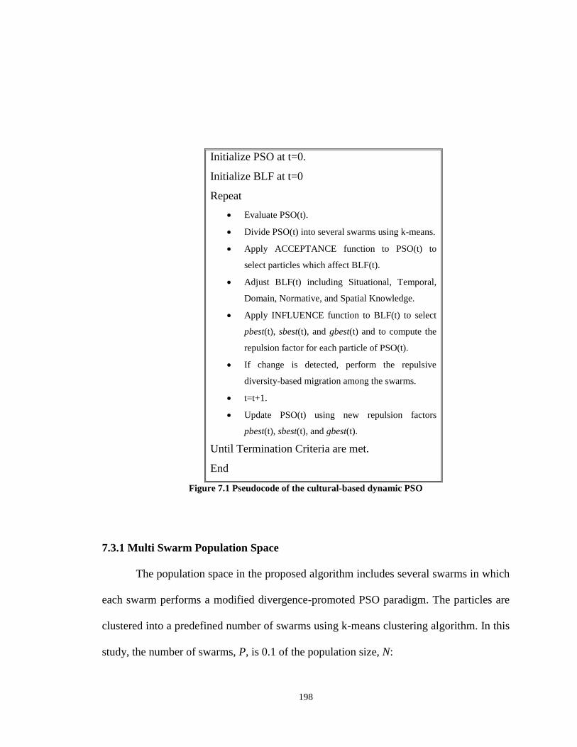
198

Initialize PSO at t=0.

Initialize BLF at t=0

Repeat

Evaluate PSO(t).

Divide PSO(t) into several swarms using k-means.

Apply ACCEPTANCE function to PSO(t) to

select particles which affect BLF(t).

Adjust BLF(t) including Situational, Temporal,

Domain, Normative, and Spatial Knowledge.

Apply INFLUENCE function to BLF(t) to select

pbest(t), sbest(t), and gbest(t) and to compute the

repulsion factor for each particle of PSO(t).

If change is detected, perform the repulsive

diversity-based migration among the swarms.

t=t+1.

Update PSO(t) using new repulsion factors

pbest(t), sbest(t), and gbest(t).

Until Termination Criteria are met.

End

Figure 7.1 Pseudocode of the cultural-based dynamic PSO

7.3.1 Multi Swarm Population Space

The population space in the proposed algorithm includes several swarms in which

each swarm performs a modified divergence-promoted PSO paradigm. The particles are

clustered into a predefined number of swarms using k-means clustering algorithm. In this

study, the number of swarms, P, is 0.1 of the population size, N:

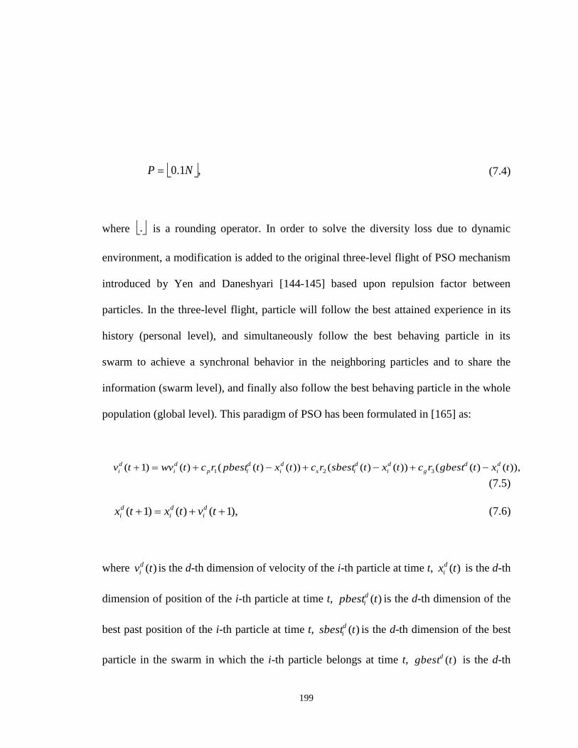
199

,1.0 NP (7.4)

where . is a rounding operator. In order to solve the diversity loss due to dynamic

environment, a modification is added to the original three-level flight of PSO mechanism

introduced by Yen and Daneshyari [144-145] based upon repulsion factor between

particles. In the three-level flight, particle will follow the best attained experience in its

history (personal level), and simultaneously follow the best behaving particle in its

swarm to achieve a synchronal behavior in the neighboring particles and to share the

information (swarm level), and finally also follow the best behaving particle in the whole

population (global level). This paradigm of PSO has been formulated in [165] as:

)),()(())()(())()(()()1( 321 txtgbestrctxtsbestrctxtpbestrctwvtv d

i

d

g

d

i

d

is

d

i

d

ip

d

i

d

i

(7.5)

),1()()1( tvtxtx d

i

d

i

d

i (7.6)

where )(tvd

i is the d-th dimension of velocity of the i-th particle at time t, )(txd

i is the d-th

dimension of position of the i-th particle at time t, )(tpbestd

i is the d-th dimension of the

best past position of the i-th particle at time t, )(tsbestd

i is the d-th dimension of the best

particle in the swarm in which the i-th particle belongs at time t, )(tgbestd is the d-th

200

dimension of the best particle of population at time t. 1r , 2r , and 3r are uniformly

generated random numbers in the range of (0,1), pc , sc , and

gc are constant values

representing the weight for personal, swarm, and global behavior and w is the

momentum for previous velocity. The swarm flight, Equations (7.5) and (7.6), has been

modified to promote diversity after a change is detected as following:

,)()(

)()(

)()())()((

))()(())()(()()1(

133

21

N

ijj

jidj

di

dj

did

id

g

di

dis

di

dip

di

di

tQtQ

txtx

txtxtxtgbestrc

txtsbestrctxtpbestrctwvtv

(7.7)

).1()()1( tvtxtx d

i

d

i

d

i (7.8)

The forth term in the above equation is called the repulsive term and is

incorporated into the dynamic of the particles in the swarm based upon the psychosocial

studies. The psychological research shows that dissimilarity leads to repulsion in

interpersonal relationship [14]. As a result people often diverge from members of other

social groups by selecting cultural tastes (e.g., possessions, attitudes, or behaviors) that

distinguish them from others [15]. A repulsion factor is added to all particles in the

population space as a modified version of charged PSO. In charged PSO, some particles

are considered as charged with fixed charges that repel from other charged particles

according to the coulomb law [86]. In the modified version proposed here, )(tQi and

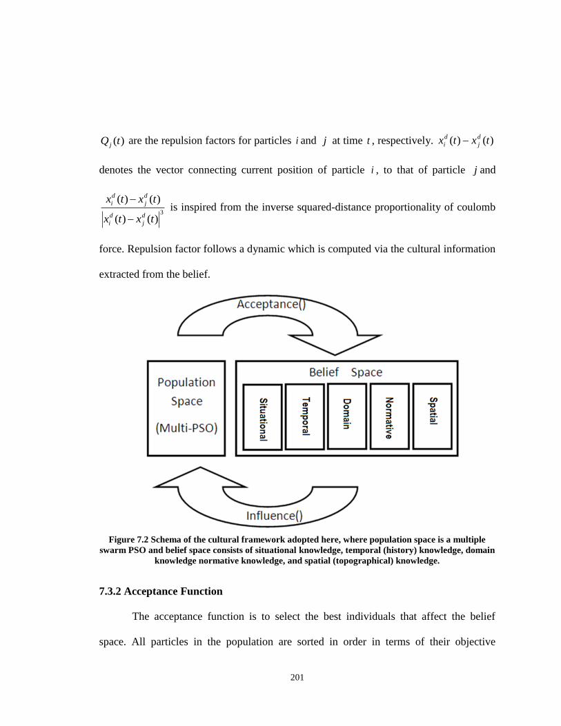
201

)(tQ j are the repulsion factors for particles i and j at time t , respectively. )()( txtx d

j

d

i

denotes the vector connecting current position of particle i , to that of particle j and

3

)()(

)()(

txtx

txtx

d

j

d

i

d

j

d

i

is inspired from the inverse squared-distance proportionality of coulomb

force. Repulsion factor follows a dynamic which is computed via the cultural information

extracted from the belief.

Figure 7.2 Schema of the cultural framework adopted here, where population space is a multiple

swarm PSO and belief space consists of situational knowledge, temporal (history) knowledge, domain

knowledge normative knowledge, and spatial (topographical) knowledge.


The acceptance function is to select the best individuals that affect the belief

space. All particles in the population are sorted in order in terms of their objective

202

function values at the current iteration and % of the particles starting from best to worst

are selected, where is a predefined constant value.

7.3.3 Belief Space

The belief space in this paradigm consists of five sections, situational, temporal,

domain, normative and spatial knowledge. In the remainder of this section, the type of

information, represent method of the knowledge and updating methodology of the

knowledge in each section of the belief space are elaborated.


This part of belief space is used to keep the good exemplar particles for each

swarm. Its representation is shown in Figure 7.3. )(ˆ tix ( Pi ,...,2,1 ) where P is the

number of swarms defined in Equation (7.4), is the best particle in the i-th swarm based

upon objective function evaluation. Assume that at an arbitrary iteration the i-th swarm

consists iN particles as

iNzzz ,...,, 21 with correspondent objective functions values as

iNfff ,...,, 21 respectively. Then },...,,{)(ˆ

21 iNi zzzt x is defined such that:

,min)),(ˆ( 1 lNli fetfix ,,...,2,1 Pi (7.9)

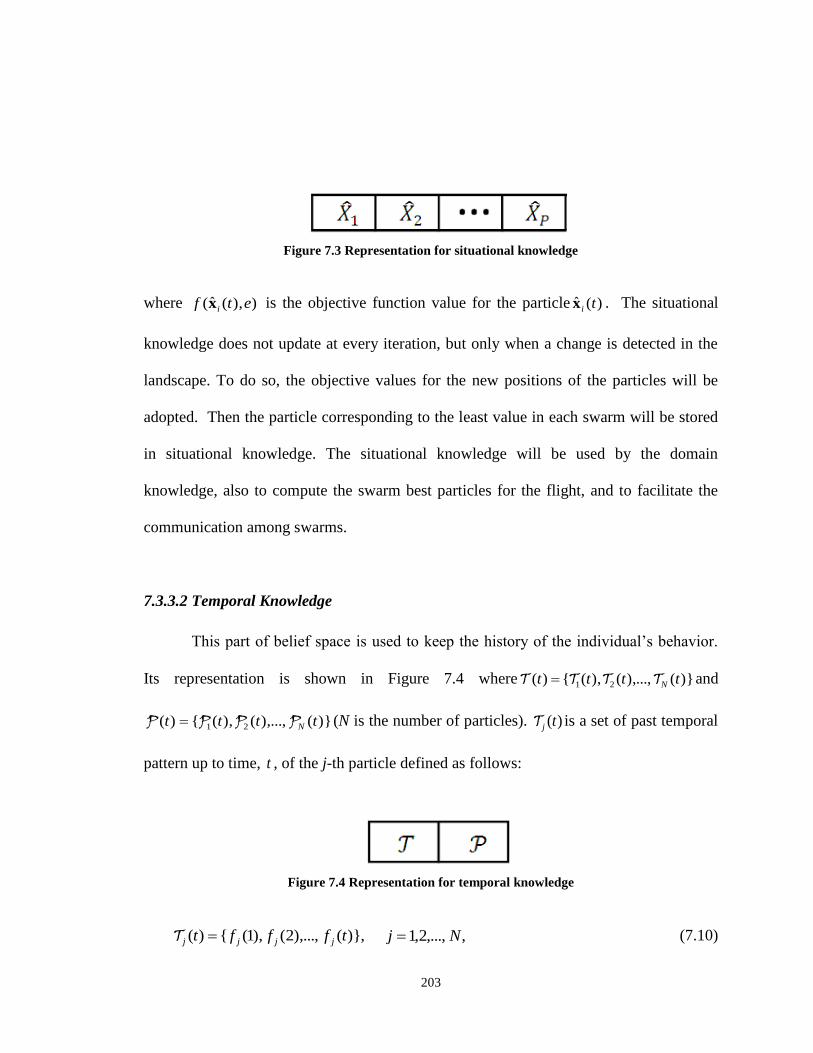
203

Figure 7.3 Representation for situational knowledge

where )),(ˆ( etf ix is the objective function value for the particle )(ˆ tix . The situational

knowledge does not update at every iteration, but only when a change is detected in the

landscape. To do so, the objective values for the new positions of the particles will be

adopted. Then the particle corresponding to the least value in each swarm will be stored

in situational knowledge. The situational knowledge will be used by the domain

knowledge, also to compute the swarm best particles for the flight, and to facilitate the

communication among swarms.

7.3.3.2 Temporal Knowledge

This part of belief space is used to keep the history of the individual’s behavior.

Its representation is shown in Figure 7.4 where )}(),...,(),({)( 21 tttt NTTTT and

)}(),...,(),({)( 21 tttt NPPPP (N is the number of particles). )(tjT is a set of past temporal

pattern up to time, t , of the j-th particle defined as follows:

Figure 7.4 Representation for temporal knowledge

)},(),...,2(),1({)( tffft jjjj T ,,...,2,1 Nj (7.10)

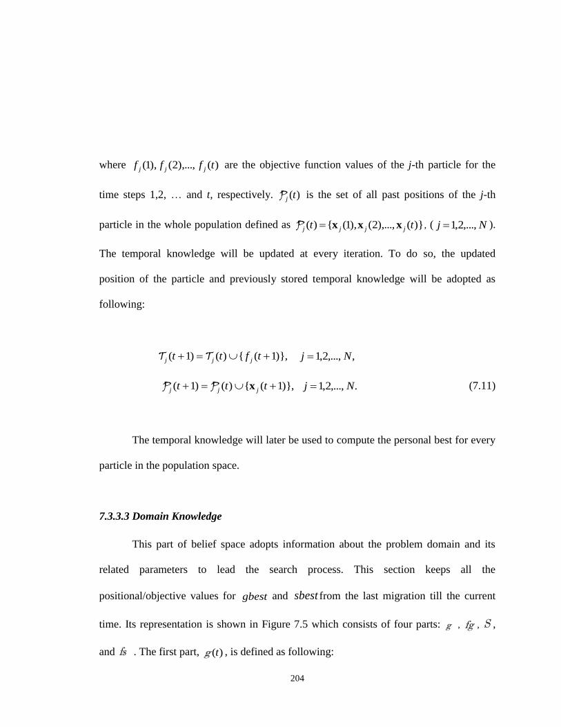
204

where )(),...,2(),1( tfff jjj are the objective function values of the j-th particle for the

time steps 1,2, … and t, respectively. )(tjP is the set of all past positions of the j-th

particle in the whole population defined as )}(),...,2(),1({)( tt jjjj xxxP , ( Nj ,...,2,1 ).

The temporal knowledge will be updated at every iteration. To do so, the updated

position of the particle and previously stored temporal knowledge will be adopted as

following:

)},1({)()1( tftt jjj TT ,,...,2,1 Nj

)},1({)()1( ttt jjj xPP .,...,2,1 Nj (7.11)

The temporal knowledge will later be used to compute the personal best for every

particle in the population space.

7.3.3.3 Domain Knowledge

This part of belief space adopts information about the problem domain and its

related parameters to lead the search process. This section keeps all the

positional/objective values for gbest and sbest from the last migration till the current

time. Its representation is shown in Figure 7.5 which consists of four parts: g , fg , S ,

and fs . The first part, )(tg , is defined as following:

205

},)({)( ttTtgbestt Migration

k g

(7.12)

where Migration

kT denotes the time for the k-th migration (and the last migration before the

current iteration) among swarms ( ,...2,1,0k ), and t is the current iteration, and P is the

number of swarms given by Equation (7.4). ttT Migration

k denotes all the iterations,

t , among the last migration , Migration

kT , and the current time, t . By default it is assumed

that 10 MigrationT . )( tgbest is computed as following:

))},(min()(1),()({)( ttfNjtttgbest jj FPx (7.13)

where )}(),...,(),({)( 21

tttt NxxxP is the whole population of particles at time t , and

)}(),...,(),({)( 21

tftftft NF is a set consisting of the modified objective function

values for all particles at time t . The second part of domain knowledge is )(tfg which is

defined as objective values for each values of the )(tg . Notice that since the objective

function in Equation (7.1) is dynamic, therefore the objective function value for the same

position may not necessarily be identical for two different iterations due to the possible

change of environment. In the domain knowledge we preserve the objective value as:

206

},))(({)( ttTtgbestft Migration

k fg (7.14)

where (.)f is the objective function adopted for the time t , which may not be the same

as (.)f for the current time due to environmental change, e (see Equation (7.1)). The

third section of the domain knowledge is )(tS computed as:

},,...,2,1,)(ˆ{)( PittTtt Migration

ki xS

(7.15)

Figure 7.5 Representation for the domain knowledge

where )(ˆ tix is extracted from the situational knowledge for all such time t between the

last migration, Migration

kT and the current time, t . Finally, the fourth section of the domain

knowledge is )(tfs objective values for each values of the )(tS as following:

},,...,2,1,))(ˆ({)( PittTtft Migration

ki xfs (7.16)

where (.)f is again the objective function used for the time t , not the current time, since

due to dynamic nature of the problem (.)f for the current time might have been different

207

from (.)f for the time t .

The domain knowledge is then updated at every iteration and reset when a

migration among swarms takes place as following:

,1 if ),1(

1 if )},1({)()1(

1

1

Migration

k

Migration

k

Tttgbest

Tttgbesttt

gg

(7.17)

,1 if )),1((

1 if ))},1(({)()1(

1

1

Migration

k

Migration

k

Tttgbestf

Tttgbestftt

fgfg

(7.18)

,1 if },,...,2,1)1(ˆ{

1 if },,...,2,1)1(ˆ{)()1(

1

1

Migration

ki

Migration

ki

TtPit

TtPittt

x

xSS

(7.19)

.1 if },,...,2,1))1(ˆ({

1 if },,...,2,1))1(ˆ({)()1(

1

1

Migration

ki

Migration

ki

TtPitf

TtPitftt

x

xfsfs

(7.20)

This means that if migration does not happen, the new gbest is computed using

Equation (7.13) and will be added to the domain knowledge along with its correspondent

objective values. Also the new information from situational knowledge for the current

iteration, along with their correspondent objective values will be added to update the

domain knowledge. On the other hand if migration takes place then the new gbest is

computed using Equation (7.13) and will be placed as the first part of domain knowledge.

The second part is the objective value this new gbest. The third part of the domain

knowledge is extracted from the current situational knowledge, and finally the fourth part

208

is placed via the objective value for the third part. In this way, the domain knowledge will

be constructed if migration has taken place. The domain knowledge will later be used to

detect the changes of the dynamic landscape of the problem, and also to produce the

required particles for particles’ flights such as global best and swarm best.


In this section of the belief space best areas are adopted to nominate and exchange

among swarms. Its representation is demonstrated in Figure 7.6 which consists two parts

},...,,{ 21 PSSSS and },...,,{ 21 PRRRR where iS ( Pi ,...,2,1 ) denotes a send list

of particles in the i-th swarm which will be selected to be sent to the next swarm, while

iR ( Pi ,...,2,1 ) is a replace list of particles in the i-th swarm to be replaced by particles

coming from another swarm.

Figure 7.6 Representation of normative knowledge

This mechanism to increase diversity has been introduced and adopted by Yen

and Daneshyari [144-145]. This mechanism is used to quickly regain the divergence after

a change is detected in the landscape of the problem. To regain the divergence, each

swarm prepares two lists of particles, a list to be sent to the next swarm and another to be

replaced by particles coming from another swarm. These two sections of normative

209

knowledge is prepared according to the particles’ locations in the swarm and the

objective function values. Assume that at an arbitrary iteration the i-th swarm consists iN

particles as },...,,{ 21 iNi zzz . The sending list for the swarm is prepared in the

following order [165]:

(1) The highest priority in the selection of particles is given to a particle that has the least

average Hamming distance from others. This particle is considered as the representative

of the swarm. The average Hamming distance between each pair of particles in the

swarm is calculated and then the least among them is found. The least average Hamming

distance, z , is then formulated as:

,min1 kNk zzi (7.21)

where kz is the average distance from kz ( iNk 1 ) to other particles in the swarm. kz is

a particle of the i-th swarm such as },...,,{ 21 iNi zzz at an arbitrary iteration. kz is

computed as following:

,1

11

iN

kll lk

i

k zzN

z (7.22)

where:

,1

M

d

duu (7.23)

210

where du is the d-th dimension of vector u , M is the total dimension of the vector, and .

denotes the absolute value.

(2) The second priority is given to the closest particles to the representative particle

whose objective value is greater than that of the representative. Assume that ,,...,, 21 iNfff

and f are objective values corresponding to ,,...,, 21 iNzzz and z respectively. Therefore

the second priority is given to:

},aluessmallest vth - theis ,),(,{ ii Mzyeyfyy H (7.24)

where },1{ ffNlf lil H , and iM is a threshold value for the i-th swarm that

depends on the rate of information exchange among swarms, r , (a predefined value

between 0 and 1), and population of the i-th swarm, iN , defined as following [144-145]:

.12

ii

rNM (7.25)

(3) The third priority is given to the closest particles to the representative particle whose

modified objective value extracted from the belief space is less than that of the

representative:

211

},aluessmallest vth - theis ,),(,{ ii Mzwewfww G (7.26)

where },1{ ffNlf lil G .

(4) The fourth and last priority is given to the best performing particle in the swarm:

}.min),(,{ 1 lNli fesfssi (7.27)

Note that depending on the predefined fixed value for allowable number of the

sending list, migrationN , the sending list will be filled in each swarm using the above-

mentioned priorities.

The other section of the normative knowledge, replacement list is also

prepared by each swarm, based upon the similar positional information of particles in the

swarm. When swarms are approaching local optima, many particles’ locations are the

same. Each swarm will remove this excess information through its replacement list. The

replacement list in each swarm is assembled in the following order:

(1) The first priority is given to the particles with identical parametric space information,

by the order of their modified objective values extracted from the belief space, with the

least modified objective values being replaced first.

(2) The second and last priority is given to the particles with the lowest modified

212

objective values if all particles of the first priority have already been in the replacement

list.

The normative knowledge is updated whenever a change is detected in the

dynamic landscape. After a change is detected, the normative knowledge will be updated

using the current positional information and their corresponding objective values. The

normative knowledge later will be used to perfrom the migration among swarms and to

give a jump start along with spatial knowledge to the search process of the changed

landscape.

7.3.3.5 Spatial Knowledge

Spatial knowledge is discussed in this subsection. The spatial knowledge of the

belief space, represented as Figure 7.7, consists of two sections,

)}(),...,(),({)( 21 tQtQtQt NQ and )}(),...,(),({)( 21 tttt N , where N is the number of

particles.

Figure 7.7 Representation for spatial knowledge

)(tj ( Nj ,...,2,1 ) is computed as a shifted and normalized objective function for the j-

th particle defined as:

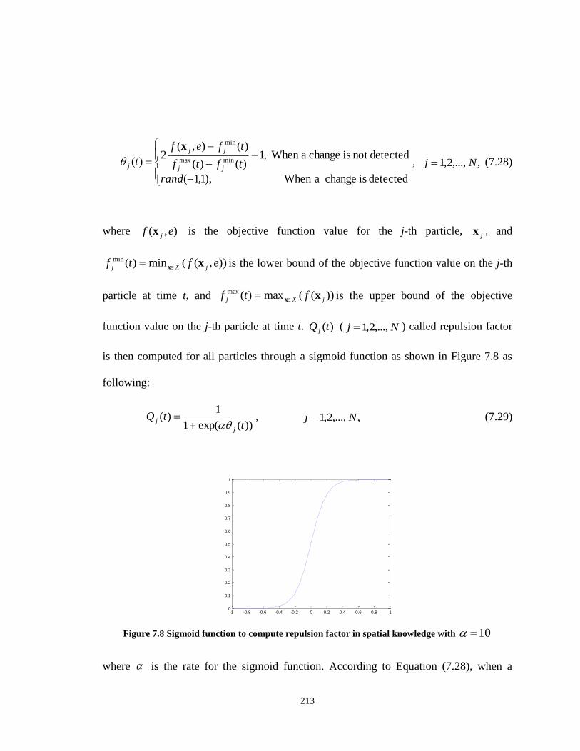
213

detected is change a When ),1,1(

detectednot is change a When ,1)()(

)(),(2

)( minmax

min

rand

tftf

tfef

tjj

jj

j

x

, ,,...,2,1 Nj (7.28)

where ),( ef jx is the objective function value for the j-th particle, jx , and

)),((min)(min eftf jXj xx is the lower bound of the objective function value on the j-th

particle at time t, and ))((max)(max

jXj ftf xx is the upper bound of the objective

function value on the j-th particle at time t. )(tQ j ( Nj ,...,2,1 ) called repulsion factor

is then computed for all particles through a sigmoid function as shown in Figure 7.8 as

following:

))(exp(1

1)(

ttQ

j

j

, ,,...,2,1 Nj (7.29)

Figure 7.8 Sigmoid function to compute repulsion factor in spatial knowledge with 10

where is the rate for the sigmoid function. According to Equation (7.28), when a

-1 -0.8 -0.6 -0.4 -0.2 0 0.2 0.4 0.6 0.8 10

0.1

0.2

0.3

0.4

0.5

0.6

0.7

0.8

0.9

1

214

change has not taken place in the environment, )(tj gets a value closer to –1 as its

objective function, ),( ef jx gets smaller, and closer to 1 as ),( ef jx gets larger. The

sigmoid transformation of Equation (7.29) will then compute the repulsion factor, )(tQ j

such that for the better half of the particles’ population, there is no or very small

repulsion factor and for the other half of the population space, the repulsion factor will be

close to 1 (e.g., for the best particle in the population space, 0)( tQi ). Hence during the

flight of particles of PSO, the better particles will not be repelled, so we do not lose

information of the better particles while the particles will be repelled from the worse

particles in the population space.

On the other hand, as soon as a change is detected, we do not want to force

particles to still be close to the best particles because the environment has changed and

they may not be any different from other particles. In this case, )(tj is statistically

assigned as a uniform random number between –1 and 1. It is then transformed through

the sigmoid function to compute )(tQ j . Statistically speaking, due to the performance of

the sigmoid function, a random half of the particles will be assigned a value close to zero

as repulsion factor, and the other half of the half will be assigned a value of 1. Although

this process avoids particles from being stuck near optimum point, but it also helps

preserve part of the evolutionary information stored in the search process and not

completely forget all the evolutionary data and re-start fresh. This mechanism helps to re-

diversify the search space quickly right after the change in the dynamic landscape is

215

detected and helps the algorithm with a jump start.

The spatial knowledge is updated at every iteration. After the PSO flight is

performed, the new positions of the particles will be evaluated using the objective

functions, and then the new spatial knowledge will be computed. Spatial knowledge will

be used to compute the repulsion term in the the flight mechanism.


After belief space is updated, the correspondent knowledge should be used to

influence the flight of particles in PSO. We propose to use the knowledge in belief space

to select the personal best, swarm best, and global best for the PSO mechanism, and to

perform the repulsive diversity-based migration among swarms.

7.3.4.1 pbest Selection

In order to select the personal best, we use information in the temporal knowledge

section of the belief space. The best behaving behavior in the particle’s past history

should be selected as following:

))},(min()ˆ(),()ˆ(1),()ˆ({)( ttfttfNjtttpbest jjjjjji TTP x (7.30)

( Pi ,...,2,1 )

216

where )}(),...,2(),1({)( tt jjjj xxxP is the set of all past positions of the j-th particle in the

whole population, and )}(),...,2(),1({)( tffft jjjj T ( Nj ,...,2,1 ) is the objective values

for the past history of the j-th particle, both extracted from the temporal knowledge

section of the belief space.

7.3.4.2 sbest Selection

In order to select the swarm best particle, the situational knowledge is adopted.

The information stored in the situational knowledge section of the belief space is simply

copied into swarm best particles:

),(ˆ)( ttsbest ii x ,,...,2,1 Pi (7.31)

where P is the number of swarms and )(ˆ tix is the representative of the situational

knowledge of the belief space.

7.3.4.3 gbest Selection

We use the domain knowledge stored in the belief space to copy the latest and

current element of )(tg of Equation (7.12) as the )(tgbest .

7.3.4.4 Diversity based Migration Driven by Change

217

In order to perform repulsive change-driven diversity based migration, we use

information in the domain knowledge and normative knowledge sections of the belief

space. The information in the domain knowledge will be used to monitor the change in

the dynamic, while information in the normative knowledge will be adopted to do the

migration as a response to the detected change. The change has taken place if and only if

there is at least one such that:

}{ 0 , (7.32)

where is defined as:

}.))(()({}))(()({ tfttft Sfsgfg (7.33)

)(tfg , )(tg , )(tfs and )(tS are adopted from the domain knowledge of the belief space,

and . denotes the absolute value. The allowable change, 0 , is set to a predefined small

value. Notice that there is a difference between objective function in Equation (7.33), i.e.,

))(( tf g and ))(( tf S , with the objective function in Equations (7.14) and (7.16), i.e.,

))(( tgbestf and ))(ˆ( tf ix , this difference is due to the possible environmental changes.

To be more precise, ))(),(())(( tetgbestftf g , is the objective value for all gbest

values (all previous iterations, t , in domain knowledge) computed using the “current” e.

While ))(),(())(( tetgbestftgbestf is the objective value for all gbest values (all

previous iterations, t , in domain knowledge) computed under the environmental

218

parameter e, at the previous iteration, t .Therefore any difference that appears in

Equation (7.33) should be due to the differences between the environmental parameter at

the current iteration, )(te , and the previous time, )( te .

When the change is detected, as the response to the change, we have to quickly

re-diversify because the previous optimum solutions are no longer valid for the new

environment. This response is performed using a repulsive diversity based migration

through the information in the normative knowledge of the belief space. As soon as the

change is detected, the data from the normative knowledge will be adopted to exchange

information among swarms. Each swarm accepts the sending list S from other swarm

and will replace it with its own replacement list, R (Both S andR are extracted from

the normative knowledge). This information exchange among swarms happens in a ring

sequential order between each pair of swarms.

7.4 Experimental Study

In this section the performance of the proposed cultural-based dynamic particle

swarm optimization is evaluated against those of the state-of-the-art dynamic particle

swarm optimization (DPSO) heuristics.

219

7.4.1 Benchmark Test Problems

Six test functions as benchmark problems have been used to test the ability of the

proposed cultural-based DPSO as following: MP1 (moving cone peaks benchmark

problem) is a maximization problem which has components as moving competing cones

with independently varying height, width and location [166]. DF2 (time-varying

Gaussian peaks problem) is a maximization problem that adopts independently varying-

dimensional Gaussian peaks. Each peak’s amplitude, center, and variance can be varied

independently [167]. DF3 is a minimization problem as moving parabola with linear

translation in change [168-169]. DF4 is also a minimization problem of moving parabola

but with random dynamics [168-169]. DF5 is a minimization problem of moving

parabola with circular dynamic [168-169] and finally DF6 (oscillating peaks function) is

a maximization problem that has been used in [170]. It has two landscapes with ten peaks

each. The parameters of each peak can independently vary. The detailed formulation of

these benchmark test functions are presented in Appendix C for reference.

For the simulations here, benchmark problems have the following parameter

setting wherever applies, unless stated otherwise: number of peaks is set as default value

of 10, every 5,000 evaluations the change takes place. The peak shape is cone (for MP1),

Gaussian (for DF2), parabola (for DF3, DF4, and DF5), and bell curve (for DF6). Default

decision space dimension is 5. Each decision variable is limited between 0 and 100. The

height and width severity are set as 7 and 1 respectively. The height peak is limited

220

between 30 and 70. The width peak is also limited between 1 and 12. Finally, the peak

shift length is set as 1.

7.4.2 Comparison Algorithms

The proposed algorithm has been compared against other state-of-the-art dynamic

particle swarm optimization paradigms that are adopted to solve DOPs. These algorithms

include DPSO [44], hybrid DPSO (h-DPSO) [92], modified DPSO (m-DPSO) [94] and

speciation based DPSO (s-DPSO) [96]. DPSO [44] is a regular particle swarm

optimization that adopts a simple strategy with a small perturbation, the initialization of

the swarm can start from old population, while with large perturbation, it does re-

initialize and then compare the results with the old swarm and select the best one. The

selected parameters are given in Table 7.1. For the moment of inertia, as suggested in

[44], a uniform random number with average of 0.75 is selected. In h-DPSO [92] a

dynamic macro-mutation operator plays the role of maintaining diversity throughout the

search process. The mutation is for every coordinate of each particle. The mutation will

take place with a probability within the minimum and maximum value given in Table 7.1

as suggested in [92] and possess its highest value when the change occurs in the dynamic

landscape and gradually decreases till the next change takes place. The swarm size and

neighborhood radius size are also given in this table as suggested in the literature [92].

The next algorithm is m-DPSO [94] the changed local optimum and global optimum are

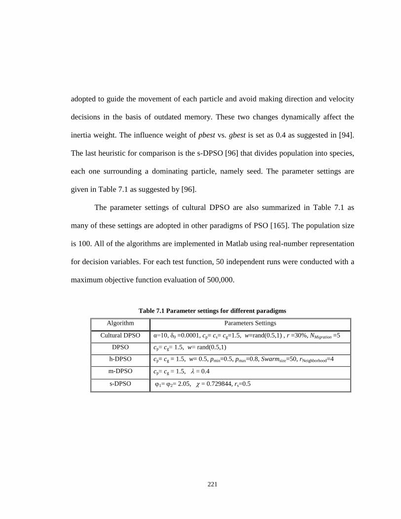
221

adopted to guide the movement of each particle and avoid making direction and velocity

decisions in the basis of outdated memory. These two changes dynamically affect the

inertia weight. The influence weight of pbest vs. gbest is set as 0.4 as suggested in [94].

The last heuristic for comparison is the s-DPSO [96] that divides population into species,

each one surrounding a dominating particle, namely seed. The parameter settings are

given in Table 7.1 as suggested by [96].

The parameter settings of cultural DPSO are also summarized in Table 7.1 as

many of these settings are adopted in other paradigms of PSO [165]. The population size

is 100. All of the algorithms are implemented in Matlab using real-number representation

for decision variables. For each test function, 50 independent runs were conducted with a

maximum objective function evaluation of 500,000.

Table 7.1 Parameter settings for different paradigms

Algorithm Parameters Settings

Cultural DPSO α=10, δ0 =0.0001, cp= cs= cg=1.5, w=rand(0.5,1) , r =30%, NMigration =5

DPSO cp= cg= 1.5, w= rand(0.5,1)

h-DPSO cp= cg = 1.5, w= 0.5, pmin=0.5, pmax=0.8, Swarmsize=50, rNeighborhood=4

m-DPSO cp= cg = 1.5, = 0.4

s-DPSO 1= 2= 2.05, = 0.729844, rs=0.5

222

7.4.3 Comparison Measure

To quantify the performance of the proposed paradigm, the offline error variation

(OEV) index,offlinee , defined as the average of the error between the true optimal fitness

and the best fitness at each evaluation [171] is used:

,)(1

1

T

i

i

BestTrueoffline ffT

e (7.34)

where i is the evaluation counter, T is the total number of evaluations, Truef is the true

optimum solution updated after a change occurs, and i

Bestf is the best individual out of the

evaluations starting from the last occurrence of change until the current evaluation. For

perfect tracking of change the offline error variation should be zero.

7.4.4 Simulation Results

The number of evaluations computed as the product of the population size and the

current iteration is used as the counter for comparing the paradigms against each other.

Table 7.2 compares the performance of the proposed cultural DPSO with selected state-

of-the-art DPSOs on test problem MP1 as a function of iterations elapsed between

changes, peak numbers and decision space dimensions, respectively. Figures (7.9) to

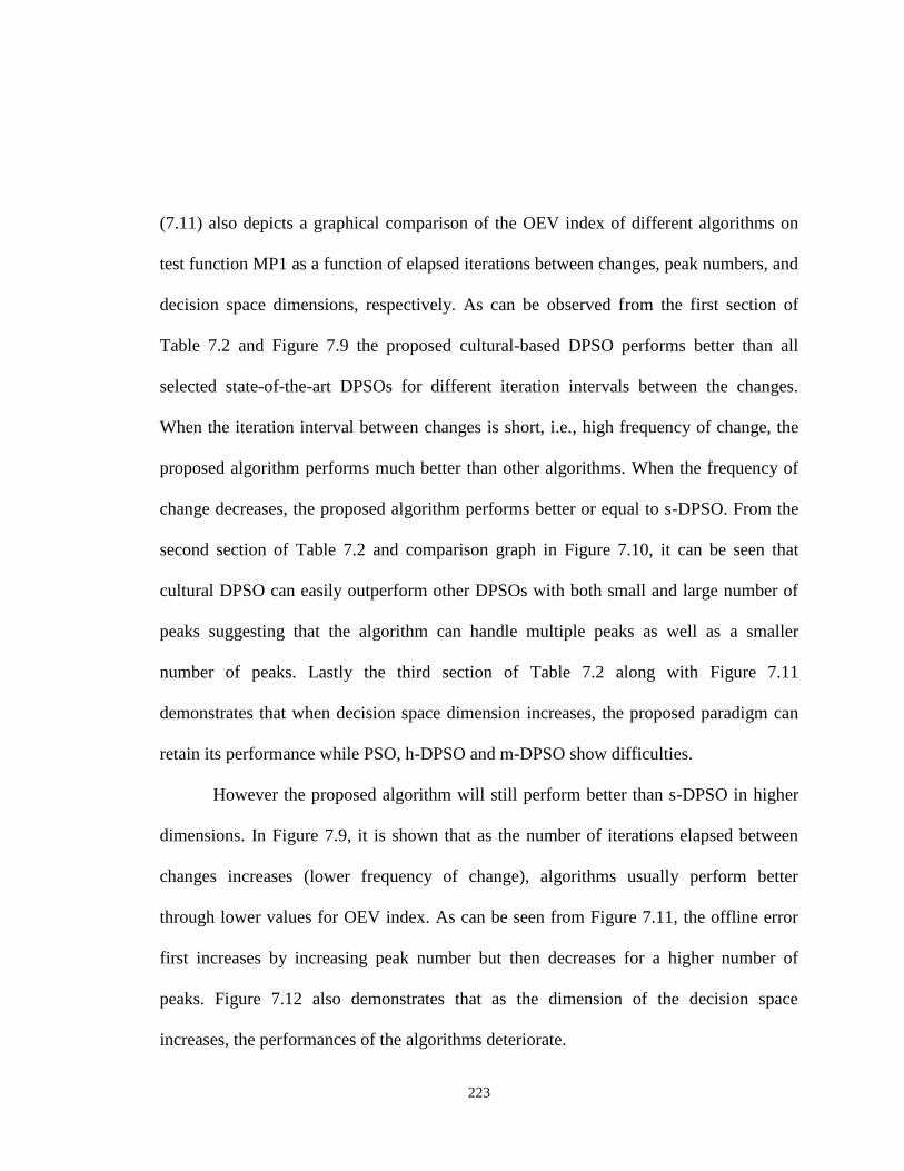
223

(7.11) also depicts a graphical comparison of the OEV index of different algorithms on

test function MP1 as a function of elapsed iterations between changes, peak numbers, and

decision space dimensions, respectively. As can be observed from the first section of

Table 7.2 and Figure 7.9 the proposed cultural-based DPSO performs better than all

selected state-of-the-art DPSOs for different iteration intervals between the changes.

When the iteration interval between changes is short, i.e., high frequency of change, the

proposed algorithm performs much better than other algorithms. When the frequency of

change decreases, the proposed algorithm performs better or equal to s-DPSO. From the

second section of Table 7.2 and comparison graph in Figure 7.10, it can be seen that

cultural DPSO can easily outperform other DPSOs with both small and large number of

peaks suggesting that the algorithm can handle multiple peaks as well as a smaller

number of peaks. Lastly the third section of Table 7.2 along with Figure 7.11

demonstrates that when decision space dimension increases, the proposed paradigm can

retain its performance while PSO, h-DPSO and m-DPSO show difficulties.

However the proposed algorithm will still perform better than s-DPSO in higher

dimensions. In Figure 7.9, it is shown that as the number of iterations elapsed between

changes increases (lower frequency of change), algorithms usually perform better

through lower values for OEV index. As can be seen from Figure 7.11, the offline error

first increases by increasing peak number but then decreases for a higher number of

peaks. Figure 7.12 also demonstrates that as the dimension of the decision space

increases, the performances of the algorithms deteriorate.

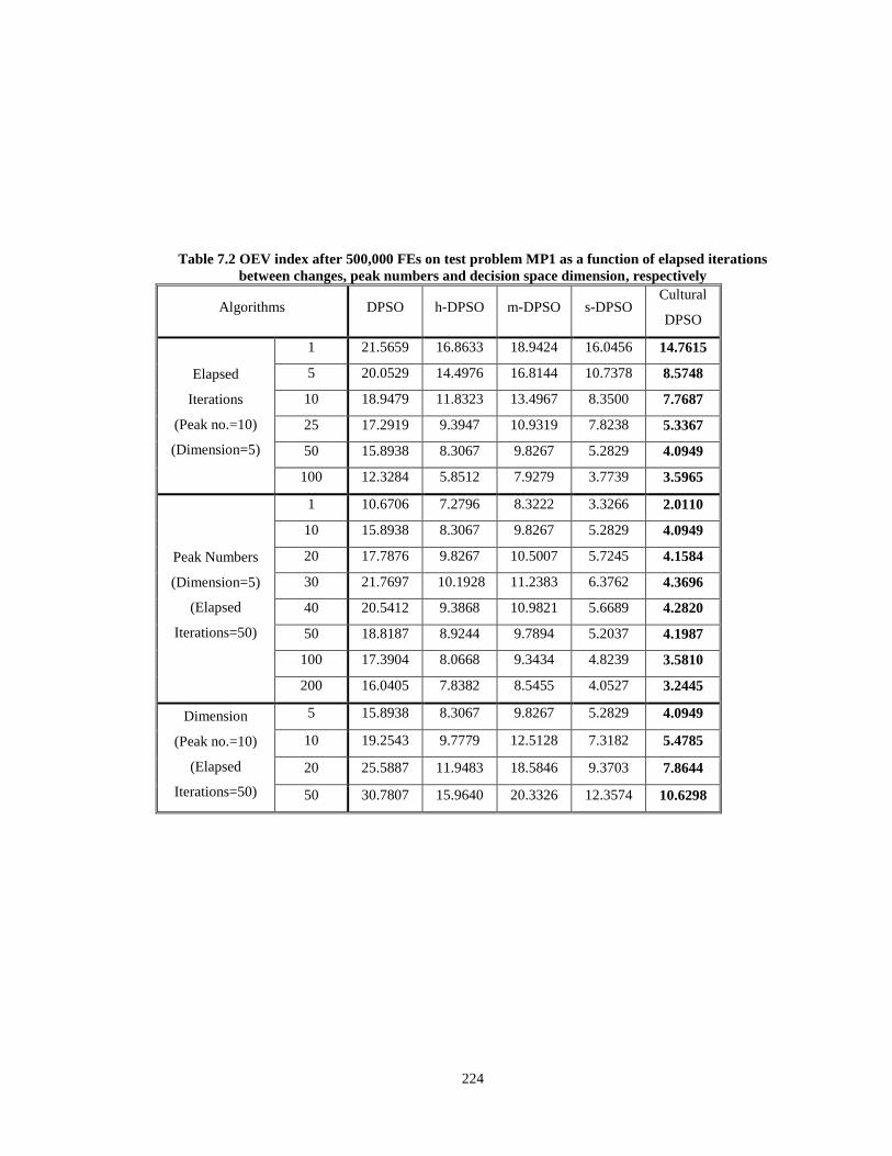
224

Table 7.2 OEV index after 500,000 FEs on test problem MP1 as a function of elapsed iterations

between changes, peak numbers and decision space dimension, respectively

Algorithms DPSO h-DPSO m-DPSO s-DPSO Cultural

DPSO

Elapsed

Iterations

(Peak no.=10)

(Dimension=5)

1 21.5659 16.8633 18.9424 16.0456 14.7615

5 20.0529 14.4976 16.8144 10.7378 8.5748

10 18.9479 11.8323 13.4967 8.3500 7.7687

25 17.2919 9.3947 10.9319 7.8238 5.3367

50 15.8938 8.3067 9.8267 5.2829 4.0949

100 12.3284 5.8512 7.9279 3.7739 3.5965

Peak Numbers

(Dimension=5)

(Elapsed

Iterations=50)

1 10.6706 7.2796 8.3222 3.3266 2.0110

10 15.8938 8.3067 9.8267 5.2829 4.0949

20 17.7876 9.8267 10.5007 5.7245 4.1584

30 21.7697 10.1928 11.2383 6.3762 4.3696

40 20.5412 9.3868 10.9821 5.6689 4.2820

50 18.8187 8.9244 9.7894 5.2037 4.1987

100 17.3904 8.0668 9.3434 4.8239 3.5810

200 16.0405 7.8382 8.5455 4.0527 3.2445

Dimension

(Peak no.=10)

(Elapsed

Iterations=50)

5 15.8938 8.3067 9.8267 5.2829 4.0949

10 19.2543 9.7779 12.5128 7.3182 5.4785

20 25.5887 11.9483 18.5846 9.3703 7.8644

50 30.7807 15.9640 20.3326 12.3574 10.6298

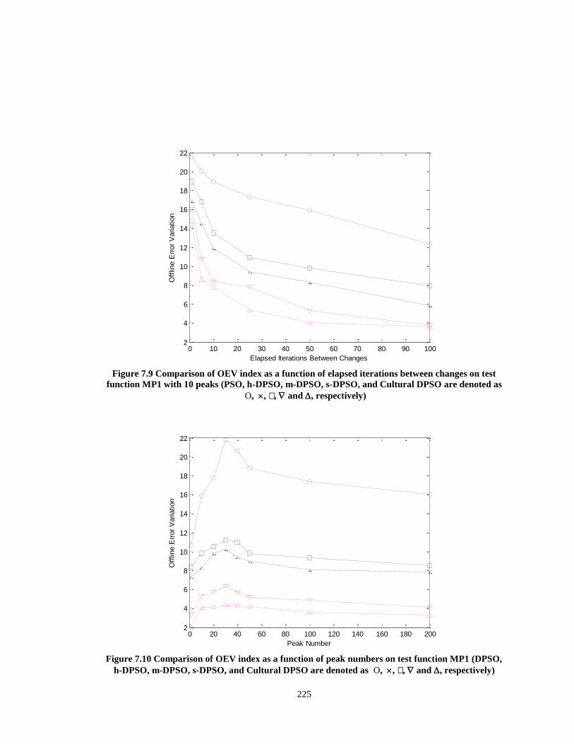
225

Figure 7.9 Comparison of OEV index as a function of elapsed iterations between changes on test

function MP1 with 10 peaks (PSO, h-DPSO, m-DPSO, s-DPSO, and Cultural DPSO are denoted as

O, , , and , respectively)

Figure 7.10 Comparison of OEV index as a function of peak numbers on test function MP1 (DPSO,

h-DPSO, m-DPSO, s-DPSO, and Cultural DPSO are denoted as O, , , and , respectively)

0 10 20 30 40 50 60 70 80 90 1002

4

6

8

10

12

14

16

18

20

22

Elapsed Iterations Between Changes

Off

line E

rror

Variation

0 20 40 60 80 100 120 140 160 180 2002

4

6

8

10

12

14

16

18

20

22

Peak Number

Off

line E

rror

Variation

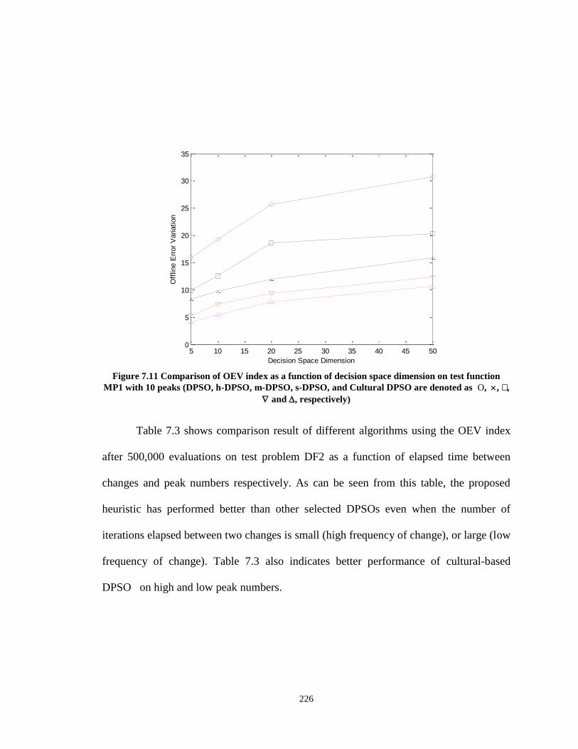
226

Figure 7.11 Comparison of OEV index as a function of decision space dimension on test function

MP1 with 10 peaks (DPSO, h-DPSO, m-DPSO, s-DPSO, and Cultural DPSO are denoted as O, , ,

and , respectively)

Table 7.3 shows comparison result of different algorithms using the OEV index

after 500,000 evaluations on test problem DF2 as a function of elapsed time between

changes and peak numbers respectively. As can be seen from this table, the proposed

heuristic has performed better than other selected DPSOs even when the number of

iterations elapsed between two changes is small (high frequency of change), or large (low

frequency of change). Table 7.3 also indicates better performance of cultural-based

DPSO on high and low peak numbers.

5 10 15 20 25 30 35 40 45 500

5

10

15

20

25

30

35

Decision Space Dimension

Off

line E

rror

Variation

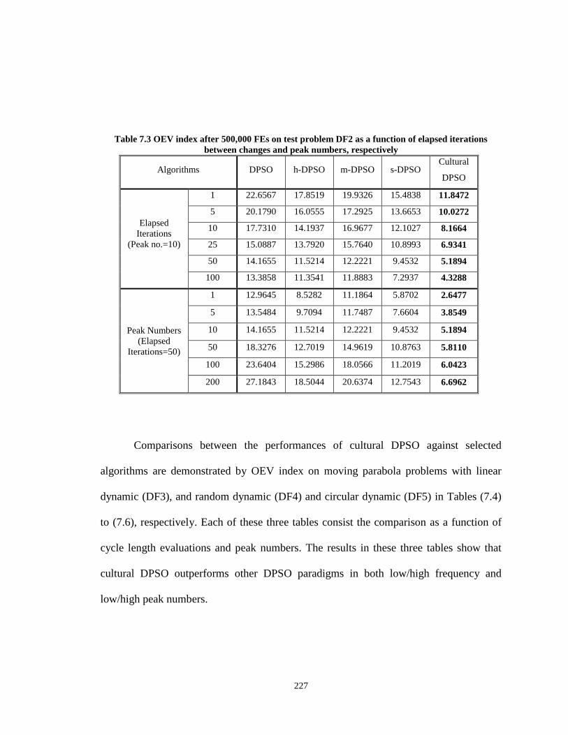
227

Table 7.3 OEV index after 500,000 FEs on test problem DF2 as a function of elapsed iterations

between changes and peak numbers, respectively


DPSO

Elapsed

Iterations

(Peak no.=10)

1 22.6567 17.8519 19.9326 15.4838 11.8472

5 20.1790 16.0555 17.2925 13.6653 10.0272

10 17.7310 14.1937 16.9677 12.1027 8.1664

25 15.0887 13.7920 15.7640 10.8993 6.9341

50 14.1655 11.5214 12.2221 9.4532 5.1894

100 13.3858 11.3541 11.8883 7.2937 4.3288

Peak Numbers

(Elapsed

Iterations=50)

1 12.9645 8.5282 11.1864 5.8702 2.6477

5 13.5484 9.7094 11.7487 7.6604 3.8549

10 14.1655 11.5214 12.2221 9.4532 5.1894

50 18.3276 12.7019 14.9619 10.8763 5.8110

100 23.6404 15.2986 18.0566 11.2019 6.0423

200 27.1843 18.5044 20.6374 12.7543 6.6962

Comparisons between the performances of cultural DPSO against selected

algorithms are demonstrated by OEV index on moving parabola problems with linear

dynamic (DF3), and random dynamic (DF4) and circular dynamic (DF5) in Tables (7.4)

to (7.6), respectively. Each of these three tables consist the comparison as a function of

cycle length evaluations and peak numbers. The results in these three tables show that

cultural DPSO outperforms other DPSO paradigms in both low/high frequency and

low/high peak numbers.

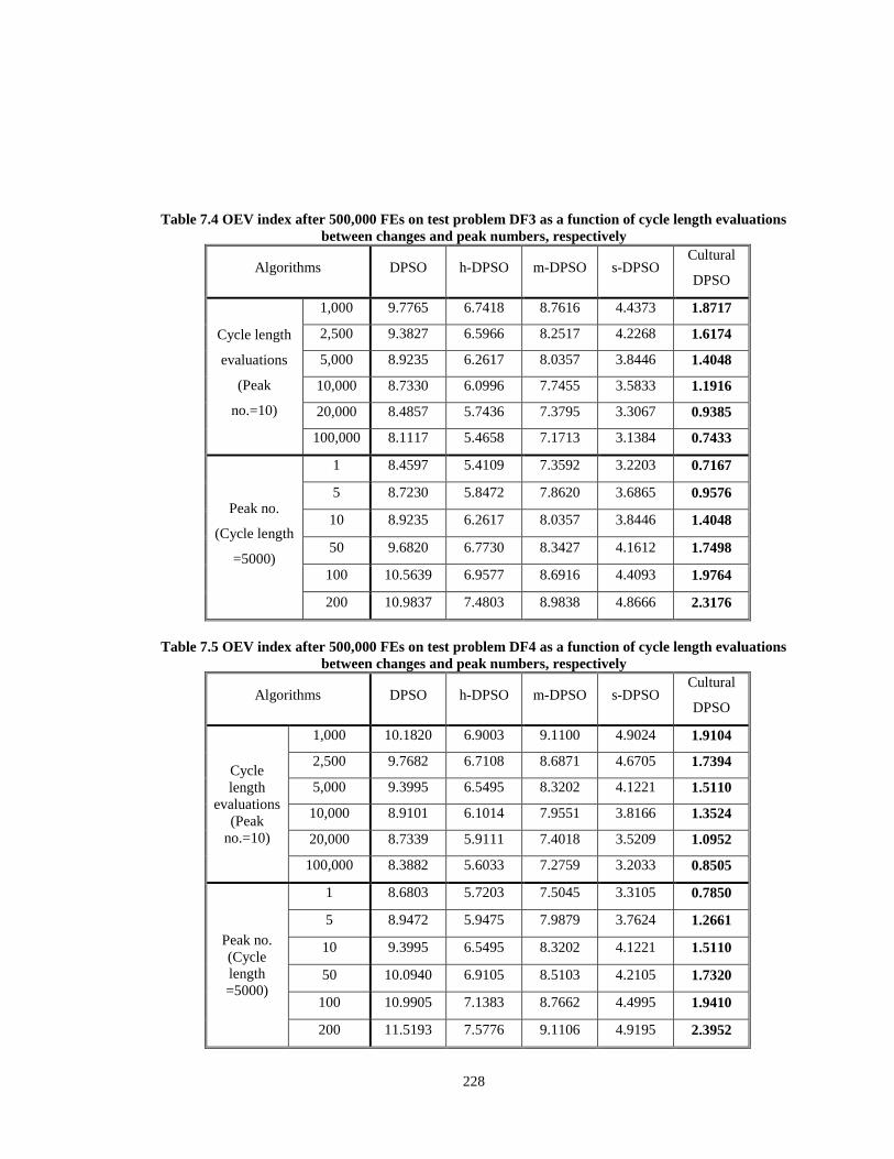
228

Table 7.4 OEV index after 500,000 FEs on test problem DF3 as a function of cycle length evaluations



DPSO

Cycle length

evaluations

(Peak

no.=10)

1,000 9.7765 6.7418 8.7616 4.4373 1.8717

2,500 9.3827 6.5966 8.2517 4.2268 1.6174

5,000 8.9235 6.2617 8.0357 3.8446 1.4048

10,000 8.7330 6.0996 7.7455 3.5833 1.1916

20,000 8.4857 5.7436 7.3795 3.3067 0.9385

100,000 8.1117 5.4658 7.1713 3.1384 0.7433

Peak no.

(Cycle length

=5000)

1 8.4597 5.4109 7.3592 3.2203 0.7167

5 8.7230 5.8472 7.8620 3.6865 0.9576

10 8.9235 6.2617 8.0357 3.8446 1.4048

50 9.6820 6.7730 8.3427 4.1612 1.7498

100 10.5639 6.9577 8.6916 4.4093 1.9764

200 10.9837 7.4803 8.9838 4.8666 2.3176




DPSO

Cycle

length

evaluations

(Peak

no.=10)

1,000 10.1820 6.9003 9.1100 4.9024 1.9104

2,500 9.7682 6.7108 8.6871 4.6705 1.7394

5,000 9.3995 6.5495 8.3202 4.1221 1.5110

10,000 8.9101 6.1014 7.9551 3.8166 1.3524

20,000 8.7339 5.9111 7.4018 3.5209 1.0952

100,000 8.3882 5.6033 7.2759 3.2033 0.8505

Peak no.

(Cycle

length

=5000)

1 8.6803 5.7203 7.5045 3.3105 0.7850

5 8.9472 5.9475 7.9879 3.7624 1.2661

10 9.3995 6.5495 8.3202 4.1221 1.5110

50 10.0940 6.9105 8.5103 4.2105 1.7320

100 10.9905 7.1383 8.7662 4.4995 1.9410

200 11.5193 7.5776 9.1106 4.9195 2.3952

229




DPSO

Cycle

length

evaluations

(Peak

no.=10)

1,000 10.3495 7.2870 9.4110 5.1551 1.9840

2,500 9.9478 6.9485 8.8660 4.8400 1.7910

5,000 9.5980 6.8778 8.5229 4.3481 1.6258

10,000 9.1336 6.3227 8.1593 3.9330 1.4817

20,000 8.9105 6.1005 7.7206 3.6484 1.2155

100,000 8.5119 5.7490 7.4605 3.3710 0.9750

Peak no.

(Cycle

length

=5000)

1 8.9209 5.8103 7.7101 3.5103 0.8929

5 9.1332 6.1854 8.1690 3.9004 1.3820

10 9.5980 6.8778 8.5229 4.3481 1.6258

50 10.2059 7.1100 8.6202 4.4820 1.8720

100 11.2449 7.3665 8.9110 4.6114 2.0973

200 11.7101 7.6505 9.5339 5.1776 2.5191

Test function DF6 has two landscapes with ten peaks as it has been used in [170].

The parameters of each peak can be varied independently. In Table 7.7, the performance

of selected algorithms is compared for different cycle lengths. As can be observed from

the table, the cultural DPSO shows better performance both in lower and higher

frequencies of change compared to DPSO, h-DPSO and m-DPSO, while its performance

is equal to or less than s-PSO in high frequency of change and equal to or better than s-

PSO in low frequency of changes. For better quantitative comparison of the algorithms

over all benchmark problems, the Mann–Whitney rank sum test has been conducted to

examine the significance of the difference between the algorithms [132]. In Table 7.8, the

p-values with respect to the alternative hypothesis (for p-values less than α=0.5) for each

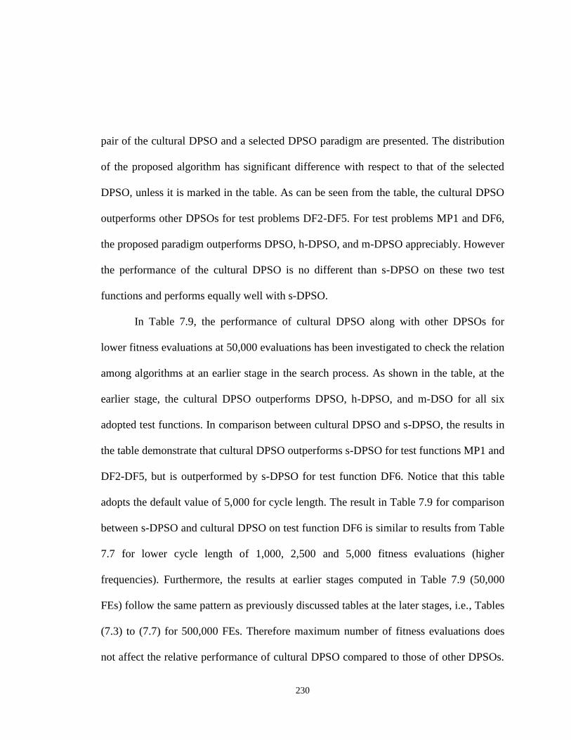
230

pair of the cultural DPSO and a selected DPSO paradigm are presented. The distribution

of the proposed algorithm has significant difference with respect to that of the selected

DPSO, unless it is marked in the table. As can be seen from the table, the cultural DPSO

outperforms other DPSOs for test problems DF2-DF5. For test problems MP1 and DF6,

the proposed paradigm outperforms DPSO, h-DPSO, and m-DPSO appreciably. However

the performance of the cultural DPSO is no different than s-DPSO on these two test

functions and performs equally well with s-DPSO.

In Table 7.9, the performance of cultural DPSO along with other DPSOs for

lower fitness evaluations at 50,000 evaluations has been investigated to check the relation

among algorithms at an earlier stage in the search process. As shown in the table, at the

earlier stage, the cultural DPSO outperforms DPSO, h-DPSO, and m-DSO for all six

adopted test functions. In comparison between cultural DPSO and s-DPSO, the results in

the table demonstrate that cultural DPSO outperforms s-DPSO for test functions MP1 and

DF2-DF5, but is outperformed by s-DPSO for test function DF6. Notice that this table

adopts the default value of 5,000 for cycle length. The result in Table 7.9 for comparison

between s-DPSO and cultural DPSO on test function DF6 is similar to results from Table

7.7 for lower cycle length of 1,000, 2,500 and 5,000 fitness evaluations (higher

frequencies). Furthermore, the results at earlier stages computed in Table 7.9 (50,000

FEs) follow the same pattern as previously discussed tables at the later stages, i.e., Tables

(7.3) to (7.7) for 500,000 FEs. Therefore maximum number of fitness evaluations does

not affect the relative performance of cultural DPSO compared to those of other DPSOs.

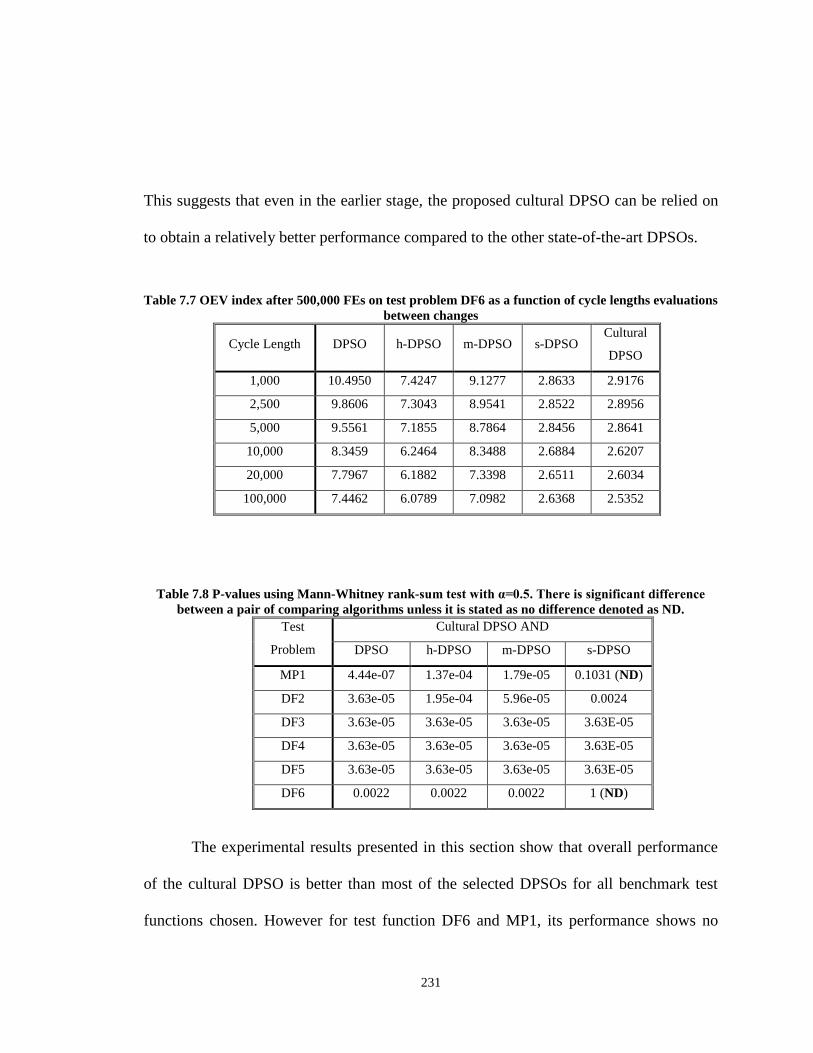
231

This suggests that even in the earlier stage, the proposed cultural DPSO can be relied on

to obtain a relatively better performance compared to the other state-of-the-art DPSOs.

Table 7.7 OEV index after 500,000 FEs on test problem DF6 as a function of cycle lengths evaluations

between changes

Cycle Length DPSO h-DPSO m-DPSO s-DPSO Cultural

DPSO

1,000 10.4950 7.4247 9.1277 2.8633 2.9176

2,500 9.8606 7.3043 8.9541 2.8522 2.8956

5,000 9.5561 7.1855 8.7864 2.8456 2.8641

10,000 8.3459 6.2464 8.3488 2.6884 2.6207

20,000 7.7967 6.1882 7.3398 2.6511 2.6034

100,000 7.4462 6.0789 7.0982 2.6368 2.5352

Table 7.8 P-values using Mann-Whitney rank-sum test with α=0.5. There is significant difference

between a pair of comparing algorithms unless it is stated as no difference denoted as ND.

Test

Problem

Cultural DPSO AND

DPSO h-DPSO m-DPSO s-DPSO

MP1 4.44e-07 1.37e-04 1.79e-05 0.1031 (ND)

DF2 3.63e-05 1.95e-04 5.96e-05 0.0024

DF3 3.63e-05 3.63e-05 3.63e-05 3.63E-05

DF4 3.63e-05 3.63e-05 3.63e-05 3.63E-05

DF5 3.63e-05 3.63e-05 3.63e-05 3.63E-05

DF6 0.0022 0.0022 0.0022 1 (ND)

The experimental results presented in this section show that overall performance

of the cultural DPSO is better than most of the selected DPSOs for all benchmark test

functions chosen. However for test function DF6 and MP1, its performance shows no

232

difference when compared to s-DPSO (both in earlier and later stages of search process).

However the proposed cultural DPSO still well outperforms s-DPSO on other four

benchmark test problems as shown by Mann-Whitney statistical tests. This suggests that

cultural algorithm with its abilities such as different sections of belief space prepares an

organized informational storage that will help the process of quick re-divergence and re-

convergence around new optimum points when a change happens in the dynamic of the

problem.

Table 7.9 OEV index after 50,000 FEs using default parameters


DPSO

MP1 16.9269 9.4858 10.6862 4.9268 4.3686

DF2 15.1176 12.8552 13.9242 10.4435 5.4236

DF3 9.6942 7.4026 9.6903 4.9584 1.6409

DF4 10.0439 7.1154 9.8032 5.9512 1.6814

DF5 10.7485 7.3807 9.9352 5.7724 1.7366

DF6 10.9565 8.2904 9.6078 2.8526 2.9067

7.5 Discussions

In this study, the cultural-based dynamic particle swarm optimization has been

proposed to solve DOP problems. This novel heuristic is built upon a cultural framework

that consist two sections, a multiple swarm PSO as the population space and a belief

space including five sections: situational knowledge, temporal knowledge, domain

233

knowledge, normative knowledge, and spatial knowledge. The required information are

categorized properly in the belief space in such a manner that can be easily accessed to

move toward the optimum solution in the population space, and to monitor and detect any

possible changes in the environment, also to respond quickly to the occurred changes by

a repulsive diversity-promoted migration. When particles share their information through

migration process, they will be able to quickly re-diversify and move efficiently towards

new optimum by re-converging around it. The cultural information stored in the belief

space will assist the population space in selecting the leading particles in the PSO flight.

The flight mechanism follows a three level movement along with a repulsive term that is

effective when a change has taken place. The three-level flight happens in the personal

level, swarm level, and global level for which all leading particles will be assessed

through the information extracted from different sections of the belief space. The

particles will also repel each other the most, when a change has happened through a

sigmoid repulsion factor. This phenomenon is repeatedly observed in the psychosocial

studies as repulsion in interpersonal relationship among individuals generating new

cultural opportunities through cultural divergence.

The novel cultural-based dynamic PSO is evaluated against some selected state-

of-the-art evolutionary algorithm and particle swarm based heuristics on different

benchmark dynamic test functions. Comparison study through experimental results show

that the novel cultural-based dynamic PSO outperforms the selected state-of-the-art

dynamic PSOs in almost all benchmark test functions suggesting that the organized and

234

categorized cultural information stored in belief space assist in better performing the

search process under dynamic environment. The information extracted from belief space

drives the repulsive divergence-promoted migration to quickly re-diversify the particles

in the search space after a change takes place in the dynamic landscape and re-converge

them through a modified three-level flight mechanism around new optimum. As a future

work, it is suggested that the personal, swarm and global acceleration will not be a fixed

value as it is in this study, but follow a dynamic behavior and adapt based upon the

particle’s or swarm’s needs in the spatial space of the belief space as it can be observed

how dynamic acceleration can improve the result of PSO convergence [140-141].

235

CHAPTER VIII

CONCLUSION

In this dissertation, several innovative heuristics using sociologically inspired

concepts such as society and civilization, migration, communication, culture, swarms and

beliefs have been proposed to solve engineering single objective optimization, multi

objective optimization, constrained optimization and dynamic optimization problems.

A politically inspired measure called liberty rate has been introduced to facilitate

the optimization process in social-based optimization algorithm. The simulation results

show the performance improvement attained by accumulating the liberty rate into the

original heuristics. The second modification on social-based optimization algorithm is to

collect information from all individuals for migration purposes.

A diversity-based migration process among swarms in particle swarm

optimization has also been proposed to solve multimodal optimization problems. The

proposed PSO flight mechanism includes three levels which in turn also diversify its

search ability. In the lowest level, particles follow the best behaving particle in their own

swarm; in next level, particles follow the best performing particle in the neighboring

swarms, and finally in the highest level, particles track the whole population’s best

236

behaving particle. Adopting a two-way communication among each pair of swarms, the

particles do not fall prematurely stuck in the local optima. The exchanged particles are

selected according to the location of the particles based on a diversity strategy and their

correspondence objective values. Furthermore, the PSO was modified using a new

neighborhood term that helps the neighboring swarms share the common interest

information. The neighborhood for each swarm is found using an unsupervised algorithm

according to the inter-swarm distances between representatives of each pair of swarms.

Simulation results on multimodal problems demonstrate that the proposed algorithm N-

DMPSO shows a great performance compared to DMPSO and two versions of distributed

genetic algorithm that share similar basis with the proposed algorithm. The DMPSO

showed competitive results compared to DGAs. The N-DMPSO showed better

performance compared to DMPSO, assuming that sharing information in the

neighborhood of swarms helps to escape from local optima and locate the global

optimum. However N-DMPSO and DMPSO both are dependent to the rate of

information exchange.

A novel heuristics of cultural MOPSO has also been proposed to adjust flight

parameters such as personal acceleration, global acceleration and momentum. Cultural

algorithm provides the required groundwork enabling us to employ the information

stored in different sections of belief space efficiently and effectively. Using the

knowledge stored in various parts of belief space such as normative, situational, and

topographical knowledge, cultural MOPSO shows promising results when compared to

237

some well-regarded MOPSOs. The comparison study based upon the hypervolume

indicator and additive binary epsilon indicator show that cultural MOPSO provides better

solution when compared on different hard benchmark test functions with high dimension

and complexity. Indeed cultural MOPSO outperforms all selected well-regarded

MOPSOs, except in one test function there is no difference between cultural MOPSO and

another MOPSO. Consequently cultural MOPSO is significantly better than most

MOPSOs and weakly dominates all of the selected MOPSOs.

Further comprehensive investigation of the cultural MOPSO demonstrates its

robustness with respect to the algorithm’s tuning parameters. In an extensive sensitivity

analysis, the final Pareto fronts of any pair of algorithms are compared when one

parameter is changed. Using additive binary epsilon indicator, the analysis demonstrate

an almost-robust algorithm when nine different parameters of the algorithm are varied,

i.e., about 95% of the tests indicates no change of results by tuning the parameters.

Additionally, a new cultural constrained particle swarm optimization has been

proposed to solve constrained optimization problems. The heuristics incorporates

information of objective function and constraints violation, to construct a cultural

framework consisting two sections: a multiple swarm PSO with the ability of inter-swarm

communication as population space and a belief space including four parts, normative

knowledge, spatial knowledge, situational knowledge, and temporal knowledge. Every

particle will fly through a three-level flight and then particles divide into several swarms

and inter-swarm communication takes place to exchange the information. The cultural

238

CPSO is evaluated against 10 state-of-the-art constrained optimization paradigms on 24

difficult benchmark test problems. The simulation results show that cultural CPSO has

the average feasible rate of 95.83% on 24 benchmark problems that places it as top

performing algorithm along with DMS-PSO [149], _DE [150] and SaDE [157]. It also

indicates that the proposed cultural CPSO has the average success rate of 90.00% on all

benchmark problems placing it at the third best performing algorithm after _DE and

PCX [155] with 91.67% and 90.17% of success rate, respectively. Overall, cultural CPSO

is able to perform well competing with other well-performing algorithms in the field in

terms of feasible rate and success rate.

Furthermore, the novel cultural-based dynamic particle swarm optimization has

been proposed in order to solve DOP problems. Built upon a cultural framework

consisting a multiple swarm PSO as the population space and a belief space including

five sections, situational knowledge, temporal knowledge, domain knowledge, normative

knowledge, and spatial knowledge, the cultural-based DPSO categorizes effectively the

required information in the belief space in such a manner that can be easily accessed.

The information extracted from the belief space assists on moving toward the

optimum solution in the population space, and to detect any occurring changes in the

environment, also to respond quickly to the occurred changes by a repulsive diversity-

promoted migration. When particles share their information through migration process,

they will be able to quickly re-diversify and move efficiently towards new optimum by

re-converging around it. The cultural information stored in the belief space will assist the

239

population space in selecting the leading particles in the PSO flight. The flight

mechanism follows a three level movement along with a repulsive term that is most-

affective when a change has taken place. The three-level flight happens in the personal

level, swarm level, and global level for which all leading particles will be assessed

through the information extracted from different sections of the belief space. The

particles will also repel each other the most, when a change has happened through a

sigmoid repulsion formulation.

The cultural-based dynamic PSO has also been evaluated against some selected

state-of-the-art dynamic PSO heuristics on different benchmark dynamic test functions.

Comparison study demonstrates that the proposed cultural-based dynamic PSO performs

better or equally when compared with the selected state-of-the-art dynamic PSOs in all

benchmark test functions suggesting that the organized and categorized cultural

information stored in belief space assist in better performing the search process in

dynamic environment. The information extracted from belief space drives the repulsive

divergence-promoted migration to quickly re-diversify the particles in the search space

after a change takes place in the dynamic landscape and re-converge them through a

modified three-level flight mechanism around new optimum.

Overall, in this dissertation, cultural-based particle swarm optimization has been

proposed to solve different types of optimization problems ranging from a single

objective, multiobjective, constrained and finally dynamic optimization problems. The

incorporation of elements of culture through the well-organized belief space assists the

240

retrieving process of required information much easier. In all of these proposed

heuristics, the main structure of the algorithm follows an identical framework as far as

population space, acceptance function, and influence function and finally different

sections of belief space such as normative knowledge, situational knowledge, spatial

knowledge, temporal knowledge, and domain knowledge depending on the need of the

proposed paradigms. The flourishing performance of cultural-based PSO can be

understood due to its all-the-time monitoring and adjustment through the feedback

process from the population space, via acceptance function to belief space, and back to

the population space via the influence functions. This feedback fundamentally assists in

adjusting the optimum parameters for the entire system. The cultural PSO proposed here

has seen a great success when compared experimentally against other state-of-the-art

heuristics in different types of optimization problems, suggesting its further potential to

be developed and its potentially successful applications on developing optimization

algorithms for real-world problems.

241

BIBLIOGRAPHY

[1] J. Kennedy and R.C. Eberhart, “Particle swarm optimization,” In Proceedings of

the IEEE International Joint Conference on Neural Networks, Perth, Australia,

pp. 1942-1948, 1995.

[2] M. Dorigo, V. Maniezzo and A. Colorni, “Ant system: optimization by a colony

of cooperating agents,” IEEE Transactions on Systems, Man, Cybernetics, Part B,

Vol. 26, pp. 29-41, 1996.

[3] R.G. Reynolds, “An introduction to cultural algorithms,” In Proceedings of the

3rd Annual Conference on Evolutionary Programming, River Edge, NJ, USA, pp.

131-139, 1994.

[4] R.K. Ursem, “Multinational evolutionary algorithm,” In Proceedings of the IEEE

Congress on Evolutionary Computation, Washington, DC, USA, pp. 1633-1640,

1999.

[5] T. Ray and K. M. Liew, “Society and civilization: an optimization algorithm

based on the simulation of social behavior,” IEEE Transactions on Evolutionary

Computation, Vol. 7, No. 4, pp. 386-396, 2003.

[6] P. Grosso, “Computer simulation of genetic adaptations: parallel subcomponent

interaction in a multilocus mode,” University of Michigan, Ann Arbor, MI, USA,

1985.

[7] C. Anderson and D.W. McShea, “Individual versus social complexity, with

particular reference to ant colonies,” Biological Review, Vol. 76, pp. 211-237,

2001.

[8] L.A. Sjaastad, “The costs and returns of human migration,” The Journal of

Political Economy, Vol. 70, No. 5, pp. 80-93, 1962.

[9] G. Bottomley, “From another place: migration and the politics of culture,”

Cambridge University Press, Cambridge, United Kingdom, 1992.

242

[10] T. Blackwell, J. Branke and X. Li, “Particle swarms for dynamic optimization

problems,” In: Swarm Intelligence: Introduction and Application, C. Blum and D.

Merkle (Editors), Natural Computing Series, pp. 193-217, 2008.

[11] J. Xu, P.B. Luh, F.B. White, E. Ni and K. Kasiviswanathan, “Power portfolio

optimization in deregulated electricity markets with risk management,” IEEE

Transaction on Power Systems, Vol. 21, pp. 145-158, 2006.

[12] Y. Jin and J. Branke, “Evolutionary optimization in uncertain environments – A

survey,” IEEE Transaction on Evolutionary Computation, Vol. 9, pp. 303-317,

2005.

[13] R.W. Morrison and K.A. deJong, “A test problem generator for nonstationary

environments,” In Proceedings of the IEEE Congress on Evolutionary

Computation, Washington, DC, USA, pp. 2047-2053, 1999.

[14] M.E. Rosenbaum, “The repulsion hypothesis: On the nondevelopment of

relationships,” Journal of Personality and Social Psychology, Vol. 51, No. 6, pp.

1156-1166, 1986.

[15] J. Berger and C. Heath, “Who drives divergence? Identity signaling, outgroup

dissimilarity, and the abandonment of cultural tastes,” Journal of Personality and

Social Psychology, Vol. 95, No. 3, pp. 593-607, 2008.

[16] J.H. Holland, “Adaptation in Natural and Artificial Systems,” MIT Press,

Cambridge, MA, USA, 1992.

[17] L. Davis, “Handbook of genetic algorithms,” Van Nostrand Reinhold, New York,

NY, USA, 1991.

[18] J. Denzinger and J. Kidney, “Improving migration by diversity,” In Proceedings

of the IEEE Congress on Evolutionary Computation, Canberra, Australia, pp.

700-707, 2003.

[19] F. Heppner and U. Grenander, “A stochastic nonlinear model for coordinated bird

flocks,” In S. Krasner, Ed., The Ubiquity of Chaos, AAAS Publications,

Washington, DC, USA, pp. 233-238, 1990.

243

[20] J.L. Deneubourg and S. Goss, “Collective patterns and decision-making,”

Ethology, Ecology & Evolution, Vol. 1, pp. 295-311, 1989.

[21] M.M. Millonas, “Swarms, phase transitions, and collective intelligence,” In C. G.

Langton, Ed., Artificial Life III. Addison Wesley, pp. 417-445, 1994.

[22] C.W. Reynolds, “Flocks, herds and schools: a distributed behavioral model,”

Computer Graphics, Vol. 21, No. 4, pp. 25-34, 1987.

[23] S. Akhtar, K. Tai and T. Ray, “A socio-behavioral simulation model for

engineering design optimization,” Engineering Optimization, Vol. 34, pp. 341-

354, 2002.

[24] R.K. Ursem, “When sharing fails,” In Proceedings of the IEEE Congress on

Evolutionary Computation, Seoul, South Korea, pp. 873-879, 2001.

[25] J.L. Deneubourg, J.M. Pasteels and J.C. Verhaeghe, “Probabilistic behavior in

ants: a strategy of errors?” Journal of Theoretical Biology, Vol. 105, pp. 259-271,

1983.

[26] S. Goss, R. Beckers, J.L. Deneubourg, S. Aron and J.M. Pasteels, “How trail

laying and trail following can solve foraging problems for ant colonies,”

Behavioral Mechanisms of Food Selection, Vol. G20, Berlin:Springer-Verlag,

1990.

[27] M. Dorigo and G. DiCaro, “Ant colony optimization: a new meta-heuristic,” In

Proceedings of the IEEE Congress on Evolutionary Computation, Washington,

DC, USA, pp. 1470-1477, 1999.

[28] L.M. Gambardella and M. Dorigo, “Solving symmetric and asymmetric TSPs by

ant colonies,” In Proceedings of the IEEE International Conference on

Evolutionary Computation, Nagoya, Japan, pp. 622-627, 1996.

[29] M. Dorigo and L.M. Gambardella, “Ant colony system: A cooperative learning

approach to the traveling salesman problem,” IEEE Transactions on Evolutionary

Computation, Vol. 1, pp. 53-66, 1997.

244

[30] V. Maniezzo and A. Colorni, “The ant system applied to the quadratic assignment

problem,” IEEE Transactions on Knowledge and Data Engineering, Vol. 11, pp.

769-778, 1999.

[31] G. DiCaro and M. Dorigo, “Mobile agents for adaptive routing,” In Proceedings

of the 31st Hawaii International Conference on Systems Sciences, Kohala Coast,

HI, USA, pp. 74-83, 1998.

[32] E. Sahin, T. H. Labella, V. Trianni, J. Deneubourg, P. Rasse, D. Floreano, L.

Gambardella, F. Mondada, S. Nolfi and M. Dorigo, “SWARM-BOT: pattern

formation in a swarm of self-assembling mobile robots,” In Proceedings of the

IEEE International Conference on Systems, Man and Cybernetics, Yasmine

Hammamet, Tunisia, pp. 145-150, 2002.

[33] R.C. Eberhart and J. Kennedy, “A new optimizer using particle swarm theory,” In

Proceedings of the IEEE 6th

International Symposium on Micro Machine and

Human Science, Nagoya, Japan, pp. 39-43, 1995.

[34] Y. Shi and R.C. Eberhart, “A modified particle swarm optimizer,” In Proceedings

of the IEEE Congress on Evolutionary Computation, Anchorage, AK, USA, pp.

69-73, 1998.

[35] J. Kennedy, “Bare bones particle swarms,” In Proceedings of the IEEE Swarm

Intelligence Symposium, Indianapolis, IN, USA, pp. 80-87, 2003.

[36] M. Clerc and J. Kennedy, “The particle swarm - explosion, stability, and

convergence in a multidimensional complex space,” IEEE Transactions on

Evolutionary Computation, Vol. 6, pp. 58-73, 2002.

[37] J. Kennedy and R. Mendes, “Population structure and particle swarm

performance,” In Proceedings of the IEEE Congress on Evolutionary

Computation, Honolulu, HI, USA, pp. 1671-1676, 2002.

[38] J. Kennedy and R. Mendes, “Neighborhood topologies in fully-informed and best-

of-neighborhood particle swarms,” IEEE Transactions on Systems, Man,

Cybernetics, Part C, Vol. 36, pp. 515-519, 2006.

245

[39] R. Mendes, J. Kennedy and J. Neves, “Watch thy neighbor or how the swarm can

learn from its environment,” In Proceedings of the IEEE Swarm Intelligence

Symposium, Indianapolis, IN, USA, pp. 88-94, 2003.

[40] J. Kennedy and R.C. Eberhart, “A discrete binary version of the particle swarm

algorithm,” In Proceedings of the IEEE International Conference on

Computational Cybernetics and Simulation, Orlando, FL, USA, pp. 4104-4108,

1997.

[41] J. Kennedy and W.M. Spears, “Matching algorithms to problems: an experimental

test of the particle swarm and some genetic algorithms on the multimodal problem

generator,” In Proceedings of the IEEE International Conference on Evolutionary

Computation, Anchorage, AK, USA, pp. 78-83, 1998.

[42] Y. Shi and R.C. Eberhart, “Empirical study of particle swarm optimization,” In


DC, USA, pp. 1945-1950, 1999.

[43] R.C. Eberhart and Y. Shi, “Comparing inertia weights and constriction factors in

particle swarm optimization,” In Proceedings of the IEEE Congress on

Evolutionary Computation, La Jolla, CA, USA, pp. 84-88, 2000.

[44] R.C. Eberhart and Y. Shi, “Tracking and optimizing dynamic systems with

particle swarms,” In Proceedings of the IEEE Congress on Evolutionary

Computation, Seoul, South Korea, pp. 94-100, 2001.

[45] X. Hu, R.C. Eberhart and Y. Shi, “Swarm intelligence for permutation

optimization: a case study of N-queens problem,” In Proceedings of the IEEE

Swarm Intelligence Symposium, Indianapolis, IN, USA, pp. 243-246, 2003.

[46] J. Kennedy, “Stereotyping: Improving particle swarm performance with cluster

analysis,” In Proceedings of the IEEE Congress on Evolutionary Computation, La

Jolla, CA, USA, pp. 1507-1511, 2000.

246

[47] B. Al-Kazemi and C.K. Mohan, “Multi-phase discrete particle swarm

optimization” In Proceedings of the 4th International Workshop on Frontiers on

Evolutionary Algorithms, Research Triangle Park, NC, USA, 2002.

[48] S. Baskar and P.N. Suganthan, “A novel concurrent particle swarm optimization,”

In Proceedings of the IEEE Congress on Evolutionary Computation, Portland,

OR, USA, pp. 792-796, 2004.

[49] T. Peram, K. Veeramachaneni and C.K. Mohan, “Fitness-distance-ratio based

particle swarm optimization,” In Proceedings of the IEEE Swarm Intelligence


[50] M. El-Abd and M. Kamel, “Information exchange in multiple cooperating

swarms,” In Proceedings of the IEEE Congress on Evolutionary Computation,

Edinburgh, United Kingdom, pp. 138-142, 2005.

[51] R.A. Krohling, F. Hoffmann and L.S. Coelho, “Co-evolutionary particle swarm

optimization for min-max problems using Gaussian distribution,” In Proceedings

of the IEEE Congress on Evolutionary Computation, Portland, OR, USA, pp.

959-964, 2004.

[52] K.E. Parsopoulos, D.K. Tasoulis and M.N. Vrahatis, “Multiobjective optimization

using parallel vector evaluated particle swarm optimization,” In Proceedings of

IASTED International Conference on Artificial Intelligence and Application,

Innsbruck, Austria, pp. 823-828, 2004.

[53] T. Ray and K.M. Liew, “A swarm metaphor for multiobjective design

optimization,” Engineering Optimization, Vol. 34, No. 2, pp. 141-153, 2002.

[54] X. Hu and R.C. Eberhart, “Multiobjective optimization using dynamic

neighborhood particle swarm optimization,” In Proceedings of the IEEE

Congress on Evolutionary Computation, Honolulu, Hawaii, pp. 1677-1681, 2002.

[55] J.E. Fieldsend and S. Singh, “A multi-objective algorithm based upon particle

swarm optimization, an efficient data structure and turbulence,” In Proceedings of

247

UK Workshop on Computational Intelligence, Birmingham, United Kingdom, pp.

37-44, 2002.

[56] S. Mostaghim and J. Teich, “Strategies for finding good local guides in multi-

objective particle swarm optimization,” In Proceedings of the IEEE Swarm

Intelligence Symposium, Indianapolis, IN, USA, pp. 26-33, 2003.

[57] X. Li, “A nondominated sorting particle swarm optimizer for multiobjective

optimization,” In Proceedings of Genetic and Evolutionary Computation

Conference, Chicago, IL, USA, pp. 37-48, 2003.

[58] C.A. Coello Coello, G.T. Pulido and M.S. Lechuga, “Handling multiple

objectives with particle swarm optimization,” IEEE Transactions on Evolutionary


[59] C.A. Coello Coello and M.S. Lechuga, “MOPSO: A proposal for multiple

objective particle swarm optimization,” In Proceedings of IEEE Congress on

Evolutionary Computation, Honolulu, HI, USA, pp. 1051-1056, 2002.

[60] S. Mostaghim and J. Teich, “The role of ε dominance in multi objective particle

swarm optimization methods,” In Proceedings of the IEEE Congress on

Evolutionary Computation, Canberra, Australia, pp. 1764-1771, 2003.

[61] S. Mostaghim and J. Teich, “Covering Pareto-optimal fronts by subswarms in

multi-objective particle swarm optimization,” In Proceedings of the IEEE

Congress on Evolutionary Computation, Portland, OR, USA, pp. 1404-1411,

2004.

[62] M.R. Sierra and C.A. Coello Coello, “Improving PSO-based multi-objective

optimization using crowding, mutation and ε dominance,” In Proceedings of

Evolutionary Multi-Criterion Optimization Conference, Guanajuato, Mexico, pp.

505-519, 2005.

[63] S.L. Ho, Y. Shiyou, N. Guangzheng, E.W.C. Lo and H.C. Wong, “A particle

swarm optimization based method for multiobjective design optimizations,” IEEE

Transactions on Magnetics, Vol. 41, No. 5, pp. 1756-1759, 2005.

248

[64] X. Zhang, H. Meng, L. Jiao, “Intelligent particle swarm optimization in

multiobjective optimization,” In Proceedings of the IEEE Congress on

Evolutionary Computation, Edinburgh, United Kingdom, pp. 714-719, 2005.

[65] J. Branke and S. Mostaghim, “About selecting the personal best in multi-objective

particle swarm optimization,” In Proceedings of Conference on Parallel Problem

Solving from Nature, Reykjavik, Iceland, pp. 523-532, 2006.

[66] X. Hu, R.C. Eberhart and Y. Shi, “Particle swarm with extended memory for

multiobjective optimization,” In Proceedings of the IEEE Swarm Intelligence


[67] X. Li, “Better spread and convergence: particle swarm multiobjective

optimization using the max-min fitness function,” In Proceedings of Genetic and

Evolutionary Computation Conference, Seattle, WA, USA, pp. 117-128, 2004.

[68] L.B. Zhang, C.G. Zhou, X.H. Liu, Z.Q. Ma, M. Ma and Y.C. Liang, “Solving

multi objective problems using particle swarm optimization,” In Proceedings of

the IEEE Congress on Evolutionary Computation, Canberra, Australia, pp. 2400-

2405, 2003.

[69] M. Mahfouf, M.Y. Chen and D.A. Linkens, “Adaptive weighted particle swarm

optimization for multi-objective optimal design of alloy steels,” In Proceedings of

Conference on Parallel Problem Solving from Nature, Birmingham, United

Kingdom, pp. 762–771, 2004.

[70] X. Hu and R.C. Eberhart, “Solving constrained nonlinear optimization problems

with particle swarm optimization,” In Proceedings of the 6th World

Multiconference on Systemics, Cybernetics and Informatics, Orlando, FL, USA,

2002.

[71] K.E. Parsopoulos and M.N. Vrahatis, “Particle swarm optimization method for

constrained optimization problems,” In P. Sincak, J. Vascak, V. Kvasnicka and J.

Pospichal, editors, Intelligent Technologies–Theory and Application: New Trends

249

in Intelligent Technologies, Vol. 76 of Frontiers in Artificial Intelligence and

Applications, pp. 214–220, 2002.

[72] G. Coath and S.K. Halgamuge, “A comparison of constraint handling methods for

the application of particle swarm optimization to constrained nonlinear

optimization problems,” In Proceedings of the IEEE Congress on Evolutionary

Computation, Canberra, Australia, pp. 2419-2425, 2003.

[73] X. Hu, R.C. Eberhart and Y. Shi, “Engineering optimization with particle swarm,”

In Proceedings of IEEE Swarm Intelligence Symposium, Indianapolis, IN, USA,

pp. 53-57, 2003.

[74] U. Paquet and A.P. Engelbrecht, “A new particle swarm optimizer for linearly

constrained optimization,” In Proceedings of the IEEE Congress on Evolutionary

Computation, Canberra, Australia, pp. 227-233, 2003.

[75] T. Takahama and S. Sakai, “Solving constrained optimization problems by the

constrained particle swarm optimizer with adaptive velocity limit control,” In

Proceedings of the 2nd

IEEE International Conference on Cybernetics and

Intelligent Systems, Bangkok, Thailand, pp. 1-7, 2006.

[76] R.A. Krohling and L.S. Coelho, “Coevolutionary particle swarm optimization

using Gaussian distribution for solving constrained optimization problems,” IEEE

Transactions On Systems, Man, Cybernetics, part B, Vol. 36, No. 6, pp. 1407-

1416, 2006.

[77] B. Yang, Y. Chen, Z. Zhao and Q. Han, “A master-slave particle swarm

optimization algorithm for solving constrained optimization problems,” In

Proceedings of the 6th

World Congress on Intelligent Control and Automation,

Dalian, China, pp. 3208-3212, 2006.

[78] J. Zheng, Q. Wu and W. Song, “An improved particle swarm algorithm for

solving nonlinear constrained optimization problems,” In Proceedings of the 3rd

IEEE International Conference on Natural Computation, Haikou, China, pp. 112-

117, 2007.

250

[79] A.Y. Saber, S. Ahmmed, A. Alshareef, A. Abdulwhab and K. Adbullah-Al-

Mamun, “Constrained non-linear optimization by modified particle swarm

optimization,” In Proceedings of the 10th International Conference on Computer

and Information Technology (ICCIT), Gyeongju, South Korea, pp. 1-7, 2008.

[80] J. Li, Z. Liu and P. Chen, “Solving constrained optimization via dual particle

swarm optimization with stochastic ranking,” In Proceedings of International

Conference on Computer Science and Software Engineering, Wuhan, China, pp.

1215-1218, 2008.

[81] J.I. Flores-Mendoza and E. Mezura-Montes, “Dynamic adaptation and

multiobjective concepts in a particle swarm optimizer for constrained

optimization,” In Proceedings of the IEEE Congress on Evolutionary

Computation, Hong Kong, pp. 3427-3434, 2008.

[82] T.O. Ting, K.P. Wong and C.Y. Chung, “Hybrid constrained genetic

algorithm/particle swarm optimization load flow algorithm,” The IET Generation,

Transmission and Distribution, Vol. 2, No. 6, pp. 800-812, 2008.

[83] Z. Liu, C. Wang and J. Li, “Solving constrained optimization via a modified

genetic particle swarm optimization,” In Proceedings of the 1st IEEE

International Workshop on Knowledge Discovery and Data Mining, Adelaide,

Australia, pp. 217-220, 2008.

[84] A. Carlisle and G. Dozier, “Adapting particle swarm optimization to dynamic

environments,” In Proceedings of the International Conference on Artificial

Intelligence, Las Vegas, NV, USA, pp. 429-434, 2000.

[85] X. Hu and R.C. Eberhart, “Adaptive particle swarm optimization: Detection and

response to dynamic systems,” In Proceedings of the IEEE Congress on

Evolutionary Computation, Honolulu, HI, USA, pp. 1666-1670, 2002.

[86] T. Blackwell and P.J. Bentley, “Dynamic search with charged swarm,” In

Proceedings of the Genetic and Evolutionary Computation Conference, New

York, NY, USA, pp. 19-26, 2002.

251

[87] T. Blackwell, “Swarms in dynamic environments,” In Proceedings of the Genetic

and Evolutionary Computation Conference, Chicago, IL, USA, pp. 1-12, 2003.

[88] T. Blackwell and J. Branke, “Multi-swarm optimization in dynamic

environments,” In Proceedings of the EvoWorkshops, Coimbra, Portugal, pp. 489-

500, 2004.

[89] T. Blackwell and J. Branke, “Multi-swarms, exclusion, and anti-convergence in

dynamic environments,” IEEE Transaction on Evolutionary Computation, Vol.

10, pp. 459-472, 2006.

[90] T. Blackwell, “Particle swarm optimization in dynamic environments,” In:

Evolutionary Computation in Dynamic and Uncertain Environments, S. Yang et

al. (Editors), Springer, Berlin, pp. 29-49, 2007.

[91] S. Janson and M. Middendorf, “A hierarchical particle swarm optimizer for

dynamic optimization problems,” In Proceedings of the EvoWorkshops, Coimbra,

Portugal, pp. 513-524, 2004.

[92] S.C. Esquivel and C.A Coello Coello, “Particle swarm optimization in non-

stationary environments,” In Proceedings of the 9th

Ibero-American Conference

on Artificial Intelligence, Puebla, Mexico, pp. 757-766, 2004.

[93] K.E. Parsopoulos and M.N. Vrahatis, “Unified particle swarm optimization in

dynamic environments,” In Proceedings of the EvoWorkshops, Lausanne,

Switzerland, pp. 590-599, 2005.

[94] X. Zhang, Y. Du, Z. Qin, G. Qin and J. Lu, “A modified particle swarm optimizer

for tracking dynamic systems,” In Proceedings of the 1st International Conference

on Natural Computation, Changsha, China, pp. 592-601, 2005.

[95] G. Pan Q. Dou and X. Liu, “Performance of two improved particle swarm

optimization in dynamic optimization environments,” In Proceedings of the 6th

IEEE International Conference on Intelligent Systems Design and Applications,

Jinan, Shandong, China, pp. 1024-1028, 2006.

252

[96] D. Parrott and X. Li, “Locating and tracking multiple dynamic optima by a

particle swarm model using speciation,” IEEE Transactions on Evolutionary


[97] W. Du and B. Li, “Multi-strategy ensemble particle swarm optimization for

dynamic optimization,” Information Sciences: Nature Inspired Problem-Solving,

Vol. 178, Issue 15, pp. 3096-3109, 2008.

[98] L. Liu, D. Wang and S. Yang, “Compound particle swarm optimization in

dynamic environments,” In Proceedings of the EvoWorkshops, Naples, Italy, pp.

616-625, 2008.

[99] R.G. Reynolds, “Cultural algorithms: theory and applications,” Advanced Topics

in Computer Science Series: New Ideas in Optimization, D. Corne, M. Dorigo and

F. Glover (Editors), pp. 367-377, 1999.

[100] R.G. Reynolds and W. Sverdlik, “Problem solving using cultural algorithms,” In

Proceedings of the IEEE Congress on Evolutionary Computation, Orlando, FL,

USA, pp. 645-650, 1994.

[101] C.J. Chung and R.G. Reynolds, “A testbed for solving optimization problems

using cultural algorithms,” In Proceedings of the 5th Annual Conference on

Evolutionary Programming, San Diego, CA, USA, pp. 225-236, 1996.

[102] Z. Kobti, R.G. Reynolds and T. Kohler, “A multi-agent simulation using cultural

algorithms: the effect of culture on the resilience of social systems,” In

Proceedings of the IEEE Congress on Evolutionary Computation, Canberra,

Australia, pp. 1988-1995, 2003.

[103] R.L. Becerra and C.A. Coello Coello, “Optimization with constraints using a

cultured differential evolution approach,” In Proceedings of Genetic and

Evolutionary Computation Conference, Washington, DC, USA, pp. 27-34, 2005.

[104] R.L. Becerra and C.A. Coello Coello, “Culturizing differential evolution for

constrained optimization,” In Proceedings of the 5th

Mexican International

Conference in Computer Science, Colima, Mexico, pp. 304-311, 2004.

253

[105] C.J. Chung and R.G. Reynolds, “Function optimization using evolutionary

programming with self-adaptive cultural algorithms,” In Proceedings of the 1st

Asia-Pacific Conference on Simulated Evolution and Learning, Taejon, Korea,

pp. 17-26, 1996.

[106] B. Peng and R.G. Reynolds, “Cultural algorithms: knowledge learning in dynamic

environments,” In Proceedings of the IEEE Congress on Evolutionary

Computation, Portland, OR, USA, pp. 1751-1758, 2004.

[107] C.A. Coello Coello and R.L. Becerra, “Evolutionary multiobjective optimization

using a cultural algorithm,” In Proceedings of the IEEE Swarm Intelligence


[108] B. Peng, R.G. Reynolds and J. Brewster, “Cultural swarms,” In Proceedings of

the IEEE Congress on Evolutionary Computation, Canberra, Australia, pp. 1965-

1971, 2003.

[109] R.G. Reynolds, B. Peng and J. Brewster, “Cultural swarms II: Virtual algorithm

emergence,” In Proceedings of the IEEE Congress on Evolutionary Computation,

Canberra, Australia, pp. 1972-1979, 2003

[110] R. Iacoban, R.G. Reynolds and J. Brewster, “Cultural swarms: modeling the

impact of culture on social interaction and problem solving,” In Proceedings of

the IEEE Swarm Intelligence Symposium, Indianapolis, IN, USA, pp. 205-211,

2003.

[111] X. Yuan, A. Su, Y. Yuan, X. Zhang, B. Cao and B. Yang, “A Chaotic hybrid

cultural algorithm for constrained optimization,” In Proceedings of the 2nd

IEEE

International Conference on Genetic and Evolutionary Computing, Jingzhou,

China, pp. 307-310, 2008.

[112] W. Tang and Y. Li, “Constrained optimization using triple spaces cultured genetic

algorithm,” In Proceedings of the 4th

IEEE International Conference on Natural

Computation, Jinan, China, pp. 589-593, 2008.

254

[113] M. Daneshyari and G.G. Yen, “Talent-based social algorithm for optimization,”

In Proceedings of the IEEE Congress on Evolutionary Computation, Portland,

OR, USA, pp. 786-791, 2005.

[114] T. Ray and P. Saini, “Engineering design optimization using a swarm with an

intelligent information sharing among individuals,” Engineering Optimization,

Vol. 33, pp. 735–748, 2001.

[115] T. Ray and K.M. Liew, “A swarm with an effective information sharing

mechanism for unconstrained and constrained single objective optimization

problems,” In Proceedings of the IEEE Congress on Evolutionary Computation,

Seoul, South Korea, pp. 77-80, 2001.

[116] T. Ray, “Constrained robust optimal design using a multiobjective evolutionary

algorithm,” In Proceedings of the IEEE Congress on Evolutionary Computation,

Honolulu, HI, USA, pp. 419-424, 2002.

[117] C.A. Coello Coello, “Self-adaptive penalties for GA-based optimization,” In


DC, USA, pp. 573-580, 1999.

[118] E. Cantu-Paz, “Migration policies, selection pressure and parallel evolutionary

algorithms,” Technical Report, Dept. of Computer Science, University of Illinois

at Urbana, IL, USA, IlliGAL report No. 99015, 1999.

[119] D. Power, C. Ryan and R.M.A. Azad, “Promoting diversity using migration

strategies in distributed genetic algorithms,” In Proceedings of the IEEE

Congress on Evolutionary Computation, Edinburgh, United Kingdom, pp. 1831-

1838, 2005.

[120] K.E. Parsopoulos and M.N. Vrahatis, “UPSO: A unified particle swarm

optimization scheme.” In Lecture Series on Computer and Computational

Sciences, Vol. 1, Proceedings of the International Conference of Computational

Methods in Science and Engineering, VSP International Science Publishers, Zeist,

The Netherlands, pp. 868-873, 2004.

255

[121] J. Kennedy, “Small worlds and mega-minds: Effects of neighborhood topology on

particle swarm performance,” In Proceedings of the IEEE Congress on

Evolutionary Computation, Washington, DC, USA, pp. 1931-1938, 1999.

[122] J.G. Digalakis and K.G. Margaritis, “An experimental study of benchmark

functions for genetic algorithms,” International Journal of Computer

Mathematics, Vol. 79, No. 4, pp. 403-416, 2002.

[123] S.S. Fan and J.M. Chang, “A modified particle swarm optimizer using an adaptive

dynamic weight scheme,” In Proceedings of International Conference on Digital

Human Modeling, Beijing, China, pp. 56-65, 2007.

[124] K.E. Parsopoulos and M.N. Vrahatis, “Particle swarm optimization method in

multiobjective problems,” In Proceedings of the ACM Symposium on Applied

Computing, Madrid, Spain, pp. 603-607, 2002.

[125] R.G. Reynolds and B. Peng, “Cultural algorithms: computational modeling of

how cultures learn to solve problems: an engineering example,” Cybernetics and

Systems, Vol. 36, pp.753-771, 2005.

[126] C. Soza, R. Landa, M.C. Riff and C.A. Coello Coello, “A cultural algorithm with

operator parameters control for solving timetabling problems,” In Proceedings of

the 12th International Fuzzy Systems Association World Congress, Cancun,

Mexico, pp. 810-819, 2007.

[127] M. Tremayne, S.Y. Chong and D. Bell, “Optimisation of algorithm control

parameters in cultural differential evolution applied to molecular

crystallography”, Frontiers of Computer Science in China, vol. 3, No. 1, pp. 101-

108, 2009.

[128] G.T. Pulido and C.A. Coello Coello, “Using clustering techniques to improve the

performance of a particle swarm optimizer,” In Proceedings of Genetic and

Evolutionary Computation Conference, Seattle, WA, USA, pp. 225-237, 2004.

256

[129] E. Zitzler, K. Deb and L. Thiele, “Comparison of multiobjective evolutionary

algorithms: empirical results,” Evolutionary Computation, Vol. 8, No. 2, pp.173-

195, 2000.

[130] K. Deb, L. Thiele, M. Laumanns and E. Zitzler, "Scalable multi-objective

optimization test problems," In Proceedings of the IEEE Congress on

Evolutionary Computation, Piscataway, NJ, USA, pp. 825–830, 2002.

[131] E. Zitzler, “Evolutionary Algorithms for multiobjective optimization: methods

and applications,” Ph.D dissertation, Shaker Verlag, Aachen, Germany, 1999.

[132] J.D. Knowles, L. Thiele and E. Zitzler, “A tutorial on performance assessment of

stochastic multiobjective optimizers,” TIK-Report No. 214 (revised version),

Computer Engineering and Network Laboratory, ETH Zurich, Switzerland, pp. 1-

35, 2006.

[133] E. Zitzler, L. Thiele, M. Laumanns, C.M. Fonseca and V.G. da Fonseca,

“Performance assessment of multiobjective optimizers: An analysis and review,”

IEEE Transactions on Evolutionary Computation, Vol. 7, No. 2, pp.117-132,

2003.

[134] D.B. Fogel, L.J. Fogel and J.W. Atmar, “Meta-evolutionary programming”, In

Proceedings of the 25th

Asilomar Conference on Signals, Systems and Computers,

Pacific Grove, CA, USA, pp. 540-545, 1991.

[135] T. Back, U. Hammel and H. Schwefel, “Evolutionary computation: Comments on

the history and current state”, IEEE Transaction on Evolutionary Computation,

Vol. 1, No. 1, pp. 3-17, 1997.

[136] S. Meyer-Nieberg and H. Beyer, “Self-adaptation in evolutionary algorithms,” in

Parameter Setting in Evolutionary Algorithms, Studies in Computational

Intelligence, Springer Berlin, pp.47-75, 2007.

[137] S. Venkatraman and G.G. Yen, “A generic framework for constrained

optimization using genetic algorithms,” IEEE Transaction on Evolutionary


257

[138] Y. Wang, Y.C. Jiao, and H. Li, “An evolutionary algorithm for solving nonlinear

bilevel programming based on a new constraint-handling scheme,” IEEE

Transaction on System, Man, Cybernetics: Part C, Vol. 35, No. 2, pp. 221-232,

2005.

[139] J. Grefenstette, “Optimization of control parameters for genetic algorithms,” IEEE

Transaction on System, Man, Cybernetics, Vol. 16, No. 1, pp. 122-128, 1986.

[140] M. Daneshyari and G.G. Yen, “Cultural MOPSO: A cultural framework to adapt

parameters of multiobjective particle swarm optimization,” In Proceedings of the

IEEE Congress on Evolutionary Computation, Hong Kong, pp. 1325-1332, 2008.

[141] M. Daneshyari and G.G. Yen, “Cultural-based multiobjective particle swarm

optimization,” IEEE Transaction on System, Man, Cybernetics, Part B. (under

publication)

[142] X. Jin and R.G. Reynolds, “Using knowledge-based system with hierarchical

architecture to guide the search of evolutionary computation,” In Proceedings of

the 11th

IEEE International Conference on Tools with Artificial Intelligence,

Chicago, IL, USA, pp. 29-36, 1999.

[143] G.G. Yen and W. Leong, “Constraint handling in particle swarm optimization,”

International Journal of Swarm Intelligence Research, Vol. 1, No. 1, pp. 42-63,

2010.

[144] G.G. Yen and M. Daneshyari, “Diversity-based information exchange among

multiple swarms in particle swarm optimization,” In Proceedings of the IEEE

Congress on Evolutionary Computation, Vancouver, Canada, pp. 1686-1693,

2006.

[145] G.G. Yen and M. Daneshyari, “Diversity-based information exchange among

multiple swarms in particle swarm optimization,” International Journal of

Computational Intelligence and Applications, Vol. 7, No. 1, pp. 57-75, 2008.

258

[146] B. Tessema and G.G. Yen, “A self adaptive penalty function based algorithm for

constrained optimization,” In Proceedings of the IEEE Congress on Evolutionary

Computation, Vancouver, Canada, pp. 246-253, 2006.

[147] J.J. Liang, T.P. Runarsson, E. Mezura-Montes, M. Clerc, P.N. Suganthan, C.A.

Coello Coello and K. Deb, “Problem definitions and evaluation criteria for the

CEC2006,” Special Session on Constrained Real-Parameter Optimization,”

Technical Report, Nanyang Technological University, Singapore, 2006.

[148] K. Zielinski and R. Laur, “Constrained single-objective optimization using

particle swarm optimization,” In Proceedings of the IEEE Congress on

Evolutionary Computation, Vancouver, Canada, pp. 443-450, 2006.

[149] J.J. Liang and P.N. Suganthan, “Dynamic multi-swarm particle swarm optimizer

with a novel constraint-handling mechanism,” In Proceedings of the IEEE

Congress on Evolutionary Computation, Vancouver, Canada, pp. 9-16, 2006.

[150] T. Takahama and S. Sakai, “Constrained optimization by the constrained

differential evolution with gradient based mutation and feasible elites,” In

Proceedings of the IEEE Congress on Evolutionary Computation, Vancouver,

Canada, pp. 1-8, 2006.

[151] S. Kukkonen and J. Lampinen, “Constrained real-parameter optimization with

generalized differential evolution,” In Proceedings of the IEEE Congress on

Evolutionary Computation, Vancouver, Canada, pp. 207-214, 2006.

[152] J. Brest, V. Zumer and M.S. Maucec, “Self-adaptive differential evolution

algorithm in constrained real-parameter optimization,” In Proceedings of the

IEEE Congress on Evolutionary Computation, Vancouver, Canada, pp. 215-222,

2006.

[153] E. Mezura-Montes, J. Velazquez-Reyes and C.A. Coello Coello, “Modified

differential evolution for constrained optimization,” In Proceedings of the IEEE


259

[154] M.F. Tasgetiren and P.N. Suganthan, “A multi-populated differential evolution

algorithm for solving constrained optimization problem,”In Proceedings of the


2006.

[155] A. Sinha, A. Srinivasan and K. Deb, “A population based parent centric procedure

for constrained real parameter optimization,” In Proceedings of the IEEE


[156] A.E. Munoz-Zavala, A. Hernandez-Aguirre, E.R. Villa-Diharce and S. Botello-

Rionda, “PESO+ for constrained optimization,” In Proceedings of the IEEE


[157] V.L. Huang, A.K. Qin and P.N. Suganthan, “Self-adaptive differential evolution

algorithm for constrained real-parameter optimization,” In Proceedings of the


2006.

[158] A. Brabazon, A. Silva, T.F. deSousa, M. O'Neill, R. Mattews and E. Costa, “A

particle swarm model of organizational adaptation,” In Proceedings of the

Genetic and Evolutionary Computation Conference, Seattle, WA, USA, pp. 12-

23, 2004.

[159] S. Janson and M. Middendorf, “A hierarchical particle swarm optimizer for noisy

and dynamic environments,” Genetic Programming and Evolvable Machines,

Vol. 7, No. 4, pp. 329-354, 2006.

[160] G. Venayagamoorthy, “Adaptive critics for dynamic particle swarm

optimization,” In Proceedings of the IEEE International Symposium on Intelligent

Control, Taipei, Taiwan, pp. 380-384, 2004.

[161] K. Trojanowski, “Non-uniform distributions of quantum particles in multi-swarm

optimization for dynamic tasks,” In Proceedings of the International Conference

of Computational Science, Kraków, Poland, pp. 843-852, 2008.

260

[162] X. Li, J. Branke and T. Blackwell, “Particle swarm with speciation and adaptation

in a dynamic environment,” In Proceedings of the Genetic and Evolutionary

Computation Conference, Seattle, WA, USA, pp. 51-58, 2006.

[163] D. Parrott and X. Li, “A particle swarm model for tacking multiple peaks in a

dynamic environment using speciation,” In Proceedings of the IEEE Congress on

Evolutionary Computation, Portland, OR, USA, pp. 98-103, 2004.

[164] S. Saleem and R. Reynolds, “Cultural algorithms in dynamic environments,” In

Proceedings of the IEEE Congress on Evolutionary Computation, La Jolla, CA,

USA, pp. 1513-1520, 2000.

[165] M. Daneshyari and G.G. Yen, “Solving constrained optimization using multiple

swarm cultural PSO with inter-swarm communication,” In Proceedings of the

IEEE Congress on Evolutionary Computation, Barcelona, Spain, 2010. (under

publication)

[166] J. Branke, “Memory enhanced evolutionary algorithm for changing optimization

problems,” In Proceedings of the IEEE Congress on Evolutionary Computation,


[167] J.J. Grefenstette, “Evolvability in dynamic fitness landscapes: A genetic algorithm

approach,” In Proceedings of the IEEE Congress on Evolutionary Computation,


[168] P.J. Angeline, “Tracking extrema in dynamic environments,” n Proceedings of the

International Conference on Evolutionary Programming,, Indianapolis, IN, USA,

pp. 1213-1219, 1997.

[169] T. Back, “On the behavior of evolutionary algorithms in dynamic environments,”

In Proceedings of the IEEE Congress on Evolutionary Computation, Anchorage,

AK, USA, pp. 446-451, 1998.

[170] J. Branke, Evolutionary Optimization in Dynamic Environments. Norwell, MA:

Kluwer, 2001.

261

[171] K. deJong, “An analysis of the behavior of a class of genetic adaptive systems,”

Ph.D. dissertation, University of Michigan, Ann Arbor, MI, USA, 1975.

262

APPENDIX A

BENCHMARK TEST FUNCTIONS FOR MULTIOBJECTIVE OPTIMIZATION

PROBLEMS

Test functions ZDT1 [129]:

Minimize (A.1)

and

and

where , and ( ). is the decision space

dimension. The convex Pareto-optimal front is formed with


Minimize (A.2)

and

and


dimension. The non-convex Pareto-optimal front is formed with

263


Minimize (A.3)

and

and


dimension. The discrete Pareto-optimal front formed with , consists of several

noncontiguous convert parts.


Minimize (A.4)

and

and


dimension. It contains local Pareto-optimal fronts. The global Pareto-optimal front is

formed with .

Test function DTLZ5 [130]:

Minimize (A.5)

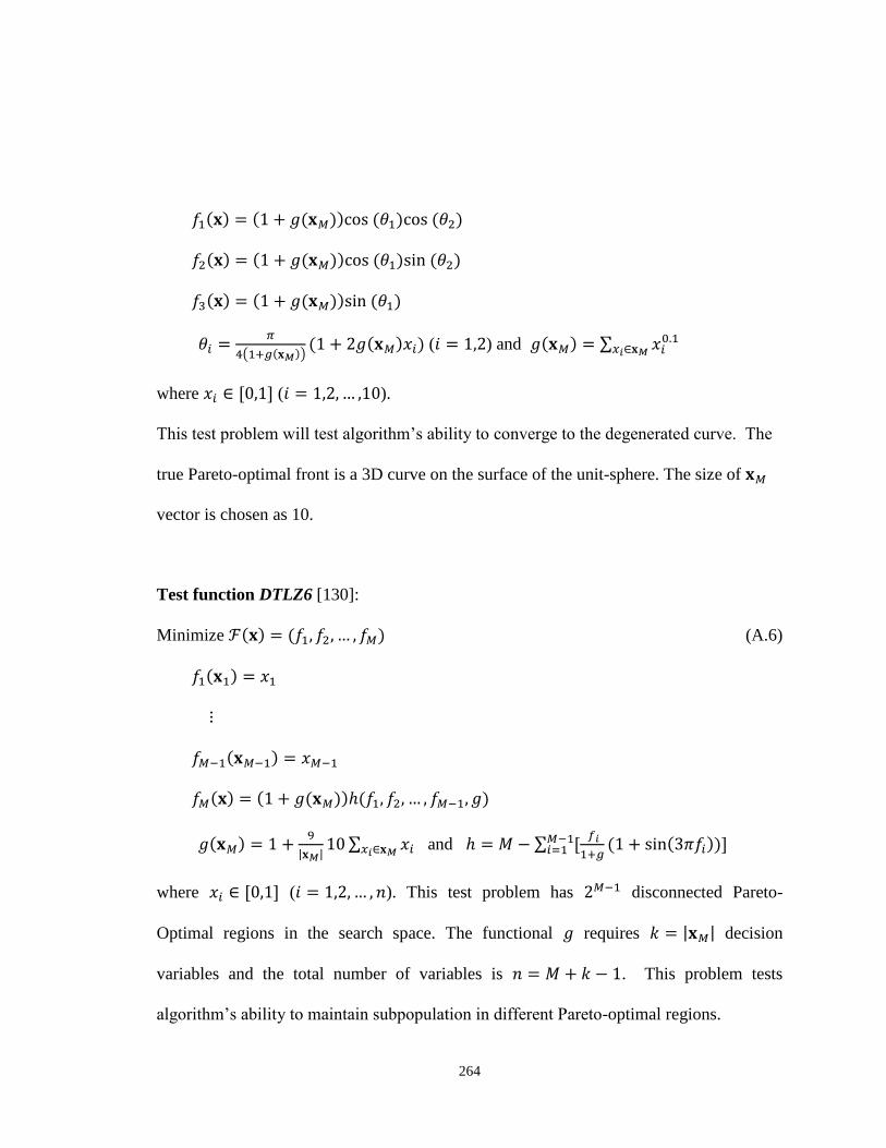
264

( ) and

where ( ).

This test problem will test algorithm’s ability to converge to the degenerated curve. The

true Pareto-optimal front is a 3D curve on the surface of the unit-sphere. The size of

vector is chosen as 10.

Test function DTLZ6 [130]:

Minimize (A.6)

and

where ( ). This test problem has disconnected Pareto-

Optimal regions in the search space. The functional requires decision

variables and the total number of variables is . This problem tests

algorithm’s ability to maintain subpopulation in different Pareto-optimal regions.

265

APPENDIX B

BENCHMARK TEST FUNCTIONS FOR CONSTRAINED OPTIMIZATION

PROBLEMS

All benchmark problems in this Appendix along with the best global minimum found

have been reported from [147].

Test function

Minimize:

(B.1)

Subject to:

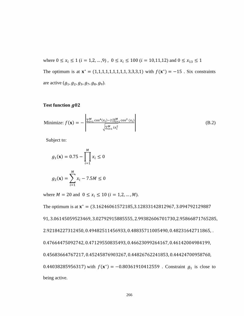
266

where ( ) , ( ) and

The optimum is at with . Six constraints

are active ( ).

Test function

Minimize:

(B.2)

Subject to:

where and ( ).

The optimum is at

.

with . Constraint is close to

being active.

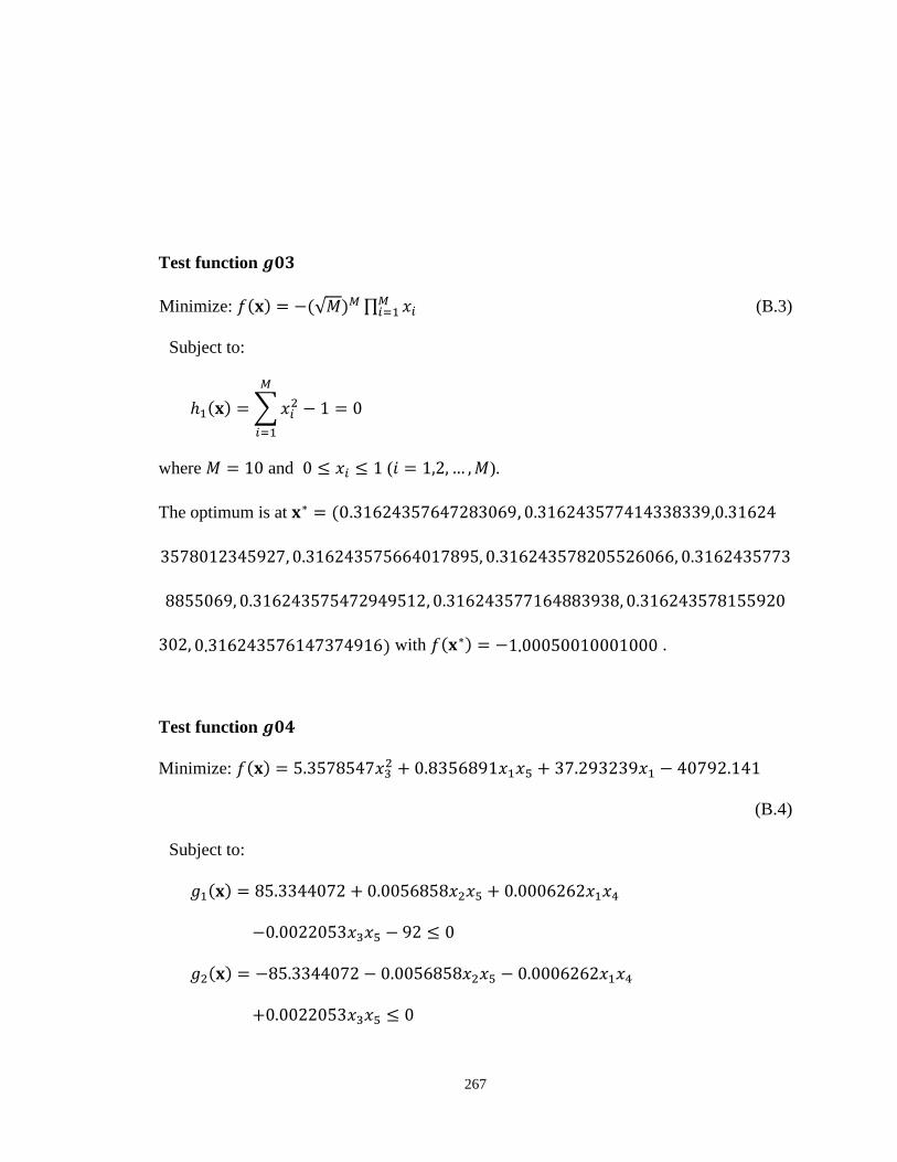
267

Test function

Minimize: (B.3)

Subject to:

where and ( ).

The optimum is at

with .

Test function

Minimize:

(B.4)

Subject to:

268

where , , and ( ).

The optimum is at

, with . Two constraints are active ( ).

Test function

Minimize:

(B.5)

Subject to:

269

where , , and .

The optimum is at

, with .

Test function

Minimize: (B.6)

Subject to:

where , and .

The optimum is at with

. Both constraints are active.

Test function

Minimize:

(B.7)

Subject to:

270

where ( ).

The optimum is at

with

. Six constraints are active ( ).

Test function

Minimize:

(B.8)

Subject to:

where ( ).


.

271

Test function

Minimize:

(B.9)

Subject to:

where ( ).

The optimum is at

with .

Test function

Minimize: (B.10)

Subject to:

272

where , , ( ) and ,

( ).

The optimum is at

with

.

Test function

Minimize: (B.11)

Subject to:

where ( ).


.

Test function

Minimize: (B.12)

Subject to:

273

where ( ) and The feasible region of the search

space consists of 93 disjointed spheres. A point is feasible if and only if there exist

such that the above inequality holds. The optimum is at with .

The solution lies within the feasible region.

Test function

Minimize: (B.13)

Subject to:

where ( ) and ( )

The optimum is at

with .

Test function

Minimize:

(B.14)

Subject to:

274

where ( ) and , , ,

, , , , ,

, .

The optimum is at

with .

Test function

Minimize:

(B.15)

Subject to:

where ( ).

The optimum is at

with .

Test function

Minimize:

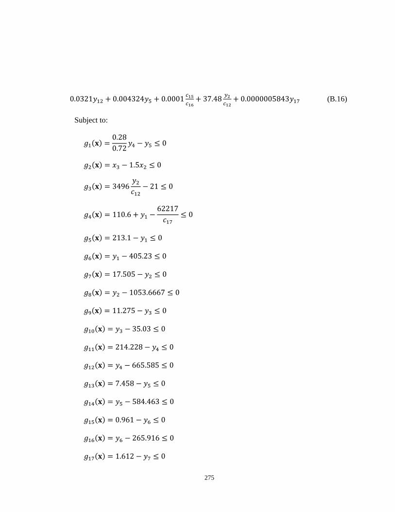
275

(B.16)

Subject to:

276

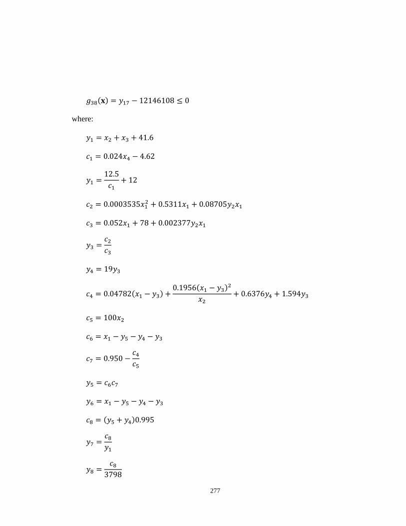
277

where:

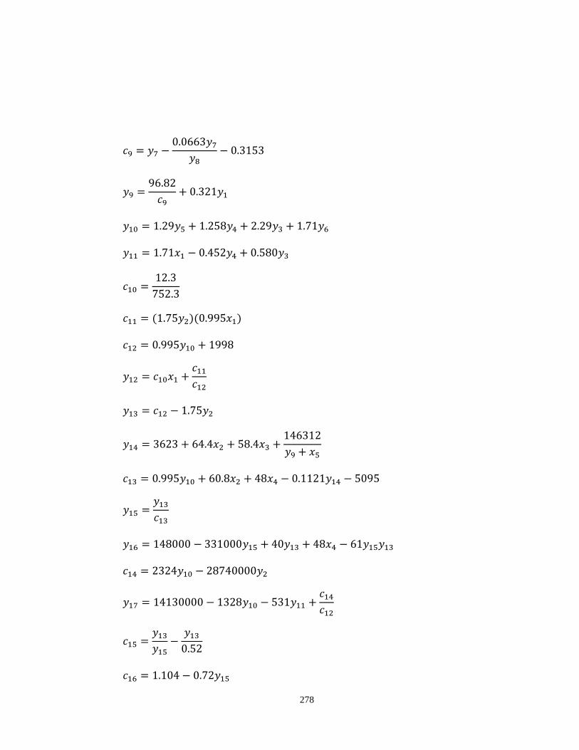
278

279

and where , , ,

, and .

The optimum is at

with

.

Test function

Minimize: (B.17)

where:

Subject to:

280

where , , , ,

, and .

The optimum is at

with

.

Test function

Minimize: (B.18)

Subject to:

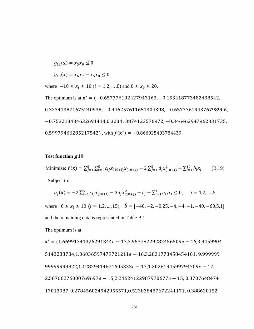
281

where ( ) and .

The optimum is at

, with .

Test function

Minimize:

(B.19)

Subject to:

,

where ( ),

and the remaining data is represented in Table B.1.

The optimum is at

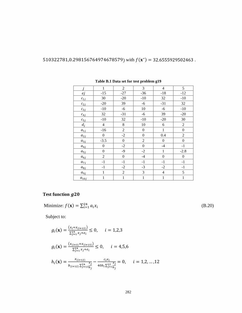
282

with .

Table B.1 Data set for test problem g19

1 2 3 4 5

-15 -27 -36 -18 -12

30 -20 -10 32 -10

-20 39 -6 -31 32

-10 -6 10 -6 -10

32 -31 -6 39 -20

-10 32 -10 -20 30

4 8 10 6 2

-16 2 0 1 0

0 -2 0 0.4 2

-3.5 0 2 0 0

0 -2 0 -4 -1

0 -9 -2 1 -2.8

2 0 -4 0 0

-1 -1 -1 -1 -1

-1 -2 -3 -2 -1

1 2 3 4 5

1 1 1 1 1

Test function

Minimize: (B.20)

Subject to:

,

,

,

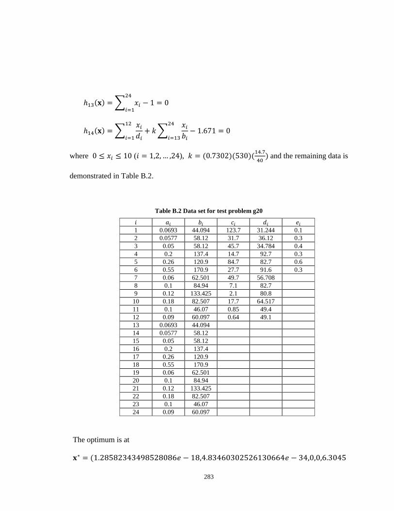
283

where ( ),

and the remaining data is

demonstrated in Table B.2.

Table B.2 Data set for test problem g20

1 0.0693 44.094 123.7 31.244 0.1

2 0.0577 58.12 31.7 36.12 0.3

3 0.05 58.12 45.7 34.784 0.4

4 0.2 137.4 14.7 92.7 0.3

5 0.26 120.9 84.7 82.7 0.6

6 0.55 170.9 27.7 91.6 0.3

7 0.06 62.501 49.7 56.708

8 0.1 84.94 7.1 82.7

9 0.12 133.425 2.1 80.8

10 0.18 82.507 17.7 64.517

11 0.1 46.07 0.85 49.4

12 0.09 60.097 0.64 49.1

13 0.0693 44.094

14 0.0577 58.12

15 0.05 58.12

16 0.2 137.4

17 0.26 120.9

18 0.55 170.9

19 0.06 62.501

20 0.1 84.94

21 0.12 133.425

22 0.18 82.507

23 0.1 46.07

24 0.09 60.097

The optimum is at

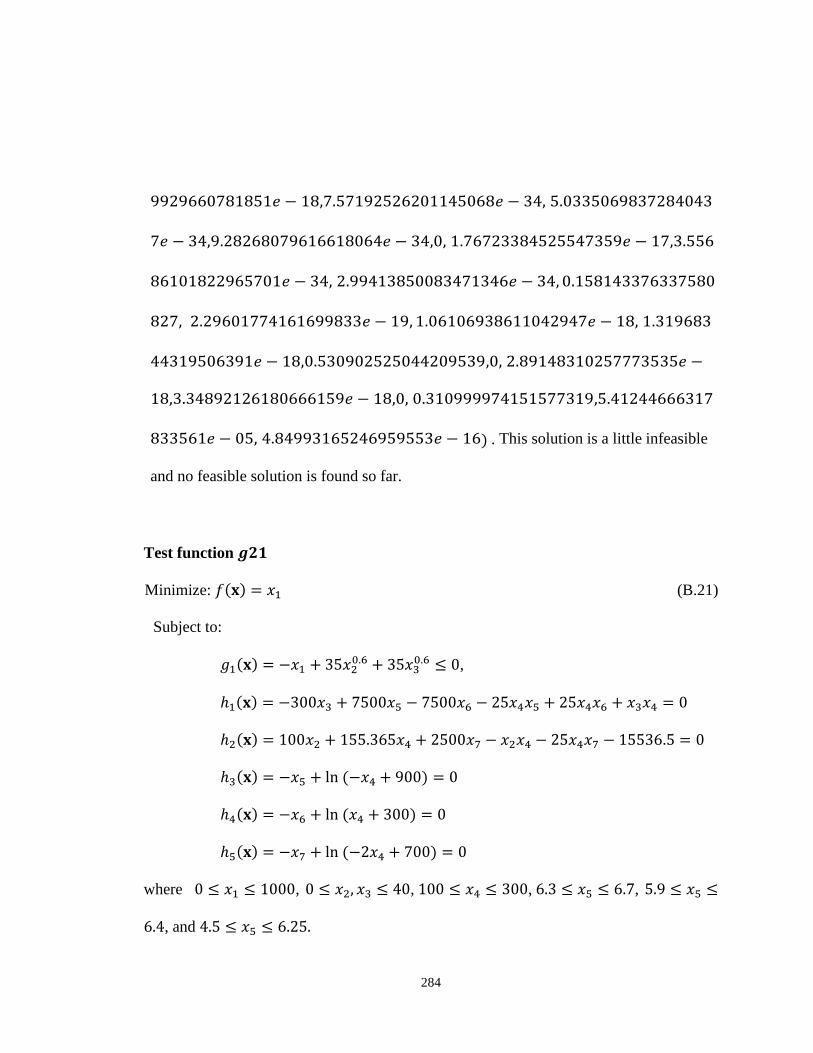
284

. This solution is a little infeasible

and no feasible solution is found so far.

Test function

Minimize: (B.21)

Subject to:

,

where , , , ,

, and

285

The optimum is at

with .

Test function

Minimize: (B.22)

Subject to:

,

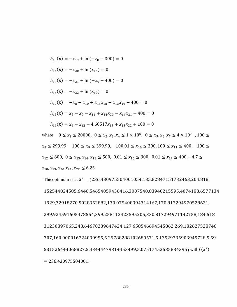
286

where , , ,

, , ,

The optimum is at

with

.

287

Test function

Minimize: (B.23)

Subject to:

,

where , , , and

.

The optimum is at

with .

Test function

Minimize: (B.24)

Subject to:

288

,

where , and . The feasible region consist two disconnected sub-

regions.


289

APPENDIX C

BENCHMARK TEST FUNCTIONS FOR DYNAMIC OPTIMIZATION

PROBLEMS

Test functions MP1 [166]:

Moving Cone Peaks Benchmark Problem is a maximization problem which has

components as moving competing cones with independently varying height, width and

location formulated as:

)))(),(),(,(max),(max(),(,...,2,1

1Mi

iiiMP ttwthPBtf

pxxx (C.1)

where )(xB is a time-invariant basis landscape and P is a function that defines cone-

shaped peaks with M peaks whose height ( ih ), width ( iw ), and location ( ip ) are time-

varying.

Test functions DF2 [167]:

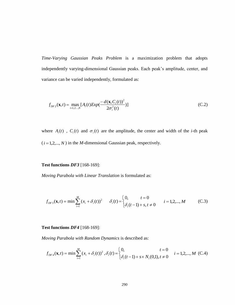
290

Time-Varying Gaussian Peaks Problem is a maximization problem that adopts

independently varying-dimensional Gaussian peaks. Each peak’s amplitude, center, and

variance can be varied independently, formulated as:

)])(2

))(,(()([max),(

2

2

...,2,12

t

tCdExptAtf

i

ii

NiDF

xx

(C.2)

where )(tAi , )(tCi and )(ti are the amplitude, the center and width of the i-th peak

( Ni ,...,2,1 ) in the M-dimensional Gaussian peak, respectively.

Test functions DF3 [168-169]:

Moving Parabola with Linear Translation is formulated as:

M

i

iiDF txtf1

2

3 ))((min),( x

0 ,)1(

0 ,0)(

tst

tt

i

i

Mi ,...,2,1 (C.3)


Moving Parabola with Random Dynamics is described as:

M

i

iiDF txtf1

2

4 ))((min),( x ,

0 ),1,0()1(

0 ,0)(

tNst

tt

ii

i

Mi ,...,2,1 (C.4)

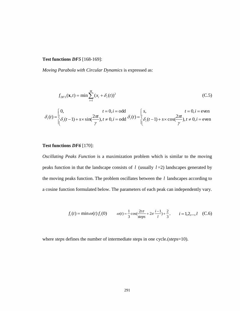
291


Moving Parabola with Circular Dynamics is expressed as:

M

i

iiDF txtf1

2

5 ))((min),( x (C.5)

odd,0 ),

2sin()1(

odd,0 ,0

)(it

tst

it

ti

i

even,0 ),

2cos()1(

even,0 ,

)(it

tst

its

ti

i

Test functions DF6 [170]:

Oscillating Peaks Function is a maximization problem which is similar to the moving

peaks function in that the landscape consists of l (usually l =2) landscapes generated by

the moving peaks function. The problem oscillates between the l landscapes according to

a cosine function formulated below. The parameters of each peak can independently vary.

)0()(min)( ii fttf ,3

2)

12

2cos(

3

1)(

l

i

steps

tt

li ,...,2,1 (C.6)

where steps defines the number of intermediate steps in one cycle.(steps=10).

VITA

Moayed Daneshyari

Candidate for the Degree of

Doctor of Philosophy

Thesis: CULTURAL PARTICLE SWARM OPTIMIZATION

Major Field: Electrical and Computer Engineering

Biographical:

Education: Received B.S. in Electrical Engineering from Sharif University of

Technology in 1995, M.S. in Biomedical Engineering from Iran University of

Science and Technology in 1998, M.S. in Physics from Oklahoma State

University in 2007, Ph.D. in Electrical and Computer Engineering from

Oklahoma State University in 2010.

Experience: Employed at IranKhodro Automobile Manufacturer as Control

Engineer (1994), Nozohour Pulp and Paper Co. as Automation Engineer

(1995-96), Chamran Hospital as Biomedical Engineer (1996), School of

Cognitive Science in Institute for Research in Fundamental Science as

Research Fellow (1996-97), Namdar Electrical Eng. Inc. as Engineer (1997-

99), FanAvaran RizAfzar Co. as Design Engineer (1999-00), Namvaran Oil

Consultant Inc. as Instrumentation Engineer (2000), Oklahoma State

University, Dept. of Physics as Teaching Assistant (2001-07), Oklahoma State

University, Dept. of Electrical and Computer Eng. As Teaching Assistant and

Research Assistant (2004-2008), and Elizabeth City State University as

Assistant Professor (2008-present)

Professional Memberships: The Institute of Electrical and Electronics Engineers

(IEEE) since 1996; IEEE Computational Intelligence Society since 2006,

IEEE Engineering in Medicine and Biology Society since 1996,IEEE

Systems, Man, and Cybernetics Society since 1996, Association of

Technology, Management, and Applied Engineering (ATMAE) since 2009.

CULTURAL PARTICLE SWARM OPTIMIZATION - CORE

Documents