Cubic Functions, their Roots and the Family of Secant Lines that Relate Them

Cubic Functions, their Roots

and the Family of Secant Lines that

Relate Them

by

John W. Losse and Frank J. [email protected]

[email protected]

Scottsdale Community College

Department of Mathematics

Scottsdale, AZ 85256

1

ABSTRACT: A well-known property of cubic functions is this:

the tangent line to the graph of a cubic at the average of

any two of its real zeros also passes through the graph at

the third zero. In this paper, we show how the result

extends to all members of a certain family of “symmetric

secant lines of the function”—even when two of the zeros of

the cubic are complex. We also identify a “graphical

signature” of the complex zeros of f, i.e., we show how the

real and imaginary parts of a complex zero of a cubic

function f are related to certain features of its graph.

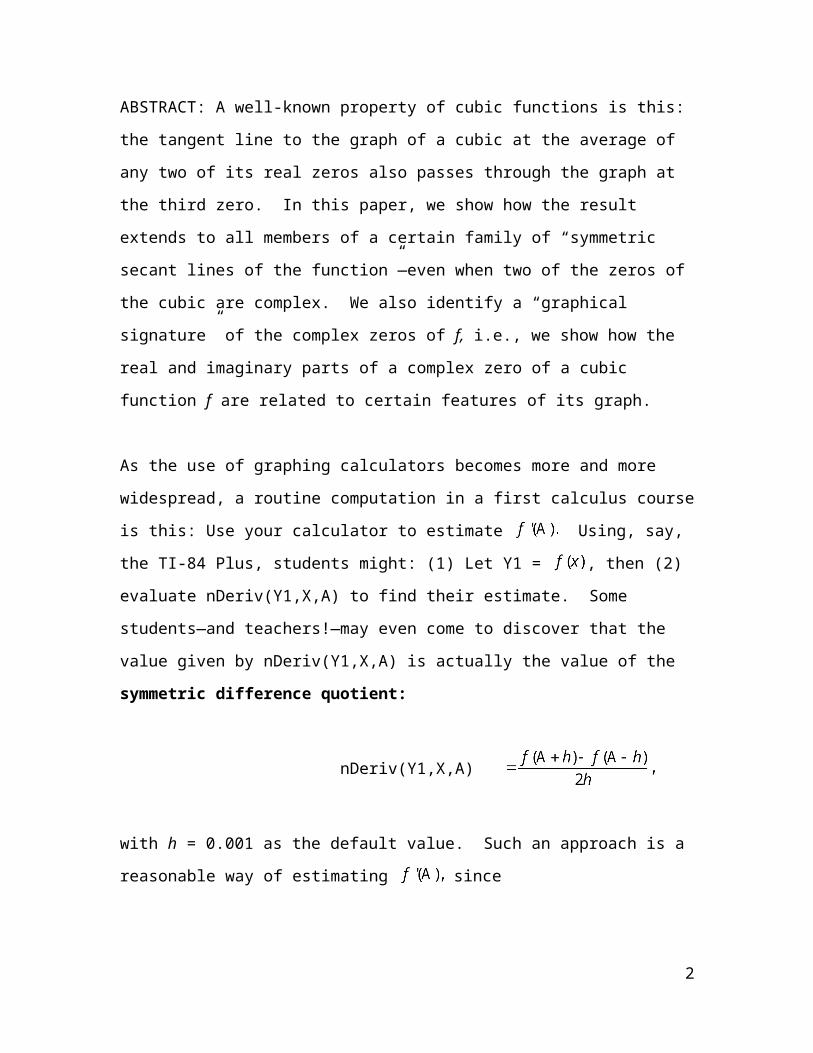
As the use of graphing calculators becomes more and more

widespread, a routine computation in a first calculus course

is this: Use your calculator to estimate Using, say,

the TI-84 Plus, students might: (1) Let Y1 = , then (2)

evaluate nDeriv(Y1,X,A) to find their estimate. Some

students—and teachers!—may even come to discover that the

value given by nDeriv(Y1,X,A) is actually the value of the

symmetric difference quotient:

nDeriv(Y1,X,A)

with h = 0.001 as the default value. Such an approach is a

reasonable way of estimating since

2

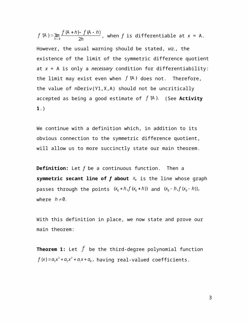
, when f is differentiable at x = A.

However, the usual warning should be stated, viz., the

existence of the limit of the symmetric difference quotient

at x = A is only a necessary condition for differentiability:

the limit may exist even when does not. Therefore,

the value of nDeriv(Y1,X,A) should not be uncritically

accepted as being a good estimate of (See Activity

1.)

We continue with a definition which, in addition to its

obvious connection to the symmetric difference quotient,

will allow us to more succinctly state our main theorem.

Definition: Let f be a continuous function.  Then a

symmetric secant line of f about is the line whose graph

passes through the points and

where

With this definition in place, we now state and prove our

main theorem:

Theorem 1: Let be the third-degree polynomial function

having real-valued coefficients.

3

(i) If p is the average of two of the real zeros of f, then

every symmetric secant line of f about p passes through

the third zero of f.

(ii) If p is the average of the complex zeros of f, then

every symmetric secant line of f about p passes through

the third zero of f.

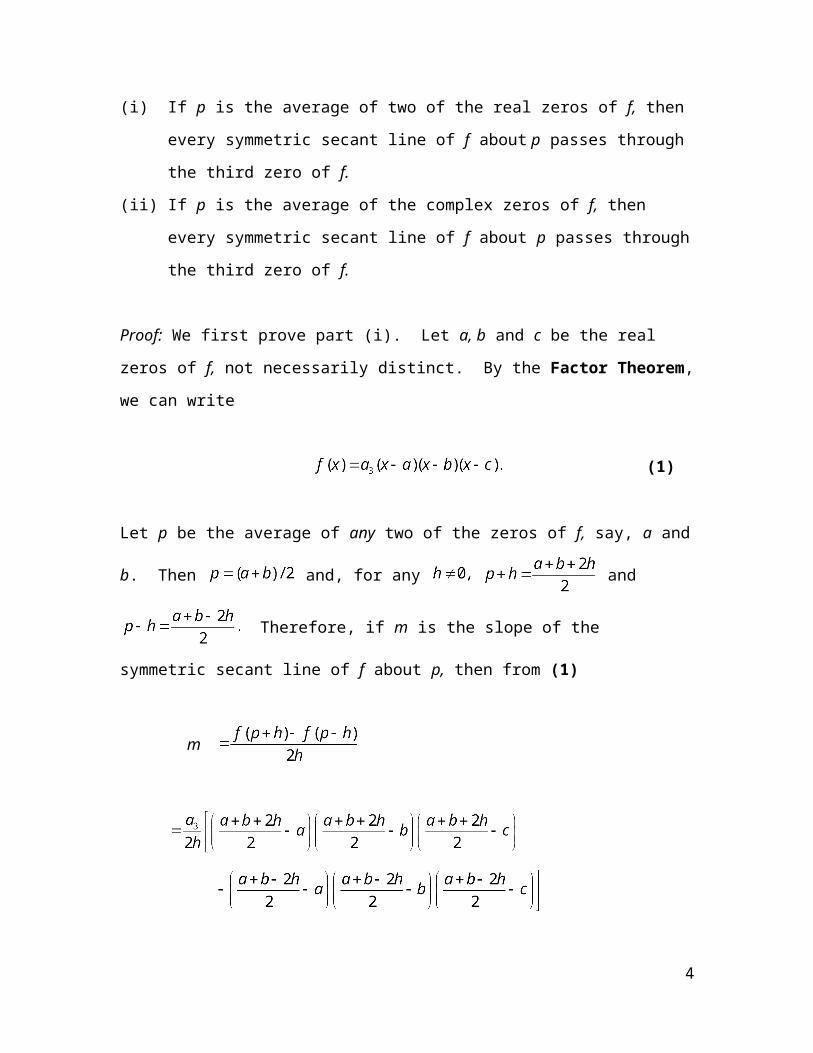
Proof: We first prove part (i). Let a, b and c be the real

zeros of f, not necessarily distinct. By the Factor Theorem,

we can write

(1)

Let p be the average of any two of the zeros of f, say, a and

b. Then and, for any and

Therefore, if m is the slope of the

symmetric secant line of f about p, then from (1)

m

4

,

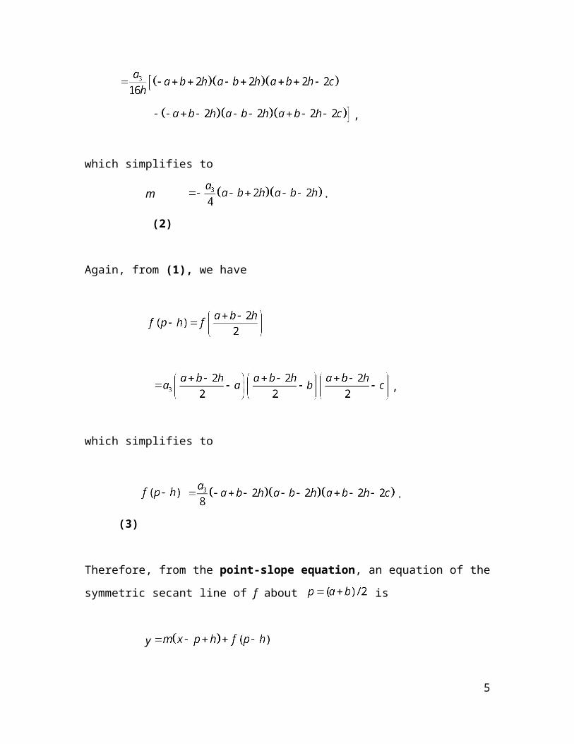
which simplifies to

m .

(2)

Again, from (1), we have

,

which simplifies to

.

(3)

Therefore, from the point-slope equation, an equation of the

symmetric secant line of f about is

y

5

(4)

Substituting (2) and (3) into (4), gives

y

.

Simplifying, we have

y

or

y .

(5)

From (5), we see that, independent of the value of h, the graph of

the symmetric secant of f about has its x-

intercept at the point (c, 0) –i.e., at the point given by

the third (real) zero of f. This completes the proof of

part (i).

6

To prove part (ii), recall that, since f has real-valued

coefficients, the complex zeros of f occur in conjugate

pairs. Let r and be the zeros of f. Again, by the

Factor Theorem, we can write

. (6)

Let p be the average of the complex zeros of f. Then

and, for any and

Therefore, if M is the slope of the symmetric secant line

of f about p, then from (6)

M

,

or, finally,

7

M .

(7)

Again, from (6), we have

i.e.,

(8)

Therefore, a point-slope equation of the symmetric secant

line of f about is

y

(9)

From (7) and (8), (9) becomes

y ,

which simplifies to

8

y ,

or

y

(10)

From (10), we see that, independent of the value of h, the graph of

the symmetric secant of f about has its

x-intercept at the point (r, 0) –i.e., at the point given by

the real zero of f. This completes the proof of part (ii)

and, hence, our proof of Theorem 1.

Moving from secant to tangent lines

Before graphically illustrating our results, consider what

happens when h approachs 0. We first do this for the case

when the zeros of f are real-valued. In (1), where

, we found that, for any the slope

m of a symmetric secant line of f about is given

by

m

(2)

9

and, hence,

(11)

On the other hand, since

,

then

(12)

10

From (11) and (12), we see that , i.e., the slope

of a symmetric secant line of f about converges

to that of the tangent line at p. This is as expected,

since f is differentiable and is the

symmetric difference quotient of f about It also

means that the family of symmetric secant lines of f about p

converge to the tangent line to the graph of at p; in fact, the

equation for a symmetric secant line of f about :

y

(5)

becomes, at h = 0, the equation of the tangent line of f at

p:

y

(13)

From (13), we see that the tangent line to the graph of

at also passes through the

x-intercept of determined by the third zero: (c, 0)—

a fact that, as stated in the abstract of this paper, is

already well-known. Figure 1 below illustrates the

results, using

11

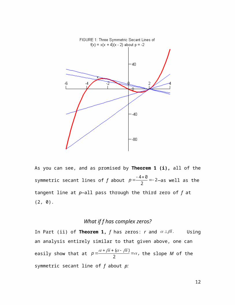
As you can see, and as promised by Theorem 1 (i), all of the

symmetric secant lines of f about —as well as the

tangent line at p—all pass through the third zero of f at

(2, 0).

What if f has complex zeros?

In Part (ii) of Theorem 1, f has zeros: r and Using

an analysis entirely similar to that given above, one can

easily show that at the slope M of the

symmetric secant line of f about p:

12

M

(7)

converges to as Furthermore, the

family of symmetric secant lines of f about whose

equations are:

y

(10)

converge to:

y

(14)

From (14), we see that the tangent line to the graph of

at

also passes through the x-intercept at (r,

0). In Figure 2 below we illustrate the result, using:

which has zeros: -2 and and, hence,

13

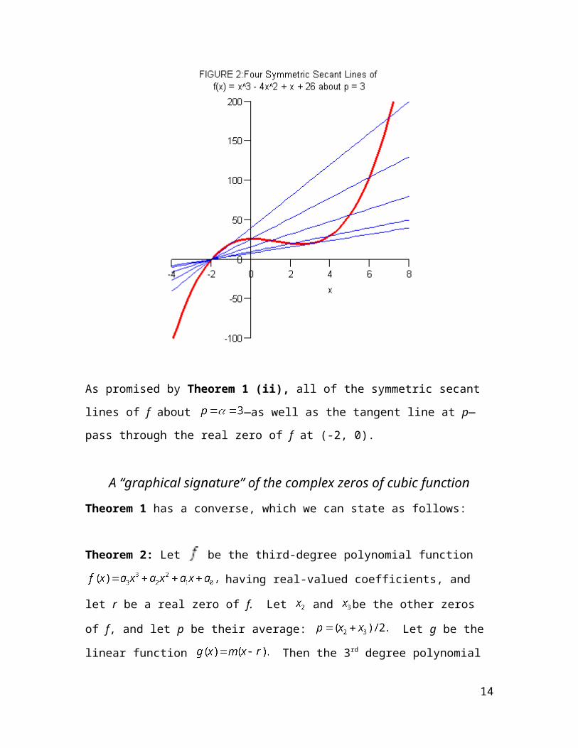
As promised by Theorem 1 (ii), all of the symmetric secant

lines of f about —as well as the tangent line at p—

pass through the real zero of f at (-2, 0).

A “graphical signature” of the complex zeros of cubic function

Theorem 1 has a converse, which we can state as follows:

Theorem 2: Let be the third-degree polynomial function

having real-valued coefficients, and

let r be a real zero of f. Let and be the other zeros

of f, and let p be their average: Let g be the

linear function Then the 3rd degree polynomial

14

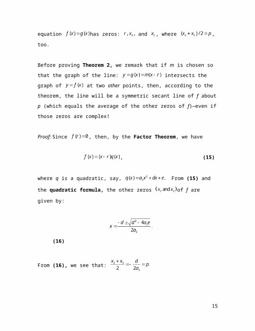
equation has zeros: and , where ,

too.

Before proving Theorem 2, we remark that if m is chosen so

that the graph of the line: intersects the

graph of at two other points, then, according to the

theorem, the line will be a symmetric secant line of f about

p (which equals the average of the other zeros of f)—even if

those zeros are complex!

Proof: Since , then, by the Factor Theorem, we have

, (15)

where q is a quadratic, say, From (15) and

the quadratic formula, the other zeros of f are

given by:

x

(16)

From (16), we see that:

15

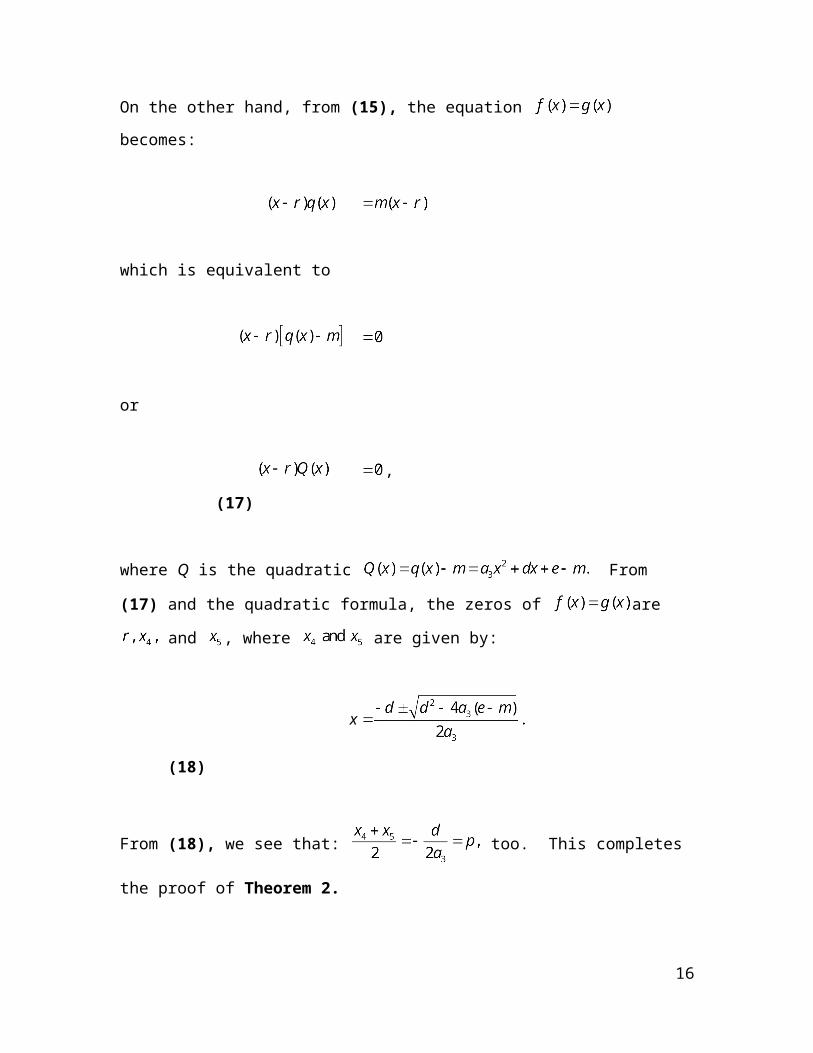
On the other hand, from (15), the equation

becomes:

which is equivalent to

or

,

(17)

where Q is the quadratic From

(17) and the quadratic formula, the zeros of are

and , where are given by:

x

(18)

From (18), we see that: too. This completes

the proof of Theorem 2.

16

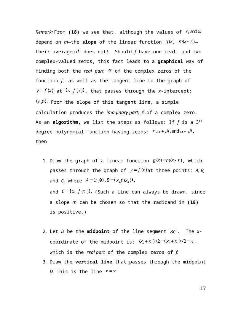
Remark: From (18) we see that, although the values of

depend on m—the slope of the linear function —

their average does not! Should f have one real- and two

complex-valued zeros, this fact leads to a graphical way of

finding both the real part, of the complex zeros of the

function f, as well as the tangent line to the graph of

at , that passes through the x-intercept:

From the slope of this tangent line, a simple

calculation produces the imaginary part, of a complex zero.

As an algorithm, we list the steps as follows: If f is a 3rd

degree polynomial function having zeros:

then

1. Draw the graph of a linear function , which

passes through the graph of at three points: A, B,

and C, where

and (Such a line can always be drawn, since

a slope m can be chosen so that the radicand in (18)

is positive.)

2. Let D be the midpoint of the line segment . The x-

coordinate of the midpoint is: —

which is the real part of the complex zeros of f.

3. Draw the vertical line that passes through the midpoint

D. This is the line

17

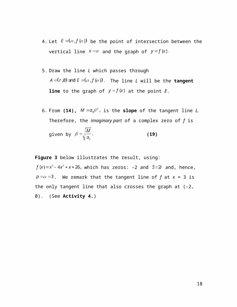
4. Let be the point of intersection between the

vertical line and the graph of

5. Draw the line L which passes through

The line L will be the tangent

line to the graph of at the point E.

6. From (14), is the slope of the tangent line L.

Therefore, the imaginary part of a complex zero of f is

given by (19)

Figure 3 below illustrates the result, using:

which has zeros: -2 and and, hence,

. We remark that the tangent line of f at x = 3 is

the only tangent line that also crosses the graph at (-2,

0). (See Activity 4.)

18

With and L tangent to f at the point

, its slope is Since from

(19) we have Therefore, as expected, the

complex zeros of f are: and

Classroom Activities:

1. Use nDeriv to estimate the derivative of and

at x = 0. Should the values found be accepted

as accurate estimates? Explain.

2. Let f be the quadratic function defined by .

19

a. Find the slopes of the symmetric secant lines of f

about p = 4, for the following values of h: 3, 2, 1,

0.1, 0.01. How do their values compare?

b. Compute the value of the derivative at p = 4.

c. Prove the following Theorem: Let be a quadratic

function having real-valued coefficients. Then, at any

, the slope m of every symmetric secant line of f

about equals the value of the derivative of f at ,

i.e., .

3. Let be the quadratic function with

real-valued coefficients. Suppose are the complex

zeros of f. Follow the following steps in order to find a

“graphical signature” for the real and imaginary parts

of the zeros of f.

a. Use the Factor Theorem to find a formula for

b. By completing the square, rewrite the formula from part

a in vertex form and identify the coordinates of its

vertex. (Labeling a “typical graph” of f may help.)

c. Evaluate f at (not ). How do these

value(s) of f(x) compare with its value at the vertex?

Indicate this on your “typical graph.”

d. Finally, identify the graphical signature of the real

and imaginary parts of the complex zeros of f.

20

4. Let f be the cubic function defined by ,

with real-valued coefficients. Prove that any tangent

line to the graph of crosses the graph at only one

point and that no two tangent lines cross the graph at

the same point. Hint: Choose some Rewrite the

formula for using its 3rd-degree Taylor polynomial

at

21