CT – 3: Equilibrium calculations: Minimizing of Gibbs energy, equilibrium conditions as a set of equations, global minimization of Gibbs energy, driving.

CT – 3: Equilibrium calculations:

Minimizing of Gibbs energy, equilibrium conditions as a set of equations, global minimization of Gibbs energy, driving force for a phase

Equilibrium conditions

dU = T.dS-p.dV + j j.dnj (see CT-2)Conjugated properties: T,p,j – intensive, S,V,nj – extensive

At constant entropy, volume, and nj , equilibrium is characterized by minimum of the internal energy.

Most proper conditions: p,T,nj

dG = V dp – S dT + j j dnj

(mole fraction: xi = ni/N, N = j nj)

G may have several minima. That with the most negative value of G is „global minimum“ which

corresponds to the „stable equlibrium“ and another ones are „local minima“ and correspond to the „metastable equilibria“

Stable and metastable states

Metastable state

Stable state

Unstable stateUnstable state

Metastable state

Stable state

Equilibrium conditions – cont.

For determination of phases presented in equilibrium: analytical expression of G needed.

Total Gibbs energy:

G = m.Gm (m 0, it is amount of phase )

Amount of components i: Ni = N.xio

Introduce: xi = m. x i - lever rule

Equilibrium condition:

min (G) = min ( m. Gm(T,P, x

i or y (l,)k ))

(xi is definite function of yk

(l, ); m, x i are unknowns)

6

• Rule 1: If we know T and Co, then we know: --the composition and types of phases present.

• Example:

wt% Ni20 40 60 80 10001000

1100

1200

1300

1400

1500

1600T(°C)

L (liquid)

(FCC solid solution)

L +

liquidus

solid

us

A(1100,60)B

(1250,3

5)

Cu-Niphase

diagramA(1100, 60): 1 phase:

B(1250, 35): 2 phases: L +

Adapted from Fig. 9.2(a), Callister 6e.(Fig. 9.2(a) is adapted from Phase Diagrams of Binary Nickel Alloys, P. Nash (Ed.), ASM International, Materials Park, OH, 1991).

PHASE DIAGRAMS: composition and types of phases

7

• Rule 2: If we know T and Co, then we know: --the composition and amount of each phase.

• Example:

wt% Ni20

1200

1300

T(°C)

L (liquid)

(solid)L +

liquidus

solidus

30 40 50

TAA

DTD

TBB

tie line

L +

433532CoCL C

Cu-Ni system

At TA: Only Liquid (L) CL = Co ( = 35wt% Ni)

At TB: Both and L CL = Cliquidus ( = 32wt% Ni here) C = Csolidus ( = 43wt% Ni here)

At TD: Only Solid () C = Co ( = 35wt% Ni)

Co = 35wt%Ni

Adapted from Fig. 9.2(b), Callister 6e.(Fig. 9.2(b) is adapted from Phase Diagrams of Binary Nickel Alloys, P. Nash (Ed.), ASM International, Materials Park, OH, 1991.)

PHASE DIAGRAMS: composition and amount of phases

Lever rule: mL/m = CoC/CoCL

Types of phase diagrams of Cu

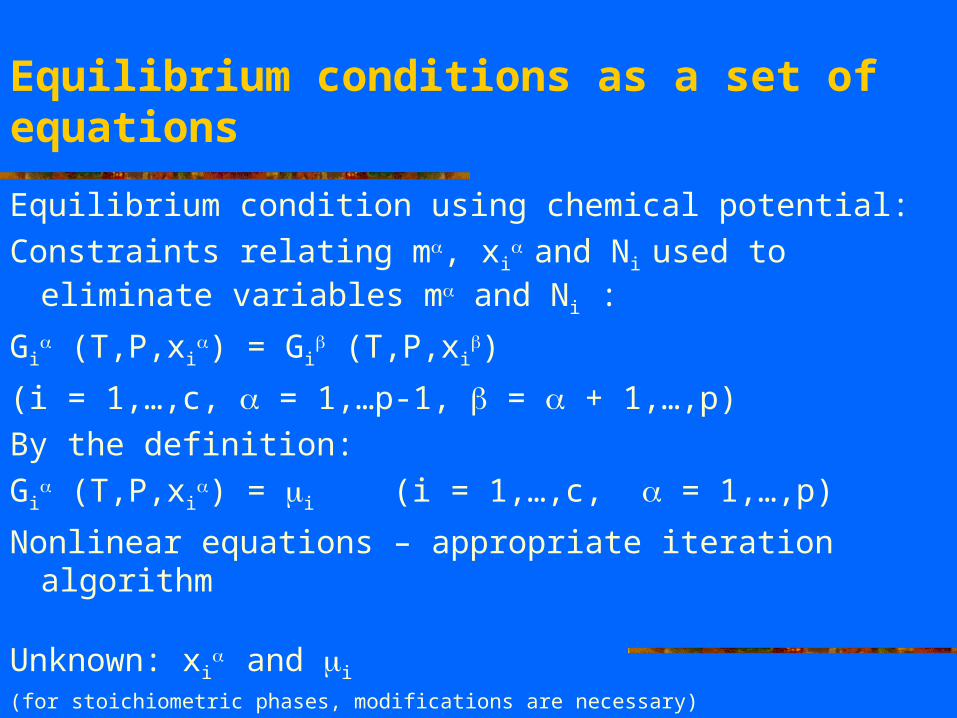
Equilibrium conditions as a set of equations

Equilibrium condition using chemical potential:

Constraints relating m, xi and Ni used to eliminate

variables m and Ni :

Gi (T,P,xi

) = Gi (T,P,xi

)

(i = 1,…,c, = 1,…p-1, = + 1,…,p)

By the definition:

Gi (T,P,xi

) = i (i = 1,…,c, = 1,…,p)

Nonlinear equations – appropriate iteration algorithm

Unknown: xi and i

(for stoichiometric phases, modifications are necessary)

Gm as function of site fractions yk

(l, )

instead of mole fractions xi

Lagrange-multiplier method

Constraints:

(1) Total amount of each component Ni is kept constant

(2) Sum of site fractions in each sublattice is equal 1

(3) Sum of charge of ionic species in each phase is equal 0

Constraints mathematically

LFS - CT

Lagrange-multiplier method-cont.

Each constraint is multiplied by „Lagrange multiplier“ and added to the total Gibbs energy

min (G) = min ( m. Gm(T,P, x

i or y (l,)k ))

to get a sum L.

If all constraints are satisfied, L is equal to G and a minimum of L is equivalent to a minimum of the total Gibbs energy G.

Newton‘s method

To find x for which y=0: (also for searching the minimum of Gm) (df/dx)x=xi . xi = -f(xi), xi+1 = xi + xi There exists cases, where this method diverges

LFS - CT

There exists cases, where Newton‘s method diverges

Starting with x1 - divergesStarting with x3 – solution on the left,

Starting with x4 – solution on the right,

x5, x6 - finally on the left – influence of starting values on the result of minimization

LFS - CT

Newton-Raphson method

It is extension of Newton‘s method to more than one variable (n equations for n unknowns).

All iterative techniques like the Newton-Raphson one need an initial constitution for each phase in order to find the minimum of Gibbs energy surface for the given conditions.

Thermocalc – starting point tools

Automatic starting values

Set-all-start values

Global minimization of the Gibbs energyMiscibility gap problem (solution phases only)

LFS - CT

Compounds with fixed compositions

Equilibrium set of phases is given by the tangent „hyperplane“ defined by the Gibbs energies of a set of compounds constrained by the given overall composition and with no compound with a Gibbs energy below this hyperplane („global“ minimum).

Gibbs energies of a set of compounds

A xB B

G/kJ.mol-1

LFS -CT

Minimization techniques to find global equilibrium

Gibbs energy surface of all solution phases is approximated with a large number of „compounds“ which Gibbs energy has the same value as the solution phase at the composition of the compound (dense grid about 104 (100x100) compounds, for multicomponent system about 106 such compounds)

Search for hyperplane representing equlibrium for the compounds is then carried out.

Minimization techniques to find global equilibrium

When minimum for these „compounds“ has been found, the „compound“ in this equilibrium set must be identified with regard to which solution phase they belong to.

Each „compound“ --- initial constitution of the solution phase --- is used in a Newton-Raphson calculation to find the equilibrium for the solution phases (correct, not wrong)

Limitation of the method to find the global equilibrium

T, p and overall composition must be known

For other conditions as starting point (e.g. activity of components) –-- indirect procedure:

Overall composition calculate first and use it for a new equilibrium calculation.

Conditions for a single equilibrium

The equilibrium conditions as a set of equations contain fewer equation than unknowns – the difference = number of degrees of freedom „f“

Therefore: „f“ extra conditions (equations) must be added to select definitely single equilibrium

„Unknown state variable“ = „constant value“ :

Example:

For binary system i-j: (f=0)

T = 1273, p = 101352, xi = 0.1, i = -40000

Thermocalc: Fe – W – Cr system

set-condition t=1273 x(W)=0.15 x(Cr)=0.35 p=1E5 n=1

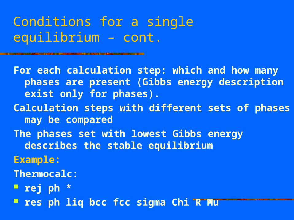
Conditions for a single equilibrium – cont.

For each calculation step: which and how many phases are present (Gibbs energy description exist only for phases).

Calculation steps with different sets of phases may be compared

The phases set with lowest Gibbs energy describes the stable equilibrium

Example:

Thermocalc: rej ph * res ph liq bcc fcc sigma Chi R Mu

Example

Different starting points may give different sets of equilibrium phases for the same overall composition.

Check the total Gibbs energy for global minimum

(In new codes checked automatically.)

Ag-In system

Output from POLY-3, equilibrium number = 1, Ag-In systemConditions: T=500, X(IN)=2E-1, P=100000, N=1 DEGREES OF FREEDOM 0

Temperature 500.00, Pressure 1.000000E+05 Number of moles of components 1.00000E+00, Mass 1.09260E+02 Total Gibbs energy -3.15128E+04, Enthalpy -1.91077E+02, Volume 0.00000E+00

Overal compositionComponent Moles W-Fraction Activity Potential Ref.state AG 8.0000E-01 7.8982E-01 1.6046E-03 -2.6752E+04 SER

IN 2.0000E-01 2.1018E-01 5.2290E-06 -5.0558E+04 SER FCC_A1#1 Status ENTERED Driving force 0.0000E+00 Number of moles 5.6253E-01, Mass 6.1400E+01 Mass fractions: AG 8.06153E-01 IN 1.93847E-01

HCP_A3#1 Status ENTERED Driving force 0.0000E+00 Number of moles 4.3747E-01, Mass 4.7860E+01 Mass fractions: AG 7.68872E-01 IN 2.31128E-01

Mapping a phase diagram

2 or 3 variables of the conditions are selected as axis variables with lower and upper limit and maximal step.

All additional conditions – kept constant throughout the whole diagram

Start: „initial equilibrium“ for Newton-Raphson calculation (with all phases „entered“)

All results of calculations usually stored – any phase diagram may be displayed at the end of calculations

Mapping a phase diagram – cont.

Example (in Thermocalc):

set-axis-variable 1 x(Ag) 0 1 .025

s-a-v 2 t 300 1200 10

map

(T in K)

„Stepping“

By stepping with small decrements of the temperature (or enthalpy or amount liquid phase-generally one variable) one can determine the new composition of the liquid and then remove the amount of solid phase formed by resetting the overall composition to the new liquid composition before taking the next step

(Scheil solidification scheme: no diffusion in solid phase, high diffusion in liquid phase)

Example – Scheil-Gulliver solidification scheme

xNi = 0.1

Azeotropic points

Maxima and minima of binary two-phase fields

Setting additional conditions

For binary: x - x = 0

For ternary: xB - xB

= 0

xC - xC

= 0

The driving force for a phase

LFS - CT

Driving force-application

Driving force ΔG, GFCC: (Fig.2.5)(difference in G of paralel tangents for phases and

stability tangent)

- theory of nucleation of phases- minimization of G (whether another phases set

exists that is more stable than calculated set of phases)

Conditions for a single equilibrium – cont.

Adding phase to the calculated stable phase set:

Positive „driving force“ of the phase – repeat calculation

Removing phase from the selected set:

Calculation finds negative amount for one of selected phases

Conditions for a single equilibrium – cont.

Phases with miscibility gaps may have more than one driving force at different compositions – test must be performed for each of these compositions

Test by experiment when some phases appear in calculations to be stable but experimentally are found to be not stable

Questions for learning

1.What is a difference between stable and metastable states?

2. What is principle of Lagrange-multiplier method?

3. What is principle of Newton – Raphson method?

4. What conditions must be fulfilled for single equilibrium calculation?

5. What means „mapping“ and „stepping“ in calculations of phase equilibria?