CSE 373: Analysis of Algorithms Lectures 5 ‒ 8 ( Correctness of Algorithms ) Rezaul A. Chowdhury Department of Computer Science SUNY Stony Brook Fall 2014

Welcome message from author
This document is posted to help you gain knowledge. Please leave a comment to let me know what you think about it! Share it to your friends and learn new things together.
Transcript
CSE 373: Analysis of Algorithms
Lectures 5 ‒ 8
( Correctness of Algorithms )
Rezaul A. Chowdhury
Department of Computer Science
SUNY Stony Brook
Fall 2014
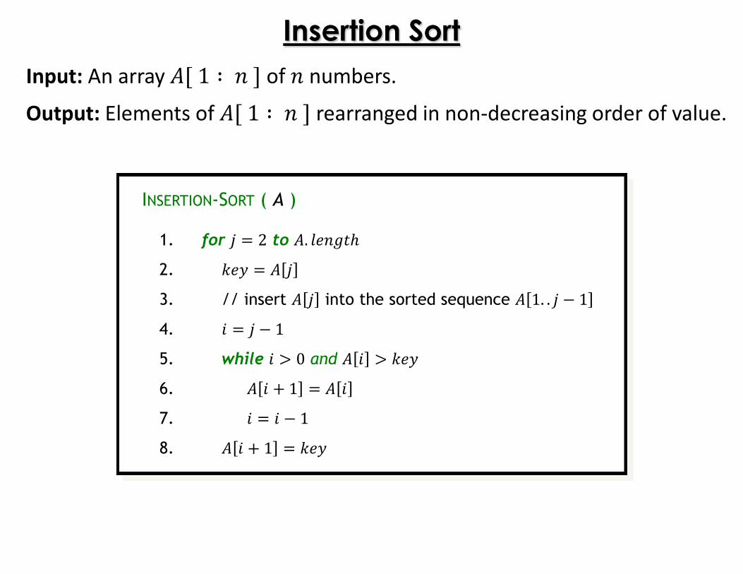
Insertion Sort
Input: An array ��1 ∶ �� of � numbers.
Output: Elements of ��1 ∶ �� rearranged in non-decreasing order of value.
INSERTION-SORT ( A )
1. for � 2 to �. � ����2. � � � �3. // insert � � into the sorted sequence � 1. . � � 14. � � � 15. while � � 0 and � � � � �6. � � � 1 � �7. � � � 18. � � � 1 � �
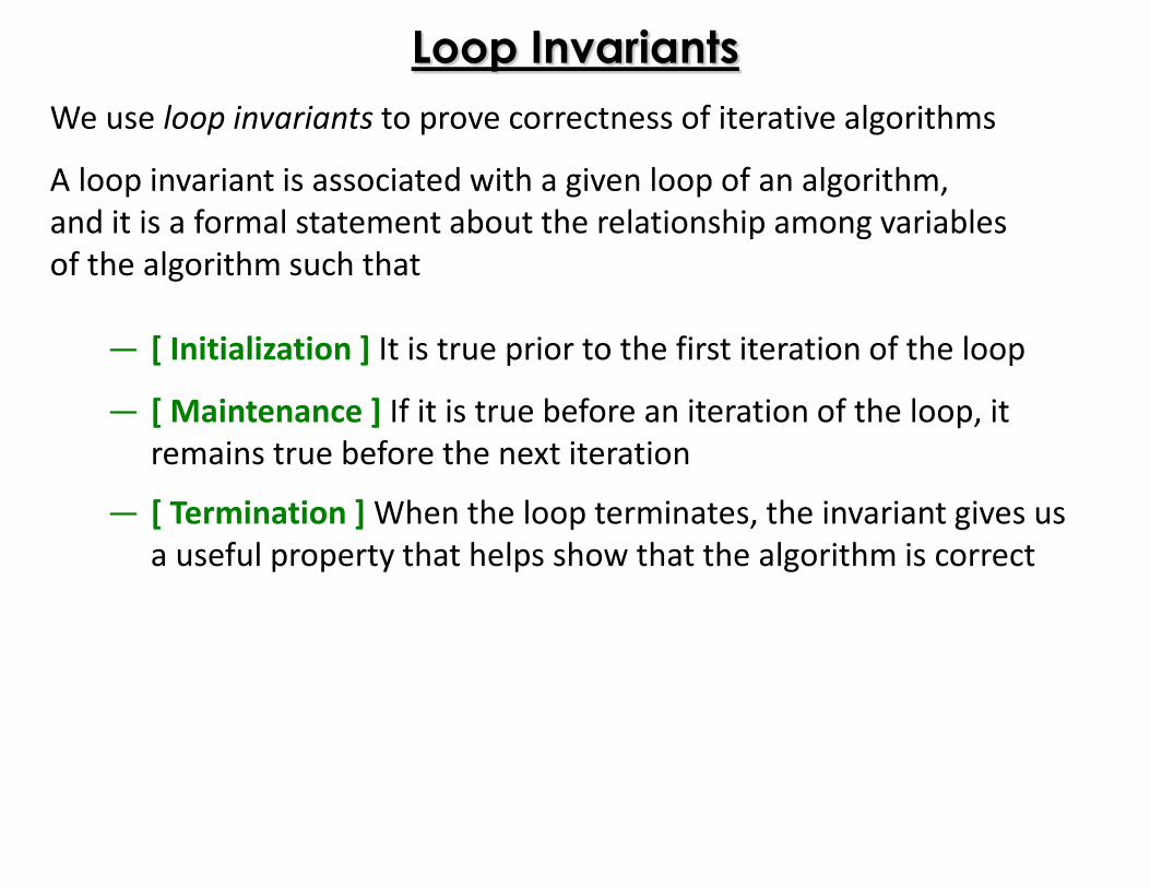
Loop Invariants
We use loop invariants to prove correctness of iterative algorithms
A loop invariant is associated with a given loop of an algorithm,
and it is a formal statement about the relationship among variables
of the algorithm such that
― [ Initialization ] It is true prior to the first iteration of the loop
― [ Maintenance ] If it is true before an iteration of the loop, it
remains true before the next iteration
― [ Termination ] When the loop terminates, the invariant gives us
a useful property that helps show that the algorithm is correct

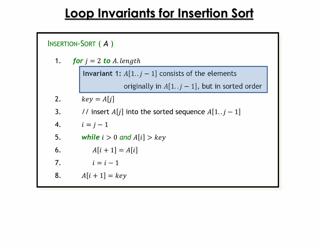
Loop Invariants for Insertion Sort
INSERTION-SORT ( A )
1. for � 2 to �. � ����2. � � � �3. // insert � � into the sorted sequence � 1. . � � 14. � � � 15. while � � 0 and � � � � �6. � � � 1 � �7. � � � 18. � � � 1 � �
Loop Invariants for Insertion Sort
INSERTION-SORT ( A )
1. for � 2 to �. � ����Invariant 1: � 1. . � � 1 consists of the elements
originally in � 1. . � � 1 , but in sorted order
2. � � � �3. // insert � � into the sorted sequence � 1. . � � 14. � � � 15. while � � 0 and � � � � �6. � � � 1 � �7. � � � 18. � � � 1 � �
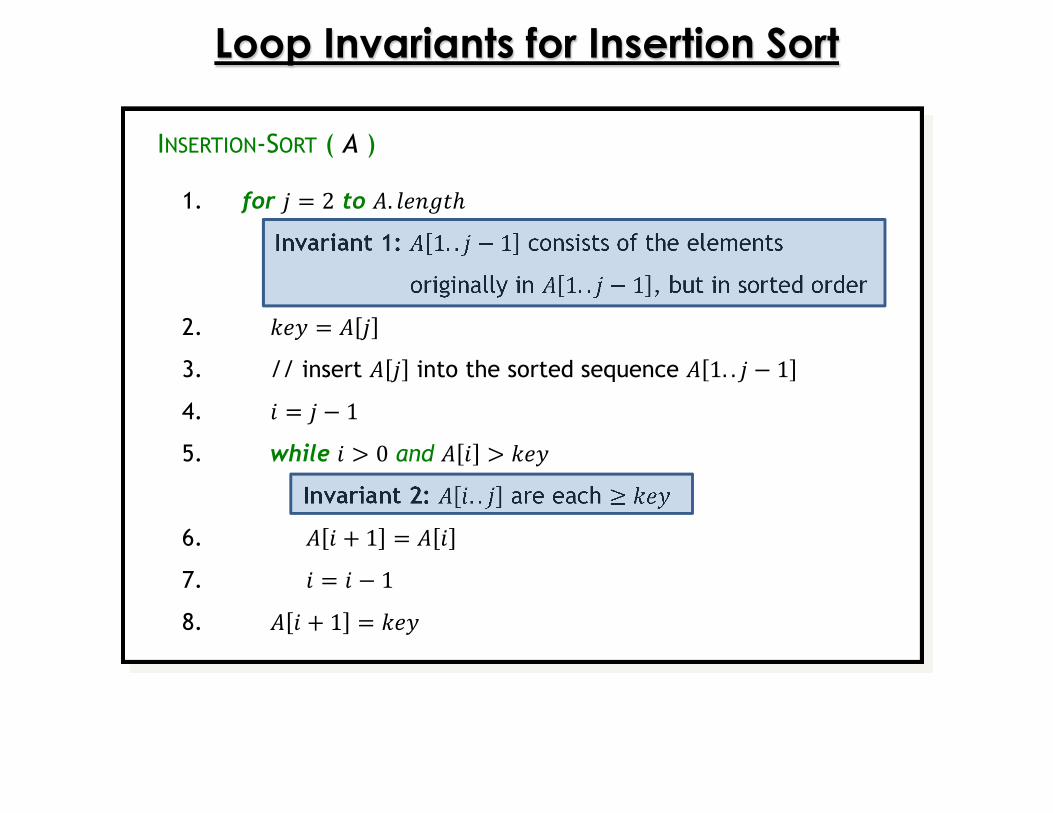
Loop Invariants for Insertion Sort
INSERTION-SORT ( A )
1. for � 2 to �. � ����Invariant 1: � 1. . � � 1 consists of the elements
originally in � 1. . � � 1 , but in sorted order
2. � � � �3. // insert � � into the sorted sequence � 1. . � � 14. � � � 15. while � � 0 and � � � � �
Invariant 2: � �. . � are each � � �6. � � � 1 � �7. � � � 18. � � � 1 � �
Loop Invariant 1: Initialization
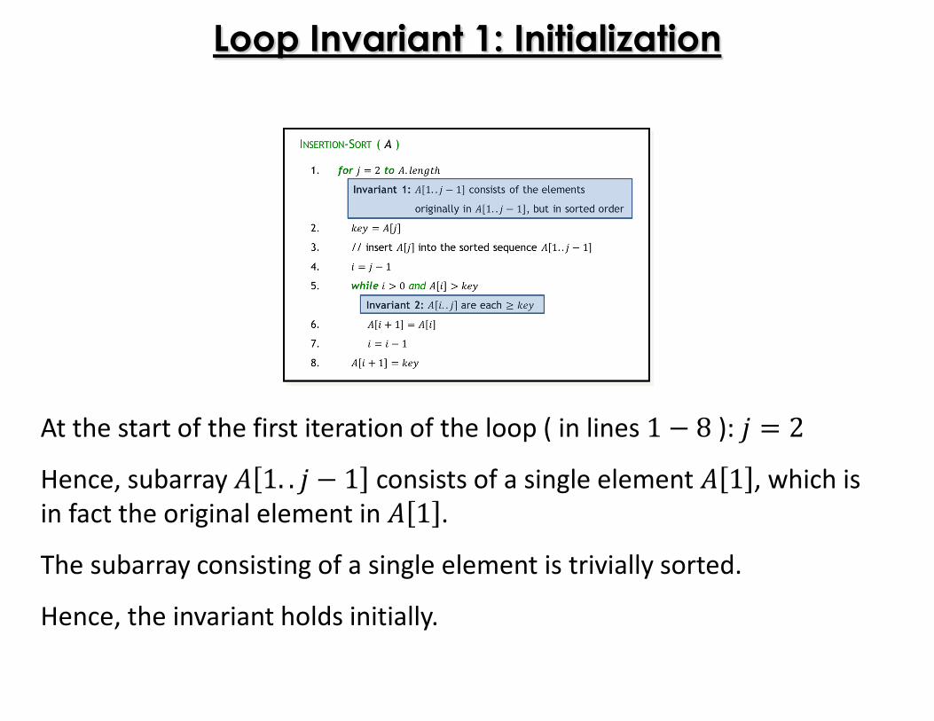
At the start of the first iteration of the loop ( in lines 1 � 8 ): � 2Hence, subarray � 1. . � � 1 consists of a single element � 1 , which is
in fact the original element in � 1 .
The subarray consisting of a single element is trivially sorted.
Hence, the invariant holds initially.
Loop Invariant 1: Maintenance
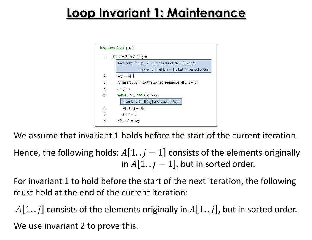
We assume that invariant 1 holds before the start of the current iteration.
Hence, the following holds: � 1. . � � 1 consists of the elements originally
in � 1. . � � 1 , but in sorted order.
For invariant 1 to hold before the start of the next iteration, the following
must hold at the end of the current iteration:� 1. . � consists of the elements originally in � 1. . � , but in sorted order.
We use invariant 2 to prove this.
Loop Invariant 1: MaintenanceLoop Invariant 2: Initialization
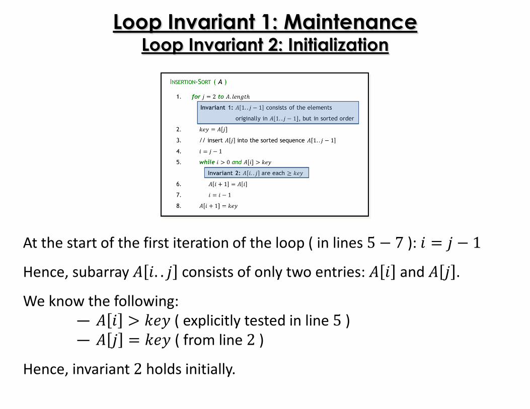
At the start of the first iteration of the loop ( in lines 5 � 7 ): � � � 1Hence, subarray � �. . � consists of only two entries: � � and � � .
We know the following:
― � � � � � ( explicitly tested in line 5 )
― � � � � ( from line 2 )
Hence, invariant 2 holds initially.
Loop Invariant 1: MaintenanceLoop Invariant 2: Maintenance
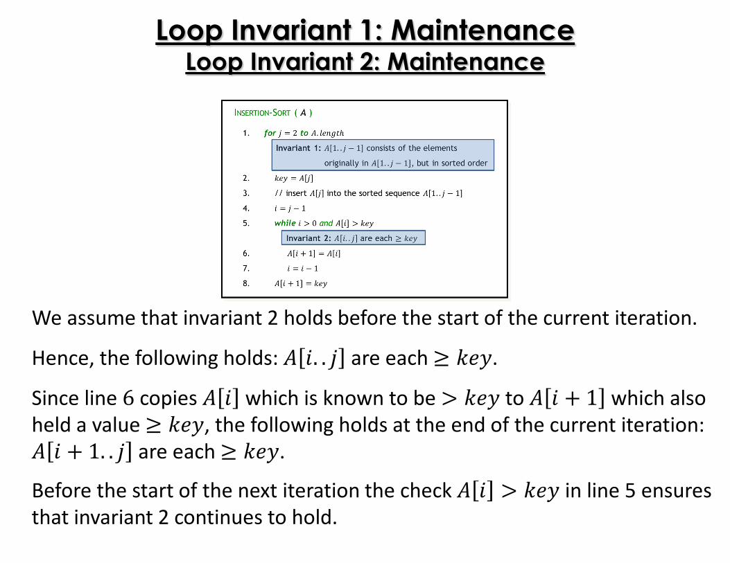
We assume that invariant 2 holds before the start of the current iteration.
Hence, the following holds: � �. . � are each � � �.
Since line 6 copies � � which is known to be � � � to � � � 1 which also
held a value � � �, the following holds at the end of the current iteration: � � � 1. . � are each � � �.
Before the start of the next iteration the check � � � � � in line 5 ensures
that invariant 2 continues to hold.
Loop Invariant 1: MaintenanceLoop Invariant 2: Maintenance
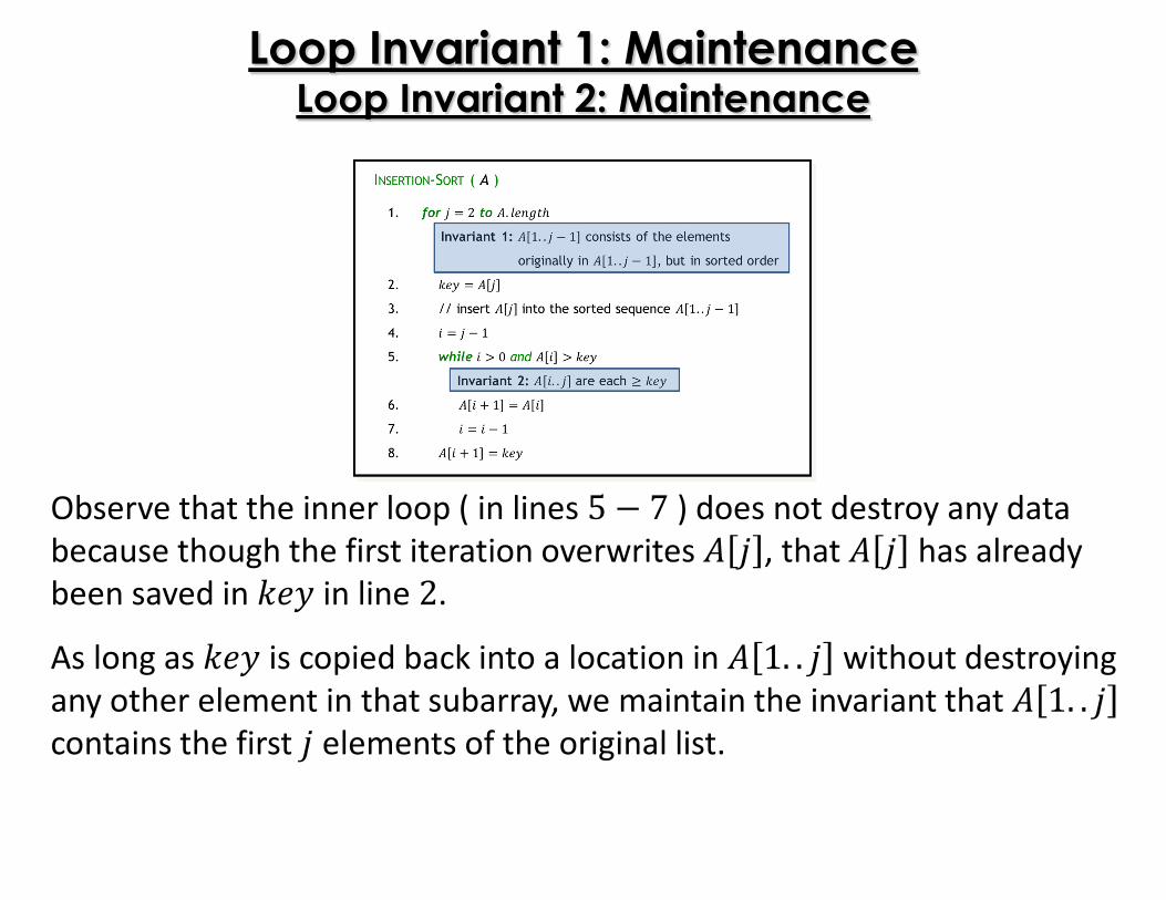
Observe that the inner loop ( in lines 5 � 7 ) does not destroy any data
because though the first iteration overwrites � � , that � � has already
been saved in � � in line 2.
As long as � � is copied back into a location in � 1. . � without destroying
any other element in that subarray, we maintain the invariant that � 1. . �contains the first � elements of the original list.
Loop Invariant 1: MaintenanceLoop Invariant 2: Termination
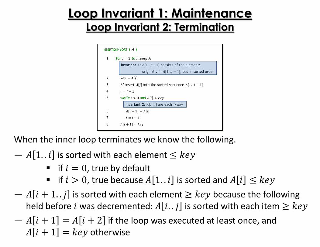
When the inner loop terminates we know the following.
― � 1. . � is sorted with each element � � �� if � 0, true by default
� if � � 0, true because � 1. . � is sorted and � � � � �― � � � 1. . � is sorted with each element � � � because the following
held before � was decremented: � �. . � is sorted with each item � � �― � � � 1 � � � 2 if the loop was executed at least once, and � � � 1 � � otherwise
Loop Invariant 1: MaintenanceLoop Invariant 2: Termination
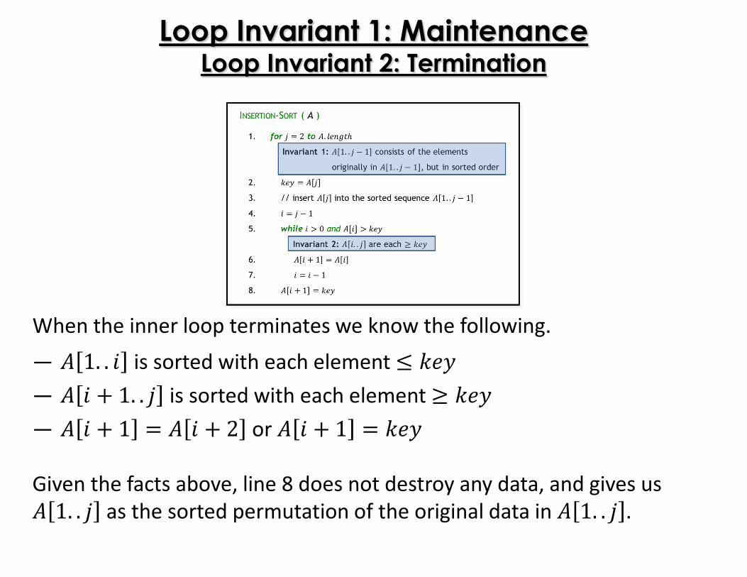
When the inner loop terminates we know the following.
― � 1. . � is sorted with each element � � �― � � � 1. . � is sorted with each element � � �― � � � 1 � � � 2 or � � � 1 � �Given the facts above, line 8 does not destroy any data, and gives us � 1. . � as the sorted permutation of the original data in � 1. . � .
Loop Invariant 1: Termination
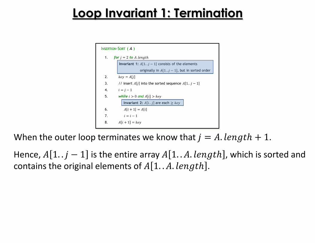
When the outer loop terminates we know that � �. � ���� � 1.
Hence, � 1. . � � 1 is the entire array � 1. . �. � ���� , which is sorted and
contains the original elements of � 1. . �. � ���� .
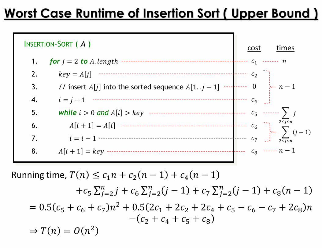
Worst Case Runtime of Insertion Sort ( Upper Bound )
INSERTION-SORT ( A )
1. for � 2 to �. � ����2. � � � �3. // insert � � into the sorted sequence � 1. . � � 14. � � � 15. while � � 0 and � � � � �6. � � � 1 � �7. � � � 18. � � � 1 � �
��� 0�!�"�#�$�%
�� � 1& � '(')& � � 1 '(')� � 1
cost times
Running time, * � � ��� � � � � 1 � �! � � 1��"∑ �)(, � �#∑ � � 1)(, � �$∑ � � 1)(, � �% � � 1 0.5 �" � �# � �$ � � 0.5 2�� � 2� � 2�! � �" � �# � �$ � 2�% �� � � �! � �" � �%⇒ * � . �
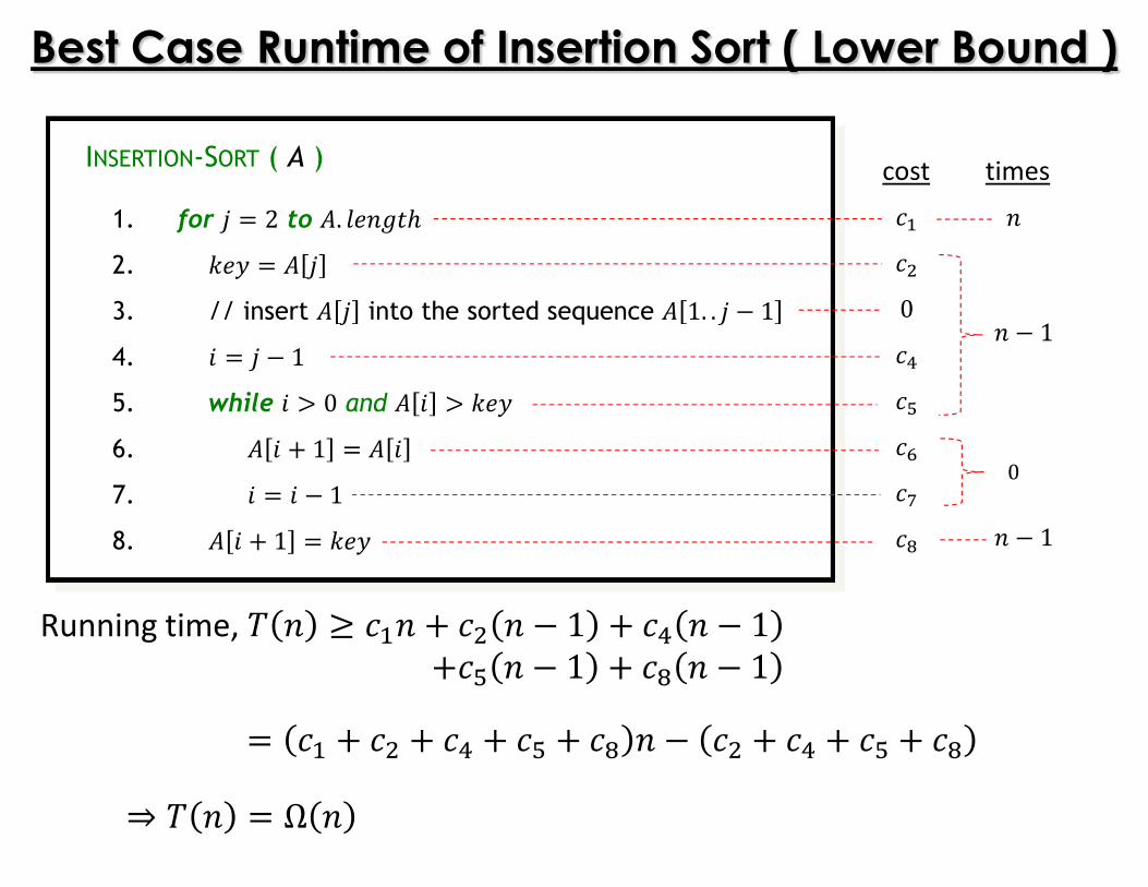
Best Case Runtime of Insertion Sort ( Lower Bound )
INSERTION-SORT ( A )
1. for � 2 to �. � ����2. � � � �3. // insert � � into the sorted sequence � 1. . � � 14. � � � 15. while � � 0 and � � � � �6. � � � 1 � �7. � � � 18. � � � 1 � �
��� 0�!�"�#�$�%
�� � 1
0� � 1
cost times
Running time, * � � ��� � � � � 1 � �! � � 1��" � � 1 � �% � � 1 �� � � � �! � �" � �% � � � � �! � �" � �%
⇒ * � Ω �
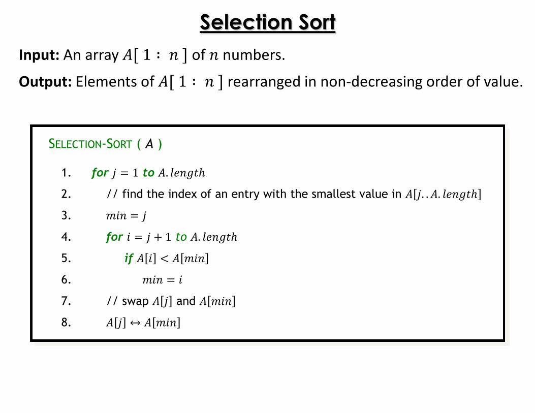
Selection Sort
Input: An array ��1 ∶ �� of � numbers.
Output: Elements of ��1 ∶ �� rearranged in non-decreasing order of value.
SELECTION-SORT ( A )
1. for � 1 to �. � ����2. // find the index of an entry with the smallest value in � �. . �. � ����3. 0�� �4. for � � � 1 to �. � ����5. if � � 1 � 0��6. 0�� �7. // swap � � and � 0��8. � � ↔ � 0��
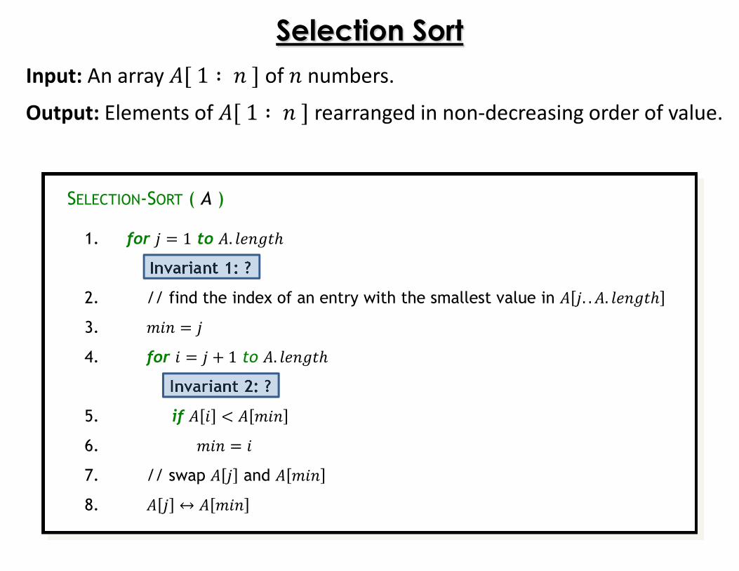
Selection Sort
Input: An array ��1 ∶ �� of � numbers.
Output: Elements of ��1 ∶ �� rearranged in non-decreasing order of value.
SELECTION-SORT ( A )
1. for � 1 to �. � ����Invariant 1: ?
2. // find the index of an entry with the smallest value in � �. . �. � ����3. 0�� �4. for � � � 1 to �. � ����
Invariant 2: ?
5. if � � 1 � 0��6. 0�� �7. // swap � � and � 0��8. � � ↔ � 0��
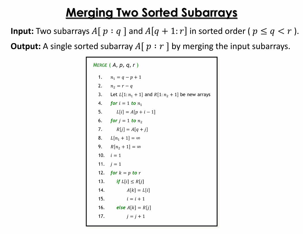
Merging Two Sorted Subarrays
Input: Two subarrays ��3 ∶ 4� and � 4 � 1: 6 in sorted order ( 3 � 4 1 6 ).
Output: A single sorted subarray ��3 ∶ 6� by merging the input subarrays.
Merging Two Sorted Subarrays
Input: Two subarrays ��3 ∶ 4� and � 4 � 1: 6 in sorted order ( 3 � 4 1 6 ).
Output: A single sorted subarray ��3 ∶ 6� by merging the input subarrays.
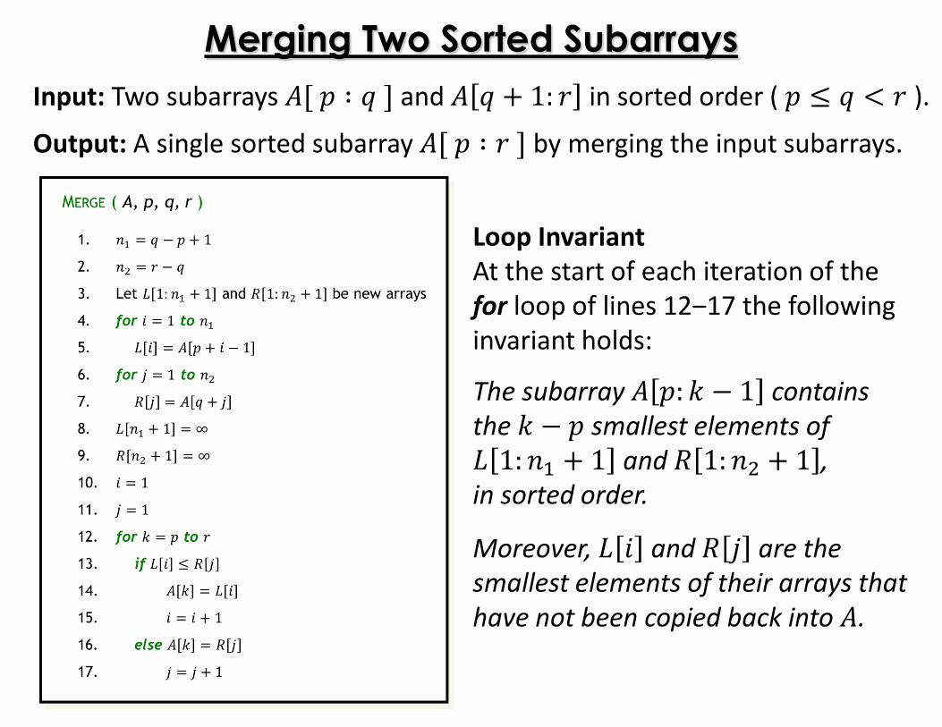
Loop Invariant
At the start of each iteration of the
for loop of lines 12‒17 the following
invariant holds:
The subarray � 3: � � 1 contains
the � � 3 smallest elements of 7 1: �� � 1 and 8 1: � � 1 ,
in sorted order.
Moreover, 7 � and 8 � are the
smallest elements of their arrays that
have not been copied back into �.
Merging Two Sorted Subarrays
Input: Two subarrays ��3 ∶ 4� and � 4 � 1: 6 in sorted order ( 3 � 4 1 6 ).
Output: A single sorted subarray ��3 ∶ 6� by merging the input subarrays.
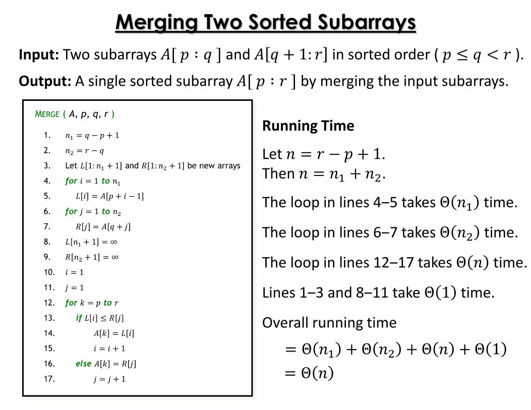
Running Time
Let � 6 � 3 � 1.
Then � �� � � .
The loop in lines 4‒5 takes Θ �� time.
The loop in lines 6‒7 takes Θ � time.
The loop in lines 12‒17 takes Θ � time.
Lines 1‒3 and 8‒11 take Θ 1 time.
Overall running time Θ �� � Θ � � Θ � � Θ 1 Θ �
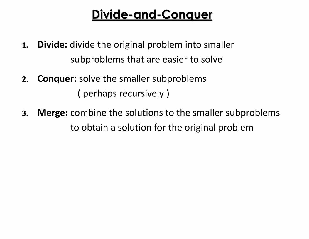
Divide-and-Conquer
1. Divide: divide the original problem into smaller
subproblems that are easier to solve
2. Conquer: solve the smaller subproblems
( perhaps recursively )
3. Merge: combine the solutions to the smaller subproblems
to obtain a solution for the original problem
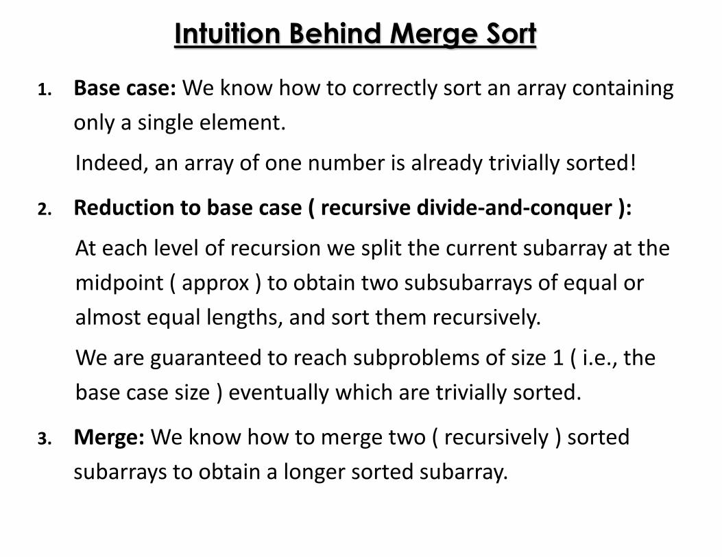
Intuition Behind Merge Sort
1. Base case: We know how to correctly sort an array containing
only a single element.
Indeed, an array of one number is already trivially sorted!
2. Reduction to base case ( recursive divide-and-conquer ):
At each level of recursion we split the current subarray at the
midpoint ( approx ) to obtain two subsubarrays of equal or
almost equal lengths, and sort them recursively.
We are guaranteed to reach subproblems of size 1 ( i.e., the
base case size ) eventually which are trivially sorted.
3. Merge: We know how to merge two ( recursively ) sorted
subarrays to obtain a longer sorted subarray.
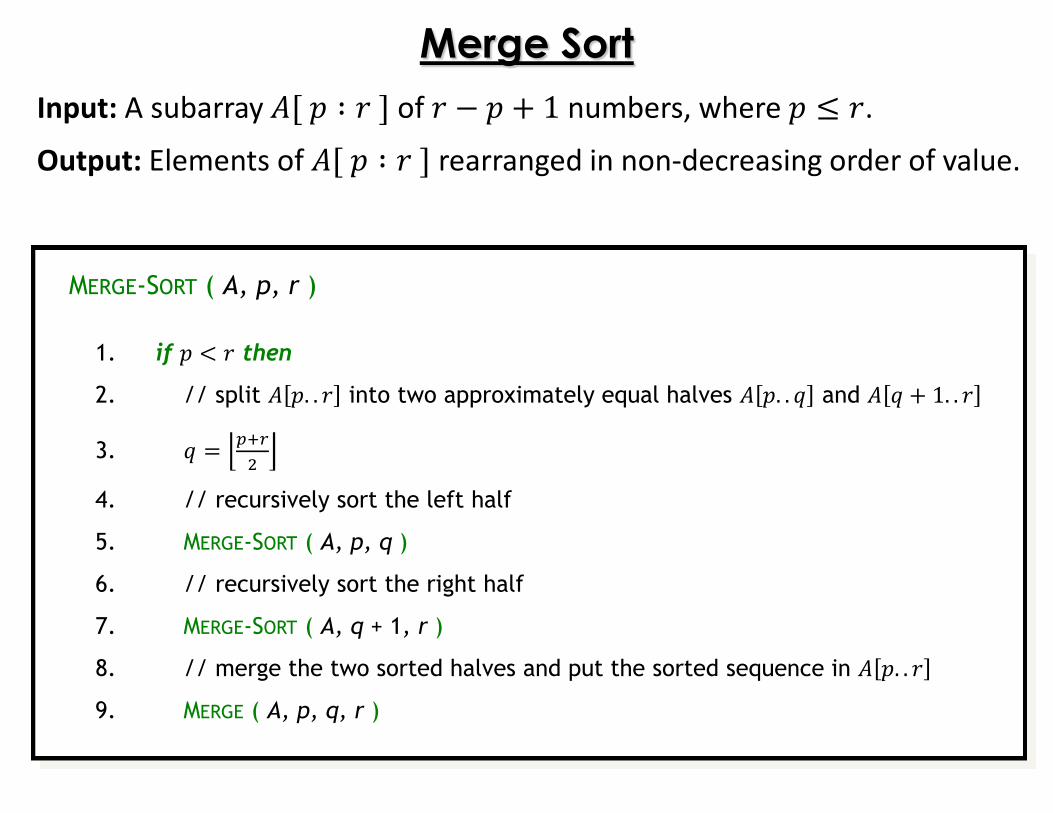
Merge Sort
Input: A subarray ��3 ∶ 6� of 6 � 3 � 1 numbers, where 3 � 6.
Output: Elements of ��3 ∶ 6� rearranged in non-decreasing order of value.
MERGE-SORT ( A, p, r )
1. if 3 1 6 then
2. // split � 3. . 6 into two approximately equal halves � 3. . 4 and � 4 � 1. . 63. 4 :;< 4. // recursively sort the left half
5. MERGE-SORT ( A, p, q )
6. // recursively sort the right half
7. MERGE-SORT ( A, q + 1, r )
8. // merge the two sorted halves and put the sorted sequence in � 3. . 69. MERGE ( A, p, q, r )
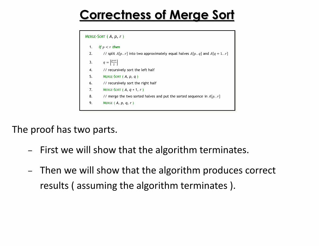
Correctness of Merge Sort
The proof has two parts.
‒ First we will show that the algorithm terminates.
‒ Then we will show that the algorithm produces correct
results ( assuming the algorithm terminates ).
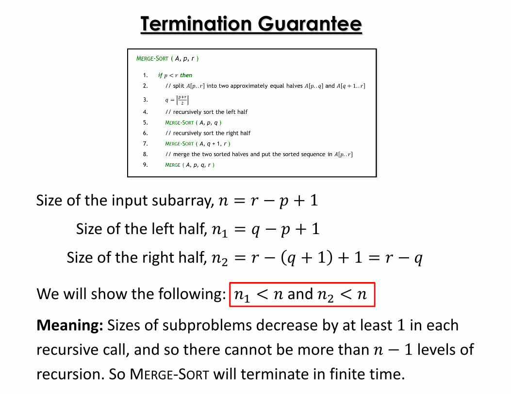
Termination Guarantee
Size of the input subarray, � 6 � 3 � 1Size of the left half, �� 4 � 3 � 1
Size of the right half, � 6 � 4 � 1 � 1 6 � 4We will show the following: �� 1 � and � 1 �Meaning: Sizes of subproblems decrease by at least 1 in each
recursive call, and so there cannot be more than � � 1 levels of
recursion. So MERGE-SORT will terminate in finite time.
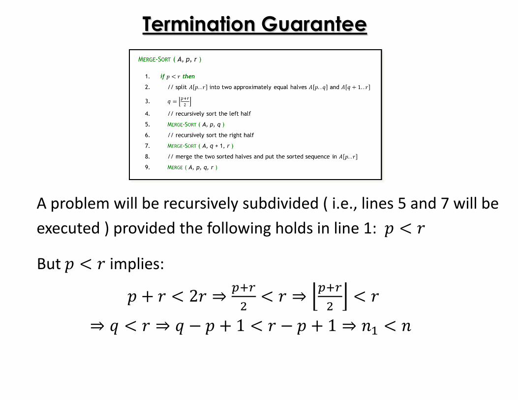
Termination Guarantee
A problem will be recursively subdivided ( i.e., lines 5 and 7 will be
executed ) provided the following holds in line 1: 3 1 6But 3 1 6 implies:
3 � 6 1 26 ⇒ :;< 1 6 ⇒ :;< 1 6⇒ 4 1 6 ⇒ 4 � 3 � 1 1 6 � 3 � 1 ⇒ �� 1 �
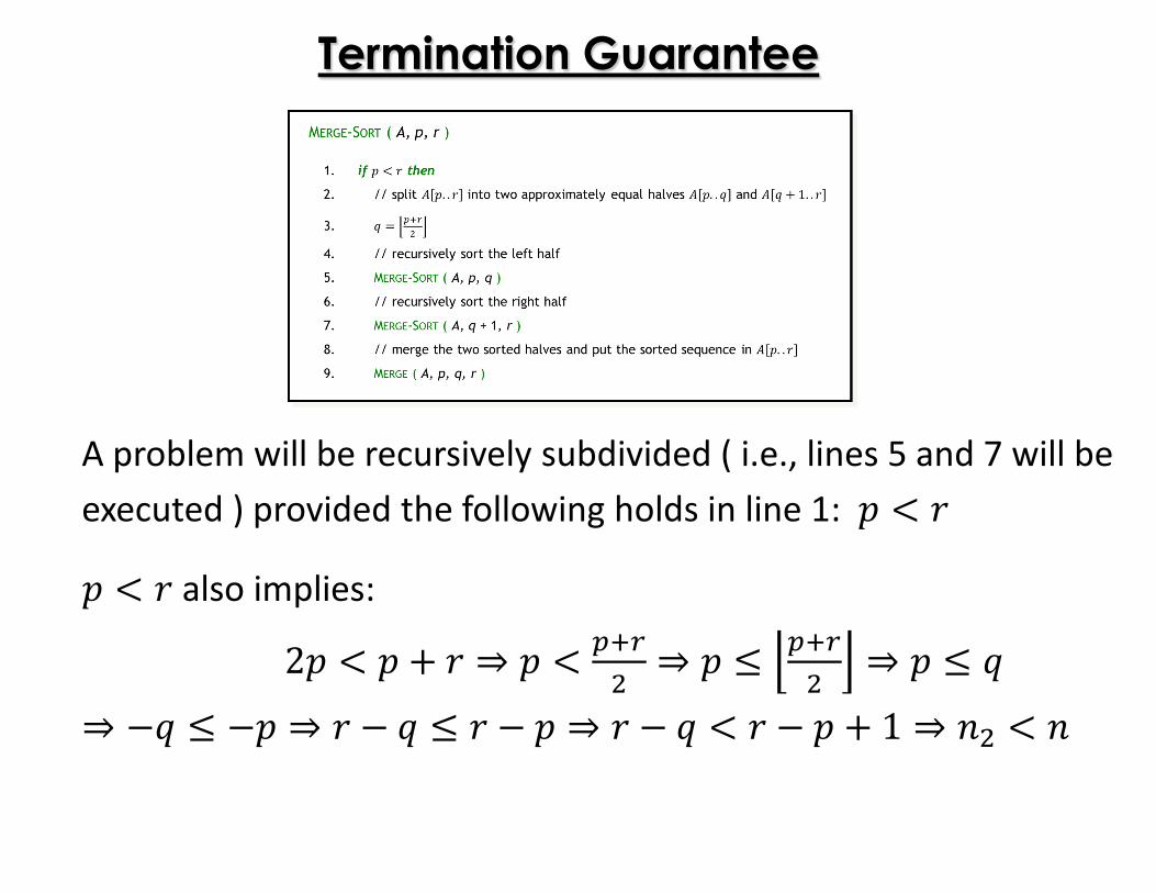
Termination Guarantee
A problem will be recursively subdivided ( i.e., lines 5 and 7 will be
executed ) provided the following holds in line 1: 3 1 63 1 6 also implies:
23 1 3 � 6 ⇒ 3 1 :;< ⇒ 3 � :;< ⇒ 3 � 4⇒ �4 � �3 ⇒ 6 � 4 � 6 � 3 ⇒ 6 � 4 1 6 � 3 � 1 ⇒ � 1 �
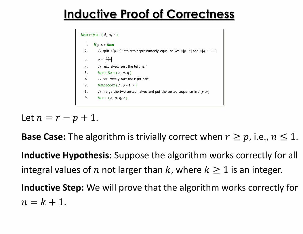
Inductive Proof of Correctness
Base Case: The algorithm is trivially correct when 6 � 3, i.e., � � 1.
Let � 6 � 3 � 1.
Inductive Hypothesis: Suppose the algorithm works correctly for all
integral values of � not larger than �, where � � 1 is an integer.
Inductive Step: We will prove that the algorithm works correctly for � � � 1.
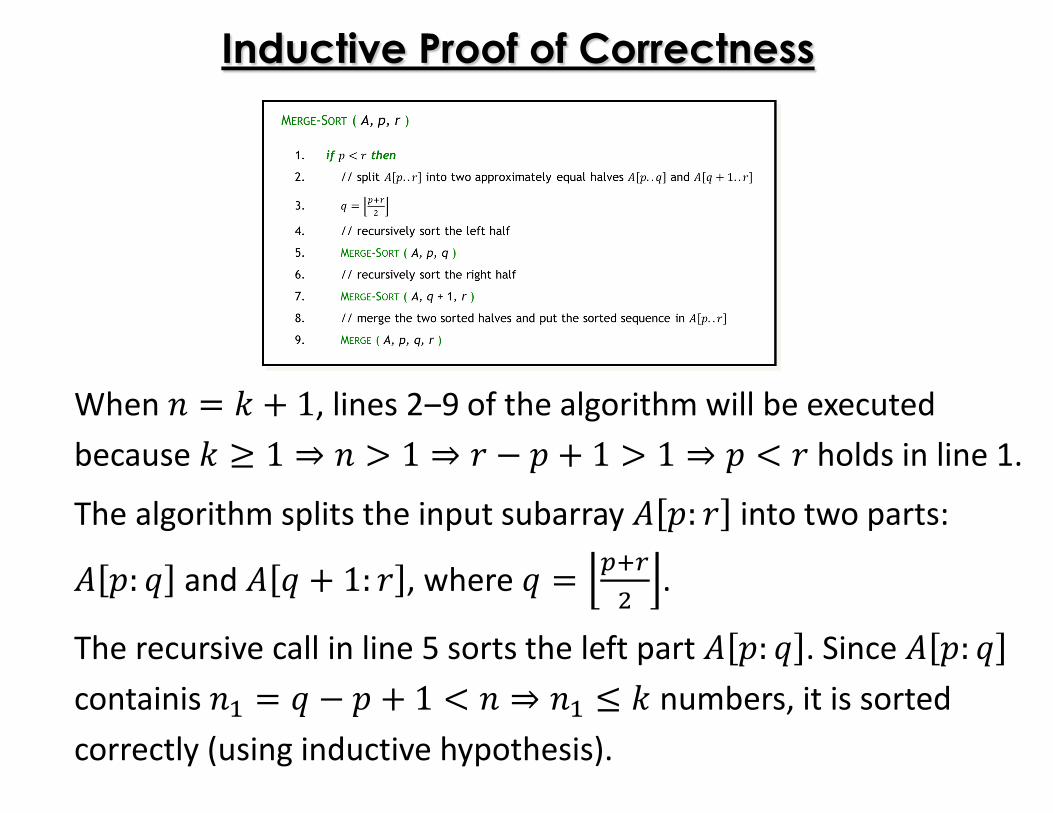
Inductive Proof of Correctness
When � � � 1, lines 2‒9 of the algorithm will be executed
because � � 1 ⇒ � � 1 ⇒ 6 � 3 � 1 � 1 ⇒ 3 1 6 holds in line 1.
The algorithm splits the input subarray � 3: 6 into two parts:
� 3: 4 and � 4 � 1: 6 , where 4 :;< .
The recursive call in line 5 sorts the left part � 3: 4 . Since � 3: 4containis �� 4 � 3 � 1 1 � ⇒ �� � � numbers, it is sorted
correctly (using inductive hypothesis).
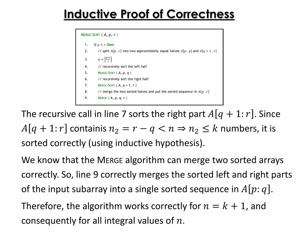
Inductive Proof of Correctness
The recursive call in line 7 sorts the right part � 4 � 1: 6 . Since � 4 � 1: 6 containis � 6 � 4 1 � ⇒ � � � numbers, it is
sorted correctly (using inductive hypothesis).
We know that the MERGE algorithm can merge two sorted arrays
correctly. So, line 9 correctly merges the sorted left and right parts
of the input subarray into a single sorted sequence in � 3: 4 .
Therefore, the algorithm works correctly for � � � 1, and
consequently for all integral values of �.
Analyzing Divide-and-Conquer Algorithms
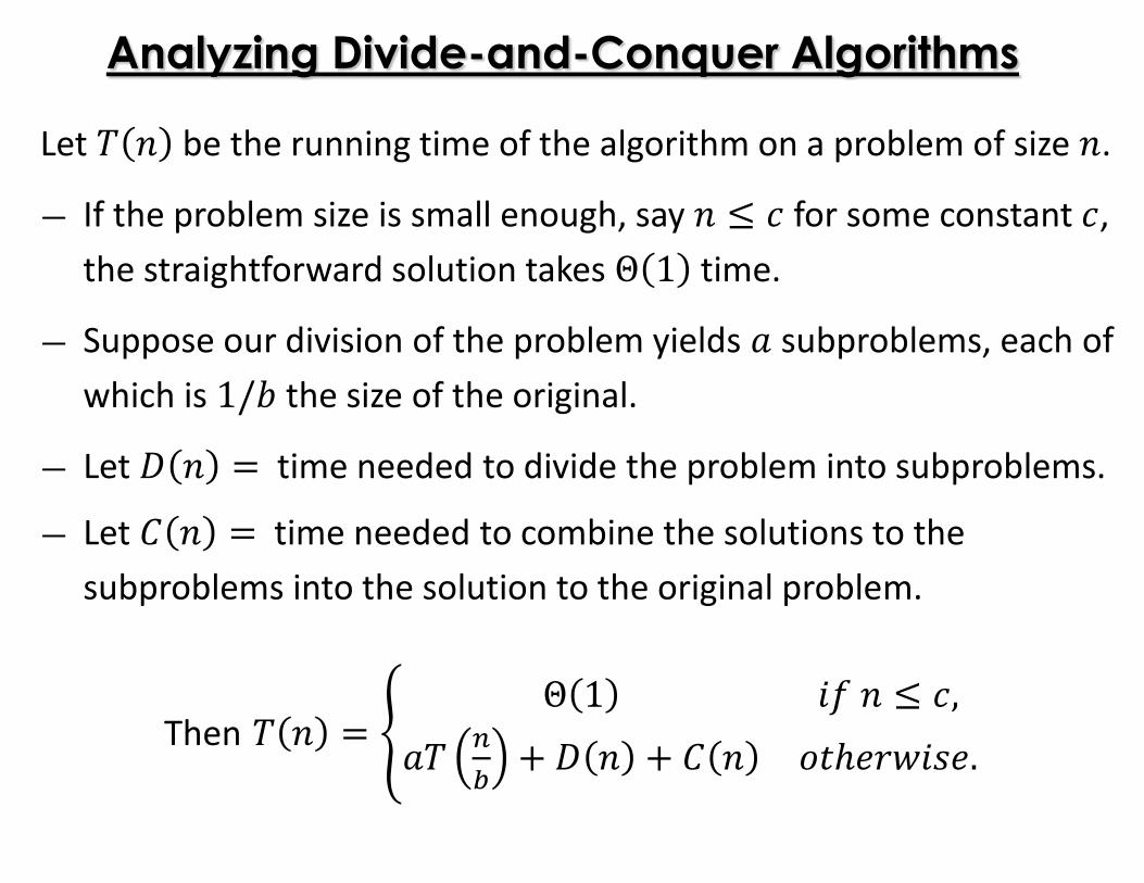
Let * � be the running time of the algorithm on a problem of size �.
― If the problem size is small enough, say � � � for some constant �,
the straightforward solution takes Θ 1 time.
― Suppose our division of the problem yields = subproblems, each of
which is 1/? the size of the original.
― Let @ � time needed to divide the problem into subproblems.
― Let A � time needed to combine the solutions to the
subproblems into the solution to the original problem.
Then * � B Θ 1 �C� � �,=* )E � @ � � A � F�� 6G�H .
Analysis of Merge Sort
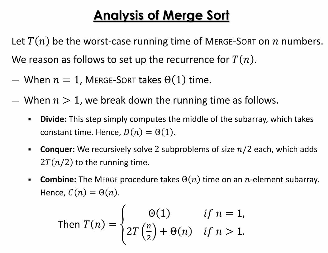
Let * � be the worst-case running time of MERGE-SORT on � numbers.
We reason as follows to set up the recurrence for * � .
― When � 1, MERGE-SORT takes Θ 1 time.
― When � � 1, we break down the running time as follows.
� Divide: This step simply computes the middle of the subarray, which takes
constant time. Hence, @ � Θ 1 .
� Conquer: We recursively solve 2 subproblems of size �/2 each, which adds 2* �/2 to the running time.
� Combine: The MERGE procedure takes Θ � time on an �-element subarray.
Hence, A � Θ � .
Then * � B Θ 1 �C� 1,2* ) � Θ � �C� � 1.
Analysis of Merge Sort
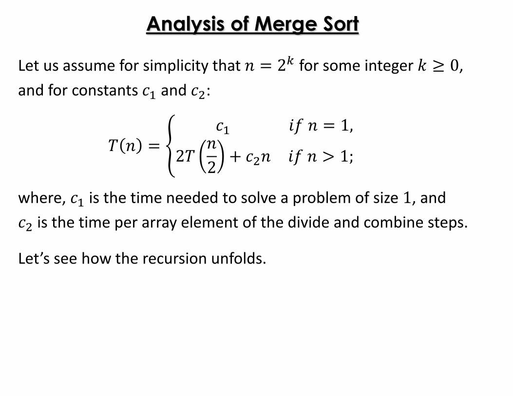
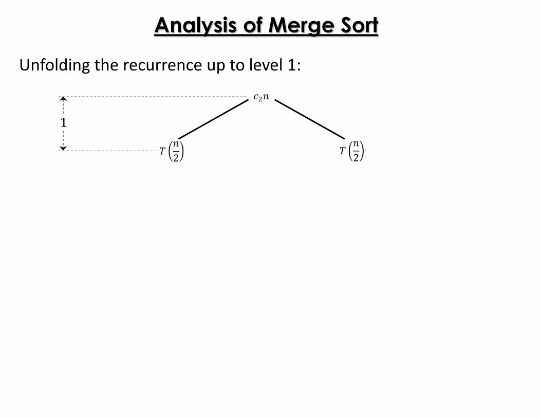
Let us assume for simplicity that � 2I for some integer � � 0,
and for constants �� and � :
* � B �� �C� 1,2* �2 � � � �C� � 1;where, �� is the time needed to solve a problem of size 1, and � is the time per array element of the divide and combine steps.
Let’s see how the recursion unfolds.
Analysis of Merge Sort
* �Running time on an input of size � 2I for some integer � � 0:
Analysis of Merge Sort
� �
* �2 * �21
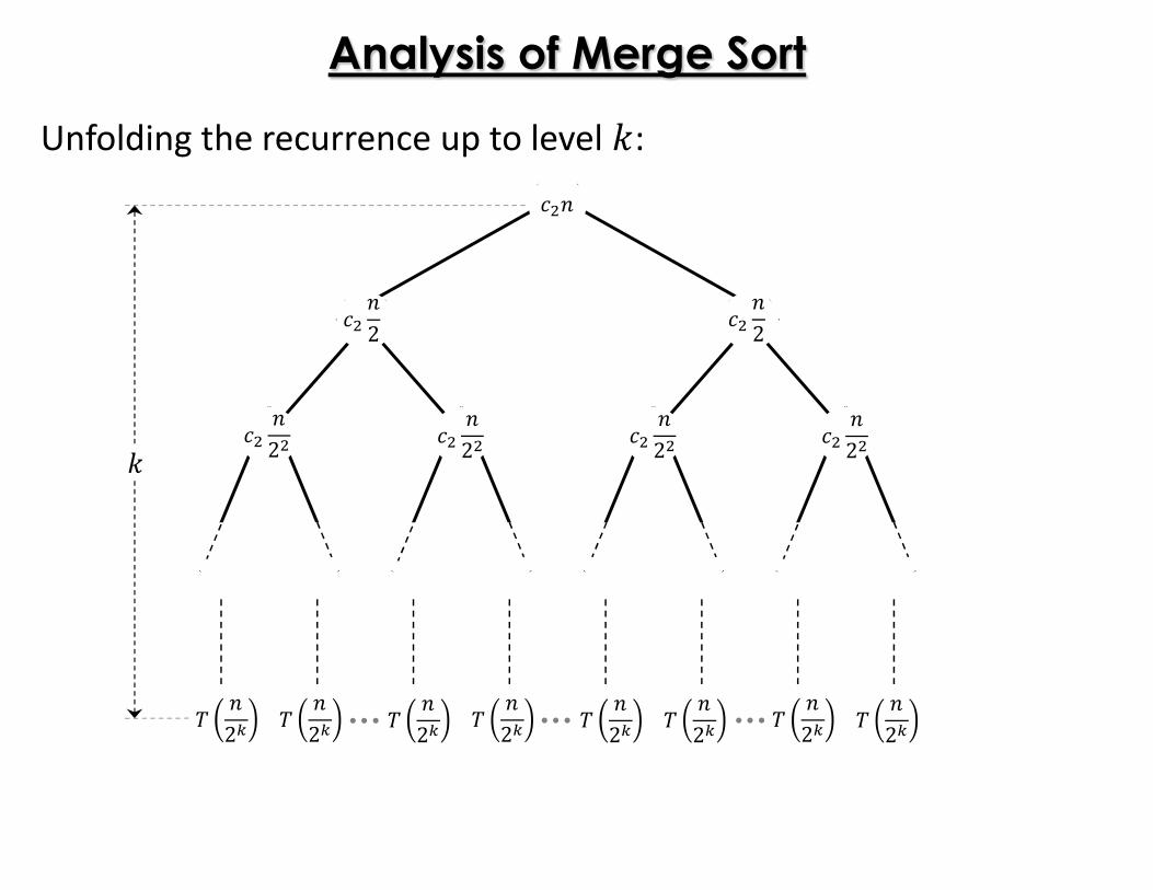
Unfolding the recurrence up to level 1:
Analysis of Merge Sort
� �
� �2 � �2* �2 * �2 * �2 * �2
2
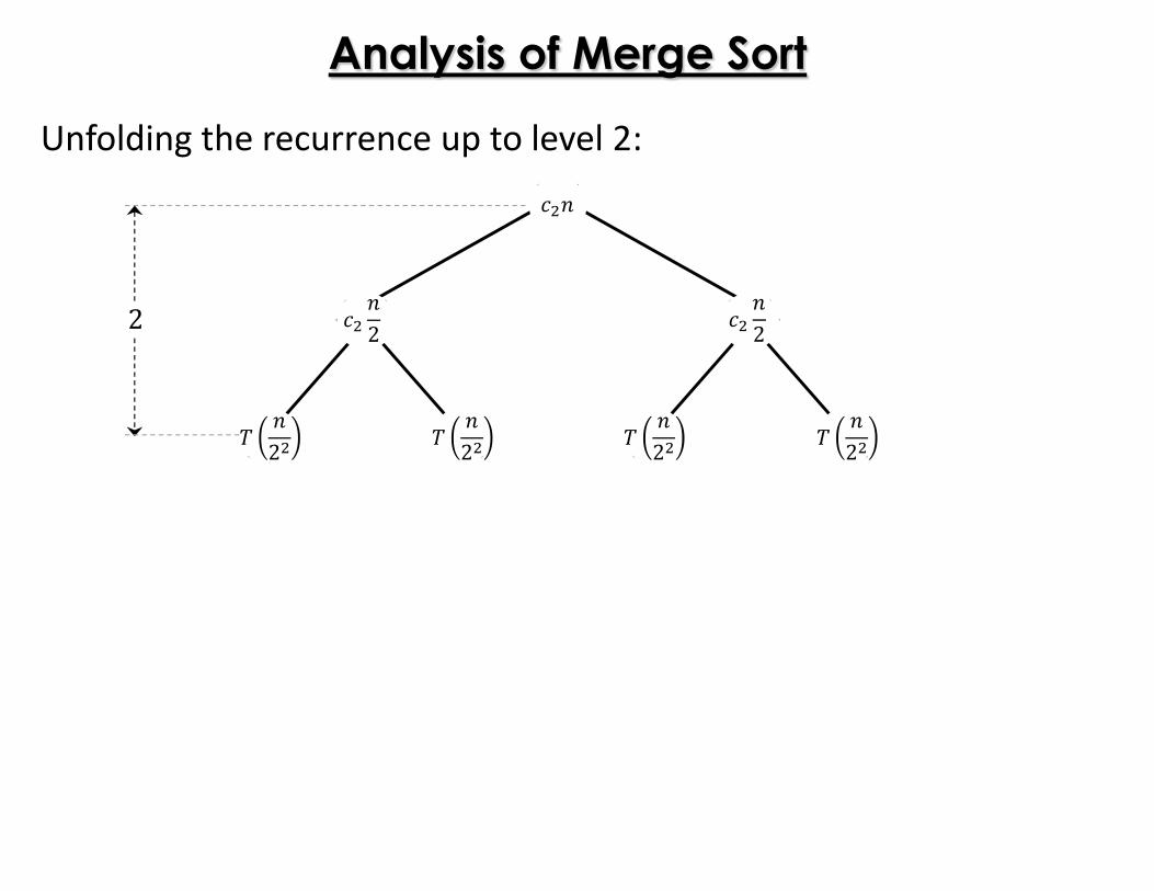
Unfolding the recurrence up to level 2:
Analysis of Merge Sort
� �
� �2 � �2� �2 � �2 � �2 � �2
* �2K * �2K * �2K * �2K * �2K * �2K * �2K * �2K
3
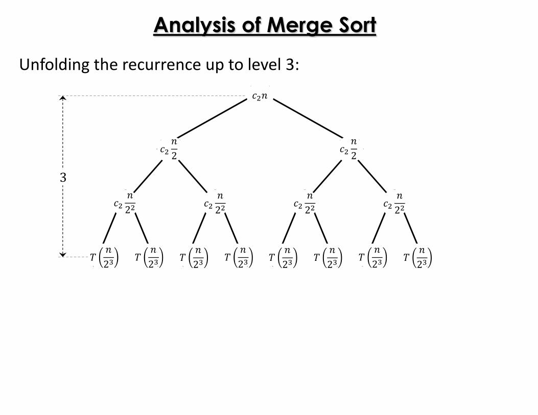
Unfolding the recurrence up to level 3:
Analysis of Merge Sort
� �
� �2 � �2� �2 � �2 � �2 � �2
* �2I * �2I * �2I * �2I * �2I * �2I * �2I * �2I
�
Unfolding the recurrence up to level �:
Analysis of Merge Sort
� �
� �2 � �2� �2 � �2 � �2 � �2 �
* 1 * 1 * 1 * 1 * 1 * 1 * 1 * 1�
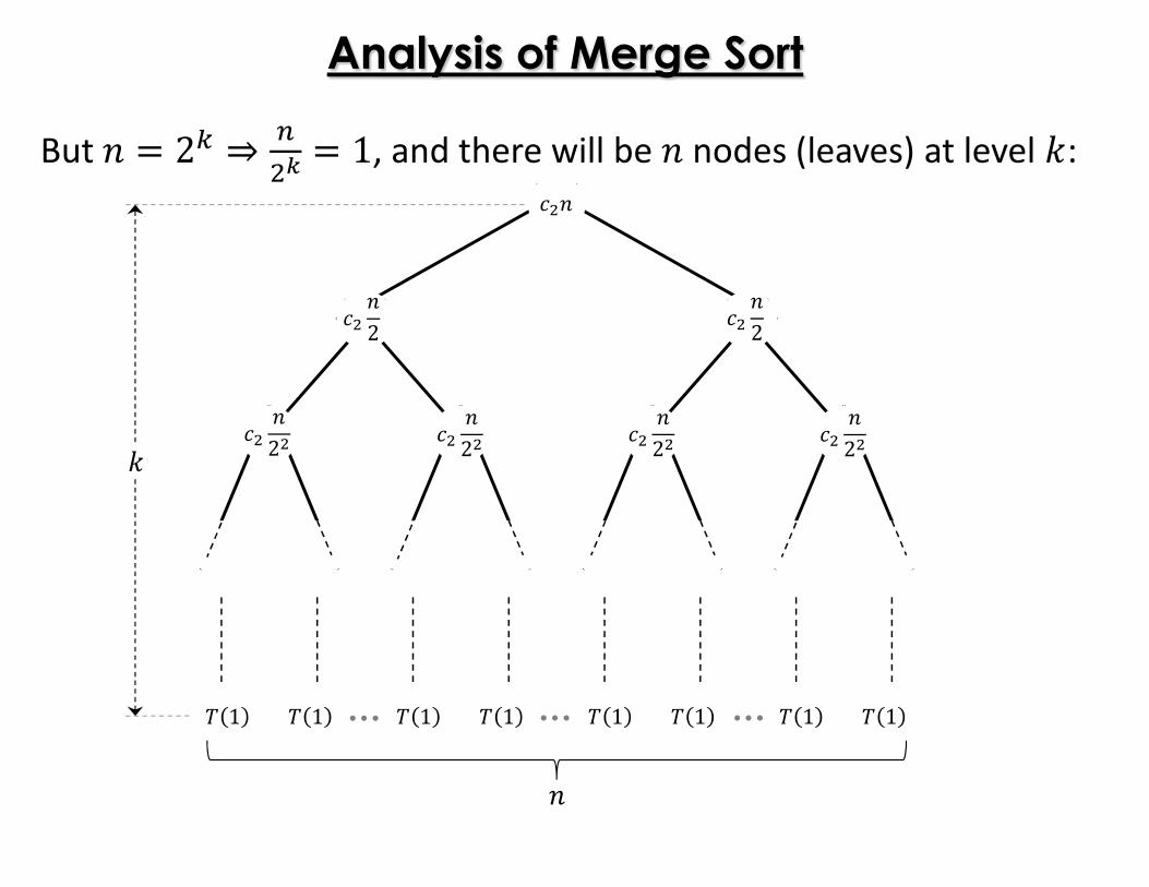
But � 2I ⇒ ) M 1, and there will be � nodes (leaves) at level �:
Analysis of Merge Sort
� �
� �2 � �2� �2 � �2 � �2 � �2 �
��� �� �� �� �� �� �� ��
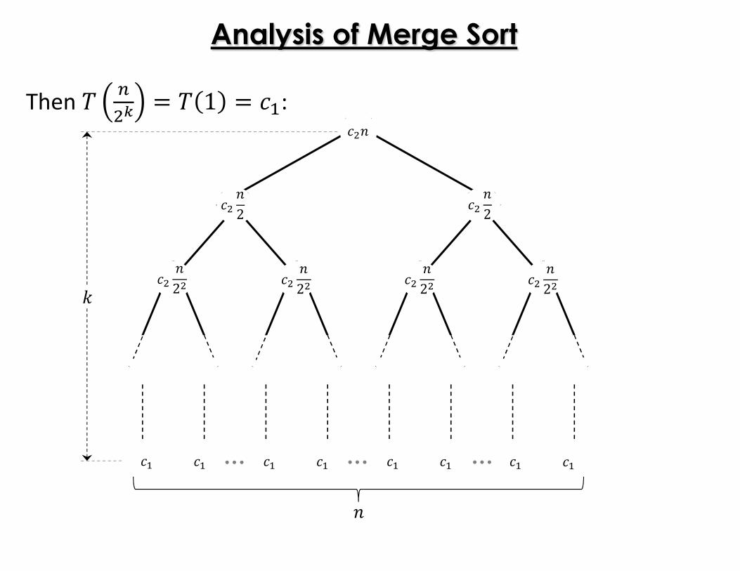
Then * ) M * 1 ��:
Analysis of Merge Sort
� �
� �2 � �2� �2 � �2 � �2 � �2 �
��� �� �� �� �� �� �� ��
� �
� �
� �
���
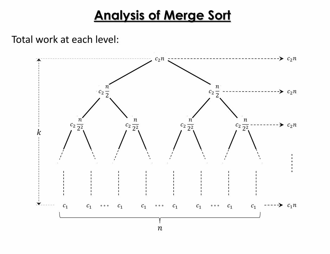
Total work at each level:
Analysis of Merge Sort
� �
� �2 � �2� �2 � �2 � �2 � �2 �
��� �� �� �� �� �� �� ��
� �
� �
� �
���Total: � �� � ���
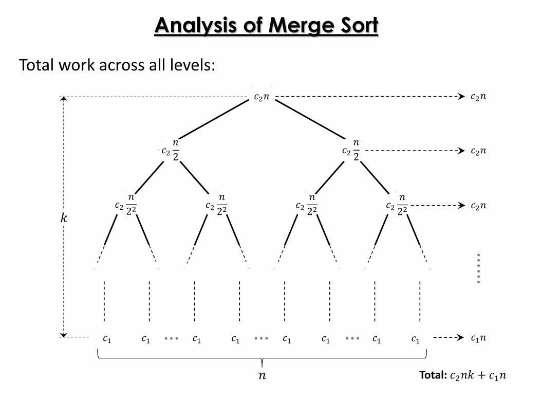
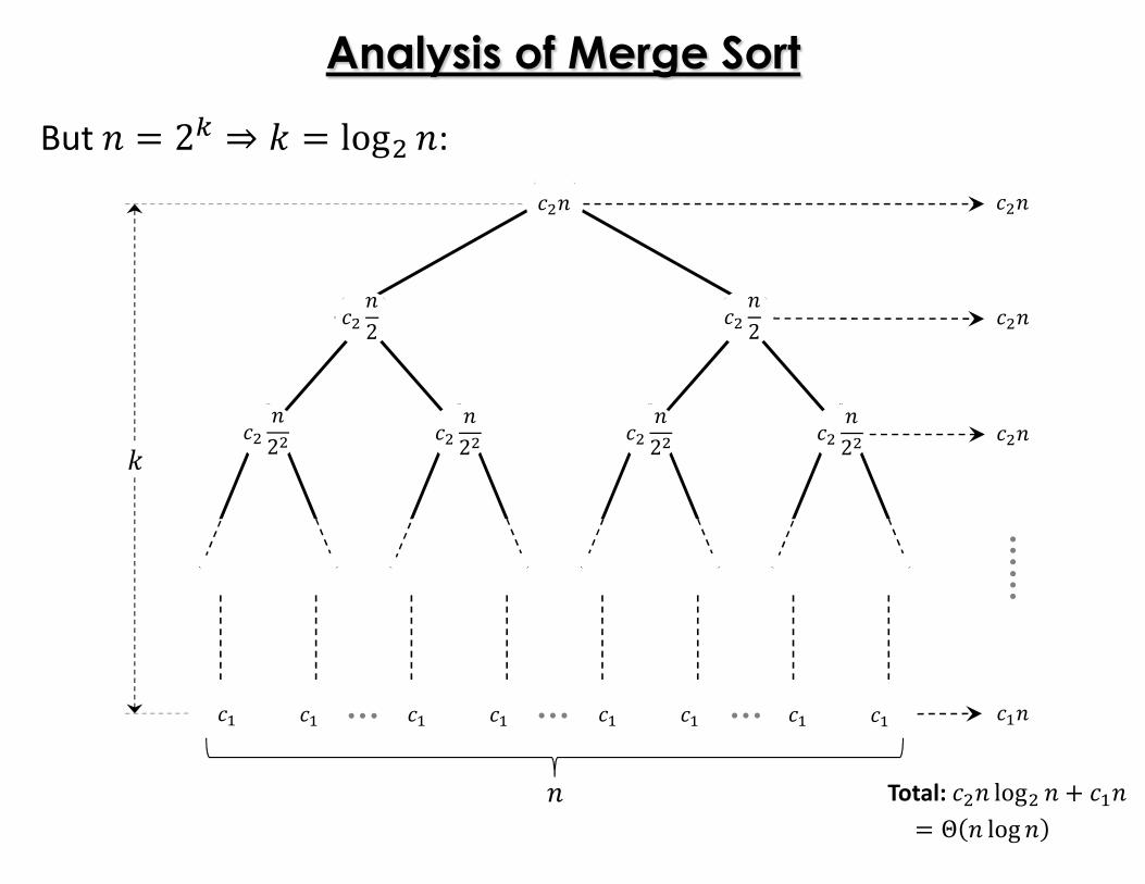
Total work across all levels:
Analysis of Merge Sort
� �
� �2 � �2� �2 � �2 � �2 � �2 �
��� �� �� �� �� �� �� ��
� �
� �
� �
���Total: � � log � � ��� Θ � log�
But � 2I ⇒ � log �:
Related Documents