CSC535: Probabilistic Graphical Models Dynamical Systems Prof. Jason Pacheco ( Some material from Prof. Kobus Barnard)

Welcome message from author
This document is posted to help you gain knowledge. Please leave a comment to let me know what you think about it! Share it to your friends and learn new things together.
Transcript

CSC535: Probabilistic Graphical Models
Dynamical Systems
Prof. Jason Pacheco( Some material from Prof. Kobus Barnard)

Administrivia
• HW3 Extension (tonight @ 11:59pm)
• -10pts per day after that, through Friday
• Monday, Midterm review

Outline
• Sequence Models
• Linear Dynamical Systems
• LDS Extensions

Outline
• Sequence Models
• Linear Dynamical Systems
• LDS Extensions

Much of this section follows Bishop chapter 13
See also Murphy chapters 17 and 18
Sequential data

Sequential data has order, and the order matters.
What has happened, informs what will happen.
Sequential data is everywhere.
Examples:spoken language (word production)written language (sentence level statistics)weatherhuman movementstock market datagenomes
Sequential data

Graphical models for such data?
The complexity of the representation seems to increase with time.
Observations over time tend to depend on the past.
We can simply life by assuming that the distant past does not matter.
If we assume that history does not matter other than the immediate previous entity, we have a first order Markov model.
If what happens now depends on two previous entities, we have a second order Markov model.
Sequential data

First order
Second order
Zeroth order
Markov chains

First order
Second order
Zeroth order
Markov chains
Notice that this plan has arrows from data-thiscomplicates model specification

Hidden Markov Model (HMM)
Intuition Temporal extension of mixture model• Data clusters into hidden “states” Z at each time• Hidden state encodes important part of history• Markov chain models transitions among clusters
Introducing latent state simplifies modeling data likelihood…

Markovian assumptions
The basic HMM is like a mixture model, with the mixture component being used for the current observations depends on the last previous component.
Observation likelihood models how data from a component are generated (things are easy if you know the cluster)

State Transition Diagram(Not a PGM)
Transition Dynamics<—next state —>
current state
Ajk : Probability of going from state j=4 to state
k=3
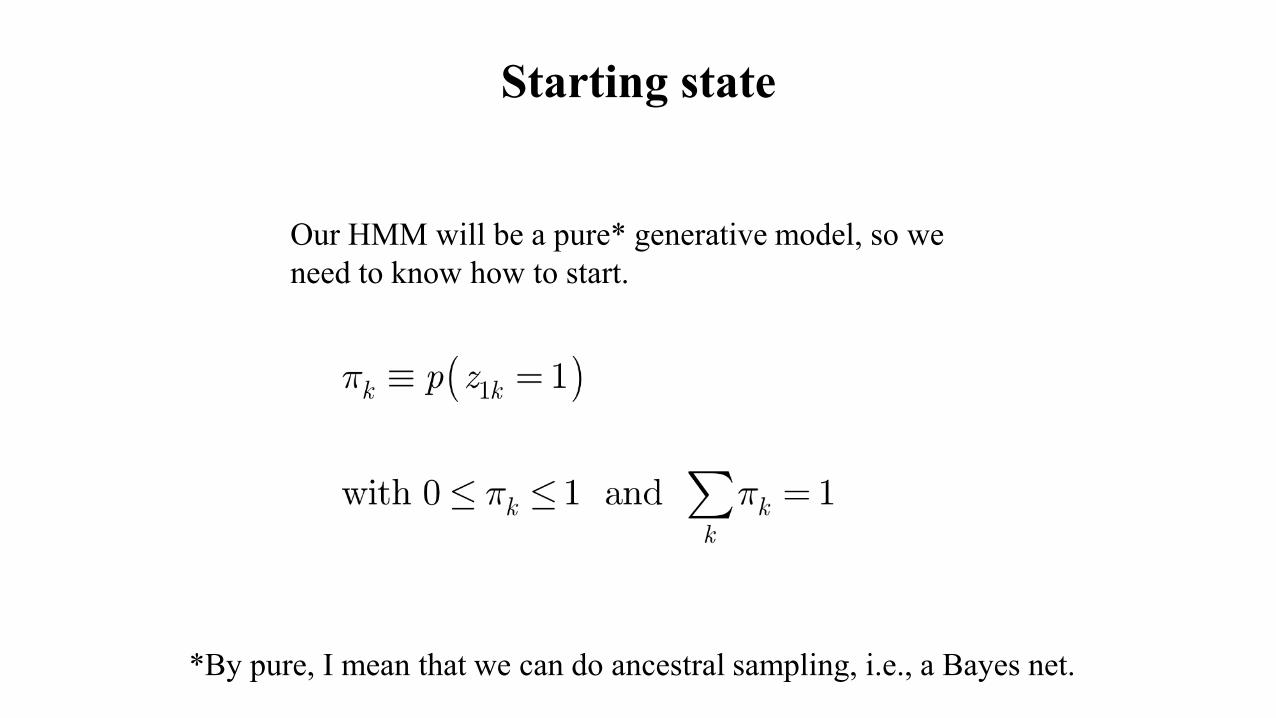
Our HMM will be a pure* generative model, so we need to know how to start.
Starting state
*By pure, I mean that we can do ancestral sampling, i.e., a Bayes net.

HMM parameter summary

Data distribution from an HMM
= ?

Data distribution from an HMM

Data distribution from an HMM

Transition probability to another state is 5% (from Bishop—the short visits in green seem a bit anomalous).
Data distribution from an HMM
Gaussian likelihood model p(xn|zn)
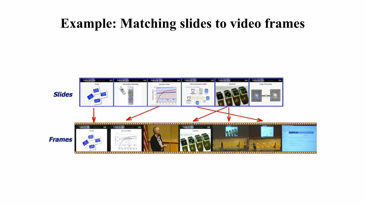
Example: Matching slides to video frames

Our state sequence corresponds to what slide is being shown.
Matching slides to video frames
We assume that only the jump matters. IE, going from slide 6 to 8 has the same chance of going from 10 to 12.

Our state sequence corresponds to what slide is being shown.
Matching slides to video frames
Image matching likelihood

1. Given unlabeled* data, what is the HMM (parameter learning).
2. Given an HMM and observed data, what is the probability distribution of states for each time point (zn in our notation).
3. Given an HMM and observed data, what is the most likely state sequence?
*We could have data with labels (annotated) which means this step becomes trivial, much like training naive Bayes versus fitting a GMM using EM. This is
what we did in the matching slides to video project.
Classic HMM computational problems

1. Given unlabeled* data, what is the HMM (parameter learning).
2. Given an HMM and observed data, what is the probability distribution of states for each time point (zn in our notation).
3. Given an HMM and observed data, what is the most probable state sequence?
Classic HMM computational problems
#2 and #3 seem similar, but to understand the difference consider a three state system about doing HW problems A, B, and C in order, with B being very easy. So you will spend most of your time in state A and C. State B may be the least likely state for every time point. But the most likely state sequence must include it.

Classic HMM computational problems
1. Given unlabeled data, what is the HMM (learning).This is a missing value problem, which we can tackle using EM, but
we will need to solve #2 as sub-problem.
2. Given an HMM and data, what is the probabilitydistribution of states for each time point (zn in our notation).
These are marginals in a Bayes net, and so we use the sum-product algorithm (in HMM often called alpha-beta or forwards backwards).
3. Given an HMM and data, what is the most likely state sequence?
This is a maximal configuration of a Bayes net, and so we use max-sum (in HMM this is Viterbi).

Learning the HMM using EM (Baum-Welch Algorithm)
A natural first “hammer” for HMM is EM because the key issue is our ignorance about the correspondence between data and latent state.
But there are many other ways to do the learning that are less susceptible to local optima (at the expense of CPU time)

Learning the HMM using EM (AKA Baum-Welch)
Bishop chapter 13 only considers earning from one sequence.
Often you have many shorter sequences, and extending to multiple training sequences is easy (so we will do that).
Depending on what you want your model to do, the prior over initial state is the overall prior (you can jump in anywhere) or it really matters where you start.
I will extend Bishop’s notation to have E training sequence examples (or experiments) indexed by e, with each sequence having Ne points*, and we will assume where start matters.
*It is perhaps more natural to index sequences by n and time steps within sequences with t (this is what Murphy does, page 618), but this leads to too much notational conflict with our material.

If we know the state distributions, and the successive state pair distributions (needed for the transition matrix, A), for each training sequence, we can compute the parameters.
If we know the parameters, we can compute the state distributions, for each training sequence (this is HMM computation problem #2, which we need to solve as a subproblem if we use EM).
Blue text highlights differences from the mixture model for one sequence.
Learning the HMM with EM (sketch)
Green text reminds us that we need a bit of book-keeping when we train on multiple sequences.

★ At each step, our objective function increases unless it is at a local maximum. It is important to check this is happening for debugging!
Recall the General EM algorithm

HMM complete data likelihood (one sequence)

HMM complete data likelihood (one sequence)
Remember our “indicator variable” notation. Z is a particular assignment of the missing values (i.e., which cluster the HMM was in at each time. For each time point, n, one of the values of zn is one, and the others are zero. So, it “selects” the factor for the particular state at that time.

HMM complete data likelihood (one sequence)
(complete data log-likelihood)

HMM complete data likelihood (E training sequences)
(complete data log likelihood)

Learning the HMM with EM (sketch)
In the simple clustering case (e.g., GMM), the E step was simple. For HMM it is a bit more involved.
The M step works a lot like the GMM, except we need to deal with successive states. Consider the M step first.

E-Step for HMM
Provides two distributions (responsibilities)…
The degree each state explains each data point (analogous to GMM responsibilities).
The degree that the combination of a state, and a previous one explain two data points.
Q: How can we compute one / two stage-marginals in HMM?

Forward-Backward Algorithm
…
Forward message:
Forward message:

Forward-Backward Algorithm
…
Node Responsibility (a.k.a. marginal):
Two-Node Responsibility (a.k.a. pairwise marginal):

M-Step for HMM
Recall the complete data log-likelihood:

Expected complete data log-likelihood:
M-Step for HMM
Recall the complete data log-likelihood:

Much like the GMM. Taking the partial derivative for πk kills second and third terms.
M-Step for HMM

M-Step for HMM

✓Given data, what is the HMM (learning).
Given an HMM, what is the distribution over the statevariables. Also, how likely are the observations, given the model.
Given an HMM, what is the most probable state sequencefor some data?
✓
Classic HMM computational problems

Semi-Markov Process
Intracortical Brain-Computer Interface
• Counter decrements deterministically:
• Resample when exhausted:
• Controls dynamics:
if
if

Forward direction is like sum-product, exceptFactor nodes take the max over logs instead of sumVariable nodes use sum of logs instead of productWe remember incoming variable values* that give max
Backwards direction is simply backtracking on (*).
Recall max-sum
Viterbi algorithm (special case of max-sum)

Recall sum-product for HMM

Left to right messages for max-sum
By analogy we get max sum

Squares represent being in each of the three states at a given time.
We store the log of the probability of the maximal likely way to get there.
And the particular previous state that gave the max (orange)

Consider all possible paths to each of the K states for time n.
The message encodes the probabilities for the maximum probability path for each of the K states.
I.E., for a given time, for each state k, it records is the probability of being there by via the maximal probably sequence.
That value is (recursively defined by)
Story for the preceding picture

The incoming message is the vector of probabilities for the maximum probability path for each of the K states at the previous time.
For each state kConsider getting there from each previous state k’
Story (continued)
This gives the maximal probability way to be in each of K states, k, at time n.

Story (continued)
For Viterbi, we remember the previous state, k’, leading to the max for each k. (This is simpler than the general case because no branches).
Once we know the end state of the maximal probability path, we can find the maximal probability path by back-tracking.
You might also recognize this as dynamic programming (think minimum cost path).

Intuitive understanding

Intuitive understanding
If this is the end, we now know the max, and what the ending state is.

The max path is dark (but we only know it when we get to the end).
To find the path, we need to chase the back pointers.
Intuitive understanding
Suppose the max is attained at k=3.

Classic HMM computational problems
✓Given data, what is the HMM (learning).
Given an HMM, what is the distribution over the statevariables. Also, how likely are the observations, given the model.
Given an HMM, what is the most probable state sequence for some data?
✓

Outline
• Sequence Models
• Linear Dynamical Systems
• LDS Extensions

Dynamical System
Human Pose Tracking Stock Market Prediction Visual Object Tracking
Models of latent states evolving over time/space
Move away from discrete HMM states to continuous ones…

Probabilistic Principal Component Analysis (PPCA)
[ Source: M. I. Jordan ]
x1 x2
…
xN
y1 y2 yN
x
Latent: Data:
Data are exchangeable linear Gaussian projections of latent quantities
Typically p<q for dimension reduction

Administrivia
• VOTE TOMORROW If you haven’t already…
• HW3 Grades
• HW4 Will be out Wednesday

Gaussian Linear Dynamical System (LDS)
x1 x2 …
y1 y2
xT
yT
2D Tracking
State XObservation Y
Temporal extension of probabilistic PCA…
Data are time-dependent and non-exchangeable

Linear State-Space Model
Consider the state vector:
: Position : Velocitywhere
where and
Differential equations for constant velocity dynamics:
Linear Gaussian state-space model
State-space notationLinear regression model

Simple Linear Gaussian Dynamics
Random Walk(Brownian Motion)
Constant Velocity(a.k.a. zero acceleration)
Acceleration can be included in higher-order models as well

Dynamical System Inference
Compute at each time t
Filtering SmoothingDefine shorthand notation:
Compute full posterior marginalat each time t

Linear Gaussian Inference
Marginal likelihood is Gaussian:
Posterior also Gaussian (surprise):
where,
x1 x2
…
xN
y1 y2 yN
Generative LinearRegression
Building block for inference on linear Gaussian dynamical system

Gaussian LDS Filtering
• Suppose we have a Gaussian posterior at time t-1:
• Forward prediction at time t:
where
Integrates to 1
Same form as marginal likelihood on previous slide

Gaussian LDS Filtering
• Forward prediction at time t:
where and
• Posterior at time t is also Gaussian:State Prediction Predicted Covariance
Filter Covariance:Filter Mean:
Gain Matrix:Can be derived from
Gaussian conditional formulas and Woodbury matrix identity

Kalman Filter
xt-1 xt…
yt-1
xt-1 xt…
ytyt-1
Measurement Update Step:
Filter Covariance:Filter Mean:
Gain Matrix:
Prediction Step:
State Prediction:
Covariance Prediction:

Kalman Filter
xt-1 xt…
yt-1
xt-1 xt…
ytyt-1
Prediction Step:
Measurement Update Step:
Filter Covariance:Filter Mean:
Gain Matrix:
State Prediction:
Covariance Prediction:
What algorithm does this look like?

Kalman Filter
xt-1 xt…
yt-1
xt-1 xt…
ytyt-1
Prediction Step:
Measurement Update Step:
Filter Covariance:Filter Mean:
Gain Matrix:
State Prediction:
Covariance Prediction:
What algorithm does this look like?
Sum-Product BP
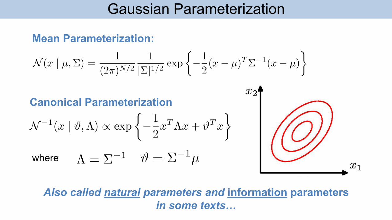
Canonical Parameterization
Gaussian Parameterization
Mean Parameterization:
where
Also called natural parameters and information parameters in some texts…

Gaussian Belief Propagation
Computing marginal mean and covariance from messages:

Gaussian Belief Propagation
Computing marginal mean and covariance from messages:
Compute message mean & covar as algebraic function of incoming message mean & covar (generalizes Kalman)
For tree of N nodes of dimension d, cost is O(Nd3)

LDS Summary
where
Linear dynamical system,
Linear Gaussian Dynamics Linear Gaussian Observation
State-space representation same as linear regression,
Exact posterior inference via Kalman filter• Recursively pass marginal moments• Two steps: prediction, measurement update• Forward pass filtering, backward pass smoothing
Kalman is special case of Gaussian sum-product BP

Outline
• Sequence Models
• Linear Dynamical Systems
• LDS Extensions

Nonlinear Dynamical System
Pendulum with mass m=1,pole length L=1:
Nonlinear dynamics / measurement:

Nonlinear Dynamical System
Filter equations lack a closed-form:Prediction:
Measurement Update:
Idea Linearize f(.) and h(.) about a point m:
where is Jacobian matrix of partials
1st Order Taylorexpansion
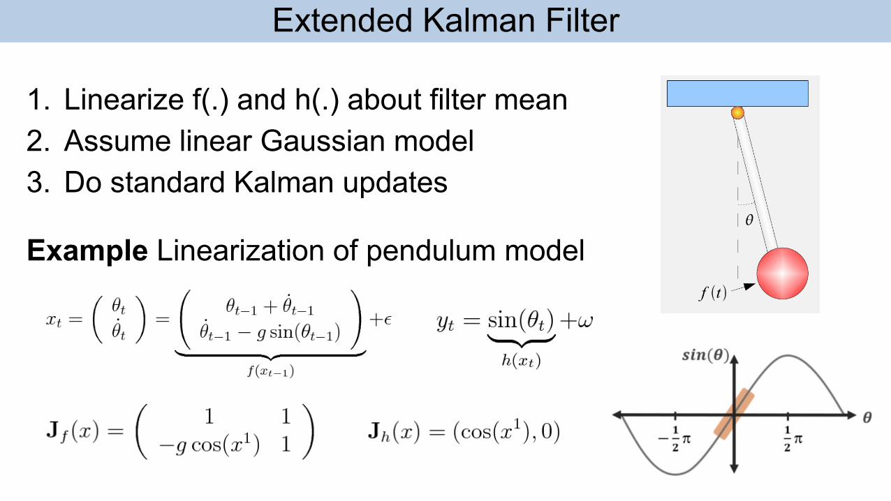
Extended Kalman Filter
1. Linearize f(.) and h(.) about filter mean2. Assume linear Gaussian model3. Do standard Kalman updates
Example Linearization of pendulum model

EKF Update Equations
xt-1 xt…
yt-1
xt-1 xt…
ytyt-1
Measurement Update Step:
Filter Covariance:Filter Mean:
Gain:
Prediction Step:State Prediction:
Covariance Prediction:
Extended Kalman Filter
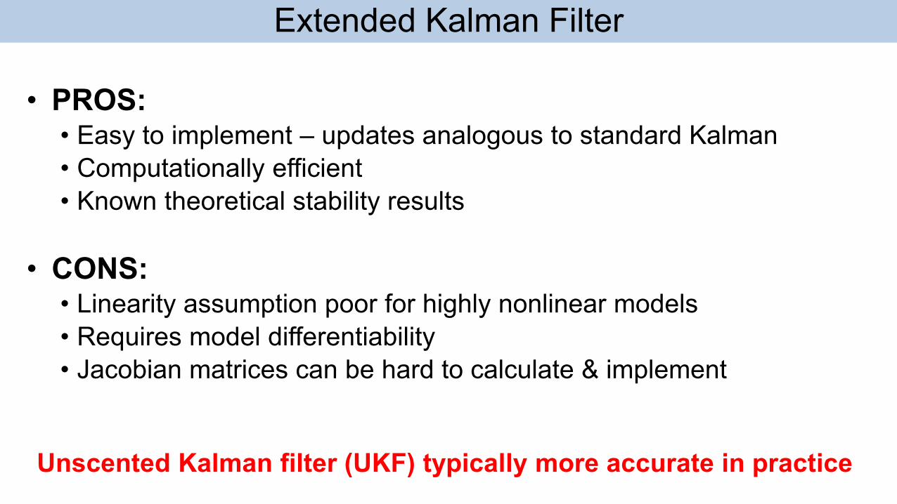
• PROS:• Easy to implement – updates analogous to standard Kalman• Computationally efficient• Known theoretical stability results
• CONS:• Linearity assumption poor for highly nonlinear models• Requires model differentiability• Jacobian matrices can be hard to calculate & implement
Unscented Kalman filter (UKF) typically more accurate in practice

Dynamic Bayesian Networks
• Multivariate latent state (e.g. )• Dynamics for each component within and across time• Sometimes used as catch-all term for dynamical systems
…
t=1 t=2 t=3 t=…
3D latent state x
Caution: DBN terminology is somewhat vague and overloaded (e.g. Deep
Belief Net)

Switching Linear Dynamical System
…
…
Discrete switching state:With stochastic transition matrix
Switching state selects linear dynamics:[ Video: Isard & Blake, ICCV 1998. ]
(e.g. Linear Gaussian )
Colors indicate 3 writing modes
Discrete SwitchingState
ContinuousState

Switching Linear Dynamical System
We can do sum-product for HMM and LDS, so maybe we can do it for SLDS…
…
…
Forward message,
Message is Gaussian mixture over K states (for some K) But incoming message is also a Gaussian mixture Number of components (K) grows exponentially with time t
Integrates to Gaussian foreach possible state zt-1
One way is to use sample-based methods (Particle Filter)

Summary
• Linear dynamical system is time-extension of PCA,
• Exact inference via Kalman filtering,
xt-1 xt…
yt-1
xt-1 xt…
ytyt-1
Prediction step updates moments of predictive distribution
Measurement stepupdates filter distribution with newest measumrent
• Kalman filter is special case of Gaussian belief propagationMessages represented as
Gaussian natural parameters

Summary
• Nonlinear state-space models allow more complex dynamics,
Approximate Kalman filter inference via linearization
(Extended Kalman Filter) or Gaussian quadrature
(Unscented Kalman Filter)
• Switching state-space model represents discrete & continuous states,
…
…Exact inference intractable due to exponential growth in message
parametersBoth nonlinear and SSMs can be
addressed using sample-based methods (e.g. Particle Filtering) as we will see
Related Documents