CS720 Class Notes Steve Revilak Jan 2007 – May 2007

Welcome message from author
This document is posted to help you gain knowledge. Please leave a comment to let me know what you think about it! Share it to your friends and learn new things together.
Transcript

CS720 Class Notes
Steve Revilak
Jan 2007 – May 2007

This are Stephen Revilak’s course notes from CS720, Logical Foundations of Computer Science. Thiscourse was taught by Professor Peter Fejer at UMass Boston, during the Spring 2007 Semester.
Copyright c© 2008 Steve Revilak. Permission is granted to copy, distribute and/or modify this documentunder the terms of the GNU Free Documentation License, Version 1.2 or any later version publishedby the Free Software Foundation; with no Invariant Sections, no Front-Cover Texts, and no Back-CoverTexts. A copy of the license is included in the section entitled “GNU Free Documentation License”.

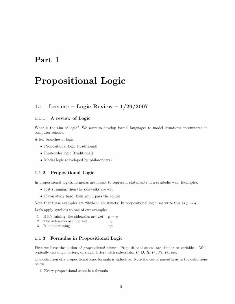
Part 1
Propositional Logic
1.1 Lecture – Logic Review – 1/29/2007
1.1.1 A review of Logic
What is the aim of logic? We want to develop formal languages to model situations encountered incomputer science.
A few branches of logic:
• Propositional logic (traditional)
• First-order logic (traditional)
• Modal logic (developed by philosophers)
1.1.2 Propositional Logic
In propositional logica, formulas are meant to represent statements in a symbolic way. Examples:
• If it’s raining, then the sidewalks are wet
• If you study hard, then you’ll pass the course
Note that these examples are “if-then” constructs. In propositional logic, we write this as p→ q.
Let’s apply symbols to one of our examples
1 If it’s raining, the sidewalks are wet p→ q2 The sidewalks are not wet ¬q3 It is not raining ¬p
1.1.3 Formulas in Propositional Logic
First we have the notion of propositional atoms. Propositional atoms are similar to variables. We’lltypically use single letters, or single letters with subscripts: P , Q, R, P1, P2, P3, etc.
The definition of a propositional logic formula is inductive. Note the use of parenthesis in the definitionsbelow.
1. Every propositional atom is a formula
5

6 CS 720 Class Notes
2. If φ is a formula, then so is (¬φ).
3. If φ and ψ are formulas, then so is (φ ∨ ψ).
4. If φ and ψ are formulas, then so is (φ ∧ ψ).
5. If φ and ψ are formulas, then so is (φ→ ψ).
Suppose we wanted to give a rigorous proof that
((p→ q) ∨ (r ∧ s))
were a valid formula.
Proof
1 p is a formula Rule 12 q is a formula Rule 13 (p→ q) is a formula Rule 5, lines 1, 24 r is a formula Rule 15 s is a forumla Rule 16 (r ∧ s) is a formula Rule 4, Lines 4, 57 ((p→ q) ∨ (r ∧ s)) is a formula Rule 3, lines 3, 6
An example of something that isn’t a formula by the definitions given
(¬p ∨ q)
Informally, we’d treat this as ((¬p) ∨ q), but it doesn’t fit the formal definition.
Precedence in Propositional Logic
The order of precedence is
¬∨, ∧→
Precedence allows us to write
¬p ∨ q → r ∧ s
which is equivalent to the formal
(((¬p) ∨ q)→ (r ∧ s))
1.1.4 Syntax vs. Semantics
Convention: Upper-case greek letters represent sets of formulas, while lower-case greek letters representsingle formulas.
Consider the following two notations
Γ ` φΓ � φ
In each of these cases φ is a single formula and Γ is a set of formula. (Γ may be an empty set).

CS 720 Class Notes 7
• Γ ` φ means that φ can be derived from from formulas in Γ by using some formal proof system.
• Γ � φ means that φ follows logically from Γ. For every situation where Γ holds, φ holds.
• Γ ` φ is a syntactic definition
• Γ � φ is a semantic definition
In many logic systems, we desire the following:
Γ ` φ IFF Γ � φ (1.1.1)
Equation (1.1.1) can be broken into two components:
If Γ ` φ, then Γ � φ This is called soundness (1.1.2)If Γ � φ, then Γ ` φ This is called completeness (1.1.3)
• Soundness is a syntactic quality, and the more important of the two. Soundness means that whenyou prove something, the result really does follow. Soundness allows you to trust the proof system.
• Completeness is a semantic quality. Completeness is useless without soundness.
1.1.5 Natural Deduction
Natural Deduction is a system due to Gentzen. It’s a syntactic system (Γ ` φ).
The following is referred to as a sequent
φ1, φ2, . . . , φn ` ψ (1.1.4)
A sequent is “valid” if one can derive ψ from the premises φ1, φ2, . . . , φn using the rules of naturaldeduction.
The general idea – we will have introduction rules and elimination rules for each connective. Introductionrules allow a connective to be used; elimination rules allow a connective to be removed.
Conjunction (∧)
φ, ψ
φ ∧ ψRule: ∧i (1.1.5)
φ ∧ ψφ
Rule: ∧e1 (1.1.6)
φ ∧ ψψ
Rule: ∧e2 (1.1.7)
In the equations above, the subscript i denotes introduction and the subscript e denotes elimination.
Example 1.1.1: prove the following
P ∧Q, R ` P ∧R
Proof.
1 P ∧Q Premise2 R Premise3 P ∧e1 , Line 14 P ∧R ∧i, Lines 3, 2

8 CS 720 Class Notes
It’s also possible to represent such proofs as a tree.
(Note to self, try installinghttp://www.phil.cam.ac.uk/teaching staff/Smith/LaTeX/nd.html which does the tree representa-tions natively.
Double Negation (¬¬)
¬¬φφ
Rule: ¬¬e (1.1.8)
φ
¬¬φRule: ¬¬i (1.1.9)
Example 1.1.2: Prove
P, (¬¬Q ∧R) ` ¬¬P ∧Q (1.1.10)
Proof:
1 P Premise2 (¬¬Q ∧R) Premise3 ¬¬Q ∧e1 , Line 24 Q ¬¬e, Line 35 ¬¬P ¬¬i, Line 16 ¬¬P ∧Q ∧i, lines 5, 4
Implication
φ, φ→ ψ
ψRule: →e, Modus ponens (1.1.11)
¬ψ, φ→ ψ
¬φRule: Modus Tollens (MT) (1.1.12)
1.1.6 Proof Boxes
When doing proofs, we will use boxes to make temporal assumptions. For example
φ...ψ
φ→ ψRule: →i (1.1.13)
In (1.1.13), we assume that φ is true, and from this assumption derive ψ. The first and last lines of thebox form an implication, φ→ ψ.
Rules for boxes:
• The first line of the box must introduce a temporal assumption. This assumption is not a premise.It is only valid within the box.
• Boxes can be opened at any time (but they must nest properly)
• All boxes must be closed before the last line of the proof.
• In justifying a proof line, one cannot use a previous box that has closed already. (Think of it likethis: assumptions have lexical scope in which they are valid)

CS 720 Class Notes 9
• The line immediately following a closed box has to match the pattern of the conclusion of the rulethat uses the box.
Example 1.1.3:
Outside the box
a line
First line of A
...
Last line of A
First line of B
...
Last Line of B
First line of C
...
Last Line of C
The end
In this example, lines inside C cannot reference lines inside A or B. However, C can reference lines 1and 2.
(For typesetting, we make use of the proofbox package,http://www.cs.man.ac.uk/~pt/proofs/)
Example 1.1.4: Another example, but with a real proof
P → Q ` ¬Q→ ¬P
Proof:
P → Q premise
¬Q assumption
¬P Modus Tollens. 1,2
¬Q→ ¬P →i, 2-3
Example 1.1.5: Another example
` P → P
Proof:
P assumption
P → P →i. 1–1
These kinds of boxed assumptions will often be used to introduce implication.
1.1.7 Theorems
Given the form
Γ ` φ
10 CS 720 Class Notes
where Γ is an empty set, we have the construct
` φ
In this context φ is referred to as a theorem.
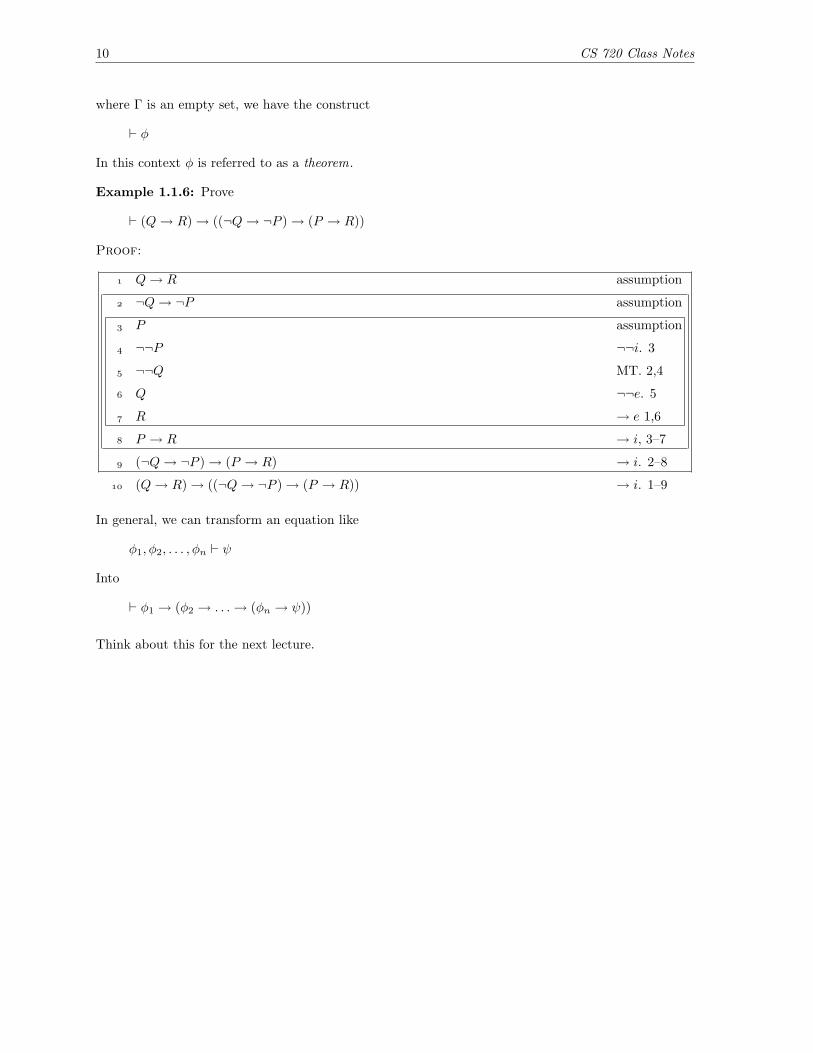
Example 1.1.6: Prove
` (Q→ R)→ ((¬Q→ ¬P )→ (P → R))
Proof:
Q→ R assumption
¬Q→ ¬P assumption
P assumption
¬¬P ¬¬i. 3
¬¬Q MT. 2,4
Q ¬¬e. 5
R → e 1,6
P → R → i, 3–7
(¬Q→ ¬P )→ (P → R) → i. 2–8
(Q→ R)→ ((¬Q→ ¬P )→ (P → R)) → i. 1–9
In general, we can transform an equation like
φ1, φ2, . . . , φn ` ψ
Into
` φ1 → (φ2 → . . .→ (φn → ψ))
Think about this for the next lecture.

CS 720 Class Notes 11
1.2 Lecture – 1/31/2007
1.2.1 Syntax and Semantics
The formula
φ1, . . . , φn ` ψ
is a syntactic representation. Starting with premises φ1, . . . , φn, we apply formal rules to derive ψ. Thisderiviation is done without regard to any assignment of truth values in the formulas.
Assignment of truth values is a semantic representation.
1.2.2 Implications and Assumptions
For proofs that involve implication, a general strategy is as follows:
• Use elimination rules to deconstruct assumptions that have been made.• Use introduction rules to construct the final conclusion.
1.2.3 Disjunction (∨)
For disjunction, we have two introduction rulesφ
φ ∨ ψRule: ∨i1 (1.2.1)
ψ
φ ∨ ψRule: ∨i2 (1.2.2)
Eliminating disjunctions is a little harder. Suppose we have φ ∨ ψ and wish to prove χ. Because wedon’t know which of φ or ψ is true, we have to show both cases. All told, there will be three parts toor-elimination.
• φ ∨ ψ• φ true makes χ true• ψ true makes χ true
The rule for disjunction elimination is
φ ∨ ψφ...χ
ψ...χ
χRule: ∨e (1.2.3)
Example 1.2.1: p ∨ q ` q ∨ p
Proof:
p ∨ q premise
p assumption
q ∨ p ∨i2. 2
q assumption
q ∨ p ∨i1. 4
q ∨ p ∨e. 1, 2–3, 4–5
12 CS 720 Class Notes
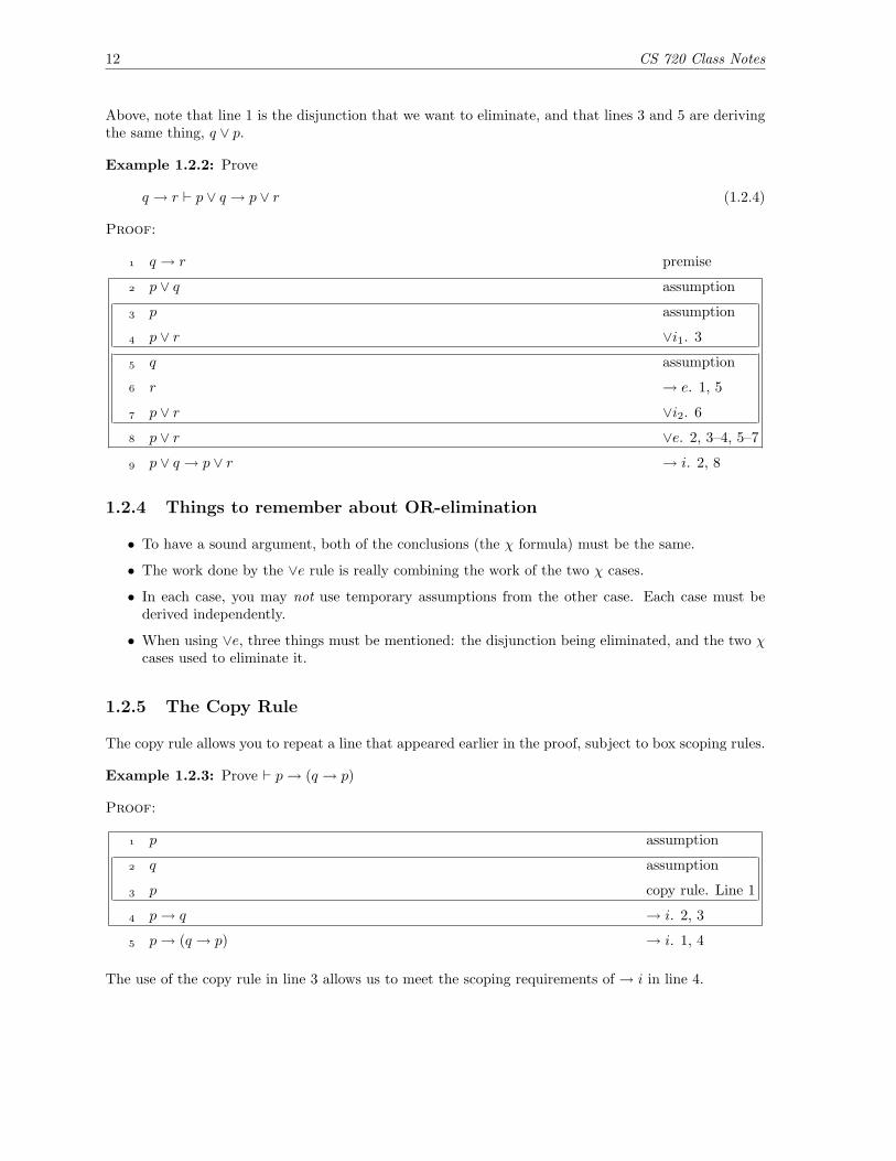
Above, note that line 1 is the disjunction that we want to eliminate, and that lines 3 and 5 are derivingthe same thing, q ∨ p.
Example 1.2.2: Prove
q → r ` p ∨ q → p ∨ r (1.2.4)
Proof:
q → r premise
p ∨ q assumption
p assumption
p ∨ r ∨i1. 3
q assumption
r → e. 1, 5
p ∨ r ∨i2. 6
p ∨ r ∨e. 2, 3–4, 5–7
p ∨ q → p ∨ r → i. 2, 8
1.2.4 Things to remember about OR-elimination
• To have a sound argument, both of the conclusions (the χ formula) must be the same.
• The work done by the ∨e rule is really combining the work of the two χ cases.
• In each case, you may not use temporary assumptions from the other case. Each case must bederived independently.
• When using ∨e, three things must be mentioned: the disjunction being eliminated, and the two χcases used to eliminate it.
1.2.5 The Copy Rule
The copy rule allows you to repeat a line that appeared earlier in the proof, subject to box scoping rules.
Example 1.2.3: Prove ` p→ (q → p)
Proof:
p assumption
q assumption
p copy rule. Line 1
p→ q → i. 2, 3
p→ (q → p) → i. 1, 4
The use of the copy rule in line 3 allows us to meet the scoping requirements of → i in line 4.
CS 720 Class Notes 13
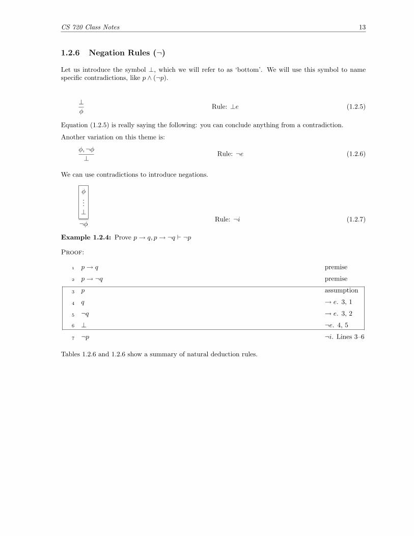
1.2.6 Negation Rules (¬)
Let us introduce the symbol ⊥, which we will refer to as ‘bottom’. We will use this symbol to namespecific contradictions, like p ∧ (¬p).
⊥φ
Rule: ⊥e (1.2.5)
Equation (1.2.5) is really saying the following: you can conclude anything from a contradiction.
Another variation on this theme is:
φ,¬φ⊥
Rule: ¬e (1.2.6)
We can use contradictions to introduce negations.
φ...⊥
¬φRule: ¬i (1.2.7)
Example 1.2.4: Prove p→ q, p→ ¬q ` ¬p
Proof:
p→ q premise
p→ ¬q premise
p assumption
q → e. 3, 1
¬q → e. 3, 2
⊥ ¬e. 4, 5
¬p ¬i. Lines 3–6
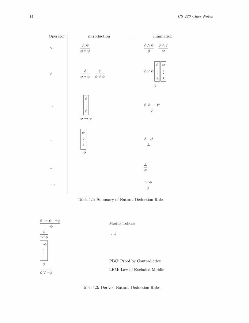
Tables 1.2.6 and 1.2.6 show a summary of natural deduction rules.
14 CS 720 Class Notes
Operator introduction elimination
∧ φ, ψ
φ ∧ ψφ ∧ ψφ
φ ∧ ψψ
∨ φ
φ ∨ ψψ
φ ∨ ψφ ∨ ψ
φ...χ
ψ...χ
χ
→
φ...ψ
φ→ ψ
φ, φ→ ψ
ψ
¬
φ...⊥
¬φ
φ,¬φ⊥
⊥⊥φ
¬¬ ¬¬φφ
Table 1.1: Summary of Natural Deduction Rules
φ→ ψ, ¬ψ¬φ
Modus Tollens
φ
¬¬φ¬¬i
¬φ...⊥
φPBC: Proof by Contradiction
φ ∨ ¬φLEM: Law of Excluded Middle
Table 1.2: Derived Natural Deduction Rules

CS 720 Class Notes 15
Example 1.2.5: Deriving Modus Tollens
φ→ ψ,¬ψ¬φ
(1.2.8)
Proof:
φ→ ψ premise
¬ψ premise
φ assumption
ψ → e. 3, 1
⊥ ¬e. 4, 2
¬φ ¬e. 3–5
Example 1.2.6: Derive
φ
¬¬φ(1.2.9)
Proof:
φ premise
¬φ assumption
⊥ ¬e. 1, 2
¬¬φ ¬i. 2–3
1.2.7 Law of Excluded Middle
Formally, the law of excluded middle (LEM , for short) is stated as follows:
φ ∨ ¬φRule: LEM (1.2.10)
There are no premises. This is also known as an axiom.
In essense, this axiom is saying “either φ is true or it’s not”. (There’s no in-between).
Example 1.2.7: Derivation of the law of excluded middle.
Proof:
¬(φ ∨ ¬φ) assumption
φ assumption
φ ∨ ¬φ ∨i1. Line 2
⊥ ¬e 3, 1
¬φ ¬i. 2–4
φ ∨ ¬φ ∨i2. 5
⊥ ¬e. 6, 1
¬¬(φ ∨ ¬φ) ¬i. 1–7.
φ ∨ ¬φ ¬¬e. 8
16 CS 720 Class Notes
1.2.8 Provable Equivalence
We say that Two formulas, φ and ψ are provably equivalent
φ a` ψ
if φ ` ψ and ψ ` φ.
1.2.9 Intuitionism
Intuitionism is a set of mathematical beliefs. In a nutshell, the intuitionist view requires direct proofs.For example an intuitionist would not accept the notion of φ being true if it were proven by showing ¬φwere a contradiction.
‘Classical’ mathematicians accept proof by contradiction.
Consider the following example.
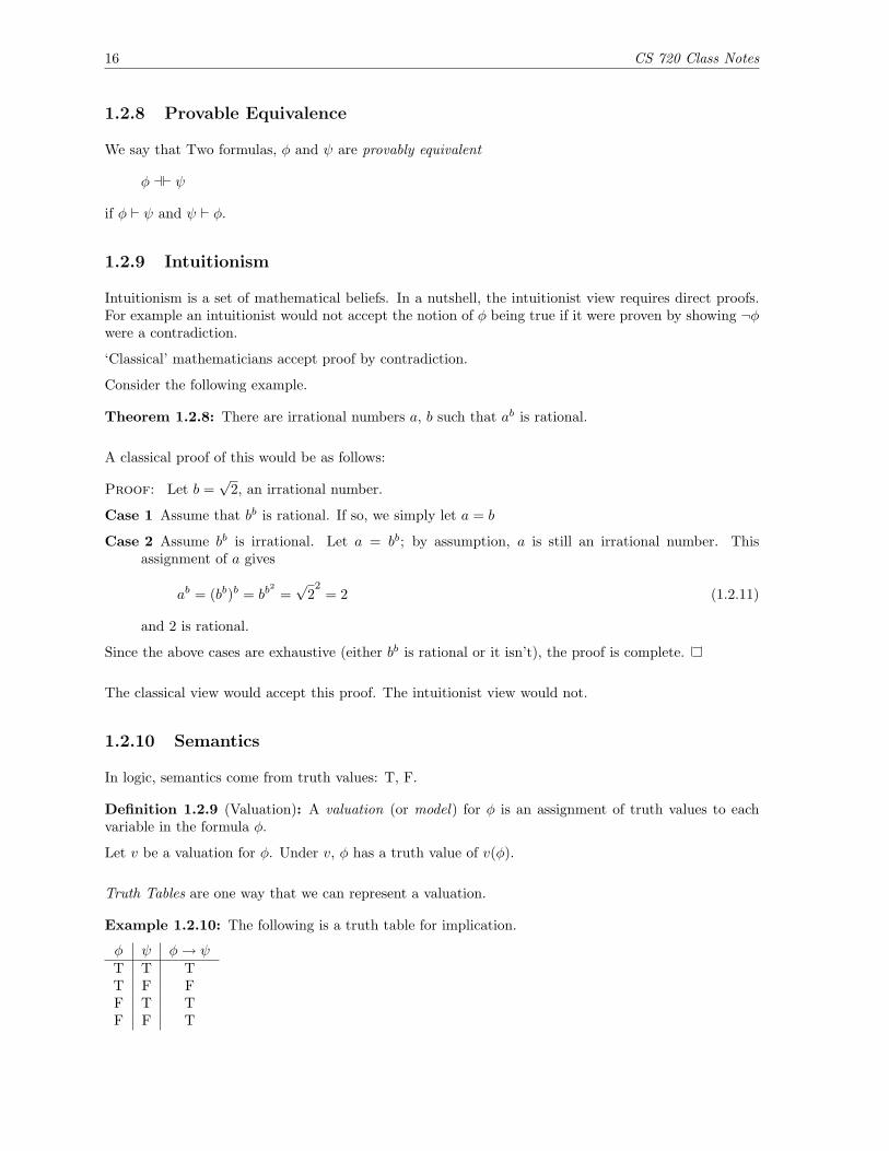
Theorem 1.2.8: There are irrational numbers a, b such that ab is rational.
A classical proof of this would be as follows:
Proof: Let b =√
2, an irrational number.
Case 1 Assume that bb is rational. If so, we simply let a = b
Case 2 Assume bb is irrational. Let a = bb; by assumption, a is still an irrational number. Thisassignment of a gives
ab = (bb)b = bb2
=√
22
= 2 (1.2.11)
and 2 is rational.
Since the above cases are exhaustive (either bb is rational or it isn’t), the proof is complete.
The classical view would accept this proof. The intuitionist view would not.
1.2.10 Semantics
In logic, semantics come from truth values: T, F.
Definition 1.2.9 (Valuation): A valuation (or model) for φ is an assignment of truth values to eachvariable in the formula φ.
Let v be a valuation for φ. Under v, φ has a truth value of v(φ).
Truth Tables are one way that we can represent a valuation.
Example 1.2.10: The following is a truth table for implication.
φ ψ φ→ ψT T TT F FF T TF F T

CS 720 Class Notes 17
Another example of semantic notation:
φ1, . . . , φn � ψ (1.2.12)
Equation (1.2.12) is valid if every valuation to the variables φ1, . . . , φn, ψ that makes φ1 . . . φn true alsomakes ψ true.
Example 1.2.11: p, p→ q � q. This can be verified by looking at the truth table for implication.
Another rule
⊥ � φ for all φ (1.2.13)
We also have tautologies
� φ (1.2.14)
If φ is a tautology, then every truth assignment makes φ true.
1.2.11 Box Rules
The following is a list of rules for using boxes. We’ll use this list when proving soundness and complete-ness.
BOX1 In a proof, all boxes must be closed before the last line of the proof.
BOX2 Boxes must be properly nested.
BOX3a Once a box closes, no line in the box can be referenced later
BOX3b Once a box is closed, no box strictly inside the closed box can be referenced later.
1.2.12 Soundness
Theorem 1.2.12 (Soundness Theorem): If
φ1, . . . , φn ` ψ
then
φ1, . . . , φn � ψ
Put another way, syntax implies semantics.
A proof of this appears in the lecture notes for the next class (page 20).
18 CS 720 Class Notes
1.3 Soundness, Completeness, and CNF (Text Notes)
These are notes from Huth & Ryan, Chapter 1
1.3.1 Soundness And Completeness
` is a syntactic notion.� is a semantic notion. � is also called semantic entailment .
Soundness If φ1, . . . , φn ` ψ holds, then so does φ1, . . . , φn � ψ.
Completeness Wherever φ1, . . . φn � ψ holds, there exists a natural deduction proof of φ1, . . . φn ` ψ
Consider the formula
� φ1 → (φ2 → (φ3 → . . .→ (φn → ψ))) (1.3.1)
Because (1.3.1) is a chain of implications, the formula will hold unless ψ is false.
Theorem 1.3.1 (Soundness and Completeness): Let φ1, . . . , φn, ψ be formulas of propositional logic.Then φ1, . . . , φn � ψ holds IFF the sequent φ1, . . . φn ` ψ is valid.
Soundness means that whatever we prove will be a true fact, based on truth tables.
Completeness means that no matter what (semantically) valid sequents there are, they all have syntacticproofs in the system of natural deduction.
We define equivalence of formulas using �. If φ semantically entails ψ and vice versa, then φ and ψ arethe same as far as our truth table semantics are concerned.
Definition 1.3.2 (Semantic Equivalence): φ and ψ are semantically equivalent if φ � ψ and ψ � φ hold.In this case, we write φ ≡ ψ.
Definition 1.3.3 (Validity): We say that φ is valid if � φ holds.
Example 1.3.4: The following are valid formulas
p→ q ≡ ¬q → ¬pp→ q ≡ ¬p ∨ q
p ∧ q → p ≡ r ∨ ¬r
Definition 1.3.5 (Tautology): η is a tautology if � η holds.
Lemma 1.3.6: Given formulas of propositional logic φ1, . . . , φn, ψ
φ1, . . . , φn � ψ
holds IFF
� φ1 → (φ2 → (φ3 → . . .→ (φn → ψ)))
holds.
Definition 1.3.7 (Conjunctive Normal Form): A formula C is in conjunctive normal form (CNF) if Cis a conjunction of clauses, where each clause D is a disjunction of literals. Example:
(a ∨ b) ∧ (c ∨ d ∨ e) ∧ (f)

CS 720 Class Notes 19
Definition 1.3.8 (Satisfiable): A formula φ in propositional logic is satisfiable if φ has a valuation suchthat v(φ) = T
Satisfiability is a weaker concept than validity. For example,
p ∨ q → p
is satisifiable; the formula will be true whenever p = T. However, p ∨ q → p is not valid – it evaluatesto false when p = F and q = T.
It is possible to specify a forumula φ by its truth table alone. In this case, we don’t know how φ appearssyntactically, but we know how φ is supposed to “behave”.
20 CS 720 Class Notes
1.4 Lecture – 2/5/2007
1.4.1 Soundness
As noted earlier, soundness is a quality whereby
φ1, . . . , φn ` ψ guarantees φ1, . . . , φn � ψ
This is referred to as the soundness theorem
1.4.2 Proof of the Soundness Theorem
Here’s a partial proof, using course-of-values induction.1
Let us define M(k)
M(k) : If φ1, . . . , φn ` ψ by a proof of length k, then φ1, . . . , φn � ψ.
Let us fix k ≥ 1, and assume M(k′) is true for all k′ such that 1 ≤ k′ ≤ k.
Let φ1, . . . , φn ` ψ be a proof of length k.
The following list of cases base the justification on the last line.
1. Premise. If the last line is a premise, then ψ is the same as some φi, and we need to showφ1, . . . , φn � φi.
2. Assumption. The last line of the proof cannot be an assumption, by rule BOX1.
3. Rule ∧e. If the last line of the proof is ∧e, then the last line cannot be part of a box. By theinductive hypothesis, φ1, . . . , φn � φ ∧ ψ, so φ1, . . . , φn � ψ.
4. ⊥. If the last line of the proof is ⊥ from the application of ¬e, then by the inductive hypothesis,we have
φ1, . . . , φn � φ
φ1, . . . , φn � ¬φ
There is no truth assignment that makes φ1, . . . , φn true, so
φ1, . . . , φn � ⊥
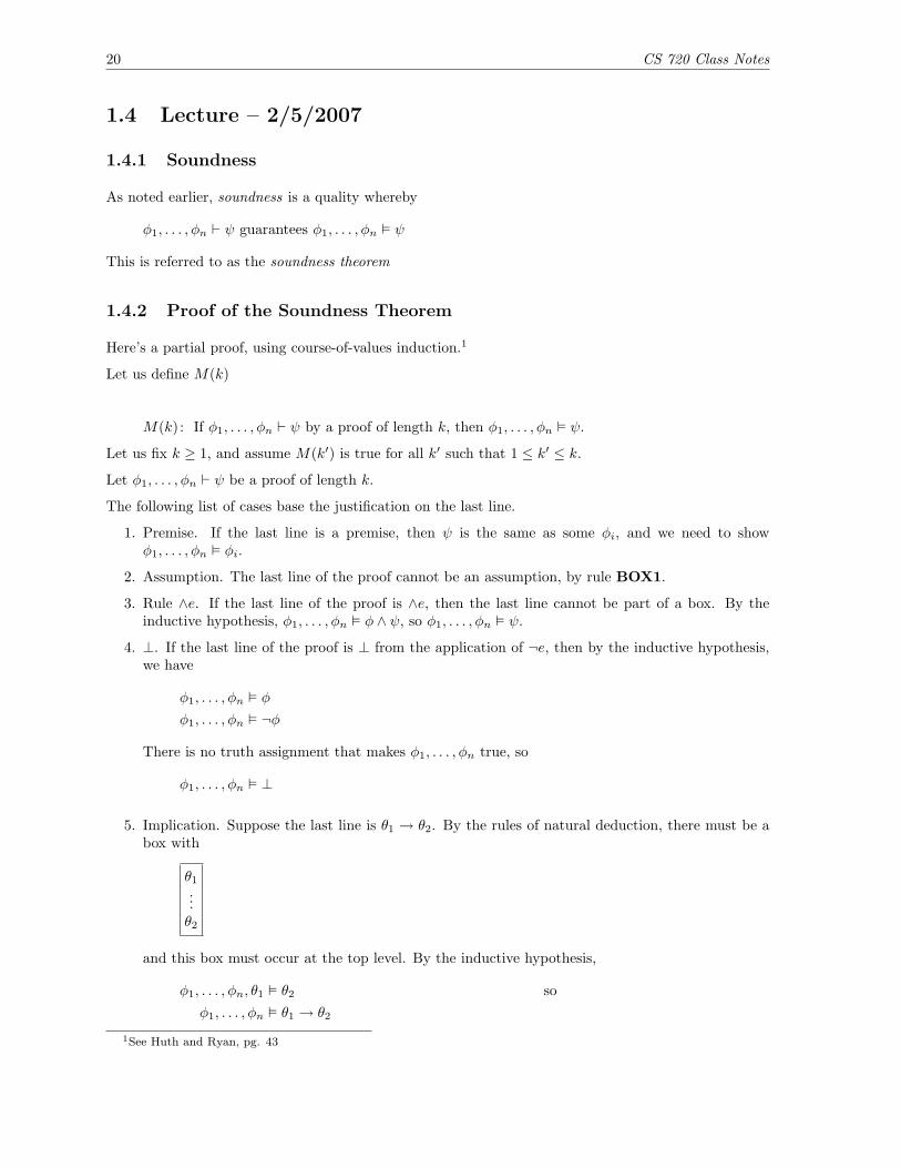
5. Implication. Suppose the last line is θ1 → θ2. By the rules of natural deduction, there must be abox with
θ1...θ2
and this box must occur at the top level. By the inductive hypothesis,
φ1, . . . , φn, θ1 � θ2 soφ1, . . . , φn � θ1 → θ2
1See Huth and Ryan, pg. 43
CS 720 Class Notes 21
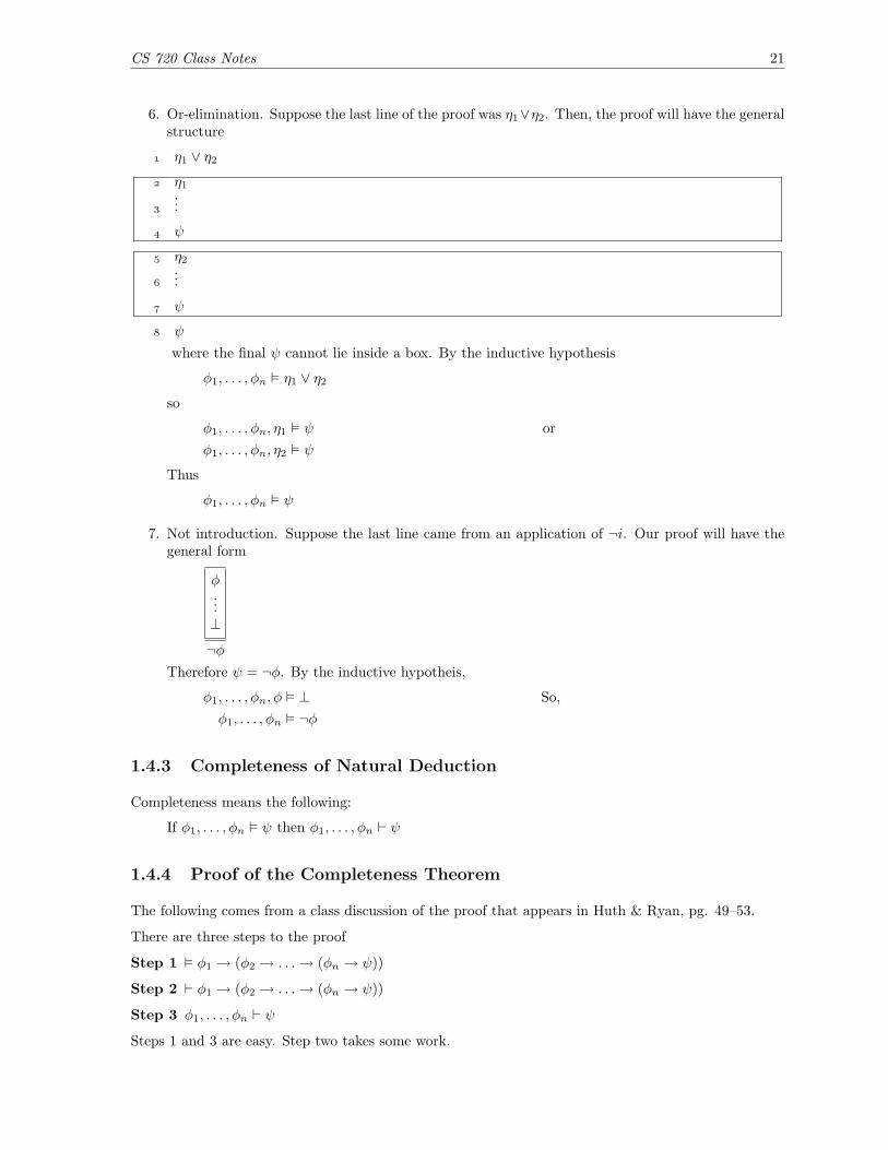
6. Or-elimination. Suppose the last line of the proof was η1∨η2. Then, the proof will have the generalstructure
η1 ∨ η2 η1
...
ψ
η2
...
ψ
ψ
where the final ψ cannot lie inside a box. By the inductive hypothesis
φ1, . . . , φn � η1 ∨ η2so
φ1, . . . , φn, η1 � ψ orφ1, . . . , φn, η2 � ψ
Thus
φ1, . . . , φn � ψ
7. Not introduction. Suppose the last line came from an application of ¬i. Our proof will have thegeneral form
φ...⊥
¬φTherefore ψ = ¬φ. By the inductive hypotheis,
φ1, . . . , φn, φ � ⊥ So,φ1, . . . , φn � ¬φ
1.4.3 Completeness of Natural Deduction
Completeness means the following:
If φ1, . . . , φn � ψ then φ1, . . . , φn ` ψ
1.4.4 Proof of the Completeness Theorem
The following comes from a class discussion of the proof that appears in Huth & Ryan, pg. 49–53.
There are three steps to the proof
Step 1 � φ1 → (φ2 → . . .→ (φn → ψ))
Step 2 ` φ1 → (φ2 → . . .→ (φn → ψ))
Step 3 φ1, . . . , φn ` ψ
Steps 1 and 3 are easy. Step two takes some work.
22 CS 720 Class Notes
Completeness Proof: Step 1
� φ1 → (φ2 → . . .→ (φn → ψ)) (1.4.1)
is expressing a tautology . Because it is a nested implication, (1.4.1) can be false only if ψ = F. However,ψ = F would contradict φ1, . . . , φn � ψ.
Therefore (1.4.1) holds.
Completeness Proof: Step 2
Step 2 is really saying the following
Theorem 1.4.1: If � η holds, then ` η is valid. In other words, if η is a tautology , then η is also atheorem.
Suppose η holds. Then η contains n distinct propositional atoms p1, . . . , pn. Because η is a tautology,each of the 2n lines in η’s truth table evaluates to T. We’ll devise an approach that allows us to take all2n sequents and assemble them into a proof for η.
Lemma 1.4.2: Let φ have propositional atoms p1, . . . , pn. Let L be a line in φ’s truth table. For1 ≤ i ≤ n, let pi = pi if pi = T in line L. Otherwise, let pi = ¬pi. Then, we have
1. p1, . . . , pn ` φ is provable if the entry for φ in line L is T.
2. p1, . . . , pn ` ¬φ is provable if the entry for φ in line L is F.
Lemma 1.4.2 can be proven by induction on φ
Basis. Let φ be some variable p. Then we have one of two cases:
p ` p¬p ` ¬p
Inductive Step 1. Suppose φ = ¬φ1, and assume the result is T for φ1. There are two possibilities:
1. φ = T in line L. Then φ1 = F in line L. By the inductive hypothesis,
p1, . . . , pn ` ¬φ1 = φ
2. Suppose φ = F in line L. Then φi = T in line L. By the inductive hypothesis,
p1, . . . pn ` φ1
p1, . . . pn ` ¬¬φ1 = φ by ¬¬i
Inductive Step 2. Here, φ has the form
φ = φ1 ◦ φ2 for ◦ ∈ {∨,∧,→}
Let q1, . . . , qm be the variables of φ1. Let r1, . . . , rk be the variables of φ2. This gives
{p1, . . . , pn} = {q1, . . . , qm} ∪ {r1, . . . , rk}
CS 720 Class Notes 23
Let L1 be a line in φ1’s truth table corresponding to line L. Let L2 be a line in φ2’s truth tablecorresponding to line L. We have
q1, . . . , qm for line L1
r1, . . . , rk for line L2
Therefore
{p1, . . . , pn} = {q1, . . . , qm} ∪ {r1, . . . , rk}
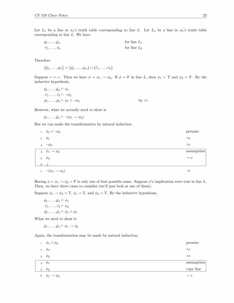
Suppose ◦ =→. Then we have φ = φ1 → φ2. If φ = F in line L, then φ1 = T and φ2 = F. By theinductive hypothesis,
q1, . . . , qm ` φ1
r1, . . . , rk ` ¬φ2
p1, . . . , pn ` φ1 ∧ ¬φ2 by ∧i
However, what we actually need to show is
p1, . . . , pn ` ¬(φ1 → φ2)
But we can make the transformation by natural induction.
φ1 ∧ ¬φ2 premise
φ1 ∧e
¬φ2 ∧e
φ1 → φ2 assumption
φ2 → e
⊥
¬(φ1 → φ2) ¬i
Having φ = φ1 → φ2 = F is only one of four possible cases. Suppose φ’s implication were true in line L.Then, we have three cases to consider (we’ll just look at one of them).
Suppose φ1 → φ2 = T, φ1 = T, and φ2 = T. By the inductive hypothesis,
q1, . . . , qm ` φ1
r1, . . . , rk ` φ2
p1, . . . , pn ` φ1 ∧ φ2
What we need to show is
p1, . . . , pn ` φ1 → φ2
Again, the transformation may be made by natural induction:
φ1 ∧ φ2 premise
φ1 ∧e
φ2 ∧e
φ1 assumption
φ2 copy line
φ1 → φ2 → i
24 CS 720 Class Notes
All told there are 12 cases to consider for φ = φ1 ◦φ2: all four truth table lines for ◦ ∈ {∧,∨,→}. Above,we’ve done two – there are 10 more. Try working a few of them out.
This completes the proof of Lemma 1.4.2. We’ll finish step 2 next.
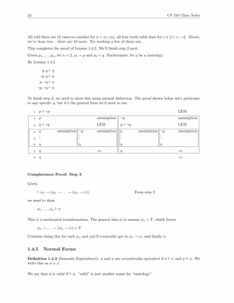
Given p1, . . . , pn, let n = 2, p1 = p and p2 = q. Furthermore, let η be a tautology.
By Lemma 1.4.2
p, q ` η¬p, q ` ηp,¬q ` η¬p,¬q ` η
To finish step 2, we need to show this using natural deduction. The proof shown below isn’t particularto any specific η, but it’s the general form we’d need to use.
p ∨ ¬p LEM
p assumption
q ∨ ¬q LEM
q assumption
...
η
¬q assumption...
η
η ∨e
¬p assumption
q ∨ ¬q LEM
q assumption...
η
¬q assumption...
η
η ∨e
η ∨e
Completeness Proof: Step 3
Given
` φ1 → (φ2 → . . .→ (φn → ψ)) From step 2
we need to show
φ1, . . . , φn ` ψ
This is a mechanical transformation. The general idea is to assume φ1 = T, which forces
φ2 → . . .→ (φn → ψ) = T
Continue doing this for each φi, and you’ll eventually get to φn → ψ, and finally ψ.
1.4.5 Normal Forms
Definition 1.4.3 (Semantic Equivalence): φ and ψ are semantically equivalent if φ � ψ and ψ � φ. Wewrite this as φ ≡ ψ.
We say that φ is valid if � φ. “valid” is just another name for “tautology”.
CS 720 Class Notes 25
Lemma 1.4.4: Given forumulas φ1, . . . , φn, ψ,
φ1, . . . , φn � ψ IFF � φ1 → (φ2 → . . .→ (φn → ψ))
We’ve covered the forward case of this already – we’ll cover the reverse here.
Suppose
φ1 → (φ2 → . . .→ (φn → ψ))
is valid. If a truth assignment makes φ1, . . . , φn true, then it also makes
φ1 → (φ2 → . . .→ (φn → ψ))
true, and it will make ψ true as well. If φ1, . . . , φn were true and ψ = F, this would contradict φ1, . . . , φn �ψ.
This reduces entailment to a tautology.
Truth tables can be used to test validity. However, there’s a disadvantage to this: given n propositionalvariables, the truth table will have 2n rows. In the next lecture, we’ll look at other ways of testingvalidity.

26 CS 720 Class Notes
1.5 Lecture – 2/7/2007
1.5.1 Conjunctive Normal Form (CNF)
A formula φ is in CNF if φ is a conjunction of disjunctions of literals. We can define CNF as a grammar
Literal = p | ¬pDisjunction = Literal | Literal ∨ Disjunction
CNF = Disjunction | Disjunction ∧ CNF
Example 1.5.1: Formulas in CNF
(p ∨ q) ∧ (¬p ∨ ¬q)p ∧ q ∧ r
As the second line shows, it’s okay for a Disjunction to consist of a single Literal.
If a formula φ is in CNF, then there is an easy way to check its validity.
� φ1 ∧ . . . ∧ φn IFF � φ1 and . . . and � φn
φ1 ∧ . . . ∧ φn is valid IFF every φi is valid.
We can state this more formally:
Theorem 1.5.2: A disjunction of literals p1, . . . , pn is valid IFF for some j, k, 1 ≤ j, k ≤ n, pj = ¬pk.
Proof: If j, k exist, then the disjunction is valid (Law of Excluded Middle). However, if no such j, kexist, we can assign a value of F to each pi and make p1 ∨ . . . ∨ pn false.
Truth tables can be used to test validity. Another way to test validity is to construct a proof by naturaldeduction (prove ` φ). A third way to test validity is to convert an arbitrary formula into an equivalentCNF formula, and test the CNF formula.
Definition 1.5.3 (Satisfiable): φ is satisfiable if there is some truth assignment that makes φ true.
validity → satisfiablesatisfiable 9 validity
Note that φ is satisifiable IFF ¬φ is not valid. Therefore, if we can determine validity, then we candetermine satisifiability.
Similarly, φ is valid IFF ¬φ is not satisifiable.
CNF and Computability
Suppose we had a function CNF(φ) that took an arbitrary formula φ and converted it to CNF. CNFoperates under the following conditions:
• CNF(φ) ≡ φ• CNF(φ) is in CNF.
With such a function, we can test if φ is valid by testing whether CNF(φ) is valid.
CNF(φ) could not run in polynomial time. There are formulas φ such that any equivalent formula inconjunctive normal form is exponentially larger. For example:
(X1 ∧ Y1) ∨ (X2 ∧ Y2) ∨ . . . ∨ (Xn ∧ Yn) (1.5.1)

CS 720 Class Notes 27
Equation (1.5.1) is in disjunctive normal form. Converting it to CNF would require many applicationsof distributive laws, resulting in a much longer formula.
1.5.2 Truth Tables and Conjunctive Normal Form
Given a truth table for φ, it is easy to give an equivalent formula in conjunctive normal form. This canbe done even if you don’t know the syntactic structure of φ.
Consider the following truth table
p q r φT T T TT T F TT F T TT F F FF T T TF T F FF F T TF F F F
We turn this into CNF as follows:
1. Take all the lines where φ = F
2. Form a disjunction of variables pi, corresponding to variables in the truth table: pi = ¬pi3. Combine the disjunctions with conjunctions.
In our example, lines 4, 6, 8 are those where φ = F. Our three disjunctions are
¬p ∨ q ∨ r from line 4p ∨ ¬q ∨ r from line 6p ∨ q ∨ r from line 8
Combining these with ∧ gives
(¬p ∨ q ∨ r) ∧ (p ∨ ¬q ∨ r) ∧ (p ∨ q ∨ r)
There is a special case. If all truth table entries are true, then (p ∨ ¬p) is a perfectly good equivalentCNF.
Of course, because one can test validity directly from a truth table, there’s not much sense in going fromtruth table to CNF to validity test.
1.5.3 Procedure for CNF Transformation
The general procedure for turning an arbitrary formula into CNF is as follows:
1. Remove implication, by transforming p→ q to ¬p ∨ q.
2. Push negation inward, using DeMorgan’s laws. We want negation to apply to atoms, not clauses
3. Use distributivity to transform the formula into CNF.
28 CS 720 Class Notes
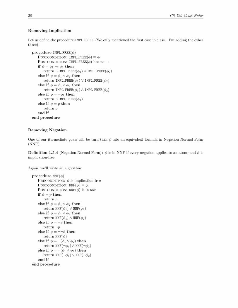
Removing Implication
Let us define the procedure IMPL FREE. (We only mentioned the first case in class – I’m adding the otherthree).
procedure IMPL FREE(φ)Postcondition: IMPL FREE(φ) ≡ φPostcondition: IMPL FREE(φ) has no →if φ = φ1 → φ2 then
return ¬IMPL FREE(φ1) ∨ IMPL FREE(φ2)else if φ = φ1 ∨ φ2 then
return IMPL FREE(φ1) ∨ IMPL FREE(φ2)else if φ = φ1 ∧ φ2 then
return IMPL FREE(φ1) ∧ IMPL FREE(φ2)else if φ = ¬φ1 then
return ¬IMPL FREE(φ1)else if φ = p then
return pend if
end procedure
Removing Negation
One of our itermediate goals will be turn turn φ into an equivalent formula in Negation Normal Form(NNF).
Definition 1.5.4 (Negation Normal Form): φ is in NNF if every negation applies to an atom, and φ isimplication-free.
Again, we’ll write an algorithm:
procedure NNF(φ)Precondition: φ is implication-freePostcondition: NNF(φ) ≡ φPostcondition: NNF(φ) is in NNFif φ = p then
return pelse if φ = φ1 ∨ φ2 then
return NNF(φ1) ∨ NNF(φ2)else if φ = φ1 ∧ φ2 then
return NNF(φ1) ∧ NNF(φ2)else if φ = ¬p then
return ¬pelse if φ = ¬¬φ then
return NNF(φ)else if φ = ¬(φ1 ∨ φ2) then
return NNF(¬φ1) ∧ NNF(¬φ2)else if φ = ¬(φ1 ∧ φ2) then
return NNF(¬φ1) ∨ NNF(¬φ2)end if
end procedure

CS 720 Class Notes 29
Distributing Subformulas
The procedure DISTR implements the distributive laws needed for CNF conversion.
procedure DISTR(η1, η2)Precondition: η1 and η2 are in CNFPostcondition: DISTR(η1, η2) is in CNFPostcondition: DISTR(η1, η2) ≡ η1 ∨ η2if η1 = η11 ∧ η12 then
return DISTR(η11 , η2) ∧ DISTR(η12 , η2)else if η2 = η21 ∧ η22 then
return DISTR(η1, η21) ∧ DISTR(η1, η22)else
return η1 ∨ η2end if
end procedure
The CNF Procedure
Using IMPL FREE, DISTR, and NNF as building blocks, we can now define a procedure CNF that takes anarbitrary formula φ as input and returns an equivalent formula in conjunctive normal form.2
procedure CNF(φ)Precondition: φ is in NNFPostcondition: CNF(φ) ≡ φPostcondition: CNF(φ) is in CNFif φ = p then
return pelse if φ = ¬p then
return ¬pelse if φ = φ1 ∧ φ2 then
return CNF(φ1) ∧ CNF(φ2)else if φ = φ1 ∨ φ2 then
return DISTR(CNF(φ1), CNF(φ2))end if
end procedure
CNF carries the precondition that φ is in NNF. We do the actual CNF conversion with the following call
CNF(NNF(IMPL FREE(φ))) (1.5.2)
In the worst case (1.5.2) will take exponential time. However, there are some inputs where the runningtime will be polynomial.
By contrast, using truth tables always takes exponential time.
1.5.4 Satisfiability Problems
The satisifiability problem is as follows: given a propositional logic formula φ, is φ satisfiable? We’llrefer to this as the SAT Problem
The SAT problem is NP-complete. If we were to find a polynomial-time algorithm for SAT, that wouldimply P = NP. Therefore, it is unlikely that we will find a polynomial time algorithm.
2In our lecture, we called this formula CNF’. I’m using CNF to be consistent with the text

30 CS 720 Class Notes
Earlier, we related satisifiability to validity. φ is not satisifiable if ¬φ is valid, and φ is valid if ¬φ is notsatisifiable. This means that validity cannot be done in polynomial time. (If we had a way to computevalidity in polynomial time, then we’d have a way to compute SAT in polynomial time).
Let’s consider another function: CNF∗(φ), whose properties are as follows:
• CNF∗(φ) is in conjunctive normal form
• φ is valid IFF CNF∗(φ) is valid.
• CNF∗(φ) is computable in polynomial time
Where φ is any formula of propositional logic.
Is such a CNF∗ likely? No, because it would give us a polynomial time test for validity.
Let’s consider another function: CNF∗∗(φ):
• CNF∗∗(φ) is in conjunctive normal form
• φ is valid IFF CNF∗∗(φ) is satisfiable.
• CNF∗∗(φ) is computable in polynomial time
In this case, CNF∗∗(φ) is possible to compute in polynomial time (Why?).
Another example: CNF-SAT(φ). Given a formula in CNF, is φ satisfiable? This is still NP-complete.
In summary
• Validity is easy to check when φ is in CNF• Satisifiability is not easy to check when φ is in CNF
1.5.5 Horn Clauses
Horn clauses are named after Alfred Horn.
Let’s review some notation
⊥ bottom – a contradiction> top – a tautology
> is equivalent to (p ∨ ¬p).
The structure of horn clauses is shown in the following grammar:
P = > | ⊥ | pA = P | P ∧ AC = A → PH = C | C ∧ H
Example 1.5.5: Horn Clauses.
(p1 ∧ p2 ∧ p3 → p4) ∧ (p3 → p5)p1 ∧ p2 → ⊥(> → p2) ∧ (p3 → ⊥)> ∧⊥ ∧> → ⊥
CS 720 Class Notes 31
Horn clauses are equivalent to CNF. For example
p1 ∧ p2 ∧ p3 → p4
=¬(p1 ∧ p2 ∧ p3) ∨ p4
=¬p1 ∨ ¬p2 ∨ ¬p3 ∨ p4
This is just a straightforward application of implication elimination and the DeMorgan laws.
When converted to CNF, there will be one atom which is not negated.
Translation of Horn Clauses to Disjunctions
Suppose we are given the formula
φ = p1 ∧ p2 ∧ . . . ∧ pk → p′
There are a few cases to consider
Case 1 If at least one of pi is ⊥, then φ is a tautology. (pi ∨ ¬pi) is a perfectly good equivalent (forany pi).
Case 2 No pi is ⊥, p′ is an atom. We translate this as
¬pi1 ∨ . . . ∨ ¬pir ∨ p′
¬pi1 ∨ . . . ∨ ¬pir are the atoms in p1 . . . pk. In other words, we leave out >. Example
> ∧ p1 ∧ p2 → p′ ⇒ ¬p1 ∨ ¬p2 ∨ p3
Case 3 No pi is bottom, at least one pi is an atom, and p′ = ⊥. We translate this as
¬pi1 ∨ . . . ∨ ¬pir
Case 4 All pi are >, p′ = ⊥. Example:
> ∧> ∧> → ⊥
This is translated as � (“Box”). Box is an empty disjunction, and it is always false.
Case 5 p′ = >. Here, we have a tautology. We can translate it as (pi ∨ ¬pi) for any pi.
32 CS 720 Class Notes
1.6 Lecture – 2/12/2007
1.6.1 Horn Formulas
To review, horn formulas are defined with the following grammar
P = ⊥ | > | pA = P | P ∧AC = A→ P
H = C | C ∧H
Horn formulas are really just a special case of CNF, where each disjunction has at most one positiveliteral.
Example 1.6.1: Examples of horn formulas
p1 ∧ p2 ∧ > → p3
≡¬p1 ∨ ¬p2 ∨ p3
> ∧> ∧> → ⊥≡� An unsatisifiable formula
We call the symbol � “Box”. Box is an empty disjunction that is not satisifiable. It’s equivalent to(p ∧ ¬p), but has some technical conveniences.
Satisifiablity for CNF formulas is an NP-Complete problem.Validity for CNF forumulas is a P problem (there is an efficient solution).Horn formulas have an efficient algorithm for satisfiability.
1.6.2 Algorithm For Horn Satisfiability
Below is a linear-time algorithm that determines the satisifiability of horn clauses:
procedure HORN(φ)Precondition: φ is a horn formulaPostcondition: HORN returns ‘satisifiable’ if φ is satisfiable; HORN returns unsatisfiable otherwise.Mark >while there is a clause p1 ∧ . . . ∧ pk → p′ such that p1 ∧ . . . ∧ pk are marked but p′ is not marked
doMark p′
end whileif ⊥ is marked then
return “unsatisifiable”else
return “satisfiable”end if
end procedure
Why is this correct?
Claim 1.6.2: If v satisifies φ and p is marked, then v(p) = T.
Proof (Horn Algorithm): Our proof is by induction on the number of iterations of the while loop.
CS 720 Class Notes 33
M(k): if p is marked after k iterations of the while loop, then v(p) = T for any v withv(φ) = T
Basis: k = 0. If p is unmarked before the while loop is entered, then p = >, and v(>) = T.
Inductive Case: Suppose M(k) is true and p is marked the the k + 1 iteration of the while loop. If p ismarked, then there is a clause p1 ∧ . . . ∧ pk → p where p1, . . . .pk are marked after k iterations. By theinductive hypothesis, v(p1), . . . , v(pl) = T. Therefore v(p1 ∧ . . . ∧ pk → p) is true and v(p) is true.
We can also guarantee that the algorithm will terminate on correct input. Each time the loop executes,a new p′ is marked. There are only a finite number of literals to mark, therefore the algorithm mustterminate eventually.
If the output is “unsatisifiable”, then ⊥ is marked. Therefore, any satisfying assignment must make⊥ = T. This is not possible, so there is no satisfying assignment for φ.
If the output is “satisfiable”, then we must define v by v(p) = T if p is a marked atom and v(p) = F ifp is an unmarked atom.
To show that v satisifies φ, it is enough to how that v satisifies each clause p1 ∧ . . . ∧ pk → p′
If any v(pi) = F, then the clause is satisfied.
If v(pi) = T for all i, then each pi is either > or a marked atom. Therefore p′ 6= ⊥; p′ is either (1) > or(2) a marked atom, so v(p′) = T and v(p1 ∧ . . . ∧ pk → p′) = T.
1.6.3 SAT Solvers
Next, we’ll look at an algorithm which takes a formula φ and tries to determine whether φ is satisfiable.
Satisifiability is an NP-complete problem. If we have a P-time algorithm, this algorithm must (1)occassionally give an incorrect answer or (2) be unable to handle some of the problems that is is presentedwith.
We’ll look at two variations of such an algorithm.
For our SAT solver, we will assume that the connectives ¬ and ∧ are adequate. All formulas will betransformed to use these connectives. We define the transformation T (φ) below.
T (p) = p
T (¬φ) = ¬T (φ)T (φ ∧ ψ) = T (φ) ∧ T (ψ)T (φ ∨ ψ) = ¬(¬T (φ) ∧ ¬T (ψ))T (φ→ ψ) = ¬(T (φ) ∧ ¬T (ψ))
Our SAT solver will take a formula using ¬ and ∧ and transform the formula into a DAG. The DAGwill be similar to a parse tree, but each literal will appear only once.
Let’s look at an example
φ = p ∧ ¬(q ∨ ¬p)T (φ) = p ∧ ¬¬(¬q ∧ ¬¬p)
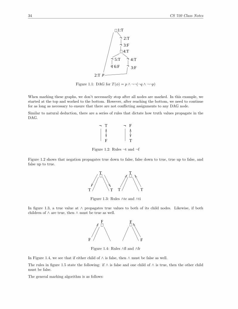
Our first step was to transform φ into T (φ), which uses the desired set of connectives. In figure 1.1, thenumbers denote the order in which nodes were visitied. T and F denote values that a node must havein order to be true. Of course, the root must be marked true.
34 CS 720 Class Notes
2:T
∧
¬
¬
∧
¬¬
¬q
p
1:T
2:T
3:F
4:T
3:F
4:T5:T
6:F
Figure 1.1: DAG for T (φ) = p ∧ ¬¬(¬q ∧ ¬¬p)
When marking these graphs, we don’t necessarily stop after all nodes are marked. In this example, westarted at the top and worked to the bottom. However, after reaching the bottom, we need to continuefor as long as necessary to ensure that there are not conflicting assignments to any DAG node.
Similar to natural deduction, there are a series of rules that dictate how truth values propagate in theDAG.
T
¬ T
F
¬ F
Figure 1.2: Rules ¬t and ¬f
Figure 1.2 shows that negation propagates true down to false, false down to true, true up to false, andfalse up to true.
T∧
TT
T∧
T T
Figure 1.3: Rules ∧te and ∧ti
In figure 1.3, a true value at ∧ propagates true values to both of its child nodes. Likewise, if bothchildren of ∧ are true, then ∧ must be true as well.
FF
∧F
∧F
Figure 1.4: Rules ∧fl and ∧fr
In Figure 1.4, we see that if either child of ∧ is false, then ∧ must be false as well.
The rules in figure 1.5 state the following: if ∧ is false and one child of ∧ is true, then the other childmust be false.
The general marking algorithm is as follows:

CS 720 Class Notes 35
T
∧∧F F
FT F
Figure 1.5: Rules ∧fll and ∧frr
• Mark the root node as T.
• Using rules, push values through the DAG, until no new values can be assigned.
The algorithm will end in one of three states:
1. Not all nodes are marked. In this case, we don’t know whether T (φ) is satisifiable.
2. All notes are marked, and each node is marked with a single truth value. Here, T (φ) is satisfiable,and we have a satisfying assignment.
3. Some nodes are marked both T and F. Here, we know that T (φ) is not satisfiable.
If T (φ) has two or more satisfying assignments, then this algorithm is not sufficient to determine satis-fiability. It will only work for formulas where there is a single satisfying assignment.
Consider the DAG in figure 1.6. Here, we have a formula of the form ¬(φ1 ∧ φ2). We can assign a truthvalue to the root, and push a value one level below. However, after step 2 we’re stuck; there are multiple
¬
∧ 2:F
1:T
Figure 1.6: ¬(φ1 ∧ φ2). We don’t know
satisifying assignments for the children of ∧ that will make ∧ false.
Improvements to the SAT Solver
We can make some improvements to our P-time SAT solver. It still won’t be perfect, but these improve-ments will allow it to find answers for a larger number of cases.
• After the first pass, if some nodes are unmarked, pick an unmarked test node n. Temporarily markn = T and push values around. Next, temporarily mark n = F and push values around. If the twotest values for n lead to contradictions, then declare the formula to be unsatisfiable.
• If both tests lead to application of the same mark to some previously unmarked node m, then wemay mark m permanently.
• If one test value produces a contradiction and the other test value does not, then we can retainthe test value that did not produce a contradition.
• If one test leaves every node marked but does not produce a contradiction, then we can declarethe formula satisfiable and we have a satisfying assignment.
Again, these improvements will NOT yield a perfect algorithm. Satisfiability is an NP-complete problem,so we cannot hope to solve it with a polynomial time algorithm.

36 CS 720 Class Notes
A related lesson: sometimes we are faced with the need to solve an NP-Complete problem. Sometimes,it’s useful to approximate a best answer, if ‘close enough’ is sufficiently good.

Part 2
Predicate Logic
2.1 Lecture – 2/12/2007
Predicate logic is also known as first-order logic.
Predicate logic evolved from the need to express things that propositional logic could not express.Consider the following:
All men are mortal (All A’s are B’s)Socrates is a man (s is an A)Socrates is a mortal (s is a B)
Propositional logic cannot decompose these statements.
Some building blocks for predicate logic
Predicates Predicates take one or more arguments and return a truth value. (Single argument predi-cates are called unary predicates, two-argument predicates are called binary predicates, etc).
Predicates represent properties of individuals
Constants A constant stands for a single individual.
Constants can also be thought of as nullary functions – functions that take no arguments, andalways return a specific value.
Functions Functions take zero or more arguments, and return some single value.
Example 2.1.1: Unary predicates
The moon is green G(m)The wall is green G(w)π is irrational I(π)
Example 2.1.2: Binary predicates
John and Peter are brothers B(j, p)
Example 2.1.3: Functions
John’s father f(j)John’s father is an engineer E(f(j))
37
38 CS 720 Class Notes
2.2 Lecture – 2/21/2007
2.2.1 Predicate Logic
The ingredients of predicate logic are
• Predicate symbols (arity > 0)
• Functions (arity ≥ 0). Functions whose arity is zero are constants.
• Quantifiers – ∀, ∃.
• Variables
Example 2.2.1: John’s father and George are brothers.
B(f(j), g)
Example 2.2.2: Every cow is brown. In propositional logic, we express this as
∀x(Cow(x)→ Brown(x))
Example 2.2.3: Some cows are brown.
∃x(Cow(x) ∧ Brown(x))
This is not the same thing as ∃x(Cow(x) → Brown(x)). With implication, the literal translation is“either x is not a cow or x is brown”. (x could be a brown horse).
Example 2.2.4: Some birds don’t fly.
∃x(Bird(x) ∧ ¬Fly(x))
Example 2.2.5: Not every bird flies.
¬(∀x(Bird(x)→ Fly(x)))
We can manipulate this formula a little
¬(∀x(¬Bird(x) ∨ Fly(x)))¬(∀x¬(Bird(x) ∧ ¬Fly(x)))∃x(Bird(x) ∧ ¬Fly(x))
This example illustrates the relationship between ∀ and ∃.
Relationship between ∀ and ∃
∃xP(x) = ¬∀x¬P(x) (2.2.1)∀xP(x) = ¬∃x¬P(x) (2.2.2)
2.2.2 Components of First Order Logic
Terms. Terms denote objects. Constants, variable, and functions are all examples of terms.
Formulas. Formulas denote truth values – they represent T or F, but not an individual thing.
CS 720 Class Notes 39
Predicate Vocabulary = First order language. Our predicate vocabulary is
• A set P of predicate symbols, each having arity > 0.
• A set F of function symbols, each having arity ≥ 0. The set F includes constants.
We denote this vocabulary by (F ,P).
Terms in (F ,P):
• If x is a variable, then x is a term.
• If a is a nullary function, then a is a term.
• If f is an n-ary function and t1, . . . , tn are terms, then f(t1, . . . , tn) is also a term.
As a BNF, terms are
t ::= x | a | f(t1, . . . , tn) (2.2.3)
Formulas in (F ,P):
• If P is a predicate symbol of arity > 0, and t1, . . . , tn are terms, then P (t1, . . . , tn) is a formula.
• If φ is a formula, then ¬φ is a formula.
• If φ, ψ are formulas, then φ ∧ ψ, φ ∨ ψ, and φ→ ψ are also formulas.
• If φ is a formula and x is a variable, then ∀xφ and ∃xφ are formulas.
• If t1, t2 are terms, then t1 = t2 is a formula (= acts like a binary predicate).
As a BNF, formulas are:
φ ::= P (t1, . . . , tn) | ¬φ | φ ∧ ψ | φ ∨ ψ | φ→ ψ | ∀xφ | ∃xψ | t1 = t2 (2.2.4)
The binding rules for first order logic:
¬,∀x, ∃x∨,∧→ right associative
By right-associative, we mean that q → r → s is interpreted as q → (r → s), not (q → r)→ s.
2.2.3 Bound Quantifiers and Free Quantifiers
Consider the formula
∃x(P (x) ∧ ¬Q(x)) ∨R(y)
x is a bound variable, and y is a free variable. By analogy, inn∑i=1
i2
i is bound, and n is free.
The scope of a quantifier in a formula is the subformula immediately following the quantifier.
An occurrence of a variable x is bound if (1) it immediately follows a quantifier symbol, or (2) it is inthe scope of a quantifer of the same variable. For example, in ∀xP (x), there are two bound occurrencesof x – (1) in ∀x and (2) in P (x).
If an occurrence of a variable is not bound, then it is said to be free.
40 CS 720 Class Notes
Example 2.2.6: Consider the formula.
∀x(P (x, y) ∨R(x)) ∧ ∃zQ(x, y, z)
Here
P (x, y) x is bound, y is freeR(x) x is boundQ(x, y, z) x, y are free; z is bound
Example 2.2.7: Condsider
∃z(P (z) ∧ ∀zR(z))
Here, there are two different bindings for z. In P (z), z is bound to ∃z. In R(z), z is bound to ∀z. Thefollowing two formulas are equivalent:
∃z(P (z) ∧ ∀yR(y))∃w(P (w) ∧ ∀zR(z))
With respect to binding, only the innermost quantifier matters.
2.2.4 Substitution in First-Order Logic
We notate substitution as
φ[t/x] (2.2.5)
This means “take φ, and replace all free occurrences of x with t”.
Example 2.2.8: Substitution.
((∃x(R(x, y)) ∧ (∀zP (x, z))) [f(y)/x]=(∃x(R(x, y)) ∧ (∀zP (f(y), z))
Note that the bound occurrence of x was not replaced, but the unbound occurrence of x was.
Let’s try to come up with an inductive definition for substitution:
R(t1, . . . , tn)[t/x] = R(t1[t/x], . . . , tn[t/x])(¬φ)[t/x] = ¬φ[t/x]
(φ ◦ ψ)[t/x] = φ[t/x] ◦ ψ[t/x] ◦ ∈ {∨,∧,→}
(Qyφ)[t/x] =
{Qyφ if x = y (no change)Qy(φ[t/x]) otherwise
where Q ∈ {∀,∃}
The general idea behind substitution is as follows: when we substitute t for x, φ must say the samething about t that it said about x.
Example 2.2.9: Some (correct) examples of substitution.
∃x(y = 2x) y is even(∃x(y = 2x))[3z/y] = ∃x(3z = 2x) 3z is even
CS 720 Class Notes 41
Example 2.2.10: An incorrect use of substitution.
(∃x(y = 2x))[x+ 2/y] = ∃x(x+ 2 = x) 2 exists?
Something went wrong here, we didn’t preserve the meaning of φ as example 2.2.9 did.
The problem was that the substitution created a new bound occurrence of x (replacing the free variabley).
Definition 2.2.11: We say that t is free for x in φ if no free occurrence of x in φ is in the scope of aquantifer on a variable that occurs in t.
[It seems like we could equivalently say that substitution cannot create bound occurrences that did notexist prior to the substitution].
Let’s try to formulate definition 2.2.11 inductively.
• Given R(t1, . . . , tn), then t is free for x. Terms don’t have quantifiers.
• t is free for x in ¬φ IFF t is free for x in φ.
• t is free for x in φ ◦ ψ IFF t is free for x in φ, and t is free for x in ψ. (As before, ◦ ∈ {∨,∧,→}).
• t is free for x in Qyφ IFF
– t does not contain y, AND– t is free for x in φ
OR
– x does not occur free in Qyφ (whereby substitution causes no change)
In general, when we write φ[t/x], we will assume that t is free for x in φ.
2.2.5 Natural Deduction Rules for First Order Logic
In this section, we’ll cover a few of the natural deduction rules for first-order logic.
t = t=i. Equals introduction. This is an axiom (2.2.6)
t1 = t2, φ[t1/x]φ[t2/x]
=e. Equals elimination (2.2.7)
Example 2.2.12: Prove t1 = t2 ` t2 = t1
t1 = t2 premise
t1 = t1 =i
t2 = t1 =e. Lines 1, 2. φ is x = t1
Example 2.2.13: Prove t1 = t2, t2 = t3 ` t1 = t3
t2 = t3 premise
t1 = t2 premise
t1 = t3 (t1 = x)[t2/x]
42 CS 720 Class Notes
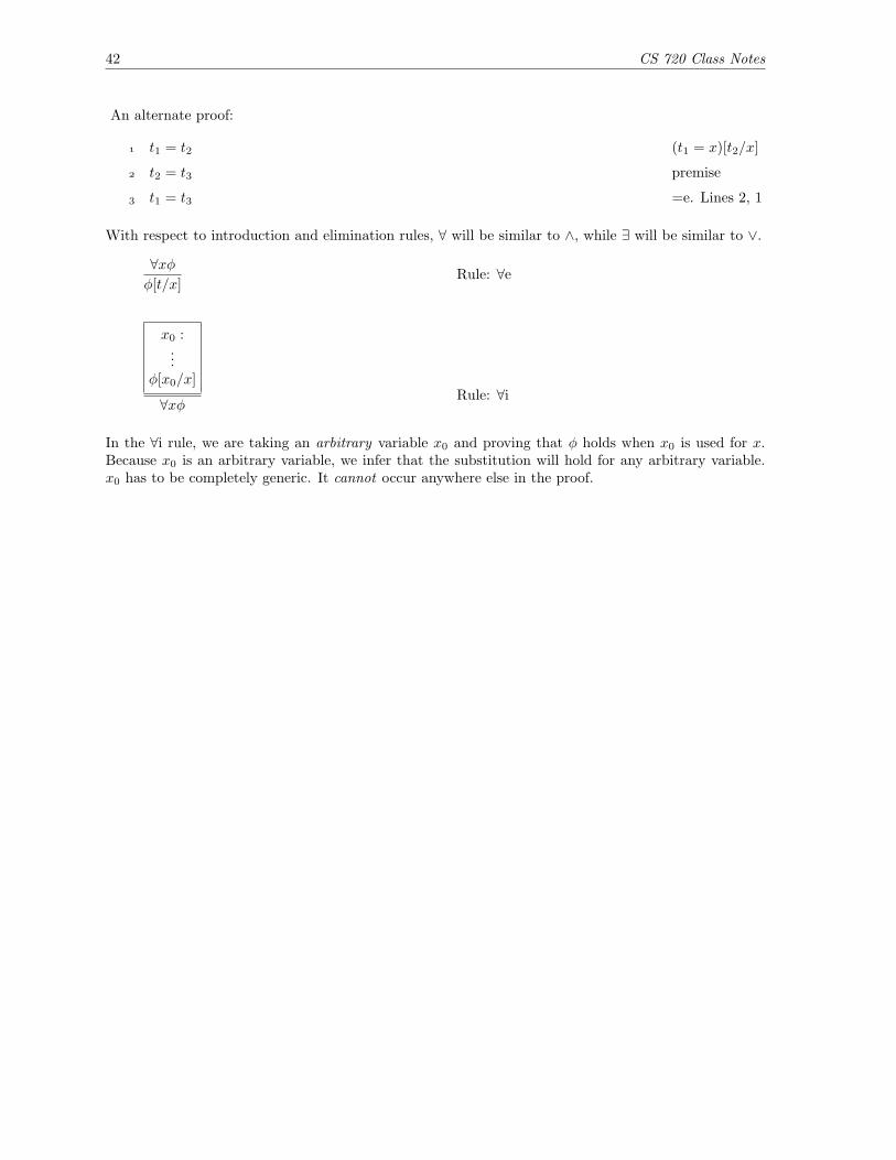
An alternate proof:
t1 = t2 (t1 = x)[t2/x]
t2 = t3 premise
t1 = t3 =e. Lines 2, 1
With respect to introduction and elimination rules, ∀ will be similar to ∧, while ∃ will be similar to ∨.
∀xφφ[t/x]
Rule: ∀e
x0 :...
φ[x0/x]
∀xφRule: ∀i
In the ∀i rule, we are taking an arbitrary variable x0 and proving that φ holds when x0 is used for x.Because x0 is an arbitrary variable, we infer that the substitution will hold for any arbitrary variable.x0 has to be completely generic. It cannot occur anywhere else in the proof.

CS 720 Class Notes 43
2.3 1st Order Logic Notes (H&R, Chapter 2)
Definition 2.3.1: Given a term t, a variable x, and a formula φ, we say that t is free for x in φ if no xleaf in φ occurs in the scope of ∀y or ∃y for any variable y occuring in t.
Restated: if t contains a variable y, then the substitution [t/x] cannot cause y to become bound to aquantifier in φ.
In First-Order logic, the rules =i, and =e for equality are reflexive, symmetric, and transitive.
The rules for ∀xi and ∃xe involve the use of a dummy variable. (Huth and Ryan use x0). The rules fordummy variables are as follows:
• x0 must not exist outside the box.
• x0 cannot be carried outside the box.
∀xφ is similar to φ1 ∧ φ2.
• ∀xφ must prove that φ[x0/x] will hold for every x0 (though we use an arbitrary x0 to prove it).
• φ1 ∧ φ2 must prove that φi holds for every i = 1, 2.

44 CS 720 Class Notes
2.4 Lecture – 2/26/2007
2.4.1 Natural Deduction for Propositional Logic
In our last lecture, we covered the following rules:
∀xφφ[t/x]
Rule: ∀xe
x0
...φ[x0/x]
∀xφRule: ∀xi
Example 2.4.1: Prove P (t),∀x(P (x)→ ¬Q(x)) ` ¬Q(t).
P (t) premise
∀x(P (x)→ ¬Q(x)) premise
P (t)→ ¬Q(t) ∀e. Line 2
¬Q(t) →e. Lines 1, 3
Example 2.4.2: Prove ∀x(P (x)→ Q(x)),∀x(P (x)) ` ∀xQ(x).
∀x(P (x)→ Q(x)) premise
∀x(P (x)) premise
x0 P (x0) ∀e. Line 2
P (x0)→ Q(x0) ∀e. Line 1
Q(x0) →e. Lines 3, 4
∀xQ(x) ∀i. Lines 3–5
2.4.2 Existential Quantifiers
Where ∀ behaves similar to ∧, ∃ behaves similar to ∨. The rules for ∃ are
φ[t/x]∃xφ
Rule: ∃i
x0 φ[x0/x]...χ
χRule: ∃e
Example 2.4.3: Prove ∀xφ ` ∃xφ.
∀xφ premise
φ[x/x] ∀e. Line 1
∃xφ ∃i. Line 2
CS 720 Class Notes 45
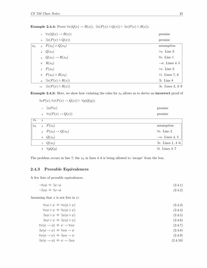
Example 2.4.4: Prove ∀x(Q(x)→ R(x)), ∃x(P (x) ∧Q(x)) ` ∃x(P (x) ∧R(x)).
∀x(Q(x)→ R(x)) premise
∃x(P (x) ∧Q(x)) premise
x0 P (x0) ∧Q(x0) assumption
Q(x0) ∧e. Line 3
Q(x0)→ R(x0) ∀e. Line 1
R(x0) →e. Lines 4–5
P (x0) ∧e. Line 3
P (x0) ∧R(x0) ∧i. Lines 7, 6
∃x(P (x) ∧R(x)) ∃i. Line 8
∃x(P (x) ∧R(x)) ∃e. Lines 2, 3–9
Example 2.4.5: Here, we show how violating the rules for x0 allows us to derive an incorrect proof of
∃xP (x),∀x(P (x)→ Q(x)) ` ∀y(Q(y)).
∃xP (x) premise
∀x(P (x)→ Q(x)) premise
x0
x0 P (x0) assumption
P (x0)→ Q(x0) ∀e. Line 2
Q(x0) →e. Lines 4, 5
Q(x0) ∃e. Lines 1, 4–6.
∀yQ(y) ∀i. Lines 3–7
The problem occurs in line 7; the x0 in lines 4–6 is being allowed to ’escape’ from the box.
2.4.3 Provable Equivalences
A few lists of provable equivalences.
¬∀xφ a` ∃x¬φ (2.4.1)¬∃xφ a` ∀x¬φ (2.4.2)
Assuming that x is not free in ψ:
∀xφ ∧ ψ a` ∀x(φ ∧ ψ) (2.4.3)∀xφ ∨ ψ a` ∀x(φ ∨ ψ) (2.4.4)∃xφ ∧ ψ a` ∃x(φ ∧ ψ) (2.4.5)∃xφ ∨ ψ a` ∃x(φ ∨ ψ) (2.4.6)
∀x(ψ → φ) a` ψ → ∀xφ (2.4.7)∃x(φ→ ψ) a` ∀xφ→ ψ (2.4.8)∀x(φ→ ψ) a` ∃xφ→ ψ (2.4.9)∃x(ψ → φ) a` ψ → ∃xφ (2.4.10)
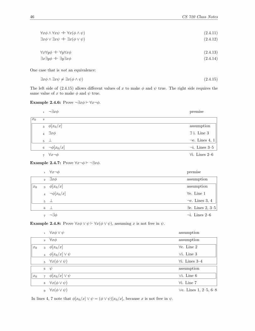
46 CS 720 Class Notes
∀xφ ∧ ∀xψ a` ∀x(φ ∧ ψ) (2.4.11)∃xφ ∨ ∃xψ a` ∃x(φ ∨ ψ) (2.4.12)
∀x∀yφ a` ∀y∀xφ (2.4.13)∃x∃yφ a` ∃y∃xφ (2.4.14)
One case that is not an equivalence:
∃xφ ∧ ∃xψ 6= ∃x(φ ∧ ψ) (2.4.15)
The left side of (2.4.15) allows different values of x to make φ and ψ true. The right side requires thesame value of x to make φ and ψ true.
Example 2.4.6: Prove ¬∃xφ ` ∀x¬φ.
¬∃xφ premise
x0
φ[x0/x] assumption
∃xφ ∃ i. Line 3
⊥ ¬e. Lines 4, 1
¬φ[x0/x] ¬i. Lines 3–5
∀x¬φ ∀i. Lines 2–6
Example 2.4.7: Prove ∀x¬φ ` ¬∃xφ.
∀x¬φ premise
∃xφ assumption
x0 φ[x0/x] assumption
¬φ[x0/x] ∀e. Line 1
⊥ ¬e. Lines 3, 4
⊥ ∃e. Lines 2, 3–5
¬∃φ ¬i. Lines 2–6
Example 2.4.8: Prove ∀xφ ∨ ψ ` ∀x(φ ∨ ψ), assuming x is not free in ψ.
∀xφ ∨ ψ assumption
∀xφ assumption
x0 φ[x0/x] ∀e. Line 2
φ[x0/x] ∨ ψ ∨i. Line 3
∀x(φ ∨ ψ) ∀i. Lines 3–4
ψ assumption
x0 φ[x0/x] ∨ ψ ∨i. Line 6
∀x(φ ∨ ψ) ∀i. Line 7
∀x(φ ∨ ψ) ∨e. Lines 1, 2–5, 6–8
In lines 4, 7 note that φ[x0/x] ∨ ψ = (φ ∨ ψ)[x0/x], because x is not free in ψ.

CS 720 Class Notes 47
Example 2.4.9: Prove ∀x(φ ∨ ψ) ` ∀xφ ∨ ψ.
∀x(φ ∨ ψ) premise
(∀xφ) ∨ ¬(∀xφ) LEM
∀xφ assumption
∀xφ ∨ ψ ∨i. Line 4
¬∀xφ assumption
...
∃x¬φ Proven earlier. Omitted here.
x0 ¬φ[x0/x] assumption
(φ ∨ ψ)[x0/x] ∀e. Line 1
φ[x0/x] assumption
⊥ ¬e. Lines 10, 8
ψ ⊥e. Line 11
ψ assumption
ψ ∨e. Lines 9, 10–12, 13
ψ ∨e. Why??
∀xφ ∨ ψ ∨i. Line 15
∀xφ ∨ ψ ∨i. Lines 2, 3–4, 5–16
More Proofs involving non-free variables
Example 2.4.10: Prove φ a` ∀xφ, where x is not free in φ.
Because x is not free in φ, we can do substitutions without changing φ.
φ premise
x0 φ Copy. Line 1
∀xφ ∀i. Line 2
In the other direction
∀xφ premise
φ ∀e. Line 1
We can do the same thing with the existential quantifier.
Example 2.4.11: Prove φ a` ∃xφ, if x is not free in φ.
φ premise
∃xφ ∃i. (φ = φ[x/x])
In the other direction
∃xφ premise
x0 φ[x0/x] assumption (φ[x0/x] = x)
φ ∃e.

48 CS 720 Class Notes
If x is not free in φ, we could even prove
∃xφ a` ∀xφ
2.4.4 Semantics in First-Order Logic
Suppose we are given
∃x∀y P (x, y) � ∀y∃xP (x, y)
x and y are independant, but both must come from some domain of values. Similarly P also has ameaning.
For first-order logic, “valid” means that the truth semantics hold under any model.
CS 720 Class Notes 49
2.5 Lecture – 2/28/2007
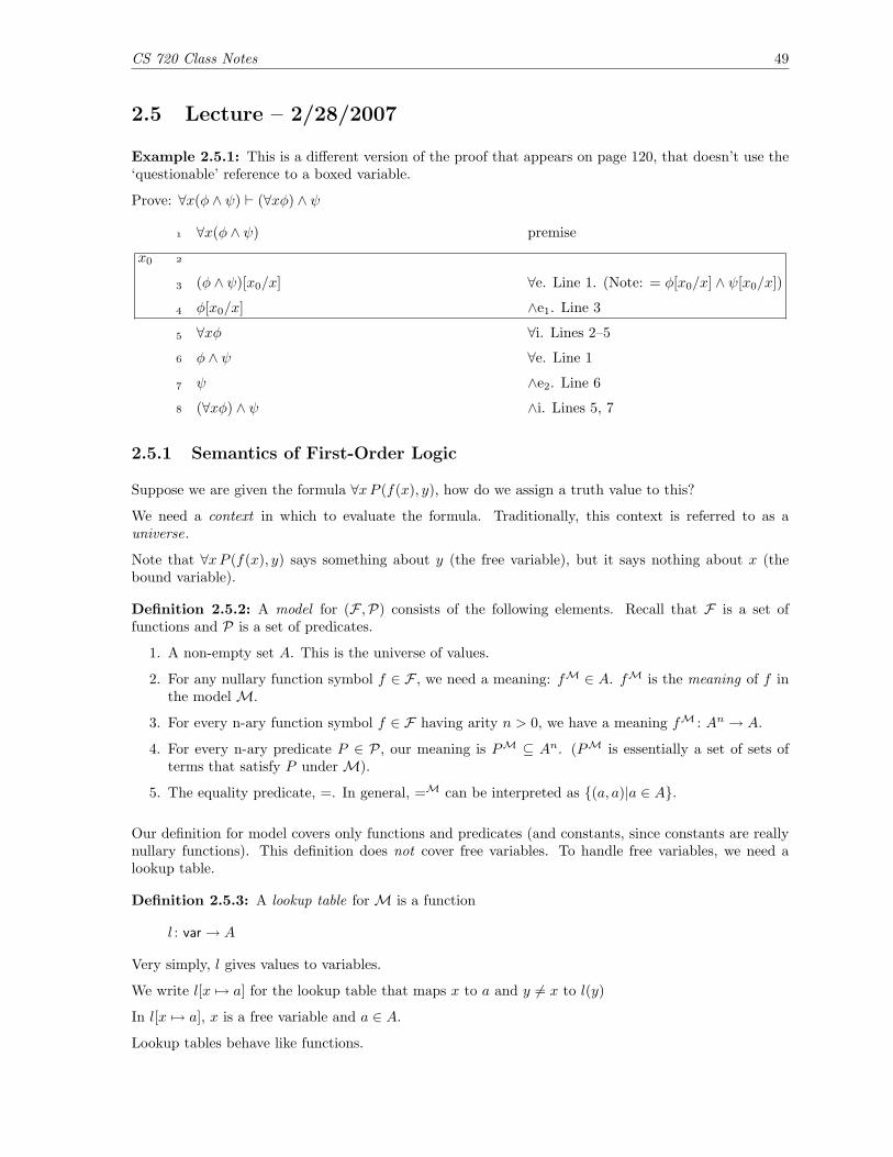
Example 2.5.1: This is a different version of the proof that appears on page 120, that doesn’t use the‘questionable’ reference to a boxed variable.
Prove: ∀x(φ ∧ ψ) ` (∀xφ) ∧ ψ
∀x(φ ∧ ψ) premise
x0
(φ ∧ ψ)[x0/x] ∀e. Line 1. (Note: = φ[x0/x] ∧ ψ[x0/x])
φ[x0/x] ∧e1. Line 3
∀xφ ∀i. Lines 2–5
φ ∧ ψ ∀e. Line 1
ψ ∧e2. Line 6
(∀xφ) ∧ ψ ∧i. Lines 5, 7
2.5.1 Semantics of First-Order Logic
Suppose we are given the formula ∀xP (f(x), y), how do we assign a truth value to this?
We need a context in which to evaluate the formula. Traditionally, this context is referred to as auniverse.
Note that ∀xP (f(x), y) says something about y (the free variable), but it says nothing about x (thebound variable).
Definition 2.5.2: A model for (F ,P) consists of the following elements. Recall that F is a set offunctions and P is a set of predicates.
1. A non-empty set A. This is the universe of values.
2. For any nullary function symbol f ∈ F , we need a meaning: fM ∈ A. fM is the meaning of f inthe model M.
3. For every n-ary function symbol f ∈ F having arity n > 0, we have a meaning fM : An → A.
4. For every n-ary predicate P ∈ P, our meaning is PM ⊆ An. (PM is essentially a set of sets ofterms that satisfy P under M).
5. The equality predicate, =. In general, =M can be interpreted as {(a, a)|a ∈ A}.
Our definition for model covers only functions and predicates (and constants, since constants are reallynullary functions). This definition does not cover free variables. To handle free variables, we need alookup table.
Definition 2.5.3: A lookup table for M is a function
l : var→ A
Very simply, l gives values to variables.
We write l[x 7→ a] for the lookup table that maps x to a and y 6= x to l(y)
In l[x 7→ a], x is a free variable and a ∈ A.
Lookup tables behave like functions.

50 CS 720 Class Notes
2.5.2 Evaluating Formulas With Models
In first-order logic, the symbol � is overloaded. One meaning is semantic entailment. The other meaninghas to do with the evaluation of a formula in a model.
We write
M �l φ
to mean that φ evaluates to T in the model M under the lookup function l.
Again, M is a model, l is a lookup table, and φ is a formula.
Let’s build up a definition of evaluation.
• Let tM,l denote the value of the term t in M under l.
• xM,l = l(x), where x is a (free) variable.
• If f is a nullary function (constant), then fM,l = fM.
• f(t1, . . . , tn)M,l = fM(tM,l1 , . . . , tM,l
n )
That covers evaluation of terms. Now, lets move on to formulas.
• M �l P (t1, . . . , tn) IFF (tM,l1 , . . . , tM,l
n ) ∈ PM.
• M �l ¬φ IFF not M �l φ.
• M �l φ ∨ ψ IFF M �l φ or M �l ψ
• M �l φ ∧ ψ IFF M �l φ and M �l ψ
• M �l φ→ ψ IFF not M �l φ or M �l ψ
• M �l ∀xφ IFF for all a ∈ A, M �l[x 7→a] φ
• M �l ∃xφ IFF for some a ∈ A, M �l[x 7→a] φ
Let’s go back to our earlier question: what does ∀xP (f(x), y) mean? Using our definitions:
For all a ∈ A, M �l[x 7→a] makes P (f(x), y) true.For all a ∈ A, (fM(a), l(y)) ∈ PM.
Suppose we had two lookup tables l, l′, and that these two tables agree on all free variables of φ. Then
M �l φ IFF M �l′ φ
Definition 2.5.4: φ is a sentence if φ has no free variables.
Suppose φ is a sentence. Then, either M �l φ for all l, or M 2l φ for all l.
Why is this the case? Lookup tables apply to free variables only. If φ is a sentence, then φ has no freevariables, so it doesn’t matter which lookup table we use. Every lookup table is equivalent!
Put another way M �l φ is equivalent to M � φ. If φ is a sentence, then the lookup table is irrelevant.
2.5.3 Semantic Entailment in First-Order Logic
As noted, � is also used to represent semantic entailment in first-order logic.
We write Γ � ψ to mean that “Gamma entails psi”. As before, we use the convention of using Γ torepresent a set of formulas.
If M �l φ for all φ ∈ Γ, then M �l ψ.
CS 720 Class Notes 51
To reiterate the overloaded notation:
Γ � ψ LHS is a set of formulasM �l ψ LHS is a model
Definition 2.5.5: We say that ψ is satisfiable if there are M, l such that M �l ψ.
Definition 2.5.6: We say that ψ is valid if M �l ψ for all M, l.
This is a very big statement. In the realm of models, ‘all’ really means ‘every thing you could possiblythink of’.
Definition 2.5.7: Γ = φ1, . . . , φn is satisfiable if there is M, l such that M �l φ for all φ ∈ Γ.
Question: if Γ = ∅, is Γ still satisfiable? Yes, Γ = ∅ is satisfiable.
2.5.4 Soundness and Completeness of First-Order Logic
Recall,
Soundness A syntactic notion. If Γ ` φ, then Γ � φ. Note that Γ may be a finite set of formulas, or Γmay be an infinite set of formulas.
Completeness If Γ � φ, then Γ ` φ.
Soundness is the more important quality. Soundness allows us to trust what we have proven syntactically.
Soundness and Completeness hold for First-Order logic. (We’re not going to explore a proof here, butthe principles hold).
2.5.5 The Validity Problem
The validity problem is as follows: Given a formula φ, is φ valid? (i.e. is � φ true?)
In propositional logic, validity is a decidable problem. We can construct a truth table for the givenformula and see if all rows evaluate to T. Although there’s no efficient way to determine validity forpropositional logic, it’s still a computable problem.
In first-order logic, validity is not decidable. Huth and Ryan give a proof by reduction from the PostCorrespondence Problem.
Post Correspondence Problem
In the post correspondence problem, we are given a n dominos
s1t1· · · sn
tn(2.5.1)
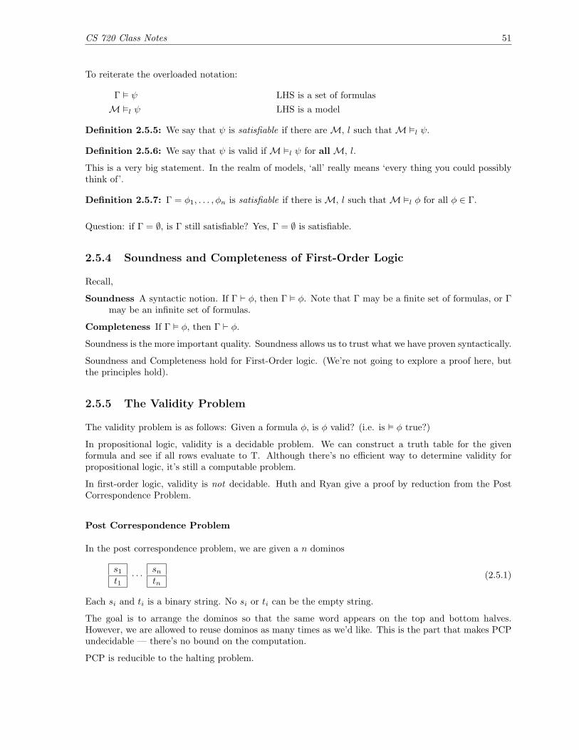
Each si and ti is a binary string. No si or ti can be the empty string.
The goal is to arrange the dominos so that the same word appears on the top and bottom halves.However, we are allowed to reuse dominos as many times as we’d like. This is the part that makes PCPundecidable — there’s no bound on the computation.
PCP is reducible to the halting problem.
52 CS 720 Class Notes
To show that validity is not decidable, we will reduce PCP to validity. This will show validity forfirst-order logic to be undecidable. (A solution to the validity problem would allow us to solve PCP bytransforming an instance of the PCP into the validity problem).
Given an instance of the PCP (2.5.1), we will construct a formula ψ such that the PCP instance has asolution IFF ψ is valid.
Our model description for ψ
A = {0, 1}∗
f0(w) = w0 append 0 to wf1(w) = w1 append 1 to wP (s, t) = s = t s = s1, . . . , sn, t = t1, . . . , tn
Representing a string with f0 and f1 will involve a fair amount of recursion. As a notational convenience,let
fb1...bk= fbk
(fbk−1(fbk−2(· · · fb1(e) · · · )))
[to be continued next lecture]
CS 720 Class Notes 53
2.6 Lecture – 3/5/2007
2.6.1 First-Order Logic and the Post Correspondence Problem
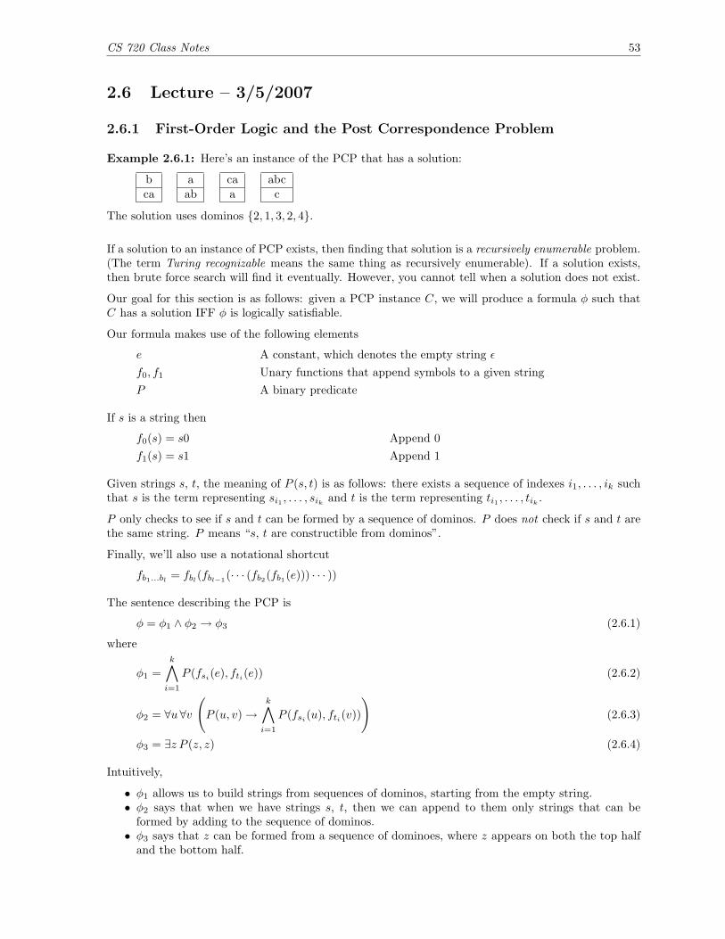
Example 2.6.1: Here’s an instance of the PCP that has a solution:
bca
aab
caa
abcc
The solution uses dominos {2, 1, 3, 2, 4}.
If a solution to an instance of PCP exists, then finding that solution is a recursively enumerable problem.(The term Turing recognizable means the same thing as recursively enumerable). If a solution exists,then brute force search will find it eventually. However, you cannot tell when a solution does not exist.
Our goal for this section is as follows: given a PCP instance C, we will produce a formula φ such thatC has a solution IFF φ is logically satisfiable.
Our formula makes use of the following elements
e A constant, which denotes the empty string εf0, f1 Unary functions that append symbols to a given stringP A binary predicate
If s is a string then
f0(s) = s0 Append 0f1(s) = s1 Append 1
Given strings s, t, the meaning of P (s, t) is as follows: there exists a sequence of indexes i1, . . . , ik suchthat s is the term representing si1 , . . . , sik and t is the term representing ti1 , . . . , tik .
P only checks to see if s and t can be formed by a sequence of dominos. P does not check if s and t arethe same string. P means “s, t are constructible from dominos”.
Finally, we’ll also use a notational shortcut
fb1...bl= fbl
(fbl−1(· · · (fb2(fb1(e))) · · · ))
The sentence describing the PCP is
φ = φ1 ∧ φ2 → φ3 (2.6.1)
where
φ1 =k∧i=1
P (fsi(e), fti(e)) (2.6.2)
φ2 = ∀u∀v
(P (u, v)→
k∧i=1
P (fsi(u), fti(v))
)(2.6.3)
φ3 = ∃z P (z, z) (2.6.4)
Intuitively,
• φ1 allows us to build strings from sequences of dominos, starting from the empty string.• φ2 says that when we have strings s, t, then we can append to them only strings that can be
formed by adding to the sequence of dominos.• φ3 says that z can be formed from a sequence of dominoes, where z appears on both the top half
and the bottom half.

54 CS 720 Class Notes
A Proof that This Reduction Works
Part One: Suppose that � φ is valid (where φ = φ1 ∧φ2 → φ3). Then φ must be valid for our model ofthe Post Correspondence Problem. We need to give a formal defintion of our model that demonstratesits φ’s validity.
Let
M = (A, eM, fM0 , fM1 , PM)
where
A = {0, 1}∗
eM = ε
fM0 (w) = w0
fM1 (w) = w1
PM(s, t) = {(s, t) | there is a sequence of indices i1, . . . , im such that s = si1 , . . . , sim
and t = ti1 , . . . , tim}
If � φ is valid, then M � φ is valid.
If t is a variable-free term, then (fs(t))M = tM · s. So M � φ1.
If the pair (s, t) ∈ PM, then the pair (ssi, tti) ∈ PM for i = 1, . . . , k. So, M � φ2.
Since φ1 ∧ φ2 → φ3, and φ1 ∧ φ2 holds, φ3 must hold as well. The definitions of φ3 and PM says thatthere is a solution to the PCP instance C.
So, if φ is valid, then then C has a solution.
Part Two. Suppose C has a solution. We must show that φ is valid for any model M′
By our definition of φ, ifM′ 2 φ1 orM′ 2 φ2 then we are done — φ is vacuously valid. The harder partis handling when M′ � φ1 ∧ φ2. In that case, we must verify M′ � φ3 as well.
We do this by interpreting binary strings in the domain of values A′ for the model M′. Let us define afunction
interpret : {0, 1}∗ → A
interpret(ε) = eM′
interpret(s0) = fM′
0 (interpret(s))
interpret(s1) = fM′
1 (interpret(s))
interpret(b1 . . . bl) = fM′
bl(fM
′
bl−1(· · · (fM
′
b1 (eM′)) · · · ))
Since, M′ � φ1, we can conclude that
(interpret(si), interpret(ti)) ∈ PM′
for i = 1, . . . , k
Since M′ � φ2, we can conclude that
(interpret(ssi), interpret(tti)) ∈ PM′
for i = 1, . . . k
CS 720 Class Notes 55
Starting with (s, t) = (si1 , ti1), we can repeatedly apply the previous formula to obtain
(interpret(si1 . . . sin), interpret(ti1 . . . tin)) ∈ PM′
Since si1 . . . sin and ti1 . . . tin form a solution to C, they are equal. Therefore, interpret(si1 . . . sin) andinterpret(ti1 . . . tin) are the same elements in A′. Therefore ∃z P (z, z) is in M′ and M′ � φ3.
This shows a reduction from PCP to the validity problem for first-order logic. Because PCP is notdecidable, the validty problem for first-order logic is not decidable.
2.6.2 Implications of the Undecidability of the Validity Problemfor First-Order Logic
Having shown that validity is undecidable for first-order logic, we may conclude two additional things:
1. φ is satisfiable IFF ¬φ is valid. Because we can’t compute validity, we can’t compute satisifiabilityeither.
2. � φ IFF ` φ. Because validity is not computable, provability is not computable either.
Validity is recursively enumerable. To check validity, one must consider all finite models and all infinitemodels. � φ is R.E. because of soundness and completeness. We can try all possible proofs. If we find aproof, soundness assures us that the proof will hold.
The set of non-valid formulas is not recursively enumerable. If the set of non-valid formulas were RE,then validity would be recursive (aka, Turing Computable). A set is recursive IFF the set and itscompliment are recursively enumerable.
As an aside, there are formulas of first-order logic that are not valid, but are true for all finite structures.Simply enumerating all possible finite structures is not sufficient to test for validity.
2.6.3 Expressiveness of First-Order Logic
First-Order logic is pretty powerful, but there are concepts it cannot express.
Theorem 2.6.2 (Compactness Theorem): If Γ is a set of sentences and all finite subsets of Γ aresatisfiable, then Γ is satisfiable.
Proof: Suppose that Γ were unsatisfiable. Because Γ is unsatisfiable, then Γ � ⊥ and Γ ` ⊥ (bycompleteness).
Let ∆ be some finite subset of Γ. We have ∆ ` ⊥, since proofs have finite length. Because ∆ ` ⊥,soundness and completeness tell us that ∆ � ⊥.
∆ � ⊥ contradict the assumption that all sentences in Γ are consistent; Γ must be satisifiable.
Theorem 2.6.3 (Lowenheim-Skolem Theorem): If Γ is a set of sentences, and for all n ≥ 1, Γ has amodel M with at least n elements, then Γ has a model with infinitely many elements.
The phrase “for all n ≥ 1, Γ has a model M” refers to M � φ for all φ ∈ Γ.
The phrase “a model M with at least n elements”, means that the universe A of M has at least nelements.
56 CS 720 Class Notes
2.7 Chapter 2.4 Notes
2.7.1 Semantics of Predicate Logic
It’s generally easy to show Γ ` ψ — just write a proof. It’s much harder to show that no proof exists.
Γ � ψ is just the opposite. It’s generally easy to show a counterexample where Γ 2 ψ. Showing Γ � ψfor all possible models M is usually difficult.
The evaluation of any first-order logic formula requires a universe of values.
Definition 2.7.1 (Model): A model for (F ,P) is
M = (A, cM, fM, PM)
where
• A is a universe of concrete values• cM. For each nullary function (constant) we need a concrete a ∈ A that the constant stands for.• fM. For each n-ary function fM : An → A, we need a concrete function definition.• PM. For each n-ary predicate, we need a set of n-ary tuples that satisfy the predicate. For an
n-ary predicate P , PM ⊆ An.
f and P are simply symbols. By contrast, fM is a concrete function and PM is a concrete relation.The notion of “model” is very liberal and very open-ended.
There is one area that our definition of model does not address: free variables. To handle free variables,we need a lookup table
l : var→ A
Lookup tables are also denoted by l[x 7→ a]. l[x 7→ a] means that l maps x to a ∈ A, and for all y 6= x, lmaps y to l(y).
If a first-order logic formula is a sentence, then validity holds (or does not hold) irrespective of thelook-up table. If φ is a sentence, then φ has no free variables; if φ has no free variables, then the lookuptable is irrelevant.
The semantics of first-order logic impose a special meaning on the symbol =, which we denote =M.(a, b) is in the relationship =M IFF a and b are the same elements of A.
2.7.2 Semantic Entailment (Section 2.4.2)
Definition 2.7.2 (Semantic Entailment): Let Γ = φ1, . . . , φn. We say that Γ semantically entails ψ, or
φ1, . . . , φn � ψ
IFF ψ is true whenever all φ1, . . . , φn ∈ Γ are true.
Some useful rules for semantic entailment.
1. Γ � ψ holds IFF for all modelsM and lookup tables l, wheneverM �l φ holds for all φ in Γ, thenM �l ψ holds as well.
2. Formula ψ is satisfiable IFF there is some model M and some environment l such that M �l ψholds.
CS 720 Class Notes 57
3. Formula ψ is valid IFFM �l ψ holds for all modelsM and environments l in which we can checkψ.
4. The set Γ is consistent or satisfiable IFF there is a modelM and a lookup table l such thatM �l φholds for all φ ∈ Γ.
2.7.3 Decidability of First-Order Logic
Establishing M � ψ is undecidable if the universe of M is infinite. If the universe is infinite, there’s noway that we can check each value.
Determining whether φ1 . . . φn � ψ is also an undecidable problem. Validity requires entailment to holdunder all possible models. Because there are an infinite number of potential models, we cannot checkthis programatically either.
By contrast, validity and satisfiability are decidable problems in propositional logic: construct a truthtable and examine it. This is not an efficient approach, but it can be done programatically.
2.7.4 Soundness and Completeness
As with predicate logic,
φ1, . . . , φn ` ψ IFF φ1, . . . , φn � ψ (2.7.1)
Soundess and completeness hold for first-order logic.
58 CS 720 Class Notes
2.8 Lecture – 3/7/2007
2.8.1 Lowenheim-Skolem Theorem
Last time we discussed the Lowenheim-Skolem Theorem (See Theorem 2.6.3, page 55). If Γ is a set ofsentences and for all n ≥ 1 Γ has a model of size n, then Γ has an infinite model.
The phrase “Γ has a model of size n” means that there is a modelM = (A, . . .) and for all φ ∈ Γ,M � φand |A| ≥ n.
Indirectly, this theorem is saying that first-order logic gives us no way to say “the universe is finite”.
Proof (Lowenheim-Skolem Theorem): For all n ≥ 1, let φn be the formula
∃x1 ∃x2 . . . ∃xn
n∧i 6=j
¬(xi = xj)
(2.8.1)
Equation (2.8.1) states that there are at least n elements in our universe.
Let ∆ = Γ ∪ {φn | n ≥ 1}. ∆ is adding n formulas to the set Γ.Let ∆′ be a finite subset of ∆.Let m = max{n | φn ∈ ∆′}.Let M be a model for Γ with at least m elements.
Because M is a model for ∆, M is also a model for ∆′.
By the compactness theorem, ∆ has a model M′ which is an infinite model of Γ.
2.8.2 First-Order Logic and Directed Graphs
The compactness theorem also allows us to prove some things about first-order logic and directed graphs.
A directed graph is a set of vertices and edges: G = (V,E).
E is equivalent to a binary predicate that states whether two nodes are connected. Let us represent theset E with the logical predicate R.
A specific instance of a graph will serve as a model.
Graphs are commonly used in program verification. Nodes represent states and edges represent statetransitions. Typical verification problems ask the question “is there a path from a good state to a badstate?”.
We define our relation R
R = {(u, v) | there is a path from u to v}
We refer to R as the reachability relation.
R is the reflexive, transitive closure of the set of edges. (Reflexive, because we consider (u, u) as a pathof length zero from u to itself).
The question: is reachability expressible in predicate logic?
More formally, is there a formula φ with a single binary predicate R and free variables u, v such thatfor all models M and lookup tables l, M �l φ?
(Note: because we’re working with free variables, we’re actually concerned about paths between l(u)and l(v)).
CS 720 Class Notes 59
The answer: no such formula exists. There is no formula in predicate logic that can show reachabilityfor all directed graphs.
If such a formula did exist, it would have the form
φ = (u = v) ∨R(u, v) ∨ ∃x (R(u, x) ∧R(x, v)) ∧ . . .
The formula would be infinitely long, which predicate logic doesn’t allow. Allowing infinitely longformulas would invalidate the compactness theorem, and invalidating the compactness theorem wouldinvalidate soundness and completeness.
Theorem 2.8.1: Reachability is not expressible in predicate logic: there is no formula φ, whose onlyfree variables are u and v and whose only predicate symbol (of arity 2) is R, such that φ holds IFF thereis a path in that graph from the node associated to u to the node associated to v.
Proof: Suppose there were such a formula φ. Let c and c′ be constants. Let φn be the formulaexpressing that there is a path of length n from u to v.
φ0 = c = c′
φ1 = R(c, c′)φ2 = ∃x (R(u, x) ∧R(x, v))
...φn = ∃x1 . . . ∃xn−1 (R(c, x1) ∧R(x1, x2) ∧ · · · ∧R(xn−1, c
′))
Let us define
∆ = {¬φi | i ≥ 0} ∪ {φ[c/u][c′/v]}
∆ is unsatisfiable: {¬φi | i ≥ 0} says that no path exists, while {φ[c/u][c′/v]} says that a path doesexist.
However, every finite subset of ∆ is satisfiable since there are paths of any finite length. Therefore,by the compactness theorem, ∆ is satisfiable. This is a contradiction, since ∆ was designed to be anunsatisfiable formula. Therefore, no such φ exists.
So we see that first-order logic is powerful, but it has its shortcomings. It’s powerful enough to enter therealm of undecidability (the validity and satisfiability problems), but there are some simple problemsthat it cannot express (reachability).
2.8.3 Second-Order Logic
First-order logic cannot express reachability, but second-order logic can. Where first-order logic gives usfreedom over individual objects, second-order logic gives us freedom over predicates.
Second-order logic has no compactness theorem.
2.8.4 Existential Second-Order Logic
Existential Second-Order Logic formulas have the form
∃P φ
Where P is a predicate symbol and φ is a propositional logic, or first-order logic formula.
60 CS 720 Class Notes
Let M be a model for the language of (φ− P ).
Let T ⊆ A×A. MT will be a full model for φ, where PMT = T .
We will have M �l ∃P φ IFF there is a T ∈ A×A with MT �l φ.
Non-Reachability can be expressed in second-order logic as
∃P∀x∀y∀z (C1 ∧ C2 ∧ C3 ∧ C4)
where each Ci is a horn clause
C1 = P (x, x) (2.8.2)C2 = P (x, y) ∧ P (y, z)→ P (x, z) (2.8.3)C3 = P (u, v)→ ⊥ (2.8.4)C4 = R(x, y)→ P (x, y) (2.8.5)
C1 states that P is reflexive.C2 states the P is transitive.C3 ensures that there is no P path from u to v.C4 says that any R edge is also a P edge.
Which is a good definition of non-reachability in a directed graph. It expresses reflexivity and transitivity,and also that you cannot get from u to v.
2.8.5 Universal Second-Order Logic
Formulas of universal second-order logic have the form
∀P φ
Where existential second-order logic allowed to express non-reachability, universal second-order logicallows us to express reachability.
φ = ∀P∃x∃y∃z(¬C1 ∨ ¬C2 ∨ ¬C3 ∨ ¬C4) (2.8.6)
where each Ci is as defined in (2.8.2) - (2.8.5).
Theorem 2.8.2: Let M = (A,RM) be any model. Then formula (2.8.6) holds under lookup table l inM IFF l(v) is R-reachable from l(u) in M.
Proof: Case 1. Suppose that M � φ (for φ in (2.8.6)) holds for all interpretations of M. Then italso holds for the model where P is the reflexive transitive closure of R.
In the model where P is the reflexive transitive closure of R, only the clause ¬C3 will hold. But thismeans that M � P (u, v) has to hold, so there is path of finite length from l(u) to l(v).
Case 2. Let l(v) be R-reachable from l(u) in M. For any interpretation where P is not reflexive, nottransitive, or does not contain R, φ will still hold. One of the clauses ¬C1, ¬C2 or ¬C4 will be true.
If the interpretation has P being the reflexive transitive closure of R, then P will certainly contain R.The clauses ¬C1, ¬C2, ¬C4 will be false, but ¬C3 will be true, because (l(u), l(v)) is in the reflexivetransitive closure by assumption. Therefore φ still holds.

CS 720 Class Notes 61
2.8.6 Program Verification
There are two schools of program verification: model-based and proof-based.
Model-Based Verification Model-based verification usesM � φ, but assumes thatM is finite. IfMis finite, then M � φ is decidable. You can try every possible combination.
Model-based verification is retrospective. You do it after you’ve constructed the model.
Proof-Based Verification Proof-based verification relies on soundness and completeness. We try toestablish φ1, . . . , φn � φ by constructing a syntactic proof for φ1, . . . , φn ` φ.
Proof-based verification is prospective. You can do it before the model has been constructed. Thiscan be help you decide when the model is sufficient. If you can prove φ, you’re done.
Part 3
Program Verification
3.1 Lecture – 3/12/2007
3.1.1 An Introduction to Verification
There are three ingredients in program verification:
1. A means of modeling the system. Typically this is mathematical model.
2. Specifying a language for system properties.
3. A way of verifying that the model matches (or fails to match) the desired program behavior. (Averification method).
Verification methods can be classified according to several criteria:
• Proof-based vs. Model Based.
Proof-based verification models a system by a set of formulas, Γ. The specification is anotherformula φ. Verification involves finding a proof for Γ ` φ in some formal system. Assuming thatthe formal system is sound, we can determine whether Γ � φ.
Model-based methods use a model M. The specification is a formula φ. Verification involvesshowing that M � φ.
If M is a finite model, then the verification problem is decidable (but not necessarily efficient).
• Degree of Automation.
The verification process may be (1) fully-automatic, (2) computer assisted or (3) manual.
Fully-automatic verification works better for model-based systems.
Fully-manual verification works better for proof-based systems.
• Full Verification vs. Property Verification.
Full Verification tries to develop a complete specification of the program: what must be true aboutits inputs, what must be true about its outputs, as well as the details of the program’s behavior.While this method may be practical for small programs, it is usually impractical for medium tolarge programs.
Property Verification does not try to produce a complete description of the program. Instead, itfocuses on certain aspects of the program’s behavior.
62

CS 720 Class Notes 63
Property Verification is weaker than full verification, but easier to do. With property verification,you can at least make assertions about some aspects of the system.
• Intended Domain.
What type of program are you verifying? Is it sequential or concurrent? Is it reactive or termi-nating?
• Pre-development vs. Post-development.
When is the verification process applied? It’s preferably to apply verification earlier in the devel-opment process, when mistakes are less costly to rectify.
3.1.2 Model-Checking
We will focus on model checking as a verification mechanism. Some characteristics of model checkingare:
• It’s model-based• Fully-automated• Uses property verification• It applies to the domain of concurrent, reactive systems• It’s done in Post-development• It’s based in linear temporal logic (LTL). LTL is a form of logic that involves time.• The model will be based on a transition system.• If the model is inconsistent (i.e., ifM 2 φ), then the verification process will produce a counterex-
ample.
Alloy is a Hybrid model verifier. It limits the size of the model search space, under the assumption thatcounterexamples can usually be found in small models.
3.1.3 Temporal Logic Systems
Temporal logics are formal logic systems that involve time. We’ll be concerned with two temporal logicsystems:
1. Linear Temporal Logic. LTL assumes that time proceeds linearly along a single path. LTLallows a single ’next’ step in time.
S1 -> S2 -> S3 -> ...
2. Branching Temporal Logic. Branching temporal logic allows multiple ’next’ steps. For example:
-------> S4 ------> ...|
-----> S2 ---->|| |
S1-->| -------> S3 ------> ...|----------- S5 -------> ...
We’ll focus on Linear Temporal Logic first.
3.1.4 Linear Temporal Logic
LTL views time as a sequence of states, extending (perhaps infinitely far) into the future. There maybe several possible paths, but only path will be realized.

64 CS 720 Class Notes
LTL makes use of atoms: p, q, r, etc. Atoms stand for facts that may be true or false in the system.For example, “printer lj2 is busy”, “process X is suspended”, etc.
In EBNF, the syntax for LTL is as follows:
φ ::=>| ⊥| p where p is an atom| (¬φ) where φ is any LTL formula| (φ ∧ φ) and the other φ is any other LTL formula| (φ ∨ φ)| (φ→ φ)| (X φ)| (F φ)| (G φ)| (φ U φ)| (φ W φ)| (φ R φ)
The symbols X, F, G, U, W, and R are called temporal connectives. Their names are
Connective NameX NextF FutureG GlobalU UntilW Weak UntilR Release
The precedence order of LTL connectives is
¬,X,F,G unary connectivesU,W,R LTL binary connectives∧,∨→
3.1.5 Semantics of Linear Temporal Logic
LTL is based on a transition system. A transition system consists of states (static structures) andtransitions (dynamic structures).
Definition 3.1.1 (Transition System): A transition system,M = (S,→, L) is a set of States S, a binarytransition relation →, and a labeling function L.
→ is a binary relation on S. For every s ∈ S, there will be some s′ ∈ S such that s→ s′. Dead ends arenot allowed in this transition system.
The labeling function, L : S → P(atoms). For a state s, L(s) contains the set of atoms that are true ins.
Example 3.1.2: Figure 3.1 shows an LTL transition system. In this system,
• S0 is the starting state.
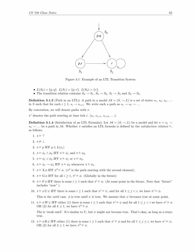
CS 720 Class Notes 65
p,q0
S2S1
p,r r
S
Figure 3.1: Example of an LTL Transition System
• L(S0) = {p, q}. L(S1) = {p, r}. L(S2) = {r}.• The transition relation contains S0 → S1, S0 → S2, S1 → S2 and S2 → S2.
Definition 3.1.3 (Path in an LTL): A path in a model M = (S,→, L) is a set of states s1, s2, s3, . . .in S such that for each i ≥ 1, si → si+1. We write such a path as s1 → s2 → . . .
By convention, we will denote paths with π.
πi denotes the path starting at time tick i. (si, si+1, si+2, . . .).
Definition 3.1.4 (Satisfaction of an LTL Formula): Let M = (S,→, L) be a model and let π = s1 →s2 → . . . be a path in M. Whether π satisfies an LTL formula is defined by the satisfaction relation �,as follows.
1. π � >
2. π 2 ⊥
3. π � p IFF p ∈ L(s1)
4. π � φ1 ∧ φ2 IFF π � φ1 and π � φ2.
5. π � φ1 ∨ φ2 IFF π � φ1 or π � φ2.
6. π � φ1 → φ2 IFF π � φ2 whenever π � φ1.
7. π � Xφ IFF π2 � φ. (π2 is the path starting with the second element).
8. π � Gφ IFF for all i ≥ 1, πi � φ. (Globally in the future)
9. π � Fφ IFF there is some i ≥ 1 such that πi � φ. (At some point in the future. Note that “future”includes “now”.)
10. π � φUψ IFF there is some i ≥ 1 such that πi � ψ, and for all 1 ≤ j < i, we have πj � φ.
This is the until case. φ is true until ψ is true. We assume that ψ becomes true at some point.
11. π � φWψ IFF either (1) there is some i ≥ 1 such that πi � ψ and for all 1 ≤ j < i we have πj � φOR (2) for all k ≥ 1, we have πk � φ.
The is ‘weak until’. It’s similar to U, but ψ might not become true. That’s okay, as long as φ staystrue.
12. π � φRψ IFF either (1) there is some i ≥ 1 such that πi � φ and for all 1 ≤ j ≤ i, we have πj � ψ,OR (2) for all k ≥ 1 we have πk � ψ.

66 CS 720 Class Notes
Here, we say that “φ releases ψ”. ψ must be true up until (and including) the moment where φbecomes true.
R is the dual of U. φRψ ≡ ¬(¬φU¬ψ).
NOTE: in LTL, “future” includes all time steps ≥ i, including i itself.
Also note: φWψ ≡ φUψ ∨Gφ.
If s ∈ S, M, S � φ IFF π � φ for all paths π starting at state S.
3.1.6 Some Examples of LTL formulas
• � G p→ p. This formula is valid. If p holds globally, then p holds in the first state.
• � p→ F p. This is valid, because F includes the present, as well as future states.
• � p → qU p. Valid, but vacuously. If p holds at s1, then we can say q holds until s1. (Vacuous,because there are no points before si).
• 2 p→ pR q. Always false. If p is the first state in the path, then q cannot hold before p does.
• G¬(started ∧ ¬ready). Globally, we cannot be in a started state unless we are in a ready state.
• G(requested → F enabled). If a service is requested, then it must become enabled. This includesbecoming enabled at the time of the request.
• G enabled. Enabled forever, starting now
• F G enabled. Enabled forever, starting at some point in the future.
• G F enabled. Enabled infinitely often. (Allows transitions from enabled to not enabled, back toenabled again).
For next class, try to find an LTL expression that means “If running, then enabled at some point before”.(i.e. - the service goes from not running to running, and becomes enabled at the point where it becomesrunning).

CS 720 Class Notes 67
3.2 Lecture – 3/14/2007
3.2.1 Linear Temporal Logic
Last lecture, we asked how to say “if you’re running at a state (but not at the previous state), thenyou’re enabled”. In LTL, we say this as
G((¬running ∧X running)→ X enabled)
Review:
• F Gφ means “φ will be true forever, starting at some point in the future”.
• G Fφ means “φ is true infinitely often”.
• F Gφ→ G Fφ
What can’t be expressed in linear temporal logic? LTL considers only one path through time; it doesnot have a concept for branching.
Suppose you wanted to say “From any reachable state, you can reach a restart state”. This is like saying“From any reachable state, there exists a path to a restart state”. Consider the transition system inFigure 3.2. This transition system contains two reachable states; the state where restart = T is reachable
restart
1s2s
Figure 3.2: A simple Transition System
from either.
We could try to describe this as G(F restart). But that doesn’t quite work. We might stay at S1 foreverwithout reaching S2.
Statements of the form “There exists a path” are usually not expressible in LTL. But sometimes onecan get around this by using negation (∃xφ ≡ ¬∀x¬φ).
When we say an LTL expression is true, it must be true regardless of any branch chosen.
3.2.2 Equivalences in LTL
G acts like ∀ (or ∧).F acts like ∃ (or ∨).
Some equivalences:
¬Gφ ≡ F¬φ G, F are duals (3.2.1)¬Fφ ≡ G¬φ (3.2.2)¬Xφ ≡ X¬φ X doesn’t have a dual (3.2.3)
¬(φUψ) ≡ ¬φR¬ψ U and R are duals (3.2.4)¬(φRψ) ≡ ¬φU¬ψ (3.2.5)¬(φWψ) ≡? There’s no dual for W. (3.2.6)
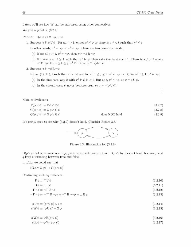
68 CS 720 Class Notes
Later, we’ll see how W can be expressed using other connectives.
We give a proof of (3.2.4).
Proof: ¬(φUψ) ≡ ¬φR¬ψ
1. Suppose π 2 φUψ. For all i ≥ 1, either πi 2 ψ or there is a j < i such that πj 2 φ.
In other words, πi � ¬ψ or πj � ¬φ. There are two cases to consider.
(a) If for all i ≥ 1, πi � ¬ψ, then π � ¬φR¬ψ.
(b) If there is an i ≥ 1 such that πi � ψ, then take the least such i. There is a j > i whereπj � ¬φ. For i ≤ k ≤ j, πk � ¬ψ, so π � ¬φR¬ψ
2. Suppose π � ¬φR¬ψ.
Either (1) ∃i ≥ i such that πi � ¬φ and for all 1 ≤ j ≤ i, πj � ¬ψ; or (2) for all i ≥ 1, πi � ¬ψ.
(a) In the first case, any k with πk � ψ is ≥ i. But at i, πi � ¬φ, so π � φUψ.
(b) In the second case, ψ never becomes true, so π � ¬(φUψ).
More equivalences:
F(φ ∨ ψ) ≡ Fφ ∨ Fψ (3.2.7)G(φ ∧ ψ) ≡ Gφ ∧Gψ (3.2.8)G(φ ∨ ψ) 6= Gφ ∨Gψ does NOT hold (3.2.9)
It’s pretty easy to see why (3.2.9) doesn’t hold. Consider Figure 3.3.
p q
Figure 3.3: Illustration for (3.2.9)
G(p∨ q) holds, because one of p, q is true at each point in time. G p∨G q does not hold, because p andq keep alternating between true and false.
In LTL, we could say that
(Gφ ∨Gψ)→ G(φ ∨ ψ)
Continuing with equivalences:
Fφ ≡ >Uφ (3.2.10)Gφ ≡ ⊥Rφ (3.2.11)
F¬φ ≡ ¬>U¬φ (3.2.12)¬F¬φ ≡ ¬(>U¬φ) ≡ ¬>R¬¬φ ≡ ⊥Rφ (3.2.13)
φUψ ≡ (φWψ) ∧ Fψ (3.2.14)φWψ ≡ (φUψ) ∨Gφ (3.2.15)
φWψ ≡ ψR(φ ∨ ψ) (3.2.16)φRψ ≡ ψW(φ ∧ ψ) (3.2.17)
CS 720 Class Notes 69
A proof of (3.2.16):
Proof: φWψ ≡ ψR(φ ∨ ψ)
1. Suppose π � φWψ.
(a) If there exists an i ≥ 1 such that πi � ψ and for all j ≤ i, πj � φ.
So, for all 1 ≤ j ≤ i, πj � φ ∨ ψ. This is exactly ψR(φ ∨ ψ).
(b) Suppose, for all k ≥ 1, πk � φ. Then for all k ≥ 1, πk � φ ∨ ψ. So, πk � ψR(φ ∨ ψ).
2. Suppose π � ψR(φ ∨ ψ).
(a) Suppose there is an i ≥ 1 where πi � ψ, and πj � φ ∨ ψ for j ≤ i.
Take the least such i; for all j ≤ i, πj � φ, so π � φWψ.
(b) Suppose for all i ≥ 1, πi � φ ∨ ψ.
i. Suppose there is an i ≥ 1. Then πi � ψ. This is like case (2a).
ii. Suppose for all i ≥ 1, πi 2 ψ. So, πi � φ, and π � φWψ
One last equivalence:
φUψ ≡ ¬(¬ψU(¬φ ∧ ¬ψ)) ∧ Fψ (3.2.18)
We can show a derivation for the right side of (3.2.18).
¬(¬ψU(¬φ ∧ ¬ψ)) ∧ Fψ≡(¬¬ψR¬(¬φ ∧ ¬ψ)) ∧ Fψ≡(ψR(φ ∨ ψ)) ∧ Fψ≡φWψ ∨ Fψ≡φUψ
3.2.3 Adequate Connectives for LTL
In linear temporal logic, the following sets of connectives are adequate:
{U,X}{R,X}{W,X}
The connectives F, G can be derived from U, R.
U can derive R. R can derive W.R can derive U. U can derive W.W can derive R. R can derive U.
The set {F,X} is not adequate. F and X are unary connectives; with only unary connectives, we cannotexpress the binary ones.
We cannot define G with {U,F}.We cannot define F with {R,G}.We cannot define F with {W,G}.
An adequate set of connectives for LTL must include X.
70 CS 720 Class Notes
3.2.4 LTL Case Study: The Mutual Exclusion Problem
Huth and Ryan devotes a section to this. We’ll start discussing it now, but read it over for next time.
The Problem: We have a set of concurrent processes that need to access a shared resource. We don’twant multiple processes to access the same shared resource at the same time.
We will introduce critical sections into our code. The shared resource will be accessed from (andonly from) these critical sections. It is not permissible for two processes to be in a critical sectionsimultaneously.
Here are some of the qualities that we desire from our system.
Safety No more than one process in a critical section at any given time.
Liveness If a process wishes to enter a critical section, it will eventually be allowed to do so.
Non-Blocking A process can always request permission to enter a critical section.
No Strict Sequencing Processes need not enter their critical section in strict sequence. For example,if process 1 needs access to its critical section more often than process 2, we shouldn’t impose anordering of {1, 2, 1, 2, 1, 2 . . .} for entry to the critical section.
3.2.5 To-Do
Look into a tool called NuSMV. This is a tool that implements linear temporal logic. It’s introduced inChapter 3.

CS 720 Class Notes 71
3.3 Lecture – 3/26/2007
3.3.1 A Brief Review of LTL Formula Structure
An EBNF for LTL formulas is as follows:
φ ::=>| ⊥| p| (¬φ)| (φ ∧ φ)| (φ ∨ φ)| (φ→ φ)| (Xφ)| (Fφ)| (Gφ)| (φW φ)| (φRφ)| (φUφ)
3.3.2 The Mutual Exclusion Problem
We’ll continue with the mutual exclusion problem that we began looking at during our last lecture. (Seepage 70).
The general idea is as follows: we wish to control access to a resource. We identify a critical section foreach process. Processes may only access the shared resource from within their critical sections. Onlyone process may be in a critical section at any given time.
The qualities we’d like to have:
Safety No more than one process can be in a critical section at any instant in time.
Liveness If a process wishes to enter its critical section, it will eventually be able to do so.
Non-Blocking A process may ask to enter its critical section at any time.
No Strict Sequencing Processes do not have to enter their critical sections in a strict sequence. Wecannot pre-define the order in which processes enter their critical sections.
No Strict Sequencing does not follow from Liveness and Non-Blocking.
Figure 3.7 on Page 181 of Huth & Ryan shows a first attempt at modeling Mutual exclusion. In thisfigure:
• ni – process i is not in its critical section
• ti – process i is trying to enter its critical section
• ci – process i is in its critical section.
Which of our qualities can be modeled using LTL?
Safety Safety can be modeled in LTL.
G(¬(c1 ∧ c2)) (3.3.1)
72 CS 720 Class Notes
Liveness For two processes, we might try to model liveness with the following pair of formulas:
G(t1 → F c1)G(t2 → F c2)
This doesn’t hold for H&R’s figure 3.7. A path that violates these formulas is
s1 → s3 → s7 → s1 → s3 → s7 → . . .
This path shows that it’s possible for t to ask to enter its critical section, but never enters thecritical section.
Non-Blocking For non-blocking, what we really want to say is “for a state where n1 is true, there isa successor where t1 is true”. Unfortunately, LTL does not give us a way to express the existenceof a state. Therefore, Non-Blocking cannot be expressed in LTL.
Another attempt is G(n1 → F t1). This also doesn’t work; it forces process 1 to request entry toits critical section. If process 1 never wishes to enter its critical section, we shouldn’t force it to.
Another attempt that doesn’t work is G(F t1 ∨ ¬F t1). This doesn’t buy us anything because it’sa tautology.
No Strict Sequencing No Strict Sequencing cannot be expressed in LTL, but it’s negation can.
The negation of No Strict Sequencing says the following: all paths that have a c1 period that endscannot have another c1 period until there is a c2 period. (Strict sequence: alternating c1, c2).
In LTL, we can write the negation as
G(c1 → c1 W(¬c1 ∧ ¬c1 W c2))
Figure 3.7 contains a counter example to this formula:
s0 → s5 → s3 → s4 → s5 . . .
Because the negation is false, we conclude that No Strict Sequencing holds.
3.3.3 Computation Tree Logic (CTL)
Computation Tree Logic (CTL) is a branching time logic. It allows quantifiers to be applied to paths.(So, you can say “there exists a path”).
CS 720 Class Notes 73
EBNF for CTL
An EBNF for CTL appears below:
φ ::=⊥| >| p| (¬φ)| (φ ∧ φ)| (φ ∨ φ)| (φ→ φ)| (AXφ)| (EXφ)| (AFφ)| (EFφ)| (AGφ)| (EGφ)| (A[φUφ])| (E[φUφ])
Binding order for CTL Operators and Quantifiers
The precedence order for CTL is as follows:
¬,AG,EG,AF,EF,AX,EX∧,∨→,A[U],E[U]
Before we get further into definitions, let’s look at a some examples to get an intuitive feel for how CTLworks.
Example 3.3.1: EF q. There is reachable state satisfying q.
Example 3.3.2: AG(p → E[pU q]). From all reachable states satisfying p, it is possible to maintain puntil we reach a state satisfying q.
Example 3.3.3: AG(p→ EG q). Whenever a state satisfying p is reached, there is a path where q willbe true forevermore.
Example 3.3.4: EF AG p. There is a reachable state from which all reachable states satisfy p.
The quantifiers U, F, G, and X retain their meaning from LTL.
The quantifiers A and E mean “for all paths”, and “for some path”, respectively.
3.3.4 Semantics of CTL
Definition 3.3.5 (Transition System): A transition system M = (S,→, L) is a set of states S, endowedwith a transition relation →, and a labeling function L : S → P(atoms)

74 CS 720 Class Notes
This is the same definition we saw with LTL. There are nodes, edges, and truth values (labels) assignedto nodes.
CTL formulas are also interpreted over transition systems.
Let M = (S,→, L) be a model, let s be a state s ∈ S, and let φ be a CTL formula. Whether M, s � φcan be understood as follows:
1. If φ is atomic, satisfaction is determined by L.
2. If the top-level connective of φ is a boolean connective (∧, ∨, →, etc), then the answer comes from(1) the usual truth-table style of evaluation applied to the operator and (2) recursively evaluatingeach of the operands.
3. If the top connective is an operator beginning with ‘A’, then satisfaction holds if all paths satisfythe ‘LTL Formula’ resulting from removing the leading A symbol.
4. If the top-level connective begins with ‘E’, then satisfaction holds if some path from s satisfies the‘LTL Formula’ that results from removing the leading E.
These rules are a little loose – removing a leading A or E does not necessarily produce a formula that isstrictly LTL.
CTL Semantics, more formally
1. M, s � > and M, s 2 ⊥
2. M, s � p IFF p ∈ L(s)
3. M, s � ¬φ IFF M, s 2 φ
4. M, s � φ1 ∧ φ2 IFF M, s � φ1 and M, s � φ2.
5. M, s � φ1 ∨ φ2 IFF M, s � φ1 or M, s � φ2.
6. M, s � φ1 → φ2 IFF M, s 2 φ1 or M, s � φ2.
7. M, s � AXφ IFF for all s1 such that s→ s1 we have M, s1 � φ. AX says “In every next state”
8. M, s � EXφ IFF for some s1 such that s→ s1 we haveM, s1 � φ. EX says “In some next state”.EX and AX are duals.
9. M, s � AGφ holds IFF for all paths s1 → s2 → s3 . . . where s1 equals s and si along the path, wehave Msi � φ.
For all paths beginning with s, φ holds globally. This includes s itself.
10. M, s � EGφ holds IFF there is a path paths s1 → s2 → s3 . . . where s1 equals s and si along thepath, we have Msi � φ.
There exists a path beginning with s such that φ holds globally along that path.
11. M, s � AFφ holds IFF for all paths s1 → . . ., there is some si such that M, si � φ.
For all computation paths beginning with s, there will be some future state where φ holds.
12. M, s � EFφ holds IFF for some path M, si � φ.
There exists a computation path beginning with s, such that φ holds in some future state.
13. M, s � A[φ1 Uφ2] holds IFF for all paths, that path satisfies [φ1 Uφ2].
There is some si along the path such that M, si � φ2 holds, and for all 1 ≤ j < i, we haveM, sj � φ1.
All computation paths beginning with s satisfy φ1 until φ2 becomes true.
CS 720 Class Notes 75
14. M, s � E[φ1 Uφ2] holds IFF there is some path that satisfies [φ1 Uφ2].
There exists a computation path beginning with s such that φ1 holds until φ2 holds.
More Examples
Example 3.3.6: EF(started ∧ ¬ready). You can reach a state where started is true and ready is false.
Example 3.3.7: AG(requested→ AF acknowledged).
For all states (globally), if requested is true, then for every path acknowledged will become true at somepoint. This is a good property for a service protocol.
Example 3.3.8: AG AF enabled → AG AF running. On every path, if enabled is true infinitely often,then on every path, running will be true infinitely often. The left side of the implication is strong, whichmakes it a weak assertion (easy for the LHS to be false).
Contrast this with the LTL formula G F enabled→ G F running. This means, on every path, if enabled istrue infinitely often, then running is true infinitely often.
The LTL version is more particular; it is also inexpressible in CTL.
Example 3.3.9: AF AGφ. On every path, you’ll reach a point where φ is globally true.
Example 3.3.10: AG EFφ. From every path, you can reach a state where φ will become true in thefuture.
Example 3.3.11 (Non-Blocking in CTL): In CTL we can express our non-blocking property as AG(n1 →EX t1).
3.3.5 LTL vs CTL
Implicitly, there is an A quantifier in every LTL formula. LTL requires the formula to be true on everypath.
Not all LTL formulas can be expressed in CTL.
Not all CTL formulas can be expressed in LTL.
Sometimes one can turn an LTL formula into a CTL formula by adding the A quantifier.

76 CS 720 Class Notes
3.4 Lecture – 3/28/2007
3.4.1 Mutual Exclusion in CTL and LTL
We’ll finish our analysis of mutual exclusion with a comparison of how CTL and LTL handle the problem.
SafetyIn LTL: G¬(c1 ∧ c2)In CTL: AG¬(c1 ∧ c2)
LivenessIn LTL: G(n1 → F c1)In CTL: AG(n1 → AF c1)
Non-BlockingIn LTL: Not expressibleIn CTL: AG(n1 → EX t1)
No Strict SequencingIn LTL: We could express the negation, G(c1 → c1 W(¬c1 ∧ ¬c1 W c2))In CTL: EF(c1 ∧ E[c1 U(¬c1 ∧ E[¬c2 U c1])])
Figure 3.4 gives a visual representation of the CTL formula for no strict sequencing.
¬1 c1 c1
c2 c2c2¬ ¬ ¬
c
Figure 3.4: Visual representation of No Strict Sequencing under CTL
3.4.2 CTL Equivalences
Some of CTL’s equivalences are like standard quantifier negation.
¬AFφ ≡ EG¬φ¬EFφ ≡ AG¬φ¬AXφ ≡ EX¬φ¬EXφ ≡ AX¬φ
AFφ ≡ A[>Uφ]EFφ ≡ E[>Uφ]
AXφ ≡ ¬EX¬φAGφ ≡ ¬EF¬φEGφ ≡ ¬AF¬φ

CS 720 Class Notes 77
3.4.3 Adequate Connectives in CTL
Theorem 3.4.1: A set of CTL connectives is adequate IFF it contains
• one of {AX,EX}• one of {EG,AF,A U}• and E U
Example 3.4.2: The set of connectives {EX,A U,E U} is adequate for CTL. From the equivalencesgiven earlier, it’s not difficult to see how the 8 CTL connectives can be derived.
Example 3.4.3: The set of connectives {EX,EG,E U} is adequate. This set is like the one appearingin Example 3.4.2. The only differences is EG instead of A U – we just need to show that A U can beexpressed using the connectives we have.
We have the equivalence
A[φUψ] ≡ A[¬(¬ψU(¬φ ∧ ¬ψ)) ∧ Fψ]
This isn’t strictly a CTL formula, but it is a CTL* formula. We can manipulate this as follows:
≡ ¬E¬[¬(¬ψU(¬φ ∧ ¬ψ)) ∧ Fψ]≡ ¬E[¬ψU(¬φ ∧ ¬ψ) ∨ ¬Fψ]≡ ¬E(¬ψU(¬φ ∧ ¬ψ)) ∨ E[¬Fψ]≡ ¬E(¬ψU(¬φ ∧ ¬ψ)) ∨ E G¬ψ
From the last line, we have expressed A U with EG.
Example 3.4.4: The connectives {EX,AF E U} are another adequate set.
3.4.4 What’s Not A Connective in CTL
CTL doesn’t adopt all of LTL’s connectives. For example there’s no AR, ER, AW, or EW.
This doesn’t limit the expressiveness of CTL. In LTL, we saw that R and W could be derived. The samething could be done in CTL.
A[φRψ] ≡ A[¬(¬φU¬ψ)]≡ ¬E[¬φU¬ψ]
E[φRψ] ≡ ¬A[¬φU¬ψ]A[φWψ] ≡ A[ψR(φ ∨ ψ)]E[φWψ] ≡ E[ψR(φ ∨ ψ)]
3.4.5 More CTL Equivalences
The equivalences that follow are recursive. Instead of simply making an assertion from the current state,they say something about the current state and the state that follows. Studying them gives a good idea
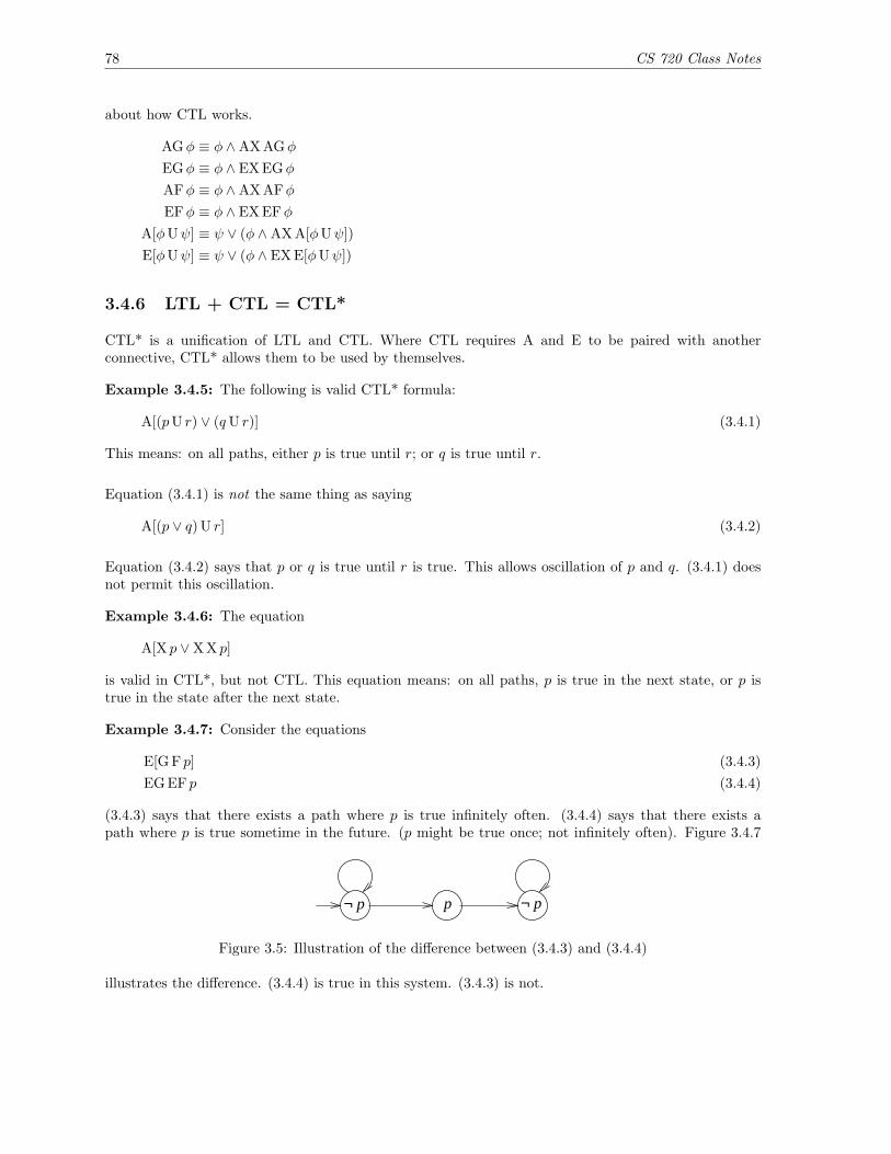
78 CS 720 Class Notes
about how CTL works.
AGφ ≡ φ ∧AX AGφ
EGφ ≡ φ ∧ EX EGφ
AFφ ≡ φ ∧AX AFφEFφ ≡ φ ∧ EX EFφ
A[φUψ] ≡ ψ ∨ (φ ∧AX A[φUψ])E[φUψ] ≡ ψ ∨ (φ ∧ EX E[φUψ])
3.4.6 LTL + CTL = CTL*
CTL* is a unification of LTL and CTL. Where CTL requires A and E to be paired with anotherconnective, CTL* allows them to be used by themselves.
Example 3.4.5: The following is valid CTL* formula:
A[(pU r) ∨ (qU r)] (3.4.1)
This means: on all paths, either p is true until r; or q is true until r.
Equation (3.4.1) is not the same thing as saying
A[(p ∨ q) U r] (3.4.2)
Equation (3.4.2) says that p or q is true until r is true. This allows oscillation of p and q. (3.4.1) doesnot permit this oscillation.
Example 3.4.6: The equation
A[X p ∨X X p]
is valid in CTL*, but not CTL. This equation means: on all paths, p is true in the next state, or p istrue in the state after the next state.
Example 3.4.7: Consider the equations
E[G F p] (3.4.3)EG EF p (3.4.4)
(3.4.3) says that there exists a path where p is true infinitely often. (3.4.4) says that there exists apath where p is true sometime in the future. (p might be true once; not infinitely often). Figure 3.4.7
pp ¬ p¬
Figure 3.5: Illustration of the difference between (3.4.3) and (3.4.4)
illustrates the difference. (3.4.4) is true in this system. (3.4.3) is not.
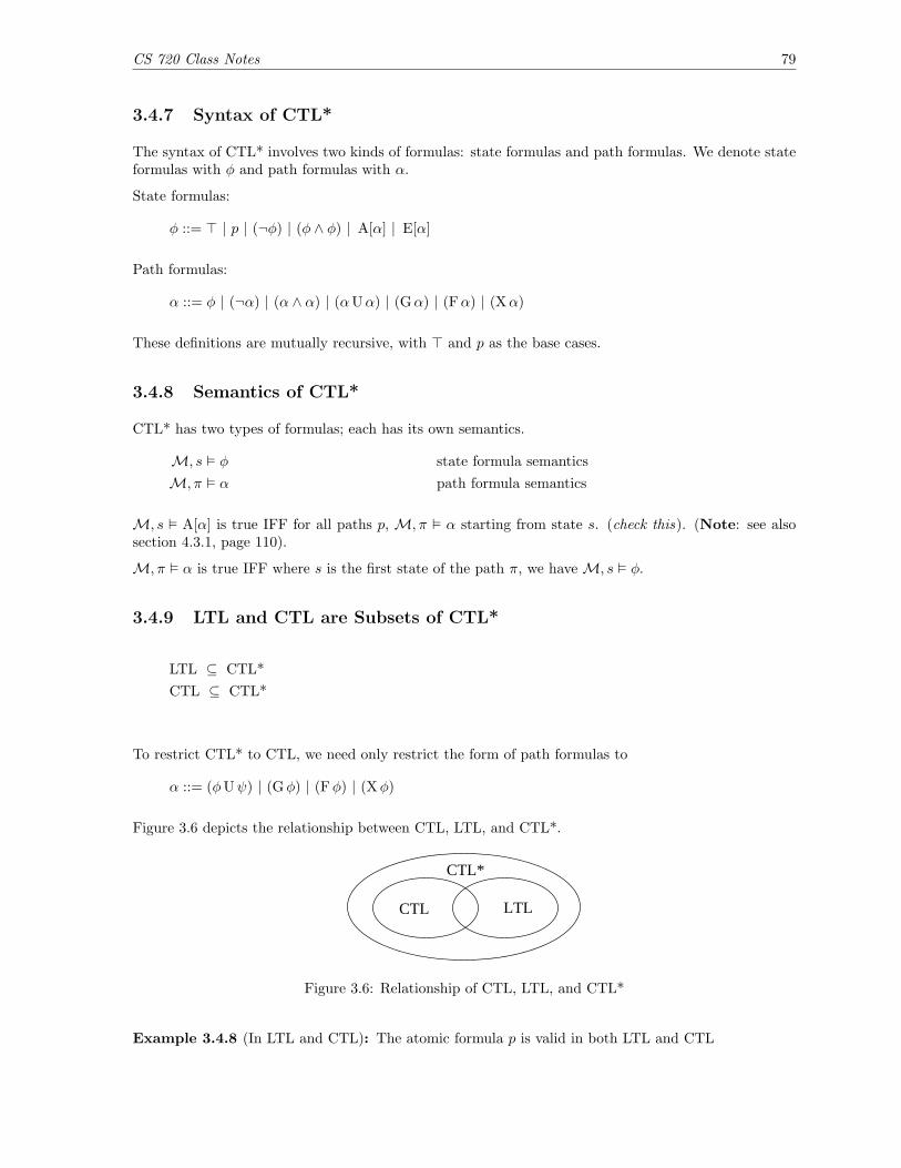
CS 720 Class Notes 79
3.4.7 Syntax of CTL*
The syntax of CTL* involves two kinds of formulas: state formulas and path formulas. We denote stateformulas with φ and path formulas with α.
State formulas:
φ ::= > | p | (¬φ) | (φ ∧ φ) | A[α] | E[α]
Path formulas:
α ::= φ | (¬α) | (α ∧ α) | (αUα) | (Gα) | (Fα) | (Xα)
These definitions are mutually recursive, with > and p as the base cases.
3.4.8 Semantics of CTL*
CTL* has two types of formulas; each has its own semantics.
M, s � φ state formula semanticsM, π � α path formula semantics
M, s � A[α] is true IFF for all paths p, M, π � α starting from state s. (check this). (Note: see alsosection 4.3.1, page 110).
M, π � α is true IFF where s is the first state of the path π, we have M, s � φ.
3.4.9 LTL and CTL are Subsets of CTL*
LTL ⊆ CTL*CTL ⊆ CTL*
To restrict CTL* to CTL, we need only restrict the form of path formulas to
α ::= (φUψ) | (Gφ) | (Fφ) | (Xφ)
Figure 3.6 depicts the relationship between CTL, LTL, and CTL*.
CTL*
CTL LTL
Figure 3.6: Relationship of CTL, LTL, and CTL*
Example 3.4.8 (In LTL and CTL): The atomic formula p is valid in both LTL and CTL

80 CS 720 Class Notes
Example 3.4.9 (CTL, Not LTL): The formula AG EF p can be expressed in CTL, but cannot beexpressed in LTL. (We’ll see why shortly, when we examine the sub-model property).
Example 3.4.10 (LTL, Not CTL): The formula A[G F p→ F q] can be expressed in LTL, but not CTL.
Example 3.4.11 (CTL* only): The formula E[G F p] cannot be expressed in LTL, and it cannot beexpressed in CTL. It’s only expressible in CTL*.
3.4.10 The Sub-model Property of LTL
Definition 3.4.12 (submodel): LetM = (S,→, L) be a model. M′ = (S′,→′, L′) is a sub-model ofMif
S′ ⊆ S→′ ⊆→L′ = L � S′
L � S′ means “L restricted to S′”.
Theorem 3.4.13 (Submodel Property): If A[α] is an LTL formula, and M′ is a sub-model of M, ands ∈ S′, then
M, s � A[α]→M′, s � A[α]
If an LTL formula φ is valid for a model M, then φ is also valid for any sub-model M′ of M.
Theorem 3.4.13 gives us a way to prove that a given φ is not LTL. If you can find a model M where φholds, and a sub-model M′ where φ does not hold, then φ is not an LTL formula.
Example 3.4.14: Consider the M and M′ shown in Figure 3.7.
M p
¬ pM’
p¬
Figure 3.7: Model M and sub-model M′
The formula φ = AG EF p holds for M. At any point, there is a future state where p is true.
AG EF p does not hold for M′ (p is never true). Because φ does not hold for M′, φ is not an LTLformula.

CS 720 Class Notes 81
3.5 Lecture – 4/2/2007
3.5.1 CTL vs CTL*
There are two differences between CTL and CTL*:
1. CTL does not allow the boolean combination of path formulas. For example, you can’t sayE[(pU q) ∧ (pR r)].
2. CTL does not allow one path operator to be applied to another path operator. For example, youcan’t say G F p.
Difference (1) can be gotten around. Boolean combinations of path formulas can usually be expressedusing CTL equivalences.
Example 3.5.1: Using equivalences to achieve the effect of boolean combinations of path formulas inCTL.
E[F p ∨ F q] ≡ EF p ∨ EF qE[F p ∧ F q] ≡ E[F(p ∧ EF q)] ∨ E[F(q ∧ EF p)]A[F p ∨ F q] ≡ AF(p ∨ q)A[G p ∨G q] ≡?
Difference (2) we’re stuck with. There’s no way to work around it in CTL.
3.5.2 Past Connectives
The path operators we’ve seen refer to future states. We could consider augmenting them with operatorsthat refer to path states. For example
Y Yesterday Past version of XS Since Past version of UO Once Past version of XH Historically Past version of G
Example 3.5.2 (Past Connectives):
G(p→ Op)
Globally, if q is true then p is true now, or p was true at some point in the past. This is equivalent tothe formulas
¬pW q
¬(¬qU(p ∧ ¬q))
Past operators do not add any expressive power to LTL. LTL considers single paths. Past operatorsallow us to travel backward along that path, but only to points reachable by traveling forward from thestart state.
Past operators do add expressive power to CTL. CTL gives us no way to say things about states thatare not forward reachable.
82 CS 720 Class Notes
3.5.3 Model Checking
The general question for temporal logic checking is as follows: does the initial state of a transition systemsatisfy the given LTL or CTL formula? Or, does M, s0 � φ for the starting state s0.
Usually it’s easier to find a list of states that satisfy φ. If the starting state satisfies φ, then M, s � φholds. In other words, find states
{s ∈ S | M, s � φ}
3.5.4 CTL Labeling Algorithms
We first rewrite φ as follows:
• Use only the propositional connectives ⊥, ∧, and ¬.• Use only the CTL connectives AF, E U, EX. Limiting ourselves to a single adequate set of CTL
connectives simplifies the algorithm.
Next, we label each model state with all sub-formulas that are satisfied at that state. This is an iterativeprocess.
• ⊥. No state is labeled with ⊥
• p. Label s with p if p ∈ L(s).
• ψ1 ∧ ψ2. If s is labeled with both ψ1 and ψ2, then label s with ψ1 ∧ ψ2.
• AFψ.
– If any state s is labeled with ψ, then label s with AFψ.– Repeat until no change: Label any state s′ with AFψ if all successors of s′ are labeled with
AFψ.
• E[ψ1 Uψ2].
– If any state s is labeled with ψ2, label s with E[ψ1 Uψ2].– Repeat until no change: label s′ with E[ψ1 Uψ2] if s′ is labeled with ψ1 and at least one
successor of s′ is labeled with E[ψ1 Uψ2].
• EXψ. Label s with EXψ if at least one successor of s is labeled with ψ.
3.5.5 CTL Satisfiability Algorithm
Below, φ is assumed to be a well-formed CTL formula.
procedure SAT(φ)if φ is > then
return S . S = all stateselse if φ is ⊥ then
return ∅else if φ is atomic then
return {s ∈ S | φ ∈ L(s)}else if φ is ¬φ1 then
return S − SAT(φ1)else if φ is φ1 ∧ φ2 then
return SAT(φ1) ∩ SAT(φ2)else if φ is φ1 ∨ φ2 then
return SAT(φ1) ∪ SAT(φ2)

CS 720 Class Notes 83
else if φ is φ1 → φ2 thenreturn SAT(¬φ1 ∨ φ2)
else if φ is AXφ1 thenreturn SAT(¬EX¬φ1)
else if φ is EXφ1 thenreturn SATEX(φ1)
else if φ is A[φ1 Uφ2] thenreturn SAT(¬(E[¬φ2 U(¬φ1 ∧ ¬φ2)] ∨ EG¬φ2))
else if φ is E[φ1 Uφ2] thenreturn SATEU(φ1, φ2)
else if φ is EFφ1 thenreturn SAT(E[>Uφ1])
else if φ is EGφ1 thenreturn SAT(¬AF¬φ1)
else if φ is AFφ1 thenreturn SATAF(φ1)
else if φ is AGφ1 thenreturn SAT(¬EF¬φ1)
end ifend procedure
The function SATEX, SATEU, SATAF are helpers. These are detailed later.
The helpers rely on these two auxiliary functions:
pre∃(Y ) = {s ∈ S | exists s′, (s→ s′ and s′ ∈ Y )} (3.5.1)pre∀(Y ) = {s ∈ S | for all s′, (s→ s′ implies s′ ∈ Y )} (3.5.2)
Both (3.5.1) and (3.5.2) compute pre-images of states.
pre∃ returns a set of states that can make a transition into Y .
pre∀ returns a set of states that only make transitions into Y .
In an ideal world, we’d want SAT to have a running time that is proportional to (a) the size of the formulaand (b) the size of the model. In other words, Θ(|φ| · (|V |+ |E|))
Procedure SATAF
The function SATAF works as described in Section 3.5.4 on Page 82.
procedure SATAF(φ)X = S . S is the set of all model statesY = SAT(φ)repeat
X = YY = Y ∪ pre∀(Y )
until X = Y . Until no changereturn Y
end procedure
The disadvantage with SATAF is its running time: proportional to Θ(V · (V +E)). Later, we’ll look at abetter algorithm.
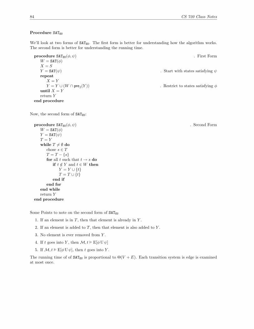
84 CS 720 Class Notes
Procedure SATEU
We’ll look at two forms of SATEU. The first form is better for understanding how the algorithm works.The second form is better for understanding the running time.
procedure SATEU(φ, ψ) . First FormW = SAT(φ)X = SY = SAT(ψ) . Start with states satisfying ψrepeat
X = YY = Y ∪ (W ∩ pre∃(Y )) . Restrict to states satisfying φ
until X = Yreturn Y
end procedure
Now, the second form of SATEU:
procedure SATEU(φ, ψ) . Second FormW = SAT(φ)Y = SAT(ψ)T = Ywhile T 6= ∅ do
chose s ∈ TT = T − {s}for all t such that t→ s do
if t /∈ Y and t ∈W thenY = Y ∪ {t}T = T ∪ {t}
end ifend for
end whilereturn Y
end procedure
Some Points to note on the second form of SATEU
1. If an element is in T , then that element is already in Y .
2. If an element is added to T , then that element is also added to Y .
3. No element is ever removed from Y .
4. If t goes into Y , then M, t � E[φUψ]
5. If M, t � E[φUψ], then t goes into Y .
The running time of of SATEU is proportional to Θ(V + E). Each transition system is edge is examinedat most once.

CS 720 Class Notes 85
Procedure SATEX
The procedure to determine satisfaction of EXφ is pretty straightforward:
procedure SATEX(φ)X = SAT(φ)Y = pre∃(X)return Y
end procedure
3.5.6 A more efficient way to handle EGψ
There is a more efficient algorithm to handle EGψ.
• Label all states with EGψ.
• If any state is not labeled with ψ, then delete EGψ.
• Repeat until no change: delete EGψ from s if no successor of s is labeled with EGψ.
This algorithm is given a more thorough treatment on page 86.

86 CS 720 Class Notes
3.6 Lecture – 4/4/2007
3.6.1 CTL Model Checking
We’ve looked at three helper functions for checking CTL models. These functions, and their runningtimes are
• SATAF– Θ(|φ| · |V | · (|V |+ |E|))• SATEU– Θ(|φ| · (|V |+ |E|))• SATEX– Θ(|φ| · (|V |+ |E|))
These Θ values are slightly misleading. We’re talking about transition systems; every node must have atleast one outgoing edge. Therefore, the number of edges will be ≥ the number of nodes. |E| dominates|V | in the complexity values above.
3.6.2 SATEG: A Better Version of SATAF
The equivalence EGφ ≡ ¬AF¬φ allows us to write a more efficient SATAF, one whose running time is alinear function of the model size.
We’ll call this function SATEG.
Definition 3.6.1 (Strongly Connected Component): A strongly connected component (SCC) in a di-rected graph is a maximal subset such that each vertex is connected to each other component vertex bya path.
Example 3.6.2: Figure 3.8 shows a directed graph with two strongly connected components. Onecomponent consists of vertices {a, b, c}. The second component consists of the vertex {d}.
d
a b
c
Figure 3.8: Two Strongly Connected Components
A single vertex is always strongly connected (it has a path of length zero to itself).
Definition 3.6.3 (Non-Trivial SCC): A Strongly connected component is non-trivial if (a) it containsmore than one node or (b) it contains one node with a loop to itself (like d in Figure 3.8).
Let M′ be obtained by M by deleting states where φ is false. M′ may not be a transition system, butit will still be a directed graph.
Claim 3.6.4: M, s � EGφ IFF
1. s ∈ S′. φ must be true in state s.2. There is a path in M′ from s to a non-trivial strongly connected component of M′.
Proof: Case 1 (if):
• Let π be a path starting at s, with φ true everywhere on π.

CS 720 Class Notes 87
• π is a path of M′, because M′ consists only of states where φ is true.
• Let us divide π into two paths: π0 (a finite path) and π1 (an infinite path). In π1 every state willoccur infinitely often.
• Every state in π1 is connected to every other state in π1.
• ∴ states in π1 are contained in a strongly connected component of M′.
Case 2 (only if):
• Suppose s ∈ S′, and suppose that there is a path inM′ from s to a strongly connected componentof M′
• This gives an infinite path from s with φ true everywhere along that path.
There is a linear-time algorithm to compute strongly connected components. The algorithm is due toTarjen; the CLR algorithms book should have it.
procedure SATEG(φ)W = SAT(φ)Y =
⋃{c | c is an SCC of W}
T = Ywhile T 6= ∅ do
chose s ∈ TT = T − {s}for all t such that t→ s do
if t /∈ Y and t ∈W thenY = Y ∪ {t}T = T ∪ {t}
end ifend for
end whilereturn Y
end procedure
Because SATEG is a linear-time algorithm, the entire SAT procedure has running time linear in the size ofthe model.
3.6.3 The State Explosion Problem
SAT is linear in the size of the model. Unfortunately, the size of the model can grow at a non-linear ratewith respect to the formula. For example, adding one variable could double the number of model states.Although the algorithm is linear, the size of the problem is not.
To effectively deal with large models, we’d really like more than just a linear-time algorithm.
There are techniques that address the state explosion problem. One of these is called an OBDD , orordered binary decision tree. An OBDD is a data structure. We’ll look at them later in the semester.
3.6.4 CTL Model Checking With Fairness
Consider a fragment from our mutual exclusion problem:

88 CS 720 Class Notes
1 n1t2 c2c
Figure 3.9: A Fragment of the Mutual Exclusion Problem
Figure 3.9 shows two states: (a) process 1 in a critical section; process 2 waiting to enter a critical sectionand (b) process one outside the critical section, process two in the critical section.
Our model assumes that all state transitions happen in a single clock tick. But what if process 1 neededto stay in its critical section for longer than one tick? We’d have to add another edge, like the one inFigure 3.10
1 n1t2 c2c
Figure 3.10: Allowing process 1 to stay in its critical section
The new edge in Figure 3.10 creates a problem: process one may stay in its critical section indefinitely,violating liveness. Process two has asked to enter its critical section – when will it be able to do so?
We can augment CTL with fairness constraints. The model checker must consider only those pathswhich satisfy fairness constraints infinitely often.
Example 3.6.5: Fairness constraints for mutual exclusion:
G F¬c1 Process 1 must leave its critical section infinitely oftenG F¬c2 Likewise for process 2
Definition 3.6.6 (Fairness): Let C = {ψ1, . . . , ψn} be a set of fairness constraints. (They’ll actuallybe CTL formulas). A path π = s1 → s2 → . . . is fair with respect to C if, for all i there are infinitelymany j such that
M, sj � ψi
Every fairness constraint must occur infinitely often.
We can augment the CTL quantifiers:
AC Every path is fairEC There exists a fair path
AC and EC are like A and E, but they’re restricted to fair paths.
Some equivalences for fair quantifiers:
EC[φUψ] ≡ E[φU(ψ ∧ ECG>)]ECXφ ≡ EX(φ ∧ ECG>)
Claim 3.6.7: A computation path is fair IFF any suffix of the path is fair.
Given these equivalences, we need only supply an algorithm for ECG.
CS 720 Class Notes 89
Algorithm for ECG
The algorithm for ECG is similar to SATEG.
• Restrict the graph to states satisfying φ. Call this M′. Of M′, we want to know which statescomprise fair paths.
• Find the maximal strongly connected components of M′.
• Remove an SCC if, for some fairness constraint ψi the SCC does not contain a state satisfying ψi.The resulting SCCs are the fair SCCs.
• Use backwards breadth-first search to find the states of M′ that can reach a fair SCC.
Definition 3.6.8 (Fair SCC): A strongly connected component of M′ is fair if for all 1 ≤ i ≤ n, theSCC contains a state in SAT(ψi). (Where each ψi is a fairness constraint, expressed as a CTL formula).
The running time of our ECG algorithm is Θ(|C| · (|V |+ |E|)).
3.6.5 Fairness Constraints in LTL
Fairness constraints require no special handling in LTL. We express the constraints as LTL formulas andinsist that they occur infinitely often. Like this:
(G Fψ1 ∧G Fψ2 ∧ . . . ∧G Fψn)→ φ (3.6.1)
Translation: if the fairness constraints ψi are met, then φ has to be true.
3.6.6 LTL Model Checking
There are algorithms for model checking LTL formulas, but they tend to be more complicated thanCTL. LTL model checkers tend to be based on (a) tableaux or (b) Buchi automata.
Buchi automata are specialized automata, able to handle strings of infinite length. Why the issue ofinfinite-length strings? A path through a model can be infinitely long. In the context of an automata,when can you accept a string of infinite length?
90 CS 720 Class Notes
3.7 Lecture – 4/9/2007
3.7.1 LTL Model Checking
It’s sufficient to give an algorithm that checks whether M, s � Eφ.
Note thatM, s � Aφ IFFM, s 2 E¬φ. (According to H&R, given φ, we’ll checkM, s � E¬φ. If φ holdsfor all paths, ¬φ won’t hold for any. But, if ¬φ holds for some path, then we’ll have a counterexample).
We’ll assume that φ uses only the following connectives >, ¬, ∨, X, and U.
Definition 3.7.1 (Closure): The closure of φ, written C(φ) is the set of all positive sub-formulas of φand their negations.
Example 3.7.2: Given φ = pU q ∨ ¬pU r
C(pU q ∨ ¬pU r) = {p, q, r, pU q,¬pU r,¬p,¬q,¬r,¬(pU q),¬(¬pU r)}
Definition 3.7.3 (automaton): We define an automaton Aφ as an automaton for φ (really a directedgraph). Aφ accepts traces of propositional atoms such that φ is true along the path of the trace.
Aφ = (T, δ)
where δ is a transition relation and T is the set of all (consistent) subsets q of C(φ).
Formulas in T must be locally consistent.
• For all positive sub-formulas ψ ∈ C(φ), either ψ ∈ q or ¬ψ ∈ q, but not both.
• For all ψ1 ∨ ψ2 ∈ C(φ), ψ1 ∨ ψ2 ∈ q IFF ψ1 ∈ q or ψ2 ∈ q.
• For all ψ1 Uψ2 ∈ C(φ), ψ1 Uψ2 ∈ q IFF ψ2 ∈ q or ψ1 ∈ q.
• For all ¬(ψ1 Uψ2) ∈ C(φ), if ¬(ψ1 Uψ2) ∈ q, then “¬ψ2 ∈ q”. More precisely, if ψ2 is positive,then ¬ψ2 ∈ q.
On the other hand, if ψ2 = ¬ψ′2, then ψ′2 ∈ q.
We’ll also need a transition function, δ, where (q, q′) ∈ δ.
• If Xψ ∈ q, then ψ ∈ q′.
• if ¬Xψ ∈ q, then ¬ψ ∈ q′. (This assumes that ψ is positive).
• If ¬X¬ψ ∈ q then ψ ∈ q′.
• If ψ1 Uψ2 ∈ q and ψ2 /∈ q, then ψ1 Uψ2 ∈ q′.
Note that this has the effect of “pushing” ψ1 Uψ2 along the path.
• Suppose ¬(ψ1 Uψ2) ∈ q and ψ1 ∈ q. Then ¬(ψ1 Uψ2) ∈ q′.
These rules describe the transition system Aφ = (T, δ). This is an abstract system. It doesn’t describeany particular model M.
Our next step is to attach a model to the abstract automata, forming M×Aφ.
M×Aφ = (U, δ′)
where
U = {(s, q) ∈ S × T | for all atoms p ∈ C(φ), p ∈ q IFF p ∈ L(s)}δ′ = {(s, q), (s′, q′) | s→ s′ ∈M and q → q′ ∈ δ}
CS 720 Class Notes 91
Given M×Aφ, is φ true from a given state s?
Definition 3.7.4 (Eventuality Sequence): An eventuality sequence is a path (s0, q0), (s1, q1) ∈M×Aφsuch that if ψ1 Uψ2 ∈ qi for some i, then ψ2 ∈ qj for some j ≥ i.
(It seems like an eventuality sequence is a path, where ‘until’ holds along that path).
Theorem 3.7.5: M, s � Eφ IFF there is an eventuality sequence inM×Aφ starting with (s, q) whereφ ∈ p.
The proof of theorem 3.7.5 is pretty long. We’ll take it in pieces.
Claim 3.7.6: For all ψ ∈ C(φ) and for all i ≥ 0, πi � ψ IFF ψ ∈ qi.
Proof: The proof is by induction on ψ. There are five cases to consider.
1. If ψ = p (an atom), then πi � p IFF p ∈ L(si). This happens IFF p ∈ qi.
2. ψ = ¬ψ1 (Left as an exercise for the reader).
3. ψ = ψ1 ∨ ψ2 (left as an exercise for the reader).
4. ψ = Xψ1. (assume ψ1 positive)
Suppose πi satisfies ψ. Then πi+1 � ψ1.
πi+1 � ψ1 IFF ψ1 ∈ qi+1 and IFF ψ ∈ qi.
If Xψ1 ∈ qi, then ψ1 ∈ qi+1.
If Xψ1 /∈ qi, then ¬Xψ1 ∈ qi and ¬ψ1 ∈ qi+1 and ψ1 /∈ qi+1.
5. ψ = ψ1 Uψ2. (assume ψ2 positive). There are two cases to consider.
(a) Suppose πi = ψ. Then there is a j ≥ i such that πj � ψ2 and for all 1 ≤ i ≤ j, πi � ψ1.
By the inductive hypothesis, if πj � ψ2, then ψ2 ∈ qj , and for all 1 ≤ i ≤ j, π1 ∈ qi.
Let us choose a minimal j. For i < j, we have ¬ψ2 (because j was chosen to be minimal).
ψ1 Uψj ∈ qj , because ψ2 ∈ qj . (If this were not the case, we’d have ¬(ψ1 Uψ2) ∈ qj , and¬ψ2 ∈ qj – a contradiction).
Suppose ¬(ψ1 Uψ2) ∈ qi and ψ1 ∈ qi. By the transition system rules, we’d have ¬(ψ1 Uψ2) ∈qi+1 and ψi ∈ qi+1. This would mean that ¬(ψ1 Uψ2) ∈ qj – another contradiction.
∴ (ψ1 Uψ2) ∈ qi.
(b) Suppose ψ = ψ1 Uψ2 ∈ qi. We must show that πi � ψ.
By definition of eventuality sequence, there exists a j ≤ i such that ψ2 ∈ qj .
Take j to be minimal. We show by induction on k that for 1 ≤ i ≤ k ≤ j, that ψ1 Uψ2 ∈ qk.
The Basis case is given: ψ1 Uψ2 ∈ qi.
Inductive Case: Suppose i ≤ k < j, and ψ1 Uψ2 ∈ qk. By our definition of j (minimal),ψ2 /∈ qk. So, ¬ψ2 ∈ qk, and ψ1 Uψ2 ∈ qk+1.
For i ≤ k < j, we have ψ1 Uψ2 ∈ qk. But we also know that ψ2 /∈ qk (j was chosen to beminimal). So ψ1 ∈ qk.
By the inductive hypothesis, for 1 ≤ k < j, πk � ψ1 and πj � ψ2, so πi � ψ1 Uψ2 = ψ.

92 CS 720 Class Notes
See Section 3.9.2 (page 94) for the second half of the proof.
CS 720 Class Notes 93
3.8 H&R Notes on LTL Model Checking – 4/11/2007
3.8.1 States of Aφ
The states of Aφ (denoted as q are the maximal subsets of C(φ) that satisfy the following conditions:
• For all (non-negated) ψ ∈ C(φ), either ψ ∈ q or ¬ψ ∈ q, but not both.
• ψ1 ∨ ψ2 ∈ q holds IFF ψ1 ∈ q or ψ2 ∈ q whenever ψ1 ∨ ψ2 ∈ C(φ).
• Conditions for other boolean combinations are similar.
• If ψ1 Uψ2 ∈ q, then ψ2 ∈ q or ψ1 ∈ q.
• If ¬(ψ1 Uψ2) ∈ q, then ¬ψ2 ∈ q.
Intuitively, these conditions imply that the state of Aφ are capable of saying which sub-formulas of φare true.
The initial states of Aφ are those states containing φ.
3.8.2 Transitions of Aφ
δ is the transition relation of Aφ. Two states (q, q′) ∈ δ IFF all of the following conditions hold:
• If Xψ ∈ q, then ψ ∈ q′
• If ¬Xψ ∈ q, then ¬ψ ∈ q′
• If ψ1 Uψ2 ∈ q and ψ2 /∈ q, then ψ1 Uψ2 ∈ q′. (Note: this has the effect of “pushing” the untilalong the path).
• If ¬(ψ1 Uψ2) ∈ q and ψ1 ∈ q, then ¬(ψ1 Uψ2) ∈ q′. (Again, pushing the until).
These rules are based on the recursion laws:
ψ1 Uψ2 ≡ ψ2 ∨ (ψ1 ∧X(ψ1 Uψ2)) (3.8.1)¬(ψ1 Uψ2) ≡ ¬ψ2 ∧ (¬ψ1 ∨X¬(ψ1 Uψ2)) (3.8.2)
94 CS 720 Class Notes
3.9 Lecture – 4/11/2007
3.9.1 LTL Model Checking
Last class, we began to look at proofs for LTL model checking (See theorem 3.7.5, page 91). We weretrying to prove
M, s � Eφ IFF there is an eventuality sequence inM×Aφ that starts from some (s, q) withφ ∈ q
Last class we showed that there is an eventuality sequence if M, s � Eφ. In this class, we’ll prove theopposite direction.
States in Aφ are consistent sets of sub-formulas of φ (and negations of sub-formulas of φ).
When forming M×Aφ, we must maintain a consistent structure. If p ∈ q for an atomic formula p andq ∈ Aφ, then p must be in L(s) for the corresponding state s in M.
Recall that an eventuality sequence is a path in M×Aφ that must eventually reach a condition. Givenψ1 Uψ2, ψ2 must eventually become true.
If φ has no U connectives, then every sequence will be an eventuality sequence.
3.9.2 Proof of Theorem 3.7.5, Continued
Here, we show that M, s � Eφ if there is an eventuality sequence.
Proof: Suppose that M, s � Eφ.
• If M, s � Eφ, then there is a path π = s0, s1, . . . in M with π � φ. Let
qi = {ψ ∈ C(φ) | πi � ψ}
qi is the set of sub-formulas that are true starting at state πi.
• Is qi ∈ T? (T is the transition system states for Aφ).
– if ψ1 Uψ2 ∈ qi, then ψ1 ∈ qi or ψ2 ∈ qi.
– If πi � ψ1 Uψ2, then (1) π1 � ψ1 or (2) πi � ψ2.
– Therefore, ψ1 ∈ qi or ψ2 ∈ qi.
– Checking the other requirements of T is done in a similar manner.
• Is (si, qi) ∈M×Aφ?
– p ∈ qi IFF p ∈ L(si) (For an atomic variable p).
– p ∈ qi IFF πi � p, IFF p ∈ L(si).
– This covers states, next we handle transitions.
• Is (si, qi) ∈M×Aφ?
– φ ∈ q0 such that π0 = π � φ. (Where q0 ∈ C(φ)).
This covers the starting state.
• Is ((si, qi), (si+1, qi+1)) ∈ δ′?
– The transition si → si+1 comes from M.

CS 720 Class Notes 95
– If Xψ ∈ qi then ψ ∈ qi+1.
Because Xψ ∈ qi, we also have πi � Xψ. Therefore, πi+1 � ψ.
– If ψ1 Uψ2 ∈ qi and ψ2 /∈ qi, then (ψ1 Uψ2) ∈ qi+1.
This is the “pass the buck” part of δ’s definition. Because we’re dealing with an eventualitysequence, if ψ2 is not true now, we know that ψ2 will be true sometime later in the future.
We have πi � ψ1 Uψ2 , and πi 2 ψ2.
This implies that ψ1 Uψ2 ∈ qi+1 and πi+1 � ψ1 Uψ2.
• Why do we have an eventuality sequence?
– ((s0, q0), (s1, q1), . . .) is an eventuality sequence.
– Suppose ψ1 Uψ2 ∈ qi. Then πi � ψ1 Uψ2.
This implies that there is a j ≥ i such that πj � ψ2, which implies that ψ2 ∈ qj .
3.9.3 An Algorithm For LTL Model Checking
The algorithm is based on Theorem 3.7.5.
M, s � Eφ IFF there is an eventuality sequence in M×Aφ starting from (s, q) with φ ∈ q.
The algorithm looks a lot like SATEG
1. Find all strongly connected components of M×Aφ.
2. Retain those strongly connected components that satisfy the eventuality sequence. (This is similarto ECG, where we kept only paths that satisfied fairness constraints).
If the strongly connected components contains ψ1 Uψ2, then that strongly connected componentmust contain ψ2 in order to satisfy the eventuality sequence.
Definition 3.9.1 (Self-fulfilling SCC): A non-trivial strongly connected component C of M× Aφ isself-fulfilling if, for every (s, q) ∈ C with ψ1 Uψ2 ∈ q, there is an (s′, q′) ∈ C with ψ2 ∈ q′.
Theorem 3.9.2: There is an eventuality sequence starting at (s, q) inM×Aφ IFF there is a path from(s, q) to a self-fulfilling strongly connected component of M×Aφ.
Proof: Suppose there is an eventuality sequence π starting at (s, q).
• Along π, some states occur finitely often; some states occur infinitely often.
• π can be written π = π0π1, where π0 contains only those states that occur finitely often and π1
contains only those states that occur infinitely often. (Each πi can have multiple states).
In π1, every state occurs infinitely often.
• Let C ′ be the set of states (s, q) that occur infinitely often in π.
• Every state in C ′ is reachable from every other state (because all states in C ′ occur infinitelyoften).
• C ′ is strongly connected. Furthermore, C ′ is contained in some strongly connected component Cof M×Aφ.
C ′ ⊆ C ⊆M×Aφ (3.9.1)

96 CS 720 Class Notes
• π0 is a path from (s, q) to C. (π0 gets us into the strongly connected component C).
• If ψ1 Uψ2 ∈ C ′, then by the definition of eventuality sequence, ψ2 ∈ C ′.
• If (s, q) ∈ C ′ and ψ1 Uψ2 ∈ qi, then by the definition of eventuality sequence and construction ofC ′, there is an (s′, q′) ∈ C ′ with ψ2 ∈ q′. (Because C ′ ⊆ C).
• If (s, q) ∈ C − C ′ and ψ1 Uψ2 ∈ q, then there is a path π2 ∈ C from (s, q) to C ′.
– Case 1: ψ2 occurs on π2. Then π2 ∈ C.
– Case 2: ψ2 does not occur on π2 Then ψ1 Uψ2 ∈ C ′ and ψ2 ∈ C ′. Therefore ψ2 ∈ C.
It’s possible to have ¬ψ1 ∈ C ′ – the transition relation simply won’t let us go there. (¬ψ1 wouldmake ψ1 Uψ2 false).
Suppose there is a path in M×Aφ from (s, q) to a self-fulfilling strongly connected component C.
• Let π0 be the path from (s, q) to C. Let π1 be a finite path in C that includes all nodes of C, andlet π1 start and end in the same place.
• The path is π0π1π1 . . .. (This is our earlier definition of π = π0π1, where elements in π1 occurinfinitely often).
• If ψ1 Uψ2 ∈ π1, then ψ2 ∈ π1 because C is a self fulfilling strongly connected component.
• If ψ1 Uψ2 ∈ π0, then (1) ψ1 Uψ2 is true in π0 or (2) ψ1 Uψ2 is true in π1. In either case, we haveψ2 true in π1.
3.9.4 LTL Model Checking Pseudocode
This is the pseudocode for the LTL model-checking algorithm. The input φ is an LTL formula.
procedure SATE(φ)Y =
⋃{c | c is a self-fulfilling SCC of M×Aφ}
T = Ywhile T 6= ∅ do
choose an s ∈ TT = T − {s}for all t such that t→ s do
if t /∈ Y thenT = T ∪ {t}Y = Y ∪ {t}
end ifend for
end whilereturn {s | (s, q) ∈ Y and φ ∈ q}
end procedure
Running time of SATE
• M×Aφ grows exponentially with the size of the formula. The size is based on |V | · 2|φ|.
• We have an algorithm to find strongly connected components it linear time (proportional to M×Aφ). The algorithm is linear – the size of the problem is exponential.

CS 720 Class Notes 97
• SATE is practical for small models. In reality, we’ll model check small formulas – small enough fora human to understand.
The state explosion problem is more a function of the size of M. Adding one variable can doublethe number of model state.
• ∴ in practical situations, |V | has a more significant size contribution than φ.
98 CS 720 Class Notes
3.10 Lecture - 4/18/2007
3.10.1 CTL Model Checking and Fixed Points
Given a model M = (S,→, L) and a formula φ, we are interested in finding SAT(φ).
We’re going to introduce a new notation:
SAT(φ) ≡ JφK (3.10.1)
The notation JφK comes from the field of denotational semantics. Here, JφK denotes the set of states thatsatisfy φ.
We’d like to rewrite SATEG is a more straightforward (albeit less efficient) way.
The goal of SATEG is to find paths where φ is true globally. We can do this by (1) finding states whereSAT(φ) holds, and (2) finding predecessors to these states where SAT(φ) holds.
Our algorithm:
procedure SATEG(φ)Y = SAT(φ)X = ∅while X 6= Y do
X = YY = Y ∩ pre∃(Y )
end whilereturn Y
end procedure
The function pre∃ was defined on page 83 (equation (3.5.1)).
To analyze this algorithm, let’s review a few equivalences:
AFφ ≡ φ ∨AX AFφE[φUψ] ≡ ψ ∨ (φ ∧ EX E[φUψ])
EG ≡ φ ∧ EX EGφ
Some more equivalences, using our new set notation
JAXφK ≡ pre∀(JφK) all predecessors to states that satisfy φJEXφK ≡ pre∃(JφK) some predecessor to states that satisfy φJAFφK ≡ JφK ∪ pre∀(JAFφK)
JE[φUψ]K ≡ JψK ∪ (JφK ∩ pre∃(JE[φUψ]K))JEGφK ≡ JφK ∩ pre∃(JEGφK)
These are very similar to equivalences we’ve seen before. The difference is that we’re using set notationinstead of logic formulas.
Let us define a function
F : P(S)→ P(S) (3.10.2)
Definition 3.10.1 (Fixed Point): We way that X is a fixed point if F (X) = X.

CS 720 Class Notes 99
Example 3.10.2: Suppose we define F as
F (X) = JφK ∪ pre∀(X)
Notice the similarity to our definition of JAFφK. Indeed, we can substitute
F (JAFφK) = JφK ∪ pre∀(JAFφK)= JAFφK
Thus, JAFφK is a fixed point of F .
Definition 3.10.3 (Monotone): We say that F : P(S)→ P(S) is monotone when the following conditionholds
X ⊆ Y implies F (X) ⊆ F (Y ) (3.10.3)
For all subsets X and Y of S.
Using our earlier definition: F (X) = JφK ∪ pre∀(X),
• If X ⊆ Y , then pre∀(X) ⊆ pre∀(Y )
• So, JφK ∪ pre∀(X) ⊆ JφK ∪ pre∀(Y ).
• So, F (X) ⊆ F (Y )
• ∴ F is monotone.
Theorem 3.10.4: All monotone functions have fixed points.
Example 3.10.5: Let S = {s0, s1} and let F (X) = X ∪ {s0}
F (∅) = {s0}F ({s0}) = {s0}F ({s1}) = {s0, s1}
F ({s0, s1}) = {s0, s1}
F is a monotone function. F also has a least fixed point and a greatest fixed point.
Example 3.10.6: Let G(X) be
G(X) =
{{s1} if x 6= {s1}{s0} if x = {s1}
We can show that G is not monotone:
∅ ⊆ {s1}G(∅) = {s1}
G({s1}) = {s0} Not monotone: G(∅) * G({s1})
G has no fixed points.
If F : P(S)→ P(S) is monotone, then F has both least and greatest fixed points (the least and greatestfixed points may be the same).
Notation:
Fn(X) = F (F (. . . (F (X)) . . .)) F applied to X n times (3.10.4)

100 CS 720 Class Notes
Theorem 3.10.7 (H&R Theorem 3.24): Let S be a set with n + 1 elements: S = {s0, s1, . . . , sn}. IfF : P(S) → P(S) is a monotone function, then Fn+1(∅) is the least fixed point of F , and Fn+1(S) isthe greatest fixed point of F .
Through n+ 1 applications of F , we have the following relation:
∅ ⊆ F (∅) ⊆ F 2(∅) ⊆ . . . ⊆ Fn(∅) ⊆ Fn+1(∅) (3.10.5)
Because the number of elements in S is finite, we will eventually reach a point where F i(∅) ⊆ F i+1(∅).
Since |S| = n + 1, there is a k ≤ n + 1 with F k(∅) = F k+1(∅) = F (F k(∅)). This is a fixed point. Butwhy is it a least fixed point?
Suppose F (X) = X is any fixed point. We have
∅ ⊆ XF (∅) ⊆ F (X) = X by monotonicity
F 2(X) ⊆ F (X) = X
...Fn(∅) ⊆ F (X) = X
Therefore Fm(∅) is a least fixed point.
The proof for greatest fixed point is similar (but the ‘direction’ is reversed).
Claim 3.10.8: JEGφK is the greatest fixed point of F .
Proof: Let X be any fixed point of F . We must show that X ⊆ JEGφK.
Suppose s ∈ X, and X ∈ F (X), and F (X) = JφK ∩ pre∃(X).
φ is true at s and there is an s′ with s→ s′ and s′ ∈ X.
Therefore φ is true at s′, and there is an s′′ ∈ X with s′ → s′′.
This gives us a path starting with s, where φ is true in every state along that path. Therefore s ∈JEGφK.
Claim 3.10.9: The algorithm SATEG (page 98) computes a greatest fixed point.
Let X = S. We have
Y = S ∩ pre∃(S) = SAT(φ) = Y
Claim 3.10.10: If we replace Y = Y ∩ pre∃(Y ) with
Y = SAT(φ) ∩ pre∃(Y )
in SATEG, then we will get the same result.
Proof: Let Yi be Y after i iterations.
Y0 = SAT(φ)Yi+1 = Yi ∩ pre∃(Yi)
For i ≥ 0, Yi+1 = SAT(φ) ∩ pre∃(Yi).
Basis:For i = 0, Y = Y0 = SAT(φ).For i = 1, Y = Y1 = Y1 ∩ pre∃(Y0).

CS 720 Class Notes 101
Suppose this holds for i iterations.
Yi+2 = Yi+1 ∩ pre∃(Yi+1)= SAT(φ) ∩ pre∃(Yi ∩ pre∃(Yi+1)= SAT(φ) ∩ pre∃(Yi+1)
Yi+1 ⊆ Yi
The subset relation for greatest fixed points:
F (S) ⊇ F 2(S) ⊇ F 3(S) ⊇ . . . ⊇ Fn+1(S) (3.10.6)
3.10.2 E[φUψ] as a Fixed Point Computation
We have the equivalence
JE[φUψ]K ≡ JψK ∪ (JφK ∩ pre∃(JE[φUψ]K))
So,
F (X) = SAT(ψ) ∪ (JφK ∩ pre∃(X))
JE[φUψ]K is a fixed point of F , but it is a least fixed point.
Let X be a fixed point of F . We want to determine the meaning of E[φUψ] ⊆ X.
X = F (X) = JψK ∪ (JφK ∩ pre∃(X))
Suppose that s ∈ JE[φUψ]K. Then there is a path where ψ is true and φ is true up until that point.(We start by computing F (∅) = SAT(φ) ?)
3.10.3 For Next Class
We’ll start chapter 6 next. Read over the first few pages.
3.11 Nice Presentation on CTL/LTL
I came across this one day
http://www-ti.informatik.uni-tuebingen.de/~weissr/doc/FDL04-final.pdf
It’s a nice presentation on CTL/LTL.
Part 4
Binary Decision Diagrams
This material is covered in Chapter 6 of H&R
4.1 Lecture – 4/23/2007
4.1.1 Introduction To Binary Decision Diagrams
Binary Decision Diagrams (BDDs) are data structures that allowed model checking to go from theoreticalconcepts to working implementations. BDDs don’t solve the state explosion problem completely, butthey do make its effects less pronounced.
BDDs can be thought of as representing sets of states in a transition system. They can also be used torepresent truth functions over a set of variables V .
Definition 4.1.1 (Truth Formula): Let V be a set of variables. A truth function over V is a function
f : (V → {0, 1})→ {0, 1} (4.1.1)
(V → {0, 1}) represents the assignment of truth values to variables. f is the valuation of the truthfunction under that variable assignment.
Operators in truth functions are similar to those of propositional logic.
• u · v. True if u = v = 1 (like ∧)• u+ v. True if u = 1 or v = 1 (like ∨)• u⊕ v. True if u and v have different values (XOR).• 0 = 1 and 1 = 0. This is negation. (Above, v represents a tree node).
Definition 4.1.2 (Binary Decision Tree (BDT)): A binary decision tree (BDT) over the set of variablesV is a finite tree T such that
1. each leaf is labeled with 0 or 1,2. each interior node is labeled with a variable var(v) ∈ V , and3. each interior node has exactly two children: lo(v) and hi(v).
Figures 4.1 and 4.2 show two examples of Binary Decision Trees. The lo edges are represented by dashedlines while the hi edges are represented by solid lines.
102

CS 720 Class Notes 103
01 1
y yx
0
Figure 4.1: Binary Decision Tree Example 1
x
y
y
x
0
0 1
0 1
Figure 4.2: Binary Decision Tree Example 2
To evaluate Figure 4.1 with the assignment {x = 0, y = 1} we start with x, take the lo edge to the lefty, then take the hi edge to the leaf 1.
If we evaluate Figure 4.2 with the same assignment, we take the lo edge from x at the root, the lo edgefrom x beneath the root, and the hi edge to the leaf 1.
Figure 4.2 shows a Binary Decision Tree with unreachable nodes. For example, the x below the root isonly reached if x = 0; there is no way to reach the 0 that is hi(x).
4.1.2 Evaluating Binary Decision Trees (More Formally)
Given a BDT over V , each node v of T determines a truth function fv over V .
• If v is a leaf labelled b (for b ∈ {0, 1}), then fv(τ) = b.
• If v is not a leaf then
fv(τ) =
{flo(v)(τ) if τ(var(v)) = 0fhi(v)(τ) if τ(var(v)) = 1
4.1.3 Other Ways to Represent Truth Functions
We have several ways to represent truth functions (each with their advantages and disadvantages):
• Truth tables. (Conceptually simple, but they’re exponentially large)• Formulas (with no restriction on form)• DNF. Formulas in Disjunctive normal form have the form (p∧ q ∧ r)∨ (q ∧ r)∨ . . .. (A disjunction
of clauses, where each clause is a conjunction of literals).• CNF• BDTs• BDDs
Constructed naively, a BDT can be as large as a truth table, but there are techniques for reducing theirsize (we’ll reduce them, forming BDDs).
Table 4.1 compares several methods of representing truth formulas. A few notes on Table 4.1:
(1) Only one clause needs to be satisfiable in order for a DNF formula to be satisfiable. A single clauseis satisfiable if it does not have the form p ∧ ¬p.

104 CS 720 Class Notes
compact satisifiability validity (2) equivalence · +Truth Table no never never never never never neverFormula often hard hard hard easy easy easyDNF sometimes easy (1) hard hard hard (3) easy hard (3)CNF sometimes hard easy hard? easy hard hardBDD often (4) easy easy easy easy easy easyBDT sometimes
Table 4.1: Comparison of Formula Representations
(2) Note that validity can be reduced to equivalence. Is φ ≡ >?
(3) Potentially, these operations could require a lot of distributivity.
(4) BDDs are often compact, but not always.
4.1.4 BDTs to BDDs
Binary Decision Diagrams are a generalization of Binary Decision Trees. The tree structure is relaxed –binary decision diagrams are DAGs rather than trees.
For example, where a BDT gives each leaf explicitly, a BDD will have two “leaves”: {0, 1}.
A BDT can be transformed into a BDD by applying the following optimizations:
(C1) Remove duplicate leaves. If there are two nodes labeled 0 (or 1), then combine them.
(C2) If lo(n) = hi(n) for an internal node n, then remove n (it doesn’t affect the evaluation). All edgesleading into n now go to lo(n).
(C3) If var(n) = var(m) for two nodes m, n; and lo(n) = lo(m); and hi(n) = hi(m), then combine m andn. Remove m. All edges that led to m will now lead to n.
Acyclicity is essential for a BDD. The acyclicity is guarantees that any evaluation will reach a leaf – itwon’t get caught in a loop.
1
x
y y
0 1
y
0
Figure 4.3: Two (Equivalent) Binary Decision Diagrams
Figure 4.3 shows two equivalent binary decision diagrams. The diagram on the left is a BDT afterapplying optimization (C1). The right diagram combines the two y nodes (optimization C3), andremoves the ineffective x node (optimization C2).
Next, we’ll formalize BDDs a little more.
Definition 4.1.3 (Initial Node): An initial node of a DAG is a node with no inward edges.
Definition 4.1.4 (Terminal Node): An terminal node of a DAG is a node with no outward edges.
Definition 4.1.5 (Binary Decision Diagram): A binary decision diagram is a finite DAG where
1. The DAG has one initial node

CS 720 Class Notes 105
2. Each terminal node is labeled with b ∈ {0, 1}.
3. Each non-terminal node v is labeled with a variable var(v).
4. Each non-terminal node v has exactly two outgoing edges. One edge leads to lo(v), the other leadsto hi(v).
Definition 4.1.6 (Reduced BDD): A binary decision diagram is said to be reduced if none of theoptimizations C1, C2, C3 can be applied.
If T is a binary decision diagram over V , then each node v determines a truth function over V , fv. Thisis the same thing we saw with binary decision trees.
1
x
x 0
Figure 4.4: A reduced, but unsatisfiable, BDD
Figure 4.4 gives an example of a reduced BDD that is not satisfiable.
4.1.5 Some Operations on BDDs
Satisifiability of a BDD is computed from the bottom to the top. Is there a path from a 1 leaf to theroot such that variable assignment is consistent along that path?
Validity of a BDD is computed from the top down. Do all paths representing consistent assignmentsbring us to a 1 leaf?
Let Bf and Bg be two binary decision diagrams.
• To compute Bf ·Bg, we replace the 1 leaves of Bf with the initial node of Bg.
• To compute Bf +Bg, we replace the 0 leaves of Bf the initial node of Bg.
• To compute Bf , we swap the leaves {0, 1}.
If Bf and Bg are reduced BDDs, their combination Bf · Bg (or Bf + Bg) may not be reduced. At thevery least, there will be duplicate terminal nodes.
It is possible for two different reduced BDDs to represent the same truth function.
Definition 4.1.7 (Ordered Binary Decision Diagram (OBDD)): Let x = {x1, . . . , xn} be an orderedlisting of the set of variables in V . A binary decision diagram T is an ordered binary decision diagramif, for all non-terminal nodes v
1. var(v) < var(lo(v)) if lo(v) is not a terminal node, and2. var(v) < var(hi(v)) if hi(v) is not a terminal node.
We say that two orderings x, x′ are compatible if no variables occur in one order in x, and occur in theopposite order in x′.
Theorem 4.1.8: If T , T ′ are two binary decision diagrams with compatible orderings x, x′ for the sametruth function f , then T = T ′. In other words, T and T ′ are isomorphic.
106 CS 720 Class Notes
4.2 Lecture – 4/25/2007
4.2.1 Binary Decision Diagrams
In this section, we’ll frequently use the phrase “Reduced Ordered Binary Decision Diagram”. A reducedOBDD is one that cannot be changed by performing optimizations C1–C3 (see page 104). Ordered refersto definition 4.1.7.
Theorem 4.2.1: If B1, B2 are reduced OBDDs that compute the same truth function, then B1, B2 areisomorphic.
Definition 4.2.2 (Isomorphic): B1, B2 are isomorphic if there is a bijection from the nodes of B1 tothe nodes of B2 such that:
1. If n is a terminal node of B1, then h(n) is a terminal node of B2 and value(n) = value(h(n)).(value(n) is a binary value in {0, 1}).
2. If n is a non-terminal node, then h(n) is a non-terminal node and
var(n) = var(h(n))lo(h(n)) = h(lo(n))hi(h(n)) = h(hi(n))
Claim 4.2.3: For reduced OBDDs B1 and B2, if B1, B2 represent the same formula, then B1, B2 haveidentical structures.
When reducing an OBDD, the same structure will be produced regardless of what order the reductionsare applied. (order doesn’t matter).
In an OBDD, two different nodes represent two different (sub) formulas.
Theorem 4.2.4 (Validity Test for Reduced OBDDs): f is valid IFF the reduced OBDD for f is 1 .
Theorem 4.2.5 (Satisfiability Test for Reduced OBDDs): f is satisfiable IFF the reduced OBDD forf is not 0 .
In a reduced OBDD, there are no unreachable paths. This is not necessarily the case for UnorderedBDDs.
Every BDD for a function can be ordered. Let f be a function. We can always write a truth table forf . Because we can write a truth table for f , we can write a BDT for f (where the variables are orderedin the same way that the truth table is ordered). Given an ordered BDT for f , we can reduce it to forman OBDD.
4.2.2 Ordering Matters for an OBDD
In this section, we’ll consider how ordering can affect the size of an OBDD.
Let f be the function
f(x1, . . . , x2n) = (x1 + x2) · (x3 + x4) · . . . · (x2n−1 + x2n) (4.2.1)
If we order the BDD as (x1, x2, . . . , x2n−1, x2n) the reduced OBDD will have size 2n+ 2.
If we order the BDD as (x1, x3, . . . , x2n−1, x2, x4, . . . , x2n) then the reduced OBDD will have size 2n+1
(BIG!)
CS 720 Class Notes 107
This shows that picking the right order can result in a very compact representation, while picking thewrong order can result in a very big representation (as big as the truth table).
Some boolean functions do not have any “small” OBDD, no matter what ordering is chosen.
Example 4.2.6: Let f be
f(an, . . . , a0, bn, . . . , b0) = (an . . . a0)2 × (bn . . . b0)2 (4.2.2)
Where the output is the two middle bits. f treats a and b as bit vectors, performing base-2 multiplication.
Any OBDD that represents this function has 2 · (1.09)n nodes.
4.2.3 Algorithms for OBDDs
The Reduce Algorithm
Reduce takes an OBDD as input and applies optimizations C1–C3. The reduction is performed fromthe bottom up, as follows.
We can think of the OBDD as having “layers”, where each layer represents a single variable.
1. At the terminal layer, combine all 0 and 1 nodes.
2. For i = n . . . 1, process the xi layer as follows:
(a) if lo(n) = hi(n), then remove n. All edges into n now go to lo(n).
(b) If n′ is an earlier xi node, and lo(n′) = lo(n) and hi(n′) = hi(n), then remove n. Edges thatformerly went into n now lead into n′.
3. Otherwise, leave n alone.
The Apply algorithm
Let
• op be op: {0, 1} × {0, 1} → {0, 1} (i.e. - a binary truth operator).• Let Bf be a reduced OBDD for the function f• Let Bg be a reduced OBDD for the function g.
The algorithm apply(op, Bf , Bg) describes how to (recursively) build a reduced OBDD for (f op g). Weassume that apply calls reduce before returning its final result.
Let f be a truth function over the set of variables V . Let x be a variable such that x ∈ V , and letb = {0, 1}.
Finally, let τ(x) represent the truth value of x.
We write
f [b/x](τ)
to mean f with the value of x restricted to b.
f [b/x](τ) = f(τ [x→ b])
τ([x→ b]/y) =
{τ(y) if y 6= x
b if y = x

108 CS 720 Class Notes
Example 4.2.7: Let f be
f = (x+ y) · z + xw
f [0/x] = (0 + y) · z + 0w replace x with 0= y · z + 0= y · z
Claim 4.2.8: Let B be an OBDD, and let v be a non-terminal node of B. Then
flo(v) = fv[0/var(v)]
Intuitively, [0/var(v)] forces use to take the “false” path for the variable in node v. Therefore it’s thesame as lo(v)
Proof: Let x = var(v).
fv[0/x](τ) = fv(τ [x→ 0])= flo(v)(τ [x→ 0])= flo(v)(τ)
Because the OBDD is ordered, if x = var(v), then x does not appear anywhere beneath v. Since B isordered, flo(v) cannot depend on x.
Let Bf and Bg be OBDDs.Let rf be the initial node of Bf .Let rg be the initial node of Bg.
Our goal is to construct a new OBDD that represents Bf op g
There are four cases to consider:
1. If rf and rg are terminal nodes labeled bf and bg, then return bf op bg.
In the remaining cases, at least one of rf , rg is a non-terminal.
2. Suppose rf and rg are non-terminal nodes such that var(rf ) = var(rg) = x (they represent thesame variable). We create and return a new tree as follows:
(a) A new node whose variable is x acts as the root.
(b) Draw a dashed line to apply(op, lo(rf ), lo(rg))
(c) Draw a solid line to apply(op, hi(rf ), hi(rg))
(i.e. - apply is called recursively on each child)
3. rf is a non-terminal x node and rg is (1) a terminal node or (2) a non-terminal node y with x < y.x is ordered before y.
Because Bf , Bg have compatible orderings, there are no x nodes in Bg. This case is handled by
(a) Creating a new root node, and giving it the label x (x must come before y).
(b) Draw a dashed line to apply(op, lo(rf ), rg)
(c) Draw a solid line to apply(op, hi(rf ), rg)
4. rg is a non-terminal x node and rf is (1) a terminal, or (2) a non-terminal y node with x < y.
This is handled symmetrically to case 3:

CS 720 Class Notes 109
(a) Creating a new root node, and giving it the label x
(b) Draw a dashed line to apply(op, rf , lo(rg))
(c) Draw a solid line to apply(op, rf , hi(rg))
4.2.4 The Shannon Expansion
The Shannon expansion is named for Claude Shannon.
Let f be a truth function over V such that x ∈ V . Shannon’s expansion is
f = x · f [0/x] + x · f [1/x] (4.2.3)
Here, x is a truth fact: f(τ) = τ(x).
Also,
(x · f [0/x] + x · f [1/x])(τ) = τ(x) · f(τ [x→ 0]) + τ(x) · f(τ [x→ 1])
The function apply is based on the Shannon expansion for f op g:
f op g = xi · (f [0/xi] op g[0/xi]) + xi · (f [1/xi] op g[1/xi]) (4.2.4)
Also,
(f op g)[b/x] = f [b/x] op g[b/x]
(f op g)[b/x](τ) = (f op g)(τ [x→ b])= f(τ [x→ b]) op g(τ [x→ b])= f [b/x](τ) op g[b/x](τ)= (f [b/x] op g[b/x])(τ)

110 CS 720 Class Notes
4.3 Lecture – 4/30/2007
4.3.1 Some Notes Regarding hw3 and CTL*
Compare these two CTL formulas:
1. AF G p means “on every path, somewhere on that path, p starts holding forever.
2. AF AG p means “In the future, p is globally true on every path”.
(2) is strictly stronger than (1). For (1), G p on a single future path will satisfy it, but that’s not thecase for (2).
The key to interpreting CTL* correctly is making the distinction between states formulas and pathformulas. (See section 3.4.7, page 79).
Let’s discect AF G p:
AF G p A state formulaF G p A path formulaG p A path formulap A state formula (and by mututal recursion, also a path
formula).
CTL* formulas that begin with E or A are always state formulas, and must be evaluated with respectto a particular state.
CTL* formulas that begin with F, G, X, etc (the LTL quantifiers) are always path formulas, and mustbe evaluated with respect to a particular path.
Path formulas always pertain to a specific path, unless explicitly quantified with A or E.
In AF G p, we really have A applied to F G p. Not AF applied to G p.
Operations on OBDDs
4.3.2 The apply operation
Last class, we looked at the operation
apply(op, Bf , Bg)
This operation applies the operation op to the OBDDs Bf and Bg. The result is an OBDD thatrepresents the composite function f op g.
Apply has many recursive sub-calls. During the recursion, it’s possible that apply will need to solve thesame sub-problem over and over.
We can make apply more efficient with dynamic programming techniques. Specifically, we’ll want to usememoization: we compute a sub-formula and save the result. The next time we have to compute thatsub-formula again, we re-use the results from the earlier computation.
4.3.3 The restrict operation
Let Bf be on OBDD for f .
restrict(b, x,Bf )
CS 720 Class Notes 111
computes a reduced OBDD for f [b/x]. (Here, b = {0, 1}, and x is a variable in f).
restrict works as follows:
• For restrict(0, x,Bf ): For each node n labelled with x, remove n. Edges going into n now go tolo(n).
• For restrict(1, x,Bf ): For each node n labelled with x, remove n. Edges going into n now go tohi(n).
4.3.4 The exists operation
Let f be a truth function over the set of variables V . Let x ∈ V . exists is
∃x.f = f [0/x] + f [1/x] (4.3.1)∀x.f = f [0/x] · f [1/x] Analogous ∀ operation (4.3.2)
∃x.f represents the relation of a constraint on some set of variables. ∃x.f is true if f can be made trueby setting x to 0 or to 1.
exists can be implemented in terms of apply:
apply(+, restrict(0, x,Bf ), restrict(1, x,Bf ))
We can use the following trick to minimize the work that exists has to do: The OBDD Bf only changesin the subtree rooted at n labelled with x. Until we reach this node n, we simply copy the input OBDDto the output.
4.3.5 OBDDs and Symbolic Model Checking
Here, we’re referring specifically to CTL model checking.
Our software models consist of sets of states (or more abstractly, of finite sets). We need a way to encodethe various subsets of a set of states S.
In general, we will use boolean (bit) vectors.
• Each variable s ∈ S will be assigned a bit vi.• A vector is (v1, . . . , vn) where vi ∈ {0, 1}.• A vi (bit) is associated with a boolean variable.
Let T be a subset of states (T ⊆ S). Let fT be the function fT : {0, 1}n → {0, 1}
fT =
{1 if s ∈ T0 otherwise
fT is the characteristic function of T . It determines membership in T .
We need to pick an ordering of variables for our bitset. For example, if we have boolean variables x1,x2, x3, we can represent these by the bits (v1, v2, v3).
The translation between states and bit vectors is based on the Model labelling function L : S →P(atoms).
So, we identify a state by the labelled atoms in that state. For example, if x1, x2 ∈ L(s1) and x3 /∈ L(s1),we represent s1 by the bit vector 110.

112 CS 720 Class Notes
For these bit vectors
vi =
{1 if xi ∈ L(s)0 otherwise
Again, a state is uniquely identified by its label.
If our model has two or more states with identical labelling, we’ll introduce new atomic variables tomake the labelling unique. (In the worst case, we’d have to add |S| new variables).
A state is prepresented as the OBDD of the boolean function l1 · l2 · . . . · ln.
The set of states {s1, . . . , sm} is represented by
(l11 · l12 · . . . · l1n) + (l21 · l22 · . . . · l2n) + . . .+ (lm1 · lm2 · . . . · lmn)
There n variables, m states.
li = xi if xi ∈ L(S). li = xi otherwise.
Figure 4.5 shows a model with three states and two variables. We’ll use this as the basis for severalexamples that follow.
1 x2s0 s1
s2
x
Figure 4.5: Model used for OBDD Binary Representation Examples
Table 4.2 shows how Figure 4.5 is represented.
States Boolean Value Representation Boolean Function Representation∅ 0 0{s0} (1,0) x1 · x2
{s1} (0,1) x1 · x2
{s2} (0,0) x1 · x2
{s0, s1} (1,0), (0,1) x1 · x2 + x1 · x2
{s0, s2} (1,0), (0,0) x1 · x2 + x1 · x2
{s1, s2} (0,1), (0,0) x1 · x2 + x1 · x2
{s0, s1, s2} (1,0), (0,1), (0,0) x1 · x2 + x1 · x2 + x1 · x2
Table 4.2: State and atom representation of Figure 4.5
That takes care of state and atomic variables. Next, we need a way to represent transitions.
Transitions are a relation on S × S. We represent an edge s→ s′ by a pair of bit vectors.
((v1, v2, . . . , vn), (v′1, v′2, . . . , v
′n)) (4.3.3)
In Equation (4.3.3), the first bit vector represents s, the second bit vector represents s′, and the pair ofbit vectors represents s→ s′.

CS 720 Class Notes 113
In the database world, this is like joining a table to itself. One ‘copy’ of the table needs to be aliased.Here, the aliasing is done with primes.
There are actually two ways we can order the concatenation:
((v1, v2, . . . , vn), (v′1, v′2, . . . , v
′n)) all v, then all v′
(v1, v′1, v2, v′2, . . . , vn, v
′n) in bit order (alternating primes)
As an OBDD, the edge is represented by the boolean function
(l1 · l2 · . . . · ln) · (l′1 · l′2 · . . . · l′n)
Table 4.3 shows the edge representation for the model in Figure 4.5. It’s not the complete representation.The complete representation would have 24 = 16 rows. We’ve only shown the rows where an edge exists(i.e. - where →= 1).
x1 x2 x′1 x′2 → edges1 0 0 1 1 s0 → s10 1 0 0 1 s1 → s20 0 0 0 1 s2 → s20 0 1 0 1 s2 → s0
Table 4.3: Edge transitions for figure 4.5
4.3.6 Implementing pre∀ and pre∃
To implement pre∀ and pre∃ with this OBDD representation:
pre∀(X) = S − pre∃(X)
pre∃(X) is
exists((x′1, . . . x′n), apply(·, B→, BX′))
B→ is the transition relation.

114 CS 720 Class Notes
4.4 Lecture – 5/2/2007
4.4.1 OBDDs for Transition Relations
Transition relations are represented by the concatenation of a pair of bit vectors:
((v1, . . . , vn), (v′1, . . . , v′n))
This can be represented as a truth table with 22n rows, but the truth table representation is too largeto be practical.
SMV allows one to specifiy how variables change from one state to the next (ie. - next(var)). We canrepresent this sort of thing with a formula
x′i ↔ fi
x′i is the next value of xi. fi is a boolean expression of the remaining variables.
x′i ↔ fi handles a single variable. The overall transition relation isn∏i=1
x′i ↔ fi
This approach is useful (for example) representing logic circuits.
x1
Figure 4.6: Simple logic circuit (an inverter)
As a function, Figure 4.6 is x′i = xi. (or next(xi) = !x1).
There are two main categories of circuit simulations:
1. synchronous. All circuit elements update in a single clock tick.
2. asynchronous. Not all circuit element updates in a single clock tick.
There are two categories of asynchronous circuit modes.
1. simultaneous model. Some number of circuit elements update during a single clock tick, butnot all of them.
2. interleaving model. Exactly 1 element is updated during a clock tick (round robin?)
As boolean equations, these types of transitions can be represented byn∏i=1
(x′i ↔ fi) + (x′i ↔ xi) simultaneous model (4.4.1)
n∑i=1
(x′i ↔ fi) ·∏i 6=j
x′j = xj
interleaving model (4.4.2)
In (4.4.1), (x′i ↔ fi) represents a variable that changes; (x′i ↔ xi) represents a variable that does notchange.
In (4.4.2), (x′i ↔ fi) is the single variable that change. The product expression requires that all othervariables remain the same.

CS 720 Class Notes 115
4.4.2 Relational Mu-Calculus
(Also known as µ-calculus)
µ-calculus is a way to talk about least and greatest fixed points.
There are two types of variables
v ::= x | Z
µ-calculus as a BNF:
f ::= 0 | 1 | v | f | f1 + f2 | f1 · f2 | f1 ⊕ f2 |∃x.f | ∀x.f | µZ.f | νZ.f | f [x := x′]
The first line is very similar to propositional logic. The second line will require some explanation.
The precedence rules for µ-calculus are:
[x := x′] highest precedence∃x ∃yµZ νZ
·+ ⊕ lowest precedence
∃x.f and ∀x.f are quantified expressions. (for example, we could represent pre∃(X) as ∃x′B→ ·BX′ .
µZ.f and νZ.f require that any occurrences of Z in f occur within an even number of negations. Theeven number of negations makes f monotonic. These functions represent least, and respectively greatest,fixed points.
Definition 4.4.1 (valuation): A valuation ρ of f is an assignment of values {0, 1} to all variables v inf .
Definition 4.4.2: Let ρ be a valuation and let v be a variable. We write ρ(v) for the value of v assignedby ρ.
We define ρ[v 7→ 0] to be the updated valuation that assigns 0 to v, while leaving the values of all othervariables unchanged.
ρ[v 7→ 1] assigns 1 to v while leaving the values of all other variables unchanged.
ρ[x := x′] works similarly, but it deals with sets of variables. Each member of xi ∈ x, it assigns the valueρ(x′i) to xi.
Example 4.4.3: Suppose ρ(x′1) = 0 and ρ(x′2) = 1.
ρ � (x1 · x2)[x := x′]=ρ[x1 7→ 0][x2 7→ 1] � x1 · x2
=ρ[x1 7→ 0][x2 7→ 1] � 0 · 0∴ρ[x1 7→ 0][x2 7→ 1] 2 x1 · x2
In this case ρ � f , but we can see how the substitution works.
We write ρ � f to say that the valuation ρ satisifies the formula f .
116 CS 720 Class Notes
Definition 4.4.4 (satisfaction relation ρ � f): The satisfaction relation ρ � f is defined by structuralinduction
• ρ 2 0
• ρ � 1
• ρ � v IFF ρ(v) = 1
• ρ � f IFF ρ 2 f
• ρ � f + g IFF ρ � f , or ρ � g
• ρ � f · g IFF ρ � f , and ρ � g
• ρ � f ⊕ g IFF ρ � (f · g + f · g)
• ρ � ∃x.f iff ρ[x 7→ 0] � f , or ρ[x 7→ 1] � f .
(i.e. - if either x = 0 or x = 1 makes f true).
• ρ � ∀x.f iff ρ[x 7→ 0] � f , and ρ[x 7→ 1] � f .
(i.e. - if both x = 0 and x = 1 make f true).
• ρ � f [x := x′] iff ρ[x := x′] � f
Least Fixed Points
µZ.f is the least fixed point of f . This defines a boolean function on x1, . . . , xn, Z. When evaluatingthis function, Z will be replaced with another valuation x1, . . . , xn.
Replacing Z by a function of x1, . . . , xn gives another function f(g).
We want µZ.f to be monotonic, so that it represents a least fixed point of f .
Suppose f = x1 + Z. µZ.f(x1 + Z) will act like set union.
f(t) = t ∪ {ρ | ρ(xi) = 1} t is a set of truth assignments
On page 99, we started least fixed point computations with ∅. Here, we’ll start them with 0, where 0 isthe “empty valuation” (all zeros).
Greatest Fixed Points
νZ.f represents a greatest fixed point computation.
Suppose f = x1 · Z. νZ.f(x1 · Z) will act like set intersection.
f(t) = t ∩ {ρ | ρ(xi) = 1}
When dealing with sets, we started fixed point computations with S. Here, we’ll start with ‘1’ (the truthvaluation consisting of all 1’s). This simplifies f to
f(t) = {ρ | ρ(xi) = 1}
4.4.3 Other Sources of OBDD information
H&R cite this paper as giving a good overview on OBDDs:http://doi.acm.org/10.1145/136035.136043
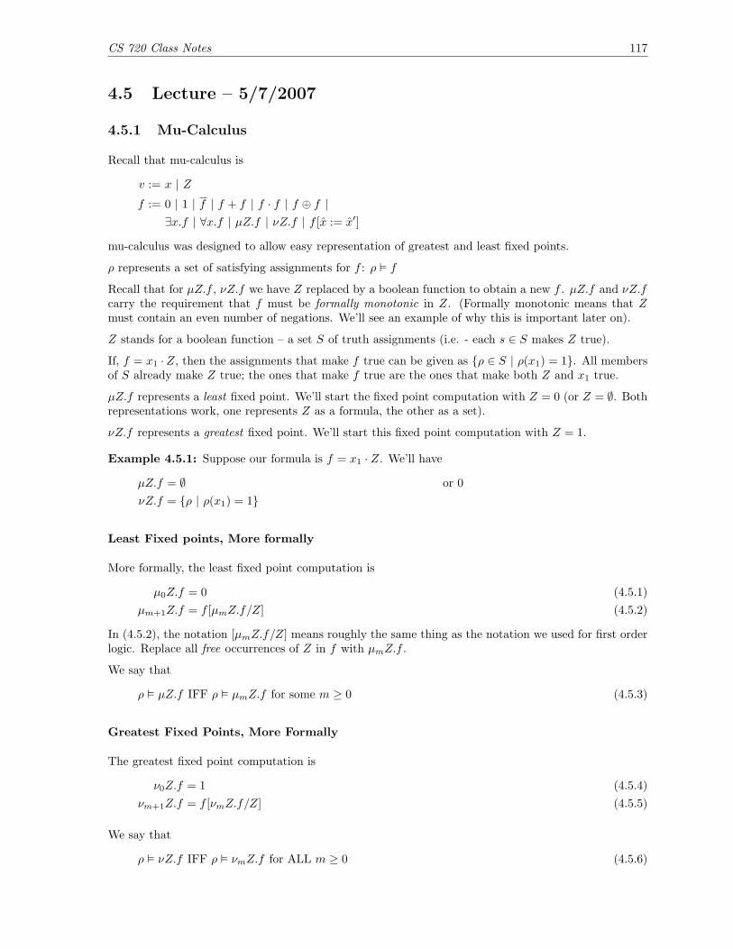
CS 720 Class Notes 117
4.5 Lecture – 5/7/2007
4.5.1 Mu-Calculus
Recall that mu-calculus is
v := x | Zf := 0 | 1 | f | f + f | f · f | f ⊕ f |
∃x.f | ∀x.f | µZ.f | νZ.f | f [x := x′]
mu-calculus was designed to allow easy representation of greatest and least fixed points.
ρ represents a set of satisfying assignments for f : ρ � f
Recall that for µZ.f , νZ.f we have Z replaced by a boolean function to obtain a new f . µZ.f and νZ.fcarry the requirement that f must be formally monotonic in Z. (Formally monotonic means that Zmust contain an even number of negations. We’ll see an example of why this is important later on).
Z stands for a boolean function – a set S of truth assignments (i.e. - each s ∈ S makes Z true).
If, f = x1 ·Z, then the assignments that make f true can be given as {ρ ∈ S | ρ(x1) = 1}. All membersof S already make Z true; the ones that make f true are the ones that make both Z and x1 true.
µZ.f represents a least fixed point. We’ll start the fixed point computation with Z = 0 (or Z = ∅. Bothrepresentations work, one represents Z as a formula, the other as a set).
νZ.f represents a greatest fixed point. We’ll start this fixed point computation with Z = 1.
Example 4.5.1: Suppose our formula is f = x1 · Z. We’ll have
µZ.f = ∅ or 0νZ.f = {ρ | ρ(x1) = 1}
Least Fixed points, More formally
More formally, the least fixed point computation is
µ0Z.f = 0 (4.5.1)µm+1Z.f = f [µmZ.f/Z] (4.5.2)
In (4.5.2), the notation [µmZ.f/Z] means roughly the same thing as the notation we used for first orderlogic. Replace all free occurrences of Z in f with µmZ.f .
We say that
ρ � µZ.f IFF ρ � µmZ.f for some m ≥ 0 (4.5.3)
Greatest Fixed Points, More Formally
The greatest fixed point computation is
ν0Z.f = 1 (4.5.4)νm+1Z.f = f [νmZ.f/Z] (4.5.5)
We say that
ρ � νZ.f IFF ρ � νmZ.f for ALL m ≥ 0 (4.5.6)
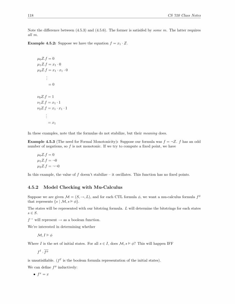
118 CS 720 Class Notes
Note the difference between (4.5.3) and (4.5.6). The former is satisifed by some m. The latter requiresall m.
Example 4.5.2: Suppose we have the equation f = x1 · Z.
µ0Z.f = 0µ1Z.f = x1 · 0µ2Z.f = x1 · x1 · 0
...= 0
ν0Z.f = 1ν1Z.f = x1 · 1ν2Z.f = x1 · x1 · 1
...= x1
In these examples, note that the formulas do not stabilize, but their meaning does.
Example 4.5.3 (The need for Formal Monotonicity): Suppose our formula was f = ¬Z. f has an oddnumber of negations, so f is not monotonic. If we try to compute a fixed point, we have
µ0Z.f = 0µ1Z.f = ¬0µ2Z.f = ¬¬0
In this example, the value of f doesn’t stabilize – it oscillates. This function has no fixed points.
4.5.2 Model Checking with Mu-Calculus
Suppose we are given M = (S,→, L), and for each CTL formula φ, we want a mu-calculus formula fφ
that represents {s | M, s � φ}.
The states will be represented with our bitstring formula. L will determine the bitstrings for each statess ∈ S.
f→ will represent → as a boolean function.
We’re interested in determining whether
M, I � φ
Where I is the set of initial states. For all s ∈ I, does M, s � φ? This will happen IFF
f I · fφ
is unsatisifiable. (f I is the boolean formula representation of the initial states).
We can define fφ inductively:
• fx = x

CS 720 Class Notes 119
• f⊥ = 0
• f¬φ = fφ
• fφ∧ψ = fφ ∧ fψ
• fφ∨ψ = fφ ∨ fψ
These are the simple cases. Formulas with path quantifiers will require a little more explanation.
fEXφ = ∃x′.(f→ · fφ[x := x′]) (4.5.7)
Recall that M, s � EXφ IFF there is an s′ where s→ s′ and s′ � φ. Equation (4.5.7) reflects this: x isthe current state, x′ is the successor state, and f→ means that there is a transition (x, x′).
The clause for EF is based on the equivalence
EFφ ≡ φ ∨ EX EFφ
fEFφ is derived from
fEFφ = fφ + fEX EFφ
= fφ + ∃x′.(f→ · fEFφ[x := x′])
= µZ.(fφ + ∃x′.(f→ · Z[x := x′]))
The last line comes about because EFφ requires a least fixed point computation.
EFφ ≡ E[>Uφ]. We can use this fact to generalize a formula for fE[φUψ]. Note that
E[φUψ] ≡ ψ ∨ (φ ∧ EX E[φUψ])
So
fE[φUψ] = fψ + fφ · fEX E[φUψ]
= fψ + fφ · ∃x′.(f→ · fE[φUψ][x := x′])
= µZ.(fψ + fφ · ∃x′.(f→ · Z[x := x′]))
The definiton of fAFφ is similar to the one for fEFφ, except that the existential quantification is replacedby universal quantification.
fAFφ = µZ.(fφ + ∀x′.(f→ + Z[x := x′]))
Finally, we’ll look at fEGφ. Recall that
EGφ ≡ φ ∧ EX EGφ
So
fEGφ = νZ.(fφ · ∃x′.(f→ · Z[x := x′]))
Tip: In a recursive equivalence, ∧ usually means we’ll need a greatest fixed point (like EGφ); ∨ usuallymeans we’ll need a least fixed point (like EFφ).

120 CS 720 Class Notes
4.5.3 Symbolic Model Checking with Fairness
In the world of CTL model checking, we want to consider paths where the fairness constraints occurinfinitely often.
LTL can express fairness constraints directly, so there’s no special handling for fairness constraints inLTL.
Given fairness constraints C = {φ1, . . . , φk}, we’d like to define mu-calculus formulas fECX, fECG, andfECU. EX, EG, and EU are an adequate set of connectives for CTL, so we can get by with only this setof definitions.
First, we define fairness as a boolean formula
fair = fECG> (4.5.8)
The idea: (4.5.8) evaluates to 1 IFF there is a fair path with respect to C that begins in the state s.
The fair version of ECX can be derived directly from fEX:
fECXφ = ∃x′.(f→ · (fφ · fair)[x := x′]) (4.5.9)
A fair version of EU can be derived similarly:
fEC[φ1 Uφ2] = µZ.(fφ2 · fair + fφ1 · ∃x′.(f→ · Z[x := x′])) (4.5.10)
Now, we just have to define fECG (which is used to define fair). We employ a pair of helper functions todo this.
checkEX(f) = ∃x′.(f→ · f [x := x′]) (4.5.11)
Equation (4.5.11) checks the EX condition. With this definition, we could rewrite fECXφ as
fECXφ = checkEX(fφ · fair)
We’ll also define a helper function for EU
checkEU(f, g) = µY.g + (f · checkEX(Y )) (4.5.12)
Finally, we code fECG:
fECGφ = νZ.fφ ·k∏i=1
checkEX(checkEU(fφ, Z · fψi) · fair) (4.5.13)
(ψi are the fairness constraints).
Note that (4.5.13) has a least fixed point (checkEU), in the body of a greatest fixed point (checkEX).Computationally, it’s a little expensive.
We can also express
ECGφ ≡ φk∧i=1
EX E[φU(ψi ∧ ECGφ)]
If ECGφ is true, then s � φ, and for each i, there is (a) a fairness constraint that is true and (b) ECGφis true somewhere later on that path.
If φ∧ki=1 EX E[φU(ψi∧ECGφ)] is true, then there is a path with φ true until ψ1 is true. From the point
where ψi is true, we can get to ψ2, etc.
Note that fairness constraints nest fixpoints.

CS 720 Class Notes 121
4.5.4 Logistics
• In the next few classes, we’ll cover material from the beginning of Chapter four.
• Our final will be a take-home exam. It will be distributed later this week, due during finals week.
Part 5
Program Verification
This material is covered in Chapter 4 of H&R
5.1 Lecture – 5/9/2007
Our look at program verification will focus on sequential programs that run on a single processor (noconcurrency). These programs can be characterized by having an infinite state space.
The classical work in program verification was done by Floyd and Hoare. Floyd’s approach used inductiveassertion. Hoare’s approach used Hoare Logic. We’ll focus on Hoare’s approach.
5.1.1 Classification of Program Verification Techniques
We’ll study techniques that are
• Proof-based. (Not the exhaustive state checking used for model verification).
• Semi-automatic.
• Property Based. We will verify certain aspects of program behavior, but not the full programbehavior.
• Application Domain. These techniques will apply to sequential transformational programs (notthe reactive systems we studied with model checking).
5.1.2 A Framework For Program Verification
• We can start with an informal specification R. R will be converted into a formal specification inthe form of a formula φR. φR is represented using some form of symbolic logic.
• We write a program P to implement R.
• We prove that P satisfies φR.
5.1.3 A Simple Programming Language
To discuss verification techniques, we’ll introduce a simple programming language. This language uses(1) integer expressions, (2) boolean expressions, and (3) control structures.
122

CS 720 Class Notes 123
Although simple, it’s really sufficient to represent any computable function (although it won’t be veryconvenient to do so).
Integer Expressions
E ::= n | x | (−E) | (E + E) | (E − E) | (E × E) (5.1.1)
Above, n is an integer (n ∈ Z). x is any program variable.
Boolean Expressions
B ::= true | false | (!B) | (B&B) | (B||B) | (E < E) (5.1.2)
(E < E) is our only native integer test. For notational convenience, we’ll use == and !=, with theknowledge that these tests could be implemented as
!(E1 < E2) & !(E2 < E1) and(E1 < E2) || (E2 < E1)
respectively.
Control Structures
Our control structures are
C ::= x = E | C;C | if B {C1} else {C2} | while B {C} (5.1.3)
while is our only looping construct.
Here’s an example of a program (which computes x!).
Example 5.1.1 (Fac1):
y = 1;z = 0;while (z != x) {z = z + 1;y = y * z;
}
There’s no return statement. That’s okay. We’re really interested in the properties that variables havebefore and after execution.
5.1.4 Hoare Triples
All programs have a starting state (before execution), and an ending state (after execution). Here, statecan be thought of as a vector of variables.
We will make assertions using Hoare triples. Hoare triples have the following form:
LφMP LψM (5.1.4)
In (5.1.4),
• φ is precondition (in first-order logic)
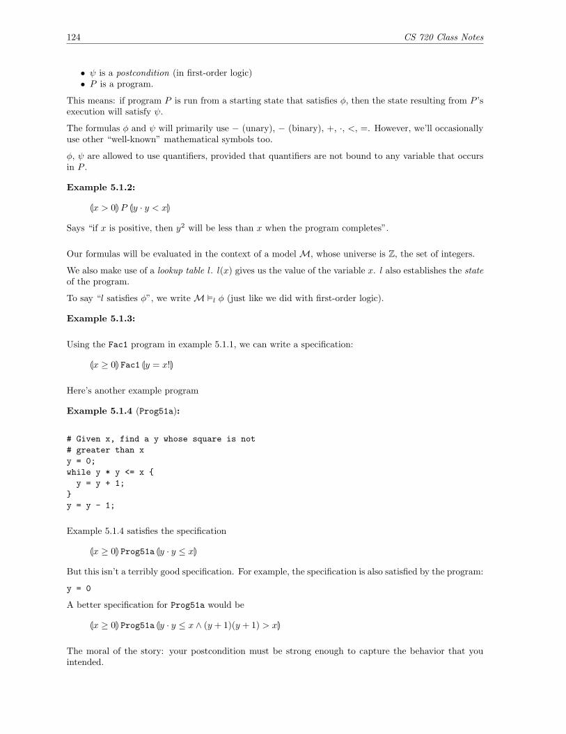
124 CS 720 Class Notes
• ψ is a postcondition (in first-order logic)• P is a program.
This means: if program P is run from a starting state that satisfies φ, then the state resulting from P ’sexecution will satisfy ψ.
The formulas φ and ψ will primarily use − (unary), − (binary), +, ·, <, =. However, we’ll occasionallyuse other “well-known” mathematical symbols too.
φ, ψ are allowed to use quantifiers, provided that quantifiers are not bound to any variable that occursin P .
Example 5.1.2:
Lx > 0MP Ly · y < xM
Says “if x is positive, then y2 will be less than x when the program completes”.
Our formulas will be evaluated in the context of a model M, whose universe is Z, the set of integers.
We also make use of a lookup table l. l(x) gives us the value of the variable x. l also establishes the stateof the program.
To say “l satisfies φ”, we write M �l φ (just like we did with first-order logic).
Example 5.1.3:
Using the Fac1 program in example 5.1.1, we can write a specification:
Lx ≥ 0M Fac1 Ly = x!M
Here’s another example program
Example 5.1.4 (Prog51a):
# Given x, find a y whose square is not# greater than xy = 0;while y * y <= x {y = y + 1;
}y = y - 1;
Example 5.1.4 satisfies the specification
Lx ≥ 0M Prog51a Ly · y ≤ xM
But this isn’t a terribly good specification. For example, the specification is also satisfied by the program:
y = 0
A better specification for Prog51a would be
Lx ≥ 0M Prog51a Ly · y ≤ x ∧ (y + 1)(y + 1) > xM
The moral of the story: your postcondition must be strong enough to capture the behavior that youintended.

CS 720 Class Notes 125
Types of Correctness
Definition 5.1.5 (Partial Correctness): LφMP LψM is correct under partial correctness if, whenever P isstarted in a state where φ is true and P halts, then ψ is true in the final state of P .
We write this `par LφMP LψM.
Partial Correctness is a weak concept: a program that never terminates satisfies any specification underpartial correctness. For example:
LφM while true { x = x } LψM
is true for any φ, ψ.
Definition 5.1.6 (Total Correctness): LφMP LψM is correct under total correctness if, whenever P isstarted in a state that makes φ true, P terminates, and ψ is true in the final state of P .
We write this `tot LφMP LψM
This is a stronger concept. Given our earlier infinite loop program P , P is not totally correct if it startswith φ true. However, if P is started with φ false, then P is totally correct.
The traditional way to prove total correctness is a two-step process
1. Prove that P is partially correct2. Prove that P terminates.
We can think of total correctness as
total correctness = partial correctness + termination
Example 5.1.7: Some examples of total and partial correctness, using our Fac1 program (example5.1.1).
�tot Lx > 0M Fac1 Ly = x!M holds2tot LtrueM Fac1 Ly = x!M Doesn’t hold when x < 0 (wrong answer)�par LtrueM Fac1 Ly = x!M Holds - the program never halts
5.1.5 Soundness and Completeness
As with first-order logic, Hoare logic has notions of soundness and completeness.
`par,`tot Soundness, a syntactic notion�par,�tot Completeness, a semantic notion
Although we won’t prove it, Hoare logic is sound and complete:
`par . . .⇒ �par
`tot . . .⇒ �tot
�par . . .⇒ `par
�tot . . .⇒ `tot

126 CS 720 Class Notes
5.1.6 Logical Variables
Let’s consider another program:
Example 5.1.8 (Fac2):
y = 1;while x != 0 {y = y * x;x = x + 1;
}
This program also computes factorial. Note that it modifies (“consumes”) the input variable x. Becausex is consumed, the postcondition we’d want, Ly = x!M, doesn’t hold.
We’ll handle this by adding logical variables. Logical variables are used to preserve program input,enabling one to use those values when reasoning about the program output. Example:
Lx ≥ 0 ∧ x = x0M Fac2 Ly = x0!M
Above, x0 is a logical variable. This is not an assignment. The clause x = x0 means “we start theprogram from a state where the logical variable x0 has the same value as the program variable x”.
By using logical variables, we can make the specification work without changing the program.
Only logical variables can be quantified.
5.1.7 A Proof Calculus for Partial Correctness
Below are the syntactic rules for Hoare Logic.
LφMC1 LηM LηMC2 LψMLφMC1;C2 LψM
Composition
Lψ[E/x]Mx = E LψMAssignment
Lφ ∧BMC1 LψM Lφ ∧ ¬BMC2 LψMLφM if B{C1} else {C2} LψM
If-statement
Lψ ∧BMC LψMLψM while B{C} Lψ ∧ ¬BM
Partial-While
`AR φ′ → φ LφMC LψM `AR ψ → ψ′
Lφ′MC Lψ′MImplied
A few of these rules require some explanation.
Composition η acts like an intermediate state, called a mid-condition. Think of η as the place whereC1 ends and C2 picks up.

CS 720 Class Notes 127
Assignment Assignment is an axiom in our system. It’s written the opposite of what one might expect.Suppose the assignment rule were
LφMx = E Lφ[E/x]MWRONG definition for assignment
If, so - we could derive
Lx = 2Mx = y Ly = 2M
That’s obviously wrong: if we never assign to y, we can’t make any statements about it’s value.
Using the correct definition:
Lx[y/x] = 2Mx = y Ly = 2M
it works – we change x to y in the postcondition, then y = 2 will hold in the output.
If-Statement Notice that we have two cases to consider: those where B holds and those where ¬Bholds. Either way, we expect to satisfy the same postconditions.
Partial-While We start by assuming B is true (if not, C never executes). We also require ¬B whenthe loop terminates.
This construct only holds under partial correctness.
Implies AR stands for “arithmetic”. This rule allows us to draw conclusions by mathematically ma-nipulating the precondition and postcondition.
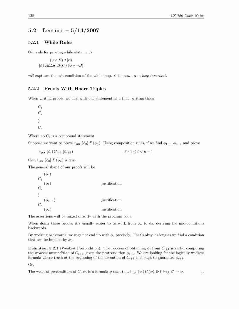
128 CS 720 Class Notes
5.2 Lecture – 5/14/2007
5.2.1 While Rules
Our rule for proving while statements:
Lψ ∧BM C LψMLψM while B{C} Lψ ∧ ¬BM
¬B captures the exit condition of the while loop. ψ is known as a loop invariant .
5.2.2 Proofs With Hoare Triples
When writing proofs, we deal with one statement at a time, writing them
C1
C2
...Cn
Where no Ci is a compound statement.
Suppose we want to prove `par Lφ0MP LφnM. Using composition rules, if we find φ1 . . . φn−1 and prove
`par LφiMCi+1 Lφi+1M for 1 ≤ i < n− 1
then `par Lφ0MP LφnM is true.
The general shape of our proofs will be
Lφ0MC1
Lφ1M justificationC2
...Lφn−1M justification
CnLφnM justification
The assertions will be mixed directly with the program code.
When doing these proofs, it’s usually easier to to work from φn to φ0, deriving the mid-conditionsbackwards.
By working backwards, we may not end up with φ0 precisely. That’s okay, as long as we find a conditionthat can be implied by φ0.
Definition 5.2.1 (Weakest Precondition): The process of obtaining φi from Ci+1 is called computingthe weakest precondition of Ci+1, given the postcondition φi+1. We are looking for the logically weakestformula whose truth at the beginning of the execution of Ci+1 is enough to guarantee φi+1.
Or,
The weakest precondition of C, ψ, is a formula φ such that �par Lφ′MC LψM IFF `AR φ′ → φ.

CS 720 Class Notes 129
Given φ′ → φ, φ is weaker. We want φ to be the weakest formula that ensures LφMP LψM.
This is really our Implied rule:
` φ′ → φ, LφMC LψM, ` ψ → ψ′
Lφ′MC Lψ′M
5.2.3 The Assignment Rule
Recall the assignment rule (an axiom)
Lψ[E/x]Mx = E LψM
Example 5.2.2: We show that `par Ly = 5M x = y + 1 Lx = 6M is valid.
Ly = 5MLy + 1 = 6M Implied
x = y + 1Lx = 6M Assignment
Note how we used the assignment rule to get from x = 6 to y + 1 = 6. (x = 6)[y + 1/x] = y + 1 = 6.
Also note the use of Implied. (y = 5)→ (y + 1 = 6).
If our proof takes the shape
φ1 → φ, LφMC LψMLφ1MC LψM
(5.2.1)
This is still the implied rule. If we wrote the last step explicitly, it would be ψ → ψ.
Example 5.2.3 (Swapping variables): Let us define the program swap:
t = x;x = y;y = t;
We want to prove Lx = x0 ∧ y = y0M swap Lx = y0 ∧ y = x0M
Lx = x0 ∧ y = y0MLy = y0 ∧ x = x0M Implication
t = xLy = y0 ∧ t = x0M Assignment
x = yLx = y0 ∧ t = x0M Assignment
y = tLx = y0 ∧ y = x0M Assignment
The key thing to notice: with the Assignment rule, the assertions are derived mechanically. It’s asyntactic derivation – just like natural deduction.
To do: try this with a “broken” swap program, and see why the proof doesn’t work.
5.2.4 If Statements
We want to derive the weakest precondition of
LφM if B{C1} else {C2} LψM
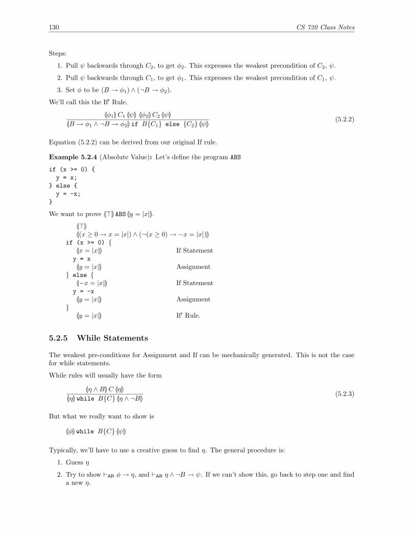
130 CS 720 Class Notes
Steps:
1. Pull ψ backwards through C2, to get φ2. This expresses the weakest precondition of C2, ψ.
2. Pull ψ backwards through C1, to get φ1. This expresses the weakest precondition of C1, ψ.
3. Set φ to be (B → φ1) ∧ (¬B → φ2).
We’ll call this the If′ Rule.
Lφ1MC1 LψM Lφ2MC2 LψMLB → φ1 ∧ ¬B → φ2M if B{C1} else {C2} LψM
(5.2.2)
Equation (5.2.2) can be derived from our original If rule.
Example 5.2.4 (Absolute Value): Let’s define the program ABS
if (x >= 0) {y = x;
} else {y = -x;
}
We want to prove L>M ABS Ly = |x|M.
L>ML(x ≥ 0→ x = |x|) ∧ (¬(x ≥ 0)→ −x = |x|)M
if (x >= 0) {Lx = |x|M If Statementy = xLy = |x|M Assignment
} else {L−x = |x|M If Statementy = -xLy = |x|M Assignment
}Ly = |x|M If′ Rule.
5.2.5 While Statements
The weakest pre-conditions for Assignment and If can be mechanically generated. This is not the casefor while statements.
While rules will usually have the form
Lη ∧BMC LηMLηM while B{C} Lη ∧ ¬BM
(5.2.3)
But what we really want to show is
LφM while B{C} LψM
Typically, we’ll have to use a creative guess to find η. The general procedure is:
1. Guess η
2. Try to show `AR φ→ η, and `AR η ∧ ¬B → ψ. If we can’t show this, go back to step one and finda new η.

CS 720 Class Notes 131
3. Pull η back through C to get η′
4. Try to find ` (η∧B)→ η′. If that’s not possible, go back to step (1) and pick a new η. Otherwise,the selection of η worked.
Example 5.2.5 (Factorial #1): Let’s define the program Fac1 as
y = 1;x = 0;while (z != x) {z = z + 1;y = y * z;
}
We want to show L>M Fac1 Ly = x! ∧ z ≥ 0M. Let us chose η : (y = z! ∧ z ≥ 0).
L>ML1 = 0! ∧ 0 ≥ 0M Implication
y = 1Ly = 0! ∧ 0 ≥ 0M Assignment
z = 0Ly = z! ∧ z ≥ 0M Assignment
while (z != x) {Ly = z! ∧ z ≥ 0 ∧ z 6= xMLy · (z + 1) = (z + 1)! ∧ (z + 1) ≥ 0M Implicationz = z + 1Ly · z = z! ∧ z ≥ 0M Assignmenty = y * zLy = z! ∧ z ≥ 0M Assignment
}Ly = z! ∧ z ≥ 0 ∧ ¬¬(z = x)M WhileLy = x!M Implication
Example 5.2.6 (Factorial #2): Let us define the program Fac2:
y = 1;while (x != 0) {y = y * x;x = x - 1;
}
We’ll want to prove
Lx = x0M Fac2 Ly = x0!M
Our invariant will be
η : x ≥ 0→ y · x! = x0! (5.2.4)
We’ll continue this example in our next lecture.
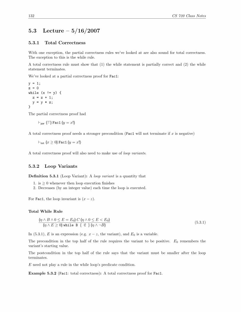
132 CS 720 Class Notes
5.3 Lecture – 5/16/2007
5.3.1 Total Correctness
With one exception, the partial correctness rules we’ve looked at are also sound for total correctness.The exception to this is the while rule.
A total correctness rule must show that (1) the while statement is partially correct and (2) the whilestatement terminates.
We’ve looked at a partial correctness proof for Fac1:
y = 1;z = 0while (x != y) {z = z + 1;y = y * z;
}
The partial correctness proof had
`par L>M Fac1 Ly = x!M
A total correctness proof needs a stronger precondition (Fac1 will not terminate if x is negative)
`tot Lx ≥ 0M Fac1 Ly = x!M
A total correctness proof will also need to make use of loop variants.
5.3.2 Loop Variants
Definition 5.3.1 (Loop Variant): A loop variant is a quantity that
1. is ≥ 0 whenever then loop execution finishes2. Decreases (by an integer value) each time the loop is executed.
For Fac1, the loop invariant is (x− z).
Total While Rule
Lη ∧B ∧ 0 ≤ E = E0MC Lη ∧ 0 ≤ E < E0MLη ∧ E ≥ 0M while B { C } Lη ∧ ¬BM
(5.3.1)
In (5.3.1), E is an expression (e.g. x− z, the variant), and E0 is a variable.
The precondition in the top half of the rule requires the variant to be positive. E0 remembers thevariant’s starting value.
The postcondition in the top half of the rule says that the variant must be smaller after the loopterminates.
E need not play a rule in the while loop’s predicate condition.
Example 5.3.2 (Fac1: total correctness): A total correctness proof for Fac1.

CS 720 Class Notes 133
L0 ≥ 0 ∧ 1 = 0! ∧ x ≥ 0 ∧ 0 ≤ x− 0My = 1
L0 ≥ 0 ∧ y = 0! ∧ x ≥ 0 ∧ 0 ≤ x− 0Mz = 0
Lz ≥ 0 ∧ y = z! ∧ x ≥ 0 ∧ 0 ≤ x− zMwhile (x 6= z) {
Lz ≥ 0 ∧ y = z! ∧ x ≥ 0 ∧ 0 ≤ x− z = E0 ∧ z 6= xM [Note 1]Lz + 1 ≥ 0 ∧ y · (z + 1) = (z + 1)! ∧ x ≥ 0 ∧ 0 ≤ x− (z + 1) ≤ E0M
z = z + 1Lz ≥ 0 ∧ y · z = z! ∧ x ≥ 0 ∧ 0 ≤ x− z < E0M
y = y + zLz ≥ 0 ∧ y = z! ∧ x ≥ 0 ∧ 0 ≤ x− z < E0M
}Lz ≥ 0 ∧ y = z! ∧ ¬(x 6= z) ∧ x ≥ 0MLy = x!M
Note 1: η is z ≥ 0 ∧ y = z! ∧ x ≥ 0.0 ≤ x− z = E0 captures the loop variant, (x− z).z 6= x is B.
5.3.3 Working With Arrays
In a formal proof system, arrays can be tricky to work with. For example, given a[i] = a[j], what ifi = j?
We’ll notate arrays as
a[0] . . . a[n− 1]
Let’s define a section of an array to be a consecutive series of elements, a[i] . . . a[j] such that i ≤ j.
We’d like to find the minimal section sum for the array. What is the smallest number that can bederived from summing elements in a section?
For example, given the array [−1, 2,−3, 5, 4,−3], the minimal section sum is−3. Given [−1, 2,−3, 1, 1,−3],the minimal section sum is −4.
The naive approach would be to try all possible sections; a runtime complexity of Θ(n3). But we cando better, in Θ(n) time.
Let
s = the minimal section sum up the current point kt = the minimal section sum up to and including the current point k.
Given current values s, t, we compute the next values s′, t′ as follows:
s′ = min(s, a[k + 1], a[k + 1] + t)t′ = min(a[k + 1], a[k + 1] + 1)
The algorithm Min-sum is
k = 1;s = a[0];t = a[0];

134 CS 720 Class Notes
while (k != n) {t = min(a[k + 1], a[k + 1] + t);s = min(s, t);k = k + 1;
}/* s holds final result */
Suppose we wanted to formally verify this algorithm. Let us denote
Sij =j∑k=i
a[k]
We would use two postconditions:
Ln ≥ 0M Min-sum L∀i, j(0 ≤ i ≤ j < n→ s ≤ Sij)MLn ≥ 0M Min-sum L∃i, j(0 ≤ i ≤ j < n ∧ s = Sij)M
The first postcondition states that s is ≤ any section sum. The second postcondition states that s isthe sum of some section.
This example illustrates how modularity can be introduced into the verification process. We have acommon set of preconditions and a pair of post conditions. The two postconditions can be provenindependantly.
To prove the ∀ part, we’ll define a few shorthand notations:
Inv1(s, k) = ∀i, j(0 ≤ i ≤ j < k → s ≤ Sij)Inv2(t, k) = ∀i(0 ≤ i < k → t ≤ Si,k−1)
With these helpers, the loop invariant is
L0 ≤ k ≤ n ∧ Inv1(s, k) ∧ Inv2(t, k)M
For the ∃ part, we’d do a similar thing:
Inv1′(s, k) = ∃i, j(0 ≤ i ≤ j < k ∧ s = Sij)
(There’d also be an Inv2′ and another loop invariant).
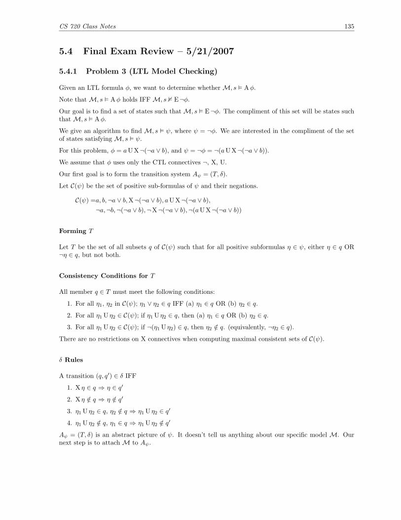
CS 720 Class Notes 135
5.4 Final Exam Review – 5/21/2007
5.4.1 Problem 3 (LTL Model Checking)
Given an LTL formula φ, we want to determine whether M, s � Aφ.
Note that M, s � Aφ holds IFF M, s 2 E¬φ.
Our goal is to find a set of states such thatM, s � E¬φ. The compliment of this set will be states suchthat M, s � Aφ.
We give an algorithm to find M, s � ψ, where ψ = ¬φ. We are interested in the compliment of the setof states satisfying M, s � ψ.
For this problem, φ = aU X¬(¬a ∨ b), and ψ = ¬φ = ¬(aU X¬(¬a ∨ b)).
We assume that φ uses only the CTL connectives ¬, X, U.
Our first goal is to form the transition system Aψ = (T, δ).
Let C(ψ) be the set of positive sub-formulas of ψ and their negations.
C(ψ) =a, b,¬a ∨ b,X¬(¬a ∨ b), aU X¬(¬a ∨ b),¬a,¬b,¬(¬a ∨ b),¬X¬(¬a ∨ b),¬(aU X¬(¬a ∨ b))
Forming T
Let T be the set of all subsets q of C(ψ) such that for all positive subformulas η ∈ ψ, either η ∈ q OR¬η ∈ q, but not both.
Consistency Conditions for T
All member q ∈ T must meet the following conditions:
1. For all η1, η2 in C(ψ); η1 ∨ η2 ∈ q IFF (a) η1 ∈ q OR (b) η2 ∈ q.
2. For all η1 U η2 ∈ C(ψ); if η1 U η2 ∈ q, then (a) η1 ∈ q OR (b) η2 ∈ q.
3. For all η1 U η2 ∈ C(ψ); if ¬(η1 U η2) ∈ q, then η2 /∈ q. (equivalently, ¬η2 ∈ q).
There are no restrictions on X connectives when computing maximal consistent sets of C(ψ).
δ Rules
A transition (q, q′) ∈ δ IFF
1. X η ∈ q ⇒ η ∈ q′
2. X η /∈ q ⇒ η /∈ q′
3. η1 U η2 ∈ q, η2 /∈ q ⇒ η1 U η2 ∈ q′
4. η1 U η2 /∈ q, η1 ∈ q ⇒ η1 U η2 /∈ q′
Aψ = (T, δ) is an abstract picture of ψ. It doesn’t tell us anything about our specific model M. Ournext step is to attach M to Aψ.

136 CS 720 Class Notes
Forming M×Aψ
We define M×Aψ = (U, δ′), where
U = {(s, q) ∈ S × T | for all atoms p ∈ C(ψ), p ∈ q IFF p ∈ L(s)}
Using problem 3 as an example, if our state is q = 00100, then ¬a ∈ q and ¬b ∈ q. We must pair q witha state s of M where s has a /∈ L(s) and b /∈ L(s).
Whatever M says about atoms in s, q must say the same things about atoms in C(ψ).
Next, the transition relation δ′.
δ′ = {(s, q)→ (s′, q′) | s→ s′ ∈M and q → q′ ∈ δ}
In other words, the transition relations of M and Aψ must be in agreement.
Strongly Connected Components
Next, we’ll find the strongly connected components of M× Aψ. There are algorithms that accomplishthis task. For our purpose, eyeballing M×Aψ will be sufficient.
A strongly connected component C is a connected component where the following is true: from eachnode in C, you can get to every other node in C.
The set of strongly connected components forms a partition of a graph. A trivial SCC cannot be partof a non-trivial SCC. Figure 5.1 shows a graph with 1 Trivial SCC and two non-trivial SCCs.
Trivial
Non−Trivial
Non−Trivial
Figure 5.1: Graph with 1 trivial and 2 non-trivial SCCs
Self Fulfilling SCC
A strongly connected component ofM×Aψ is self fulfilling if, for all η1 U η2 that are in some SCC node(s, q), η2 is in some node (s′, q′) of the SCC.
If η1 U η2 does not occur in any SCC component, then this condition is vacuously true (the SCC is selffulfilling).
M, s � Eψ IFF there is a path from an (s, q) (with ψ ∈ q) in M× Aψ, to a non-trivial self-fulfillingSCC of M×Aψ.

CS 720 Class Notes 137
Additional Notes
Assuming φ is positive, Aφ and A¬φ will produce the same model, so Aφ = A¬φ for a positive φ.
In the last step (self-fulfilling SCC), we are looking for ψ = ¬φ.
We find E¬φ in order to find Aφ.
5.4.2 Problem 4
The definition of “active assumption” will involve boxes. We can assume that the proof has properlynested boxes.
5.4.3 Problem 5
A Greatest fixed point proof involves two things
1. K(JECGφK) = JECGφK.
2. If K(X) = X, then X ⊆ JECGφK.
The first step shows that JECGφK is a fixed point of K. The second step shows that it is the greatestfixed point of K.

138 CS 720 Class Notes
GNU Free Documentation License
Version 1.2, November 2002
Copyright c© 2000,2001,2002 Free Software Foundation, Inc.
51 Franklin St, Fifth Floor, Boston, MA 02110-1301 USA
Everyone is permitted to copy and distribute verbatim copies of this license document, but changing itis not allowed.
Preamble
The purpose of this License is to make a manual, textbook, or other functional and useful document“free” in the sense of freedom: to assure everyone the effective freedom to copy and redistribute it, withor without modifying it, either commercially or noncommercially. Secondarily, this License preserves forthe author and publisher a way to get credit for their work, while not being considered responsible formodifications made by others.
This License is a kind of “copyleft”, which means that derivative works of the document must themselvesbe free in the same sense. It complements the GNU General Public License, which is a copyleft licensedesigned for free software.
We have designed this License in order to use it for manuals for free software, because free softwareneeds free documentation: a free program should come with manuals providing the same freedoms thatthe software does. But this License is not limited to software manuals; it can be used for any textualwork, regardless of subject matter or whether it is published as a printed book. We recommend thisLicense principally for works whose purpose is instruction or reference.
1. APPLICABILITY AND DEFINITIONSThis License applies to any manual or other work, in any medium, that contains a notice placed bythe copyright holder saying it can be distributed under the terms of this License. Such a notice grantsa world-wide, royalty-free license, unlimited in duration, to use that work under the conditions statedherein. The “Document”, below, refers to any such manual or work. Any member of the public is alicensee, and is addressed as “you”. You accept the license if you copy, modify or distribute the workin a way requiring permission under copyright law.
A “Modified Version” of the Document means any work containing the Document or a portion of it,either copied verbatim, or with modifications and/or translated into another language.
A “Secondary Section” is a named appendix or a front-matter section of the Document that dealsexclusively with the relationship of the publishers or authors of the Document to the Document’s overallsubject (or to related matters) and contains nothing that could fall directly within that overall subject.(Thus, if the Document is in part a textbook of mathematics, a Secondary Section may not explainany mathematics.) The relationship could be a matter of historical connection with the subject or withrelated matters, or of legal, commercial, philosophical, ethical or political position regarding them.
139

140 CS 720 Class Notes
The “Invariant Sections” are certain Secondary Sections whose titles are designated, as being those ofInvariant Sections, in the notice that says that the Document is released under this License. If a sectiondoes not fit the above definition of Secondary then it is not allowed to be designated as Invariant. TheDocument may contain zero Invariant Sections. If the Document does not identify any Invariant Sectionsthen there are none.
The “Cover Texts” are certain short passages of text that are listed, as Front-Cover Texts or Back-Cover Texts, in the notice that says that the Document is released under this License. A Front-CoverText may be at most 5 words, and a Back-Cover Text may be at most 25 words.
A “Transparent” copy of the Document means a machine-readable copy, represented in a format whosespecification is available to the general public, that is suitable for revising the document straightforwardlywith generic text editors or (for images composed of pixels) generic paint programs or (for drawings)some widely available drawing editor, and that is suitable for input to text formatters or for automatictranslation to a variety of formats suitable for input to text formatters. A copy made in an otherwiseTransparent file format whose markup, or absence of markup, has been arranged to thwart or discouragesubsequent modification by readers is not Transparent. An image format is not Transparent if used forany substantial amount of text. A copy that is not “Transparent” is called “Opaque”.
Examples of suitable formats for Transparent copies include plain ASCII without markup, Texinfo inputformat, LaTeX input format, SGML or XML using a publicly available DTD, and standard-conformingsimple HTML, PostScript or PDF designed for human modification. Examples of transparent imageformats include PNG, XCF and JPG. Opaque formats include proprietary formats that can be read andedited only by proprietary word processors, SGML or XML for which the DTD and/or processing toolsare not generally available, and the machine-generated HTML, PostScript or PDF produced by someword processors for output purposes only.
The “Title Page” means, for a printed book, the title page itself, plus such following pages as areneeded to hold, legibly, the material this License requires to appear in the title page. For works informats which do not have any title page as such, “Title Page” means the text near the most prominentappearance of the work’s title, preceding the beginning of the body of the text.
A section “Entitled XYZ” means a named subunit of the Document whose title either is precisely XYZor contains XYZ in parentheses following text that translates XYZ in another language. (Here XYZstands for a specific section name mentioned below, such as “Acknowledgements”, “Dedications”,“Endorsements”, or “History”.) To “Preserve the Title” of such a section when you modify theDocument means that it remains a section “Entitled XYZ” according to this definition.
The Document may include Warranty Disclaimers next to the notice which states that this Licenseapplies to the Document. These Warranty Disclaimers are considered to be included by reference inthis License, but only as regards disclaiming warranties: any other implication that these WarrantyDisclaimers may have is void and has no effect on the meaning of this License.
2. VERBATIM COPYINGYou may copy and distribute the Document in any medium, either commercially or noncommercially,provided that this License, the copyright notices, and the license notice saying this License applies tothe Document are reproduced in all copies, and that you add no other conditions whatsoever to those ofthis License. You may not use technical measures to obstruct or control the reading or further copyingof the copies you make or distribute. However, you may accept compensation in exchange for copies. Ifyou distribute a large enough number of copies you must also follow the conditions in section 3.
You may also lend copies, under the same conditions stated above, and you may publicly display copies.
3. COPYING IN QUANTITYIf you publish printed copies (or copies in media that commonly have printed covers) of the Document,numbering more than 100, and the Document’s license notice requires Cover Texts, you must enclose
CS 720 Class Notes 141
the copies in covers that carry, clearly and legibly, all these Cover Texts: Front-Cover Texts on the frontcover, and Back-Cover Texts on the back cover. Both covers must also clearly and legibly identify you asthe publisher of these copies. The front cover must present the full title with all words of the title equallyprominent and visible. You may add other material on the covers in addition. Copying with changeslimited to the covers, as long as they preserve the title of the Document and satisfy these conditions,can be treated as verbatim copying in other respects.
If the required texts for either cover are too voluminous to fit legibly, you should put the first ones listed(as many as fit reasonably) on the actual cover, and continue the rest onto adjacent pages.
If you publish or distribute Opaque copies of the Document numbering more than 100, you must eitherinclude a machine-readable Transparent copy along with each Opaque copy, or state in or with eachOpaque copy a computer-network location from which the general network-using public has access todownload using public-standard network protocols a complete Transparent copy of the Document, freeof added material. If you use the latter option, you must take reasonably prudent steps, when youbegin distribution of Opaque copies in quantity, to ensure that this Transparent copy will remain thusaccessible at the stated location until at least one year after the last time you distribute an Opaque copy(directly or through your agents or retailers) of that edition to the public.
It is requested, but not required, that you contact the authors of the Document well before redistributingany large number of copies, to give them a chance to provide you with an updated version of theDocument.
4. MODIFICATIONSYou may copy and distribute a Modified Version of the Document under the conditions of sections 2 and3 above, provided that you release the Modified Version under precisely this License, with the ModifiedVersion filling the role of the Document, thus licensing distribution and modification of the ModifiedVersion to whoever possesses a copy of it. In addition, you must do these things in the Modified Version:
A. Use in the Title Page (and on the covers, if any) a title distinct from that of the Document, andfrom those of previous versions (which should, if there were any, be listed in the History section ofthe Document). You may use the same title as a previous version if the original publisher of thatversion gives permission.
B. List on the Title Page, as authors, one or more persons or entities responsible for authorship ofthe modifications in the Modified Version, together with at least five of the principal authors ofthe Document (all of its principal authors, if it has fewer than five), unless they release you fromthis requirement.
C. State on the Title page the name of the publisher of the Modified Version, as the publisher.
D. Preserve all the copyright notices of the Document.
E. Add an appropriate copyright notice for your modifications adjacent to the other copyright notices.
F. Include, immediately after the copyright notices, a license notice giving the public permission touse the Modified Version under the terms of this License, in the form shown in the Addendumbelow.
G. Preserve in that license notice the full lists of Invariant Sections and required Cover Texts givenin the Document’s license notice.
H. Include an unaltered copy of this License.
I. Preserve the section Entitled “History”, Preserve its Title, and add to it an item stating at leastthe title, year, new authors, and publisher of the Modified Version as given on the Title Page. Ifthere is no section Entitled “History” in the Document, create one stating the title, year, authors,and publisher of the Document as given on its Title Page, then add an item describing the ModifiedVersion as stated in the previous sentence.
142 CS 720 Class Notes
J. Preserve the network location, if any, given in the Document for public access to a Transparentcopy of the Document, and likewise the network locations given in the Document for previousversions it was based on. These may be placed in the “History” section. You may omit a networklocation for a work that was published at least four years before the Document itself, or if theoriginal publisher of the version it refers to gives permission.
K. For any section Entitled “Acknowledgements” or “Dedications”, Preserve the Title of the section,and preserve in the section all the substance and tone of each of the contributor acknowledgementsand/or dedications given therein.
L. Preserve all the Invariant Sections of the Document, unaltered in their text and in their titles.Section numbers or the equivalent are not considered part of the section titles.
M. Delete any section Entitled “Endorsements”. Such a section may not be included in the ModifiedVersion.
N. Do not retitle any existing section to be Entitled “Endorsements” or to conflict in title with anyInvariant Section.
O. Preserve any Warranty Disclaimers.
If the Modified Version includes new front-matter sections or appendices that qualify as SecondarySections and contain no material copied from the Document, you may at your option designate someor all of these sections as invariant. To do this, add their titles to the list of Invariant Sections in theModified Version’s license notice. These titles must be distinct from any other section titles.
You may add a section Entitled “Endorsements”, provided it contains nothing but endorsements of yourModified Version by various parties–for example, statements of peer review or that the text has beenapproved by an organization as the authoritative definition of a standard.
You may add a passage of up to five words as a Front-Cover Text, and a passage of up to 25 words asa Back-Cover Text, to the end of the list of Cover Texts in the Modified Version. Only one passage ofFront-Cover Text and one of Back-Cover Text may be added by (or through arrangements made by) anyone entity. If the Document already includes a cover text for the same cover, previously added by youor by arrangement made by the same entity you are acting on behalf of, you may not add another; butyou may replace the old one, on explicit permission from the previous publisher that added the old one.
The author(s) and publisher(s) of the Document do not by this License give permission to use theirnames for publicity for or to assert or imply endorsement of any Modified Version.
5. COMBINING DOCUMENTSYou may combine the Document with other documents released under this License, under the termsdefined in section 4 above for modified versions, provided that you include in the combination all of theInvariant Sections of all of the original documents, unmodified, and list them all as Invariant Sectionsof your combined work in its license notice, and that you preserve all their Warranty Disclaimers.
The combined work need only contain one copy of this License, and multiple identical Invariant Sectionsmay be replaced with a single copy. If there are multiple Invariant Sections with the same name butdifferent contents, make the title of each such section unique by adding at the end of it, in parentheses,the name of the original author or publisher of that section if known, or else a unique number. Makethe same adjustment to the section titles in the list of Invariant Sections in the license notice of thecombined work.
In the combination, you must combine any sections Entitled “History” in the various original documents,forming one section Entitled “History”; likewise combine any sections Entitled “Acknowledgements”, andany sections Entitled “Dedications”. You must delete all sections Entitled “Endorsements”.
6. COLLECTIONS OF DOCUMENTS
CS 720 Class Notes 143
You may make a collection consisting of the Document and other documents released under this License,and replace the individual copies of this License in the various documents with a single copy that isincluded in the collection, provided that you follow the rules of this License for verbatim copying of eachof the documents in all other respects.
You may extract a single document from such a collection, and distribute it individually under thisLicense, provided you insert a copy of this License into the extracted document, and follow this Licensein all other respects regarding verbatim copying of that document.
7. AGGREGATION WITH INDEPENDENT WORKSA compilation of the Document or its derivatives with other separate and independent documents orworks, in or on a volume of a storage or distribution medium, is called an “aggregate” if the copyrightresulting from the compilation is not used to limit the legal rights of the compilation’s users beyond whatthe individual works permit. When the Document is included in an aggregate, this License does notapply to the other works in the aggregate which are not themselves derivative works of the Document.
If the Cover Text requirement of section 3 is applicable to these copies of the Document, then if theDocument is less than one half of the entire aggregate, the Document’s Cover Texts may be placedon covers that bracket the Document within the aggregate, or the electronic equivalent of covers if theDocument is in electronic form. Otherwise they must appear on printed covers that bracket the wholeaggregate.
8. TRANSLATIONTranslation is considered a kind of modification, so you may distribute translations of the Documentunder the terms of section 4. Replacing Invariant Sections with translations requires special permissionfrom their copyright holders, but you may include translations of some or all Invariant Sections inaddition to the original versions of these Invariant Sections. You may include a translation of thisLicense, and all the license notices in the Document, and any Warranty Disclaimers, provided that youalso include the original English version of this License and the original versions of those notices anddisclaimers. In case of a disagreement between the translation and the original version of this Licenseor a notice or disclaimer, the original version will prevail.
If a section in the Document is Entitled “Acknowledgements”, “Dedications”, or “History”, the require-ment (section 4) to Preserve its Title (section 1) will typically require changing the actual title.
9. TERMINATIONYou may not copy, modify, sublicense, or distribute the Document except as expressly provided for underthis License. Any other attempt to copy, modify, sublicense or distribute the Document is void, and willautomatically terminate your rights under this License. However, parties who have received copies, orrights, from you under this License will not have their licenses terminated so long as such parties remainin full compliance.
10. FUTURE REVISIONS OF THIS LICENSEThe Free Software Foundation may publish new, revised versions of the GNU Free DocumentationLicense from time to time. Such new versions will be similar in spirit to the present version, but maydiffer in detail to address new problems or concerns. See http://www.gnu.org/copyleft/.
Each version of the License is given a distinguishing version number. If the Document specifies that aparticular numbered version of this License “or any later version” applies to it, you have the option offollowing the terms and conditions either of that specified version or of any later version that has beenpublished (not as a draft) by the Free Software Foundation. If the Document does not specify a versionnumber of this License, you may choose any version ever published (not as a draft) by the Free SoftwareFoundation.
Related Documents