CS5620 Geometric Modeling I Intro to Computer Graphics ·  · 2015-10-05Geometric Modeling I Page 2 7 8 Objective Methods and algorithms to mathematically model shape ... Intro to

CS5620

Intro to Computer Graphics

Copyright

C. Gotsman, G. Elber, M. Ben-Chen

Computer Science Dept., Technion

Geometric Modeling I

Page 1

Geometric

Modeling Part I

2

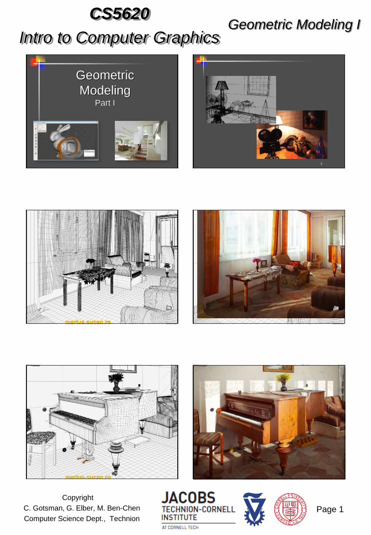
3 marius.sucan.ro

5 marius.sucan.ro 6

CS5620

Intro to Computer Graphics

Copyright

C. Gotsman, G. Elber, M. Ben-Chen

Computer Science Dept., Technion

Geometric Modeling I

Page 2

7 8

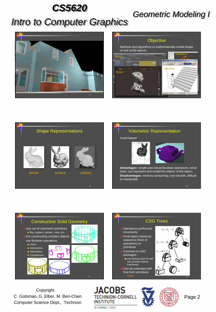
Objective

Methods and algorithms to mathematically model shape

of real world objects

Maya

MeshMixer

ZBrush

3D Studio Max

SketchUp

Shape Representations

9

points surface volume

10

Volumetric Representation

Voxel-based

Advantages: simple and robust Boolean operations, in/out

tests, can represent and model the interior of the object.

Disadvantages: memory consuming, non-smooth, difficult

to manipulate.

11

Constructive Solid Geometry

Use set of volumetric primitives

Box, sphere, cylinder, cone, etc…

For constructing complex objects

use Boolean operations

Union

Intersection

Subtraction

Complement

S S C3 2 2

S S B2 1 2

C1

B1

S B C1 1 1

12

CSG Trees

Operations performed

recursively

Final object stored as

sequence (tree) of

operations on

primitives

Common in CAD

packages –

mechanical parts fit well

into primitive based

framework

Can be extended with

free-form primitives

C2

B2

Demo

CS5620

Intro to Computer Graphics

Copyright

C. Gotsman, G. Elber, M. Ben-Chen

Computer Science Dept., Technion

Geometric Modeling I

Page 3

13

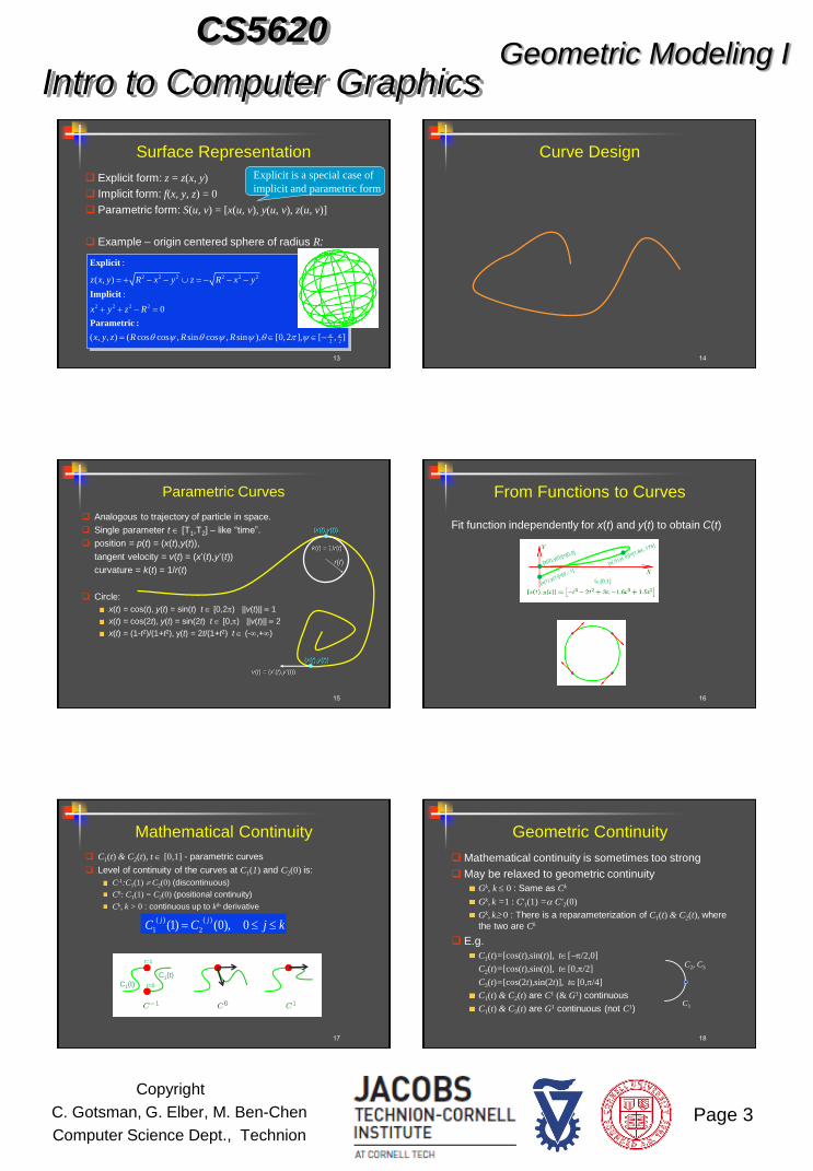
Surface Representation

Explicit form: z = z(x, y)

Implicit form: f(x, y, z) = 0

Parametric form: S(u, v) = [x(u, v), y(u, v), z(u, v)]

Example – origin centered sphere of radius R:

2 2 2 2 2 2

2 2 2 2

2 2

:

( , )

:

0

( , , ) ( cos cos , sin cos , sin ), [0,2 ], [ , ]

z x y R x y z R x y

x y z R

x y z R R R

Explicit

Implicit

Parametric :

Explicit is a special case of

implicit and parametric form

Curve Design

14

15

Parametric Curves

Analogous to trajectory of particle in space.

Single parameter t [T1,T2] – like “time”.

position = p(t) = (x(t),y(t)),

tangent velocity = v(t) = (x’(t),y’(t))

curvature = k(t) = 1/r(t)

Circle:

x(t) = cos(t), y(t) = sin(t) t [0,2) ||v(t)|| 1

x(t) = cos(2t), y(t) = sin(2t) t [0,) ||v(t)|| 2

x(t) = (1-t2)/(1+t2), y(t) = 2t/(1+t2) t (-,+)

(x(t),y(t))

v(t) = (x’(t),y’(t))

(x(t),y(t))

r(t)

k(t) = 1/r(t)

16

From Functions to Curves

Fit function independently for x(t) and y(t) to obtain C(t)

t[0,1]

17

Mathematical Continuity

C1(t) & C2(t), t [0,1] - parametric curves

Level of continuity of the curves at C1(1) and C2(0) is:

C-1:C1(1) C2(0) (discontinuous)

C0: C1(1) = C2(0) (positional continuity)

Ck, k > 0 : continuous up to kth derivative

kjCCjj

0),0()1( )(

2

)(

1

C1(t)

C1(t)

t=1

t=0

18

Geometric Continuity

Mathematical continuity is sometimes too strong

May be relaxed to geometric continuity

Gk, k 0 : Same as Ck

Gk, k =1 : C'1(1) = C'2(0)

Gk, k 0 : There is a reparameterization of C1(t) & C2(t), where

the two are Ck

E.g.

C1(t)=[cos(t),sin(t)], t[/2,0]

C2(t)=[cos(t),sin(t)], t[0,/2]

C3(t)=[cos(2t),sin(2t)], t[0,/4]

C1(t) & C2(t) are C1 (& G1) continuous

C1(t) & C3(t) are G1 continuous (not C1)

C1

C2, C3

CS5620

Intro to Computer Graphics

Copyright

C. Gotsman, G. Elber, M. Ben-Chen

Computer Science Dept., Technion

Geometric Modeling I

Page 4

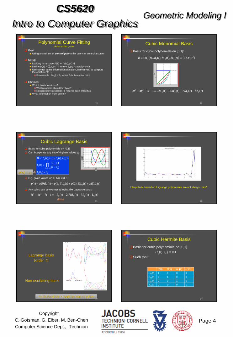
Polynomial Curve Fitting Rules of the game

Goal: Using a small set of control points the user can control a curve

Setup: Looking for a curve 𝑃 𝑡 = 𝑥 𝑡 , 𝑦 𝑡

Define 𝑃 𝑡 = 𝑐𝑖𝐵𝑖(𝑡)𝑖 , where 𝐵𝑖(𝑡) is a polynomial

Use control points information (location, derivatives) to compute the coefficients 𝑐𝑖

For example: 𝑃 𝑡𝑗 = 𝑃𝑗, where 𝑃𝑗 is the control point

Choices: Which basis functions?

What properties should they have?

Required curve properties required basis properties

What information from points?

19

Cubic Monomial Basis

20

Basis for cubic polynomials on [0,1]:

2 3

0 1 2 3{ ( ), ( ), ( ), ( )} {1, , , } B M t M t M t M t t t t

3 2

3 2 1 03 4 7 1 3 ( ) 2 ( ) 7 ( ) ( ) t t t M t M t M t M t

Cubic Lagrange Basis

Basis for cubic polynomials on [0,1]

Can interpolate any set of 4 given values pj

E.g. given values on 0, 1/3, 2/3, 1:

Any cubic can be expressed using the Lagrange basis:

21

3 2

0 1 2 33 4 7 1 ( ) 2.78 ( ) 3 ( ) ( ) t t t L t L t L t L t

0 1 2 3( ) (0) ( ) (1/ 3) ( ) (2 / 3) ( ) (1) ( ) p t p L t p L t p L t p L t

0 1 2 3

3

0,

{ ( ), ( ), ( ), ( )}

( )( )

( )

( )

j

i

j j i i j

i j ij

B L t L t L t L t

t tL t

t t

L t

Li(t)

t

demo

p 𝑡𝑗 = 𝑝𝑗

Interpolants based on Lagrange polynomials are not always “nice”

22

23

Lagrange basis

(order 7)

Non oscillating basis

Basis functions should be non-negative 24

Cubic Hermite Basis

Basis for cubic polynomials on [0,1]

Hij(t): i, j = 0,1

Such that:

H(0) H(1) H '(0) H '(1)

H00(t) 1 0 0 0

H01(t) 0 1 0 0

H10(t) 0 0 1 0

H11(t) 0 0 0 1

CS5620

Intro to Computer Graphics

Copyright

C. Gotsman, G. Elber, M. Ben-Chen

Computer Science Dept., Technion

Geometric Modeling I

Page 5

25

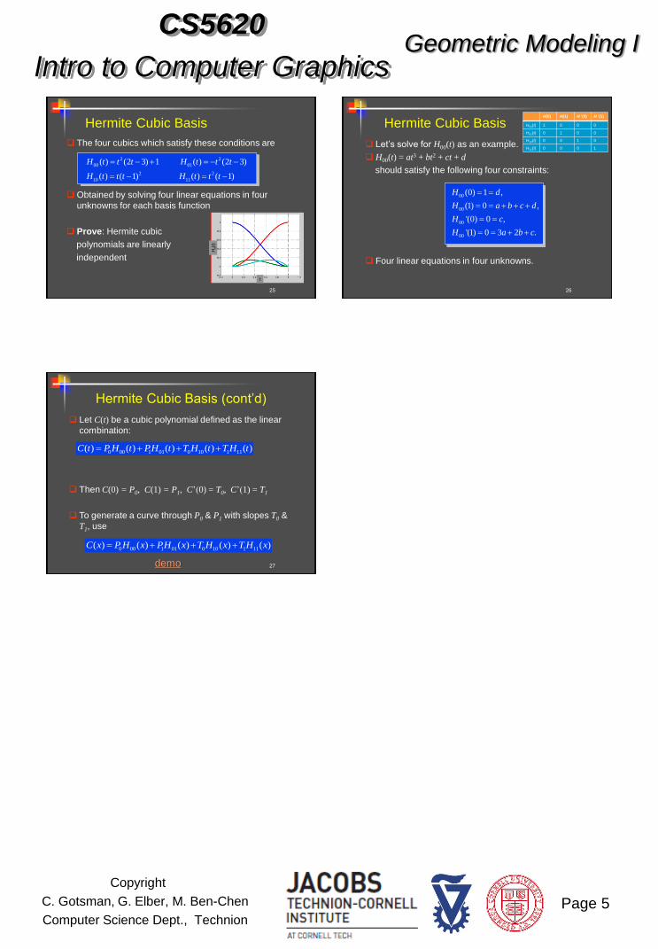
Hermite Cubic Basis

The four cubics which satisfy these conditions are

Obtained by solving four linear equations in four

unknowns for each basis function

Prove: Hermite cubic

polynomials are linearly

independent

2 2

00 01

2 2

10 11

( ) (2 3) 1 ( ) (2 3)

( ) ( 1) ( ) ( 1)

H t t t H t t t

H t t t H t t t

Hij(t

)

t

26

Hermite Cubic Basis

Let’s solve for H00(t) as an example.

H00(t) = at3 + bt2 + ct + d

should satisfy the following four constraints:

Four linear equations in four unknowns.

00

00

00

00

(0) 1 ,

(1) 0 ,

'(0) 0 ,

'(1) 0 3 2 .

H d

H a b c d

H c

H a b c

H(0) H(1) H '(0) H '(1)

H00(t) 1 0 0 0

H01(t) 0 1 0 0

H10(t) 0 0 1 0

H11(t) 0 0 0 1

27

Hermite Cubic Basis (cont’d)

Let C(t) be a cubic polynomial defined as the linear

combination:

Pi

0 00 1 01 0 10 1 11( ) ( ) ( ) ( ) ( ) C t P H t PH t T H t T H t

Then C(0) = P0, C(1) = P1, C’(0) = T0, C’(1) = T1

To generate a curve through P0 & P1 with slopes T0 &

T1, use

0 00 1 01 0 10 1 11( ) ( ) ( ) ( ) ( )C x P H x PH x T H x T H x

demo