X. Sun (IIT) CS546 Lecture 5 Page 1 Performance Evaluation of Parallel Processing Xian-He Sun Illinois Institute of T echnology [email protected]

Welcome message from author
This document is posted to help you gain knowledge. Please leave a comment to let me know what you think about it! Share it to your friends and learn new things together.
Transcript

8/2/2019 cs546perf
http://slidepdf.com/reader/full/cs546perf 1/78
X. Sun (IIT) CS546 Lecture 5 Page 1
Performance Evaluation of
Parallel Processing
Xian-He Sun
Illinois Institute of Technology

8/2/2019 cs546perf
http://slidepdf.com/reader/full/cs546perf 2/78
X. Sun (IIT) CS546 Lecture 5 Page 2
Outline
• Performance metrics – Speedup
– Efficiency
– Scalability• Examples
• Reading: Kumar – ch 5

8/2/2019 cs546perf
http://slidepdf.com/reader/full/cs546perf 3/78
X. Sun (IIT) CS546 Lecture 5 Page 3
Performance Evaluation(Improving performance is the goal)
• Performance Measurement
– Metric, Parameter
• Performance Prediction – Model, Application-Resource
• Performance Diagnose/Optimization
– Post-execution, Algorithm improvement,
Architecture improvement, State-of-the-art,Scheduling, Resource management/Scheduling

8/2/2019 cs546perf
http://slidepdf.com/reader/full/cs546perf 4/78
X. Sun (IIT) CS546 Lecture 5 Page 4
Parallel Performance Metrics(Run-time is the dominant metric)
• Run-Time (Execution Time)
• Speed: mflops, mips, cpi
• Efficiency: throughput
• Speedup
• Parallel Efficiency
• Scalability: The ability to maintain performance gain when
system and problem size increase• Others: portability, programming ability,etc
TimeExecutionParallelTimeExecutionorUniprocess pS

8/2/2019 cs546perf
http://slidepdf.com/reader/full/cs546perf 5/78
X. Sun (IIT) CS546 Lecture 5 Page 5
Models of Speedup • Speedup
• Scaled Speedup
– Parallel processing gain over sequentialprocessing, where problem size scales up with
computing power (having sufficientworkload/parallelism)
TimeExecutionParallel
TimeExecutionorUniprocess pS
Performance Evaluation of Parallel Processing

8/2/2019 cs546perf
http://slidepdf.com/reader/full/cs546perf 6/78
X. Sun (IIT) CS546 Lecture 5 Page 6
Speedup
• Ts =time for the best serial algorithm
• Tp=time for parallel algorithm using pprocessors
p
s p
T
T S

8/2/2019 cs546perf
http://slidepdf.com/reader/full/cs546perf 7/78
X. Sun (IIT) CS546 Lecture 5 Page 7
Example
Processor 1
time
100
time
1 2 3 4
25 25 25 25 time
1 2 3 4
35 35 35 35
(a) (b) (c)
ationparallelizperfect
,0.4
25
100 pS
10iscostsynchbut
balancingloadperfect
,85.235
100 pS

8/2/2019 cs546perf
http://slidepdf.com/reader/full/cs546perf 8/78
X. Sun (IIT) CS546 Lecture 5 Page 8
Example (cont.)
time
1 2 3 4
30 20 40 10time
1 2 3 4
50 50 50 50
(d) (e)
imbalanceloadbutsynchno
,5.240
100 pS
costsynchandimbalanceload
,0.250
100 pS

8/2/2019 cs546perf
http://slidepdf.com/reader/full/cs546perf 9/78
X. Sun (IIT) CS546 Lecture 5 Page 9
What Is “Good” Speedup?
• Linear speedup:
• Superlinear speedup
• Sub-linear speedup:
pS p
pS p
pS p

8/2/2019 cs546perf
http://slidepdf.com/reader/full/cs546perf 10/78
X. Sun (IIT) CS546 Lecture 5 Page 10
Speedup
p
speedup

8/2/2019 cs546perf
http://slidepdf.com/reader/full/cs546perf 11/78
X. Sun (IIT) CS546 Lecture 5 Page 11
Sources of Parallel Overheads
• Interprocessor communication
• Load imbalance
• Synchronization
• Extra computation

8/2/2019 cs546perf
http://slidepdf.com/reader/full/cs546perf 12/78
X. Sun (IIT) CS546 Lecture 5 Page 12
Degradations of Parallel Processing
Unbalanced Workload
Communication Delay
Overhead Increases with the Ensemble Size

8/2/2019 cs546perf
http://slidepdf.com/reader/full/cs546perf 13/78
X. Sun (IIT) CS546 Lecture 5 Page 13
Degradations of Distributed Computing
Unbalanced Computing Power and Workload
Shared Computing and Communication Resource
Uncertainty, Heterogeneity, and Overhead Increases
with the Ensemble Size

8/2/2019 cs546perf
http://slidepdf.com/reader/full/cs546perf 14/78
X. Sun (IIT) CS546 Lecture 5 Page 14
Causes of Superlinear Speedup
• Cache size increased
• Overhead reduced
• Latency hidden
• Randomized algorithms• Mathematical inefficiency of the serial algorithm
• Higher memory access cost in sequential
processing
• X.H. Sun, and J. Zhu, "Performance Considerations of Shared Virtual Memory Machines,"
IEEE Trans. on Parallel and Distributed Systems, Nov. 1995

8/2/2019 cs546perf
http://slidepdf.com/reader/full/cs546perf 15/78
X. Sun (IIT) CS546 Lecture 5 Page 15
• Fixed-Size Speedup (Amdahl’s law)
– Emphasis on turnaround time
– Problem size, W , is fixed
TimeExecutionParallelTimeExecutionorUniprocess pS
W
W S p
Solvingof TimeParallel
Solvingof TimeorUniprocess

8/2/2019 cs546perf
http://slidepdf.com/reader/full/cs546perf 16/78
X. Sun (IIT) CS546 Lecture 5 Page 16
Amdahl’s Law
• The performance improvement that can be gained bya parallel implementation is limited by the fraction oftime parallelism can actually be used in anapplication
• Let = fraction of program (algorithm) that is serialand cannot be parallelized. For instance: – Loop initialization – Reading/writing to a single disk – Procedure call overhead
• Parallel run time is given by
s p T ) p
α
(αT 1

8/2/2019 cs546perf
http://slidepdf.com/reader/full/cs546perf 17/78
X. Sun (IIT) CS546 Lecture 5 Page 17
Amdahl’s Law
•Amdahl’s law
gives a limit on speedup in terms of
p p
T T
T S
p
T T T
ss
s p
ss p
1
1
)1(
)1(

8/2/2019 cs546perf
http://slidepdf.com/reader/full/cs546perf 18/78
X. Sun (IIT) CS546 Lecture 5 Page 18
Enhanced Amdahl’s Law
pas
T
T T
p
T T
T Speedup
overhead overhead
FS
1
11
1 1
)1(
• To include overhead
• The overhead includes parallelism and interaction
overheads
Amdahl’s law: argument against massively parallel systems

8/2/2019 cs546perf
http://slidepdf.com/reader/full/cs546perf 19/78
X. Sun (IIT) CS546 Lecture 5 Page 19
• Fixed-Size Speedup (Amdahl Law, 67)
Wp
W1
Wp Wp Wp Wp
W1 W1 W1 W1
1 2 3 4 5
Number of Processors (p)
Amount
of
Work
Tp
T1
Tp Tp Tp
T1 T1
Tp
T1 T1
1 2 3 4 5
Number of Processors (p)
Elapsed
Time
8/2/2019 cs546perf
http://slidepdf.com/reader/full/cs546perf 20/78
X. Sun (IIT) CS546 Lecture 5 Page 20
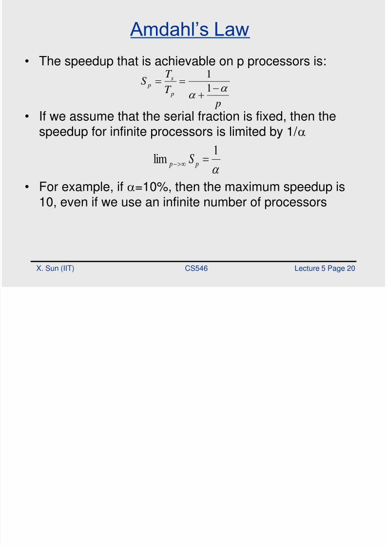
Amdahl’s Law
• The speedup that is achievable on p processors is:
• If we assume that the serial fraction is fixed, then the
speedup for infinite processors is limited by 1/
• For example, if =10%, then the maximum speedup is
10, even if we use an infinite number of processors
p
T
T S
p
s p
1
1
1lim p p S

8/2/2019 cs546perf
http://slidepdf.com/reader/full/cs546perf 21/78
X. Sun (IIT) CS546 Lecture 5 Page 21
Comments on Amdahl’s Law
• The Amdahl’s fraction in practice depends on the problem size
n and the number of processors p • An effective parallel algorithm has:
• For such a case, even if one fixes p , we can get linear speedups
by choosing a suitable large problem size
• Scalable speedup
• Practically, the problem size that we can run for a particularproblem is limited by the time and memory of the parallelcomputer
n pn as0),(
n p pn p
p
T
T S
p
s p as
),()1(1

8/2/2019 cs546perf
http://slidepdf.com/reader/full/cs546perf 22/78
X. Sun (IIT) CS546 Lecture 5 Page 22
• Fixed-Time Speedup (Gustafson, 88)
° Emphasis on work finished in a fixed time
° Problem size is scaled from W to W '
° W' : Work finished within the fixed time with parallel
processing
W
W
Solvingof TimeorUniprocess
'Solvingof TimeorUniprocess
'Solvingof TimeParallel
'Solvingof TimeorUniprocess'
W
W S p
W
W '

8/2/2019 cs546perf
http://slidepdf.com/reader/full/cs546perf 23/78
X. Sun (IIT) CS546 Lecture 5 Page 23
Gustafson’s Law (Without Overhead)
a 1-a time
p (1-a)p
ps
s
t t
t
pW
pW W Work
pWork SpeedupFT )1(1()1()(

8/2/2019 cs546perf
http://slidepdf.com/reader/full/cs546perf 24/78
X. Sun (IIT) CS546 Lecture 5 Page 24
• Fixed-Time Speedup (Gustafson)
Wp
W1 Wp
Wp
Wp Wp
W1
W1
W1
W1
1 2 3 4 5
Number of Processors (p)
Amount
of
Work
Tp
T1
Tp Tp Tp
T1 T1
Tp
T1 T1
1 2 3 4 5
Number of Processors (p)
Elapsed
Time

8/2/2019 cs546perf
http://slidepdf.com/reader/full/cs546perf 25/78
X. Sun (IIT) CS546 Lecture 5 Page 25
Converting ’s between Amdahl’s
and Gustafon’s laws
Based on this observation,
Amdahl’s and Gustafon’s laws
are identical.
p p
pGG
A)1(1)1(
G
G
A
p
).1(
1
1

8/2/2019 cs546perf
http://slidepdf.com/reader/full/cs546perf 26/78
X. Sun (IIT) CS546 Lecture 5 Page 27
Memory Constrained Scaling:
Sun and Ni’s Law • Scale the largest possible solution limited by
the memory space. Or, fix memory usage perprocessor – (ex) N-body problem
• Problem size is scaled from W to W*• W* is the work executed under memorylimitation of a parallel computer
• For simple profile, and G(n) is the increase of
parallel workload as the memory capacityincreases p times.)(* * M pGW

8/2/2019 cs546perf
http://slidepdf.com/reader/full/cs546perf 27/78
X. Sun (IIT) CS546 Lecture 5 Page 28
Sun & Ni’s Law
timein Increase
work in Increase
TimeWork
pTime pWork Speedup MB
)1( / )1(
)( / )(
p pG
pG
TimeWork
pTime pWork Speedup MB
/ )()1(
)()1(
)1( / )1(
)( / )(
a 1-a
p (1-a)G(p)
time

8/2/2019 cs546perf
http://slidepdf.com/reader/full/cs546perf 28/78
X. Sun (IIT) CS546 Lecture 5 Page 29
• Memory-Bounded Speedup (Sun & Ni, 90)
° Emphasis on work finished under current physical
limitation
° Problem size is scaled from W to W *
°
W *
: Work executed under memory limitation withparallel processing
*
**
Solvingof TimeParallel
Solvingof TimeorUniprocess
W
W S p
• X.H. Sun, and L. Ni , "Scalable Problems and Memory-Bounded Speedup,"
Journal of Parallel and Distributed Computing, Vol. 19, pp.27-37, Sept. 1993 (SC90).

8/2/2019 cs546perf
http://slidepdf.com/reader/full/cs546perf 29/78
X. Sun (IIT) CS546 Lecture 5 Page 30
• Memory-Boundary Speedup (Sun & Ni)
Wp
W1
Wp
Wp
Wp Wp
W1
W1
W1
W1
1 2 3 4 5
Number of Processors (p)
Amount
of
Work
Tp
T1
Tp Tp Tp
T1 T1
Tp
T1 T1
1 2 3 4 5
Number of Processors (p)
Elapsed
Time
– Work executed under memory limitation
– Hierarchical memory

8/2/2019 cs546perf
http://slidepdf.com/reader/full/cs546perf 30/78
X. Sun (IIT) CS546 Lecture 5 Page 31
Characteristics
• Connection to other scaling models – G(p) = 1, problem constrained scaling
– G(p) = p, time constrained scaling
• With overhead
• G(p) > p, can lead to large increase inexecution time
– (ex) 10K x 10K matrix factorization: 800MB, 1 hr in
uniprocessorwith 1024 processors, 320K x 320K matrix, 32 hrs

8/2/2019 cs546perf
http://slidepdf.com/reader/full/cs546perf 31/78
X. Sun (IIT) CS546 Lecture 5 Page 32
– ScalableMore accurate solution
Sufficient parallelism
Maintain efficiency
– Efficient in parallelcomputingLoad balance
Communication
– Mathematically
effectiveAdaptive
Accuracy
Why Scalable Computing

8/2/2019 cs546perf
http://slidepdf.com/reader/full/cs546perf 32/78
X. Sun (IIT) CS546 Lecture 5 Page 33
• Memory-Bounded Speedup
° Natural for domain decomposition based computing
° Show the potential of parallel processing (In gerneal,
computing requirement increases faster with problem
size than that of communication)
° Impacts extend to architecture design: trade-off of
memory size and computing speed

8/2/2019 cs546perf
http://slidepdf.com/reader/full/cs546perf 33/78
X. Sun (IIT) CS546 Lecture 5 Page 34
Why Scalable Computing (2)
• Appropriate for small machine
– Parallelism overheads begin to dominate benefitsfor larger machines
• Load imbalance
• Communication to computation ratio
– May even achieve slowdowns
– Does not reflect real usage, and inappropriate for
large machine• Can exaggerate benefits of improvements
Small Work

8/2/2019 cs546perf
http://slidepdf.com/reader/full/cs546perf 34/78
X. Sun (IIT) CS546 Lecture 5 Page 35
Why Scalable Computing (3)
• Appropriate for big machine
– Difficult to measure improvement
– May not fit for small machine
• Can’t run
• Thrashing to disk
• Working set doesn’t fit in cache
– Fits at some p , leading to superlinear speedup
Large Work

8/2/2019 cs546perf
http://slidepdf.com/reader/full/cs546perf 35/78
X. Sun (IIT) CS546 Lecture 5 Page 36
Demonstrating Scaling Problems
parallelism
overhead
superlinear
User want to scale problems as machines grow!
Small Ocean problem
On SGI Origin2000
Big equation solver problem
On SGI Origin2000

8/2/2019 cs546perf
http://slidepdf.com/reader/full/cs546perf 36/78
X. Sun (IIT) CS546 Lecture 5 Page 37
How to Scale
• Scaling a machine – Make a machine more powerful
– Machine size• <processor, memory, communication, I/O>
– Scaling a machine in parallel processing• Add more identical nodes
• Problem size – Input configuration
– data set size : the amount of storage required to
run it on a single processor – memory usage : the amount of memory used by
the program

8/2/2019 cs546perf
http://slidepdf.com/reader/full/cs546perf 37/78
X. Sun (IIT) CS546 Lecture 5 Page 38
Two Key Issues in Problem Scaling
• Under what constraints should the problembe scaled?
– Some properties must be fixed as the machinescales
• How should the problem be scaled? – Which parameters?
– How?

8/2/2019 cs546perf
http://slidepdf.com/reader/full/cs546perf 38/78
X. Sun (IIT) CS546 Lecture 5 Page 39
Constraints To Scale
• Two types of constraints – Problem-oriented
• Ex) Time
– Resource-oriented
• Ex) Memory
• Work to scale
– Metric-oriented
• Floating point operation, instructions
– User-oriented
• Easy to change but may difficult to compare
• Ex) particles, rows, transactions
• Difficult cross comparison

8/2/2019 cs546perf
http://slidepdf.com/reader/full/cs546perf 39/78
X. Sun (IIT) CS546 Lecture 5 Page 40
• Speedup
Time ExecutionParallel
Time Executionor UniprocessS p
SpeedSequential
SpeedParallel pS
Rethinking of Speedup
• Why it is called speedup but compare time
• Could we compare speed directly?
• Generalized speedup
• X.H. Sun, and J. Gustafson, "Toward A Better Parallel Performance Metric,"
Parallel Computing, Vol. 17, pp.1093-1109, Dec. 1991.

8/2/2019 cs546perf
http://slidepdf.com/reader/full/cs546perf 40/78
X. Sun (IIT) CS546 Lecture 5 Page 41

8/2/2019 cs546perf
http://slidepdf.com/reader/full/cs546perf 41/78
X. Sun (IIT) CS546 Lecture 5 Page 42
Compute : Problem
• Consider parallel algorithm for computing the value of
=3.1415…through the following numericalintegration
dx
x
π
1
0 2
1
421
4
x
8/2/2019 cs546perf
http://slidepdf.com/reader/full/cs546perf 42/78
X. Sun (IIT) CS546 Lecture 5 Page 43
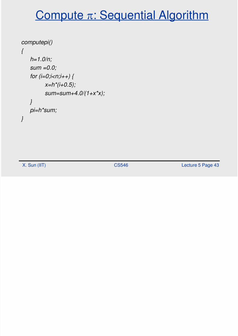
Compute : Sequential Algorithm
computepi(){
h=1.0/n;
sum =0.0;
for (i=0;i<n;i++) {
x=h*(i+0.5); sum=sum+4.0/(1+x*x);
}
pi=h*sum;
}
8/2/2019 cs546perf
http://slidepdf.com/reader/full/cs546perf 43/78
X. Sun (IIT) CS546 Lecture 5 Page 44
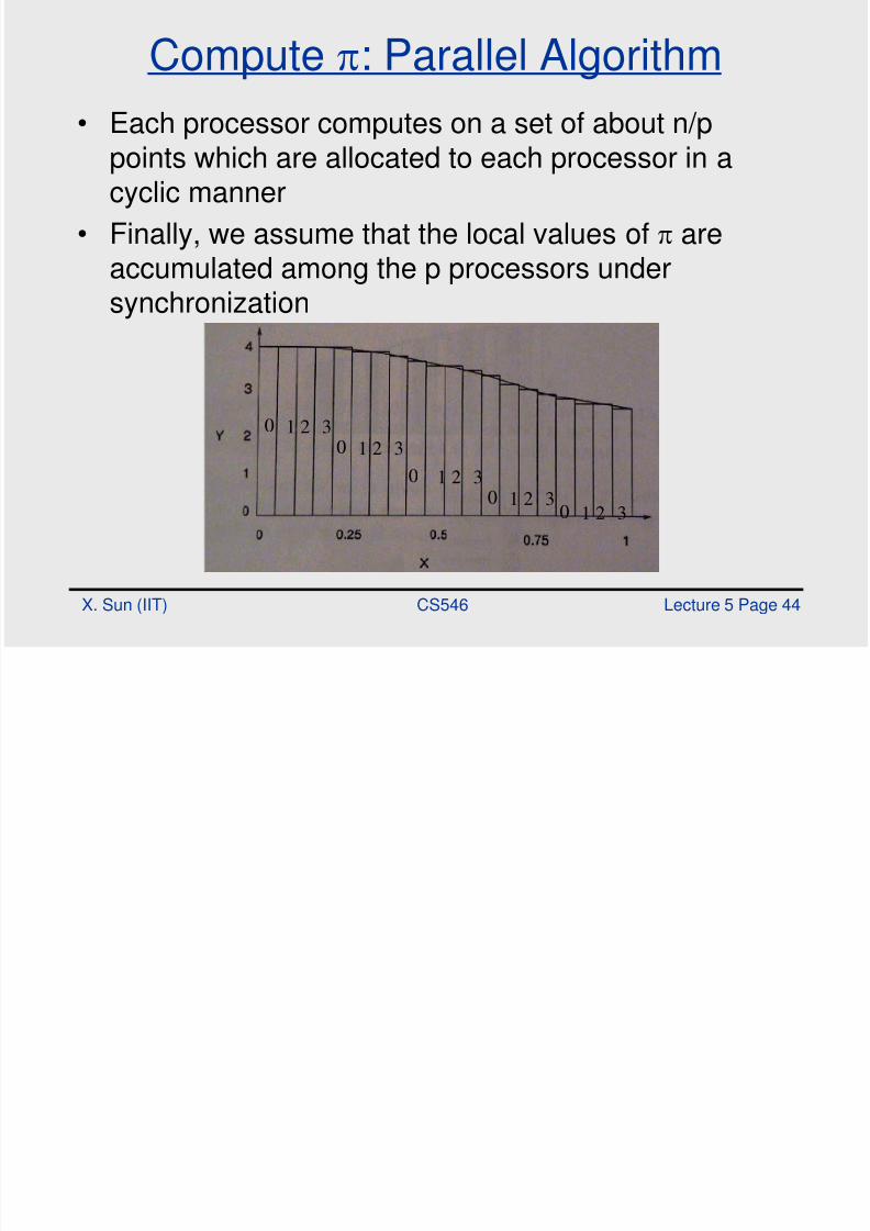
Compute : Parallel Algorithm
• Each processor computes on a set of about n/p
points which are allocated to each processor in acyclic manner
• Finally, we assume that the local values of areaccumulated among the p processors under
synchronization
01 2 3
01 2 3
01 2 3
01 2 3 0
1 2 3

8/2/2019 cs546perf
http://slidepdf.com/reader/full/cs546perf 44/78
X. Sun (IIT) CS546 Lecture 5 Page 45
Compute : Parallel Algorithm
computepi(){
id=my_proc_id();
nprocs=number_of_procs():
h=1.0/n;
sum=0.0;
for(i=id;i<n;i=i+nprocs) { x=h*(i+0.5);
sum=sum+4.0/(1+x*x);
}
localpi=sum*h;
use_tree_based_combining_for_critical_section();
pi=pi+localpi; end_critical_section();
}

8/2/2019 cs546perf
http://slidepdf.com/reader/full/cs546perf 45/78
X. Sun (IIT) CS546 Lecture 5 Page 46
Compute : Analysis
• Assume that the computation of is performed over n points
• The sequential algorithm performs 6 operations (twomultiplications, one division, three additions) per points on the x-axis. Hence, for n points, the number of operations executed in thesequential algorithm is:
nT s 6
for (i=0;i<n;i++) {
x=h*(i+0.5);
sum=sum+4.0/(1+x*x);
}
3 additions
2 multiplications
1 division

8/2/2019 cs546perf
http://slidepdf.com/reader/full/cs546perf 46/78
X. Sun (IIT) CS546 Lecture 5 Page 47
Compute : Analysis
• The parallel algorithm uses p processors with staticinterleaved scheduling. Each processor computes ona set of m points which are allocated to each processin a cyclic manner
• The expression for m is given by if p
does not exactly divide n. The runtime for the parallelalgorithm for the parallel computation of the localvalues of is:
1 p
nm
00 )66(*6 t p
nt mT p

8/2/2019 cs546perf
http://slidepdf.com/reader/full/cs546perf 47/78
X. Sun (IIT) CS546 Lecture 5 Page 48
Compute : Analysis
• The accumulation of the local values of
using atree-based combining can be optimally performed inlog2(p) steps
• The total runtime for the parallel algorithm for thecomputation of including the parallel computationand the combining is:
• The speedup of the parallel algorithm is:
))(log()66(*6 000 c p t t pt p
nt mT
) / 1)(log(66
6
0t t p p
nn
T T S
c p
s p
8/2/2019 cs546perf
http://slidepdf.com/reader/full/cs546perf 48/78
X. Sun (IIT) CS546 Lecture 5 Page 49
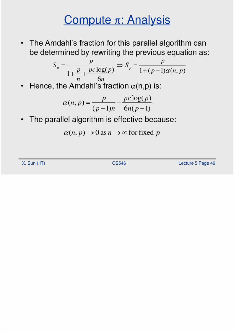
Compute : Analysis
• The Amdahl’s fraction for this parallel algorithm canbe determined by rewriting the previous equation as:
• Hence, the Amdahl’s fraction (n,p) is:
• The parallel algorithm is effective because:
),()1(1
6
)log(1
pn p
pS
n
p pc
n
p
pS p p
)1(6
)log(
)1(),(
pn
p pc
n p
p pn
pn pn fixedforas0),(

8/2/2019 cs546perf
http://slidepdf.com/reader/full/cs546perf 49/78
X. Sun (IIT) CS546 Lecture 5 Page 50
Finite Differences: Problem
• Consider a finite difference iterative method appliedto a 2D grid where:
t
ji
t
ji
t
ji
t
ji
t
ji
t
ji X X X X X X ,,1,11,1,
1
, )1()(

8/2/2019 cs546perf
http://slidepdf.com/reader/full/cs546perf 50/78
X. Sun (IIT) CS546 Lecture 5 Page 51
Finite Differences: Serial Algorithm
finitediff(){
for (t=0;t<T;t++) {
for (i=0;i<n;i++) {
for (j=0;j<n;j++) {
x[i,j]=w_1*(x[i,j-1]+x[i,j+1]+x[i-1,j]+x[i+1,j]+w_2*x[i,j]; }
}
}
}

8/2/2019 cs546perf
http://slidepdf.com/reader/full/cs546perf 51/78
X. Sun (IIT) CS546 Lecture 5 Page 52
Finite Differences: Parallel Algorithm
• Each processor computes on a sub-grid ofpoints
• Synch between processors after every iterationensures correct values being used for subsequent
iterations
p
n
p
n
p
n

8/2/2019 cs546perf
http://slidepdf.com/reader/full/cs546perf 52/78
X. Sun (IIT) CS546 Lecture 5 Page 53
Finite Differences: Parallel Algorithm
finitediff(){
row_id=my_processor_row_id();
col_id=my_processor_col_id();
p=numbre_of_processors();
sp=sqrt(p);
rows=cols=ceil(n/sp); row_start=row_id*rows;
col_start=col_id*cols;
for (t=0;t<T;t++) {
for (i=row_start;i<min(row_start+rows,n);i++) {
for (j=col_start;j<min(col_start+cols,n);j++) {
x[i,j]=w_1*(x[i,j-1]+x[i,j+1]+x[i-1,j]+x[i+1,j]+w_2*x[i,j]; }
barrier();
}
}
}

8/2/2019 cs546perf
http://slidepdf.com/reader/full/cs546perf 53/78
X. Sun (IIT) CS546 Lecture 5 Page 54
Finite Differences:Analysis
• The sequential algorithm performs 6 operations(2multiplications, 4 additions) every iteration per point on the grid.Hence, for an n*n grid and T iterations, the number of operationsexecuted in the sequential algorithm is:
0
2
6 t nT s
x[i,j]=w_1*(x[i,j-1]+x[i,j+1]+x[i-1,j]+x[i+1,j]+w_2*x[i,j];
2 multiplications
4 additions
8/2/2019 cs546perf
http://slidepdf.com/reader/full/cs546perf 54/78
X. Sun (IIT) CS546 Lecture 5 Page 55
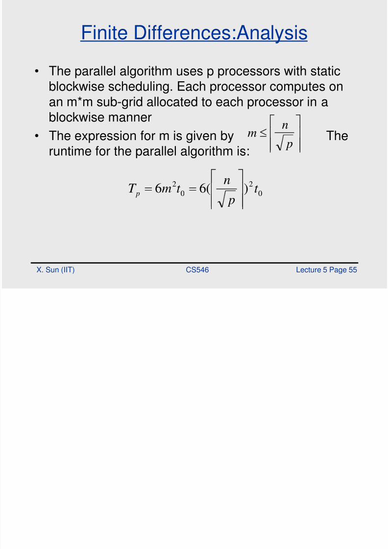
Finite Differences:Analysis
• The parallel algorithm uses p processors with staticblockwise scheduling. Each processor computes onan m*m sub-grid allocated to each processor in ablockwise manner
• The expression for m is given by Theruntime for the parallel algorithm is:
p
nm
0
2
0
2 )(66 t p
nt mT p

8/2/2019 cs546perf
http://slidepdf.com/reader/full/cs546perf 55/78
X. Sun (IIT) CS546 Lecture 5 Page 56
Finite Differences:Analysis
• The barrier synch needed for each iteration can be optimally
performed in log(p) steps
• The total runtime for the parallel algorithm for the computationis:
• The speedup of the parallel algorithm is:
))(log(6))(log()(66 00
2
00
2
0
2
cc p t t pt p
n
t t pt p
n
t mT
) / 1)(log(6
6
0
2
2
t t p p
nn
T T S
c p
s p

8/2/2019 cs546perf
http://slidepdf.com/reader/full/cs546perf 56/78
X. Sun (IIT) CS546 Lecture 5 Page 57
Finite Differences:Analysis
• The Amdahl’s fraction for this parallel algorithm can be
determined by rewriting the previous equation as:
• Hence, the Amdahl’s fraction (n.p) is:
• We finally note that
• Hence, the parallel algorithm is effective
),()1(1
6
)log(1
2
pn p
pS
n
p pc
pS p p
26)1(
)log(),(
n p
p pc pn
pfixedforas0),( n pn
E i S l

8/2/2019 cs546perf
http://slidepdf.com/reader/full/cs546perf 57/78
X. Sun (IIT) CS546 Lecture 5 Page 58
Equation Solver
A[i,j] = 0.2 * (A[i, j] + A[i, j-1] + A[i-1, j] + a[i, j+1] + a[i+1, j])
n
nprocedure solve (A)
…
while(!done) do
diff = 0;
for i = 1 to n do
for j = 1 to n do
temp = A[i, j];
A[i, j] = … diff += abs(A[i,j] – temp);
end for
end for
if (diff/(n*n) < TOL) then done =1 ;
end whileend procedure
W kl d

8/2/2019 cs546perf
http://slidepdf.com/reader/full/cs546perf 58/78
X. Sun (IIT) CS546 Lecture 5 Page 59
Workloads
• Basic properties – Memory requirement : O(n2)
– Computational complexity : O(n3), assuming the number ofiterations to converge to be O(n)
• Assume speedups equal to # of p
• Grid size – Fixed-size : fixed
– Fixed-time :
– Memory-bound :
n pk k pn 333
n pk k pn 22

8/2/2019 cs546perf
http://slidepdf.com/reader/full/cs546perf 59/78
X. Sun (IIT) CS546 Lecture 5 Page 60
Memory Requirement of Equation Solver
3
2232 )(
p
n
p
pn
p
k
Fixed-time: 33
k pn
Fixed-size :
Memory-bound : pn 2
,
p
n2

8/2/2019 cs546perf
http://slidepdf.com/reader/full/cs546perf 60/78
X. Sun (IIT) CS546 Lecture 5 Page 61
Time Complexity of Equation Solver
Fixed-time:
Fixed-size:
Memory-bound:
22k pn 33 )( pnk
Sequential time complexity
,
p
n3
3n
pn p
pn 33
)(

8/2/2019 cs546perf
http://slidepdf.com/reader/full/cs546perf 61/78
X. Sun (IIT) CS546 Lecture 5 Page 62
Concurrency
Fixed-time:
Fixed-size :
Memory-bound: 22 k pn
2
n
Concurrency is proportional to the number of grid points
33k pn 3 22232 )( pn pnk
,

8/2/2019 cs546perf
http://slidepdf.com/reader/full/cs546perf 62/78
X. Sun (IIT) CS546 Lecture 5 Page 63
Communication to Computation Ratio
n
p
p
n
p
n
p
n
CCR 22
2
1
Fixed-time :
Fixed-size : Memory-bound :
n p
p
pn
p
k
p
k p
k
CCR6
2322
2
)(11
n
p
pn
p
k
p
k
p
k
CCR1
)(
11
222
2
8/2/2019 cs546perf
http://slidepdf.com/reader/full/cs546perf 63/78
X. Sun (IIT) CS546 Lecture 5 Page 64
Scalability
• The Need for New Metrics
• Comparison of performances with different workload
• Availability of massively parallel processing
• Scalability
Ability to maintain parallel processing gain when both
problem size and system size increase

8/2/2019 cs546perf
http://slidepdf.com/reader/full/cs546perf 64/78
X. Sun (IIT) CS546 Lecture 5 Page 65
Parallel Efficiency
• The achieved fraction of total potential
parallel processing gain – Assuming linear speedup p is ideal case
• The ability to maintain efficiency whenproblem size increase
pS E p
p

8/2/2019 cs546perf
http://slidepdf.com/reader/full/cs546perf 65/78
X. Sun (IIT) CS546 Lecture 5 Page 66
Maintain Efficiency
• Efficiency of adding n numbers in parallel
– For an efficiency of 0.80 on 4 procs, n=64
– For an efficiency of 0.80 on 8 procs, n=192
– For an efficiency of 0.80 on 16 procs, n=512
Efficiency for Various Data Sizes
0
0.2
0.4
0.6
0.8
1
1 4 8 16 32
number of processors
E f f i c i e n c y
n=64
n=192
n=320
n=512
E=1/(1+2plogp/n)

8/2/2019 cs546perf
http://slidepdf.com/reader/full/cs546perf 66/78
X. Sun (IIT) CS546 Lecture 5 Page 67
• Ideally Scalable
T (m p, m W ) = T ( p, W )
– T: execution time
– W: work executed
– P: number of processors used
– m: scale up m times – work: flop count based on the best practical
serial algorithm
• Fact:
T (m
p, m
W ) = T ( p, W )if and only if
The Average Unit Speed Is Fixed

8/2/2019 cs546perf
http://slidepdf.com/reader/full/cs546perf 67/78
X. Sun (IIT) CS546 Lecture 5 Page 68
– Definition:
The average unit speed is the achieved speed divided by
the number of processors
– Definition (Isospeed Scalability):An algorithm-machine combination is scalable if the
achieved average unit speed can remain constant with
increasing numbers of processors, provided the problem
size is increased proportionally

8/2/2019 cs546perf
http://slidepdf.com/reader/full/cs546perf 68/78
X. Sun (IIT) CS546 Lecture 5 Page 69
• Isospeed Scalability (Sun & Rover, 91)
– W: work executed when p processors are employed
– W': work executed when p' > p processors are employed
to maintain the average speed
– Ideal case
– Scalability in terms of time
'
')',(
W p
W p p p yScalabilit
,'
' p
W pW
processors'on'work withtime
processorsonwork withtime
'',
' pW
pW
W T
W T p p
p
p
1)',( p p
8/2/2019 cs546perf
http://slidepdf.com/reader/full/cs546perf 69/78
X. Sun (IIT) CS546 Lecture 5 Page 70
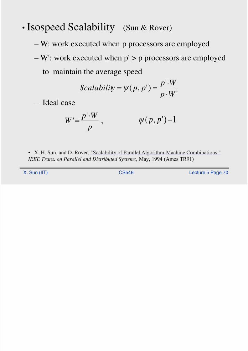
• Isospeed Scalability (Sun & Rover)
– W: work executed when p processors are employed – W': work executed when p' > p processors are employed
to maintain the average speed
– Ideal case'
'
)',( W p
W p
p p yScalabilit
,'
' p
W pW
1)',( p p
• X. H. Sun, and D. Rover, "Scalability of Parallel Algorithm-Machine Combinations,"
IEEE Trans. on Parallel and Distributed Systems, May, 1994 (Ames TR91)

8/2/2019 cs546perf
http://slidepdf.com/reader/full/cs546perf 70/78
X. Sun (IIT) CS546 Lecture 5 Page 71
The Relation of Scalability and Time
• More scalable leads to smaller time – Better initial run-time and higher scalability lead to
superior run-time
– Same initial run-time and same scalability lead to
same scaled performance – Superior initial performance may not last long if
scalability is low
• Range Comparison
• X.H. Sun, "Scalability Versus Execution Time in Scalable Systems,"
Journal of Parallel and Distributed Computing, Vol. 62, No. 2, pp. 173-192, Feb 2002.
Range Comparison Via Performance Crossing Point

8/2/2019 cs546perf
http://slidepdf.com/reader/full/cs546perf 71/78
X. Sun (IIT) CS546 Lecture 5 Page 72
Range Comparison Via Performance Crossing Point
Assume Program I is oz times slower than program 2 at the initial state
Begin (Range Comparison)
p' = p;
Repeat
p' = p' + 1;
Compute the scalability of program 1 (p,p');
Compute the scalability of program 2 (p,p') ;
Until ( (p,p') > (p,p') or p' = the limit of ensemble size)
If (p,p') > (p,p') Then
p is the smallest scaled crossing point;
program 2 is superior at any ensemble size p†, p p† < p'
Else program 2 is superior at any ensemble size p†, p p† p’
End {if}
End {Range Comparison}

8/2/2019 cs546perf
http://slidepdf.com/reader/full/cs546perf 72/78
X. Sun (IIT) CS546 Lecture 5 Page 73
• Range Comparison
Influence of Communication Speed Influence of Computing Speed
• X.H. Sun, M. Pantano, and Thomas Fahringer, "Integrated Range Comparison for Data-Parallel
Compilation Systems," IEEE Trans. on Parallel and Distributed Processing, May 1999.

8/2/2019 cs546perf
http://slidepdf.com/reader/full/cs546perf 73/78
X. Sun (IIT) CS546 Lecture 5 Page 74
The SCALA (SCALability Analyzer) System
• Design Goals
– Predict performance
– Support program optimization
– Estimate the influence of hardware variations• Uniqueness
– Designed to be integrated into advanced compilersystems
– Based on scalability analysis

8/2/2019 cs546perf
http://slidepdf.com/reader/full/cs546perf 74/78
X. Sun (IIT) CS546 Lecture 5 Page 75
• Vienna Fortran Compilation System
– A data-parallel restructuring compilation system
– Consists of a parallelizing compiler for VF/HPFand tools for program analysis and restructuring
– Under a major upgrade for HPF2
• Performance prediction is crucial forappropriate program restructuring

8/2/2019 cs546perf
http://slidepdf.com/reader/full/cs546perf 75/78
X. Sun (IIT) CS546 Lecture 5 Page 76
The Structure of SCALA

8/2/2019 cs546perf
http://slidepdf.com/reader/full/cs546perf 76/78
X. Sun (IIT) CS546 Lecture 5 Page 77
Prototype Implementation • Automatic range comparison for different data distributions
• The P 3 T static performance estimator
• Test cases: Jacobi and Redblack
No Crossing Point Have Crossing Point
Summary

8/2/2019 cs546perf
http://slidepdf.com/reader/full/cs546perf 77/78
X. Sun (IIT) CS546 Lecture 5 Page 78
Summary
• Relation between Iso-speed scalability and iso-efficiency scalability – Both measure the ability to maintain parallel efficiency
defined as
– Where iso-efficiency’s speedup is the traditional speedupdefined as
– Iso-speed’s speedup is the generalized speedup defined as
– If the the sequential execution speed is independent ofproblem size, iso-speed and iso-efficiency is equivalent
– Due to memory hierarchy, sequential execution performancevaries largely with problem size
p
S E
p
p
SpeedSequential
SpeedParallel pS
TimeExecutionParallelTimeExecutionorUniprocess pS

8/2/2019 cs546perf
http://slidepdf.com/reader/full/cs546perf 78/78
Summary
• Predict the sequential execution performancebecomes a major task of SCALA due to advancedmemory hierarchy
– Memory-LogP model is introduced for data access cost
• New challenge in distributed computing• Generalized iso-speed scalability
• Generalized performance tool: GHS
• K. Cameron and X.-H. Sun, "Quantifying Locality Effect in Data Access Delay: Memory logP,"
Proc. of 2003 IEEE IPDPS 2003, Nice, France, April, 2003.
• X.-H. Sun and M. Wu, "Grid Harvest Service: A System for Long-Term, Application-Level Task
Scheduling," Proc. of 2003 IEEE IPDPS 2003, Nice, France, April, 2003.