CS453 Lecture 3. A sequential algorithm is evaluated by its runtime (in general, asymptotic runtime as a function of input size). The asymptotic runtime.

Performance measuresCS453

Lecture 3

A sequential algorithm is evaluated by its runtime (in general, asymptotic runtime as a function of input size).

The asymptotic runtime of a sequential program is identical on any serial platform.

The parallel runtime of a program depends on the input size, the number of processors, and the communication parameters of the machine.

An algorithm must therefore be analyzed in the context of the underlying platform.

A parallel system is a combination of a parallel algorithm and an underlying platform.

Analytical Modeling - Basics

Ananth Grama, Purdue University, W. Lafayette

A number of performance measures are intuitive.

Wall clock time - the time from the start of the first processor to the stopping time of the last processor in a parallel assembly. But how does this scale when the number of processors is changed of the program is ported to another machine altogether?

How much faster is the parallel version? This requests the obvious follow-up question – what is the baseline serial version with which we compare? Can we use a suboptimal serial program to make our parallel program look faster?

Analytical Modeling - Basics


Sources of Overhead in Parallel Programs If I use two processors, shouldn't my program run twice as fast?

No - a number of overheads, including wasted computation, communication, idling, and contention cause degradation in performance.

The execution profile of a hypothetical parallel program executing on eight processing elements. Profile indicates times spent performing computation (both essential and excess), communication, and idling.


Inter-process interactions: Processors working on any non-trivial parallel problem will need to talk to each other.

Idling: Processes may idle because of load imbalance, synchronization, or serial components.

Excess Computation: This is computation not performed by the serial version. This might be because the serial algorithm is difficult to parallelize, or that some computations are repeated across processors to minimize communication.

Sources of Overheads in Parallel Programs


Serial runtime of a program is the time elapsed between the beginning and the end of its execution on a sequential computer.

The parallel runtime is the time that elapses from the moment the first processor starts to the moment the last processor finishes execution.

We denote the serial runtime by Ts and the parallel runtime by TP .

Performance Metrics for Parallel Systems: Execution Time


Let Tall be the total time collectively spent by all the processing elements.

TS is the serial time. Observe that Tall - TS is then the total time

spend by all processors combined in non-useful work. This is called the total overhead.

The total time collectively spent by all the processing elements Tall = p TP (p is the number of processors).

The overhead function (To) is therefore given by

To = p TP - TS

Performance Metrics for Parallel Systems: Total Parallel Overhead


What is the benefit from parallelism?

Speedup (S) is the ratio of the time taken to solve a problem on a single processor to the time required to solve the same problem on a parallel computer with p identical processing elements.

Performance Metrics for Parallel Systems: Speedup


Consider the problem of adding n numbers by using n processing elements.

If n is a power of two, we can perform this operation in log n steps by propagating partial sums up a logical binary tree of processors.

Performance Metrics: Example


Performance Metrics: Example

Computing the global sum of 16 partial sums using 16 processing elements . Σj

i denotes the sum of numbers with consecutive labels from i to j .

Ananth Grama, Purdue University, W. LafayetteAnanth Grama, Purdue University, W. Lafayette

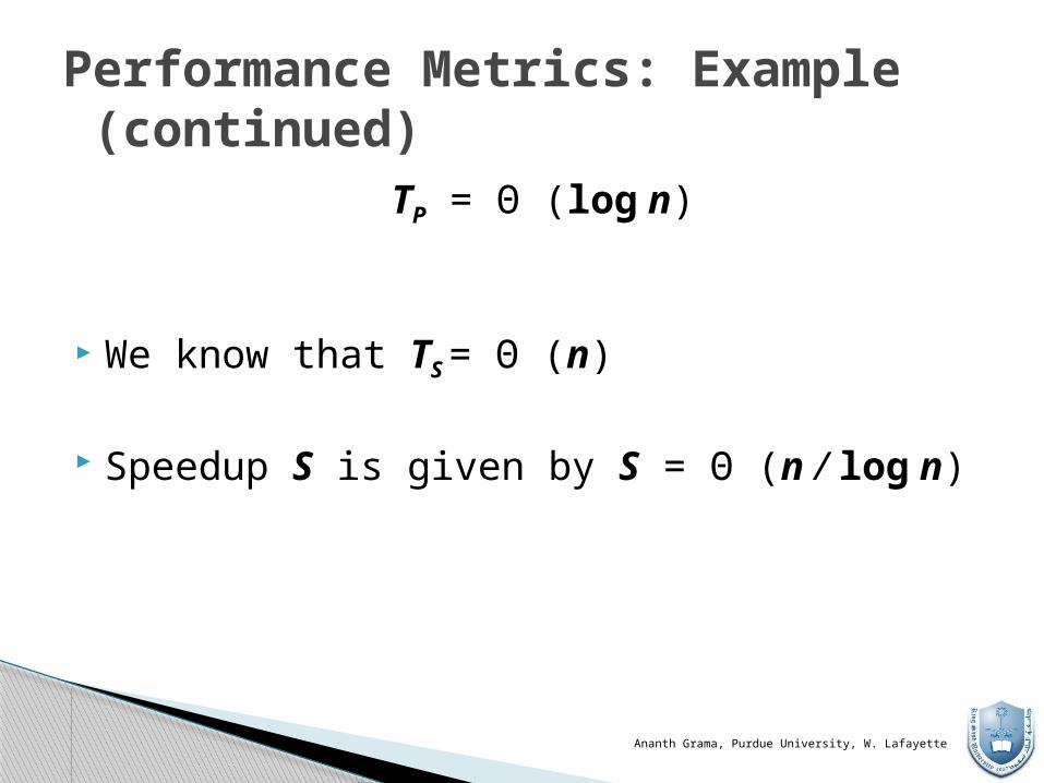
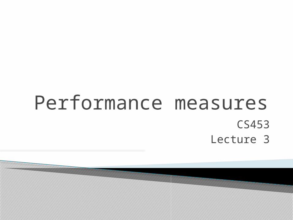
TP = Θ (log n)

We know that TS = Θ (n)

Speedup S is given by S = Θ (n / log n)

Performance Metrics: Example (continued)


For a given problem, there might be many serial algorithms available. These algorithms may have different asymptotic runtimes and may be parallelizable to different degrees.

For the purpose of computing speedup, we always consider the best sequential program as the baseline.

Performance Metrics: Speedup


Consider the problem of parallel bubble sort.

The serial time for bubblesort is 150 seconds.

The parallel time for odd-even sort (efficient parallelization of bubble sort) is 40 seconds.

The speedup would appear to be 150/40 = 3.75.

But is this really a fair assessment of the system?

What if serial quicksort only took 30 seconds? In this case, the speedup is 30/40 = 0.75. This is a more realistic assessment of the system.

Performance Metrics: Speedup Example


Speedup can be as low as 0 (the parallel program never terminates).

Speedup, in theory, should be upper bounded by p - after all, we can only expect a p-fold speedup if we use times as many resources.

A speedup greater than p is possible only if each processing element spends less than time TS / p solving the problem.

In this case, a single processor could be time slided to achieve a faster serial program, which contradicts our assumption of fastest serial program as basis for speedup.

Performance Metrics: Speedup Bounds


Performance Metrics: Efficiency Efficiency is a measure of the fraction of

time for which a processing element is usefully employed

Mathematically, it is given by

=

Following the bounds on speedup, efficiency can be as low as 0 and as high as 1.


Performance Metrics: Efficiency Example The speedup of adding numbers on processors is

given by

Efficiency is given by

=

=


Cost is the product of parallel runtime and the number of processing elements used (p x TP ).

Cost reflects the sum of the time that each processing element spends solving the problem.

A parallel system is said to be cost-optimal if the cost of solving a problem on a parallel computer is asymptotically identical to serial cost.

Since E = TS / p TP, for cost optimal systems, E = O(1).

Cost is sometimes referred to as work or processor-time product.

Cost of a Parallel System


Consider the problem of adding numbers on processors.

We have, TP = log n (for p = n).

The cost of this system is given by p TP = n log n.

Since the serial runtime of this operation is Θ(n), the algorithm is not cost optimal.

Cost of a Parallel System: Example


Consider a sorting algorithm that uses n processing elements to sort the list in time (log n)2.

Since the serial runtime of a (comparison-based) sort is n log n, the speedup and efficiency of this algorithm are given by n / log n and 1 / log n, respectively.

The p TP product of this algorithm is n (log n)2.

This algorithm is not cost optimal but only by a factor of log n.

If p < n, assigning n tasks to p processors gives TP = n (log n)2 / p .

The corresponding speedup of this formulation is p / log n.

This speedup goes down as the problem size n is increased for a given p !

Impact of Non-Cost Optimality


Often, using fewer processors improves performance of parallel systems.

Using fewer than the maximum possible number of processing elements to execute a parallel algorithm is called scaling down a parallel system.

A naive way of scaling down is to think of each processor in the original case as a virtual processor and to assign virtual processors equally to scaled down processors.

Since the number of processing elements decreases by a factor of n / p, the computation at each processing element increases by a factor of n / p.

The communication cost should not increase by this factor since some of the virtual processors assigned to a physical processors might talk to each other. This is the basic reason for the improvement from building granularity.

Effect of Granularity on Performance


Consider the problem of adding n numbers on p processing elements such that p < n and both n and p are powers of 2.

Use the parallel algorithm for n processors, except, in this case, we think of them as virtual processors.

Each of the p processors is now assigned n / p virtual processors.

The first log p of the log n steps of the original algorithm are simulated in (n / p) log p steps on p processing elements.

Subsequent log n - log p steps do not require any communication.

Building Granularity: Example


The overall parallel execution time of this parallel system is Θ ( (n / p) log p).

The cost is Θ (n log p), which is asymptotically higher than the Θ (n) cost of adding n numbers sequentially. Therefore, the parallel system is not cost-optimal.

Building Granularity: Example (continued)


CS453 Lecture 3. A sequential algorithm is evaluated by its runtime (in general, asymptotic runtime as a function of input size). The asymptotic runtime.

Documents