CS267 L23 Load Balancing and Scheduling.1 Demmel Sp 1999 CS 267 Applications of Parallel Computers Lecture 23: Load Balancing and Scheduling James Demmel http://www.cs.berkeley.edu/~demmel/ cs267_Spr99

CS267 L23 Load Balancing and Scheduling.1 Demmel Sp 1999 CS 267 Applications of Parallel Computers Lecture 23: Load Balancing and Scheduling James Demmel.
Dec 20, 2015
Welcome message from author
This document is posted to help you gain knowledge. Please leave a comment to let me know what you think about it! Share it to your friends and learn new things together.
Transcript

CS267 L23 Load Balancing and Scheduling.1 Demmel Sp 1999
CS 267 Applications of Parallel Computers
Lecture 23:
Load Balancing and Scheduling
James Demmel
http://www.cs.berkeley.edu/~demmel/cs267_Spr99

CS267 L23 Load Balancing and Scheduling.2 Demmel Sp 1999
Outline° Recall graph partitioning as load balancing technique
° Overview of load balancing problems, as determined by• Task costs
• Task dependencies
• Locality needs
° Spectrum of solutions• Static - all information available before starting
• Semi-Static - some info before starting
• Dynamic - little or no info before starting
° Survey of solutions• How each one works
• Theoretical bounds, if any
• When to use it

CS267 L23 Load Balancing and Scheduling.3 Demmel Sp 1999
Review of Graph Partitioning° Partition G(N,E) so that
• N = N1 U … U Np, with each |Ni| ~ |N|/p
• As few edges connecting different Ni and Nk as possible
° If N = {tasks}, each unit cost, edge e=(i,j) means task i has to communicate with task j, then partitioning means• balancing the load, i.e. each |Ni| ~ |N|/p
• minimizing communication
° Optimal graph partitioning is NP complete, so we use heuristics (see Lectures 14 and 15)• Spectral
• Kernighan-Lin
• Multilevel
° Speed of partitioner trades off with quality of partition• Better load balance costs more; may or may not be worth it

CS267 L23 Load Balancing and Scheduling.4 Demmel Sp 1999
Load Balancing in General
Enormous and diverse literature on load balancing
° Computer Science systems • operating systems
• parallel computing
• distributed computing
° Computer Science theory
° Operations research (IEOR)
° Application domains
A closely related problem is scheduling, which is to determine the order in which tasks run

CS267 L23 Load Balancing and Scheduling.5 Demmel Sp 1999
Understanding Different Load Balancing Problems
Load balancing problems differ in:
° Tasks costs• Do all tasks have equal costs?
• If not, when are the costs known?- Before starting, when task created, or only when task ends
° Task dependencies• Can all tasks be run in any order (including parallel)?
• If not, when are the dependencies known?- Before starting, when task created, or only when task ends
° Locality• Is it important for some tasks to be scheduled on the same
processor (or nearby) to reduce communication cost?
• When is the information about communication between tasks known?

CS267 L23 Load Balancing and Scheduling.6 Demmel Sp 1999
Task cost spectrum

CS267 L23 Load Balancing and Scheduling.7 Demmel Sp 1999
Task Dependency Spectrum
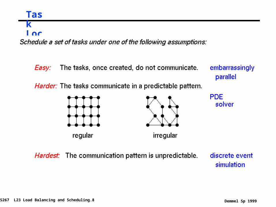
CS267 L23 Load Balancing and Scheduling.8 Demmel Sp 1999
Task Locality Spectrum (Data Dependencies)

CS267 L23 Load Balancing and Scheduling.9 Demmel Sp 1999
Spectrum of Solutions
One of the key questions is when certain information about the load balancing problem is known
Leads to a spectrum of solutions:
° Static scheduling. All information is available to scheduling algorithm, which runs before any real computation starts. (offline algorithms)
° Semi-static scheduling. Information may be known at program startup, or the beginning of each timestep, or at other well-defined points. Offline algorithms may be used even though the problem is dynamic.
° Dynamic scheduling. Information is not known until mid-execution. (online algorithms)

CS267 L23 Load Balancing and Scheduling.10 Demmel Sp 1999
Approaches
° Static load balancing
° Semi-static load balancing
° Self-scheduling
° Distributed task queues
° Diffusion-based load balancing
° DAG scheduling
° Mixed Parallelism
Note: these are not all-inclusive, but represent some of the problems for which good solutions exist.

CS267 L23 Load Balancing and Scheduling.11 Demmel Sp 1999
Static Load Balancing
° Static load balancing is use when all information is available in advance
° Common cases:• dense matrix algorithms, such as LU factorization
- done using blocked/cyclic layout
- blocked for locality, cyclic for load balance
• most computations on a regular mesh, e.g., FFT
- done using cyclic+transpose+blocked layout for 1D
- similar for higher dimensions, i.e., with transpose
• sparse-matrix-vector multiplication
- use graph partitioning
- assumes graph does not change over time (or at least within a timestep during iterative solve)

CS267 L23 Load Balancing and Scheduling.12 Demmel Sp 1999
Semi-Static Load Balance
° If domain changes slowly over time and locality is important• use static algorithm
• do some computation (usually one or more timesteps) allowing some load imbalance on later steps
• recompute a new load balance using static algorithm
° Often used in:• particle simulations, particle-in-cell (PIC) methods
- poor locality may be more of a problem than load imbalance as particles move from one grid partition to another
• tree-structured computations (Barnes Hut, etc.)
• grid computations with dynamically changing grid, which changes slowly

CS267 L23 Load Balancing and Scheduling.13 Demmel Sp 1999
Self-Scheduling° Self scheduling:• Keep a centralized pool of tasks that are available to run
• When a processor completes its current task, look at the pool
• If the computation of one task generates more, add them to the pool
° Originally used for:• Scheduling loops by compiler (really the runtime-system)
• Original paper by Tang and Yew, ICPP 1986
CS267 L23 Load Balancing and Scheduling.14 Demmel Sp 1999
When is Self-Scheduling a Good Idea?
Useful when:
° A batch (or set) of tasks without dependencies• can also be used with dependencies, but most analysis has only
been done for task sets without dependencies
° The cost of each task is unknown
° Locality is not important
° Using a shared memory multiprocessor, so a centralized pool of tasks is fine

CS267 L23 Load Balancing and Scheduling.15 Demmel Sp 1999
Variations on Self-Scheduling
° Typically, don’t want to grab smallest unit of parallel work.
° Instead, choose a chunk of tasks of size K.• If K is large, access overhead for task queue is small
• If K is small, we are likely to have even finish times (load balance)
° Four variations:• Use a fixed chunk size
• Guided self-scheduling
• Tapering
• Weighted Factoring
• Note: there are more

CS267 L23 Load Balancing and Scheduling.16 Demmel Sp 1999
Variation 1: Fixed Chunk Size° Kruskal and Weiss give a technique for computing
the optimal chunk size
° Requires a lot of information about the problem characteristics• e.g., task costs, number
° Results in an off-line algorithm. Not very useful in practice. • For use in a compiler, for example, the compiler would have to
estimate the cost of each task
• All tasks must be known in advance
CS267 L23 Load Balancing and Scheduling.17 Demmel Sp 1999
Variation 2: Guided Self-Scheduling
° Idea: use larger chunks at the beginning to avoid excessive overhead and smaller chunks near the end to even out the finish times.
° The chunk size Ki at the ith access to the task pool is given by
ceiling(Ri/p)
° where Ri is the total number of tasks remaining and
° p is the number of processors
° See Polychronopolous, “Guided Self-Scheduling: A Practical Scheduling Scheme for Parallel Supercomputers,” IEEE Transactions on Computers, Dec. 1987.

CS267 L23 Load Balancing and Scheduling.18 Demmel Sp 1999
Variation 3: Tapering
° Idea: the chunk size, Ki is a function of not only the remaining work, but also the task cost variance• variance is estimated using history information
• high variance => small chunk size should be used
• low variant => larger chunks OK
° See S. Lucco, “Adaptive Parallel Programs,” PhD Thesis, UCB, CSD-95-864, 1994.• Gives analysis (based on workload distribution)
• Also gives experimental results -- tapering always works at least as well as GSS, although difference is often small

CS267 L23 Load Balancing and Scheduling.19 Demmel Sp 1999
Variation 4: Weighted Factoring
° Idea: similar to self-scheduling, but divide task cost by computational power of requesting node
° Useful for heterogeneous systems
° Also useful for shared resource NOWs, e.g., built using all the machines in a building• as with Tapering, historical information is used to predict future
speed
• “speed” may depend on the other loads currently on a given processor
° See Hummel, Schmit, Uma, and Wein, SPAA ‘96• includes experimental data and analysis

CS267 L23 Load Balancing and Scheduling.20 Demmel Sp 1999
Distributed Task Queues
° The obvious extension of self-scheduling to distributed memory is:• a distributed task queue (or bag)
° When are these a good idea?• Distributed memory multiprocessors
• Or, shared memory with significant synchronization overhead
• Locality is not (very) important
• Tasks that are:
- known in advance, e.g., a bag of independent ones
- dependencies exist, i.e., being computed on the fly
• The costs of tasks is not known in advance

CS267 L23 Load Balancing and Scheduling.21 Demmel Sp 1999
Theoretical Results
Main result: A simple randomized algorithm is optimal with high probability
° Adler et al [95] show this for independent, equal sized tasks• “throw balls into random bins”
• tight bounds on load imbalance; show p log p tasks leads to “good” balance
° Karp and Zhang [88] show this for a tree of unit cost (equal size) tasks • parent must be done before children, tree unfolds at runtime
• children “pushed” to random processors
° Blumofe and Leiserson [94] show this for a fixed task tree of variable cost tasks
• their algorithm uses task pulling (stealing) instead of pushing, which is good for locality
• I.e., when a processor becomes idle, it steals from a random processor
• also have (loose) bounds on the total memory required
° Chakrabarti et al [94] show this for a dynamic tree of variable cost tasks• works for branch and bound, I.e. tree structure can depend on execution order
• uses randomized pushing of tasks instead of pulling, so worse locality
° Open problem: does task pulling provably work well for dynamic trees?

CS267 L23 Load Balancing and Scheduling.22 Demmel Sp 1999
Engineering Distributed Task Queues
A lot of papers on engineering these systems on various machines, and their applications
° If nothing is known about task costs when created• organize local tasks as a stack (push/pop from top)
• steal from the stack bottom (as if it were a queue), because old tasks likely to cost more
° If something is known about tasks costs and communication costs, can be used as hints. (See Wen, UCB PhD, 1996.)• Part of Multipol (www.cs.berkeley.edu/projects/multipol)
• Try to push tasks with high ratio of cost to compute/cost to push
- Ex: for matmul, ratio = 2n3 cost(flop) / 2n2 cost(send a word)
° Goldstein, Rogers, Grunwald, and others (independent work) have all shown • advantages of integrating into the language framework
• very lightweight thread creation
° CILK (Leicerson et al) (supertech.lcs.mit.edu/cilk)

CS267 L23 Load Balancing and Scheduling.23 Demmel Sp 1999
Diffusion-Based Load Balancing
° In the randomized schemes, the machine is treated as fully-connected.
° Diffusion-based load balancing takes topology into account• Locality properties better than prior work
• Load balancing somewhat slower than randomized
• Cost of tasks must be known at creation time
• No dependencies between tasks
CS267 L23 Load Balancing and Scheduling.24 Demmel Sp 1999
Diffusion-based load balancing° The machine is modeled as a graph
° At each step, we compute the weight of task remaining on each processor• This is simply the number if they are unit cost tasks
° Each processor compares its weight with its neighbors and performs some averaging• Markov chain analysis
° See Ghosh et al, SPAA96 for a second order diffusive load balancing algorithm• takes into account amount of work sent last time
• avoids some oscillation of first order schemes
° Note: locality is still not a major concern, although balancing with neighbors may be better than random

CS267 L23 Load Balancing and Scheduling.25 Demmel Sp 1999
DAG Scheduling
° For some problems, you have a directed acyclic graph (DAG) of tasks• nodes represent computation (may be weighted)
• edges represent orderings and usually communication (may also be weighted)
• not that common to have the DAG in advance
° Two application domains where DAGs are known• Digital Signal Processing computations
• Sparse direct solvers (mainly Cholesky, since it doesn’t require pivoting). More on this in another lecture.
° The basic offline strategy: partition DAG to minimize communication and keep all processors busy• NP complete, so need approximations
• Different than graph partitioning, which was for tasks with communication but no dependencies
• See Gerasoulis and Yang, IEEE Transaction on P&DS, Jun ‘93.
CS267 L23 Load Balancing and Scheduling.26 Demmel Sp 1999
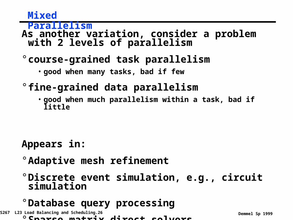
Mixed Parallelism
As another variation, consider a problem with 2 levels of parallelism
° course-grained task parallelism• good when many tasks, bad if few
° fine-grained data parallelism• good when much parallelism within a task, bad if little
Appears in:
° Adaptive mesh refinement
° Discrete event simulation, e.g., circuit simulation
° Database query processing
° Sparse matrix direct solvers
CS267 L23 Load Balancing and Scheduling.27 Demmel Sp 1999
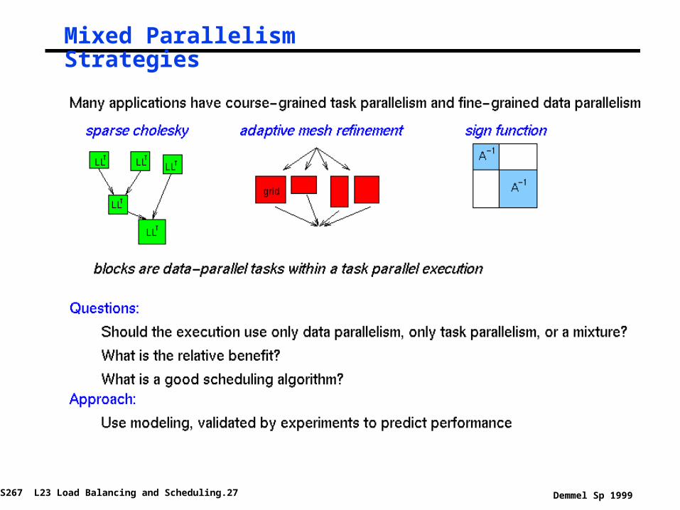
Mixed Parallelism Strategies

CS267 L23 Load Balancing and Scheduling.28 Demmel Sp 1999
Which Strategy to Use

CS267 L23 Load Balancing and Scheduling.29 Demmel Sp 1999
Switch Parallelism: A Special Case
CS267 L23 Load Balancing and Scheduling.30 Demmel Sp 1999
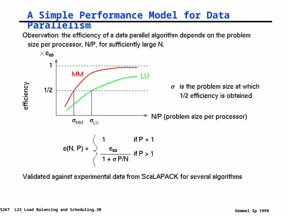
A Simple Performance Model for Data Parallelism
CS267 L23 Load Balancing and Scheduling.31 Demmel Sp 1999

CS267 L23 Load Balancing and Scheduling.32 Demmel Sp 1999
Values of Sigma (Problem Size for Half Peak)

CS267 L23 Load Balancing and Scheduling.33 Demmel Sp 1999
Modeling performance° To predict performance, make assumptions about
task tree• complete tree with branching factor d>= 2
• d child tasks of parent of size N are all of size N/c, c>1
• work to do task of size N is O(Na), a>= 1
° Example: Sign function based eigenvalue routine• d=2, c=4 (on average), a=1.5
° Example: Sparse Cholesky on 2D mesh• d=4, c=4, a=1.5
° Combine these assumptions with model of data parallelism

CS267 L23 Load Balancing and Scheduling.34 Demmel Sp 1999
Simulated efficiency of Sign Function Eigensolver• Starred lines are optimal mixed parallelism• Solid lines are data parallelism• Dashed lines are switched parallelism

CS267 L23 Load Balancing and Scheduling.35 Demmel Sp 1999
Simulated efficiency of Sparse Cholesky• Starred lines are optimal mixed parallelism• Solid lines are data parallelism• Dashed lines are switched parallelism

CS267 L23 Load Balancing and Scheduling.36 Demmel Sp 1999
Actual Speed of Sign Function Eigensolver• Starred lines are optimal mixed parallelism• Solid lines are data parallelism• Dashed lines are switched parallelism• Intel Paragon, built on ScaLAPACK• Switched parallelism worthwhile!
Related Documents