CS Example: General Linear Test (cs2.sas) proc reg data=cs; model gpa=satm satv hsm hss hse; * test H0: beta1 = beta2 = 0; sat: test satm, satv; * test.

CS Example: General Linear Test (cs2.sas)

proc reg data=cs; model gpa=satm satv hsm hss hse; * test H0: beta1 = beta2 = 0; sat: test satm, satv; * test H0: beta3=beta4=beta5=0; hs: test hsm, hss, hse;run;

CS Example: General Linear TestTest sat Results for Dependent Variable gpa

Source DF MeanSquare

F Value Pr > F

Numerator 2 0.46566 0.95 0.3882

Denominator 218 0.49000

Test hs Results for Dependent Variable gpa


F Value Pr > F

Numerator 3 6.68660 13.65 <.0001


CS Example: General Linear Test

proc reg data=cs; model gpa=satm hsm hss hse; * test H0: beta1 = beta2 = 0; sat: test satm; * test H0: beta3=beta4=beta5=0; hs: test hsm, hss, hse;run;

Body Fat Example (nknw260.sas)

For 20 healthy female subjects between 25 – 30

Y = amount of body fat (fat)

X1 = tricepts skinfold thickness (skinfold)

X2 = thigh circumference (thigh)

X3 = midarm circumference (midarm)

Body Fat Example: Regression (input)

data bodyfat; infile 'I:\My Documents\Stat 512\CH07TA01.DAT'; input skinfold thigh midarm fat;proc print data=bodyfat; run;

proc reg data=bodyfat; model fat=skinfold thigh midarm;run;

Body Fat Example: Diagnostics (output)

Body Fat Example: Diagnostics (output)

Body Fat Example: Regression (output)Analysis of Variance

Source DF Sum ofSquares

MeanSquare

F Value Pr > F

Model 3 396.98461 132.32820 21.52 <.0001

Error 16 98.40489 6.15031

Corrected Total 19 495.38950

Root MSE 2.47998 R-Square 0.8014

Dependent Mean 20.19500 Adj R-Sq 0.7641

Coeff Var 12.28017

Parameter Estimates

Variable DF ParameterEstimate

StandardError

t Value Pr > |t|

Intercept 1 117.08469 99.78240 1.17 0.2578

skinfold 1 4.33409 3.01551 1.44 0.1699

thigh 1 -2.85685 2.58202 -1.11 0.2849

midarm 1 -2.18606 1.59550 -1.37 0.1896

Body Fat Example: Extra SSproc reg data=bodyfat; model fat=skinfold thigh midarm /ss1 ss2;run;

Analysis of Variance


MeanSquare

F Value Pr > F

Model 3 396.98461 132.32820 21.52 <.0001

Error 16 98.40489 6.15031


Parameter Estimates


StandardError

t Value Pr > |t| Type I SS Type II SS

Intercept 1 117.08469 99.78240 1.17 0.2578 8156.76050 8.46816

skinfold 1 4.33409 3.01551 1.44 0.1699 352.26980 12.70489

thigh 1 -2.85685 2.58202 -1.11 0.2849 33.16891 7.52928

midarm 1 -2.18606 1.59550 -1.37 0.1896 11.54590 11.54590

Body Fat Example: Regression (output)Analysis of Variance


MeanSquare

F Value Pr > F

Model 3 396.98461 132.32820 21.52 <.0001

Error 16 98.40489 6.15031




Coeff Var 12.28017

Parameter Estimates


StandardError

t Value Pr > |t|

Intercept 1 117.08469 99.78240 1.17 0.2578

skinfold 1 4.33409 3.01551 1.44 0.1699

thigh 1 -2.85685 2.58202 -1.11 0.2849

midarm 1 -2.18606 1.59550 -1.37 0.1896

Body Fat Example: Scatter plot

Body Fat Example: Correlationproc corr data=bodyfat noprob;run;

Pearson Correlation Coefficients, N = 20

skinfold thigh midarm fat

skinfold 1.00000 0.92384 0.45778 0.84327

thigh 0.92384 1.00000 0.08467 0.87809

midarm 0.45778 0.08467 1.00000 0.14244

fat 0.84327 0.87809 0.14244 1.00000

Body Fat Example: Single Xi’s (input)

proc reg data=bodyfat; model fat = skinfold; model fat = thigh; model fat = midarm;run;

Body Fat Example: Single Xi’s (output)Root MSE 2.81977

R-Square 0.7111

Adj R-Sq 0.6950

Parameter Estimates


StandardError

t Value Pr > |t|

Intercept 1 -1.49610 3.31923 -0.45 0.6576

skinfold 1 0.85719 0.12878 6.66 <.0001

Root MSE 2.51024

R-Square 0.7710

Adj R-Sq 0.7583

Parameter Estimates


StandardError

t Value Pr > |t|

Intercept 1 -23.63449 5.65741 -4.18 0.0006

thigh 1 0.85655 0.11002 7.79 <.0001

Root MSE 5.19261

R-Square 0.0203

Adj R-Sq -0.0341

Parameter Estimates


StandardError

t Value Pr > |t|

Intercept 1 14.68678 9.09593 1.61 0.1238

midarm 1 0.19943 0.32663 0.61 0.5491

Body Fat Example: General Linear Test (input)

proc reg data=bodyfat; model fat=skinfold thigh midarm; thighmid: test thigh, midarm; skinmid: test skinfold, midarm; thigh: test thigh; skin: test skinfold;run;

Body Fat Example: General Linear Test (out)Test thighmid Results for Dependent Variable fat


F Value Pr > F

Numerator 2 22.35741 3.64 0.0500


Test skinmid Results for Dependent Variable fat


F Value Pr > F

Numerator 2 7.50940 1.22 0.3210


Test thigh Results for Dependent Variable fat


F Value Pr > F

Numerator 1 7.52928 1.22 0.2849


Body Fat Example: Model Selection

Root MSE 2.47998

R-Square 0.8014

Adj R-Sq 0.7641

Root MSE 2.51024

R-Square 0.7710

Adj R-Sq 0.7583

Parameter Estimates


StandardError

t Value Pr > |t|

Intercept 1 -23.63449 5.65741 -4.18 0.0006

thigh 1 0.85655 0.11002 7.79 <.0001

Root MSE 2.49628

R-Square 0.7862

Adj R-Sq 0.7610

Parameter Estimates


StandardError

t Value Pr > |t|

Intercept 1 6.79163 4.48829 1.51 0.1486

skinfold 1 1.00058 0.12823 7.80 <.0001

midarm 1 -0.43144 0.17662 -2.44 0.0258

Parameter Estimates


StandardError

t Value Pr > |t|

Intercept 1 117.08469 99.78240 1.17 0.2578

skinfold 1 4.33409 3.01551 1.44 0.1699

thigh 1 -2.85685 2.58202 -1.11 0.2849

midarm 1 -2.18606 1.59550 -1.37 0.1896

Coefficients of Partial Determination

1

2 1 2 3Y |23

2 3

SSM(X | X ,X )R

SSE(X ,X )

2

2 2 1 3Y |13

1 3

SSM(X | X ,X )R

SSE(X ,X )

2

2 3 1 2Y |1,2

1 2

SSM(X | X ,X )R

SSE(X ,X )

4

2 4 1 2 3Y |123

1 2 3

SSM(X | X ,X ,X )R

SSE(X ,X ,X )

Body Fat Example: Partial Correlation

proc reg data=bodyfat; model fat=skinfold thigh midarm / pcorr1 pcorr2;run;

Parameter Estimates


StandardError

t Value Pr > |t| SquaredPartial

Corr Type I

SquaredPartial

Corr Type II

Intercept 1 117.08469 99.78240 1.17 0.2578 . .

skinfold 1 4.33409 3.01551 1.44 0.1699 0.71110 0.11435

thigh 1 -2.85685 2.58202 -1.11 0.2849 0.23176 0.07108

midarm 1 -2.18606 1.59550 -1.37 0.1896 0.10501 0.10501

Body Fat Example: Correlation (nknw260a.sas)

data bodyfat; infile 'I:\My Documents\Stat 512\CH07TA01.DAT'; input skinfold thigh midarm fat;proc print data=bodyfat; run;

data corbodyfat; set bodyfat; thmid = thigh + midarm;

proc reg data=corbodyfat; model fat = thmid thigh midarm;run;

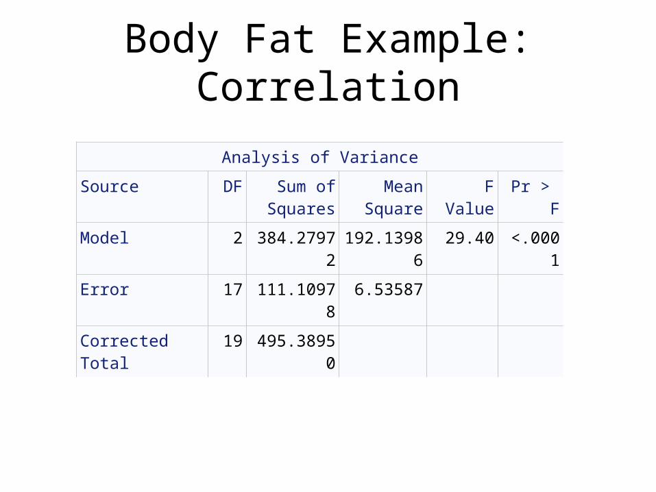
Body Fat Example: Correlation



MeanSquare

F Value Pr > F

Model 2 384.27972 192.13986 29.40 <.0001

Error 17 111.10978 6.53587


Body Fat Example: CorrelationNote: Model is not full rank. Least-squares solutions for the

parameters are not unique. Some statistics will be misleading. A reported DF of 0 or B means that the estimate is biased.

Note: The following parameters have been set to 0, since the variables are a linear combination of other variables as shown.

midarm = thmid - thigh

Parameter Estimates


StandardError

t Value Pr > |t|

Intercept 1 -25.99695 6.99732 -3.72 0.0017

thmid B 0.09603 0.16139 0.60 0.5597

thigh B 0.75485 0.20437 3.69 0.0018

midarm 0 0 . . .

Body Fat Example: Effects of Correlation

Variables in model b1 b2 s{b1} s{b2}

X1 0.8572 0.1288X2 0.8565 0.1100X1, X2 0.2224 0.6594 0.3034 0.2912X1, X2, X3 4.334 -2.857 3.013 2.582

Body Fat Example: Correlation (nknw260.sas)

proc corr data=bodyfat noprob;run;


skinfold thigh midarm fat

skinfold 1.00000 0.92384 0.45778 0.84327

thigh 0.92384 1.00000 0.08467 0.87809

midarm 0.45778 0.08467 1.00000 0.14244

fat 0.84327 0.87809 0.14244 1.00000

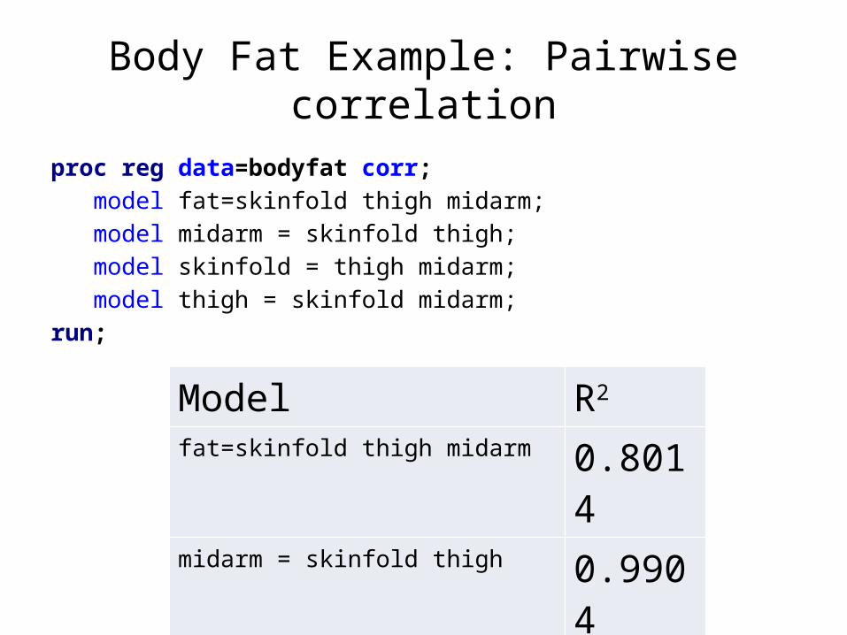
Body Fat Example: Pairwise correlation

proc reg data=bodyfat corr; model fat=skinfold thigh midarm; model midarm = skinfold thigh; model skinfold = thigh midarm; model thigh = skinfold midarm;run;

Model R2

fat=skinfold thigh midarm 0.8014midarm = skinfold thigh 0.9904skinfold = thigh midarm 0.9986thigh = skinfold midarm 0.9982

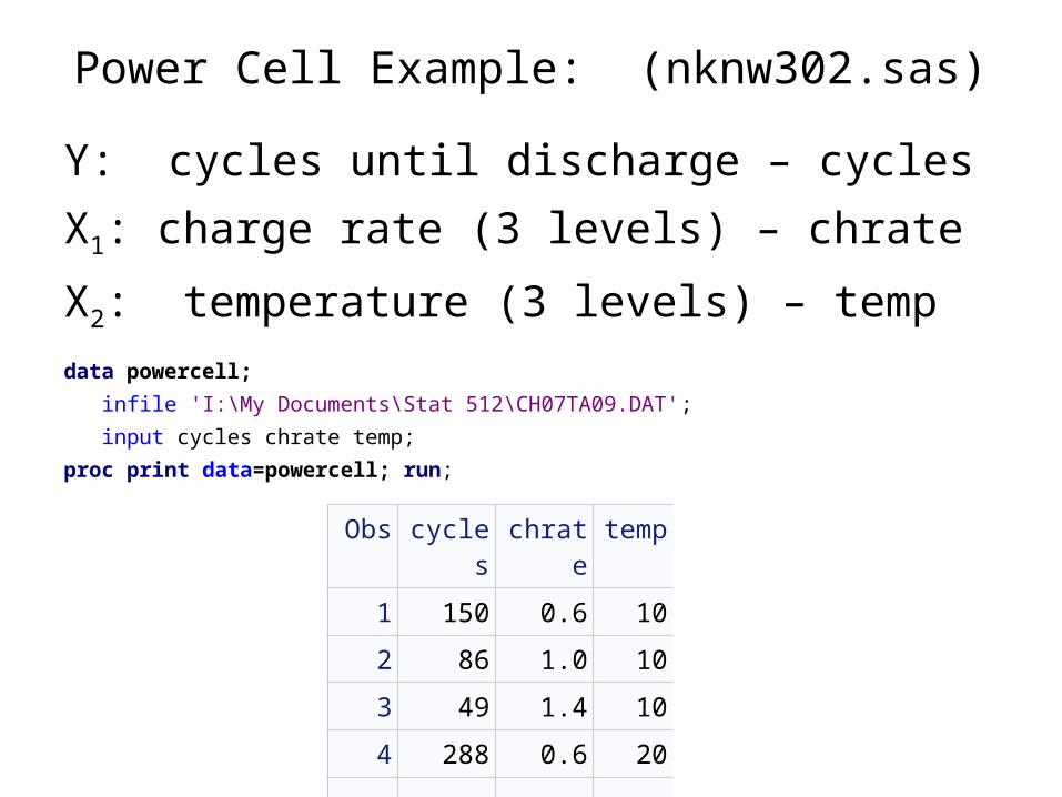
Power Cell Example: (nknw302.sas)

Y: cycles until discharge – cyclesX1: charge rate (3 levels) – chrate

X2: temperature (3 levels) – tempdata powercell; infile 'I:\My Documents\Stat 512\CH07TA09.DAT'; input cycles chrate temp;proc print data=powercell; run;Obs cycles chrate temp

1 150 0.6 10

2 86 1.0 10

3 49 1.4 10

4 288 0.6 20 ⁞ ⁞ ⁞ ⁞

Power Cell Example: Multiple Regression

data powercell; set powercell; chrate2=chrate*chrate; temp2=temp*temp; ct=chrate*temp;

proc reg data=powercell; model cycles=chrate temp chrate2 temp2 ct / ss1 ss2;run;

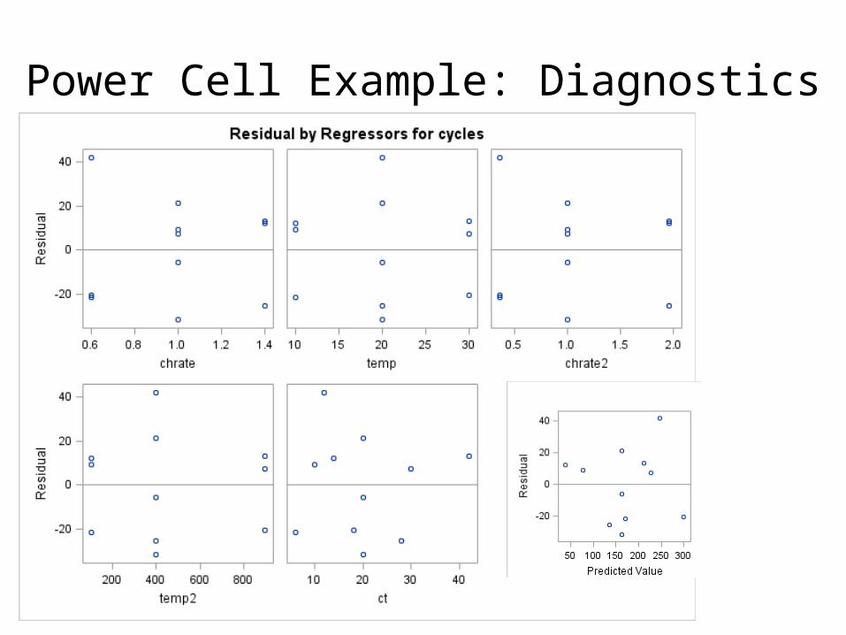
Power Cell Example: Diagnostics

Power Cell Example: Diagnostics

Power Cell Example: Multiple Regression (cont)



MeanSquare

F Value Pr > F

Model 5 55366 11073 10.57 0.0109

Error 5 5240.43860 1048.08772

Corrected Total 10 60606



Coeff Var 18.82220


Parameter Estimates


StandardError

t Value Pr > |t|

Intercept 1 337.72149 149.96163 2.25 0.0741

chrate 1 -539.51754 268.86033 -2.01 0.1011

temp 1 8.91711 9.18249 0.97 0.3761

chrate2 1 171.21711 127.12550 1.35 0.2359

temp2 1 -0.10605 0.20340 -0.52 0.6244

ct 1 2.87500 4.04677 0.71 0.5092


Parameter EstimatesVariable DF Parameter

EstimateStandard

Errort Value Pr > |t| Type I SS Type II SS

Intercept 1 337.72149 149.96163 2.25 0.0741 325424 5315.62944

chrate 1 -539.51754 268.86033 -2.01 0.1011 18704 4220.41673

temp 1 8.91711 9.18249 0.97 0.3761 34202 988.38036

chrate2 1 171.21711 127.12550 1.35 0.2359 1645.96667 1901.19474

temp2 1 -0.10605 0.20340 -0.52 0.6244 284.92807 284.92807

ct 1 2.87500 4.04677 0.71 0.5092 529.00000 529.00000

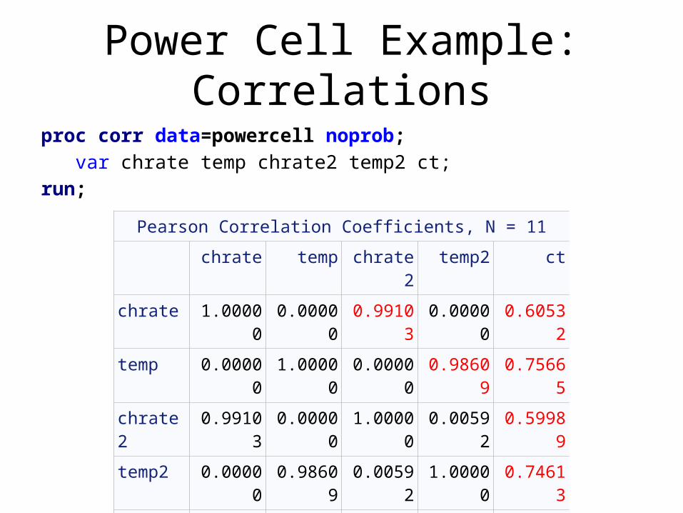
Power Cell Example: Correlationsproc corr data=powercell noprob; var chrate temp chrate2 temp2 ct;run;


chrate temp chrate2 temp2 ct

chrate 1.00000 0.00000 0.99103 0.00000 0.60532

temp 0.00000 1.00000 0.00000 0.98609 0.75665

chrate2 0.99103 0.00000 1.00000 0.00592 0.59989

temp2 0.00000 0.98609 0.00592 1.00000 0.74613

ct 0.60532 0.75665 0.59989 0.74613 1.00000

Power Cell Example: Centeringdata copy; set powercell; schrate=chrate; stemp=temp; drop chrate2 temp2 ct;

proc standard data=copy out=std mean=0; var schrate stemp;* schrate and stemp now have mean 0;proc print data=std;run;

Obs cycles chrate temp schrate stemp

1 150 0.6 10 -0.4 -10

2 86 1.0 10 0.0 -10

3 49 1.4 10 0.4 -10

4 288 0.6 20 -0.4 0

⁞ ⁞ ⁞ ⁞ ⁞ ⁞

Power Cell Example: Centered Variables

data std; set std; schrate2=schrate*schrate; stemp2=stemp*stemp; sct=schrate*stemp;

proc reg data=std; model cycles= chrate temp schrate2 stemp2 sct / ss1 ss2;

Power Cell Example: Centered Variables (cont)


EstimateStandard

Errort Value Pr > |t|

Intercept 1 151.42544 45.45653 3.33 0.0208

chrate 1 -139.58333 33.04176 -4.22 0.0083

temp 1 7.55000 1.32167 5.71 0.0023

schrate2 1 171.21711 127.12550 1.35 0.2359

stemp2 1 -0.10605 0.20340 -0.52 0.6244

sct 1 2.87500 4.04677 0.71 0.5092



EstimateStandard

Errort Value Pr > |t| Type I SS Type II SS

Intercept 1 151.42544 45.45653 3.33 0.0208 325424 11631

chrate 1 -139.58333 33.04176 -4.22 0.0083 18704 18704

temp 1 7.55000 1.32167 5.71 0.0023 34202 34202

schrate2 1 171.21711 127.12550 1.35 0.2359 1645.96667 1901.19474

stemp2 1 -0.10605 0.20340 -0.52 0.6244 284.92807 284.92807

sct 1 2.87500 4.04677 0.71 0.5092 529.00000 529.00000


proc corr data=std noprob;var chrate temp schrate2 stemp2 sct;

run;


chrate temp schrate2 stemp2 sct

chrate 1.00000 0.00000 0.00000 0.00000 0.00000

temp 0.00000 1.00000 0.00000 0.00000 0.00000

schrate2 0.00000 0.00000 1.00000 0.26667 0.00000

stemp2 0.00000 0.00000 0.26667 1.00000 0.00000

sct 0.00000 0.00000 0.00000 0.00000 1.00000

Power Cell Example: Second Orderproc reg data=std; model cycles= chrate temp schrate2 stemp2 sct / ss1 ss2;

second: test schrate2, stemp2, sct;run;

Test second Results for Dependent Variable cycles


F Value Pr > F

Numerator 3 819.96491 0.78 0.5527


Meaning of Coefficients for Qualitative Variables

Insurance Example: Background (nknw459.sas)

Y: number of months for an insurance company to adopt an innovation

X1: size of the firm

X2: Type of firm

X2 = 0 mutual fund firm

X2 = 1 stock firm

Questions1) Do stock firms adopt innovation faster?2) Does the size of the firm have an effect on 1)?

Insurance Example: Inputdata insurance; infile 'I:\My Documents\Stat 512\CH11TA01.DAT'; input months size stock;proc print data=insurance;run;

Obs months size stock1 17 151 02 26 92 0⁞ ⁞ ⁞ ⁞19 30 124 120 14 246 1

Insurance Example: Scatterplotsymbol1 v=M i=sm70 c=black l=1;symbol2 v=S i=sm70 c=red l=3;title1 h=3 'Insurance Innovation';axis1 label=(h=2);axis2 label=(h=2 angle=90);proc sort data=insurance;

by stock size;title2 h=2 'with smoothed lines';proc gplot data=insurance; plot months*size=stock/haxis=axis1 vaxis=axis2;run;

Insurance Example: Scatterplot (cont)

Insurance Example: Regressiondata insurance; set insurance; sizestock=size*stock;run;

proc reg data=insurance; model months = size stock sizestock; sameline: test stock, sizestock;run;

Insurance Example: Regression (cont)

Test sameline Results for Dependent Variable months

Source DFMean

SquareF Value Pr > F

Numerator 2 158.12584 14.34 0.0003Denominator 16 11.02381


Source DFSum of

SquaresMean

SquareF Value Pr > F

Model 3 1504.41904 501.47301 45.49 <.0001Error 16 176.38096 11.02381 Corrected Total 19 1680.80000

Root MSE 3.32021 R-Square 0.8951Dependent Mean 19.40000 Adj R-Sq 0.8754

Insurance Example: Regression (cont)

Parameter Estimates

Variable DFParameter

EstimateStandard


Intercept 1 33.83837 2.44065 13.86 <.0001size 1 -0.10153 0.01305 -7.78 <.0001stock 1 8.13125 3.65405 2.23 0.0408sizestock 1 -0.00041714 0.01833 -0.02 0.9821

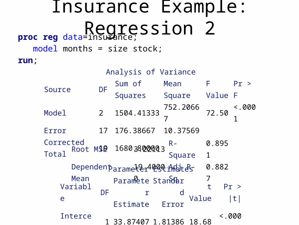
Insurance Example: Regression 2proc reg data=insurance; model months = size stock;run;


Source DFSum ofSquares

MeanSquare

F Value

Pr > F



Parameter Estimates


EstimateStandard


Intercept 1 33.87407 1.81386 18.68 <.0001size 1 -0.10174 0.00889 -11.44 <.0001stock 1 8.05547 1.45911 5.52 <.0001

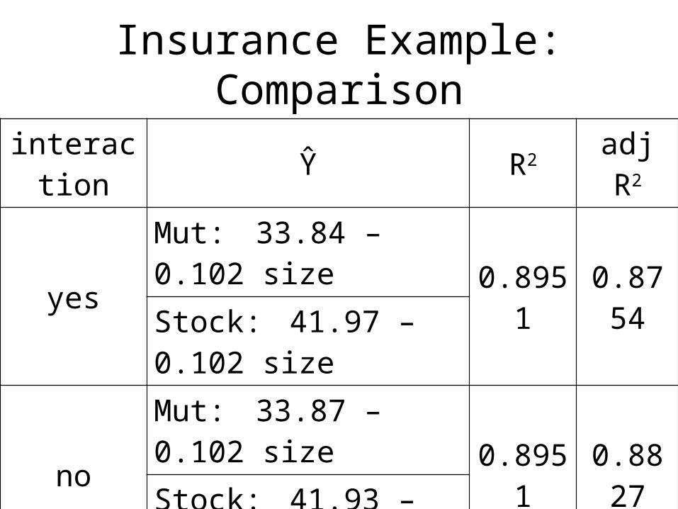
Insurance Example: Comparison

interaction Y R2 adj R2

yesMut: 33.84 – 0.102 size

0.8951 0.8754Stock: 41.97 – 0.102 size

noMut: 33.87 – 0.102 size

0.8951 0.8827Stock: 41.93 – 0.102 size

Insurance Example: Regression 2proc reg data=insurance; model months = size stock;run;


Source DFSum ofSquares

MeanSquare

F Value

Pr > F



Parameter Estimates


EstimateStandard


Intercept 1 33.87407 1.81386 18.68 <.0001size 1 -0.10174 0.00889 -11.44 <.0001stock 1 8.05547 1.45911 5.52 <.0001

Insurance Example: Regression Lines

title2 h=2 'with straight lines';symbol1 v=M i=rl c=black;symbol2 v=S i=rl c=red;proc gplot data=insurance; plot months*size=stock/haxis=axis1 vaxis=axis2;run;

Insurance Example: Regression Lines (cont)

Strategy for Building a Regression Model

Strategy for Building a Regression Model (cont)

Surgical Example (nknw334.sas)

Surgical unit wants to predict survival in patients undergoing a specific liver operation.

n = 54Y = post-operation survival timeExplanatory Variables

X1: blood clotting score (blood)

X2: prognostic index (prog)

X3: enzyme function test score (enz)

X4: liver function test score (liver)

Surgical Example: inputdata surgical; infile 'I:\My Documents\Stat 512\CH09TA01.txt'

delimiter='09'x;input blood prog enz liver age gender alcmod alcheavy surv

logsurv;run;

proc print data=surgical; run;

title1 h=3 'Original model';title2 h=2 'Matrix Scatterplot';proc sgscatter data=surgical; matrix surv blood prog enz liver;run;

Surgical Example: Scatterplot

Surgical Example: Diagnosticsproc reg data=surgical; model surv = blood prog enz liver; output out=diag r=resid p=pred;run;

title1 h=3 'Original model';title2 h=2 'Residual plot vs predicted value';axis1 label=(h=2);axis2 label=(h=2 angle=90);symbol1 v=circle;proc gplot data=diag; plot resid*pred/vref=0 haxis=axis1 vaxis=axis2;run;

title2 'Normal plot for residuals';proc univariate data=diag noprint; histogram resid/normal kernel; qqplot resid/normal (sigma=est mu=est);run;

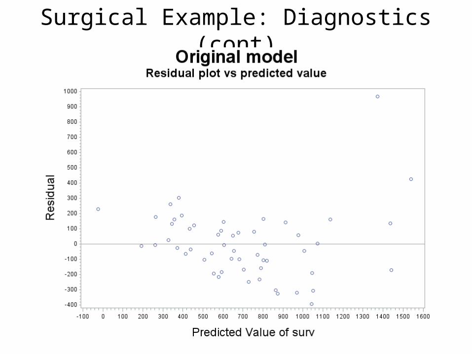
Surgical Example: Diagnostics (cont)



Surgical Example: Y transformationproc transreg data=surgical; model boxcox(surv/lambda=-1 to 1 by 0.1) = identity (blood) identity (prog) identity (enz) identity (liver);run;

Surgical Example: Y transformation (cont)

Surgical Example: Diagnostics 2data surgical; set surgical; lsurv=log(surv);proc reg data=surgical; model lsurv=liver blood prog enz /ss1 ss2; output out=diagtr r=residtr p=predtr;title1 h=3 'Transformed model with ln Y';title2 h=2 'Residual plot vs predicted value';symbol1 v=circle;proc gplot data=diagtr; plot residtr*predtr/vref=0;run;title2 'Normal plot for residuals';proc univariate data=diagtr noprint; histogram residtr/normal kernel; qqplot residtr/normal (sigma=est mu=est);

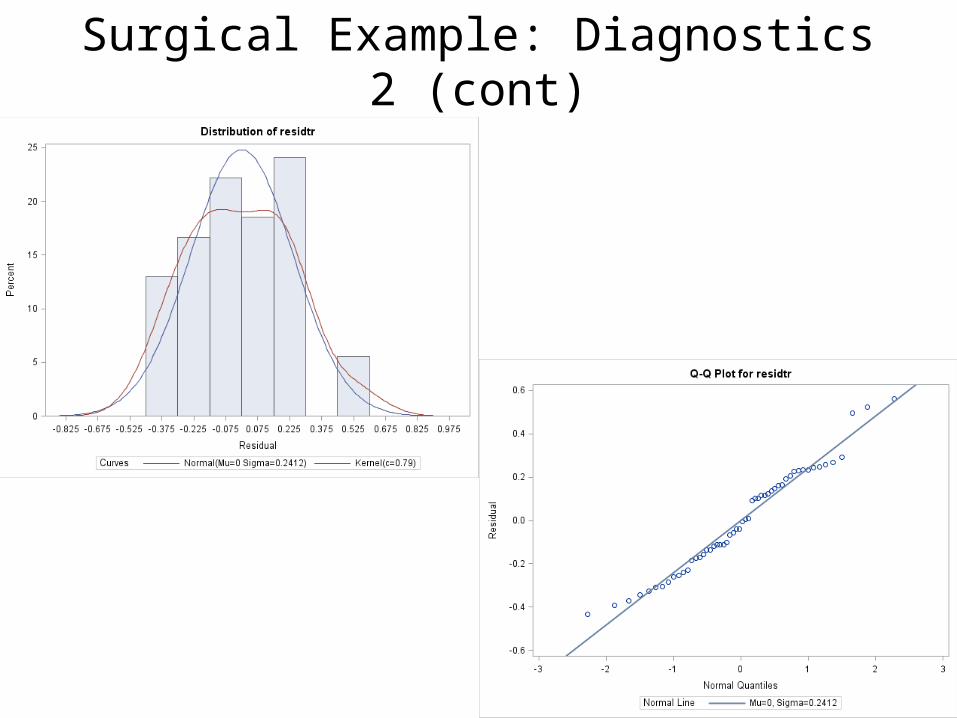
Surgical Example: Diagnostics 2 (cont)



Surgical Example: Scatterplot transformed

title2 h=2 'Matrix Scatterplot';proc sgscatter data=surgical; matrix lsurv blood prog enz liver;run;

Surgical Example: Scatterplot transformed

Surgical Example: Correlationproc corr data=surgical noprob;

var lsurv blood prog enz liver;run;


lsurv blood prog enz liver

lsurv 1.00000 0.24633 0.47015 0.65365 0.64920

blood 0.24633 1.00000 0.09012 -0.14963 0.50242

prog 0.47015 0.09012 1.00000 -0.02361 0.36903

enz 0.65365 -0.14963 -0.02361 1.00000 0.41642

liver 0.64920 0.50242 0.36903 0.41642 1.00000

Surgical Example: Model Selection – data for the current model

proc reg data=surgical outtest=mparam; model lsurv=blood prog enz liver/ rsquare adjrsq cp press aic sbc;run;proc print data=mparam; run;

Obs _MODEL_ _TYPE_ _DEPVAR_ _RMSE_ _PRESS_

1 MODEL1 PARMS lsurv 0.25088 4.06875

Obs _IN_ _P_ _EDF_ _RSQ_ _ADJRSQ_ _CP_ _AIC_ _SBC_

1 4 5 49 0.75914 0.73948 5 -144.587 -134.642

Obs Intercept blood prog enz liver lsurv

1 3.85193 0.083739 0.012671 0.015627 0.032056 -1

Surgical Example: Model Selection – all subset selection

proc reg data=surgical; model lsurv=blood prog enz liver/ selection=rsquare adjrsq cp b best=3;run;

Surgical Example: Model Selection – all subset selection (cont)

Number in Model

R-Square Adjusted R-Square

C(p) Parameter Estimates

Intercept blood prog enz liver

1 0.4273 0.4162 66.5181 5.26489 . . 0.01512 .

1 0.4215 0.4103 67.6959 5.61241 . . . 0.29812

1 0.2210 0.2061 108.4692 5.56592 . 0.01367 . .

2 0.6632 0.6500 20.5228 4.35094 . 0.01413 0.01538 .

2 0.5992 0.5835 33.5362 5.02882 . . 0.01072 0.20945

2 0.5484 0.5307 43.8729 4.54673 0.10794 . 0.01633 .

3 0.7572 0.7427 3.3879 3.76644 0.09547 0.01334 0.01644 .

3 0.7177 0.7007 11.4343 4.40617 . 0.01101 0.01260 0.12973

3 0.6119 0.5886 32.9601 4.78212 0.04485 . 0.01219 0.16356

4 0.7591 0.7395 5.0000 3.85193 0.08374 0.01267 0.01563 0.03206

Surgical Example: Model Selection – all subset selection (cont)

Number inModel

R-Square AdjustedR-Square

C(p) Variables in Model

1 0.4273 0.4162 66.5181 enz1 0.4215 0.4103 67.6959 liver1 0.2210 0.2061 108.4692 prog2 0.6632 0.6500 20.5228 prog enz2 0.5992 0.5835 33.5362 enz liver2 0.5484 0.5307 43.8729 blood enz3 0.7572 0.7427 3.3879 blood prog enz3 0.7177 0.7007 11.4343 prog enz liver3 0.6119 0.5886 32.9601 blood enz liver4 0.7591 0.7395 5.0000 blood prog enz liver

proc reg data=surgical; model lsurv=blood prog enz liver/ selection=rsquare adjrsq cp best=3;run;

Surgical Example: Type II SSproc reg data=surgical; model lsurv=blood prog enz liver/ss1 ss2; output out=diagtr r=residtr p=predtr;run; Parameter Estimates

Variable DF Parameter Estimate

Standard Error

t Value Pr > |t| Type I SS Type II SS

Intercept 1 3.85193 0.26626 14.47 <.0001 2233.00123 13.17242

blood 1 0.08374 0.02883 2.90 0.0055 0.77696 0.53086

prog 1 0.01267 0.00231 5.47 <.0001 2.59042 1.88571

enz 1 0.01563 0.00210 7.44 <.0001 6.32862 3.48424

liver 1 0.03206 0.05147 0.62 0.5363 0.02442 0.02442

Surgical Example: Model Selection - automatic

proc reg data=surgical; model lsurv=blood prog enz liver / selection=stepwise;run;

All variables left in the model are significant at the 0.1500 level. No other variable met the 0.1500 significance level for entry into the model.

Summary of Stepwise Selection

Step Variable Entered

Variable Removed

Number Vars In

Partial R-Square

Model R-Square

C(p) F Value Pr > F

1 enz 1 0.4273 0.4273 66.5181 38.79 <.0001

2 prog 2 0.2359 0.6632 20.5228 35.72 <.0001

3 blood 3 0.0941 0.7572 3.3879 19.37 <.0001

Surgical Example: Model Selection – backward elimination

Bounds on condition number: 1.0308, 9.1864 All variables left in the model are significant at the 0.1000 level.

Variable Parameter Estimate

Standard Error

Type II SS F Value Pr > F

Intercept 3.76644 0.22676 17.15229 275.89 <.0001

blood 0.09547 0.02169 1.20436 19.37 <.0001

prog 0.01334 0.00203 2.67403 43.01 <.0001

enz 0.01644 0.00163 6.32862 101.80 <.0001

Summary of Backward Elimination

Step Variable Removed

Number Vars In

Partial R-Square

Model R-Square

C(p) F Value Pr > F

1 liver 3 0.0019 0.7572 3.3879 0.39 0.5363

CS Example: General Linear Test (cs2.sas) proc reg data=cs; model gpa=satm satv hsm hss hse; * test H0: beta1 = beta2 = 0; sat: test satm, satv; * test.

Documents

body fat example

test skinfold

thigh model fat

square f valuepr f model3396

general linear test

skinfold model fat

bodyfat model fat

test thigh results