Crossover Design - Biostatistics - Academic Divisions

PubH 7405: REGRESSION ANALYSIS

CROSS-OVER EXPERIMENT DESIGNS

THE ROLE OF STUDY DESIGN In a “standard” experimental design, a linear model for a continuous response/outcome is:

+

+

=

ErroralExperiment

EffectTreatment

ConstantOverall

Y

The last component, ‘experimental error”, includes not only error specific to the experimental process but also includes “subject effect” (age, gender, etc…). Sometimes these subject effects are large making it difficult to assess “treatment effect”.

Blocking (to turn a completely randomized design into a randomized complete block design ) would help. But it would only help to “reduce” subject effects, not to “eliminate” them: subjects in the same block are only similar, not identical – unless we have “blocks of size one”. And that the basic idea of “Cross-over Design”, a very popular form in biomedical research.

Cross-over is a very special design where we have “bloc” of size one; each subject serves as his/her own control receiving both treatment. Randomization decides the order. The outcome could be binary or on the continuous scale.

Let start with the case of a continuous outcome and, for illustration, consider a project we just completed here: a clinical trial to prevent lung cancers.

US Mortality, 2006

Source: US Mortality Data 2006, National Center for Health Statistics, Centers for Disease Control and Prevention, 2009.

1. Heart Diseases 631,636 26.0 2. Cancer 559,888 23.1 3. Cerebrovascular diseases 137,119 5.7 4. Chronic lower respiratory diseases 124,583 5.1 5. Accidents (unintentional injuries) 121,599 5.0 6. Diabetes mellitus 72,449 3.0 7. Alzheimer disease 72,432 3.0 8. Influenza & pneumonia 56,326 2.3 9. Nephritis 45,344 1.9 10. Septicemia 34,234 1.4

Rank Cause of Death No. of deaths

% of all deaths

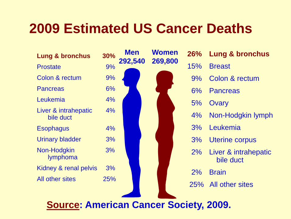
2009 Estimated US Cancer Deaths

Source: American Cancer Society, 2009.

Men 292,540

Women 269,800

26% Lung & bronchus 15% Breast

9% Colon & rectum

6% Pancreas

5% Ovary

4% Non-Hodgkin lymph

3% Leukemia

3% Uterine corpus

2% Liver & intrahepatic bile duct

2% Brain

25% All other sites

Lung & bronchus 30% Prostate 9%

Colon & rectum 9%

Pancreas 6%

Leukemia 4%

Liver & intrahepatic 4% bile duct

Esophagus 4%

Urinary bladder 3%

Non-Hodgkin 3% lymphoma

Kidney & renal pelvis 3%

All other sites 25%

Cancer Death Rates Among Men, US,1930-2005

Source: US Mortality Data 1960-2005, US Mortality Volumes 1930-1959, National Center for Health Statistics, Centers for Disease Control and Prevention, 2008.

0

20

40

60

80

10019

30

1935

1940

1945

1950

1955

1960

1965

1970

1975

1980

1985

1990

1995

2000

2005

Lung & bronchus

Colon & rectum

Stomach

Rate Per 100,000

Prostate

Pancreas

Liver Leukemia

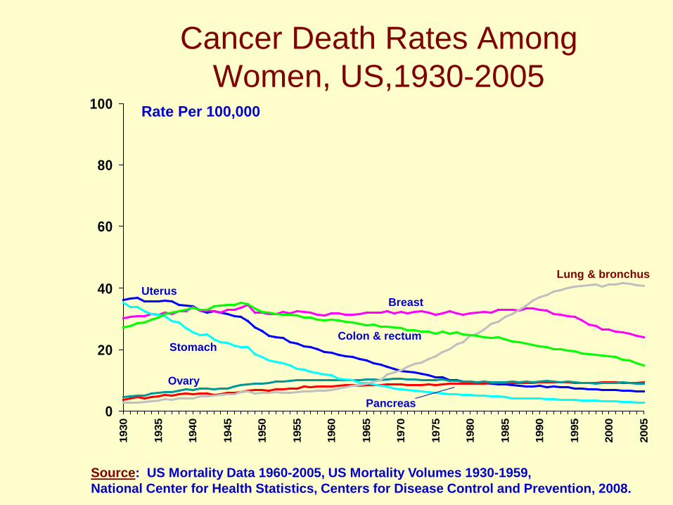
Cancer Death Rates Among Women, US,1930-2005

Source: US Mortality Data 1960-2005, US Mortality Volumes 1930-1959, National Center for Health Statistics, Centers for Disease Control and Prevention, 2008.

0

20

40

60

80

10019

30

1935

1940

1945

1950

1955

1960

1965

1970

1975

1980

1985

1990

1995

2000

2005

Lung & bronchus

Colon & rectum

Uterus

Stomach

Breast

Ovary

Pancreas

Rate Per 100,000

Lung cancer is the leading cause of cancer death in the United States and worldwide. Cigarette smoking causes approximately 90% of lung cancer. Despite anti-smoking campaigns over the past 40 years, over 45 million (22%) adult Americans are still current smokers. The development of a viable chemoprevention strategy targeting current smokers potentially could decrease lung cancer mortality.

Previous studies have shown

(1) that the tobacco specific nitrosamine 4(methylnitrosamino)-1-(3-pyridyl)-1-butanone (NNK) is a major lung carcinogen in tobacco smoke,

(2) that 2-phenethyl isothiocyanate (PEITC) is a potent inhibitor of NNK-induced lung carcinogenesis in rats and mice.

PEITC can be found in water cress, garden cress, broccoli, among other foods; but few people eat enough of those foods. We extract PEITC from foods then form pills having higher concentration.

Then we designed and conducted a placebo-controlled cross-over clinical trial to assess the effect of a PEITC supplement on changes of NNK metabolism in smokers. We hypothesize that there will be a 30% increase in urinary NNAL plus NNAL-Gluc among PEITC treated subjects (taking more toxin out).

In the most simple cross-over design, subjects are randomly divided into two groups (often of equal sign); subjects in both groups/series take both treatments (experimental treatment and placebo/control) but in different “orders”.

Of course, “order effects” and “carry-over effects” are possible. And the cross-over designs are not always suitable. They are commonly used when treatment effects are not permanent; for example some treatments of rheumatism.

THE DESIGN In our “PEITC trial”, measurements (urinary total NNAL) will be taken from each subject in the two supplementation sequences as seen in the following diagram: Group 1: Period #1 (PEITC; A1) – washout – Period #2 (Placebo; B2) Group 2: Period #1 (Placebo; B1) – washout – Period #2 (PEITC; A2) The letter is used to denote supplementation or treatment (A for PEITC and B for Placebo) and the number, 1 or 2, denotes the period; e.g. “A1” for PEITC taken in period #1.

The “washout periods” are inserted in order to eliminate possible “carry-over effects” (The half-life of dietary PEITC in vivo is between 2-3 hours, with complete excretion within 1-2 days following ingestion).

There are more complicated designs in which three treatments, in different orders, are compared a three-sequence, three-period trial – with two washout periods.

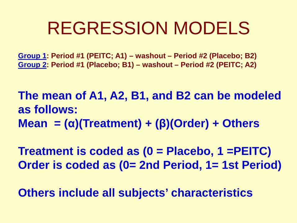
REGRESSION MODELS

The mean of A1, A2, B1, and B2 can be modeled as follows: Mean = (α)(Treatment) + (β)(Order) + Others Treatment is coded as (0 = Placebo, 1 =PEITC) Order is coded as (0= 2nd Period, 1= 1st Period) Others include all subjects’ characteristics

Group 1: Period #1 (PEITC; A1) – washout – Period #2 (Placebo; B2) Group 2: Period #1 (Placebo; B1) – washout – Period #2 (PEITC; A2)

OUTCOME VARIABLE From the design: Group 1: Period #1 (PEITC; A1) – washout – Period #2 (Placebo; B2) Group 2: Period #1 (Placebo; B1) – washout – Period #2 (PEITC; A2) Our data analysis could be based on the following “outcome variables” (Treatment - Placebo): X1 = A1 - B2; and X2 = A2 - B1 This subtraction will cancel the “within-sequence” effects of all subject-specific factors. This process will result in two independent samples (often with the same or similar sample size if there are no or minimal dropouts or missing data).

Recall the general model: The subtractions X1 = A1 - B2; and X2 = A2 - B1 will cancel not only effects of all subject-specific factors; they cancel the “overall constant” as well, leaving only two parameters in the means of X1 and X2: Mean of X1 = [(α)(1)+(β)(1)] – [(α)(0)+(β)(0)] = α + β Mean of X2 = [(α)(1)+(β)(0)] – [(α)(0)+(β)(1)] = α - β

+

+

=

ErroralExperiment

EffectTreatment

ConstantOverall

Y

RESULTING LINEAR MODELS Design: Group 1: Period #1 (PEITC; A1) – washout – Period #2 (Placebo; B2) Group 2: Period #1 (Placebo; B1) – washout – Period #2 (PEITC; A2) Outcome variables: X1 = A1 - B2; and X2 = A2 - B1 Resulting Linear regression models: X1 is normally distributed as N(α+β,σ2) X2 is normally distributed as N(α-β,σ2) In this models, α represents the PEITC supplementation effect (α>0 if and only if PEITC increases the total NNAL) and β represents the period effect (β>0 if and only if measurement from period 1 is larger than from period 2).

(1) The X’s do not really need to have normal distributions; the robustness comes from the fact that our analysis will be based on the normal distribution of the sample mean – not of the data, and the sample mean would be almost normally distribution for moderate to large sample sizes (Central Limit Theorem).

(2) Among the three parameters, α represents the

PEITC effect and is the primary target, β could be of some interest; we have no in σ2 (we have to handle it properly to make inferences on α (and β) valid and efficient.

DATA ANALYSIS Design: Group 1: Period #1 (PEITC; A1) – washout – Period #2 (Placebo; B2) Group 2: Period #1 (Placebo; B1) – washout – Period #2 (PEITC; A2) Outcome variables: X1 = A1 - B2; and X2 = A2 - B1 From the model: X1 is normally distributed as N(α+β,σ2) X2 is normally distributed as N(α-β,σ2) Let the sample means and sample variances be defined as usual and n the group size (total sample size is 2n); then, we can easily prove the followings:

TREATMENT EFFECTS

)2nσN(α normal as is a

2xxa

2

_

2

_

1

,

),(N normal as is

),,(N normal as is

2_

2

2_

1

ddistribute

nddistributex

nddistributex

+=

−

+

σβα

σβα

ESTIMATION OF PARAMETERS (1) Estimation of Variance. We can pool data from the two

sequences to estimate the common variance σ2 by sp2

– the same pooled estimate used in two-sample t-test. (2) Estimation of Treatment Effect. Parameter α

representing the PEITC effect, the difference between PEITC and the placebo, is estimated by a – the average of the two sample means. Its 95 percent confidence interval is given by:

Ns

ta p975.±

The t-coefficient goes with (N-2) degrees of freedom; without missing data, N = 2n – total number of subjects.

TESTING FOR TREATMENT EFFECT Testing for PEITC Treatment Effect: Null hypothesis

of “no treatment effects” H0: α = 0 is tested using the “t test”, with (N-2) degrees of freedom:

N/sat

p

=

It’s kind of “one-sample t-test” but we use the degree of freedom associated with sp. Alternatively, one can frame it as a two-sample t-test comparing the mean of X1 versus the mean of (-X2) as seen from X1 is normally distributed as N(α+β,σ2) X2 is normally distributed as N(α-β,σ2)

ORDER EFFECTS

)2nσN(β normal as is b

2xxb

2

_

2

_

1

,

),(N normal as is

),,(N normal as is

2_

2

2_

1

ddistribute

nddistributex

nddistributex

−=

−

+

σβα

σβα

ESTIMATION OF PARAMETERS (1) Estimation of Variance. We can pool data from the two

sequences to estimate the common variance σ2 by sp2

– the same pooled estimate used in two-sample t-test. (2) Estimation of Order Effect: Parameter β representing

the order effect, the difference between Period 1 and Period 2, is estimated by b – half the difference of the two sample means. Its 95 percent confidence interval is given by:

Ns

tb p975.±

The t-coefficient goes with (N-2) degrees of freedom; without missing data, N = 2n – total number of subjects.

TESTING FOR ORDER EFFECT Testing for Order Effect: Null hypothesis of “no order

effects” H0: β = 0 is tested using the “t test”, with (N-2) degrees of freedom:

N/sbt

p

=

It’s kind of “one-sample t-test” but we use the degree of freedom associated with sp. Alternatively, one can frame it as a two-sample t-test comparing the mean of X1 versus the mean of X2 as seen from X1 is normally distributed as N(α+β,σ2) X2 is normally distributed as N(α-β,σ2)

Two-period crossover designs are often used in clinical trials in order to improved sensitivity of the trial by eliminating individual patient effects. They have been popular in dairy husbandry studies, long-term agricultural experiments, bioavailability and bioequivalence studies, nutrition experiments, arthritic and periodontal studies, and educational and psychological studies – where treatment effects are not permanent.

The response could be quantitative but quite often the response variable is binary , e.g. the response is whether or not relief from pain is obtained.

THE DESIGN

Recall the following design; the only difference is that, in this case, the four outcomes A1, A2, B1, and B2 are binary – say 1 if positive response and 0 otherwise: Group 1: Period #1 (Trt A; A1) – washout – Period #2 (Trt B; B2) Group 2: Period #1 (Trt B; B1) – washout – Period #2 (Trt A; A2) The washout periods are optional and the group sizes could be different (due to dropouts) – but not by much.

In general, let Y be the outcome or dependent variable taking on values 0 and 1, and: π = Pr(Y=1) Y is said to have the “Bernouilli distribution” (Binomial with n = 1). We have:

)1()()(

πππ

−==

YVarYE

Studies would involve some independent variables (treatment, order, etc…)

Let π be the probability (also the mean of the Bernouilli distribution) and X a covariate (let consider only one X for simplicity). The common step in the regression modeling process is to relate π and X using the Logistic Regression Model – as follows.

LOGISTIC REGRESSION

xββπ1

πlog

e1eπ

10

xββ

xββ

10

10

+=−

=−

+=−

+=

+

+

+

+

x

x

e

e10

10

1

111

ββ

ββ

ππ

π

“Logistic Simple Linear Regression”

THE LOGISTIC MODELS

The Multiple Logistic Models for cross-over design are ( J. J. Gart, Biometrika 1969):

βαλ

βαλ

βαλ

βαλ

βαλ

βαλ

βαλ

βαλ

i

i

i

i

i

i

i

i

e1e1)Pr(A2;

e1e1)Pr(B1

e1e1)Pr(B2;

e1e1)Pr(A1

−+

−+

+−

+−

++

−−

++

++

+==

+==

+==

+==

In this models, (1) λ‘s represent the subjects effects varying from subject to subject; could be many terms here. (2) α represents the new treatment effect, say PEITC supplementation, (α>0 if and only if PEITC is more effective) – our main interest - and (3) β represents the period effect (β>0 if and only if a treatment from period 1 is more effective than from period 2).

In this modeling:

(1) We “code” binary covariates (Treatment and Order) as (+1/-1) instead of (0,1);

(2) All subject-specific covariates are lumped together with the Intercept.

We want to eliminate the subjects’ effects in drawing inferences on treatment and order effects. However, we cannot simply do some subtractions like (X1 = A1 - B2 and X2 = A2 - B1). For a continuous outcome, the difference of two normal variables is distributed as “normal”. But this is not true for the Bernouilli distribution.

A viable alternative is a “Conditional Analysis”, like the formation of the McNemar Chi-square test – used, for example, in the analysis of pair-matched case-control studies.

It was shown by Gart (1969) that optimum inferences about treatment and order effects, regarding subjects effects as nuisance, are based on those subjects with unlike responses in two periods; that are subjects whose pair of outcomes are either (0,1) or (1,0). This is similar to the argument leading to the McNemar Chi-square test.

# 1: Period 1 (Trt A; A1) – Period 2 (Trt B; B2) # 2: Period 1 (Trt B; B1) – Period 2 (Trt A; A2)

The analysis will be conditioned on:

A1+B2 = 1, and

B1+A2 = 1

βαλ

βαλ

βαλ

βαλ

βαλ

βαλ

βαλ

βαλ

i

i

i

i

i

i

i

i

e1e1)Pr(A2;

e1e1)Pr(B1

e1e1)Pr(B2;

e1e1)Pr(A1

−+

−+

+−

+−

++

−−

++

++

+==

+==

+==

+==

1)0)Pr(B2Pr(A10)1)Pr(B2Pr(A10)1)Pr(B2Pr(A1

1)B20,Pr(A10)B21,Pr(A10)B21,Pr(A11)B2A1|1Pr(A1

==+====

=

==+====

==+=

Recall The Bayes Theorem:

β)2(α

β)2(α

e111)A2B1|1Pr(A2

e11

1)0)Pr(B2Pr(A10)1)Pr(B2Pr(A10)1)Pr(B2Pr(A1

1)B20,Pr(A10)B21,Pr(A10)B21,Pr(A11)B2A1|1Pr(A1

−−

+−

+==+=

+=

==+====

=

==+====

==+=

β)α2(

β)2(α

β)2(α

β)2(α

e111)A2B1|1Pr(B1

e1111)A2B1|1Pr(B1

e111)A2B1|1Pr(A2

e111)B2A1|1Pr(A1

+−−

−−

−−

+−

+==+=

+−==+=

+==+=

+==+=

Data #1: Frequencies of subjects with different Outcomes (0,1) and (1,0)

Treatments (A,B) Treatments (B,A)Oucome A=1 ya1 ya2

Oucome B=1 yb2 yb1

Total n1 n2

p2e111)A2B1|1Pr(A2

p1e111)B2A1|1Pr(A1

β)2(α

β)2(α

=+

==+=

=+

==+=

−−

+−


Oucome B=1 yb2 yb1

Total n1 n2

Results: With n1 and n2 fixed, ya1 and ya2 are distributed as Binomials B(n1,p1) and B(n2,p2)

Note: If there are no Order Effects, then p1 = p2

Data #1: Frequencies of subjects with different Outcomes (0,1) and (1,0)


Oucome B=1 yb2 yb1

Total n1 n2

Testing for Order Effects H0: β = 0 Chi-square test; even Fisher’s Exact Test

Data #2: The same set of data can also be assembled into a different 2x2 Table

Treatments (A,B) Treatments (B,A)1st Outcome=1 ya1 yb1

2nd Outcome =1 yb2 ya2

Total n1 n2

q2e1

11)A2B1|1Pr(B1

p1e111)B2A1|1Pr(A1

β)α2(

β)2(α

=+

==+=

=+

==+=

+−−

+−

Treatments (A,B) Treatments (B,A)1st Oucome=1 ya1 yb1

2nd Oucome=1 yb2 ya2

Total n1 n2

Results: With n1 and n2 fixed, ya1 and yb1 are distributed as Binomials B(n1,p1) and B(n2,q2)

Note: If no Treatment Effects, then p1 = q2

Data #2: The same set of data can also be assembled into a different 2x2 Table

Treatments (A,B) Treatments (B,A)1st Outcome=1 ya1 yb1

2nd Outcome =1 yb2 ya2

Total n1 n2

Testing for Treatment Effects H0: α = 0 Chi-square test; even Fisher’s Exact Test

ESTIMATION OF PARAMETERS

p2e111)A2B1|1Pr(A2

p1e111)B2A1|1Pr(A1

β)2(α

β)2(α

=+

==+=

=+

==+=

−−

+−


Oucome B=1 yb1 yb2

Total n1 n2



(Conditional) Likelihood Function:

b2a2b1a1 yy

a2

2yy

a1

1 p2)(1p2yn

p1)(1p1yn

L −

−

=

β)2(α

β)2(α

e11

e11

−−

+−

+=

+=

2

1

p

p

{ }[ ]

[ ] [ ] 21

a2a1

nα)2(βnβ)2(α

b2b1a2

2

a1

1

y2y

a2

2y1y

a1

1

e1e1

α)(β2yβ)(α2yexpyn

yn

p2)(1p2yn

p1)(1p1yn

L

−+− ++

−++−

=

−

−

=

RESULTS: Estimates & Standard Errors

+==

==

==

b2a2

ba

b1a1

ab

b1a2

b2a1^

b2b1

a2a1^

yyn

yyn

161Var(b)Var(a)

yyyyln

41bβ

yyyyln

41aα

21.1 We conducted a randomized, crossover trial to test whether 3,3'-diindolylmethane (DIM, a metabolite of I3C) excreted in the urine after consumption of raw Brassica vegetables with divergent glucobrassicin concentrations is a marker of I3C uptake from such foods. Twenty-five subjects were fed 50 g of either raw "Jade Cross" Brussels sprouts (high glucobrassicin concentration) or "Blue Dynasty" cabbage (low glucobrassicin concentration) once daily for 3 days. All urine was collected for 24 hours after vegetable consumption each day. After a washout period, subjects crossed over to the alternate vegetable. Data are in file “Brussels Sprouts”; use average of 3 days as our outcome. Estimate & Test for Treatment effects using both the t-test (hand calculation) and SAS program (handout).

DUE AS HOMEWORK

Crossover Design - Biostatistics - Academic Divisions

Documents