Crossover Between the Electron-Hole Phase and the BCS Excitonic Phase in Quantum Dots

January 10, 2000 18:29 WSPC/140-IJMPB 0255

International Journal of Modern Physics B, Vol. 14, No. 1 (2000) 71–83c© World Scientific Publishing Company

CROSSOVER BETWEEN THE ELECTRON HOLE PHASE

AND THE BCS EXCITONIC PHASE IN QUANTUM DOTS

BORIS A. RODRIGUEZ∗

Departamento de Fisica, Universidad de Antioquia,AA 1226, Medellin, Colombia

AUGUSTO GONZALEZ†

Instituto de Cibernetica, Matematica y Fisica Calle E 309,Vedado, Habana 4, Cuba

LUIS QUIROGA‡ and FERNEY J. RODRIGUEZ§

Departamento de Fisica, Universidad de los Andes,AA 4976, Bogota, Colombia

ROBERTO CAPOTE¶

Centro de Estudios Aplicados al Desarrollo Nuclear,Calle 30 No 502, Miramar, La Habana, Cuba

Received 26 October 1999

Second order perturbation theory and a Lipkin–Nogami scheme combined with an exactMonte Carlo projection after variation are applied to compute the ground-state energy of6 ≤ N ≤ 210 electron–hole pairs confined in a parabolic two-dimensional quantum dot.The energy shows nice scaling properties as N or the confinement strength is varied. A

crossover from the high-density electron–hole phase to the BCS excitonic phase is foundat a density which is roughly four times the close-packing density of excitons.

1. Introduction

As we understand, the interest in electron–hole states (excitons) in semiconduc-

tor physics is motivated by two facts. First, excitons have a bosonic character (as

they are made up of a pair of fermions) and, thus, the many-exciton system is a

candidate for a Bose condensate. This possibility was envisaged long ago,1 but re-

gained attention in the last years after the Bose condensation of alcali atoms was

∗E-mail: [email protected]†E-mail: [email protected]‡E-mail: [email protected]§E-mail: [email protected]¶E-mail: [email protected]

71


72 B. A. Rodriguez et al.

achieved.2 Experimentally, signals of Bose–Einstein statistics have been identified in

the photoluminiscence of quantum wells under strong laser pumping,3 and indirect

excitons in quantum wells are being manipulated via applied stress and inhomoge-

neous electric fields4 to reach the densities needed for Bose condensation. On the

other hand, excitons are at the basis of many optical properties of semiconductors.5

Recent experimental works have focused on the lowest dimensional structures, and

very interesting properties have been found in the photoluminiscence of quantum

wires6 and single quantum dots.7

In the present paper, we study a two-dimensional quantum dot with a number

of electron–hole pairs, 6 ≤ N ≤ 210, i.e. intermediate between the very small dot7

and the quantum well.3 We study the dot at strong and intermediate confinement

regimes by means of second-order perturbation theory and a variational (BCS)

procedure. The main results of the paper may be summarised as follows. We found

a breakdown of perturbation theory and a significant BCS pairing roughly at the

same confinement strength, corresponding approximately to four times the close-

packing density of excitons (or four times the Mott transition density). We notice

that the BCS calculations were performed within the Lipkin–Nogami scheme8 with

exact projection onto the N -pair sector9 to avoid the incorrect behaviour of the

naive BCS function in a finite system.10 Second, we found that the energy depends

on N and the confinement strength in a scaled way.

Our paper is complementary to Refs. 11 and 12, in which the multiexcitonic

quantum dot is also studied. In Ref. 11, we found that the far-infrared absorp-

tion of the dot is dominated by a giant-dipole resonance similar to the collective

state appearing in nuclei13 and metallic clusters.14 In paper,12 the Bethe–Goldstone

equations (the independent-pair approximation in Nuclear Physics15) are applied

to study small (2 ≤ N ≤ 6) clusters. The frequency for optical absorption with

creation of an electron–hole pair shows a very interesting behaviour related to the

apparent instability of the free (not confined) four-exciton cluster in two dimensions.

The organisation of the paper is as follows. In Sec. 2, we present the results of

perturbation theory. In Sec. 3, variational (BCS-like) bounds are derived. Projection

onto the N -pair sector is carried out by means of the Lipkin–Nogami combined with

an exact Monte Carlo projection. In Sec. 4, we summarise our main results.

2. Perturbation Theory

We study a direct-band-gap semiconductor with two parabolic bands. N electrons

andN holes are created by, e.g. strong laser pumping. We shall ignore recombination

processes and electron–hole exchange. A model like this have been employed for the

analysis of collective excitations in bulk semiconductors.16 The particles are forced

to move in a two-dimensional region confined by a parabolic potential. This is a

common approach in the study of self-assembled quantum dots.17 For simplicity,

we take mh = me and the same confining potential for both particles. Up to 210

electron–hole pairs will be allowed in the dot.


Crossover Between The Dense Electron–Hole Phase and the BCS Excitonic Phase 73

The Hamiltonian of the system in oscillator units is written as

H

~ω=

1

2

2N∑α=1

(p2α + r2

α) + β∑α<γ

qαqγ

|rα − rγ |, (1)

where ω is the dot frequency, qα = −1 for electrons and +1 for holes. This Hamil-

tonian depends only on one constant, β =√

(me4/κ2~2)/~ω =√Ec/~ω, where

Ec is the Coulomb characteristic energy. m is the electron effective mass, and κ

the dielectric constant of the material. In these units, the effective Bohr radius is

aB = 1/β.

β → 0 is a high-density (strong confinement) limit in which the Bohr radius is

much higher than the oscillator length (equal to one in our units). The independent-

electron and hole picture works in this limit, and the Coulomb interaction may be

computed in perturbation theory. Notice that at high density, we have a system

of independent fermions, not bosons. This is one of the reasons preventing Bose

condensation of excitons in homogeneous 3D systems.1

On the other hand, as β is increased, the dynamics become more and more

dictated by the Coulomb forces. First, we shall observe the emergence of two-body

correlations and the formation of electron–hole “Cooper” pairs (i.e. pairing in Fock

space). With a further increase in β, small excitons, biexcitons and higher complexes

shall start playing a dominant role.

Let us first consider the β → 0 limit, in which the Coulomb interaction may

be computed in perturbation theory. We will make an additional simplifying as-

sumption: N is such that there are Nshell closed shells in the β = 0 limit, that is

the number of electrons takes one of the following values N = Nshell(Nshell + 1) =

6, 12, 20, 30, 42, . . . , 210. The ground state of such systems for small β values is spin-

unpolarised, which means that both the electron and hole subsystems have total

spin S = 0. The angular momentum of this state is L = 0.

The β → 0 perturbative series take the form

E

~ω= b0 + b1β + b2β

2 +O(β3) , (2)

where, the leading approximation to the energy is twice the energy ofN independent

electrons (or holes)

b0 =2

3N√

4N + 1 , (3)

and for b1 and b2 we arrive to the following expressions

b1 = −2∑

n1≤N/2

⟨n1, n1

∣∣∣∣1r∣∣∣∣n1, n1

⟩− 4

∑n1<n2≤N/2

⟨n1, n2

∣∣∣∣1r∣∣∣∣n2, n1

⟩, (4)



b2 = −4∑

n1≤N/2

∑n2>N/2

∣∣∣∑n≤N/2〈n2, n|1/r|n, n1〉∣∣∣2

ε(n2)− ε(n1)

− 6∑

n1≤N/2

∑n3>N/2

〈n3, n3|1/r|n1, n1〉2ε(n3)− ε(n1)

− 24∑

n1<n2≤N/2

∑n3>N/2

〈n3, n3|1/r|n1, n2〉22ε(n3)− ε(n1)− ε(n2)

− 24∑

n1≤N/2

∑n4>n3>N/2

〈n3, n4|1/r|n1, n1〉2ε(n3) + ε(n4)− 2ε(n1)

− 8∑

n1<n2≤N/2

∑n4>n3>N/2

5〈n3, n4|1/r|n1, n2〉2 + 5〈n3, n4|1/r|n2, n1〉2

− 4〈n3, n4|1/r|n1, n2〉〈n3, n4|1/r|n2, n1〉

× (ε(n3) + ε(n4)− ε(n1)− ε(n2))−1. (5)

The sums run over orbitals, which have been numbered sequentially. The sums

over spin degrees of freedom have been explicitly evaluated. The Coulomb matrix

elements are defined as⟨n1, n2

∣∣∣∣1r∣∣∣∣n3, n4

⟩=

∫d2r1d

2r2

|r1 − r2|φ∗n1

(r1)φ∗n2(r2)φn3(r1)φn4(r2) . (6)

The explicit form of the harmonic-oscillator orbitals is

φk,l = Ck,|l|r|l|L|l|k (r2)e−r

2/2eilθ , (7)

where Ck,|l| =√k!/[π(k + |l|)!], and n = (k, l) is a composed index. The energy

corresponding to φk,l is ε(k, l) = 1 + 2k + |l|. In terms of these energies, we have

b0 = 4∑n ε(n).

Numerical values for the coefficients b1 and b2 are presented in Table 1. The

sums entering the b2 coefficients were evaluated with a maximum of 20 shells. With

respect to the number of shells included in the calculations, the convergence is

slow, thus we used Shank extrapolants18 to accelerate convergence. Fortunately, as

a function of N , b2 saturates very fast and there is no need to perform calculations

for N > 42. Notice the scaling laws b0 ≈ 43N

3/2, b1 ≈ −0.96 N5/4, b2 ≈ −1.65 N

for N ≥ 42. b1 depends weaker on N (as compared with electrons, for which the

power is 7/4 instead of 5/4)19 because of the partial cancellation between attractive

and repulsive Coulomb matrix elements.



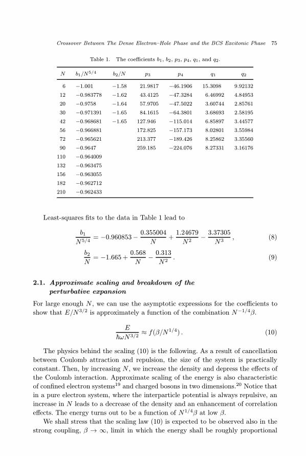
Table 1. The coefficients b1, b2, p3, p4, q1, and q2.

N b1/N5/4 b2/N p3 p4 q1 q2

6 −1.001 −1.58 21.9817 −46.1906 15.3098 9.92132

12 −0.983778 −1.62 43.4125 −47.3284 6.46992 4.84953

20 −0.9758 −1.64 57.9705 −47.5022 3.60744 2.85761

30 −0.971391 −1.65 84.1615 −64.3801 3.68693 2.58195

42 −0.968681 −1.65 127.946 −115.014 6.85897 3.44577

56 −0.966881 172.825 −157.173 8.02801 3.55984

72 −0.965621 213.377 −189.426 8.25862 3.35560

90 −0.9647 259.185 −224.076 8.27331 3.16176

110 −0.964009

132 −0.963475

156 −0.963055

182 −0.962712

210 −0.962433

Least-squares fits to the data in Table 1 lead to

b1

N5/4= −0.960853− 0.355004

N+

1.24679

N2− 3.37305

N3, (8)

b2

N= −1.665 +

0.568

N− 0.313

N2. (9)

2.1. Approximate scaling and breakdown of the

perturbative expansion

For large enough N , we can use the asymptotic expressions for the coefficients to

show that E/N3/2 is approximately a function of the combination N−1/4β.

E

~ωN3/2≈ f(β/N1/4) . (10)

The physics behind the scaling (10) is the following. As a result of cancellation

between Coulomb attraction and repulsion, the size of the system is practically

constant. Then, by increasing N , we increase the density and depress the effects of

the Coulomb interaction. Approximate scaling of the energy is also characteristic

of confined electron systems19 and charged bosons in two dimensions.20 Notice that

in a pure electron system, where the interparticle potential is always repulsive, an

increase in N leads to a decrease of the density and an enhancement of correlation

effects. The energy turns out to be a function of N1/4β at low β.

We shall stress that the scaling law (10) is expected to be observed also in the

strong coupling, β → ∞, limit in which the energy shall be roughly proportional



to the energy of N independent excitons,

E

~ω

∣∣∣∣β→∞

= a0β2 + · · · , (11)

where a0 ≈ −N . The right hand side of Eq. (11) may thus be written as

N3/2(−β2/N1/2). The variational results of the next sections also support the scal-

ing behaviour (10).

A naive estimation of the convergence radius for the series (2) gives β < βc =

b1/b2. This estimation may be obtained formally as the pole of the Pade approxi-

mant

P1,1(β) = b0 +b1β

1 + q1β, q1 = −b2/b1 , (12)

which reproduces the expansion (2) for small β values. Notice the high-N asymp-

totic behaviour, βc ∼ 0.58 N1/4. βc gives an estimate for the density at which exci-

ton effects become important. Indeed, the density in our units is ρ ≈ N/(π〈r2〉) ≈3 N1/2/(2π), thus βc may be expressed in terms of ρ. Turning back to ordinary

units, we get a critical density, ρc ∼ 1/0.24πa2B, i.e. approximately four times the

close-packing density of excitons, 1/πa2B. This fact is consistent with the belief that

screening is less effective in two dimensions. Below ρc, exciton effects shall dominate

the quantum dynamics. As will be seen, ρc is also at the onset of pairing in the

BCS estimate of the next sections.

In the following sections, we will perform variational estimations expected to be

valid when pairing is not so strong, that is in the regime β/N1/4 ≤ 1.

3. Variational Estimations

Let us turn to the variational calculations. The simplest variational estimation one

can try is first-order perturbation theory.

E

~ω< EPT1(β) = b0 + b1β . (13)

This estimate may be improved by introducing a frequency, Ω, as an additional

variational parameter, i.e. by taking as trial function the product of two Slater

determinants of harmonic-oscillator states with a frequency Ω. The result is,

E

~ω< min

Ω

1

2(Ω + 1/Ω)EPT1

(2√

Ω

Ω + 1/Ωβ

). (14)

We checked that the result coming from (14) practically coincides with the

Hartree–Fock (HF) energy for this system.11 Thus, we will call (14) the HF estimate.

The mechanism by which the energy is lowered is pairing. We may take account

of it with the help of a BCS-like wave function.21 This may be a good estimation



for weak pairing, when correlations are not so strong. In the β axis, it means

β/N1/4 < 1. The wave function is given by

|BCS 〉 =

Nmax∏j=1

(uj + vjh+j e

+j′) |0〉h |0〉e . (15)

h+j and e+

j are hole and electron (harmonic oscillator) creation operators acting

on their respective vacua |0〉h and |0〉e. j = (k, l, sz) is a composed index, j′ =

(k,−l,−sz). sz is the spin projection. vj and uj are normalised according to u2j +

v2j = 1. The total angular momentum corresponding to |BCS 〉 is zero because the

angular momentum of each pair is zero. The mean value of the total electron (hole)

spin may be forced to be zero by requiring v(k, l, sz) = v(k, l,−sz). Thus, vj does

not depend on sz and we can write vn instead of vj .

|BCS 〉 is not an eigenfunction of the particle number operator. In a finite system,

we shall project onto the state with the correct number of particles. This will be done

in two steps: first, an approximate projection before variation over the parameters

vn entering the BCS function (the Lipkin–Nogami scheme,8) and then an exact

Monte Carlo projection of the BCS function onto the sector with N pairs.9

3.1. The Lipkin-Nogami estimate

In the Lipkin–Nogami (LN) method,8 one assumes an approximate polynomial

dependence of H on the particle number operator N ,

H = λ0 + 2λ1N + λ2N2 . (16)

By taking expectation values of H over exact and BCS functions and comparing

results, we arrive to

ELN = EBCS − 2λ1(〈N〉BCS −N)− λ2(〈N2〉BCS −N2) , (17)

where

EBCS = 〈H〉BCS =∑n

4εn − 2β

⟨n, n

∣∣∣∣1r∣∣∣∣n, n⟩ v2

n

− 2β∑n1 6=n2

⟨n1, n2

∣∣∣∣1r∣∣∣∣n2, n1

⟩v2n1v2n2

+ vn1un1vn2un2 . (18)

Minimization over λ1 leads to

N =

⟨∑j

e+j ej

⟩BCS

=

⟨∑j

h+j hj

⟩BCS

= 2∑n

v2n . (19)



The equation of minimum with respect to the vn can be written in the form of

standard gap equations

∆n = β∑n1 6=n

⟨n, n1

∣∣∣∣1r∣∣∣∣n1, n

⟩∆n1

2√

∆2n1

+ (εHFn1− µ)2

(20)

where the HF energies are given by

εHFn = εn −

β

2

⟨n, n

∣∣∣∣1r∣∣∣∣n, n⟩− β ∑

n1 6=n

⟨n, n1

∣∣∣∣1r∣∣∣∣n1, n

⟩v2n1− λ2(N − v2

n) , (21)

and we used the common BCS parametrization

v2n =

1

2

(1− εHF

n − µ√∆2n + (εHF

n − µ)2

). (22)

The chemical potential, µ = λ1 + λ2/2 was introduced in Eq. (22). For the

determination of λ2, the system of equations

〈H − λ0 − 2λ1N − λ2N2〉BCS = 0 , (23)

〈(H − λ0 − 2λ1N − λ2N2)N〉BCS = 0 , (24)

〈(H − λ0 − 2λ1N − λ2N2)N2〉BCS = 0 , (25)

is used.8 It makes the LN method not throughly variational. The first equation

determines the constant λ0. The second turns to be equivalent to the gap equation

(20). For λ2, we get

λ2 =a1a5 − a2a4

a3a5 − a22

, (26)

where

a1 = 〈HN2〉BCS − 〈H〉BCS〈N2〉BCS , (27)

a2 = 〈N3〉BCS −N〈N2〉BCS (28)

a3 = 〈HN4〉BCS − 〈N2〉2BCS , (29)

a4 = 〈HN〉BCS −N〈H〉BCS , (30)

a5 = 〈N2〉BCS −N2 . (31)

The resulting equations were solved iteratively starting from εHFn = εn, ∆n =

0.2. First, the explicit expressions for v2n are used and the nonlinear equation (19) is

solved for µ. After that, we obtain λ2 from (26), and the ∆n and εHFn are recalculated

from (20) and (21). The process is repeated until the variation in any of the εHFn is

less than 10−10.

Calculations were carried out for 6 ≤ N ≤ 90 pairs and a maximum of 600

one-particle states for both electrons and holes (i.e. 300 orbitals, because there are

2 spin states for each orbital). The absolute error in computing Coulomb matrix



elements is less than 10−8. As is Eq. (14), we introduced an additional parameter

Ω, and used the inequality

E ≤ min

Ω

1

2(Ω + 1/Ω)ELN

(2Ω1/2

Ω + 1/Ωβ

), (32)

where ELN is the result from Eq. (17) at Ω = 1. The variation of Ω can be thought

of as a simplified self-consistent Hartree–Fock–Bogoliubov procedure, in which the

mean field is forced to be a harmonic potential.

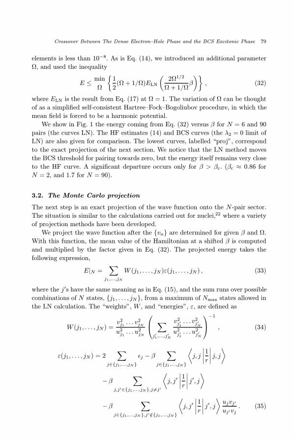
We show in Fig. 1 the energy coming from Eq. (32) versus β for N = 6 and 90

pairs (the curves LN). The HF estimates (14) and BCS curves (the λ2 = 0 limit of

LN) are also given for comparison. The lowest curves, labelled “proj”, correspond

to the exact projection of the next section. We notice that the LN method moves

the BCS threshold for pairing towards zero, but the energy itself remains very close

to the HF curve. A significant departure occurs only for β > βc. (βc ≈ 0.86 for

N = 2, and 1.7 for N = 90).

3.2. The Monte Carlo projection

The next step is an exact projection of the wave function onto the N -pair sector.

The situation is similar to the calculations carried out for nuclei,22 where a variety

of projection methods have been developed.

We project the wave function after the vn are determined for given β and Ω.

With this function, the mean value of the Hamiltonian at a shifted β is computed

and multiplied by the factor given in Eq. (32). The projected energy takes the

following expression,

E|N =∑

j1,...,jN

W (j1, . . . , jN )ε(j1, . . . , jN ) , (33)

where the j′s have the same meaning as in Eq. (15), and the sum runs over possible

combinations of N states, j1, . . . , jN, from a maximum of Nmax states allowed in

the LN calculation. The “weights”, W , and “energies”, ε, are defined as

W (j1, . . . , jN ) =v2j1. . . v2

jN

u2j1. . . u2

jN

∑j′1,...,j

′N

v2j′1. . . v2

j′N

u2j′1. . . u2

j′N

−1

, (34)

ε(j1, . . . , jN ) = 2∑

j∈j1,...,jNεj − β

∑j∈j1,...,jN

⟨j, j

∣∣∣∣1r∣∣∣∣ j, j⟩

− β∑

j,j′∈j1,...,jN,j 6=j′

⟨j, j′

∣∣∣∣1r∣∣∣∣ j′, j⟩

− β∑

j∈j1,...,jN,j′ /∈j1,...,jN

⟨j, j′

∣∣∣∣1r∣∣∣∣ j′, j⟩ ujvj′

uj′vj. (35)



0 0.2 0.4 0.6 0.8 1 1.2 1.4 1.6 1.8β

−4

−2

0

2

4

6

8

10

12

14

16

18

20

Ene

rgy

HFBCSLNProj

(a)

0 0.5 1 1.5 2 2.5 3β

0

200

400

600

800

1000

1200

Ene

rgy

HFBCSLNProj

(b)

Fig. 1. (a) and (b): Ground-state energies of the 6-exciton and 90-exciton systems respectively.

The expression (33) for the projected energy allows a simple Monte Carlo eval-

uation, where the sets j1, . . . , jN are generated with probability W (j1, . . . , jN )

by means of a Metropolis algorithm.23 Other equivalent forms of Eq. (33), see for

example Ref. 24, are not suited for this evaluation. The procedure seems to be

particularly efficient in Nuclear Physics calculations as well.9

The results are also drawn in Fig. 1. The improvement is significant for β ∼ βc,

and its relative importance diminishes as N is increased.



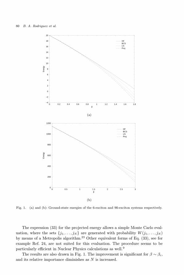
0 0.25 0.5 0.75 1 1.25β/N

1/4

−0.5

−0.25

0

0.25

0.5

0.75

1

1.25

1.5

E/N

3/2

6 particles12 particles20 particles30 particles42 particles56 particles72 particles90 particlesHF

Fig. 2. Scaling of the ground-state energies.

3.3. Results

We show in Fig. 2 our best results for the energies of the systems under study. The

scaled energies show a remarkable similarity. A significant pairing (i.e. departure

from the HF curve) is seen only for (β/N1/4) ≥ 0.55.

Finally, we give a parametrisation of the ground-state energy obtained from

the best of our variational estimates. The energy is written in the form of a Pade

approximant,25

Egs = b0 + b1β +b2β

2 + p3β3 + p4β

4

1 + q1β + q2β2, (36)

where p3 = q1p4/q2 − b1q2, and the coefficients p4, q1, and q2 are fitted from our

numerical results. The obtained values are shown in Table 1.

4. Concluding Remarks

We have studied electron–hole systems in quantum dots under strong and interme-

diate confinement, where the dense electron–hole or the BCS excitonic phases are

present.

The breakdown of perturbation theory and a significant pairing in the BCS wave

function, both take place at a density which is roughly four times the close-packing

density of excitons. We interpret this result as a crossover between the two phases.

As mentioned before, with an increase in β, particle correlations shall become

more and more important. We shall observe signals of the “excitonic”, “biexcitonic”,

etc. insulating phases. To obtain the true energies and wave functions of these

phases more powerful methods as, for example, the Green-function Monte Carlo

method23 should be applied. Even a variational Monte Carlo estimation, as that

one carried out for the homogeneous case in Ref. 26, may be biased by the chosen



trial functions. The density matrix renormalisation group method of Ref. 27 could

also be useful. This analysis requires a considerable amount of additional work

and is outside the scope of the present paper. On the other hand, there is another

very interesting question concerning the stability of the free system, i.e. whether it

remains bound after the external potential is switched off. We have some indications

that the two-dimensional triexciton and the four-exciton system are unbound12 (or

very weakly bound). But the situation may be analogous to nuclei, where there

is a small instability island around atomic number 5. Some of these problems are

currently under investigation.

Acknowledgments

The authors acknowledge support from the Colombian Institute for Science and

Technology (COLCIENCIAS). Part of this work was done during a visit of A. G.

and B. R. to the Abdus Salam ICTP under the Associateship Scheme and the

Visiting Young Student Programme.

References

1. See, for example, L. V. Keldysh in Bose–Einstein Condensation, eds. A. Griffin,D. W. Snoke and S. Stringari (Cambridge Univ. Press, 1995), p. 246, and referencestherein.

2. M. H. Anderson, J. R. Ensher and M. R. Mathews et al., Science 269, 198 (1995);K. B. Davis, M. O. Mewes and M. R. Andrews et al., Phys. Rev. Lett. 75, 3969 (1995);C. C. Bradley, C. A. Sackett, J. J. Tollet and R. G. Hulet, ibid. 75, 1687 (1995).

3. J. C. Kim and J. P. Wolfe, Phys. Rev. B57, 9861 (1998).4. V. Negoita, D. W. Snoke and K. Eberl, Phys. Rev. B60, 2661 (1999).5. G. Bastard and B. Gil (eds.), Optics of excitons in confined systems, Journal de

Physique IV, Vol. 3, Colloque C 3 (1993).6. R. Ambigapathy, I. Bar-Joseph, D. Y. Oberli et al., Phys. Rev. Lett. 78, 3579 (1997).7. E. Dekel, D. Gershoni, E. Ehrenfreund, D. Spektor, J. M. Garcia and P. M. Petroff,

Phys. Rev. Lett. 80, 4991 (1998); E. Dekel, D. Gershoni, E. Ehrenfreund, J. M. Garciaand P. M. Petroff, cond-mat/9904334.

8. H. C. Pradham, Y. Nogami and J. Law, Nucl. Phys. A201, 357 (1973); J. Dobaczewskiand W. Nozarewickz, Phys. Rev. C47, 2418 (1993).

9. R. Capote and A. Gonzalez, Phys. Rev. C59, 3477 (1999).10. M. Rho and J. O. Rasmussen, Phys. Rev. 135, B1295 (1964).11. A. Gonzalez, R. Capote, A. Delgado and L. Lavin, cond-mat/9809399, submitted.12. R. Perez and A. Gonzalez, submitted.13. J. Speth (ed.), Electric and Magnetic Giant Resonances in Nuclei (World Scientific,

Singapore, 1991).14. J. P. Connerade (ed.), Correlations in Clusters and Related Systems (World Scientific,

Singapore, 1996).15. A. de Shalit and H. Feschbach, Theoretical Nuclear Physics Vol. I, (John Wiley, New

York, 1974).16. R. Cote and A. Griffin, Phys. Rev. B37, 4539 (1988).17. A. Wojs, P. Hawrylak, S. Fafard and L. Jacak, Phys. Rev. B54, 5604 (1996).18. C. M. Bender and S. A. Orszag, Advanced Mathematical Methods for Scientists and

Engineers (McGraw-Hill, New York, 1978).



19. A. Gonzalez, B. Partoens and F. M. Peeters, Phys. Rev. B56, 15740 (1997).20. A. Gonzalez, B. Partoens, A. Matulis and F. M. Peeters, Phys. Rev. B59, 1653 (1999).21. C. P. Enz, A course on Many-Body Theory Applied to Solid State Physics (World

Scientific, 1992).22. D. C. Zheng, D. W. L. Sprung and H. Flocard, Phys. Rev. C46, 1355 (1992).23. D. M. Ceperley, in Spring College in Computational Physics, ICTP, Trieste, 1997.24. V. G. Soloviev, Theory of Complex Nuclei (Oxford, New York, 1976).25. L. Quiroga, F. J. Rodriguez and A. Gonzalez, Proceedings of ICPS-24, Jerusalem,

1998, in press.26. X. Zhu, M. S. Hybertsen and P. B. Littlewood, Phys. Rev. B54, 13575 (1996).27. J. Dukelsky and G. Sierra, Phys. Rev. Lett. 83, 172 (1999).

Crossover Between the Electron-Hole Phase and the BCS Excitonic Phase in Quantum Dots

Documents