Crossing the Line: Crowd Counting by Integer Programming with Local Features Zheng Ma Antoni B. Chan Department of Computer Science City University of Hong Kong [email protected], [email protected] Abstract We propose an integer programming method for estimat- ing the instantaneous count of pedestrians crossing a line of interest in a video sequence. Through a line sampling process, the video is first converted into a temporal slice image. Next, the number of people is estimated in a set of overlapping sliding windows on the temporal slice image, using a regression function that maps from local features to a count. Given that count in a sliding window is the sum of the instantaneous counts in the corresponding time interval, an integer programming method is proposed to recover the number of pedestrians crossing the line of inter- est in each frame. Integrating over a specific time interval yields the cumulative count of pedestrian crossing the line. Compared with current methods for line counting, our pro- posed approach achieves state-of-the-art performance on several challenging crowd video datasets. 1. Introduction The goal of crowd counting is to estimate the num- ber of people in a region of interest (ROI counting), or passing through a line of interest (LOI counting) in video. Crowd counting has many potential real-world applications, including surveillance (e.g., detecting abnormally large crowds, and controlling the number of people in a region), resource management (counting the number of people en- tering and exiting), and urban planning (identifying the flow rate of people around an area). Beyond people, these counting methods can also be applied to other objects, such as animals passing through a particular boundary, blood cells flowing through a blood vessel under a microscope, and the rate of car traffic. Therefore crowd counting is a crucial topic in video surveillance and other related fields. However, it is still a challenging task because of several fac- tors: 1) in crowded scenes, occlusion between pedestrians is common, especially for large groups in confined areas; 2) the perspective of the scene causes people to appear larger and move faster when they are close to the camera. These problems are especially prominent in “high-angle” camera (a) (b) (c) Figure 1. Line counting example: a) crowd scene and line-of- interest; b) temporal slice of the scene; c) Flow-mosaicking [1] result where a large blob leads to a big jump in the cumulative count. In contrast, our method can predict instantaneous counts better, yielding a better cumulative prediction over time. views (where the camera looks down at an angle), which are typical of outdoor surveillance cameras. Most previous approaches [2–6] focus on solving the ROI counting problem, and are based on the counting- by-regression framework, where features extracted from the ROI are directly regressed to the number of people. By bypassing intermediate steps, such as people detection, which can be error-prone on large crowds with severe oc- clusion, these counting-by-regression methods achieve ac- curate counts even on sizable crowds. In this paper, we focus on LOI counting, which has received relatively less attention so far. The goal of LOI counting is to count the number of people crossing a line (or visual gate) in the video (see Fig. 1a for example). In particular, the aim is to estimate both the cumulative count, i.e., the total count since the start of the video, and the instantaneous count, i.e., the count at any particular time or short temporal window. A naive approach to LOI counting is to apply ROI counting on the regions on each side of the LOI, and take the count difference. However, this LOI count will be erroneous when people enter and exit the ROIs at the same time, since the number of people in the regions remains the same. Current state-of-the-art LOI counting approaches (e.g. [1]) are based on extracting and counting crowd blobs from 2537 2537 2539

Welcome message from author
This document is posted to help you gain knowledge. Please leave a comment to let me know what you think about it! Share it to your friends and learn new things together.
Transcript

Crossing the Line: Crowd Counting by Integer Programming with Local Features
Zheng Ma Antoni B. Chan
Department of Computer Science
City University of Hong Kong
[email protected], [email protected]
Abstract
We propose an integer programming method for estimat-
ing the instantaneous count of pedestrians crossing a line
of interest in a video sequence. Through a line sampling
process, the video is first converted into a temporal slice
image. Next, the number of people is estimated in a set of
overlapping sliding windows on the temporal slice image,
using a regression function that maps from local features
to a count. Given that count in a sliding window is the
sum of the instantaneous counts in the corresponding time
interval, an integer programming method is proposed to
recover the number of pedestrians crossing the line of inter-
est in each frame. Integrating over a specific time interval
yields the cumulative count of pedestrian crossing the line.
Compared with current methods for line counting, our pro-
posed approach achieves state-of-the-art performance on
several challenging crowd video datasets.
1. Introduction
The goal of crowd counting is to estimate the num-
ber of people in a region of interest (ROI counting), or
passing through a line of interest (LOI counting) in video.
Crowd counting has many potential real-world applications,
including surveillance (e.g., detecting abnormally large
crowds, and controlling the number of people in a region),
resource management (counting the number of people en-
tering and exiting), and urban planning (identifying the
flow rate of people around an area). Beyond people, these
counting methods can also be applied to other objects, such
as animals passing through a particular boundary, blood
cells flowing through a blood vessel under a microscope,
and the rate of car traffic. Therefore crowd counting is a
crucial topic in video surveillance and other related fields.
However, it is still a challenging task because of several fac-
tors: 1) in crowded scenes, occlusion between pedestrians
is common, especially for large groups in confined areas; 2)
the perspective of the scene causes people to appear larger
and move faster when they are close to the camera. These
problems are especially prominent in “high-angle” camera
(a) (b)
(c)
� �� ��� ��� ��� ��� ����
��
��
��
���� ����
����
����
���
� � ����������� �
����������������� �������
Figure 1. Line counting example: a) crowd scene and line-of-
interest; b) temporal slice of the scene; c) Flow-mosaicking [1]
result where a large blob leads to a big jump in the cumulative
count. In contrast, our method can predict instantaneous counts
better, yielding a better cumulative prediction over time.
views (where the camera looks down at an angle), which are
typical of outdoor surveillance cameras.
Most previous approaches [2–6] focus on solving the
ROI counting problem, and are based on the counting-
by-regression framework, where features extracted from
the ROI are directly regressed to the number of people.
By bypassing intermediate steps, such as people detection,
which can be error-prone on large crowds with severe oc-
clusion, these counting-by-regression methods achieve ac-
curate counts even on sizable crowds. In this paper, we
focus on LOI counting, which has received relatively less
attention so far. The goal of LOI counting is to count the
number of people crossing a line (or visual gate) in the
video (see Fig. 1a for example). In particular, the aim is
to estimate both the cumulative count, i.e., the total count
since the start of the video, and the instantaneous count, i.e.,
the count at any particular time or short temporal window.
A naive approach to LOI counting is to apply ROI counting
on the regions on each side of the LOI, and take the count
difference. However, this LOI count will be erroneous when
people enter and exit the ROIs at the same time, since the
number of people in the regions remains the same.
Current state-of-the-art LOI counting approaches (e.g.
[1]) are based on extracting and counting crowd blobs from
2013 IEEE Conference on Computer Vision and Pattern Recognition
1063-6919/13 $26.00 © 2013 IEEE
DOI 10.1109/CVPR.2013.328
2537
2013 IEEE Conference on Computer Vision and Pattern Recognition
1063-6919/13 $26.00 © 2013 IEEE
DOI 10.1109/CVPR.2013.328
2537
2013 IEEE Conference on Computer Vision and Pattern Recognition
1063-6919/13 $26.00 © 2013 IEEE
DOI 10.1109/CVPR.2013.328
2539

���
� ���� �������
��
� ���� �������
Figure 2. Results of instantaneous count estimation on: a) UCSD and b) LHI datasets. The image is a temporal-slice of the video on the
LOI. The red and blue segments correspond to crowds moving in different directions, and the instantaneous count estimates appear above
and below the image.
a temporal slice of the video (e.g., the y-t slice of the video
volume). However, there are several drawbacks of these
“blob-centric” methods: 1) because the blob is not counted
until it has completely crossed the line, large blobs (e.g.,
containing more than 10 people) yield big jumps in the
cumulative count, which leads to poor instantaneous count
estimates (see Fig. 1c); 2) the counts in these large blobs
are not accurate, due to severe occlusion [1]; 3) current
evaluation methods for blob-based methods are based on
the ground-truth people in the blob, not the actual people
passing the line – hence, it is difficult to assess errors due to
segmentation failure of the blob. Moreover, these methods
typically require spatial-temporal normalization to handle
the differences in pedestrian size due to the camera perspec-
tive and pedestrian velocity. Current perspective normaliza-
tion methods [2, 7] require marking a reference person in
different positions in the video. For arbitrary videos (e.g.,
from the internet), these normalization techniques cannot be
applied if no suitable reference exists.
To address the above problems, we propose a novel
line counting algorithm that estimates instantaneous peo-
ple counts using local-level features and regression without
perspective normalization (see Fig. 2 for examples). The
contributions of this paper are three-fold. First, to overcome
the drawbacks of “blob-centric” methods, we propose an in-
teger programming approach to estimate the instantaneous
counts on the LOI, from a set of ROI counts in the tempo-
ral slice image. The cumulative counts of our method are
smoother and more accurate than “blob-centric” methods.
Second, we introduce a novel local histogram-of-oriented-
gradients (HOG) feature, which is robust to the effects of
perspective and velocity and yields accurate counts even
without spatial-temporal normalization. Third, we demon-
strate experimentally that our method can achieve state-of-
the-art results for both cumulative and instantaneous LOI
counts on two challenging datasets.
2. Related work
Counting-by-regression methods focus on either count-
ing people in a region-of-interest (ROI), or counting people
passing through a line-of-interest (LOI). For ROI counting,
features are extracted from each crowd segment in an im-
age, and a regression function maps between the feature
space and the number of people in the segment. Typically
low-level global features are extracted from the crowd seg-
ment, internal edges, and textures [1, 2, 4, 6]. The seg-
ment area is a prototypical feature that can indicate the total
number of pedestrians in the segment. [2] shows that there
is a near linear relationship between the segment area and
the number of pedestrian, as long as the feature extraction
process properly weights each pixel according to the per-
spective of the scene. [2] also provides a method to generate
a perspective map, by manually labeling a reference person
at opposite positions in the scene. Low-level features can
also be extracted from each crowd blob, i.e., an individual
connected-component in the segment, which contains sever-
al pedestrians [5, 6]. Regression methods include Gaussian
process regression [8] or Bayesian Poisson regression [4],
which are both kernel methods that can estimate non-linear
functions. [9] proposes an alternative approach to ROI
counting, using pixel-wise density learning. The crowd
density at each pixel is regressed from the feature vector,
and the number of pedestrians in a ROI is obtained by inte-
grating over the crowd density map.
Line-of-interest (LOI) counting essentially estimates the
number of people in a temporal-slice image (e.g., the y-t
slice of the video volume), the result of which represents
the number of people passing through the line within that
time window. However, with the basic temporal slice,
people moving at fast speeds will have fewer pixels than
253825382540

those moving slowly, thus confounding the regression func-
tion. The flow-mosaiking framework [1] corrects for this by
changing the thickness of the line, based on the the average
velocity of the pixels in the crowd blob, resulting in a “flow
mosaic”. [7] is used for perspective normalization, and the
count in each blob is estimated from low-level features. The
blob count can only be estimated after the blob has passed
the line, and hence large jumps in the cumulative count
can occur, and instantaneous counts (indicating when each
person passes the line) are not possible. In contrast to [1],
our proposed approach performs ROI counting on windows
in the temporal slice image, and uses integer programming
to recover the instantaneous count on the line.
For both ROI and LOI counting, global- and blob-
level features are very sensitive to the perspective (spatio-
temporal) normalization, especially in scenes with large
depth changes. In our experiments, the accuracy of counting
using low-level features drops significantly without normal-
ization, whereas the accuracy using our local HOG feature
remains at a similar level. [9] also uses local features, based
on random forest [9] or SIFT features [10], but still requires
perspective normalization.
Finally, counting can also be performed using people
detection methods [11–13], which are based on “individual-
centric” features, i.e., features describing the whole per-
son, such as the HOG descriptor of a whole person [11].
The deformable part-based model (DPM) [13] also builds a
HOG descriptor of a whole person, by using a more flexible
layout model for the spatial relationship between HOG parts
at different scales. While this results in a model that is
better adapted to varying poses of a single person, it still has
problems in detecting partially-occluded people in groups.
In contrast, by removing the layout model, our local HOG
representation is better able to handle occlusions.
3. Local HOG feature
Fig. 3a shows an example of a temporal-slice image with
a sizable crowd walking in two directions. Due to the cam-
era tilt angle, which is nearly 45 degree, the occlusion of
pedestrians is heavy. The torsos or the legs of the occluded
pedestrians are not visible in most cases. Hence, the st-
andard histogram-of-oriented-gradients (HOG) feature and
detector [11] will not work well in this scenario. In this
paper, we propose a local HOG descriptor for crowd count-
ing. In contrast to the standard HOG, which is a descriptor
of a whole person, the local HOG can describe parts of
the person independently. As a result, in crowded scenes,
meaningful descriptors can still be extracted from partially-
occluded people.
3.1. Local HOG descriptor
We define a local HOG descriptor as one “block” of
the standard HOG feature, extracted from a 8×8 image
(a) (b)
(c)
� �� �� �� ���
��
��
��
������� ���
����
����!�
Figure 3. Examples of local HOG features: a) temporal-slice im-
age; b) image patches and their local HOG features; c) one bin of
the bag-of-words histogram versus crowd size.
patch. Each block contains four 4×4 “spatial cells”, from
which the local histogram of oriented gradients is extracted.
Fig. 3b presents examples of the local HOG features extract-
ed from a crowd in the temporal slice image. Note how the
local HOG feature can represent the head-shoulders, side,
or legs and feet of a person. We also considered rectangular
image patches (e.g., 8×16) and other sizes, and found that
the 8×8 image patches yield the best performance in the ex-
periments. Finally, we considered applying a weight to the
gradient magnitudes using a spatial Gaussian kernel (similar
to the SIFT descriptor [10]), but this did not increase the
counting accuracy.
3.2. Global descriptor of local HOG features
The number of extracted local HOG features depends
on the size of the crowd segments in each video frame,
with potentially hundreds of local features extracted per
frame due to dense sampling. Hence, further processing
is required to summarize the set of local features into a
concise feature vector, which describes the crowd. The set
of local HOG features is summarized with a bag-of-words
histogram, where each bin represents the number of times
a local HOG codeword appears in the image. Fig. 3c plots
the value of one bin of the histogram versus the number of
people in the crowd segment. The bin value varies linearly
with the number of people, which suggests that the bag-
of-words of local HOG can be a suitable feature for crowd
counting. Finally, we do not apply histogram normalization
methods (e.g., TF, TF-IDF). Normalization will obfuscate
the absolute number of codewords in the segment, making
histograms from large crowds similar to those from small
crowds, which confounds the regression function.
4. Line counting framework
In this section, we propose our line counting framework,
which is illustrated in Fig. 4. Given an input video se-
quence, the video is first segmented into crowds of interest,
e.g., corresponding to people moving in different directions.
253925392541

����������
���
����������� �����������������������
����������������
�������������������������������
����������������������������������
���������������������������������
Figure 4. The proposed line counting framework.
A temporal slice image and temporal slice segmentation are
formed by sampling the LOI over time. Next, a sliding
window is placed over the temporal slice, forming a set of
temporal ROIs. Features are extracted from each temporal
ROI, and the number of people in each ROI is estimated us-
ing a regression function. Finally, an integer programming
approach is used to recover the instantaneous count from
the set of temporal ROI counts.
4.1. Crowd segmentation
Motion segmentation is first applied to the video to focus
the counting algorithm on different crowds of interest (e.g.,
moving in opposite directions). We use a mixture of dynam-
ic textures motion model [14] to extract the regions with dif-
ferent crowd flows. The video is divided into a set of spatio-
temporal video cubes, from which a mixture of dynamic
textures is learned using the EM algorithm [14]. The motion
segmentation is then formed by assigning video patches
to the most likely dynamic texture component. Static or
very slow moving pedestrians will not be included in the
motion segmentation, which is desirable, since the counting
algorithm should ignore people who have stopped on the
line, in order to avoid double counting.
4.2. Line sampling and temporal ROI
In contrast to flow-mosaicking [1], we use line sampling
with a fixed line-width to obtain the temporal slice image.
As shown in Fig. 4, the input video image and its corre-
sponding segmentation are sampled at the same line per
�������
Figure 5. Temporal slices of pedestrians with different velocities.
��
�� ��� ��� ��� ��� ��� ��� ���
��
��
"�
#�
(b)
�� ��� ��� ��� ��� ��� ��� ���
��
��
"�
#� �$��$��$"�$#��$�
(c)
�� ��� ��� ��� ��� ��� ��� ���
��
��
"�
#� �
�$�
�$�
Figure 6. a) temporal-slice image, and its b) temporal and c) spatial
weighting maps.
frame. The sampled image slices and segment slices are
collected to form the temporal slice image and temporal
slice segmentation, where each column in the slice image
corresponds to the LOI at a given time. To obtain the tem-
poral ROIs, a sliding window is moved horizontally across
the slice image, using a stepsize of one pixel.
4.3. Feature extraction
Features are extracted from each crowd segment in each
temporal ROI. In this paper, we consider both low-level
global features and local features. We use the 30 global
features from [3], which measure various properties of the
segment, and its internal edges and texture (see Table 1).
For the local features, we use our proposed local HOG
features and bag-of-words model. A set of local HOG
features is extracted from densely sampled patches over
the crowd segment in the temporal ROI. The set of local
HOGs is then summarized using the bag-of-words model,
as described in Section 3, resulting in a single feature vector
for each crowd segment for each ROI.
4.4. Spatial-temporal normalization
Because the temporal slice image is generated using a
fixed-width line, the width of a person will change with its
velocity. In particular, people moving slowly across the LOI
will appear wider than those moving fast, as illustrated in
Fig. 5. Hence, temporal normalization is required during
254025402542

Table 1. Spatial-temporal normalization for low level features.
Group Features Dimension Weighting strategy
area 1 wpwv
segment perimeter 1√wpwv
features perimeter-area ratio 1√wpwv
(10) perimeter edge orientation 6
√w2
p cos2 θ + w2
v sin2 θ
blob number 1 N/A
edge edge length 1√wpwv
features edge orientation 6
√w2
p cos2 θ + w2
v sin2 θ
(8) edge Minkowski 1√wpwv
texture texture homogeneity 4√wpwv
features texture energy 4√wpwv
(12) texture entropy 4√wpwv
feature extraction to adjust for the speed of the person (fea-
tures). A temporal weight map wv(x, y) is formed from the
tangent velocity of each LOI pixel, estimated with optical
flow [15] (see Fig. 6b). Faster moving people have higher
weights, since their features will be present for less time.
In addition to the temporal normalization, the features
must also be normalized to adjust for perspective effects of
the angled camera. We follow [2] to generate the spatial
perspective weight map wp(x, y) (see Fig. 6c).
Both weighting maps are applied when extracting low-
level features from the image, yielding a spatio-temporal
normalization summarized in Table 1. For the area feature,
each pixel is weighted by wpwv , and for most edge and
texture features, the weighting of√wpwv is applied on
each pixel. The edge orientation features are sensitive to
a particular edge angle θ ∈ {0◦, 30◦, 60◦, 90◦, 120◦, 150◦},
and hence a weight of
√w2
p cos2 θ + w2
v sin2 θ is used to
readjust the contributions between wv and wp. For example,
when the edge is oriented horizontally (θ = 90◦), only the
temporal weight is applied, since there is no component of
the edge in the spatial direction.
For the local HOG feature, we resize the image patch by
scaling the height and width by wp and wv . This normalizes
the local HOG feature extraction to a common reference
size. However, normalization of the local HOG features
is not necessary; our experimental results show similar
performance between local HOG with and without spatio-
temporal normalization, which indicates the robustness of
the feature to perspective and velocity variations.
Finally, note that flow mosaicking [1] performs temporal
normalization by sampling the LOI using a variable line-
width, where the current width is based on the average
speed of the crowd blob. Because the same line-width must
be applied to the whole blob, blobs containing both fast and
slow people will not be normalized correctly. In contrast
to [1], we use a fixed line-width and per-pixel temporal
normalization, which can better handle large crowd blobs
with people moving at different speeds (e.g., in Figs. 6a
and 6b).
4.5. Count Regression
For each temporal ROI, the count in each crowd segment
of the ROI is predicted using a regression function that
directly maps between the feature vector (input) and the
number of people in the crowd segment (output). Gaussian
process regression (GPR) [8] has shown promising results
for the people counting task [2]. However, pedestrian
counts are discrete non-negative integer values, and hence
it is not suitable to use GP regression, which models con-
tinuous real-valued outputs. Aiming to take full advantage
of Bayesian inference, we use Bayesian Poisson regression
[3], which directly learns a regression function with discrete
integer outputs. We use the combination of RBF kernel
and linear kernel, which yielded the best performance, com-
pared to the single RBF kernel, linear, Bhattacharyya, his-
togram intersection, and Chi-squared-RBF kernels. Fig. 7a
presents an example of the predicted counts for the temporal
ROIs, along with the ground-truth.
4.6. Instantaneous count estimation
In the final stage, the instantaneous counts on the LOI are
recovered from the temporal ROI counts using an integer
programming formulation. The ith temporal ROI spans
time i through i + L − 1, where L is the width of the ROI.
Let ni be the count in the ith temporal ROI, and sj be the
instantaneous count on the LOI at time j. The temporal ROI
count ni is the sum of the instantaneous counts sj , within
the temporal window of the ROI,
ni = si + si+1 + · · ·+ si+L−1 =
L−1∑k=0
si+k, (1)
Defining the vector of ROI counts n = [n1, . . . , nN ]T and
s = [s1, . . . , sM ]T , where N is the number of temporal
ROIs and M is the number of video frames, we have
n = As, (2)
where A ∈ {0, 1}N×M is an association matrix with entries
aij =
{1, j ≤ i < j + L
0, otherwise.(3)
Both n and A are known, and hence finding s is a signal re-
construction problem, with non-negative integer constraints
on the counts sj . We propose to recover the instantaneous
counts s using an integer programming problem with a sum-
squared reconstruction error
s∗ =argmins
‖As− n‖2 s.t. sj ∈ Z+, ∀j, (4)
where Z+ is the set of non-negative integers. We solve (4)
using the optimization toolbox [16]. Fig. 7b presents an ex-
ample of the instantaneous counts recovered from the ROI
254125412543

(a) (b)
� ��� ��� "�� #�� �����
�
��
��
��
���� ����
����
����
���
� � ���������
���� �������
� ��� �����
�$�
�
�$�
�
�$�
���� ����
����
����
���
� � ���������
���� �������
(c) (d)
� ��� ����%�
�
�
�
���� ����
����
����
���
� � ���������
���� �������
� ��� �����
�$�
�
�$�
�
�$�
���� ����
����
����
���
� � ���������
���� �������
Figure 7. a) temporal ROI counts over time, and the recovered
instantaneous count estimates using b) integer programming, c)
least-squares, and d) non-negative least-squares.
counts in Fig. 7a with integer programming. The predicted
instantaneous counts are close to the ground-truth people
crossing the line.
Another possible solution is to relax the non-negative
integer constraints on sj . Letting sj be a real number, we
obtain a standard least-squares formulation, with s = A†n,
where A† is the pseudo-inverse of A. However, the recov-
ered sj will be both positive and negative, which are not in-
terpretable as counts (see Fig. 7c). Enforcing a non-negative
real constraint, sj ≥ 0, yields a non-negative least-squares
problem, with the recovered sj more similar to counts (see
Fig. 7d). However, this method causes localization errors,
where a single count is split into several small real-valued
counts in its neighborhood (see arrow in Fig. 7d). Using the
integer programming formulation fixes these localization
problems (Fig. 7b arrow).
5. Experiments
In this section, we present experimental results on using
the proposed LOI algorithm on two crowd datasets.
5.1. Pedestrian datasets
We consider two datasets in our experiments, the UCSD
people counting dataset [2] and the LHI pedestrian dataset
[17]. An example frame from the UCSD dataset is shown in
Fig. 8a. The video is captured by a stationary digital cam-
corder with an angled viewpoint over a walkway at UCSD.
The dataset contains 2000 video frames, with a frame size
of 238 × 158 and frame rate of 10 fps. The LHI dataset
contains three types of video, categorized by the camera
tilt angle. In our experiments, we use the 3-3 video with
40 degrees camera tilt angle, which is the most challenging
video in LHI due to the large amounts of occlusion. An
example frame is displayed in Fig. 8b. The 3-3 video has
frame size 352× 288.
(a)
64 [64]
35 [34](b)
58 [61]
0 [0]
Figure 8. Examples of input video with line position for a) UCSD
dataset, and b) video 3-3 of LHI dataset.
5.2. Experimental setup
For the UCSD dataset, we follow the experimental pro-
tocol in [2], where the training set consists of 800 frames
(frames 600 to 1399), and the remaining 1200 frames are
used as the test set for validation. For the LHI dataset, the
training set is the first 800 frames and the following 1200
frames are the test set. The LOI positions are also shown
in Fig. 8. For UCSD, the crowd was separated into two
components moving in opposite directions on the walkway
(right and left), using the method described in Section 4.1.
For LHI, the crowd is only moving in the right direction.
We estimate the instantaneous and cumulative counts on
the LOI using our proposed framework. The length of the
sliding window is 238 pixels. We tested both the global low-
level features [2, 4] and the proposed local HOG features,
with and without using spatio-temporal normalization. The
regression model is learned from the training set (UCSD
or LHI), and predictions made on the corresponding test
set. For comparison, we also predict the cumulative counts
using the flow-mosaicking algorithm [1]. Both methods
are run on the same motion segmentation and optical flow
images.
The cumulative counting results are evaluated with the
mean squared error (MSE) and the absolute error between
the predicted counts and the ground truth number of people,
averaged over all frames in the test set. For flow mosaick-
ing, which is blob-based and inherently cannot produce sm-
ooth cumulative counts, we also consider a “blob ground-
truth” that updates only when the predicted count changes,
i.e., when a blob is counted.
A recall-distance curve is used to measure the perfor-
mance of the instantaneous count predictions. The ground-
truth instantaneous count and the predictions are matched
pairwise using the Hungarian algorithm to find pairs with
minimal temporal distances (i.e., match the red stars with
blue lines in Fig. 11b). A recall-distance curve is formed by
sweeping a threshold distance d, and recording the fraction
of pairwise matches with distance less than d. The curve
represents the accuracy of detecting a person crossing the
line within duration d of the ground-truth crossing.
5.3. Experimental results
The cumulative counting results are summarized in
Table 2, with plots of the cumulative and instantaneous
254225422544

� �� �� �� �� �� "� &� #� '� ����
�$�
�$�
�$�
�$�
�$�
�$"
�$&
�$#
�$'
�
���� ��
���
�������%���� ��
()*+%,������ �%-����()*+%,������ �%.���()*+%.���%-����()*+%.���%.���.�/%.���%-����.�/%,������ �%-����
Figure 9. Recall-distance curves on UCSD and LHI datasets.
counts shown in Figs. 11-16. First comparing the different
feature sets on the UCSD dataset, the local HOG feature
achieves comparable results with the global low-level fea-
tures (0.6040 error vs 0.5342) for the left direction. On the
right direction, local HOG has significantly less error than
the global features (0.6883 vs 1.5067). Since the right di-
rections contains larger crowds, this suggests that the local
HOG features are better at counting the partially-occluded
people. Furthermore, the counting error for the local HOG
feature is nearly the same when no spatio-temporal normal-
ization is used, increasing slightly from 0.6050/0.6883 to
0.6083/0.7100. On the other hand, the error for the global
features increases significantly, e.g., from 1.5067 to 2.4158
for the right direction. This demonstrates that the local
HOG feature is robust to perspective and velocity effects,
whereas the global features are sensitive to these effects.
Our LOI counting framework using local HOG has low-
er error than flow-mosaicking (for both the ground-truth
and blob ground-truth). Flow-mosaicking has a particular-
ly large error (8.2400) on the right direction. In crowded
scenes with large blobs, the flow mosaicking method tends
to have high error, which is also shown in Fig. 14 and
Fig. 16. Similar results are obtained on the LHI video,
demonstrating that our framework achieves lower cumula-
tive counting error than flow-mosaicking.
The recovered instantaneous counts are presented in
Fig. 2, and the accuracy is evaluated using the recall-
distance curves in Fig. 9. On the UCSD dataset, our method
can correctly identify over 80% of the pedestrians crossing
the line within 2 seconds (20 frames, 10 fps), and on the
LHI dataset, almost 90% within 2 seconds (50 frames, 25
fps). Our method can generate more accurate instantaneous
counts than flow mosaicking, which is a “blob-centric”
method. For comparison, flow-mosaicking can identify
55% and 75% of the pedestrians within 2 seconds on UCSD,
and 72% on LHI.
Finally, Fig. 10a presents the average absolute count-
��� ��� ����
�
�
�
�
���
�� �������� �
���
���
����
�
��� ��� ����
��
��
��
��
�����
�� �������� �
���
���
����
()*+%,������ �%-����()*+%.���%-����()*+%,������ �%.���()*+%.���%.���.�/%.���%-����.�/%,������ �%-����
()*+%-����()*+%.���.�/%-����
Figure 10. Comparison over different time intervals: a) average
error vs interval width; b) average count vs interval width
ing error for varying time intervals (window lengths),
and Fig. 10b shows the corresponding average number of
ground truth people. For our method, the counting error is
relatively stable regardless of the interval width, whereas
that of flow-mosaicking increases as the interval width and
number of people increases. Two videos of our line count-
ing results on UCSD and LHI datasets can be found in the
supplemental material.
6. Conclusion
We present a novel line counting framework in this
paper, which is based on using integer programming to
recover the instantaneous counts on the LOI from ROI
counts on a sliding window over the temporal slice im-
age. We validate our framework on two challenging data-
sets. The results show that, compared with global low-level
features, the proposed local HOG feature is more robust
to the perspective and object velocity variations, and per-
forms equally well without using spatio-temporal normal-
ization. Moreover, compared with “blob-centric” methods
(e.g. flow-mosaicking), our method can generate more ac-
curate instantaneous and cumulative counts, especially in
crowded scenes.
Acknowledgments
The authors thank Yang Cong for the videos from the
LHI dataset [17]. This work was supported by the Research
Grants Council of the Hong Kong Special Administrative
Region, China [CityU 110610].
References
[1] Y. Cong, H. Gong, S.-C. Zhu, and Y. Tang, “Flow mosaicking: Real-
time pedestrian counting without scene-specific learning,” in CVPR,
2009, pp. 1093 –1100.
[2] A. B. Chan, Z.-S. J. Liang, and N. Vasconcelos, “Privacy preserv-
ing crowd monitoring: Counting people without people models or
tracking,” in CVPR, 2008, pp. 1 –7.
[3] A. B. Chan and N. Vasconcelos, “Counting people with low-level
features and bayesian regression,” IEEE Trans. on Image Processing,
vol. 21, no. 4, pp. 2160 –2177, 2012.
[4] ——, “Bayesian poisson regression for crowd counting,” in ICCV,
2009, pp. 545 –551.
254325432545
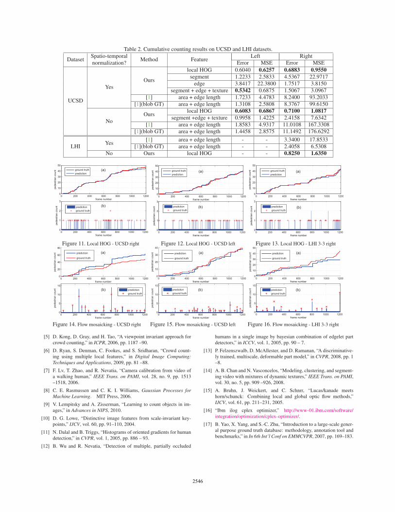
Table 2. Cumulative counting results on UCSD and LHI datasets.
DatasetSpatio-temporal
Method FeatureLeft Right
normalization? Error MSE Error MSE
UCSD
Yes
Ours
local HOG 0.6040 0.6257 0.6883 0.9550
segment 1.2233 2.5833 4.5367 22.9717
edge 3.8417 22.3800 1.7517 3.8150
segment + edge + texture 0.5342 0.6875 1.5067 3.0967
[1] area + edge length 1.7233 4.4783 8.2400 93.2033
[1](blob GT) area + edge length 1.3108 2.5808 8.3767 99.6150
No
Ourslocal HOG 0.6083 0.6867 0.7100 1.0817
segment +edge + texture 0.9958 1.4225 2.4158 7.6342
[1] area + edge length 1.8583 4.9317 11.0108 167.3308
[1](blob GT) area + edge length 1.4458 2.8575 11.1492 176.6292
LHIYes
[1] area + edge length - - 3.3400 17.8533
[1](blob GT) area + edge length - - 2.4058 6.5308
No Ours local HOG - - 0.8250 1.6350
� ��� ��� "�� #�� ���� �����
��
��
��
��
��
���� ����
����
����
���
� � ���� �������
���������
� ��� ��� "�� #�� ���� �����
�
�
�
���� ����
����
����
���
� � ���������
���� �������
01
0�1
Figure 11. Local HOG - UCSD right
� ��� ��� "�� #�� ���� �����
��
��
��
��
��
���� ����
����
����
���
� � ���� �������
���������
� ��� ��� "�� #�� ���� �����
�
�
�
���� ����
����
����
���
� � ���������
���� �������
01
0�1
Figure 12. Local HOG - UCSD left
� ��� ��� "�� #�� ���� �����
��
��
��
��
��
���� ����
����
����
���
� � ���� �������
���������
� ��� ��� "�� #�� ���� �����
�
�
�
���� ����
����
����
���
� � ���������
���� �������
01
0�1
Figure 13. Local HOG - LHI 3-3 right
� ��� ��� "�� #�� ���� �����
�
��
��
���� ����
����
����
���
� � ���������
���� �������
� ��� ��� "�� #�� ���� �����
��
��
"�
#�
���� ����
����
����
���
� � ���������
���� �������
01
0�1
Figure 14. Flow mosaicking - UCSD right
� ��� ��� "�� #�� ���� �����
�
��
��
���� ����
����
����
���
� � ���������
���� �������
� ��� ��� "�� #�� ���� �����
��
��
��
��
���� ����
����
����
���
� � ���������
���� �������
01
0�1
Figure 15. Flow mosaicking - UCSD left
� ��� ��� "�� #�� ���� �����
�
��
��
���� ����
����
����
���
� �
��������� ���� �������
� ��� ��� "�� #�� ���� �����
��
��
��
��
��
���� ����
����
����
���
� � ���������
���� �������
01
0�1
Figure 16. Flow mosaicking - LHI 3-3 right
[5] D. Kong, D. Gray, and H. Tao, “A viewpoint invariant approach for
crowd counting,” in ICPR, 2006, pp. 1187 –90.
[6] D. Ryan, S. Denman, C. Fookes, and S. Sridharan, “Crowd count-
ing using multiple local features,” in Digital Image Computing:
Techniques and Applications, 2009, pp. 81 –88.
[7] F. Lv, T. Zhao, and R. Nevatia, “Camera calibration from video of
a walking human,” IEEE Trans. on PAMI, vol. 28, no. 9, pp. 1513
–1518, 2006.
[8] C. E. Rasmussen and C. K. I. Williams, Gaussian Processes for
Machine Learning. MIT Press, 2006.
[9] V. Lempitsky and A. Zisserman, “Learning to count objects in im-
ages,” in Advances in NIPS, 2010.
[10] D. G. Lowe, “Distinctive image features from scale-invariant key-
points,” IJCV, vol. 60, pp. 91–110, 2004.
[11] N. Dalal and B. Triggs, “Histograms of oriented gradients for human
detection,” in CVPR, vol. 1, 2005, pp. 886 – 93.
[12] B. Wu and R. Nevatia, “Detection of multiple, partially occluded
humans in a single image by bayesian combination of edgelet part
detectors,” in ICCV, vol. 1, 2005, pp. 90 – 7.
[13] P. Felzenszwalb, D. McAllester, and D. Ramanan, “A discriminative-
ly trained, multiscale, deformable part model,” in CVPR, 2008, pp. 1
–8.
[14] A. B. Chan and N. Vasconcelos, “Modeling, clustering, and segment-
ing video with mixtures of dynamic textures,” IEEE Trans. on PAMI,
vol. 30, no. 5, pp. 909 –926, 2008.
[15] A. Bruhn, J. Weickert, and C. Schnrr, “Lucas/kanade meets
horn/schunck: Combining local and global optic flow methods,”
IJCV, vol. 61, pp. 211–231, 2005.
[16] “Ibm ilog cplex optimizer,” http://www-01.ibm.com/software/
integration/optimization/cplex-optimizer/.
[17] B. Yao, X. Yang, and S.-C. Zhu, “Introduction to a large-scale gener-
al purpose ground truth database: methodology, annotation tool and
benchmarks,” in In 6th Int’l Conf on EMMCVPR, 2007, pp. 169–183.
254425442546
Related Documents


![FCN-rLSTM: Deep Spatio-Temporal Neural Networks for ...openaccess.thecvf.com/content_ICCV_2017/papers/... · crowd counting [47], vehicle counting [30], and penguin counting [2].](https://static.cupdf.com/doc/110x72/5ec9f14110579138fd3db7ef/fcn-rlstm-deep-spatio-temporal-neural-networks-for-crowd-counting-47-vehicle.jpg)