Cross-validating administrative and survey datasets through microsimulation

EUROMOD

WORKING PAPER SERIES

EUROMOD Working Paper No. EM1/10

CROSS-VALIDATING ADMINISTRATIVE AND SURVEY DATASETS THROUGH

MICROSIMULATION AND THE ASSESSMENT OF A TAX REFORM IN LUXEMBOURG

Philippe Liégeois, Frédéric Berger, Nizamul Islam,

Raymond Wagener

June 2010

CROSS-VALIDATING ADMINISTRATIVE AND SURVEY DATASETS THROUGH MICROSIMULATION AND THE ASSESSMENT OF A TAX REFORM IN

LUXEMBOURG 1

Philippe Liégeois, Frédéric Berger, Nizamul Islam, Raymond Wagener2

Abstract

Using EUROMOD, we cross-validate two types of micro-data presently available in the Grand-Duchy of Luxembourg, administrative data on one hand and survey data on the other hand. While administrative data, extracted from the recently implemented Social Security Data Warehouse, contain information of the whole population of Luxembourg (449,000 observations) in 2003, survey data, extracted from the Luxembourg household panel PSELL3/EU-SILC for 2004 (incomes from 2003), is a representative sample of around 3,600 private households (9,800 individuals) living in Luxembourg with detailed information on incomes, household structure and other socio-economic dimensions. As a concrete application of this cross-validation, we analyze the 2001-2002 tax reform in Luxembourg. The main aspects of this reform are the reduction of the number of the tax brackets and the fall of the maximal marginal tax rate (from 46% in 2000 to 42% in 2001 and to 38% in 2002). The distributional effects of the tax reform are measured in terms of losers and winners, change in inequalities and poverty rates. The results issued from different types of input data are compared for cross-validation and allow us to emphasize methodological difficulties as well as to underline the advantages and limitations of each dataset.

JEL Classification: C81, C88, D63, I32, H24

Keywords: EUROMOD, Microsimulation, Tax reform, Validation

Corresponding author: Philippe Liégeois CEPS/INSTEAD 44 rue Emile Mark 4620 Differdange Grand-Duchy of Luxembourg and Department of Applied Economics (DULBEA) University of Brussels Belgium E-mail: [email protected]

1 This paper uses EUROMOD version 31A. EUROMOD is continually being improved and updated and the results presented here represent the best available at the time of writing. Any remaining errors, results produced, interpretations or views presented are the authors’ responsibility. This paper uses data from the PSELL/EU-SILC for 2004 (income 2003) made available by CEPS/INSTEAD.

2 This paper was written as part of the REDIS project (“Coherence of Social Transfer Policies in Luxembourg through the use of microsimulation models”), financed by the Luxembourg National Research Fund under Grant FNR/06/28/19. We are indebted to all past and current members of the EUROMOD consortium for the construction and development of EUROMOD. We also wish to thank Isabelle Debourges (IGSS) for her helpful assistance with the data and two anonymous referees. The paper was first presented at the Conference on “Tax-benefit Microsimulation in the Enlarged Europe: Results from the I-CUE project and Perspectives for the future”, Vienna, 3-4 April 2008. We are grateful to participants for helpful comments. However, any errors and the views expressed in this paper are the authors' responsibility. In particular, the paper does not represent the views of the institutions to which the authors are affiliated.

2

1. INTRODUCTION

The building-up of a comprehensive Social Security Data Warehouse was launched in Luxembourg

a few years ago, the first operational dataset of which was recently made available for the year

2003.

Regarding the social debate, these administrative data might be seen as a complement to the

“Luxembourg household panel/European Union Statistics on Income and Living Conditions”

(PSELL3/EU-SILC) survey data which have sustained the analysis of social policies for years in

Luxembourg. We could make profit, in the future, from available complementarities between

administrative and survey data and create an operational link, for example through statistical

matching, under the requirement of data privacy.

For the time being, our main objective is to participate in the preliminary cross-validation of the two

datasets.

Given the constraints inherent to the data, we target our analysis on Luxembourg residents only. We

thereby exclude all non-resident cross-border workers despite the fact that they represent as much as

37% of total employment1 in 2003 (hence their importance regarding the tax-benefit system), a

level which is a particularity of Luxembourg. While administrative data, extracted on that basis

from the Data Warehouse, contain information of the whole population of Luxembourg (449,000

observations for residents in 2003), survey data, extracted from the PSELL3/EU-SILC household

panel for 2004 (incomes from 2003), is a representative sample of around 3,600 private households

(9,800 individuals) living in Luxembourg with detailed information on incomes, household

structure and other socio-economic dimensions.

A common reference tool for the comparison of the monetary characteristics of the population is the

“equivalised disposable income” of the household2, which deeply depends on total earnings within

the household and the tax-benefit system as a whole. This complex interplay of policies makes the

evaluation of the indicator a rather demanding task. Fortunately, there are models dealing with taxes

and social transfers that can help.

We have chosen to work with the EUROMOD static microsimulation model3 which lets us derive

the equivalised disposable income of households through a nice implementation of the structure of

the population, the distribution of earnings and the tax-benefit system in Luxembourg (as well as

3

done for most European countries).

Another important advantage of such a simulation platform is that a reduced set of input variables

has to be implemented, prior to any simulation, from raw data. These variables are precisely defined

and then compose a nice synthetic basis (which is here adopted) for a comparison of alternative

datasets.

EUROMOD is to be used for the simulation and comparison of social policies, which is of main

interest in the last step of our present analysis. Going ahead with the initial comparison of the

datasets designed in order to fit the EUROMOD framework, we are considering the classic analysis

of the outcome of a tax reform, both through administrative and survey data. Such a reform was

implemented on individual and household income in Luxembourg in 2001 and 2002, including a

reduction of the number of the tax brackets and a significant fall of the maximal marginal tax rate

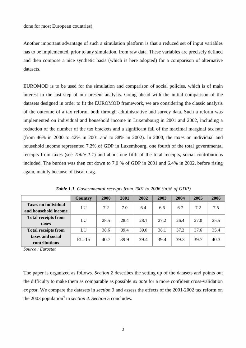
(from 46% in 2000 to 42% in 2001 and to 38% in 2002). In 2000, the taxes on individual and

household income represented 7.2% of GDP in Luxembourg, one fourth of the total governmental

receipts from taxes (see Table 1.1) and about one fifth of the total receipts, social contributions

included. The burden was then cut down to 7.0 % of GDP in 2001 and 6.4% in 2002, before rising

again, mainly because of fiscal drag.

Table 1.1 Governmental receipts from 2001 to 2006 (in % of GDP)

Country 2000 2001 2002 2003 2004 2005 2006 Taxes on individual

and household income LU 7.2 7.0 6.4 6.6 6.7 7.2 7.5

Total receipts from taxes

LU 28.5 28.4 28.1 27.2 26.4 27.0 25.5

Total receipts from taxes and social contributions

LU 38.6 39.4 39.0 38.1 37.2 37.6 35.4

EU-15 40.7 39.9 39.4 39.4 39.3 39.7 40.3

Source : Eurostat

The paper is organized as follows. Section 2 describes the setting up of the datasets and points out

the difficulty to make them as comparable as possible ex ante for a more confident cross-validation

ex post. We compare the datasets in section 3 and assess the effects of the 2001-2002 tax reform on

the 2003 population4 in section 4. Section 5 concludes.

4

2. SETTING UP THE DATASETS THROUGH THE EUROMOD INPUT FRAMEWORK

We introduce the main characteristics of the datasets, their initial setting-up in conformity with the

EUROMOD input framework, adaptations needed for making them as comparable as possible, and

finally the implications of some methodological choices.

2.1 Setting up initial data from the PSELL survey data

Luxembourg, as partner of the EUROMOD and MICRESA projects, is a user of the EUROMOD

model, up to now based on the Luxembourg household panel (PSELL5). For this exercise we use

the version 3/2004 covering income reference year 2003. The PSELL 3 data are used in

Luxembourg as a basis for the European Union Statistics on Income and Living Conditions6 (EU-

SILC). This is our first source of data. It is targeting the resident population of Luxembourg

(“international civil servants” included) through a sample of about 3,600 private households (nearly

9,800 persons). Institutional households (mainly elderly people residing in institutions) are not

covered by the survey. The unit of analysis is the “residence” household (living in the same house).

The sample configuration relies on (i) estimations of the resident population as of 1st of January

2004 by the Luxembourg Central Service for Statistics and Economic Studies7 (STATEC) and on

(ii) the most recent Luxembourg population census (15th of February 2001). The data collection

method is the face-to-face interview.

Information about all kinds of gross earnings are collected through the survey, including labor

income, investment and property income, social benefits in cash, private transfers, etc.

2.2 Setting up initial data from the Social Security Data Warehouse

Our second source of data for EUROMOD is the Social Security Data Warehouse recently built up

by the IGSS8 administration in Luxembourg for the year 2003. The main objective of the Data

Warehouse is to compose a normalized and exhaustive basis for the generation of statistics serving

diversified purposes (general reports, OECD, etc). The Data Warehouse is gathering all information

from several operational files of Social Security and other administrations (e.g. the National

Population Registry) which are of interest for social protection analysis : monthly and yearly

information on affiliation to social security, social contributions and benefits like pensions or family

allowances, etc. The basic unit is the individual. Administrative data, exhaustive in their universe of

definition, are neither related to a sampling process nor to high non response rates which require

5

weighting and imputation on the survey data side. Yet, these are not free of errors.

No information from the fiscal administration is made available for the building-up of the Data

Warehouse. However, labor earnings are partially known from the IGSS administration as they are

needed for the calculation of the social contributions paid either by the employer or the earner

himself when self-employed or socially insured on a voluntary basis. Consequently, three

limitations are to be noticed in the data. First, as in Luxembourg wages “declared” to the social

security are allowed to be truncated when greater than seven times the Minimum Social Wage9, it

may happen that labor earnings are truncated for high wages. Second, the earnings of the persons

who pay social contributions on a voluntary basis are most probably far departing from the real

state. Finally, farmers’ income cannot be properly determined either. On top of those limitations,

no information is available in the Data Warehouse for capital income and private transfers.

Taking the relationships that can be observed between the individuals in the Data Warehouse,

“Families” are constructed on a “fiscal basis”. “Residence” households, which are the unit of

analysis in PSELL, cannot be identified through available administrative data10. The households are

therefore built up in another way as follows. First, spouses11 are identified as a basis for the

household. This means that unmarried cohabitants do not appear as linked in the database (they

belong to different fiscal households), indeed in conformity with fiscal rules which are described in

the appendix. Second, a link is created between the children (basically, either unmarried and more

than 21 years old or older but still a student or disabled) and their parents through the family

benefits raised by the latter during the year12.

Only persons for whom positive earnings (either income or allowance) can be identified in the Data

Warehouse are included into the EUROMOD input database. The voluntary insured or coinsured

individuals are included as well. An implication is that “international civil servants” residing in

Luxembourg may not appear in the EUROMOD input database (they usually neither contribute to,

nor benefit from -in monetary terms-, the social security system in Luxembourg). Of course, in

conformity with the PSELL database, residents only are eligible13. A last remark concerns the

persons living in institutional households. Due to the fact that it is impossible to identify them in the

Data Warehouse, they are included in the EUROMOD input database built up from the Data

Warehouse, as opposed to the one built up from survey data.

6

2.3 Improving comparability of the EUROMOD input datasets

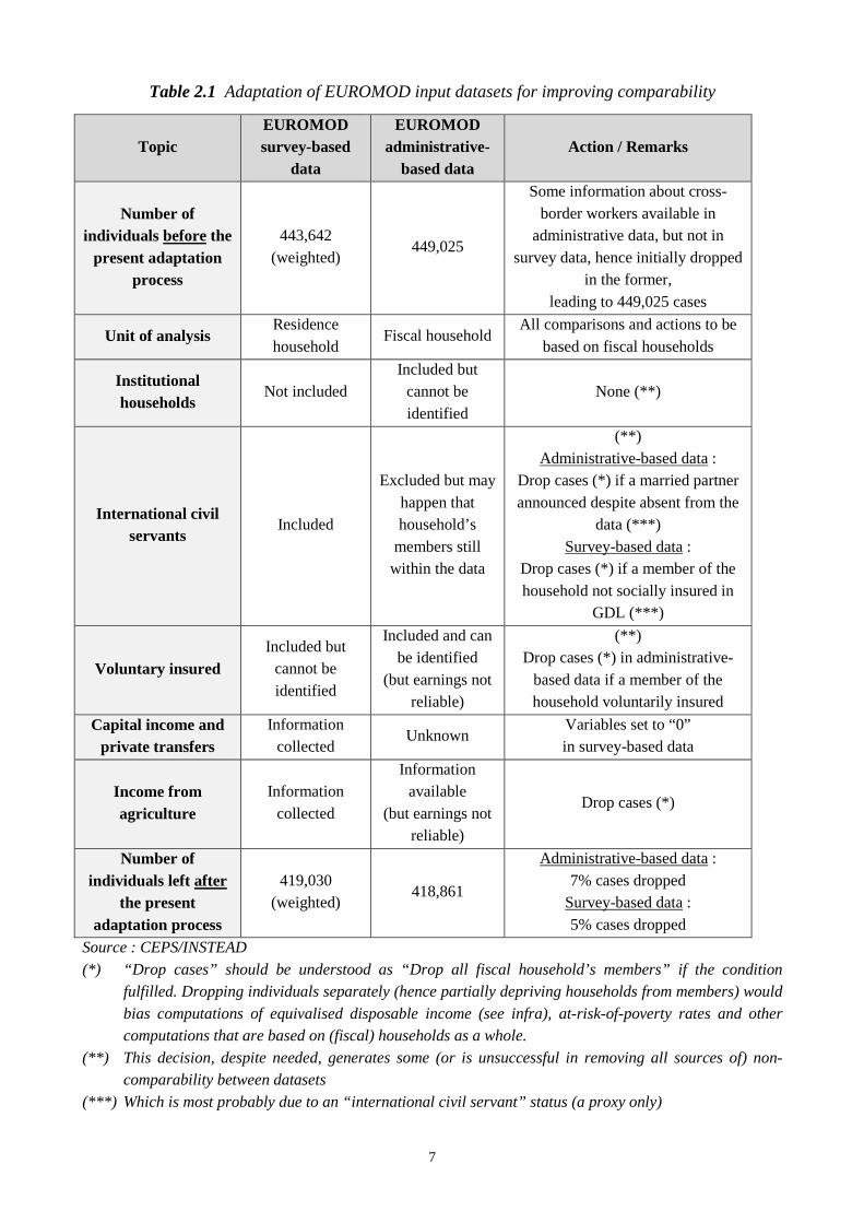
Given our main objective (see Introduction), it seems important to dispose of identifiable

dissimilarities between the initial datasets as regards their respective populations and the lack of

precision in some important (income-related) variables. Table 2.1 summarizes the question and

gives an insight about complementary adaptations which are needed for an ex ante better

comparability of the EUROMOD input datasets. We can see, for example, that capital income has

to be dropped from the survey-based data because no information is available about such an income

in the administrative-based data. Keeping capital income on one side only would bias our results

and weaken comparability of outcomes.

Individuals receiving an income from agriculture are dropped as well (both sides, for comparability

reasons) because methodological limits imply for the administrative-based dataset an imperfect link

only between the reality of earnings and the contents of the income variable on this side. In all

cases, when individuals are dropped, all members of the household follow in order to avoid bias due

to a change in the structure of the household, a bias that might be transferred downstream (see

infra).

While comparing monetary characteristics, the “equivalised disposable income” of households will

play a crucial role. As it is well known, the equivalised disposable income is the ratio of total

disposable income14 to the equivalent weight of the household. Following the so-called “OECD-

modified scale”, we assign a value (weight) of 1 to the household head, of 0.5 to each additional

adult member and of 0.3 to each child (less than 14 years old). The idea is to allow comparison (of

well-being) between families whose compositions differ while taking into account the economies of

scale a family of several persons is benefitting from compared to a single person. The equivalised

disposable income (which is called from now on “equivalised income” for short) is evaluated at the

household level. Each member of the household is then attributed this (common) value of

equivalised income.

Most usually in the literature, the “residence” household does matter, rather than the “fiscal” one.

Departing from this, we work with fiscal households, whatever survey-based or administrative-

based data. This induces two effects which may generate some discrepancies between our results

and the results based on (as they usually are) residence households.

7

Table 2.1 Adaptation of EUROMOD input datasets for improving comparability

Topic EUROMOD survey-based

data

EUROMOD administrative-

based data Action / Remarks

Number of individuals before the

present adaptation process

443,642 (weighted)

449,025

Some information about cross-border workers available in

administrative data, but not in survey data, hence initially dropped

in the former, leading to 449,025 cases

Unit of analysis Residence household

Fiscal household All comparisons and actions to be

based on fiscal households

Institutional households

Not included Included but

cannot be identified

None (**)

International civil servants

Included

Excluded but may happen that household’s

members still within the data

(**) Administrative-based data :

Drop cases (*) if a married partner announced despite absent from the

data (***) Survey-based data :

Drop cases (*) if a member of the household not socially insured in

GDL (***)

Voluntary insured Included but

cannot be identified

Included and can be identified

(but earnings not reliable)

(**) Drop cases (*) in administrative-

based data if a member of the household voluntarily insured

Capital income and private transfers

Information collected

Unknown Variables set to “0” in survey-based data

Income from agriculture

Information collected

Information available

(but earnings not reliable)

Drop cases (*)

Number of individuals left after

the present adaptation process

419,030 (weighted)

418,861

Administrative-based data : 7% cases dropped

Survey-based data : 5% cases dropped

Source : CEPS/INSTEAD

(*) “Drop cases” should be understood as “Drop all fiscal household’s members” if the condition fulfilled. Dropping individuals separately (hence partially depriving households from members) would

bias computations of equivalised disposable income (see infra), at-risk-of-poverty rates and other computations that are based on (fiscal) households as a whole.

(**) This decision, despite needed, generates some (or is unsuccessful in removing all sources of) non-comparability between datasets

(***) Which is most probably due to an “international civil servant” status (a proxy only)

8

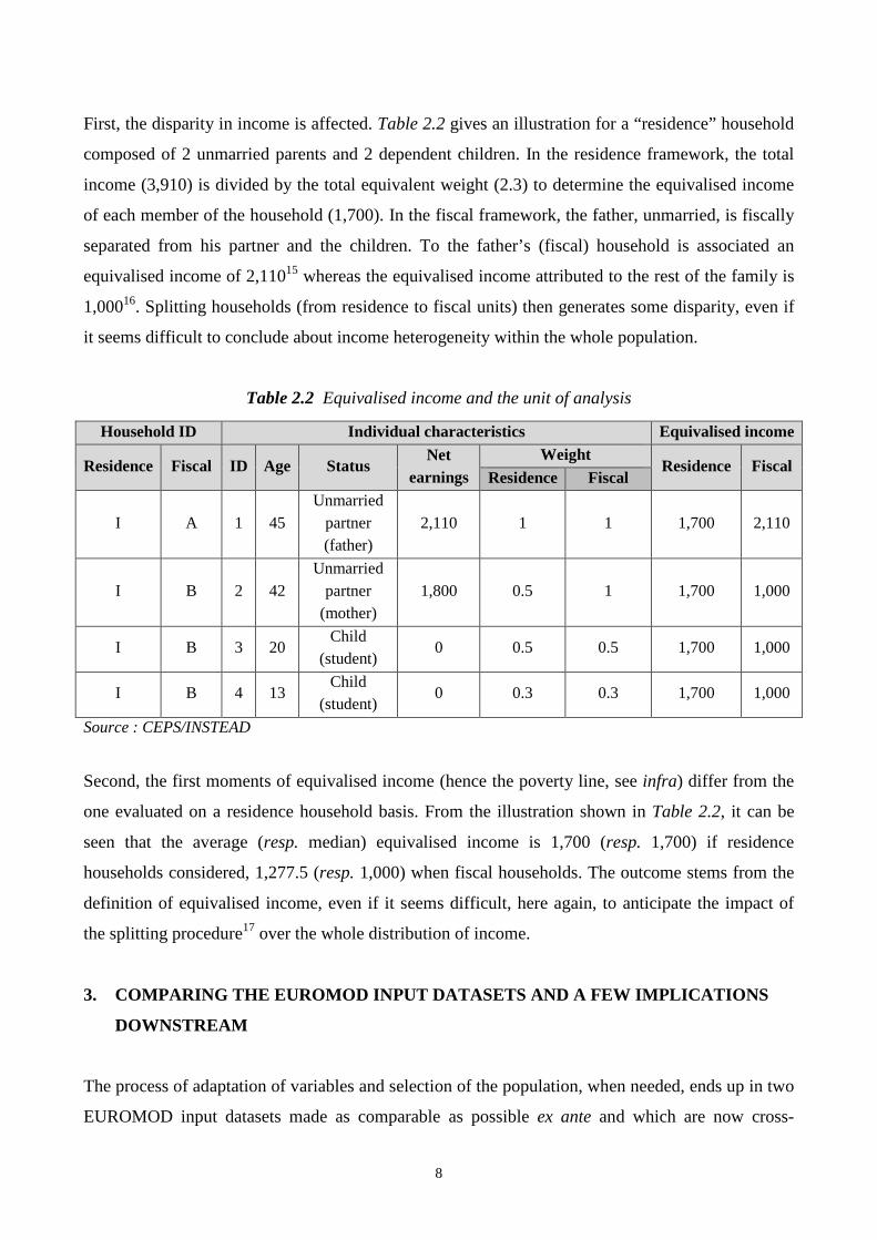
First, the disparity in income is affected. Table 2.2 gives an illustration for a “residence” household

composed of 2 unmarried parents and 2 dependent children. In the residence framework, the total

income (3,910) is divided by the total equivalent weight (2.3) to determine the equivalised income

of each member of the household (1,700). In the fiscal framework, the father, unmarried, is fiscally

separated from his partner and the children. To the father’s (fiscal) household is associated an

equivalised income of 2,11015 whereas the equivalised income attributed to the rest of the family is

1,00016. Splitting households (from residence to fiscal units) then generates some disparity, even if

it seems difficult to conclude about income heterogeneity within the whole population.

Table 2.2 Equivalised income and the unit of analysis

Household ID Individual characteristics Equivalised income

Residence Fiscal ID Age Status Net

earnings Weight

Residence Fiscal Residence Fiscal

I A 1 45 Unmarried

partner (father)

2,110 1 1 1,700 2,110

I B 2 42 Unmarried

partner (mother)

1,800 0.5 1 1,700 1,000

I B 3 20 Child

(student) 0 0.5 0.5 1,700 1,000

I B 4 13 Child

(student) 0 0.3 0.3 1,700 1,000


Second, the first moments of equivalised income (hence the poverty line, see infra) differ from the

one evaluated on a residence household basis. From the illustration shown in Table 2.2, it can be

seen that the average (resp. median) equivalised income is 1,700 (resp. 1,700) if residence

households considered, 1,277.5 (resp. 1,000) when fiscal households. The outcome stems from the

definition of equivalised income, even if it seems difficult, here again, to anticipate the impact of

the splitting procedure17 over the whole distribution of income.

3. COMPARING THE EUROMOD INPUT DATASETS AND A FEW IMP LICATIONS

DOWNSTREAM

The process of adaptation of variables and selection of the population, when needed, ends up in two

EUROMOD input datasets made as comparable as possible ex ante and which are now cross-

9

validated at the household and individual levels.

3.1 The household level

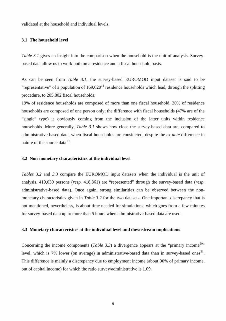
Table 3.1 gives an insight into the comparison when the household is the unit of analysis. Survey-

based data allow us to work both on a residence and a fiscal household basis.

As can be seen from Table 3.1, the survey-based EUROMOD input dataset is said to be

“representative” of a population of 169,62018 residence households which lead, through the splitting

procedure, to 205,802 fiscal households.

19% of residence households are composed of more than one fiscal household. 30% of residence

households are composed of one person only; the difference with fiscal households (47% are of the

“single” type) is obviously coming from the inclusion of the latter units within residence

households. More generally, Table 3.1 shows how close the survey-based data are, compared to

administrative-based data, when fiscal households are considered, despite the ex ante difference in

nature of the source data19.

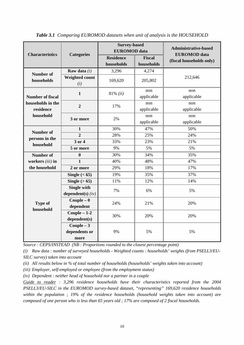
3.2 Non-monetary characteristics at the individual level

Tables 3.2 and 3.3 compare the EUROMOD input datasets when the individual is the unit of

analysis. 419,030 persons (resp. 418,861) are “represented” through the survey-based data (resp.

administrative-based data). Once again, strong similarities can be observed between the non-

monetary characteristics given in Table 3.2 for the two datasets. One important discrepancy that is

not mentioned, nevertheless, is about time needed for simulations, which goes from a few minutes

for survey-based data up to more than 5 hours when administrative-based data are used.

3.3 Monetary characteristics at the individual level and downstream implications

Concerning the income components (Table 3.3) a divergence appears at the “primary income20”

level, which is 7% lower (on average) in administrative-based data than in survey-based ones21.

This difference is mainly a discrepancy due to employment income (about 90% of primary income,

out of capital income) for which the ratio survey/administrative is 1.09.

10

Table 3.1 Comparing EUROMOD datasets when unit of analysis is the HOUSEHOLD

Characteristics Categories

Survey-based EUROMOD data

Administrative-based EUROMOD data

(fiscal households only) Residence households

Fiscal households

Number of households

Raw data (i) 3,296 4,274

212,646 Weighted count (i)

169,620 205,802

Number of fiscal households in the

residence household

1 81% (ii) non

applicable non

applicable

2 17% non

applicable non

applicable

3 or more 2% non

applicable non

applicable

Number of persons in the

household

1 30% 47% 50%

2 28% 25% 24%

3 or 4 33% 23% 21%

5 or more 9% 5% 5%

Number of workers (iii) in the household

0 30% 34% 35%

1 40% 48% 47%

2 or more 29% 18% 17%

Type of household

Single (< 65) 19% 35% 37%

Single (> 65) 11% 12% 14%

Single with dependent(s) (iv)

7% 6% 5%

Couple – 0 dependent

24% 21% 20%

Couple – 1-2 dependent(s)

30% 20% 20%

Couple – 3 dependents or

more 9% 5% 5%

Source : CEPS/INSTEAD (NB : Proportions rounded to the closest percentage point) (i) Raw data : number of surveyed households - Weighted counts : households’ weights (from PSELL3/EU-

SILC survey) taken into account (ii) All results below in % of total number of households (households’ weights taken into account)

(iii) Employer, self-employed or employee (from the employment status) (iv) Dependent : neither head of household nor a partner in a couple

Guide to reader : 3,296 residence households have their characteristics reported from the 2004 PSELL3/EU-SILC in the EUROMOD survey-based dataset, “representing” 169,620 residence households

within the population ; 19% of the residence households (household weights taken into account) are composed of one person who is less than 65 years old ; 17% are composed of 2 fiscal households.

11

Table 3.2 Comparing EUROMOD datasets when the unit of analysis is the INDIVIDUAL :

Non-monetary characteristics

Characteristics Categories Survey-based

EUROMOD data Administrative-based

EUROMOD data

Number of persons

Raw data (i) 8,657

418,861 Weighted count (i)

419,030

Gender Female 50.7% 50.5%

Male 49.3% 49.5%

Age Age < 18 22% 22%

18<= Age < 59 59% 59%

Age >= 60 19% 20%

Type of household

Single (< 65) 17% 19%

Single (> 65) 6% 7%

Single with dependent(s) (ii)

7% 6%


21% 21%

Couple – 1-2 dependent(s)

35% 35%

Couple – 3 dependents or

more 14% 12%

Number of workers (iii) in the household

0 25% 26%

1 45% 45%

2 or more 30% 29%

Source : CEPS/INSTEAD (NB : Proportions rounded to the closest percentage point) (i) Raw data : number of surveyed individuals - Weighted counts : individual weights (from PSELL3/EU-

SILC survey) taken into account (ii) Dependent : neither head of household nor a partner in a couple (iii) Employer, self-employed or employee (from the employment status)

The confidence interval shown in Table 3.3 for the primary income implies that the divergence

cannot be statistically imputed, for a confidence level of 95%22, to the sampling process on the

survey-side. Actually, the setting up of the data can help a little in understanding differences. Table

2.1 is mentioning, despite the adaptation process of the EUROMOD input datasets for improving

their comparability, some lack of similarity regarding the institutional households. Moreover,

individuals deceased or disappearing from the data records during the last year cannot be treated

perfectly the same way in both datasets. Taking roughly into account those dissimilarities23, it can

be shown that the difference in primary income might be reduced and the results made statistically

compatible given the sampling process24. It is also worth mentioning some discrepancy regarding

12

income measurement. For example, survey-based data include in “employment” earnings sickness

replacement wages when relating to very short periods.

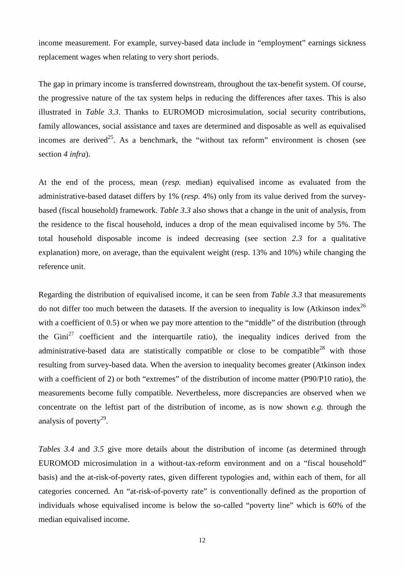
The gap in primary income is transferred downstream, throughout the tax-benefit system. Of course,

the progressive nature of the tax system helps in reducing the differences after taxes. This is also

illustrated in Table 3.3. Thanks to EUROMOD microsimulation, social security contributions,

family allowances, social assistance and taxes are determined and disposable as well as equivalised

incomes are derived25. As a benchmark, the “without tax reform” environment is chosen (see

section 4 infra).

At the end of the process, mean (resp. median) equivalised income as evaluated from the

administrative-based dataset differs by 1% (resp. 4%) only from its value derived from the survey-

based (fiscal household) framework. Table 3.3 also shows that a change in the unit of analysis, from

the residence to the fiscal household, induces a drop of the mean equivalised income by 5%. The

total household disposable income is indeed decreasing (see section 2.3 for a qualitative

explanation) more, on average, than the equivalent weight (resp. 13% and 10%) while changing the

reference unit.

Regarding the distribution of equivalised income, it can be seen from Table 3.3 that measurements

do not differ too much between the datasets. If the aversion to inequality is low (Atkinson index26

with a coefficient of 0.5) or when we pay more attention to the “middle” of the distribution (through

the Gini27 coefficient and the interquartile ratio), the inequality indices derived from the

administrative-based data are statistically compatible or close to be compatible28 with those

resulting from survey-based data. When the aversion to inequality becomes greater (Atkinson index

with a coefficient of 2) or both “extremes” of the distribution of income matter (P90/P10 ratio), the

measurements become fully compatible. Nevertheless, more discrepancies are observed when we

concentrate on the leftist part of the distribution of income, as is now shown e.g. through the

analysis of poverty29.

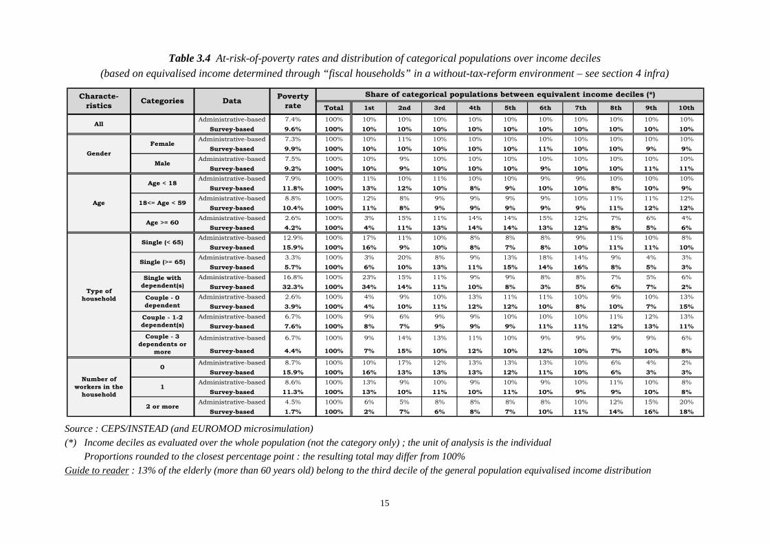
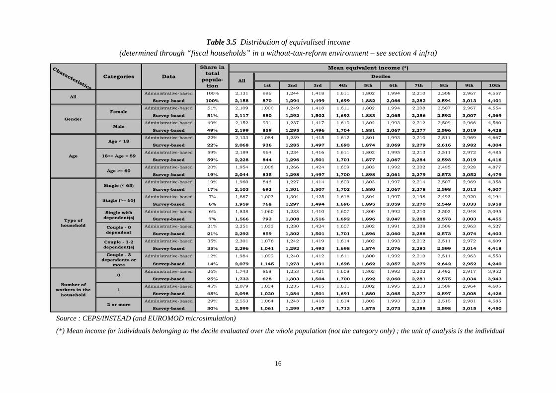
Tables 3.4 and 3.5 give more details about the distribution of income (as determined through

EUROMOD microsimulation in a without-tax-reform environment and on a “fiscal household”

basis) and the at-risk-of-poverty rates, given different typologies and, within each of them, for all

categories concerned. An “at-risk-of-poverty rate” is conventionally defined as the proportion of

individuals whose equivalised income is below the so-called “poverty line” which is 60% of the

median equivalised income.

13

Table 3.3 Comparing EUROMOD datasets when the unit of analysis is the INDIVIDUAL :

Monetary characteristics and implications downstream (*),

in EUR / month (except Equivalent weight and Inequality coefficients)

Characteristics Categories

Survey-based EUROMOD data Administrative-

based EUROMOD data Residence

households Fiscal households

Primary income (i), out of capital income (ii)

(on average)

1,493 [1,416 – 1,570] (iii)

1,384

Capital income (ii) (on average)

78 Not available in

source data Standard disposable income

(iv), (vi) (on average)

1,529 1,518

Total household disposable income (v), (vi)

(on average) 4,395 3,811 3,720

OECD equivalent weight (on average) 1.97 1.77 1.74

OECD equivalised

income (vi)

Mean 2,276 2,158 2,131 Median 2,076 1,980 1,898

Poverty line (60% of the median) 1,246

1,188 [1,171 – 1,205]

(iii) 1,138

Gini coefficient Not computed 0.243

[0.236 – 0.249] (iii)

0.248

P75 / P25 ratio Not computed 1.727

[1.697 – 1.757] (iii)

1.760

Atkinson index (inequality aversion coefficient : 0.5) Not computed

0.048 [0.045 – 0.050]

(iii) 0.051

P90 / P10 ratio Not computed 2.798

[2.728 – 2.868] (iii)

2.809

Atkinson index (inequality aversion coefficient : 2.0) Not computed

0.227 [0.203 – 0.252]

(iii) 0.223

Source : CEPS/INSTEAD (and EUROMOD microsimulation)

(*) All amounts before/without the 2001-2002 tax reform in Luxembourg (see section 4 infra) (i) Primary income (see footnote 20) = Gross earnings all sources (out of public pensions), before

Employee social contributions and Income taxation, and out of Social benefits (ii) Capital income = Gross property income + Gross investment income

(iii) All 95 % STATA “bootstrap” confidence intervals (500 replications) (iv) Standard disposable income = Primary income – Employee social contributions

– Income taxes + Social benefits in cash (Reminder : the capital income is here excluded from computations)

(v) Total disposable income within the household, attributed to each member in conformity with the computation of the equivalised income

(vi) Evaluated through EUROMOD microsimulation

14

It is worth noticing that the usual basis for analysis of poverty is the residence household and not

the fiscal one, which makes a difference regarding the household disposable income, the

equivalised income of the members hence the poverty line and the at-risk-of poverty rates (see

Table 3.3). Nevertheless, we are here mentioning indicators regarding the fiscal households. Indeed,

we are constrained by the administrative-based data where no information is available about

residence households. Fortunately, we can also remind our main objective which is the comparison

of the datasets for cross-validation rather than a specific standard poverty analysis.

The at-risk-of-poverty rates are higher, on average30 as well as for most categories31, when

evaluated through the survey-based data32 (Table 3.4). It can also be shown that, regarding the

whole population, the intensity of poverty, measured by the “income gap ratio”33, is higher through

survey-based data. More generally, usual findings follow : younger people, singles either less-than-

65-years-old or with dependent(s)34 and the members of households where nobody is working are

more at risk of poverty than the other categories within the population, whatever the dataset under

consideration. It can be seen that those populations are more concentrated in the first deciles of

income distributions than others. Singles with dependent(s) and the households with no worker also

experience less equivalised income, on average, than the members of the respective associated

categories (Table 3.5). Nevertheless, no systematic link can be observed between the mean level of

income within a category and its at-risk-of-poverty rate.

A few striking discrepancies are to be noticed between the datasets, for example concerning the

“singles with dependent(s)” who are marked twice more at risk of poverty in survey-based data. But

we should be cautious about interpretation, given the sampling nature of the survey which might

induce bias as far as a sub-group (7% of the population, see Table 3.5) only is concerned. The gap

in poverty between men and women is also shown close to 0% under administrative-based data but

not far from 1% when survey-based data are considered.

It must be noticed again that, due to the fact that the calculation have been made on the “fiscal

households” and not on “residence households”, it makes no sense to compare these figures with

poverty rates published at the European and the national levels.

15

Table 3.4 At-risk-of-poverty rates and distribution of categorical populations over income deciles

(based on equivalised income determined through “fiscal households” in a without-tax-reform environment – see section 4 infra)


(*) Income deciles as evaluated over the whole population (not the category only) ; the unit of analysis is the individual Proportions rounded to the closest percentage point : the resulting total may differ from 100%

Guide to reader : 13% of the elderly (more than 60 years old) belong to the third decile of the general population equivalised income distribution

Total 1st 2nd 3rd 4th 5th 6th 7th 8th 9th 10th

Administrative-based 7.4% 100% 10% 10% 10% 10% 10% 10% 10% 10% 10% 10%

Survey-based 9.6% 100% 10% 10% 10% 10% 10% 10% 10% 10% 10% 10%


Survey-based 9.9% 100% 10% 10% 10% 10% 10% 11% 10% 10% 9% 9%


Survey-based 9.2% 100% 10% 9% 10% 10% 10% 9% 10% 10% 11% 11%


Survey-based 11.8% 100% 13% 12% 10% 8% 9% 10% 10% 8% 10% 9%


Survey-based 10.4% 100% 11% 8% 9% 9% 9% 9% 9% 11% 12% 12%


Survey-based 4.2% 100% 4% 11% 13% 14% 14% 13% 12% 8% 5% 6%


Survey-based 15.9% 100% 16% 9% 10% 8% 7% 8% 10% 11% 11% 10%


Survey-based 5.7% 100% 6% 10% 13% 11% 15% 14% 16% 8% 5% 3%


Survey-based 32.3% 100% 34% 14% 11% 10% 8% 3% 5% 6% 7% 2%


Survey-based 3.9% 100% 4% 10% 11% 12% 12% 10% 8% 10% 7% 15%


Survey-based 7.6% 100% 8% 7% 9% 9% 9% 11% 11% 12% 13% 11%


Survey-based 4.4% 100% 7% 15% 10% 12% 10% 12% 10% 7% 10% 8%


Survey-based 15.9% 100% 16% 13% 13% 13% 12% 11% 10% 6% 3% 3%


Survey-based 11.3% 100% 13% 10% 11% 10% 11% 10% 9% 9% 10% 8%


Survey-based 1.7% 100% 2% 7% 6% 8% 7% 10% 11% 14% 16% 18%

Number of

workers in the

household

0

1

2 or more

Share of categorical populations between equivalent income deciles (*)

All

Age

Age < 18

18<= Age < 59

Age >= 60

Type of

household

Single (< 65)

Single (>= 65)

Single with

dependent(s)

Couple - 0

dependent

Couple - 1-2

dependent(s)

Couple - 3

dependents or

more

Gender

Female

Male

DataPoverty

rate

Characte-

risticsCategories

16

Table 3.5 Distribution of equivalised income (determined through “fiscal households” in a without-tax-reform environment – see section 4 infra)


(*) Mean income for individuals belonging to the decile evaluated over the whole population (not the category only) ; the unit of analysis is the individual

1st 2nd 3rd 4th 5th 6th 7th 8th 9th 10th

Administrative-based 100% 2,131 996 1,244 1,418 1,611 1,802 1,994 2,210 2,508 2,967 4,557

Survey-based 100% 2,158 870 1,294 1,499 1,699 1,882 2,066 2,282 2,594 3,013 4,401

Administrative-based 51% 2,109 1,000 1,249 1,418 1,611 1,802 1,994 2,208 2,507 2,967 4,554

Survey-based 51% 2,117 880 1,292 1,502 1,693 1,883 2,065 2,286 2,592 3,007 4,369


Survey-based 49% 2,199 859 1,295 1,496 1,704 1,881 2,067 2,277 2,596 3,019 4,428


Survey-based 22% 2,068 936 1,285 1,497 1,693 1,874 2,069 2,279 2,616 2,982 4,304


Survey-based 59% 2,228 844 1,296 1,501 1,701 1,877 2,067 2,284 2,593 3,019 4,416


Survey-based 19% 2,044 835 1,298 1,497 1,700 1,898 2,061 2,279 2,573 3,052 4,479


Survey-based 17% 2,103 692 1,301 1,507 1,702 1,880 2,067 2,278 2,598 3,013 4,507


Survey-based 6% 1,959 768 1,297 1,494 1,696 1,895 2,059 2,270 2,549 3,033 3,958


Survey-based 7% 1,566 792 1,308 1,516 1,692 1,896 2,047 2,288 2,573 3,003 4,455


Survey-based 21% 2,292 859 1,302 1,501 1,701 1,896 2,060 2,288 2,573 3,074 4,403


Survey-based 35% 2,296 1,041 1,292 1,493 1,698 1,874 2,076 2,283 2,599 3,014 4,418


Survey-based 14% 2,079 1,145 1,273 1,491 1,698 1,862 2,057 2,279 2,642 2,952 4,240


Survey-based 25% 1,733 628 1,303 1,504 1,700 1,892 2,060 2,281 2,575 3,034 3,943


Survey-based 45% 2,098 1,020 1,284 1,501 1,691 1,880 2,065 2,277 2,597 3,008 4,426


Survey-based 30% 2,599 1,061 1,299 1,487 1,713 1,875 2,073 2,288 2,598 3,015 4,450

Number of

workers in the

household

0

1

2 or more

Single (< 65)

Single (>= 65)

Single with

dependent(s)

Couple - 0

dependent

Mean equivalent income (*)

DecilesAll

Share in

total

popula-

tion

Categories

Characteristics

Data

All

Couple - 3

dependents or

more

Female

Male

Age < 18

18<= Age < 59

Age >= 60

Couple - 1-2

dependent(s)

Gender

Type of

household

Age

17

4. A COMPARATIVE APPLICATION TO THE ANALYSIS OF A TAX REFORM

In the previous sections, we have emphasized similarities and discrepancies observed between the

survey-based and administrative-based datasets seen as raw data, even if redesigned in order to fit

the EUROMOD input framework. We are now going a step further and considering the implication

of an alternative use of the datasets for the classic analysis of a tax reform.

Such a reform was implemented on individual and household income in Luxembourg in 2001 and

2002. The characteristics of the reform are described in the appendix and we are here highlighting

its main (rather common) outlines only :

- The first tax bracket is enlarged, which means that the minimum income before tax is

increased, from 6,693 EUR in 2000 up to 9,750 EUR in 2002

- The number of tax brackets is reduced, from 18 down to 17 in 2002 and band widths are made

uniform to 1,650 EUR in 2002

- The maximum tax rate significantly decreases, from 46% to 38% in 2002

This section analyses the distributional effects of the reform on the 2003 population. All results are

derived from both the administrative-based and survey-based datasets. We first develop the

methodological framework chosen for the analysis in order to make the comparison as accurate as

possible. Then, we present an overall view on inequalities, with and without the tax reform, and on

changes in disposable income by category of population. Finally, we concentrate more on the left-

hand side of the distribution through looking into the proportion and characteristics of non-tax

payers and finally examining the at-risk-of-poverty rates.

4.1 Methodological framework for analysis

Given the 2001-2002 fiscal changes in Luxembourg, the initial idea is to compare the 2000 situation

with the 2002 one, whatever the way for proceeding. Nevertheless, the changes over a 2-year period

regarding the economy and the social field reflect several influences, not limited to the evolution of

fiscal rules. During this period, the population (age, composition of households, etc) changes, the

economy faces some inflation and hopefully economic growth (hence an impact on real earnings),

the distribution of primary income may be altered, policies other than the fiscal one can be

amended, unemployment may not be stable, etc (Fuchs and Lietz, 2007, Immervoll et al., 2006). All

these first-round effects can still be completed either through behavioral answers of the population

18

(e.g. labor supply), or through feedback effects from the economy as a whole (e.g. prices), or

through sectorial budgetary constraints (e.g. individual or public accounts).

We would like to strictly avoid the changes not directly resulting from the tax reform in itself.

Moreover, our main objective remains the comparison of specific datasets. These are the reasons

why we choose to concentrate on a given year, as far as the economy and the social field are

concerned, with a simple treatment of the tax-benefit environment. In the benchmark35, the tax

system is designed as before the 2001-2002 reform, conforming to the brief description made earlier

(and completed in the appendix). The alternative is then simply to set up the tax system as on 2002,

that means in its post-reform state. On the benefit side, no change is to be mentioned between the

benchmark and the alternative. The year 2003 (rather than 2002) is chosen as a basis for analysis.

This is simply due to a constraint on administrative data the first set of which was made available

for the year 2003 only.

Altogether, these options lead to the following story. We compare two situations, one where the

Luxembourg population in 2003 faces the real tax-benefit system of 2003, the other one where the

tax system of 2000 is applied to the same population, everything else (e.g. benefits) untouched. In

other words, we ask what had happened for the population in 2003, had the 2000 tax system either

been frozen, on one side, or be replaced by the new 2003 tax system, on the other side. The

hypothesis of an invariant tax system through time makes sense in Luxembourg where the tax rules

are basically not changing between reforms (e.g. no adaptation relating to the consumption price

index is made on an automatic basis), what was observed e.g. from 2002 up to the beginning of

2008. The benefit side, on the contrary, is following in Luxembourg a more dynamic track, which

makes quite natural our hypothesis of a benefit system designed in 2003 as it really was, whatever

the tax system.

Given our framework for analysis, we assess the distributional effects of the tax reform on

individual income through the tax-benefit static microsimulation model EUROMOD. EUROMOD

is a flexible tool that enables research on the first-round effects36 of policy reforms that have an

impact on earnings (mainly through social contributions, taxes and cash benefits), hence on poverty

and inequality (Sutherland, 2001). Microsimulation models rely on micro-data representative of a

population (households and individuals) and designed so that we can hold most influences constant

(e.g. the benefit system, including non-take-up behavior, and demographic characteristics) and

focus on the effect of one change at a time (e.g. the tax system and/or the dataset).

19

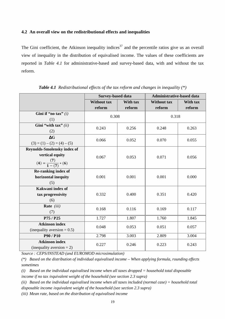
4.2 An overall view on the redistributional effects and inequalities

The Gini coefficient, the Atkinson inequality indices37 and the percentile ratios give us an overall

view of inequality in the distribution of equivalised income. The values of these coefficients are

reported in Table 4.1 for administrative-based and survey-based data, with and without the tax

reform.

Table 4.1 Redistributional effects of the tax reform and changes in inequality (*)

Survey-based data Administrative-based data

Without tax reform

With tax reform

Without tax reform

With tax reform

Gini if “no tax” (i) (1)

0.308 0.318

Gini “with tax” (ii) (2)

0.243 0.256 0.248 0.263

∆∆∆∆G (3) = (1) – (2) = (4) – (5)

0.066 0.052 0.070 0.055

Reynolds-Smolensky index of vertical equity

��

0.067 0.053 0.071 0.056

Re-ranking index of horizontal inequity

(5) 0.001 0.001 0.001 0.000

Kakwani index of tax progressivity

(6) 0.332 0.400 0.351 0.420

Rate (iii) (7)

0.168 0.116 0.169 0.117

P75 / P25 1.727 1.807 1.760 1.845

Atkinson index (inequality aversion = 0.5)

0.048 0.053 0.051 0.057

P90 / P10 2.798 3.003 2.809 3.004

Atkinson index (inequality aversion = 2)

0.227 0.246 0.223 0.243

Source : CEPS/INSTEAD (and EUROMOD microsimulation) (*) Based on the distribution of individual equivalised income – When applying formula, rounding effects

sometimes (i) Based on the individual equivalised income when all taxes dropped = household total disposable

income if no tax /equivalent weight of the household (see section 2.3 supra) (ii) Based on the individual equivalised income when all taxes included (normal case) = household total

disposable income /equivalent weight of the household (see section 2.3 supra) (iii) Mean rate, based on the distribution of equivalised income

20

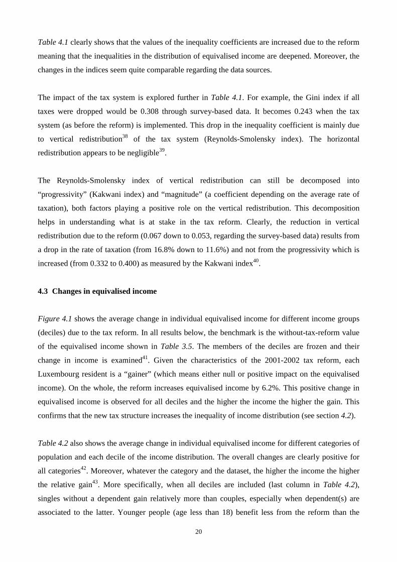
Table 4.1 clearly shows that the values of the inequality coefficients are increased due to the reform

meaning that the inequalities in the distribution of equivalised income are deepened. Moreover, the

changes in the indices seem quite comparable regarding the data sources.

The impact of the tax system is explored further in Table 4.1. For example, the Gini index if all

taxes were dropped would be 0.308 through survey-based data. It becomes 0.243 when the tax

system (as before the reform) is implemented. This drop in the inequality coefficient is mainly due

to vertical redistribution38 of the tax system (Reynolds-Smolensky index). The horizontal

redistribution appears to be negligible39.

The Reynolds-Smolensky index of vertical redistribution can still be decomposed into

“progressivity” (Kakwani index) and “magnitude” (a coefficient depending on the average rate of

taxation), both factors playing a positive role on the vertical redistribution. This decomposition

helps in understanding what is at stake in the tax reform. Clearly, the reduction in vertical

redistribution due to the reform (0.067 down to 0.053, regarding the survey-based data) results from

a drop in the rate of taxation (from 16.8% down to 11.6%) and not from the progressivity which is

increased (from 0.332 to 0.400) as measured by the Kakwani index40.

4.3 Changes in equivalised income

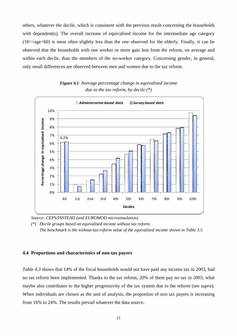
Figure 4.1 shows the average change in individual equivalised income for different income groups

(deciles) due to the tax reform. In all results below, the benchmark is the without-tax-reform value

of the equivalised income shown in Table 3.5. The members of the deciles are frozen and their

change in income is examined41. Given the characteristics of the 2001-2002 tax reform, each

Luxembourg resident is a “gainer” (which means either null or positive impact on the equivalised

income). On the whole, the reform increases equivalised income by 6.2%. This positive change in

equivalised income is observed for all deciles and the higher the income the higher the gain. This

confirms that the new tax structure increases the inequality of income distribution (see section 4.2).

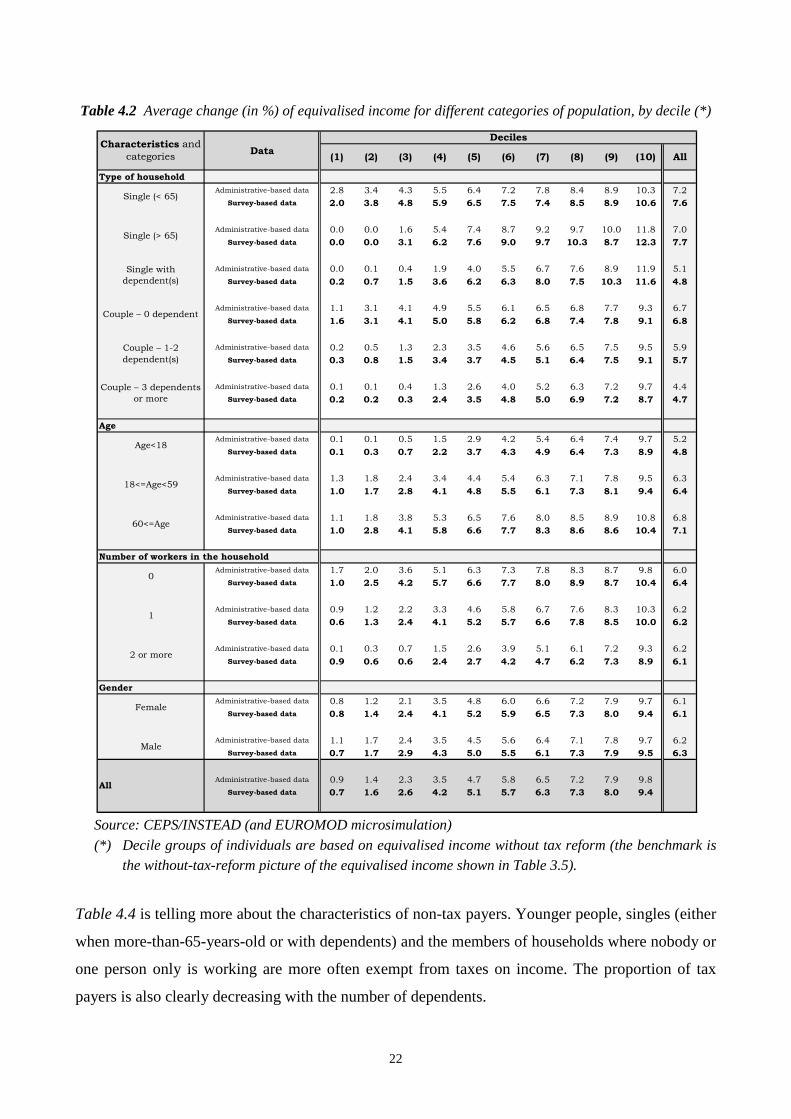
Table 4.2 also shows the average change in individual equivalised income for different categories of

population and each decile of the income distribution. The overall changes are clearly positive for

all categories42. Moreover, whatever the category and the dataset, the higher the income the higher

the relative gain43. More specifically, when all deciles are included (last column in Table 4.2),

singles without a dependent gain relatively more than couples, especially when dependent(s) are

associated to the latter. Younger people (age less than 18) benefit less from the reform than the

21

others, whatever the decile, which is consistent with the previous result concerning the households

with dependent(s). The overall increase of equivalised income for the intermediate age category

(18<=age<60) is most often slightly less than the one observed for the elderly. Finally, it can be

observed that the households with one worker or more gain less from the reform, on average and

within each decile, than the members of the no-worker category. Concerning gender, in general,

only small differences are observed between men and women due to the tax reform.

Figure 4.1 Average percentage change in equivalised income

due to the tax reform, by decile (*)

Source: CEPS/INSTEAD (and EUROMOD microsimulation) (*) Decile groups based on equivalised income without tax reform.

The benchmark is the without-tax-reform value of the equivalised income shown in Table 3.5

4.4 Proportions and characteristics of non-tax payers

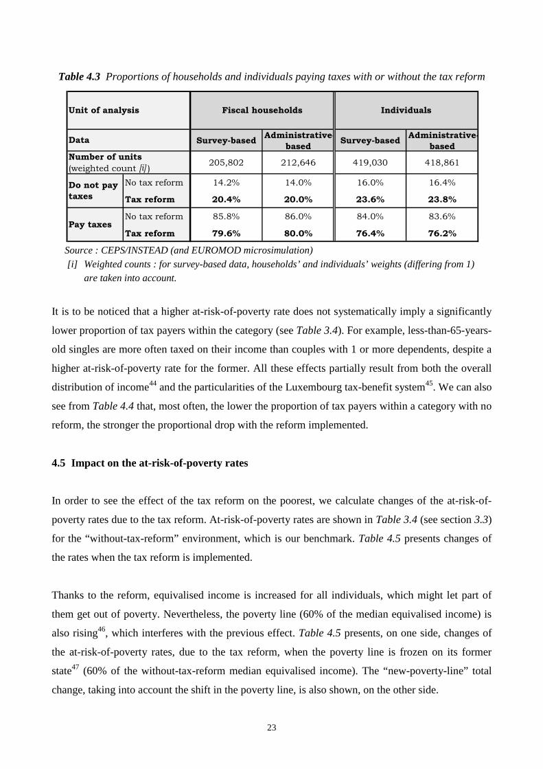
Table 4.3 shows that 14% of the fiscal households would not have paid any income tax in 2003, had

no tax reform been implemented. Thanks to the tax reform, 20% of them pay no tax in 2003, what

maybe also contributes to the higher progressivity of the tax system due to the reform (see supra).

When individuals are chosen as the unit of analysis, the proportion of non tax payers is increasing

from 16% to 24%. The results prevail whatever the data source.

6.2%

0%

1%

2%

3%

4%

5%

6%

7%

8%

9%

10%

All 1st 2nd 3rd 4th 5th 6th 7th 8th 9th 10th

Pe

rce

nta

ge

ch

an

ge

in

eq

uiv

ali

sed

in

com

e

Deciles

Administrative-based data Survey-based data

22

Table 4.2 Average change (in %) of equivalised income for different categories of population, by decile (*)

Source: CEPS/INSTEAD (and EUROMOD microsimulation)

(*) Decile groups of individuals are based on equivalised income without tax reform (the benchmark is the without-tax-reform picture of the equivalised income shown in Table 3.5).

Table 4.4 is telling more about the characteristics of non-tax payers. Younger people, singles (either

when more-than-65-years-old or with dependents) and the members of households where nobody or

one person only is working are more often exempt from taxes on income. The proportion of tax

payers is also clearly decreasing with the number of dependents.

Data

Type of household

Administrative-based data 2.8 3.4 4.3 5.5 6.4 7.2 7.8 8.4 8.9 10.3 7.2

Survey-based data 2.0 3.8 4.8 5.9 6.5 7.5 7.4 8.5 8.9 10.6 7.6











Age







Number of workers in the household







Gender





Administrative-based data 0.9 1.4 2.3 3.5 4.7 5.8 6.5 7.2 7.9 9.8

Survey-based data 0.7 1.6 2.6 4.2 5.1 5.7 6.3 7.3 8.0 9.4

1

2 or more

Female

Male

All

Characteristics and

categories

Couple – 1-2

dependent(s)

Couple – 3 dependents

or more

Age<18

18<=Age<59

60<=Age

0

(10) All

Single (< 65)

Single (> 65)

Single with

dependent(s)


Deciles

(1) (2) (3) (4) (5) (6) (7) (8) (9)

23

Table 4.3 Proportions of households and individuals paying taxes with or without the tax reform


[i] Weighted counts : for survey-based data, households’ and individuals’ weights (differing from 1) are taken into account.

It is to be noticed that a higher at-risk-of-poverty rate does not systematically imply a significantly

lower proportion of tax payers within the category (see Table 3.4). For example, less-than-65-years-

old singles are more often taxed on their income than couples with 1 or more dependents, despite a

higher at-risk-of-poverty rate for the former. All these effects partially result from both the overall

distribution of income44 and the particularities of the Luxembourg tax-benefit system45. We can also

see from Table 4.4 that, most often, the lower the proportion of tax payers within a category with no

reform, the stronger the proportional drop with the reform implemented.

4.5 Impact on the at-risk-of-poverty rates

In order to see the effect of the tax reform on the poorest, we calculate changes of the at-risk-of-

poverty rates due to the tax reform. At-risk-of-poverty rates are shown in Table 3.4 (see section 3.3)

for the “without-tax-reform” environment, which is our benchmark. Table 4.5 presents changes of

the rates when the tax reform is implemented.

Thanks to the reform, equivalised income is increased for all individuals, which might let part of

them get out of poverty. Nevertheless, the poverty line (60% of the median equivalised income) is

also rising46, which interferes with the previous effect. Table 4.5 presents, on one side, changes of

the at-risk-of-poverty rates, due to the tax reform, when the poverty line is frozen on its former

state47 (60% of the without-tax-reform median equivalised income). The “new-poverty-line” total

change, taking into account the shift in the poverty line, is also shown, on the other side.

Survey-basedAdministrative-

basedSurvey-based

Administrative-

based

205,802 212,646 419,030 418,861

No tax reform 14.2% 14.0% 16.0% 16.4%

Tax reform 20.4% 20.0% 23.6% 23.8%

No tax reform 85.8% 86.0% 84.0% 83.6%

Tax reform 79.6% 80.0% 76.4% 76.2%

Fiscal households IndividualsUnit of analysis

Data

Pay taxes

Number of units

(weighted count [i] )

Do not pay

taxes

24

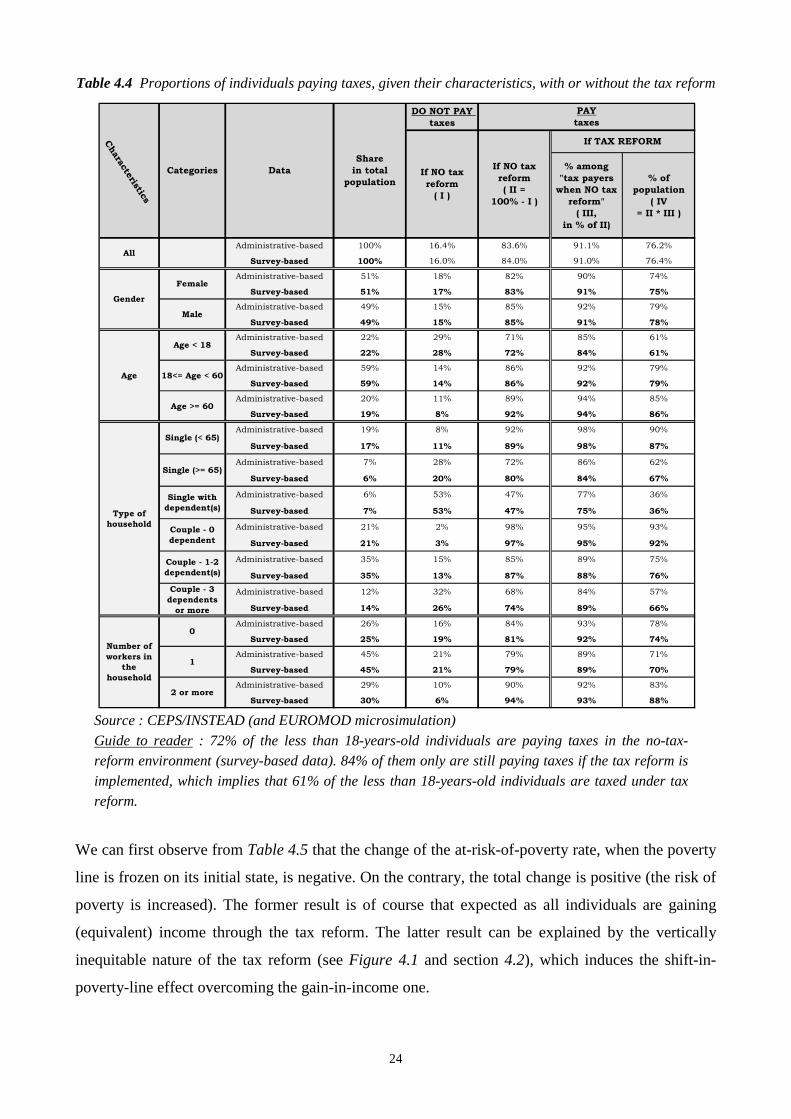
Table 4.4 Proportions of individuals paying taxes, given their characteristics, with or without the tax reform


Guide to reader : 72% of the less than 18-years-old individuals are paying taxes in the no-tax-reform environment (survey-based data). 84% of them only are still paying taxes if the tax reform is

implemented, which implies that 61% of the less than 18-years-old individuals are taxed under tax reform.

We can first observe from Table 4.5 that the change of the at-risk-of-poverty rate, when the poverty

line is frozen on its initial state, is negative. On the contrary, the total change is positive (the risk of

poverty is increased). The former result is of course that expected as all individuals are gaining

(equivalent) income through the tax reform. The latter result can be explained by the vertically

inequitable nature of the tax reform (see Figure 4.1 and section 4.2), which induces the shift-in-

poverty-line effect overcoming the gain-in-income one.

DO NOT PAY

taxes

% among

"tax payers

when NO tax

reform"

( III,

in % of II)

% of

population

( IV

= II * III )

Administrative-based 100% 16.4% 83.6% 91.1% 76.2%

Survey-based 100% 16.0% 84.0% 91.0% 76.4%

Administrative-based 51% 18% 82% 90% 74%

Survey-based 51% 17% 83% 91% 75%


Survey-based 49% 15% 85% 91% 78%


Survey-based 22% 28% 72% 84% 61%


Survey-based 59% 14% 86% 92% 79%


Survey-based 19% 8% 92% 94% 86%


Survey-based 17% 11% 89% 98% 87%


Survey-based 6% 20% 80% 84% 67%


Survey-based 7% 53% 47% 75% 36%


Survey-based 21% 3% 97% 95% 92%


Survey-based 35% 13% 87% 88% 76%


Survey-based 14% 26% 74% 89% 66%


Survey-based 25% 19% 81% 92% 74%


Survey-based 45% 21% 79% 89% 70%


Survey-based 30% 6% 94% 93% 88%

Chara

cte

ristics

Categories Data

Share

in total

populationIf NO tax

reform

( I )

PAY

taxes

If NO tax

reform

( II =

100% - I )

If TAX REFORM

All

Gender

Female

Male

Age

Age < 18

18<= Age < 60

Age >= 60

Number of

workers in

the

household

0

1

2 or more

Type of

household

Single (< 65)

Single (>= 65)

Single with

dependent(s)

Couple - 0

dependent

Couple - 1-2

dependent(s)

Couple - 3

dependents

or more

25

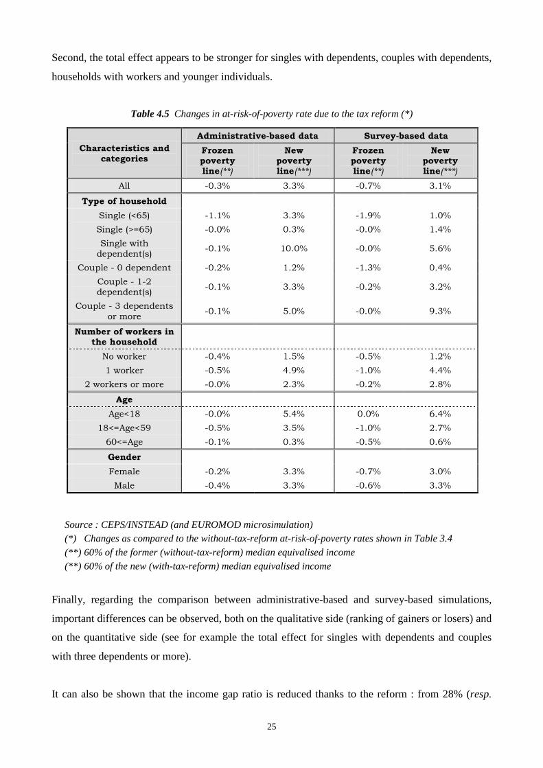
Second, the total effect appears to be stronger for singles with dependents, couples with dependents,

households with workers and younger individuals.

Table 4.5 Changes in at-risk-of-poverty rate due to the tax reform (*)

Source : CEPS/INSTEAD (and EUROMOD microsimulation) (*) Changes as compared to the without-tax-reform at-risk-of-poverty rates shown in Table 3.4

(**) 60% of the former (without-tax-reform) median equivalised income (**) 60% of the new (with-tax-reform) median equivalised income

Finally, regarding the comparison between administrative-based and survey-based simulations,

important differences can be observed, both on the qualitative side (ranking of gainers or losers) and

on the quantitative side (see for example the total effect for singles with dependents and couples

with three dependents or more).

It can also be shown that the income gap ratio is reduced thanks to the reform : from 28% (resp.

Characteristics and categories

Administrative-based data Survey-based data

Frozen poverty line(**)

New poverty line(***)

Frozen poverty line(**)

New poverty line(***)

All -0.3% 3.3% -0.7% 3.1%

Type of household

Single (<65) -1.1% 3.3% -1.9% 1.0%

Single (>=65) -0.0% 0.3% -0.0% 1.4%

Single with dependent(s)

-0.1% 10.0% -0.0% 5.6%

Couple - 0 dependent -0.2% 1.2% -1.3% 0.4%

Couple - 1-2 dependent(s)

-0.1% 3.3% -0.2% 3.2%

Couple - 3 dependents

or more -0.1% 5.0% -0.0% 9.3%

Number of workers in the household

No worker -0.4% 1.5% -0.5% 1.2%

1 worker -0.5% 4.9% -1.0% 4.4%

2 workers or more -0.0% 2.3% -0.2% 2.8%

Age

Age<18 -0.0% 5.4% 0.0% 6.4%

18<=Age<59 -0.5% 3.5% -1.0% 2.7%

60<=Age -0.1% 0.3% -0.5% 0.6%

Gender

Female -0.2% 3.3% -0.7% 3.0%

Male -0.4% 3.3% -0.6% 3.3%

26

18%) down to 24% (resp. 15%) through survey-based (resp. administrative-based) data.

5. CONCLUSIONS

We initiate, through the EUROMOD microsimulation framework, the cross-validation of

administrative data derived from the recently implemented Luxembourg Social Security Data

Warehouse, on the one side, and of the PSELL3/EU-SILC survey data, on the other side.

We choose to work on the 2003 population in Luxembourg in all cases. As a benchmark, the

“without 2001-2002 Luxembourg tax reform” environment is chosen.

Administrative data have some obvious limitations compared to survey data, because in general

administrative data record only information needed for administrative purposes like collecting

social contributions or paying social benefits, whereas the questionnaires for survey data may be

designed specifically for defined research purposes, including a need for standardization and

comparability between countries48. On the other hand, the kind of data provided by the Luxembourg

Social Security Data Warehouse have also some important advantages over survey data, like

completeness49, timeliness, availability of time series of data of different granularity, like yearly or

monthly data50. Moreover, administrative data include some information not available in survey

data, e.g. in relation with health and long term care, cross-border workers (37% of the employment

in 2003, what is essential regarding the tax-benefit system in Luxembourg), etc.

Before comparing the datasets as set up through the EUROMOD input framework, it seems

important to dispose of dissimilarities that we can control for, regarding the target populations and

the lack of precision in some important (income-related) variables. We have then to drop about 6%

of the initial population in both datasets and adapt variables like capital income-related ones which

are missing in the administrative-based dataset.

An important implication is also to adopt the fiscal household as the unit of analysis, rather than the

more usual residence household. This may play a role concerning the comparison of outcomes to

other studies. The fiscal household being included into residence units, this leads to a distribution of

equivalised income which departs from usual ones, with lower values for both means (10% less

when fiscal households, if the benchmark) and medians (-5%). The at-risk-of-poverty rate and the

gain or loss for the different categories of population are also affected.

27

Regarding several non-monetary characteristics, like the age classes and the types of households,

the two EUROMOD input datasets appear to be satisfactorily similar. For monetary characteristics a

first discordance is observed, mainly stemming from a gap in primary income which is, on average,

7% lower in administrative-based data, an observation to be further explored. The difference in

primary income implies downstream effects on equivalised income.

Under the benchmark environment, the Gini coefficient and other inequality indices most often

show a similar distribution of equivalised income in both datasets. Nevertheless, regarding the

leftist part of the distribution, the at-risk-of-poverty rates are higher through survey-based data, for

all categories under study51. Whatever the dataset under consideration, usually more at-risk-of-

poverty categories are shown up, like “singles with dependent(s)” and the members of households

where nobody is working. Nevertheless, next to the qualitative comparison of outcomes, a few

striking discrepancies appear, for example for the “singles with dependent(s)” who are marked

twice more at risk of poverty through survey-based data in the without-tax-reform environment.

It is shown that the 2001-2002 tax reform in Luxembourg results, for the resident population of

2003, in a rise of mean equivalised income by 6%. More specifically, the elderly and singles

without dependent(s) seem to experience better gains, on average, than other categories in the

corresponding typology. The higher the income, the higher the relative gains, whatever the category

under consideration. The average gain for the highest decile of the population is about 9%, to be

compared with less than 1% for the lowest decile, whatever the dataset. The Gini coefficient, higher

with the reform, follows. This increase in inequality due to the reform is shown to result from a

magnitude effect, i.e. the drop in the average rate of taxation, and not from the progressivity which

is augmented, indeed. The at-risk-of-poverty rates of the different categories are increasing. But

some, like singles with dependents and couples with three dependents or more are experiencing a

rise which may considerably differ in intensity between administrative-based and survey-based

data.

On the whole, we can conclude at a satisfactory “proximity” (e.g. a statistical compatibility as

assessed through confidence intervals) between the administrative-based and survey-based data,

whether as input data for EUROMOD or as far as the effects of the 2001-2002 tax reform are

concerned. Nevertheless, this robustness in the results regarding the source data is less observed

when some monetary characteristics and the at-risk-of-poverty rates (whatever absolute levels or

changes due to the tax reform) are considered. Even if the change of the average at-risk-of-poverty

rate is similar with the two datasets, outcomes for specific categories may strongly differ52.

28

Of course, this promising cross-validation outcome lies on the treatment we have chosen to impose

to the initial datasets for making them targeting closer populations and getting rid of the effect of

some income-related missing or unevenly biased variables.

The next step might be to further explore these questions, especially on the administrative side or

regarding the income measurement, in order to make those methodology-based arrangements

essentially no longer necessary. An important extension concerning administrative data in

Luxembourg would also be to properly deal with (postal) addresses, e.g. in order to make residence

and institutional households identifiable and spatial analysis feasible.

BIBLIOGRAPHY

Atkinson E., Cantillon B., Marlier E. and Nolan B. (2002), Social indicators : The EU and Social

Inclusion, New York, Oxford University Press.

Berger F., Hausman P., Jeandidier B., Ray J.-C., Reinstadler A. et Zanardelli M. (2002), Les effets

redistributifs de la politique familiale, Etude réalisée pour le compte du Ministère de la Famille du Grand-Duché de Luxembourg, CEPS/INSTEAD

Callan T. and Walsh J. (2006), Assessing the Impact of Tax/Transfer Policy Changes on poverty : Methodological Issues and Some European Evidence, EUROMOD Working paper, EM1/06

Essama-Nssah B. (2000), Inégalité, pauvreté et bien-être social, Bruxelles, De Boeck Université

Figari F., Levy H. and Sutherland H. (2007), Using the EU-SILC for policy simulation : propects, some limitations and suggestions, EUROMOD Working paper, EM1/07

Fuchs M. and Lietz C. (2007), Effect of changes in tax/benefit policies in Austria 1998-2005, EUROMOD Working paper, EM3/07

Immervoll (2000) The Impact of Inflation on Income Tax and Social Insurance Contributions in Europe, EUROMOD Working paper, EM2/00

Immervoll H., Levy H., Lietz C., Mantovani D. and Sutherland H. (2006), The sensitivity of poverty rates to macro-level changes in the European Union, Cambridge Journal of Economics, 30, 181-199

Lambert, P.J. (1993), The distribution and redistribution of income – a mathematical analysis, 2nd Edition, Manchester University Press

Marlier E., Atkinson E., Cantillon B. and Nolan B. (2006), the EU and social inclusion : Facing the

challenges, Bristol, Policy Press.

Nordberg L. (2003), An analysis of the effects of using interview versus register data in income distribution analysis based on the Finnish ECHP-surveys in 1996 and 2000, CHINTEX Working

Paper #15, Abo Akademi university.

29

Nordberg L. and Pentillä I. (2001), Interview and Register Data in income Distribution Analysis.

Experiences from the Finnish European Community Household Panel in 1996, Reviews 2000/9, Helsinki, Statistics Finland

Sutherland, H. (Ed) (2001), EUROMOD : an integrated European Benefit-tax model, Final report, EUROMOD Working paper, EM9/01

APPENDIX : THE TAX SYSTEM IN LUXEMBOURG AND THE 2001-2002 REFORM

In this appendix, we describe the main characteristics of the tax system in Luxembourg and the

modalities of the 2001-2002 reform. We focus on elements relevant to the present analysis only.

A.1 The tax system in Luxembourg

In Luxembourg, the tax unit is the “family” which might not include all members of a “residence

household”53. To belong to the same family, you must either be (official) spouse or a dependent

child. Two cohabiting but non-spouse persons are then members of separate tax units. A “child”

belongs to his/her parents’ tax unit if unmarried and less than 21 years old. As soon as married, a

son/daughter enters his/her own tax unit. The same prevails if a person is older than 21 years and is

neither a student any longer nor a disabled person. Of course, the set of rules includes many other

aspects, related to the questions of “earnings” of dependent children, children living part-time only

with their parents, status changing during the civil year, spouses separating/being divorced, etc.

These questions, although essential to the system as a whole, are not discussed here because they

are not necessary for a clear understanding of the present analysis.

The tax system on income being progressive, it is important to know how the tax basis is defined.

The taxable income is firstly involving the yearly gross earnings of all the members of the family

(as defined earlier) : wages, business profits, income from farming and forestry/self-

employment/pensions, investment and property incomes, etc. Social contributions and several tax

allowances (e.g. for travel expenses or if a lone parent) are then deducted from gross amounts to

define the adjusted taxable income. The adjusted taxable income is rounded54 before applying the

tax schedule (brackets and marginal rates) which is described in Table A.1 for the years 2000 up to

2003. This tax schedule is used depending on the tax class the tax payer belongs to : class 1, class

1a or class 2. The tax class is defined given both family and individual characteristics of the tax

payer, as shown in Table A.2.

30

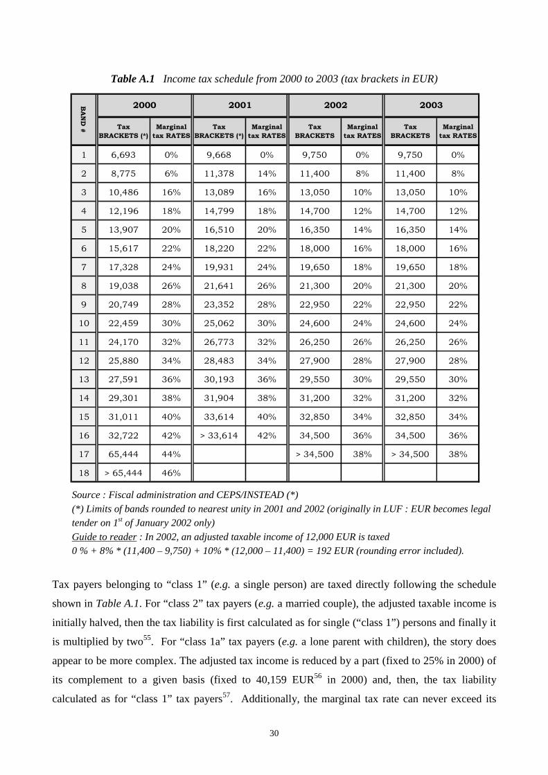
Table A.1 Income tax schedule from 2000 to 2003 (tax brackets in EUR)

Source : Fiscal administration and CEPS/INSTEAD (*)

(*) Limits of bands rounded to nearest unity in 2001 and 2002 (originally in LUF : EUR becomes legal tender on 1st of January 2002 only)

Guide to reader : In 2002, an adjusted taxable income of 12,000 EUR is taxed 0 % + 8% * (11,400 – 9,750) + 10% * (12,000 – 11,400) = 192 EUR (rounding error included).

Tax payers belonging to “class 1” (e.g. a single person) are taxed directly following the schedule

shown in Table A.1. For “class 2” tax payers (e.g. a married couple), the adjusted taxable income is

initially halved, then the tax liability is first calculated as for single (“class 1”) persons and finally it

is multiplied by two55. For “class 1a” tax payers (e.g. a lone parent with children), the story does

appear to be more complex. The adjusted tax income is reduced by a part (fixed to 25% in 2000) of

its complement to a given basis (fixed to 40,159 EUR56 in 2000) and, then, the tax liability

calculated as for “class 1” tax payers57. Additionally, the marginal tax rate can never exceed its

Tax

BRACKETS (*)

Marginal

tax RATES

Tax

BRACKETS (*)

Marginal

tax RATES

Tax

BRACKETS

Marginal

tax RATES

Tax

BRACKETS

Marginal

tax RATES

1 6,693 0% 9,668 0% 9,750 0% 9,750 0%

2 8,775 6% 11,378 14% 11,400 8% 11,400 8%

3 10,486 16% 13,089 16% 13,050 10% 13,050 10%

4 12,196 18% 14,799 18% 14,700 12% 14,700 12%

5 13,907 20% 16,510 20% 16,350 14% 16,350 14%

6 15,617 22% 18,220 22% 18,000 16% 18,000 16%

7 17,328 24% 19,931 24% 19,650 18% 19,650 18%

8 19,038 26% 21,641 26% 21,300 20% 21,300 20%

9 20,749 28% 23,352 28% 22,950 22% 22,950 22%

10 22,459 30% 25,062 30% 24,600 24% 24,600 24%

11 24,170 32% 26,773 32% 26,250 26% 26,250 26%

12 25,880 34% 28,483 34% 27,900 28% 27,900 28%

13 27,591 36% 30,193 36% 29,550 30% 29,550 30%

14 29,301 38% 31,904 38% 31,200 32% 31,200 32%

15 31,011 40% 33,614 40% 32,850 34% 32,850 34%

16 32,722 42% > 33,614 42% 34,500 36% 34,500 36%

17 65,444 44% > 34,500 38% > 34,500 38%

18 > 65,444 46%

2000 2001 2002 2003BA

ND

#

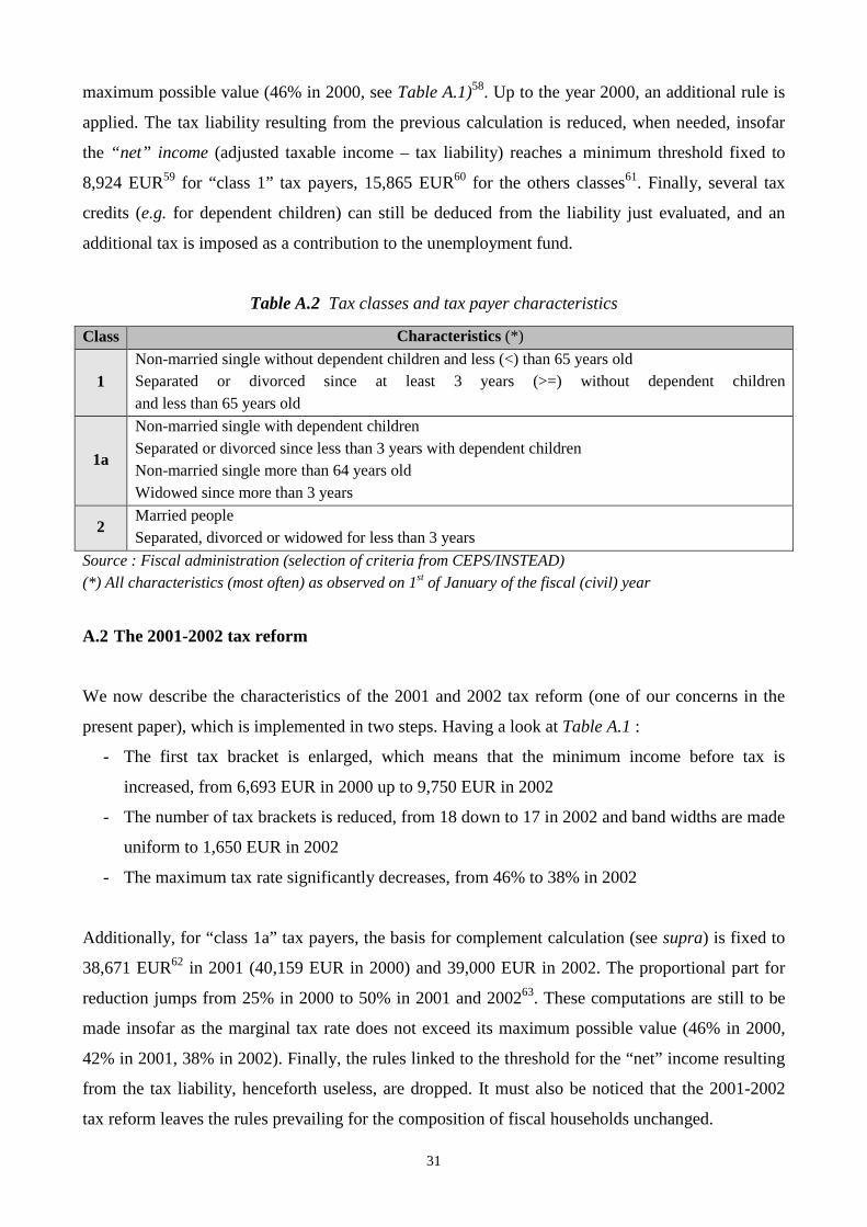
31

maximum possible value (46% in 2000, see Table A.1)58. Up to the year 2000, an additional rule is

applied. The tax liability resulting from the previous calculation is reduced, when needed, insofar

the “net” income (adjusted taxable income – tax liability) reaches a minimum threshold fixed to

8,924 EUR59 for “class 1” tax payers, 15,865 EUR60 for the others classes61. Finally, several tax

credits (e.g. for dependent children) can still be deduced from the liability just evaluated, and an

additional tax is imposed as a contribution to the unemployment fund.

Table A.2 Tax classes and tax payer characteristics

Class Characteristics (*)

1 Non-married single without dependent children and less (<) than 65 years old Separated or divorced since at least 3 years (>=) without dependent children and less than 65 years old

1a

Non-married single with dependent children Separated or divorced since less than 3 years with dependent children Non-married single more than 64 years old Widowed since more than 3 years

2 Married people Separated, divorced or widowed for less than 3 years

Source : Fiscal administration (selection of criteria from CEPS/INSTEAD) (*) All characteristics (most often) as observed on 1st of January of the fiscal (civil) year

A.2 The 2001-2002 tax reform

We now describe the characteristics of the 2001 and 2002 tax reform (one of our concerns in the

present paper), which is implemented in two steps. Having a look at Table A.1 :

- The first tax bracket is enlarged, which means that the minimum income before tax is

increased, from 6,693 EUR in 2000 up to 9,750 EUR in 2002

- The number of tax brackets is reduced, from 18 down to 17 in 2002 and band widths are made

uniform to 1,650 EUR in 2002

- The maximum tax rate significantly decreases, from 46% to 38% in 2002

Additionally, for “class 1a” tax payers, the basis for complement calculation (see supra) is fixed to

38,671 EUR62 in 2001 (40,159 EUR in 2000) and 39,000 EUR in 2002. The proportional part for

reduction jumps from 25% in 2000 to 50% in 2001 and 200263. These computations are still to be

made insofar as the marginal tax rate does not exceed its maximum possible value (46% in 2000,

42% in 2001, 38% in 2002). Finally, the rules linked to the threshold for the “net” income resulting

from the tax liability, henceforth useless, are dropped. It must also be noticed that the 2001-2002

tax reform leaves the rules prevailing for the composition of fiscal households unchanged.

32

Figure A.1 Impact of the 2001-2002 tax reform

on the average rate of tax on income, given the tax class


Figure A.1 shows how taxes are changing through the reform, given the adjusted taxable income

and the tax class to be considered. The gain for tax payers is rather high, about a 7 % drop in the

average tax rate for all classes when an adjusted taxable income of 50,000 EUR / year (idem for

“class 1” tax payers if an income of 30,000 EUR, 8% for “class 1a”, 5% for “class 2”).

ENDNOTES

3 Source : STATEC - National statistical institute of Luxembourg (through

http://www.statistiques.public.lu).

4 For a detailed presentation of social indicators, see Atkinson et al. (2002) and Marlier et al. (2006).

5 http://www.iser.essex.ac.uk/msu/emod/

6 For a comparison between outcomes from interview and register data, see also e.g. Nordberg (2003)

and Nordberg and Pentillä (2001), for Finland.

7 “Panel Socio-Economique Liewen zu Lëtzebuerg” (see http://www.ceps.lu/).

8 EU-SILC is an instrument aiming at collecting timely and comparable cross-sectional and

longitudinal multidimensional microdata on income, poverty, social exclusion and living conditions

(see http://epp.eurostat.ec.europa.eu/).

9 See http://www.statec.public.lu

10 Inspection Générale de la Sécurité Sociale (see http://www.mss.public.lu/).

11 MSW = 1368.74 EUR / month as on 1st of January 2003.

0%

5%

10%

15%

20%

25%

30%

35%

40%

Avera

ge t

ax r

ate

Adjusted taxable income (EUR /year)

Class 1 - 2000

Class 1 - 2002

Class 1a - 2000

Class 1a - 2002

Class 2 - 2000

Class 2 - 2002

33

12 A track for overcoming the problem would be to deal with postal addresses, after improvement in

their normalization.

13 Either married all along the year, or married during the (civil) year, or divorced during the year.

14 If unmarried parents, the child goes to his mother’s household, unless an explicit demand from the

mother to link the child with his father concerning the family benefits. If born during the year, or

when family benefits come to an end during the (civil) year, a child is still linked to his parents’

household.

15 Information for non-residents is partially available in the Data Warehouse.

16 Total disposable income = (earnings – social contributions – taxes + social benefits) summed up over

all members of the household.

17 2,110 = 2,110 / 1.0

18 1,000 = 1,800 / 1.8

19 Both the household disposable income (to be attributed to each member within the household) and

the individual equivalent weight are unambiguously lower in a “fiscal” framework, compared to the

“residence” one. But the impact on the individual ratio is qualitatively unknown ex ante (see example

in Table 2.2), as well as the average evolution of the equivalised income throughout the population.

20 When the weighting of cases (designed for better fitting the Luxembourg population) is implemented

/ taken into account.

21 Of course, the adaptation/selection procedure just described may help. Moreover, the weighting

process of the survey data is also based on administrative data sources partially overlapping our

administrative-based dataset. Nevertheless, this was not at all a priori a guarantee for comparability

for fiscal households.

22 Primary income = gross employment and self-employment income + gross investment and property

income (excluded from results in Table 3.3, for comparability reasons) + maintenance payments +

gross private pension benefits (low, on average, in Luxembourg) + apprentice income.

23 Nordberg (2003) gets for Finland a level of « earned income » (close to our « primary income”) lower for

register data in 1995 but higher in 1999.

24 If a confidence level of 99%, the conclusion does not change.

25 For example, as a proxy for “institutional households”, all individuals more than 75 years old and

mentioned as “single without dependent” are dropped from both the administrative-based dataset

(“institutional households” included in initial data) and survey-based data (for symmetry reasons).

26 The mean primary income goes from 1,384 up to 1,464 on the administrative-side, from 1,493 up to

1,539 on the survey-side, with, for the latter, a confidence interval changing to [1,459 - 1,619].

27 This information is partially available in the input datasets. While simulating through EUROMOD,

we avoid the question of non-take-ups and, on top of that, dissimilarities due to differing levels of

non-take-ups that might be observed in administrative-based and survey-based data.

28 The Atkinson inequality index can be expressed as �� 1 � �� ∑ ��

� ��

��

, where n is the

number of individuals, xi is the income level, � the average income and � the inequality aversion coefficient. It takes a value between 0 (minimum inequality) and 1 and can be interpreted in terms of

social welfare : it shows that part of total income which might be saved, while keeping the social

welfare (associated to the Atkinson index) unchanged and distributing the remaining disposable

income equally. See Essama (2000) and Lambert (1993).

29 The Gini coefficient takes a value between 0 (minimum inequality) and 1. If we define the social

welfare as �� ∑ ∑ !"#$�� , �&'&� , then it can be shown that �� 1 � )�, where n is the

number of individuals, xi/j is the income level, � the average income and G the Gini inequality index.

See Essama (2000) and Lambert (1993).

30 These would be fully compatible in all cases if a 99% confidence interval.

31 A decomposition of inequality indices by population sub-group could also enlighten the question.

32 The 95% confidence interval for the average poverty rate through survey-based data is

[8.4% - 10.7%].

33 Only couples with 3 dependents or more are signaled less at-risk-of-poverty through survey-based

than administrative-based data.

34

34 Table 3.5 helps in understanding the reason why, concerning the whole population. With ratio of

mean income between the first decile (nearby the poverty line) and the fifth one (close to median

income) of 0.55 (= 47% / 85%) in administrative-based data, to be compared with 0.46 for the

survey-based data, we can expect that fewer members of the first decile in the administrative-based

data are to be trapped below the poverty line.

35 The Foster-Greer-Thorbecke poverty index with parameter 1, which is the product of the poverty rate

and the income gap ratio, is shown to be 0.027 through survey-based data (resp. 0.013 through

administrative-based data), leading to an income gap ratio of 0.027/0.096 = 28% (resp. 18%). The

income gap ratio = 1 – (Mean income of the “poor”/Poverty line) : it refers to the extent to which the

incomes of the poor lie below the poverty line.

36 A “Single with dependent(s)” is most often a single parent with dependent child(ren). See Table 3.1.

37 See Callan and Walsh (2006) for a proposal of alternative benchmarks, including a “distributional

neutral policy”, mainly appropriate when a comparison between countries.

38 As it is presently designed, neither feedback effects through prices or budget constraints, nor

behavioral answers. Moreover, EUROMOD is static which means that the time dimension (hence

links through time) is not included in the model.

39 See section 3.3.

40 Vertical redistribution consists in reducing inequalities of equivalised income between households

who have the same structure, but a different income level.

41 Horizontal redistribution consists in reducing inequalities of equivalised income between households

who have the same income level, but a different structure.

42 The increase in progressivity can be explained by an enlargement of the first tax bracket

(tax rate = 0%) which overcomes, regarding the measurement of progressivity through the Kakwani

index, the effect of reducing the marginal tax rates for higher income levels.

43 We could also compare mean income for deciles determined from the income distribution when no

tax reform, on one side, to deciles determined with the tax reform implemented, on the other side

(the result is not reported in the paper but available on demand). We preferred the above

presentation which leaves the members of the deciles unchanged.

44 There is no gain for first two deciles of more-than-65-years-old singles, which means that the

members of those categories are taxed neither with nor without the reform. As can be seen from

Table 3.5, the mean equivalised income (which is simply disposable income, for singles) for second

decile is about 1,300 EUR / month or 15,600 EUR / year for more-than-65-years-old singles, which

is below the threshold for taxable income for “class 1a” tax payers (15,865 EUR in 2000, above later

on).

45 One counterexample is to be found for 2-workers’ households, between first and second deciles, in

survey-data only.

46 For example, singles with dependent(s) and households where nobody or one person only is working

show an equivalised income more concentrated on the first deciles, compared to average (see Table

3.4), a first condition for lower taxation.

47 For example, more-than-65-years-old singles are benefitting from the advantageous “class 1a”

taxation when non-married (see appendix). The Luxembourg tax-benefit system is also exhibiting an

important “family advantage” (Berger et al., 2002).

48 Due to the tax reform, the poverty line is increasing from 1,188 EUR (see Table 3.3) to 1,254 EUR

(+ 5.6%) when survey-based data, from 1,138 EUR to 1,199 EUR (+ 5.4%) when administrative-based

data.

49 See also Immervoll et al. (2006).

50 See Figari et al. (2007).

51 Which implies that working on categories is easier than with survey-based data where an

appropriate procedure for the weighting of cases may be necessary.

52 It may be important to know, as far as the tax-benefit system is concerned, how the value of a

variable evolves during the year (e.g. in Luxembourg : the marital status).

53 Out of the income characteristic, we have chosen to focus our attention on typologies based on the

age (<18, >= 60, others), the gender, the number of workers within the (fiscal) household and the

type of household (single < 65, single 65+, single with dependents, couples with 0/1-2/3

dependents).

35

54 Several determinants play indeed a role when categories are compared and cannot always be easily

disentangled : the overall distribution of disposable income, the composition of households and the

characteristics of the tax-benefit system. This complexity explains why impacts on categories of

populations, in terms of relative gain and ranking, may depend on the criteria shown up.

55 A residence household is defined as all persons “living together” at the same address.

56 To the nearest lower multiple of EUR 50, from 2002 on.

57 Example : In 2002, a married couple with adjusted taxable income = 30,000 EUR will be attributed a

tax liability of 1,074 EUR = 2 * 537 EUR (tax liability for an income of 15,000 EUR when “single”

without children).

58 1,620,000 LUF (1 EUR = 40.3399 LUF).

59 Example : a lone parent with children whose taxable income is 30,000 EUR is attributed a tax

liability of 4,970 EUR [tax liability when a “class 1” tax payer whose income is 30,000 – 25% *

(40,159 – 30,000) = 27,460 EUR]. NB : the “complement” calculation is performed only if the adjusted

taxable income is less than the basis (40,159 EUR). Moreover, if leading to a negative outcome, the

value is set to “0”.

60 Formally, this means that when an increase of income by 1000 EUR, the supplement in tax liability

can never exceed, in 2000, 460 EUR for “class 1a” tax payers.

61 360,000 LUF.

62 640,000 LUF.

63 Example : a young single without children (hence « class 1 ») whose adjusted tax income is 9,000

EUR in 2000 should have paid, given the schedule for his class, a tax of 161 EUR. Nevertheless, this

would result in a “net” income of 9,000 – 161 = 8,839 EUR, which is below the threshold of 8,924

EUR, hence leading to a reduction of the tax down to 76 EUR and a net of 8,924 EUR.

64 1,560,000 LUF.

65 Example : a lone parent (with children) whose taxable income is 30,000 EUR in 2002 is now

attributed a tax liability of 1,125 EUR [tax liability when a “class 1” tax payer whose income is

30,000 – 50% * (39,000 – 30,000) = 25,500 EUR].

Cross-validating administrative and survey datasets through microsimulation

Documents