Cross-country Convergence and Growth: Evidence from

1

Cross-country Convergence and Growth:

Evidence from Nonparametric and Semiparametric Analysis

Kui-Wai Li a,* and Xianbo Zhoub a City University of Hong Kong, Hong Kong

b Lingnan College, Sun Yat-Sen University, China

Paper submitted to

APEC Study Center Consortium Conference

September 22 – 23, 2011

San Francisco, USA

2

Cross-country Convergence and Growth:

Evidence from Nonparametric and Semiparametric Analysis

Kui-Wai Li a,* and Xianbo Zhoub a City University of Hong Kong, Hong Kong

b Lingnan College, Sun Yat-Sen University, China

Abstract

This article studies the absolute and conditional convergence of real GDP per capita

among 164 world economies over the sample period of 1970-2006. The data-driven

model specification tests justify the use of nonparametric and semiparametric models.

The estimation results show that control variables play a negative/positive channel effect

in the growth convergence for poor/developed economies. The absolute convergence

hypothesis tends to hold only for the economies with low development levels, but the

conditional convergence hypothesis tends to hold for all the economies.

Keywords: convergence, nonparametric, semiparametric, growth

JEL Classifications: C14, F43, O11, O40

____

* Corresponding author: Kui-Wai Li, Department of Economics and Finance, City University of Hong Kong. Tel.: +852 3442 8805; Fax: +852 3442 0195; E-mail: [email protected]

3

I Introduction

In the growth and development literature, parametric regression analysis has

empirically been used to test the convergence hypothesis that poorer economies will

catch up with wealthier economies (Baumol, 1986; Barro and Sala-i-Martin, 1992; Islam,

1995; Evans and Kim, 2005). Much of the empirical research has concentrated on

whether per capita income growth converges once structural differences across

economies have been controlled for. In the parametric regression, a negative parametric

estimate of the coefficient on the initial income is interpreted as evidence of convergence.

Different parametric methodologies based on exogenous and endogenous growth models

have been employed in studying income convergence. Some studies conducted panel unit

root test on the convergence hypothesis (Quah, 1994; Levin and Lin, 1993; Im et al.,

1997). Others used the system-generalized method of moments for the dynamic panel

data model (Bond et al. 2001) to show that earlier results might be seriously biased due to

weakness of the instruments in the first-differenced generalized method of moments

approach. The convergence debate is summarized and analyzed in Islam (2003).

A key assumption in the conventional studies with parametric models is that

cross-country growth is linear with identical rate of convergence across countries and the

convergence is only tested according to the parametric estimate of the coefficient on the

initial income. However, as some new growth theories (Azariadis and Drazen, 1990;

Durlauf and Johnson, 1995) have shown, cross-country growth can be non-linear and is

characterized by multiple steady states and the implied rates of convergence differ

between different groups of economies.

In contrast to the above parametric studies, nonparametric approaches that

pre-specify neither the income distribution form nor the functional form of the regression

4

function have been applied to the study of convergence. For example, Bianchi (1997)

studied the convergence hypotheses among 119 countries by means of bootstrap

multimodality tests and nonparametric density estimation techniques and supports the

clustering and stratification of growth patterns over time. Wang (2004) applied a

nonparametric approach to test the convergence hypothesis of the income distribution

across the 59 provinces and states in the U.S. and Canada and finds club convergence or

multi-modality of the per capita income over the sample period. Lauruni et al. (2005)

employed nonparametric methodology to analyze the evolution of relative per capita

income distribution of Brazilian municipalities over the period 1970-1996. In a more

recent literature, Juessen (2009) used nonparametric estimation to study GDP

convergence in the labor market across different regions in Germany for the period

1992-2004, and the bimodality result indicated sizeable disparities between regions.

Although nonparametric estimation relaxes the assumption on the same rate of

convergence across countries, these nonparametric analyses have excluded other steady

state growth determinants and have concentrated on the empirical research of the absolute

convergence.

To control for structural differences across countries in the steady state, recent

empirical research used semiparametric methods to test the conditional convergence

hypothesis and estimated the implied rate of convergence as a function of the initial

income. Kumer and Ullah (2000) developed a local linear instrumental variable method

with a kernel weight function to estimate the smooth varying coefficient function and

applied it to estimate the speed of convergence of a panel of cross-countries per capita

output. Dobson et al. (2003) presented a brief semiparametric analysis on the

cross-country convergence by simply pooling the data for 103 countries covering the

5

period 1960-1990 and provided evidence for nonlinear convergence. Azomahou et al.

(2011) applied a semiparametric partially linear model to approximate the relationship

between the growth and initial GDP per capita across European regions and confirmed

the nonlinearity in the convergence process.

The growing popularity of nonparametric and semiparametric approaches stems

from their ability to relax functional form assumptions in regression model and let the

data determine the convergence process (Henderson et al., 2008). The nonlinearity and

the heterogeneity in structural economies can be accounted for since there is little prior

knowledge on a particular convergence process. A more general data-based specification

of the functional form is robust to the functional misspecification for convergence.

Therefore, nonparametric and semiparametric models can be more flexible than

parametric models in describing the nonlinearity in the convergence process and the

multiple steady states in the economy.

In light of the nonlinearity in the convergence process and the heterogeneity of

cross-country structural economies, this article proposes the use of both nonparametric

and semiparametric panel data models to study absolute and conditional convergence,

respectively. By using an unbalanced panel data set of 164 world economies over the

period 1970-2006, this article examines whether differences in macroeconomic and

institutional factors, endowments, and other country characteristics have played a role in

per capita income growth and convergence among world economies. As we know, panel

data analysis on the income convergence can incorporate heterogeneity across economies.

The fixed and random effects are often specified in the growth model for the

unobservable heterogeneity in the economies. There is no agreement as to which kind of

6

effects is more suitable to enter into the model1. However, in order to obtain consistent

estimates for the nonparametric function of the lagged output and the speed of

convergence, no matter whether the individual effect is random or fixed, we apply the

fixed-effects specification in our nonparametric and semiparametric models, as suggested

by Henderson et al. (2008).

Section II describes the data and variables. Section III presents the estimation of the

nonparametric and semiparametric models and the model specification tests with

unbalanced panel data. Section VI reports empirical estimation and analysis. Section V

presents the testing results which justify the semiparametric and nonparametric model

specification. Section V concludes the paper.

II Data and Selection of Variables

We include in the convergence models a total of nine control variables in the vector

of characteristics in order to reflect differences in the steady state equilibrium and to

capture a variety of socio-economic factors. These nine variables are: investment

(investment share of real GDP per capita), inflation (annual percentage of GDP deflator),

government size (government expenditure share of real GDP per capita), trade

(percentage share of trade in GDP), foreign direct investment (percentage share of net

foreign direct investment in GDP), life expectancy, urbanization (share of urban people in

total population), private credit share (domestic credit to private sector as a percentage of

1 When the individual effect is independent of the regressors, the estimation of both the random-effects

model and the fixed-effects model is consistent with each other, except that the random effects estimator is

more efficient. However, when the individual effect is correlated with any of the regressors, the random

effects estimator is biased and inconsistent whereas the fixed effects estimator still leads to consistent

estimates and is appropriate for the estimation of regression functions.

7

GDP), and carbon dioxide emission (carbon dioxide emission per capita).

The data for the real GDP per capita (gdpc) are in 2005 constant prices derived from

growth rates of consumption, government expenditure and investment. We include

investment (ki) as a control variable since it has been one of the determinants in the

conventional Solow growth model. The rate of inflation (deflator) acts as a proxy for

macroeconomic stability with the intention to test the hypothesis of the negative effect to

income growth found in several studies (Fischer, 1993; Barro, 1995). Government size

(kg) is used to proxy an institutional indicator and to test if a larger government size was

likely to harm growth, as shown in Iradian (2003, 2005). Trade openness (trade) and

foreign direct investment (fdi) are included in our analysis as trade has always been seen

as an important catalyst for economic growth and foreign direct investments generate

increasing returns in production through positive externalities and spillover effects

(Frankel and Romer, 1999; Dollar and Kraay, 2001; Makki and Somwaru, 2004). Health

in the form of life expectancy (life) has appeared in many cross-country growth

regressions and has been generally found to have a significant positive effect on the rate

of economic growth (Bloom and Canning, 2000; Bloom et al., 2001). Life expectancy is

thus used to indicate whether increased expenditures on health are justified on the

grounds of their impact on economic growth. Urbanization (urban) has been viewed

necessary for achieving high growth, high income, increased productivity and efficiency

through specialization, diffusion of knowledge, size and scale (Annez and Buckley, 2009;

Duranton, 2009; Quigley, 2009). However, urbanization may also deter firms from

locating in larger cities due to negative spillovers including congestion and high land

rents, leading to dampening effect on economic growth. Urbanization is included in our

analysis to provide evidence if its progress supports income growth. The remaining two

8

variables of carbon dioxide emission (co2) and private credit share (credit) are used to

capture the environmental issue and level of financial development, respectively.

The data are sourced from the Penn World Tables, World Development Indicators

and the United Nations. The unbalanced panel dataset (see Appendix) used in the analysis

contains 4,450 observations on 164 world economies for the period 1970-2006, with each

country containing at least two-year data to fit in with our nonparametric estimation.

III Nonparametric Models and Specification Test

Recent empirical studies using the semiparametric approach have challenged

parametric specifications that stemmed from the linearity in the convergence process.

This article re-examines the convergence process by specifying nonparametrc and

semiparametric panel data models. Nonparametric method relaxes the assumption of the

identical speed of convergence implied in parametric models and allows convergence to

be related to the initial economic development level. The generated flexibility allows the

data of the economies to determine the functional form of the initial income. We will also

present model specification tests which show that our models are justified in studying the

convergence process.

The nonparametric panel data model with country-specific fixed effects is specified

as

, 1 , 1ln( ) ln( ) (ln( )) ,it i t i t i itgdpc gdpc g gdpc u v− −− = + + (1)

where 1,2, , ; 1,2, , ,it m i n= =L L ln( )itgdpc is the logarithm of real GDP per capita

and the functional form of ( )g ⋅ is not specified and , 1ln( ) ln( )it i tgdpc gdpc −− is the

growth rate of real GDP per capita. Each country i has im observations. For consistent

9

estimation of ( )g ⋅ , we specify a nonparametric estimation of the fixed effects model,

that is, the individual effects iu are fixed effects which are allowed to be correlated with

, 1ln( )i tgdpc − . The error term itv is assumed to be i.i.d. with a zero mean and a finite

variance, and is mean-independent of , 1ln( )i tgdpc − , namely , 1( | ln( )) 0it i tE v gdpc − = .

The semiparametric panel data model with country-specific fixed effects is the

semiparametric counterpart of Model (1) with control variables. It is specified as

', 1 , 1ln( ) ln( ) (ln( )) ,it i t i t it i itgdpc gdpc g gdpc x u vβ− −− = + + + (2)

where itx is the vector of the logarithms of control variables accounting for differences

in investment, economic environment including rate of inflation, trade openness and

intensity of foreign direct investment, degree of financial market development indicated

by private credit share, as well as social and human indicators including government

consumption share, life expectancy, carbon dioxide emission and urbanization. The

assumptions of the error term itv are similar to those in Model (1), and that they are i.i.d.

with a zero mean and a finite variance, and is mean-independent of , 1ln( )i tgdpc − ,

namely , 1( | ln( )) 0it i tE v gdpc − = . The regression function ( )g ⋅ of Model (2) and the

derivative of ( )g ⋅ are the focus in our estimation. If ( )g ⋅ has a known function form

with unknown parameters, Models (1) and (2) become parametric models, with the

former used to study absolute convergence and the latter used to study conditional

convergence.

It follows from the neoclassical growth model that the growth rate is inversely

correlated to the distance from the steady-state value. According to Rassekh (1998), the

speed of convergence λ can be expressed as

10

*ln( ) ln( ) ln( ) .itit

d gdpc gdpc gdpcdt

γ ⎡ ⎤= −⎣ ⎦

The rate is inversely correlated with the distance between the actual GDP per capita

ln( )itgdpc and the final value *ln( )gdpc in steady state. If the convergence rate is

assumed to be a constant, we can write the convergence model in a stochastic form as

*, 1 , 1ln( ) ln( ) (1 ) ln( ) (1 ) ln( )it i t i t i itgdpc gdpc e gdpc e gdpc u vλ λ− −− −− = − − + − + + ,

denoted as *

, 1 , 1ln( ) ln( ) ln( ) ln( ) ,it i t i t i itgdpc gdpc gdpc gdpc u vβ β− −− = − + +

where *gdpc is the income level at the steady state which can be determined by other

control variables of the economy, andβ is the derivative of the growth rate with respect

to , 1ln( )i tgdpc − and can be estimated by regression. Then the speed of convergenceλ

can be calculated by

ln(1 ).λ β= − + (3)

Correspondingly, for Model (1) and Model (2), we replaceβ in (3) by the derivative

function of the growth rate with respect to , 1ln( )i tgdpc − and define the speed of

convergence λ as a function of ln( )gdpc :

(ln( )) ln(1 '(ln( ))),gdpc g gdpcλ = − + (4)

where '( )g ⋅ is the first derivative function of ( )g ⋅ . Therefore, λ is interpreted as the

convergence rate of the economy to the steady-state and this speed may be different in

different initial development level in the economy.

Nonparametric model (1) and semiparametric model (2) can be estimated by the

iterative procedures modified for the unbalanced panel data models in Henderson et al.

(2008). We use the same notation as those in Henderson et al. (2008) to illustrate our

11

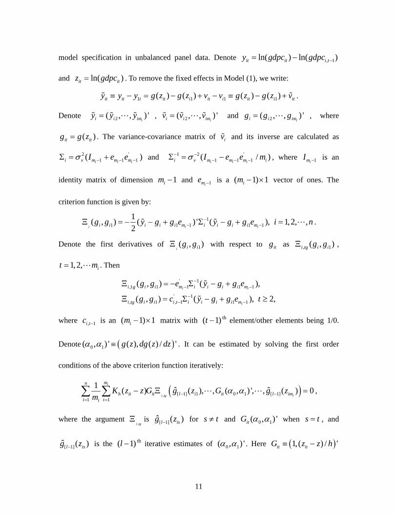
model specification in unbalanced panel data. Denote , 1ln( ) ln( )it it i ty gdpc gdpc −= −

and ln( )it itz gdpc= . To remove the fixed effects in Model (1), we write:

1 1 1 1( ) ( ) ( ) ( )it it t it i it i it i ity y y g z g z v v g z g z v≡ − = − + − ≡ − +% % .

Denote 2( , , ) 'ii i imy y y=% % %L , 2( , , ) '

ii i imv v v=% % %L and 2( , , ) 'ii i img g g= L , where

( )it itg g z= . The variance-covariance matrix of iv% and its inverse are calculated as

2 '1 1 1( )

i i ii v m m mI e eσ − − −Σ = + and 1 2 '1 1 1( / )

i i ii v m m m iI e e mσ− −− − −Σ = − , where 1imI − is an

identity matrix of dimension 1im − and 1ime − is a ( 1) 1im − × vector of ones. The

criterion function is given by:

11 1 1 1 1

1( , ) ( ) ' ( ), 1,2, ,2i i ii i i i i m i i i i mg g y g g e y g g e i n−

− −Ξ = − − + Σ − + =% % L .

Denote the first derivatives of 1( , )i i ig gΞ with respect to itg as , 1( , )i tg i ig gΞ ,

1,2, it m= L . Then

' 1,1 1 1 1 1

' 1, 1 , 1 1 1

( , ) ( ),

( , ) ( ), 2,i i

i

i g i i m i i i i m

i tg i i i t i i i i m

g g e y g g e

g g c y g g e t

−− −

−− −

Ξ = − Σ − +

Ξ = Σ − + ≥

%

%

where , 1i tc − is an ( 1) 1im − × matrix with ( 1)t − th element/other elements being 1/0.

Denote ( )0 1( , ) ' ( ), ( ) / 'g z dg z dzα α ≡ . It can be estimated by solving the first order

conditions of the above criterion function iteratively:

( ), [ 1] 1 0 1 [ 1]1 1

1 ˆ ˆ( ) ( ), , ( , ) ', , ( ) 0i

i tg i

mn

h it it l i it l imi ti

K z z G g z G g zm

α α− −= =

− Ξ =∑ ∑ L L ,

where the argument ,i tg

Ξ is [ 1]ˆ ( )l isg z− for s t≠ and 0 1( , ) 'itG α α when s t= , and

[ 1]ˆ ( )l isg z− is the ( 1)l − th iterative estimates of 0 1( , ) 'α α . Here itG ≡ ( )1,( ) / 'itz z h−

12

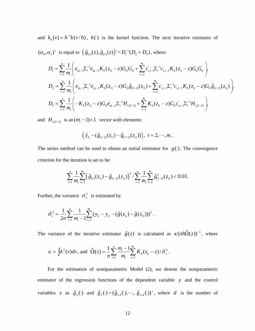
and 1( ) ( / )hk v h k v h−= , ( )k ⋅ is the kernel function. The next iterative estimator of

0 1( , ) 'α α is equal to ( )[ ] [ ]ˆ ˆ( ), ( ) 'l lg z g z = 11 2 3( )D D D− + , where:

' 1 ' ' 1 '1 1 1 1 1 1 , 1 , 1

1 2

' 1 ' 12 1 1 1 1 [ 1] 1 , 1 , 1 [ 1]

1 2

3

1 ( ) ( ) ,

1 ˆ ˆ( ) ( ) ( ) ( ) ,

1

i

i i

i

i i

mn

m i m h i i i i t i i t h it it iti ti

mn

m i m h i i l i i t i i t h it it l iti ti

i

D e e K z z G G c c K z z G Gm

D e e K z z G g z c c K z z G g zm

Dm

− −− − − −

= =

− −− − − − − −

= =

⎛ ⎞= Σ − + Σ −⎜ ⎟

⎝ ⎠⎛ ⎞

= Σ − + Σ −⎜ ⎟⎝ ⎠

=

∑ ∑

∑ ∑

' 1 ' 11 1 1 ,[ 1] , 1 ,[ 1]

1 2

( ) ( ) ,i

i

mn

h i i m i i l h it it i t i i li t

K z z G e H K z z G c H− −− − − −

= =

⎛ ⎞− − Σ + − Σ⎜ ⎟⎝ ⎠

∑ ∑

and ,[ 1]i lH − is an ( 1) 1im − × vector with elements:

( )[ 1] [ 1] 1ˆ ˆ( ( ) ( )) , 2, ,it l it l i iy g z g z t m− −− − =% L .

The series method can be used to obtain an initial estimator for ( )g ⋅ . The convergence

criterion for the iteration is set to be:

( )2 2[ ] [ 1] [ 1]

1 2 1 2

1 1ˆ ˆ ˆ( ) ( ) / ( ) 0.01.i im mn n

l it l it l iti t i ti i

g z g z g zm m− −

= = = =

− <∑ ∑ ∑ ∑

Further, the variance 2vσ is estimated by

2ˆvσ = 21 1

1 2

1 1 ˆ ˆ( ( ( ) ( )))2 1

imn

it i it ii ti

y y g z g zn m= =

− − −−∑ ∑ .

The variance of the iterative estimator ˆ ( )g z is calculated as 1ˆ( ( ))nh zκ −Ω , where

2 ( )k v dvκ = ∫ , and 2

1 2

11ˆ ˆ( ) ( ) /imn

ih it v

i ti

mz K z zn m

σ= =

−Ω = −∑ ∑ .

For the estimation of semiparametric Model (2), we denote the nonparametric

estimator of the regression functions of the dependent variable y and the control

variables x as ˆ ( )yg ⋅ and ˆ ( )xg ⋅ = ,1ˆ( ( ), ,xg ⋅ L ,ˆ ( )) 'x dg ⋅ , where d is the number of

13

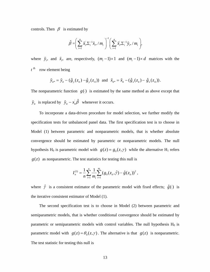
controls. Then β is estimated by

β̂ =1

' 1 ' 1* * * *

1 1/ /

n n

i i i i i i i ii i

x x m x y m−

− −

= =

⎛ ⎞ ⎛ ⎞Σ Σ⎜ ⎟ ⎜ ⎟

⎝ ⎠ ⎝ ⎠∑ ∑% % % % ,

where *iy% and *ix% are, respectively, ( 1) 1im − × and ( 1)im d− × matrices with the

t th row element being

*it ity y= −% % ˆ( ( )y itg z 1ˆ ( ))y ig z− and * ˆ( ( )it it x itx x g z= − −% % 1ˆ ( ))x ig z .

The nonparametric function ( )g ⋅ is estimated by the same method as above except that

ity% is replaced by ' ˆit ity x β−% whenever it occurs.

To incorporate a data-driven procedure for model selection, we further modify the

specification tests for unbalanced panel data. The first specification test is to choose in

Model (1) between parametric and nonparametric models, that is whether absolute

convergence should be estimated by parametric or nonparametric models. The null

hypothesis H0 is parametric model with 0( ) ( , )g z g z γ= while the alternative H1 refers

( )g z as nonparametric. The test statistics for testing this null is

(1) 20

1 1

1 1 ˆ ˆ( ( , ) ( ))imn

n it iti ti

I g z g zn m

γ= =

= −∑ ∑ ,

where γ̂ is a consistent estimator of the parametric model with fixed effects; ˆ ( )g ⋅ is

the iterative consistent estimator of Model (1).

The second specification test is to choose in Model (2) between parametric and

semiparametric models, that is whether conditional convergence should be estimated by

parametric or semiparametric models with control variables. The null hypothesis H0 is

parametric model with 0( ) ( , )g z zθ γ= . The alternative is that ( )g z is nonparametric.

The test statistic for testing this null is

14

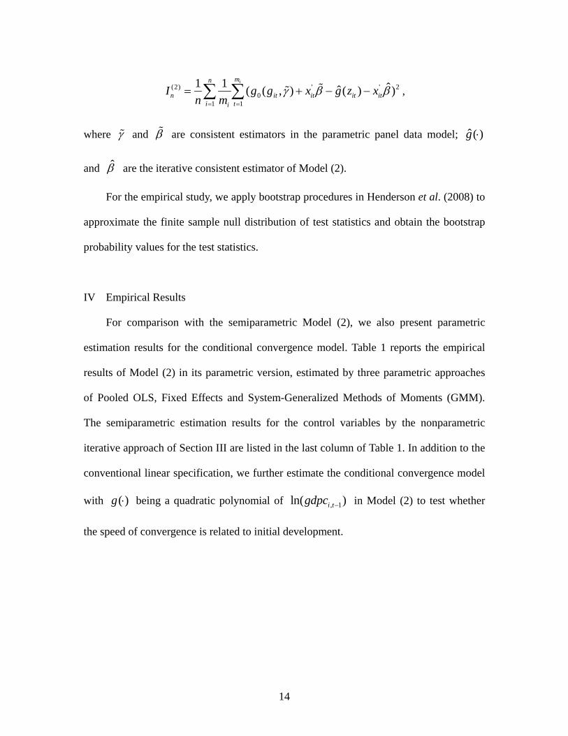
(2) ' ' 20

1 1

1 1 ˆˆ( ( , ) ( ) )imn

n it it it iti ti

I g g x g z xn m

γ β β= =

= + − −∑ ∑ %% ,

where γ% and β% are consistent estimators in the parametric panel data model; ˆ ( )g ⋅

and β̂ are the iterative consistent estimator of Model (2).

For the empirical study, we apply bootstrap procedures in Henderson et al. (2008) to

approximate the finite sample null distribution of test statistics and obtain the bootstrap

probability values for the test statistics.

IV Empirical Results

For comparison with the semiparametric Model (2), we also present parametric

estimation results for the conditional convergence model. Table 1 reports the empirical

results of Model (2) in its parametric version, estimated by three parametric approaches

of Pooled OLS, Fixed Effects and System-Generalized Methods of Moments (GMM).

The semiparametric estimation results for the control variables by the nonparametric

iterative approach of Section III are listed in the last column of Table 1. In addition to the

conventional linear specification, we further estimate the conditional convergence model

with ( )g ⋅ being a quadratic polynomial of , 1ln( )i tgdpc − in Model (2) to test whether

the speed of convergence is related to initial development.

15

Table 1 Parametric estimation results for conditional convergence models Parametric model Semiparametric

model Pooled OLS Fixed effects System-GMM gdpc -0.0126* 0.0091 -0.0704* -0.1525* -0.0251** -0.0026 ---

(0.0025) (0.0174) (0.0073) (0.0504) (0.0114) (0.0664) --- gdpc2 --- -0.0012 --- 0.0048*** --- -0.0011 ---

--- (0.0010) --- (0.0028) --- (0.0038) --- Ki 0.0185*** 0.0181*** 0.0174 0.0183 0.0459** 0.0436** 0.0259*

(0.0104) (0.0105) (0.0231) (0.0230) (0.0184) (0.0202) (0.0064) Kg -0.0105* -0.0106* -0.0421* -0.0402* -0.0226** -0.0174*** -0.0421*

(0.0025) (0.0025) (0.0092) (0.0094) (0.0103) (0.0095) (0.0049) urban -0.0009 -0.0013 -0.0014 -0.0024 -0.0083 -0.0003 -0.0052

(0.0031) (0.0031) (0.0111) (0.0113) (0.0134) (0.0146) (0.0073) co2 0.0048* 0.0047* 0.0176* 0.0188* 0.0043 0.0050 0.0331*

(0.0016) (0.0016) (0.0048) (0.0050) (0.0047) (0.0066) (0.0034) deflator -0.0185* -0.0187* -0.0224* -0.0225* -0.0182* -0.0189* -0.0216*

(0.0029) (0.0029) (0.0039) (0.0039) (0.0055) (0.0054) (0.0022) trade 0.0032 0.0028 0.0328* 0.0325* 0.0159** 0.0151 0.0299*

(0.0020) (0.0020) (0.0072) (0.0072) (0.0078) (0.0100) (0.0044) life 0.0525* 0.0500* 0.0069 0.0082 0.0818*** 0.0544 0.0303***

(0.0129) (0.0128) (0.0243) (0.0242) (0.0439) (0.0421) (0.0162) credit -0.0047** -0.0045** -0.0016 -0.0024 -0.0090 -0.0096 -0.0079*

(0.0019) (0.0019) (0.0040) (0.0039) (0.0055) (0.0059) (0.0026) Fdi 0.0357*** 0.0373*** 0.0282 0.0260 0.0666*** 0.0600 0.0011

(0.0197) (0.0200) (0.0245) (0.0239) (0.0388) (0.0402) (0.0107) Notes: The dependent variable is , 1ln( ) ln( )it i tgdpc gdpc −− . The numbers in the parentheses except in the last column are standard errors of the coefficient estimates. The numbers in the parentheses in the last column are bootstrapping standard errors. Estimates of the intercepts in parametric models are not reported. *, ** and *** indicate significance at 1%, 5%, and 10% levels, respectively. λ is the implied rate of convergence, which is calculated by (3) in the models with a linear function of gdpc and as ln( ( ) 1)gdp barβ −− + in the models with a quadratic function of gdpc, gdp bar− is the sample average of log(gdpc). The two system-GMM estimations are two-step robust. Second order correlation statistics and difference-Sargen p-values of the two system-GMM estimation show valid use of instrumental variables.

The performance of system-GMM estimator can be evaluated by establishing a

bound for the autoregressive parameter. The OLS estimator and the within-groups (fixed

effects) estimator are used to establish an upper and a lower bound, respectively, for the

estimated coefficient of the initial income term. This would mean that a consistent

16

estimate of the initial income term coefficient can be expected to lie in between the OLS

levels and within-groups estimates (Bond et al., 2001). The results shown in Table 1

support the system-GMM estimation, with the two estimates lying within those in the

OLS upper and within-groups lower bound.

The conventional linear specification of the conditional convergence model

estimated by system-GMM estimation (column 5) shows a significant negative

coefficient on the initial income term (-0.0251), while the quadratic specification (column

6) gives an insignificant coefficient estimation. The more reliable linear conditional

convergence model gives an average convergence rate of 2.5 percent (column 5) with

positive estimates on coefficients of the five control variables (investment, carbon

dioxide, trade openness, life expectancy and foreign direct investment), reflecting

differences in the steady-state equilibrium. In particular, life expectancy (8.18%) has the

greatest positive and significant effect. This agrees with the empirical evidence that

health plays an important role in determining economic growth rates (Bloom and

Canning, 2000; Bloom et al., 2001). Other variables carry different levels of impact to

economic growth – ranging from foreign direct investment (6.66%), investment share

(4.59%), trade openness (1.59%), and to carbon dioxide emission (0.43%).

On the contrary, government consumption, urbanization, inflation and private credit

share produce a negative impact to economic growth. The significant negative figures for

government size (-0.0226) and inflation (-0.0182) support the fact that inefficient

government expenditure and high inflation rates would hinder economic growth (Iradian,

2003, 2005; Fischer, 1993; Barro, 1995). On the whole, the linear specification of the

conditional convergence model estimated by the system-GMM method gives positive

estimates on investment, carbon dioxide emission, trade, life expectancy and foreign

17

direct investment, but negative values for other economic growth determinants

(government size, urbanization, inflation, and private credit share).

In our nonparametric and semiparametric estimation of Model (1) and Model (2),

the kernel is the Gaussian function and the bandwidth is chosen according to the rule of

thumb: 1/ 51.06 ( )h stdc z N −= × × , where ( )stdc z is the standard deviation of z , the

logarithm of the initial GDP per capita in the sample and N is the sample size. Both the

standard errors for the coefficient estimates in the parametric part of Model (2) and the

lower and upper bounds of 95 percent confidence intervals of the estimate ˆ ( )g ⋅ in the

nonparametric part of Model (2) are calculated by the bootstrap approach. The model

specification test statistics and the probability values for the tests are calculated by the

approach proposed in Henderson et al. (2008). All the bootstrap replications are set to be

400.

Column 7 in Table 1 shows that the coefficients estimates of the control variables in

the semiparametric conditional convergence Model (2) are identical in direction to those

in the parametric model estimated by system-GMM (in columns 5 and 6). Investment,

carbon dioxide emission, trade, life expectancy and foreign direct investment contribute

positively to economic growth while government size, urbanization, inflation, and private

credit share exert negative effects.

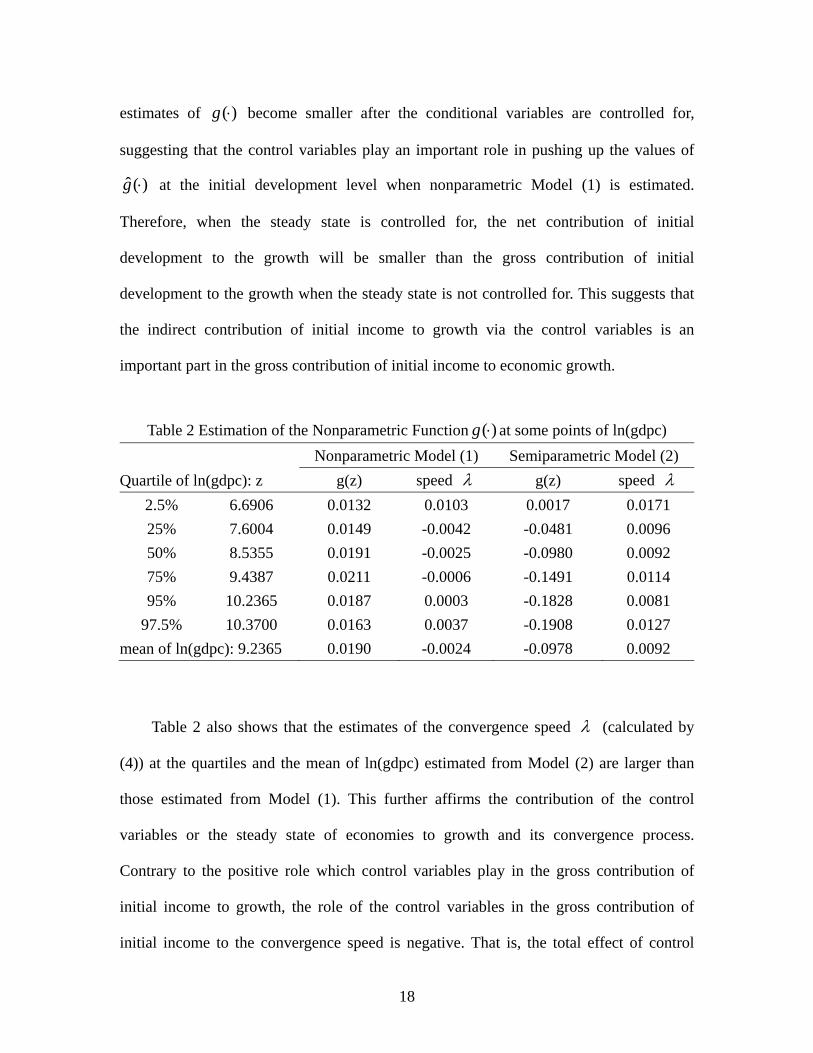
Table 2 shows the estimation of the nonparametric function and the implied speed of

convergence at some quartile points of the logarithm of initial real GDP per capita by

using both nonparametric Model (1) and semiparametric Model (2). It can be seen that

the estimates of ( )g ⋅ from semiparametric Model (2) are smaller than those from

nonparametric Model (1) at all the quartile points of ln(gdpc). This shows that the

18

estimates of ( )g ⋅ become smaller after the conditional variables are controlled for,

suggesting that the control variables play an important role in pushing up the values of

ˆ ( )g ⋅ at the initial development level when nonparametric Model (1) is estimated.

Therefore, when the steady state is controlled for, the net contribution of initial

development to the growth will be smaller than the gross contribution of initial

development to the growth when the steady state is not controlled for. This suggests that

the indirect contribution of initial income to growth via the control variables is an

important part in the gross contribution of initial income to economic growth.

Table 2 Estimation of the Nonparametric Function ( )g ⋅ at some points of ln(gdpc)

Quartile of ln(gdpc): z Nonparametric Model (1) Semiparametric Model (2)

g(z) speed λ g(z) speed λ 2.5% 6.6906 0.0132 0.0103 0.0017 0.0171 25% 7.6004 0.0149 -0.0042 -0.0481 0.0096 50% 8.5355 0.0191 -0.0025 -0.0980 0.0092 75% 9.4387 0.0211 -0.0006 -0.1491 0.0114 95% 10.2365 0.0187 0.0003 -0.1828 0.0081

97.5% 10.3700 0.0163 0.0037 -0.1908 0.0127 mean of ln(gdpc): 9.2365 0.0190 -0.0024 -0.0978 0.0092

Table 2 also shows that the estimates of the convergence speed λ (calculated by

(4)) at the quartiles and the mean of ln(gdpc) estimated from Model (2) are larger than

those estimated from Model (1). This further affirms the contribution of the control

variables or the steady state of economies to growth and its convergence process.

Contrary to the positive role which control variables play in the gross contribution of

initial income to growth, the role of the control variables in the gross contribution of

initial income to the convergence speed is negative. That is, the total effect of control

19

variables on growth is positive whereas the total effect of control variables on

convergence speed is negative.

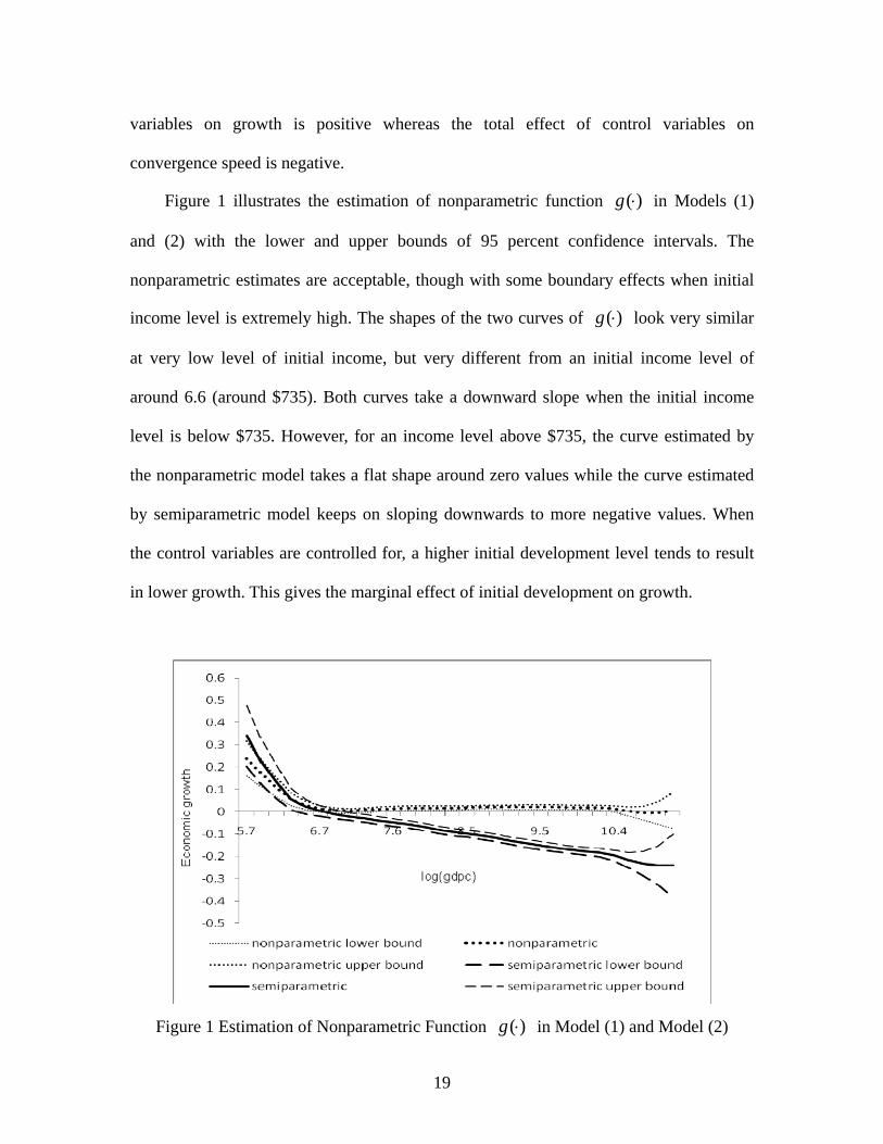
Figure 1 illustrates the estimation of nonparametric function ( )g ⋅ in Models (1)

and (2) with the lower and upper bounds of 95 percent confidence intervals. The

nonparametric estimates are acceptable, though with some boundary effects when initial

income level is extremely high. The shapes of the two curves of ( )g ⋅ look very similar

at very low level of initial income, but very different from an initial income level of

around 6.6 (around $735). Both curves take a downward slope when the initial income

level is below $735. However, for an income level above $735, the curve estimated by

the nonparametric model takes a flat shape around zero values while the curve estimated

by semiparametric model keeps on sloping downwards to more negative values. When

the control variables are controlled for, a higher initial development level tends to result

in lower growth. This gives the marginal effect of initial development on growth.

Figure 1 Estimation of Nonparametric Function ( )g ⋅ in Model (1) and Model (2)

20

Our finding is consistent with the neoclassical prediction that poor countries would

grow faster than rich countries if the only difference is their initial levels of capital (Swan,

1956). The higher the income level is, the larger the role played by the control variables

in changing the nonlinear shape of ( )g ⋅ . Since the growth is calculated by statistics in

which the effects of control variables are contained, it is mainly related to our

nonparametric estimation of ( )g ⋅ in Model (1). Therefore, our finding is also consistent

with the reality of growth, especially in developed economies, in the long run that growth

in developed countries would generally be low or close to zero. Figure 1 provides an

adaptive description on this prediction.

Figure 1 can be stated in a different way. The contribution by the steady state or

control variables to economic growth can be seen from the vertical distance between the

two curves estimated by nonparametric and semiparametric models. At income levels

below $735, the vertical distance decreases as income levels increases. The opposite

occurs for income levels above $735 – the vertical distance increases as income level

increases. The vertical distance can be explained as the channel effect of initial

development on economic growth via the control variables. Whenever the estimates of

( )g ⋅ by semiparametric model are larger than those by nonparametric model, the

channel effect is negative, but becomes positive when the opposite occurs. The control

variables as a whole cannot contribute to economic growth explained by the initial

development at or below the low income level of around $735. In some sense, they have

a dampening effect on ( )g ⋅ .

On the other hand, when the income level is above $735, the indirect or channel

effect becomes positive. This implies that the control variables as a channel tend to

21

increase economic growth at higher stage of income level. This evidence shows that

whether the control variables will have positive contribution to economic growth

explained by initial development level depends on the income levels of economies. Our

finding shows that control variables have played a negative channel effect in the growth

convergence for poor economies while they played a positive channel effect in the

convergence for developed economies. Figure 1 suggests that the absolute convergence

hypothesis tends to hold only for the economies with low per capita GDP levels (<$735).

However, the conditional convergence hypothesis tends to hold for all the economies.

Figure 2 gives a comparison of the implied speeds of convergence calculated from

the nonparametric and semiparametric regression models. Since the control variables are

used as proxies for the steady state for conditional convergence, the speed of conditional

convergence calculated from the semiparametric estimation of Model (2) has controlled

for the effects from the steady state. However, the nonparametric Model (1) has

suppressed the contribution of the control variables in the gross effect of initial income on

growth for the unconditional convergence, and hence the speed of absolute convergence

calculated from the nonparametric estimation of Model (1) has embodied the effect from

the steady state. One can see from Figure 2 that the conditional speed of convergence is

larger than the absolute counterpart at all levels of initial income. This shows that the

inclusion of the control variables in the model decreases the calculated values of the

convergence speed. This finding is essentially identical to that from Table 2. The role of

the control variables in the gross contribution of initial income to the convergence speed

is negative.

22

Figure 2 Comparing the convergence speeds calculated from Models (1) and (2)

Figure 2 also shows that both absolute and conditional convergence speeds are

decreasing with the initial development for income levels less than around 6.6 ($735)

with a steep negative slope of an average rate of around 7.3 percent. As the income levels

get higher, the two convergence rates drop. The conditional convergence speed keeps at a

steady rate of around 1.2 percent while the absolute convergence speed keeps at a rate

close to zero until a very high income level of around 10.2 ($26,903) is reached. Such a

high income level raises the absolute convergence speed to a local maximum of 1.5

percent and the conditional convergence speed to a local maximum of 2.1 percent. After

the local maximum speeds, however, the high portion of income levels show a further

decreasing trend for both convergence speeds. Figure 2 confirms the results from Figure

1: the absolute convergence hypothesis tends to hold only for the economies with low per

capita GDP levels with the speed ranging from 0.15 percent to 9 percent and tends not to

hold for most of the economies with per capita GDP greater than $735, whereas the

23

conditional convergence hypothesis holds for almost all the economies with the speed

ranging from 0.15 percent to 14 percent. The economies tend to converge more quickly to

their own steady state than to their common one.

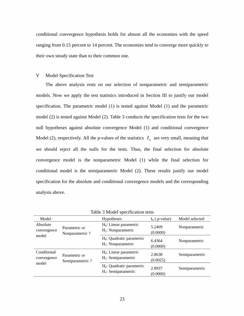
V Model Specification Test

The above analysis rests on our selection of nonparametric and semiparametric

models. Now we apply the test statistics introduced in Section III to justify our model

specification. The parametric model (1) is tested against Model (1) and the parametric

model (2) is tested against Model (2). Table 3 conducts the specification tests for the two

null hypotheses against absolute convergence Model (1) and conditional convergence

Model (2), respectively. All the p-values of the statistics nI are very small, meaning that

we should reject all the nulls for the tests. Thus, the final selection for absolute

convergence model is the nonparametric Model (1) while the final selection for

conditional model is the semiparametric Model (2). These results justify our model

specification for the absolute and conditional convergence models and the corresponding

analysis above.

Table 3 Model specification tests Model Hypotheses In ( p-value) Model selected

Absolute convergence model

Parametric or Nonparametric ?

H0: Linear parametric H1: Nonparametric

5.2409 (0.0000)

Nonparametric

H0: Quadratic parametric H1: Nonparametric

6.4364 (0.0000)

Nonparametric

Conditional convergence model

Parametric or Semiparametric ?

H0: Linear parametric H1: Semiparametric

2.8638 (0.0025)

Semiparametric

H0: Quadratic parametric H1: Semiparametric

2.8937 (0.0000)

Semiparametric

24

VI Conclusion

The multiple steady states in the cross-country growth for the world economy

confirm that there is nonlinearity and non-constant implied rates of convergence between

different groups of economies in the convergence process. This article investigates the

absolute and conditional convergence of real GDP per capita among 164 world

economies over the period 1970-2006 by using the estimation of nonparametric and

semiparametric unbalanced panel data models with fixed effects.

Our econometric estimations on growth convergence can be evaluated with

reference to a number of parametric empirical studies that have chosen similar variables

in their analysis of the conditional convergence issue. However, the data-driven model

specification tests justify the use of nonparametric and semiparametric models to study

absolute and conditional convergence processes instead of the conventional parametric

counterparts. The semiparametric results show that the proxy variables of the steady state

such as investment, carbon dioxide emission, trade, life expectancy and foreign direct

investment contribute positively to economic growth while the other determinants such as

government size, urbanization, inflation, and private credit share exert negative effects.

The comparison between nonparametric and semiparametric results shows that the

indirect contribution of initial income to growth via the control variables is an important

part in the gross contribution of initial income to economic growth. The total effect of

control variables on growth is positive whereas the total effect on the convergence speed

is negative. Control variables play a negative channel effect in the growth convergence

for poor economies, but a positive channel effect in the convergence for developed

economies. The absolute convergence hypothesis tends to hold only for the economies

25

with low per capita GDP levels (<$735). However, the conditional convergence

hypothesis tends to hold for all the economies.

Both absolute and conditional convergence speeds are decreasing with the initial

development for income levels less than around 6.6 ($735) with a steep negative slope of

an average rate of around 7.3 percent. The conditional convergence speed keeps at a

steady rate of around 1.2 percent while the absolute convergence speed keeps at a rate

close to zero until a very high income level of around 10.2 ($26,903) is reached. The

economies tend to converge more quickly to their own steady state than to their common

one. The absolute convergence hypothesis tends to hold only for the economies with low

per capita GDP levels with the speed ranging from 0.15 percent to 9 percent and tends

not to hold for most of the economies with per capita GDP greater than $735, whereas the

conditional convergence hypothesis holds for almost all the economies with the speed

ranging from 0.15 percent to 14 percent.

26

References Annez, P. C., and Buckley, R. M., (2009), “Urbanization and growth: setting the context”, In Spence, M., Annez, P.C., and Buckey, R. M. (Eds.), Urbanization and Growth, IBRD, Washington D. C.: The World Bank. Azomahou, T., J. E. Ouardighi, P. Nguyen-Van, and T. K. C. Pham (2011), “Testing

convergence of European regions: a semiparametric approach”, Economic Modelling 28: 1202-1210.

Barro, R. J., (1995), Inflation and Economic Growth, NBER Working Paper Series, Working Paper 5326. Barro, R. J. and Sala-i-Martin, X., (1990), “Convergence across states and regions”, Brooking Papers on Economic Activities, 1, 107-182. Barro, R. J. and Sala-i-Martin, X., (1992), “Convergence”, Journal of Political Economy, 100(2), 223-251. Baumol, W. J., (1986), “Productivity, growth, convergence and welfare: what the long-run data show”, American Economic Review, 76(5), 1972-1885. Bianchi, M., (1997), “Testing for convergence: evidence from non-parametric multimodality tests”, Journal of Applied Econometrics, 12, 393-409 Bond, S., Hoeffler, A., and Temple, J., (2001), GMM Estimation of Empirical Growth Models, CERP Discussion Paper No. 3048. Bloom, D., and Canning, D., (2000), “The health and wealth of nations”, Science, 287, 1207-1209. Bloom, D., Canning, D., and Sevilla, J., (2001), The Effect of Health on Economic Growth: Theory and Evidence, NBER, Working Paper 8587. Dobson, S., C. Ramlogan and E. Strobl (2003), “Cross-country growth and convergence:

a semiparametric analysis”, Economics Discussion Papers No. 0301, University of Otago, ISSN 0111-1760.

Dollar, D. and Kraay, A., (2001), “Trade, growth and poverty”, Economic Journal, 114 (February), 22-49. Duranton, G., (2009), “Are cities engines of growth and prosperity for developing countries?”, In Spence, M., Annez, P. C., and Buckey, R. M. (Eds), Urbanization and Growth, IBRD, Washington D. C.: The World Bank. Evans, P., and Kim, J. U., (2005), “Estimating convergence for Asian economies using dynamic random variable models”, Economic Letters, 86, 159-166. Frankel, J. A., and Romer, D., (1999), “Does trade cause growth?” American Economic Review, 89, 379-399. Henderson D. J., Corroll, R. J., and Li, Q., (2008), “Nonparametric estimation and testing

27

of fixed effects panel data models”, Journal of Econometrics, 144: 257-275. Im, K., Pesaran, M., and Shin, Y., (1997), Testing for Unit Roots in Heterogenous Panels, DAE Working Paper Amalgamated Series No. 9526, University of Cambridge. Iradian, G., (2003), Armenia: The Road to Sustained Rapid Growth, Cross-country Evidence, IMF Working Paper 02/103, Washington D. C.: International Monetary Fund. Iradian, G., (2005), Inequality, Poverty, and Growth: Cross-country Evidence, IMF Working Paper 05/28, Washington D. C.: International Monetary Fund. Islam, N., (1995), “Growth empirics: a panel data approach”, Quarterly Journal of

Economics, 109, 1127-1170. Islam, N., (2003), “What have we learnt from the convergence debate?”, Journal of

Economic Survey, 17, 309-362. Juessen, F., (2009), “A distribution dynamics approach to regional GDP convergence in unified Germany”, Empirical Economics, 37, 627-652. Kumer, S. and A. Ullah (2000), “Semiparametric varying parametric panel data models:

an application to estimation of speed of convergence”, Advances in Econometrics, Vol. 14, pp.109-128.

Levin, A., and Lin, C., (1993), Unit Root Tests in Panel Data: New Results, Economics Working Paper Series 93-56, University of California San Diego. Makki, S. S. and Somwaru, A., (2004), “Impact of foreign direct investment and trade on economic growth: evidence from developing countries”, American Journal of Agricultural Economics, 86 (3), 795-801. Quah, D., (1994), “Exploiting cross-section variations of unit root inference in dynamic data”, Economics Letters, 44, 9-19. Quah, D., (1997), “Empirics for growth and distribution: stratification, polarization, and convergence clubs”, Journal of Economic Growth, Vol. 2, 27-59. Quigley, J. M., (2009), “Urbanization, agglomeration, and economic development”, In Spence, M., Annez, P. C., and Buckey, R. M. (Eds), Urbanization and Growth, IBRD, Washington D. C.: The World Bank. Rassekh, F. (1998), “The Convergence Hypothesis: History, Theory, and Evidence”,

Open Economies Review 9: 85-105. Swan, T. W., (1956), “Economic growth and capital accumulation”, Economic Record, 32(63), 334-361. Wang, Y., (2004), “A nonparametric analysis of the personal income distribution across the provinces and states in the U.S. and Canada”, Regional and Sectoral Economic Studies, 4-1.

28

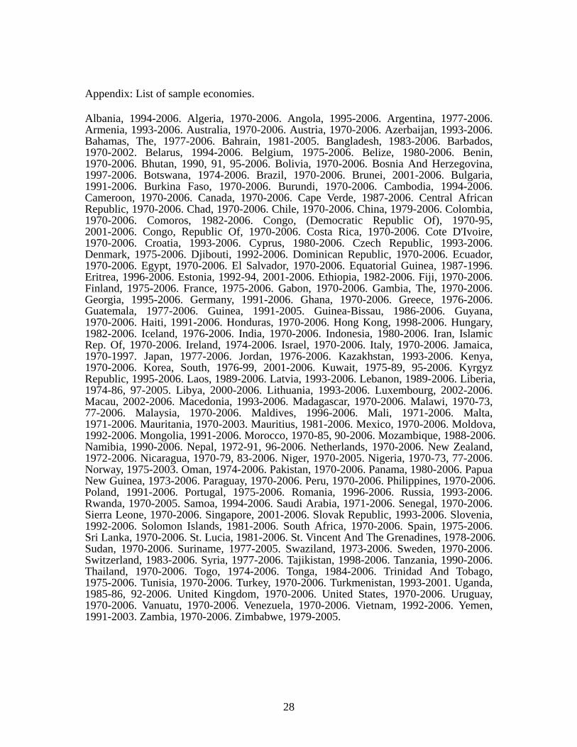
Appendix: List of sample economies. Albania, 1994-2006. Algeria, 1970-2006. Angola, 1995-2006. Argentina, 1977-2006. Armenia, 1993-2006. Australia, 1970-2006. Austria, 1970-2006. Azerbaijan, 1993-2006. Bahamas, The, 1977-2006. Bahrain, 1981-2005. Bangladesh, 1983-2006. Barbados, 1970-2002. Belarus, 1994-2006. Belgium, 1975-2006. Belize, 1980-2006. Benin, 1970-2006. Bhutan, 1990, 91, 95-2006. Bolivia, 1970-2006. Bosnia And Herzegovina, 1997-2006. Botswana, 1974-2006. Brazil, 1970-2006. Brunei, 2001-2006. Bulgaria, 1991-2006. Burkina Faso, 1970-2006. Burundi, 1970-2006. Cambodia, 1994-2006. Cameroon, 1970-2006. Canada, 1970-2006. Cape Verde, 1987-2006. Central African Republic, 1970-2006. Chad, 1970-2006. Chile, 1970-2006. China, 1979-2006. Colombia, 1970-2006. Comoros, 1982-2006. Congo, (Democratic Republic Of), 1970-95, 2001-2006. Congo, Republic Of, 1970-2006. Costa Rica, 1970-2006. Cote D'Ivoire, 1970-2006. Croatia, 1993-2006. Cyprus, 1980-2006. Czech Republic, 1993-2006. Denmark, 1975-2006. Djibouti, 1992-2006. Dominican Republic, 1970-2006. Ecuador, 1970-2006. Egypt, 1970-2006. El Salvador, 1970-2006. Equatorial Guinea, 1987-1996. Eritrea, 1996-2006. Estonia, 1992-94, 2001-2006. Ethiopia, 1982-2006. Fiji, 1970-2006. Finland, 1975-2006. France, 1975-2006. Gabon, 1970-2006. Gambia, The, 1970-2006. Georgia, 1995-2006. Germany, 1991-2006. Ghana, 1970-2006. Greece, 1976-2006. Guatemala, 1977-2006. Guinea, 1991-2005. Guinea-Bissau, 1986-2006. Guyana, 1970-2006. Haiti, 1991-2006. Honduras, 1970-2006. Hong Kong, 1998-2006. Hungary, 1982-2006. Iceland, 1976-2006. India, 1970-2006. Indonesia, 1980-2006. Iran, Islamic Rep. Of, 1970-2006. Ireland, 1974-2006. Israel, 1970-2006. Italy, 1970-2006. Jamaica, 1970-1997. Japan, 1977-2006. Jordan, 1976-2006. Kazakhstan, 1993-2006. Kenya, 1970-2006. Korea, South, 1976-99, 2001-2006. Kuwait, 1975-89, 95-2006. Kyrgyz Republic, 1995-2006. Laos, 1989-2006. Latvia, 1993-2006. Lebanon, 1989-2006. Liberia, 1974-86, 97-2005. Libya, 2000-2006. Lithuania, 1993-2006. Luxembourg, 2002-2006. Macau, 2002-2006. Macedonia, 1993-2006. Madagascar, 1970-2006. Malawi, 1970-73, 77-2006. Malaysia, 1970-2006. Maldives, 1996-2006. Mali, 1971-2006. Malta, 1971-2006. Mauritania, 1970-2003. Mauritius, 1981-2006. Mexico, 1970-2006. Moldova, 1992-2006. Mongolia, 1991-2006. Morocco, 1970-85, 90-2006. Mozambique, 1988-2006. Namibia, 1990-2006. Nepal, 1972-91, 96-2006. Netherlands, 1970-2006. New Zealand, 1972-2006. Nicaragua, 1970-79, 83-2006. Niger, 1970-2005. Nigeria, 1970-73, 77-2006. Norway, 1975-2003. Oman, 1974-2006. Pakistan, 1970-2006. Panama, 1980-2006. Papua New Guinea, 1973-2006. Paraguay, 1970-2006. Peru, 1970-2006. Philippines, 1970-2006. Poland, 1991-2006. Portugal, 1975-2006. Romania, 1996-2006. Russia, 1993-2006. Rwanda, 1970-2005. Samoa, 1994-2006. Saudi Arabia, 1971-2006. Senegal, 1970-2006. Sierra Leone, 1970-2006. Singapore, 2001-2006. Slovak Republic, 1993-2006. Slovenia, 1992-2006. Solomon Islands, 1981-2006. South Africa, 1970-2006. Spain, 1975-2006. Sri Lanka, 1970-2006. St. Lucia, 1981-2006. St. Vincent And The Grenadines, 1978-2006. Sudan, 1970-2006. Suriname, 1977-2005. Swaziland, 1973-2006. Sweden, 1970-2006. Switzerland, 1983-2006. Syria, 1977-2006. Tajikistan, 1998-2006. Tanzania, 1990-2006. Thailand, 1970-2006. Togo, 1974-2006. Tonga, 1984-2006. Trinidad And Tobago, 1975-2006. Tunisia, 1970-2006. Turkey, 1970-2006. Turkmenistan, 1993-2001. Uganda, 1985-86, 92-2006. United Kingdom, 1970-2006. United States, 1970-2006. Uruguay, 1970-2006. Vanuatu, 1970-2006. Venezuela, 1970-2006. Vietnam, 1992-2006. Yemen, 1991-2003. Zambia, 1970-2006. Zimbabwe, 1979-2005.