Cross-correlation of the cosmic microwave background with the 2MASS galaxy survey: Signatures of dark energy, hot gas, and point sources

arX

iv:a

stro

-ph/

0308

260v

4 3

Feb

200

4v2.1, astro-ph/0308260

February 2, 2008

Cross-Correlation of the Cosmic Microwave Background with the

2MASS Galaxy Survey:

Signatures of Dark Energy, Hot Gas, and Point Sources

Niayesh Afshordi,∗ Yeong-Shang Loh, and Michael A. Strauss

Princeton University Observatory, Princeton, NJ 08544, USA

Abstract

We cross-correlate the Cosmic Microwave Background (CMB) temperature anisotropies observed

by the Wilkinson Microwave Anisotropy Probe (WMAP) with the projected distribution of ex-

tended sources in the Two Micron All Sky Survey (2MASS). By modelling the theoretical expecta-

tion for this signal, we extract the signatures of dark energy (Integrated Sachs-Wolfe effect;ISW),

hot gas (thermal Sunyaev-Zeldovich effect;thermal SZ), and microwave point sources in the cross-

correlation. Our strongest signal is the thermal SZ, at the 3.1−3.7σ level, which is consistent with

the theoretical prediction based on observations of X-ray clusters. We also see the ISW signal at

the 2.5σ level, which is consistent with the expected value for the concordance ΛCDM cosmology,

and is an independent signature of the presence of dark energy in the universe. Finally, we see the

signature of microwave point sources at the 2.7σ level.

PACS numbers: 98.65., 98.65.Dx, 98.65.Hb, 98.70.Dk, 98.70.Vc, 98.80., 98.80.Es

∗Electronic address: [email protected]

1

I. INTRODUCTION

The recently released WMAP [5] results constrain our cosmology with an unprecedented

accuracy. Most of these constraints come from the linear fossils of the early universe which

have been preserved in the temperature anisotropies of the CMB. These are the ones that can

be easily understood and dealt with, within the framework of linear perturbation theory.

However, there are also imprints of the late universe which could be seen in the WMAP

results. Most notably, the measurement of the optical depth to the surface of last scattering,

τ ≃ 0.17, which implied an early reionization of the universe, was the biggest surprise. There

is also the strangely small amplitude of the large-angle CMB anisotropies which remains

unexplained[49].

Can we extract more about the late universe from WMAP? Various secondary effects

have been studied in the literature (see e.g.[23] which lists a few). The main secondary

anisotropy at large angles is the so-called Integrated Sachs-Wolfe (ISW) effect[43], which is

a signature of the decay of the gravitational potential at large scales. This could be either a

result of spatial curvature, or presence of a component with negative pressure, the so-called

dark energy, in the universe[40]. Since WMAP has constrained the deviation from flatness

to less than 4%, the ISW effect may be interpreted as a signature of dark energy. At smaller

angles, the dominant source of secondary anisotropy is the thermal Sunyaev-Zeldovich (SZ)

effect[54], which is due to scattering of CMB photons by hot gas in the universe.

However, none of these effects can make a significant contribution to the CMB power

spectrum below ℓ ∼ 1000, and thus they are undetectable by WMAP alone. One pos-

sible avenue is cross-correlating CMB anisotropies with a tracer of the density in the late

universe[11, 13, 41]. This was first done by [8] who cross-correlated the COBE/DMR map[4]

with the NRAO VLA Sky Survey (NVSS)[10]. After the release of WMAP, different groups

cross-correlated the WMAP temperature maps with various tracers of the low-redshift uni-

verse. This was first done with the ROSAT X-ray map in [14], where a non-detection of the

thermal SZ effect puts a constraint on the hot gas content of the universe. [20] claimed a

2-5σ detection of an SZ signal by filtering WMAP maps via templates made using known

X-ray cluster catalogs. [38] looked at the cross-correlation with the NVSS radio galaxy sur-

vey, while [9] repeated the exercise for NVSS, as well as the HEAO-1 hard X-ray background

survey, both of which trace the universe around redshift of ∼ 1. Both groups found their

2

result to be consistent with the expected ISW signal for the WMAP concordance cosmology

[5], i.e. a flat ΛCDM universe with Ωm ≃ 0.3, at the 2 − 3σ level. Their result is consistent

with the ΛCDM paradigm which puts most of the energy of the universe in dark energy[40].

More recently, [16] cross-correlated WMAP with the APM galaxy survey[34] which traces

the galaxy distribution at z ∼ 0.15. This led to an apparent detection of both the thermal

SZ and ISW signals. However, the fact that they use a jack-knife covariance matrix to

estimate the strength of their signal, while their jack-knife errors are significantly smaller

than those obtained by Monte-Carlo realizations of the CMB sky (compare their Figure

2 and Figure 3) weakens the significance of their claim. Indeed, as we argue below (see

III.C), using Monte-Carlo realizations of the CMB sky is the only reliable way to estimate

a covariance matrix if the survey does not cover the whole sky.

[36] cross-correlates the highest frequency band (W-band) of the WMAP with the ACO

cluster survey[1], as well as the galaxy groups and clusters in the APM galaxy survey.

They claim a 2.6σ detection of temperature decrement on angles less than 0.5, which they

associate with the thermal SZ effect. However they only consider the Poisson noise in their

cluster distribution as their source of error. This underestimates the error due to large spatial

correlations (or cosmic variance) in the cluster distribution (see III.C). [36] also studies the

cross-correlation of the W-band with the NVSS radio sources below a degree and claims

a positive correlation at the scale of the W-band resolution. This may imply a possible

contamination of the ISW signal detection in [9] and [38]. However the achromatic nature

of this correlation makes this unlikely[7].

Finally, [46] and [17] repeated the cross-correlation analysis with the 3400 and 2000 square

degrees, respectively, of the Sloan Digital Sky Survey[52]. Both groups claim detection of a

positive signal, but they both suffer from the inconsistency of their jack-knife and Monte-

Carlo errors.

The 2MASS Extended Source Catalog (XSC)[26] is a full sky, near infrared survey of

galaxies whose median redshift is around z ∼ 0.1. The survey has reliable and uniform

photometry of about 1 million galaxies, and is complete, at the 90% level for K-magnitudes

brighter than 14, over ∼ 70% of the sky. The large area coverage and number of galaxies

makes the 2MASS XSC a good tracer of the ISW and SZ signals in the cross-correlation

with the CMB.

In this paper, we study the cross-correlation of the WMAP Q,V and W bands

3

with four different K-magnitude bins of the 2MASS Extended Source Catalog, and

fit it with a three component model which includes the ISW, thermal SZ effects and

microwave sources. We compare our findings with the theoretical expectations from

the WMAP+CBI+ACBAR+2dF+Ly-α best fit cosmological model (WMAP concordance

model from here on; see Table 3 in [5]), which is a flat universe with, Ωm = 0.27, Ωb =

0.044, h = 0.71, and σ8 = 0.84. We also assume their values of ns = 0.93, and

dns/d ln k = −0.031 for the spectral index and its running at k = 0.05 Mpc [49].

We briefly describe the relevant secondary anisotropies of the CMB in Sec. II. Sec. III

describes the properties of the cross-correlation of two random fields, projected on the sky.

Sec. IV summarizes the relevant information on the WMAP temperature maps and the

2MASS Extended Source Catalog. Sec. V describes our results and possible systematics,

and Sec. VI concludes the paper.

II. WHAT ARE THE SECONDARY ANISOTROPIES?

The dominant nature of the Cosmic Microwave Background (CMB) fluctuations, at angles

larger than ∼ 0.1 degree, is primordial, which makes CMB a snapshot of the universe at

radiation-matter decoupling, around redshift of ∼ 1000. However, a small part of these

fluctuations can be generated as the photons travel through the low redshift universe. These

are the so-called secondary anisotropies. In this section, we go through the three effects which

should dominate the WMAP/2MASS cross-correlation.

A. Integrated Sachs-Wolfe effect

The first one is the Integrated Sachs-Wolfe (ISW) effect[43] which is caused by the time

variation in the cosmic gravitational potential, Φ. For a flat universe, the anisotropy due to

the ISW effect is an integral over the conformal time η

δISW(n) = 2

∫

Φ′

[(η0 − η)n, η] dη, (1)

where Φ′

≡ ∂Φ/∂η, and n is unit vector in the line of sight. The linear metric is assumed

to be

ds2 = a2(η)[1 + 2Φ(x, η)]dη2 − [1 − 2Φ(x, η)]dx · dx, (2)

4

and η0 is the conformal time at the present.

In a flat universe, the gravitational potential Φ is constant for a fixed equation of state

and therefore observation of an ISW effect is an indicator of a change in the equation of

state of the universe. Assuming that this change is due to an extra component in the matter

content of the universe, the so-called dark energy, this component should have a negative

pressure to become important at late times[40]. Therefore, observation of an ISW effect in

a flat universe is a signature of dark energy.

The ISW effect is observed at large angular scales because most of the power in the

fluctuations of Φ is at large scales. Additionally, the fluctuations at small angles tend to

cancel out due to the integration over the line of sight.

B. Thermal Sunyaev-Zeldovich effect

The other significant source of secondary anisotropies is the so-called thermal Sunyaev-

Zeldovich (SZ) effect [54], which is caused by the scattering of CMB photons off the hot

electrons of the intra-cluster medium. This secondary anisotropy is frequency dependent,

i.e. it cannot be associated with a single change in temperature. If we define a frequency

dependent T (ν) so that IB[ν; T (ν)] = I(ν), where I(ν) is the CMB intensity and IB[ν; T ] is

the black-body spectrum at temperature T , the SZ anisotropy takes the form

δT (ν)

T (ν)= −

σT f(x)

mec

∫

δpe[(η0 − η)n, η]a(η) dη, (3)

where

x ≡ hν/(kBTCMB

) and f(x) ≡ 4 − x coth(x/2), (4)

and pe is the electron pressure. Assuming a linear pressure bias with respect to the matter

overdensity δm:

δpe

pe

= bpδm, (5)

Eq.(3) can be written as

δSZ(ν) ≡δT (ν)

T (ν)= −F (x)

∫

TeδmH0dη

a2(η), (6)

where

Te = bpTe,

F (x) = nekBσT f(x)4mecH0

= (1.16 × 10−4keV−1)Ωbhf(x), (7)

5

and Te and ne are the average temperature and the comoving density of (all) electrons,

respectively. In Appendix A, we make an analytic estimate for Te, based on the mass

function and mass-temperature relation of galaxy clusters.

C. Microwave Sources

Although technically they are not secondary anisotropies, microwave sources may con-

tribute to the cross-correlation signal, as they are potentially observable by both WMAP

and 2MASS. For simplicity, we associate an average microwave luminosity with all 2MASS

sources. We can relax this assumption by taking this luminosity to be a free parameter for

each magnitude bin, and/or removing the clustering of the point sources. As we discuss in

Sec. V.C, neither of these change our results significantly.

For the microwave spectrum in different WMAP frequencies, we try both a steeply falling

antenna temperature ∝ 1/ν2−3 (consistent with WMAP point sources[6]) and a Milky Way

type spectrum which we obtain from the WMAP observations of the Galactic foreground

[6].

In Appendix B, assuming an exponential surface emissivity with a scale length of 5 kpc

for the Galactic disk and a small disk thickness, we use the Galactic latitude dependence of

the WMAP temperature to determine the luminosity of the Milky Way (Eq.B6) in different

WMAP bands:

L∗

Q = 1.7 × 1037 erg s−1,

L∗

V = 3.0 × 1037 erg s−1,

and L∗

W = 1.0 × 1038 erg s−1. (B6)

These values are within 50% of the observed WMAP luminosity of the Andromeda

galaxy(see Appendix B) [55]. In V.C, we compare the observed average luminosity of the

2MASS sources to these numbers (see Table II).

The contribution to the CMB anisotropy due to Point Sources (see Eq.B2) is given by

δPS(n) =δT (n)

T=

4π2~

3c2 sinh2(x/2)L(x)

(xkBTCMB

)4∆x

∫

dr

(

r

dL(r)

)2

nc(r)δg(r, n), (8)

where ∆x is the effective bandwidth of the WMAP band[5], nc(r) is the average comov-

ing number density of the survey galaxies, dL is luminosity distance, and δg is the galaxy

overdensity.

6

III. THE CROSS-CORRELATION POWER SPECTRUM

A. The Expected Signal

We first develop the theoretical expectation value of the cross-correlation of two random

fields, projected on the sky. Let us consider two random fields A(x) and B(x) with their

Fourier transforms defined as

Ak =

∫

d3x e−ik.xA(x), and Bk =

∫

d3x e−ik.xB(x). (9)

The cross-correlation power spectrum, PAB(k) is defined by

〈Ak1Bk2

〉 = (2π)3δ3(k1 − k2)PAB(k1). (10)

The projections of A and B on the sky are defined using FA and FB projection kernels

A(n) =

∫

dr FA(r)A(rn), and B(n) =

∫

dr FB(r)B(rn). (11)

For the secondary temperature anisotropies, these kernels were given in Eqs.1,6 and 8.

For the projected galaxy overdensity, this kernel is

Fg(r) =r2 nc(r)

∫

dr′ r′2 nc(r′). (12)

For our treatment, we assume a constant galaxy bias, bg, which relates the galaxy fluctua-

tions, δg, to the overall matter density fluctuations δm, up to a shot noise δp

δg = bgδm + δp. (13)

In this work, we constrain the galaxy bias, bg, by comparing the auto-correlation of the

galaxies with the expected matter auto-correlation in our cosmological model. Our bias,

therefore, is model dependent.

Now, expanding A and B in terms of spherical harmonics, the cross-power spectrum,

CAB(ℓ) is defined as

CAB(ℓ) ≡ 〈AℓmB∗

ℓm〉

=∫

dr1dr2FA(r1)FB(r2)×∫

d3k

(2π)3PAB(k)(4π)2jℓ(kr1)jℓ(kr2)Yℓm(k)Y ∗

ℓm(k)

=∫

dr1dr2FA(r1)FB(r2)∫

2k2dkπ

jℓ(kr1)jℓ(kr2)PAB(k),

(14)

7

where jℓ’s are the spherical Bessel functions of rank ℓ and Yℓm’s are the spherical harmonics.

To proceed further, we use the small angle (large ℓ) approximation for the spherical Bessel

functions

jℓ(x) =

√

π

2ℓ + 1[δDirac(ℓ +

1

2− x) + O(ℓ−2)], (15)

which yields

CAB(ℓ) =

∫

dr

r2FA(r)FB(r)PAB

(

ℓ + 1/2

r

)

· [1 + O(ℓ−2)]. (16)

This is the so called Limber equation [33]. As we do not use the quadrupole due to its

large Galactic contamination, the smallest value of ℓ that we use is 3. Direct integration

of Eq.(15) (for the ISW signal which is dominant for low ℓ’s, see Figure 7) shows that the

Limber equation overestimates the cross-power by less than 2-3% at ℓ = 3, which is negligible

compared to the minimum cosmic variance error (about 40%, see III.B) at this multipole.

Therefore, the Limber equation is an accurate estimator of the theoretical power spectrum.

Now we can substitute the results of Sec. II (Eqs.1, 6, 8 and 12) into Eq.(16) which yields

CgT (x, ℓ) =bg

∫

dr r2nc(r)

∫

dr nc(r)2PΦ′,m

(

ℓ + 1/2

r

)

−

[

F (x)TeH0(1 + z)2 −4π2

~3c2 sinh2(x/2)bgL(x)

(xkBTCMB

)4∆x(1 + z)2

]

P

(

ℓ + 1/2

r

)

, (17)

where P (k) is the matter power spectrum, z is the redshift, and x is defined in Eq.(4). The

terms in Eq.(17) are the ISW, SZ and Point Source contributions respectively. Since the

ISW effect is only important at large scales, the cross-power of the gravitational potential

derivative with matter fluctuations can be expressed in terms of the matter power spectrum,

using the Poisson equation and linear perturbation theory, and thus we end up with

CgT (x, ℓ) =bg

∫

dr r2nc(r)

∫

dr nc(r)−3H20Ωm

r2

(ℓ + 1/2)2·g′

g(1 + z)

−F (x)Te(1 + z)2 +4π2

~3c2 sinh2(x/2)bgL(x)

(xkBTCMB

)4∆x(1 + z)2P

(

ℓ + 1/2

r

)

, (18)

where g is the linear growth factor of the gravitational potential,Φ, and g′ is its derivative

with respect to the conformal time. We will fit this model to our data in Sec. V, allowing

a free normalization for each term.

Finally, we write the theoretical expectation for the projected galaxy auto-power,Cgg,

which we use to find the galaxy bias. Combining Eqs.12,13 and 16, we arrive at

Cgg(ℓ) =

∫

dr r2 n2c(r)[b

2g · P

(

ℓ+1/2r

)

+ γ · n−1c (r)]

[∫

dr r2 nc(r)]2 , (19)

8

where the n−1c term is the power spectrum of the Poisson noise, δp, while the extra free

parameter, γ, is introduced to include the possible corrections to the Poisson noise due to

the finite pixel size. In the absence of such corrections γ = 1. In Sec. V, we seek the values

of bg and γ that best fit our observed auto-power for each galaxy sub-sample.

To include the effects of non-linearities in the galaxy power spectrum, we use the Peacock

& Dodds fitting formula [39] for the non-linear matter power spectrum, P (k).

B. Theoretical errors: cosmic variance vs. shot noise

To estimate the expected theoretical error, again for simplicity, we restrict the calculation

to the small angle limit. In this limit, the cross-correlation function can be approximated

by

CAB(ℓ) ≃4π

∆Ω〈Aℓm B∗

ℓm〉, (20)

where ∆Ω is the common solid angle of the patch of the sky covered by observations of both

A and B[51].

Assuming gaussianity, the standard deviation in CAB, for a single harmonic mode, is

given by

∆C2AB(ℓ) = 〈C2

AB(ℓ)〉 − 〈CAB(ℓ)〉2

= ∆Ω−2[〈Aℓm B∗

ℓm〉〈Aℓm B∗

ℓm〉 + 〈Aℓm A∗

ℓm〉〈Bℓm B∗

ℓm〉]

= C2AB(ℓ) + CAA(ℓ)CBB(ℓ). (21)

The number of modes available between ℓ and ℓ + 1, in the patch ∆Ω, is

∆N ≃(2ℓ + 1)∆Ω

4π, (22)

and so the standard deviation of CAB, averaged over all these modes is

∆C2AB(ℓ) ≃

4π

∆Ω(2ℓ + 1)[C2

AB(ℓ) + CAA(ℓ)CBB(ℓ)]. (23)

In fact, since the main part of CMB fluctuations is of primordial origin, the first term

in brackets is negligible for the cross-correlation error, so the error in the cross-correlation

function, as one may expect, depends on the individual auto-correlations.

9

We can use the CMBFAST code [47] to calculate the auto-correlation of the CMB tem-

perature fluctuations. Also, the theoretical expectation for the auto-power of the projected

galaxy distribution is given by Eq.(19).

The galaxy/CMB auto-power spectra are dominated by Poisson(shot) noise/detector

noise at large ℓ’s. Therefore, the measurement of the thermal SZ signal, which becomes

important at large ℓ’s, is limited by the number of observed galaxies, as well as the resolu-

tion of the CMB detector (the angle at which signal-to-noise ratio for the CMB measurement

is of order unity). On the other hand, for the small ℓ portion of the cross-correlation which

is relevant for the ISW signal, the error is set by the matter and CMB power spectra and

thus, is only limited by cosmic variance. The only way to reduce this error is by observing a

larger volume of the universe in the redshift range 0 < z < 1, where dark energy dominates.

C. A Note On the Covariance Matrices

We saw in Section III.C that the errors in cross-correlations could be expressed in terms

of the theoretical auto-correlation. However, this is not the whole story.

We have a remarkable understanding of the auto-power spectrum of the CMB. However,

if one tries to use the frequency information to, say subtract out the microwave sources, the

simple temperature auto-power does not give the cross-frequency terms in the covariance

matrix. In fact, in the absence of a good model, the only way to constrain these terms is

by using the cross-correlation of the bands themselves. Of course, this method is limited by

cosmic variance and hence does not give an accurate result at low multipoles. To solve this

problem, we use the WMAP concordance model CMB auto-power for ℓ ≤ 13. Since there is

no frequency-dependent signal at low ℓ’s, we only use the W-band information, which has

the lowest Galactic contamination [6], for our first 4 ℓ-bins which cover 3 ≤ ℓ ≤ 13 (see the

end of Sec. III.D for more on our ℓ-space binning).

There is a similar situation for the contaminants of the 2MASS galaxy catalog. Systematic

errors in galaxy counts, due to stellar contamination or variable Galactic extinction, as

well as observational calibration errors, may introduce additional anisotropies in the galaxy

distribution which are not easy to model. Again, the easiest way to include these systematics

in the error is by using the auto-correlation of the observed galaxy distribution, which is

inaccurate for low multipoles, due to cosmic variance. Unfortunately, this is also where we

10

expect to see possible Galactic contamination or observational systematics. With this in

mind, we try to avoid this problem by excluding the quadrupole, C(2), from our analysis.

At this point, we should point out a misconception about the nature of Monte-Carlo vs.

jack-knife error estimates in some previous cross-correlation analyses, specifically [16, 17].

Many authors have used Gaussian Monte-Carlo realizations of the CMB sky to estimate

the covariance matrix of their real-space cross-correlation functions[9, 16, 17, 46]. The

justification for this method is that, since the first term in Eq.(23) is much smaller than

the second term, the error in cross-correlation for any random realization of the maps is

almost the same as the true error, and the covariance of the cross-correlation, obtained from

many random Gaussian realizations is an excellent estimator of the covariance matrix. We

may also obtain error estimates based on random realizations of one of the maps, as long

as the observed auto-power is a good approximation of the true auto-power, i.e. the cosmic

variance is low, which should be the case for angles smaller than 20 degrees (ℓ > 10). Of

course, at larger angles, as we mentioned above, one is eventually limited by the systematics

of the galaxy survey and, unless they are understood well enough, since theoretical error

estimate is not possible, there will be no better alternative rather than Monte-Carlo error

estimates. In fact, contrary to [16, 17], if anything, the presence of cross-correlation makes

Monte-Carlo errors a slight underestimate (see Eq.23). On the other hand, there is no

rigorous justification for the validity of jack-knife covariance matrices, and the fact that

jack-knife errors could be smaller than the Monte-Carlo errors by up to a factor of three

[16, 46] implies that they underestimate the error.

As we argue below (see Sec. III.D), since we do our analyses in harmonic space and

use most of the sky, our ℓ-bins are nearly independent and performing Monte-Carlo’s is

not necessary. Our covariance matrix is nearly diagonal in ℓ-space and its elements can be

obtained analytically, using Eq.(23).

D. Angular Cross-Power Estimator

The WMAP temperature maps are set in HEALPix format [18], which is an equal area,

iso-latitude pixellization of the sky. As a component of the HEALPix package, the FFT

based subroutine ‘map2alm’ computes the harmonic transform of any function on the whole

sky. However, as we describe in the next section, in order to avoid contamination by Galactic

11

foreground emission in WMAP temperature maps, and contamination by stars and Galactic

extinction in the 2MASS survey, we have to mask out ∼ 15% of the CMB and ∼ 30% of the

2MASS sky. Therefore, we cannot obtain the exact values of the multipoles, Cℓ, and should

use an estimator.

We use a quadratic estimator which is based on the assumption that our masks, W (n),

are independent of the data that we try to extract (see [15] for a review of different es-

timators). The real-space cross-correlation of the masked fields A(n) = WA(n)A(n) and

B(n) = WB(n)B(n) on the sphere is given by

〈A(n)B(m)〉〈A(n)B(m)WA(n)WB(m)〉

= 〈A(n)B(m)〉〈WA(n)WB(m)〉, (24)

where, in the last step, we used the independence of data and masks, and averaged over

all pairs of the same separation. Assuming that 〈WA(n)WB(m)〉 does not vanish for any

separation (which will be true if the masked out area is not very large), we can invert this

equation and take the Legendre transform to obtain the un-masked multipoles

CAB(ℓ) =

ℓmax∑

ℓ=0

Fℓℓ′CAB(ℓ′), where

Fℓℓ′ = (ℓ′ +1

2)

∫

Pℓ(cos θ)Pℓ′(cos θ)

〈WAWB〉(θ)d cos θ. (25)

In fact this estimator is mathematically identical [56] to the one used by the WMAP

team [21], and, within the computational error, should give the same result. The difference

is that we do the inversion in real-space, where it is diagonal, and then transform to harmonic

space, while they do the inversion directly in harmonic space. Indeed, using our method, we

reproduce the WMAP binned multipoles [22] within 5%. However, we believe our method

is computationally more transparent and hence more reliable. Also, the matrix inversion in

harmonic space is unstable for a small or irregular sky coverage (although it is not relevant

for our analyses).

Finally, we comment on the correlation among different multipoles in ℓ-space. Masking

about 30% of the sky causes about 30% correlation among neighboring multipoles. We

bin our multipoles into 13 bins that are logarithmically spaced in ℓ (covering 3 < ℓ <

1000) , while excluding the quadrupole due to its large Galactic contamination in both data

sets. The highest correlation between neighboring bins is 15% between the first and the

12

second bins (C(3) and (9C(4) + 11C(5))/20). To simplify our calculations, we neglect this

correlation, as any correction to our results will be significantly smaller than the cosmic

variance uncertainty(see V.B), i.e. we approximate our covariance matrix as diagonal in

ℓ-space.

IV. DATA

A. WMAP foreground cleaned temperature maps

We use the first year of the observed CMB sky by WMAP for our analysis [5]. The

WMAP experiment observes the microwave sky in 5 frequency bands ranging from 23 to

94 GHz. The detector resolution increases monotonically from 0.88 degree for the low-

est frequency band to 0.22 degree for the highest frequency. Due to their low resolution

and large Galactic contamination, the two bands with the lowest frequencies, K(23 GHz)

and Ka(33 GHz), are mainly used for Galactic foreground subtraction and Galactic mask

construction[6], while the three higher frequency bands, which have the highest resolution

and lowest foreground contamination, Q(41 GHz), V(61 GHz), and W(94 GHz), are used for

CMB anisotropy spectrum analysis. [6] use the Maximum Entropy Method to combine the

frequency dependence of 5 WMAP bands with the known distribution of different Galactic

components that trace the dominant foregrounds to obtain the foreground contamination

in each band. This foreground map is then used to clean the Q, V and W bands for the

angular power spectrum analysis. Similarly, we use the cleaned temperature maps of these

three bands for our cross-correlation analysis. We also use the same sky mask that they use,

the Kp2 mask which masks out 15% of the sky, in order to avoid any remaining Galactic

foreground, as well as 208 identified microwave point sources.

B. 2MASS extended source catalog

We use galaxies from the Near-IR Two Micron All Sky Survey [2MASS; 50] as the large-

scale structure tracer of the recent universe. Our primary data set is the public full-sky

extended source catalog [XSC; 26]. The Ks-band isophotal magnitude, K20, is the default

flux indicator we use to select the external galaxies for our analysis. K20 is the measured flux

inside a circular isophote with surface brightness of 20 mag arcsec−2. The raw magnitudes

13

from the catalog were corrected for Galactic extinction using the IR reddening map of

Schlegel, Finkbeiner & Davis [45]:

K20 → K20 − AK , (26)

where AK = RKE(B − V ) = 0.367 × E(B − V ) [57]. There are approximately 1.5 million

extended sources with corrected K20 < 14.3 after removing known artifacts (cc flag != ’a’

and ’z’) and using only sources from a uniform detection threshold (use src = 1).

1. Completeness and Contamination

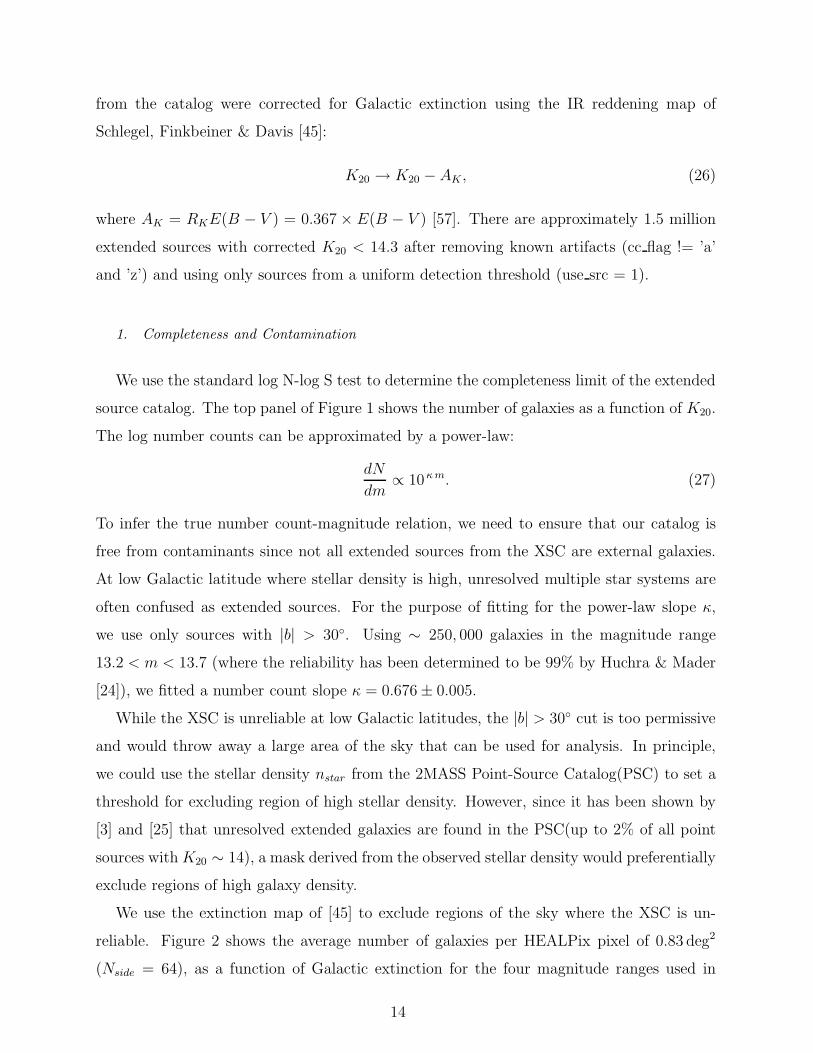
We use the standard log N-log S test to determine the completeness limit of the extended

source catalog. The top panel of Figure 1 shows the number of galaxies as a function of K20.

The log number counts can be approximated by a power-law:

dN

dm∝ 10κ m. (27)

To infer the true number count-magnitude relation, we need to ensure that our catalog is

free from contaminants since not all extended sources from the XSC are external galaxies.

At low Galactic latitude where stellar density is high, unresolved multiple star systems are

often confused as extended sources. For the purpose of fitting for the power-law slope κ,

we use only sources with |b| > 30. Using ∼ 250, 000 galaxies in the magnitude range

13.2 < m < 13.7 (where the reliability has been determined to be 99% by Huchra & Mader

[24]), we fitted a number count slope κ = 0.676 ± 0.005.

While the XSC is unreliable at low Galactic latitudes, the |b| > 30 cut is too permissive

and would throw away a large area of the sky that can be used for analysis. In principle,

we could use the stellar density nstar from the 2MASS Point-Source Catalog(PSC) to set a

threshold for excluding region of high stellar density. However, since it has been shown by

[3] and [25] that unresolved extended galaxies are found in the PSC(up to 2% of all point

sources with K20 ∼ 14), a mask derived from the observed stellar density would preferentially

exclude regions of high galaxy density.

We use the extinction map of [45] to exclude regions of the sky where the XSC is un-

reliable. Figure 2 shows the average number of galaxies per HEALPix pixel of 0.83 deg2

(Nside = 64), as a function of Galactic extinction for the four magnitude ranges used in

14

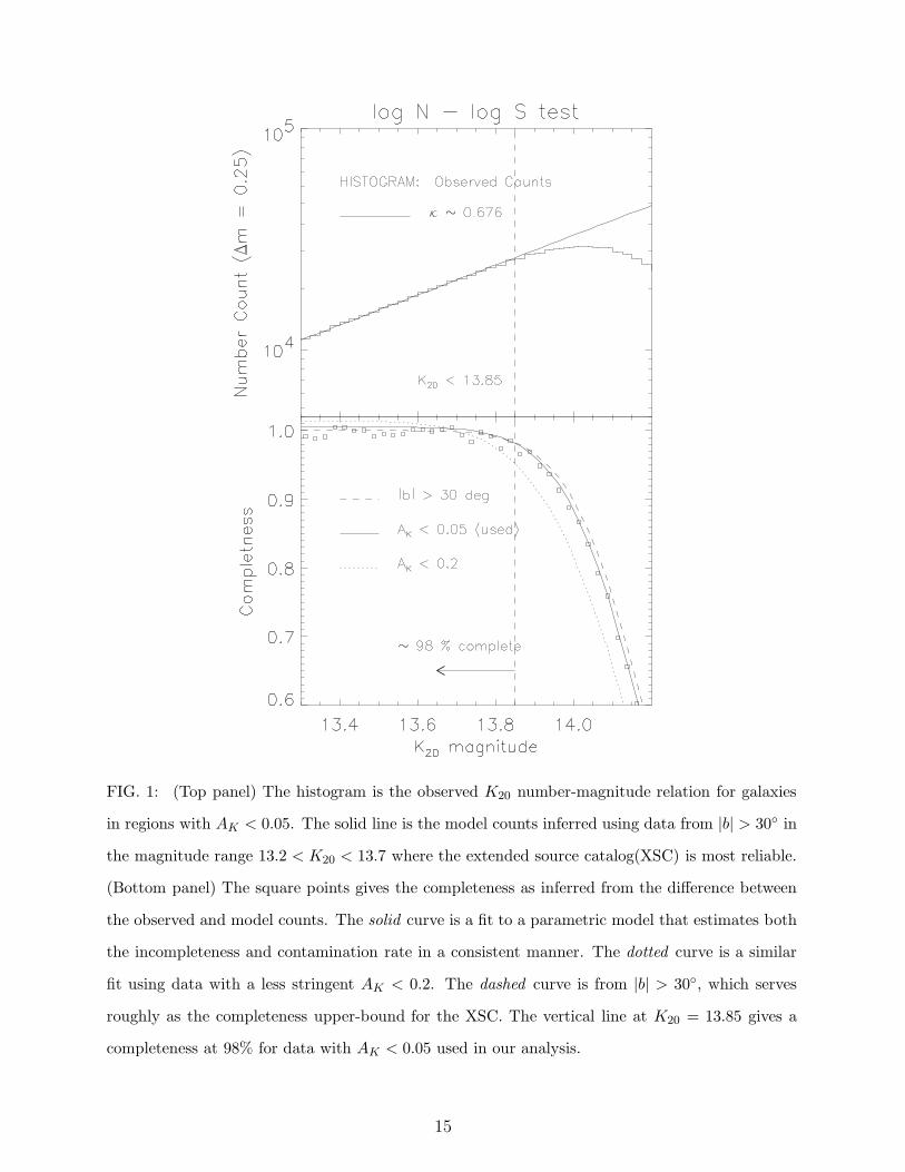
FIG. 1: (Top panel) The histogram is the observed K20 number-magnitude relation for galaxies

in regions with AK < 0.05. The solid line is the model counts inferred using data from |b| > 30 in

the magnitude range 13.2 < K20 < 13.7 where the extended source catalog(XSC) is most reliable.

(Bottom panel) The square points gives the completeness as inferred from the difference between

the observed and model counts. The solid curve is a fit to a parametric model that estimates both

the incompleteness and contamination rate in a consistent manner. The dotted curve is a similar

fit using data with a less stringent AK < 0.2. The dashed curve is from |b| > 30, which serves

roughly as the completeness upper-bound for the XSC. The vertical line at K20 = 13.85 gives a

completeness at 98% for data with AK < 0.05 used in our analysis.

15

FIG. 2: Average number of galaxies per 0.83 deg2 pixel (HEALpix Nside = 64) as a function of

extinction. For bright galaxies (K20 < 13.5), the galaxy density is constant up to extinction value

∼ 0.25. For 13.5 < K20 < 14.0, the density drops off at AK ∼ 0.65. We use only regions with

AK < 0.05 (dashed vertical line) for our analysis. Errors are estimated using jack-knife resampling.

our analysis. For bright galaxies, e.g. K20 < 13.5, the Galactic density is constant on de-

gree scales. For the faintest magnitude bin, the number density drops off at large AK for

AK beyond ∼ 0.065. We thus choose AK < 0.05 [58]. This stringent threshold excludes

∼ 99% of all regions with nstar > 5000 deg−2. Moreover, it improves the global reliability of

galaxy counts, as our flux indicator K20 for each source was corrected for Galactic extinc-

tion, which has an uncertainty that scales with AK itself. This cut reduces the number of

extended sources with K20 < 14.3 to ∼ 1 million, covering ∼ 68.7% of the sky. For the sake

of completeness, we also repeat our cross-correlation analysis for a less stringent mask with

AK < 0.1, which covers ∼ 79.0% of the sky.

Using κ = 0.676 derived from regions with |b| > 30 as a model for the true underlying

number counts, we infer the catalog completeness and contamination as a function of ap-

16

parent magnitude for the extinction cropped sky. We deduce the intercept of the linear log

counts - magnitude model by scaling the observed number counts from the |b| > 30 region

to the larger AK masked sky at the bright magnitude range 12.5 < K20 < 13.0. Essentially,

we assumed the two number count distributions are identical at those magnitudes. The

observed fractional deviation from Eq. (27)

I(m) =

(

dN

dm

κ

−dN

dm

obs) /dN

dm

κ

(28)

is positive at faint magnitudes indicating incompleteness but crosses zero to a constant

negative level towards the bright-end, which we inferred as contamination to the XSC.

Plotted in the bottom panel of Figure 1 is the completeness function C(m) ≡ 1 − I(m),

where we parametrically fitted using

I(m) = Io exp

[

−(m − m)2

2σ2

]

− Const . (29)

In Figure 1, the term Const describes the low level of excursion beyond C(m) = 1. We

obtained a ∼ 98% completeness for K20 < 13.85 and contamination rate at 0.5% level

for AK < 0.05 (solid curve). As a comparison, a less stringent threshold of AK < 0.2

(dotted curve), the completeness is ∼ 95% with contamination at 1.5%. The dashed curve

is computed using high latitude data (|b| > 30), serves roughly as the completeness upper-

bound (as a function of apparent magnitude) for the XSC.

At a low level, contaminants in the catalog merely increase the noise of our signal with

marginal systematic bias. The AK < 0.05 extinction mask is close to optimal in terms of

signal-to-noise for our cross-correlation analysis. One the other hand, catalog incompleteness

at faint magnitudes affects our ability to infer the correct redshift distribution. We use

galaxies up to K20 = 14.0 but weighted the redshift distribution at a given magnitude range

(described below) by Eq. (29).

2. Redshift Distribution

The redshift distribution of our sample was inferred from the Schechter [44] parameters

fit of the K20 luminosity function from [29]. The redshift distribution, dN/dz of galaxies

in the magnitude range mbright < m < mfaint is given by the integration of the luminosity

17

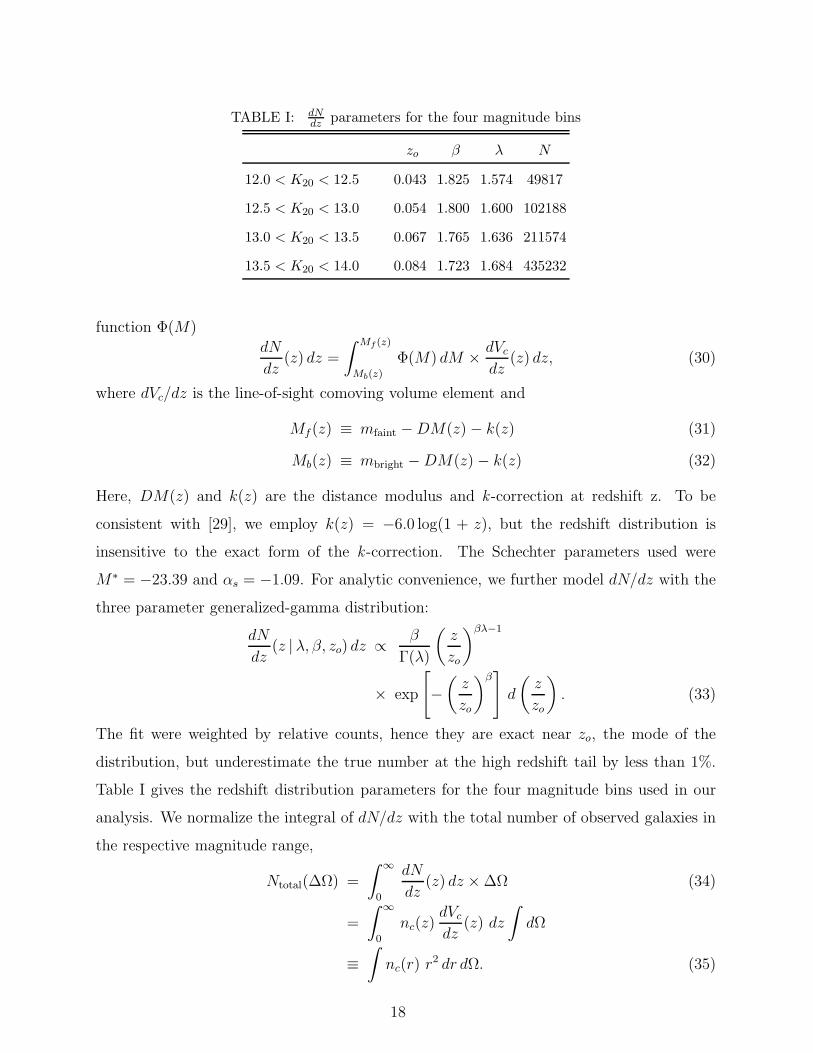
TABLE I: dNdz parameters for the four magnitude bins

zo β λ N

12.0 < K20 < 12.5 0.043 1.825 1.574 49817

12.5 < K20 < 13.0 0.054 1.800 1.600 102188

13.0 < K20 < 13.5 0.067 1.765 1.636 211574

13.5 < K20 < 14.0 0.084 1.723 1.684 435232

function Φ(M)

dN

dz(z) dz =

∫ Mf (z)

Mb(z)

Φ(M) dM ×dVc

dz(z) dz, (30)

where dVc/dz is the line-of-sight comoving volume element and

Mf (z) ≡ mfaint − DM(z) − k(z) (31)

Mb(z) ≡ mbright − DM(z) − k(z) (32)

Here, DM(z) and k(z) are the distance modulus and k -correction at redshift z. To be

consistent with [29], we employ k(z) = −6.0 log(1 + z), but the redshift distribution is

insensitive to the exact form of the k -correction. The Schechter parameters used were

M∗ = −23.39 and αs = −1.09. For analytic convenience, we further model dN/dz with the

three parameter generalized-gamma distribution:

dN

dz(z | λ, β, zo) dz ∝

β

Γ(λ)

(

z

zo

)βλ−1

× exp

[

−

(

z

zo

)β]

d

(

z

zo

)

. (33)

The fit were weighted by relative counts, hence they are exact near zo, the mode of the

distribution, but underestimate the true number at the high redshift tail by less than 1%.

Table I gives the redshift distribution parameters for the four magnitude bins used in our

analysis. We normalize the integral of dN/dz with the total number of observed galaxies in

the respective magnitude range,

Ntotal(∆Ω) =

∫

∞

0

dN

dz(z) dz × ∆Ω (34)

=

∫

∞

0

nc(z)dVc

dz(z) dz

∫

dΩ

≡

∫

nc(r) r2 dr dΩ. (35)

18

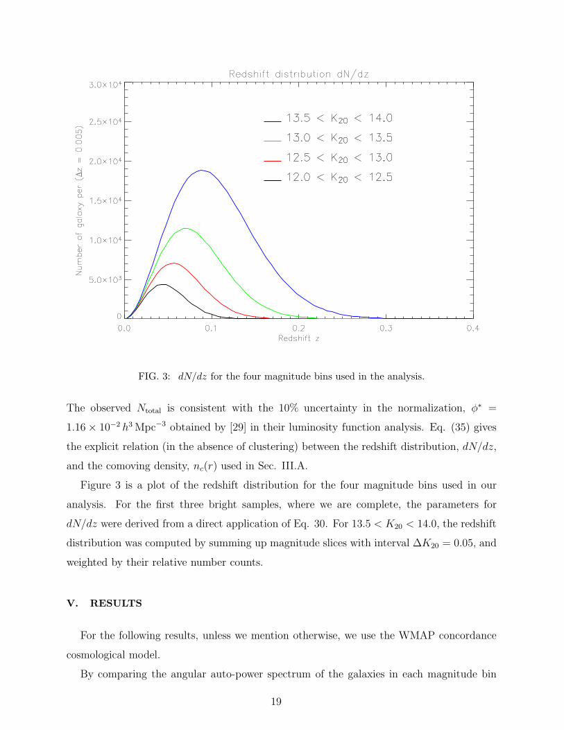
FIG. 3: dN/dz for the four magnitude bins used in the analysis.

The observed Ntotal is consistent with the 10% uncertainty in the normalization, φ∗ =

1.16 × 10−2 h3 Mpc−3 obtained by [29] in their luminosity function analysis. Eq. (35) gives

the explicit relation (in the absence of clustering) between the redshift distribution, dN/dz,

and the comoving density, nc(r) used in Sec. III.A.

Figure 3 is a plot of the redshift distribution for the four magnitude bins used in our

analysis. For the first three bright samples, where we are complete, the parameters for

dN/dz were derived from a direct application of Eq. 30. For 13.5 < K20 < 14.0, the redshift

distribution was computed by summing up magnitude slices with interval ∆K20 = 0.05, and

weighted by their relative number counts.

V. RESULTS

For the following results, unless we mention otherwise, we use the WMAP concordance

cosmological model.

By comparing the angular auto-power spectrum of the galaxies in each magnitude bin

19

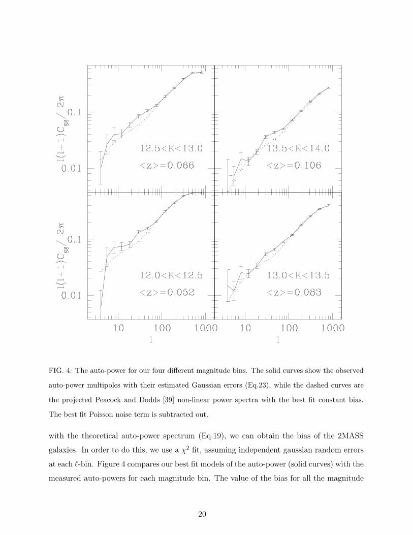
FIG. 4: The auto-power for our four different magnitude bins. The solid curves show the observed

auto-power multipoles with their estimated Gaussian errors (Eq.23), while the dashed curves are

the projected Peacock and Dodds [39] non-linear power spectra with the best fit constant bias.

The best fit Poisson noise term is subtracted out.

with the theoretical auto-power spectrum (Eq.19), we can obtain the bias of the 2MASS

galaxies. In order to do this, we use a χ2 fit, assuming independent gaussian random errors

at each ℓ-bin. Figure 4 compares our best fit models of the auto-power (solid curves) with the

measured auto-powers for each magnitude bin. The value of the bias for all the magnitude

20

bins is within

bg = 1.11 ± 0.02, (36)

which confirms our constant bias assumption[59]. Our values for the Poisson correction factor

(see Eq.19), γ, are all within 1% of 1.02. The most significant deviation of the theoretical

fit from the observed auto-power is about 30% at ℓ ∼ 30− 40. One possibility may be that

galaxy bias is larger at large (linear) scales than at the (non-linear) small scales. In order

to estimate the effect, we can limit analyses to the first 7 ℓ-bins (ℓ . 70, scales larger than

∼ 7 − 13 h−1 Mpc). This yields the estimated bias on linear scales:

bg,lin = 1.18 ± 0.08, (37)

The angular scale corresponding to ℓ = 30 − 40 is a few degrees, which is close to the

length of the 2MASS scanning stripes (6). The amplitude of deviation from the constant

bias model would require systematic fluctuations of order 10% in the number counts on that

scale. If these were due to systematic errors in the 2MASS photometric zero-point, such

fluctuations would require a magnitude error ∆m ∼ 0.06, which is significantly larger than

the calibration uncertainties in 2MASS [37]. Therefore, we will use our estimated linear bias

(Eq. 37) for the interpretation of our ISW signal, while we use the full bias estimate (Eq.

36), which is dominated by non-linear scales, to analyze our SZ signal.

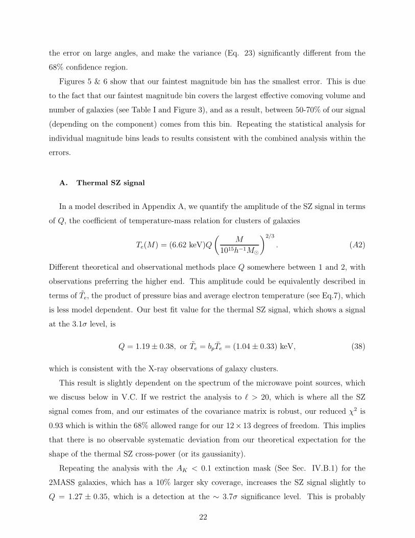
The points in Figure 5 summarize our twelve observed cross-correlation functions (3

WMAP bands × 4 magnitude bins), while Figure 6 shows the same data after subtracting out

the best fit contribution due to microwave Point Sources. We fit our theoretical model (Eq.

18) to our cross-correlation points (including only the W-band for the first 4 ℓ-bins; see Sec.

III.C), allowing for free global normalizations for the ISW, SZ and Point Source components.

The curves show this model with the best fit normalizations for these components, while

the shaded region shows the 68% uncertainty around a null hypothesis. Figure 7 shows how

individual theoretical components depend on frequency and ℓ for our faintest magnitude bin.

As we mentioned in Sec. III.C, different ℓ-bins are nearly independent. However, different

combinations of frequency bands and magnitude bins are highly correlated and we use the

full covariance matrix which we obtain from the data itself (see III.C) for our χ2 analysis.

The apparent dispersion in our data points for the first 4-5 ℓ-bins is smaller than what

we expect from gaussian statistics (the shaded regions in Figures 5 and 6). This may be due

to the non-gaussian nature of the systematics (observational or Galactic), which dominate

21

the error on large angles, and make the variance (Eq. 23) significantly different from the

68% confidence region.

Figures 5 & 6 show that our faintest magnitude bin has the smallest error. This is due

to the fact that our faintest magnitude bin covers the largest effective comoving volume and

number of galaxies (see Table I and Figure 3), and as a result, between 50-70% of our signal

(depending on the component) comes from this bin. Repeating the statistical analysis for

individual magnitude bins leads to results consistent with the combined analysis within the

errors.

A. Thermal SZ signal

In a model described in Appendix A, we quantify the amplitude of the SZ signal in terms

of Q, the coefficient of temperature-mass relation for clusters of galaxies

Te(M) = (6.62 keV)Q

(

M

1015h−1M⊙

)2/3

. (A2)

Different theoretical and observational methods place Q somewhere between 1 and 2, with

observations preferring the higher end. This amplitude could be equivalently described in

terms of Te, the product of pressure bias and average electron temperature (see Eq.7), which

is less model dependent. Our best fit value for the thermal SZ signal, which shows a signal

at the 3.1σ level, is

Q = 1.19 ± 0.38, or Te = bpTe = (1.04 ± 0.33) keV, (38)

which is consistent with the X-ray observations of galaxy clusters.

This result is slightly dependent on the spectrum of the microwave point sources, which

we discuss below in V.C. If we restrict the analysis to ℓ > 20, which is where all the SZ

signal comes from, and our estimates of the covariance matrix is robust, our reduced χ2 is

0.93 which is within the 68% allowed range for our 12× 13 degrees of freedom. This implies

that there is no observable systematic deviation from our theoretical expectation for the

shape of the thermal SZ cross-power (or its gaussianity).

Repeating the analysis with the AK < 0.1 extinction mask (See Sec. IV.B.1) for the

2MASS galaxies, which has a 10% larger sky coverage, increases the SZ signal slightly to

Q = 1.27 ± 0.35, which is a detection at the ∼ 3.7σ significance level. This is probably

22

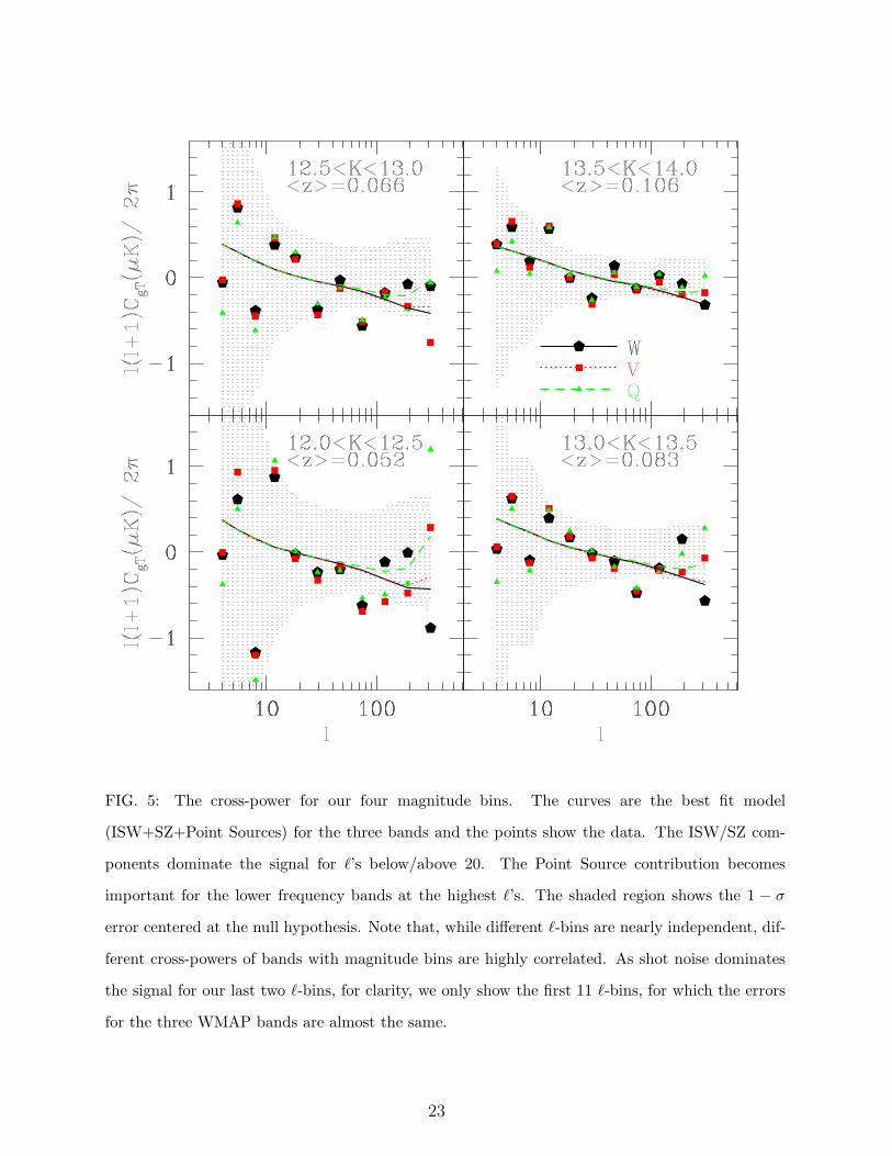
FIG. 5: The cross-power for our four magnitude bins. The curves are the best fit model

(ISW+SZ+Point Sources) for the three bands and the points show the data. The ISW/SZ com-

ponents dominate the signal for ℓ’s below/above 20. The Point Source contribution becomes

important for the lower frequency bands at the highest ℓ’s. The shaded region shows the 1 − σ

error centered at the null hypothesis. Note that, while different ℓ-bins are nearly independent, dif-

ferent cross-powers of bands with magnitude bins are highly correlated. As shot noise dominates

the signal for our last two ℓ-bins, for clarity, we only show the first 11 ℓ-bins, for which the errors

for the three WMAP bands are almost the same.

23

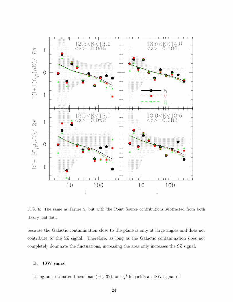
FIG. 6: The same as Figure 5, but with the Point Source contributions subtracted from both

theory and data.

because the Galactic contamination close to the plane is only at large angles and does not

contribute to the SZ signal. Therefore, as long as the Galactic contamination does not

completely dominate the fluctuations, increasing the area only increases the SZ signal.

B. ISW signal

Using our estimated linear bias (Eq. 37), our χ2 fit yields an ISW signal of

24

FIG. 7: Different components of our best fit theoretical cross-power model, compared with the

data for our faintest magnitude bin (13.5 < K < 14). The dotted(red) curves show the ISW

component, while the short-dashed(green) and long-dashed(blue) curves are the SZ and Point

Source components respectively. The black curves show the sum of the theoretical components,

while the points are the observed cross-power data.

ISW = 1.49 ± 0.61 (39)

× concordance model prediction,

a 2.5σ detection of a cross-correlation. As with the previous cross-correlation analyses[8,

16, 17, 38], this is consistent with the predictions of the concordance ΛCDM paradigm.

25

However, among the three signals that we try to constrain, the ISW signal is the most

difficult to extract, because almost all the signal comes from ℓ < 20, given our redshift

distribution. For such low multipoles, there are several potential difficulties:

1- The small Galactic contamination or observational systematics in 2MASS may dom-

inate the fluctuations in the projected galaxy density at low multipoles and wipe out the

signal. However, since we use the observed auto-power of 2MASS galaxies for our error

estimates, this effect, which does contribute to the auto-power (and not to the signal), is

included in our error.

2- Our covariance estimator loses its accuracy as the cosmic variance becomes important

at low multipoles (see III.C). A random error in the covariance matrix can systematically

increase the χ2 and hence decrease the estimated error of our signal. However, our reduced

χ2 is 0.88, which is in fact on the low side (although within 1σ) of the expected values for

124 degrees of freedom [60] (remember that we only used the W band for the first 4 ℓ-bins).

Assuming gaussian statistics, this implies that we do not significantly underestimate our

error.

3- Possible Galactic contamination in WMAP may correlate with Galactic contamination

in 2MASS at low multipoles, which may lead to a fake positive signal. However, the largest

contribution of Galactic foreground is visible in the Q-band [6], and our low ℓ multipoles

have in fact a lower amplitude in Q band. Although this probably shows a large error due

to contamination in the Q-band amplitude, the fact that this is lower than the amplitude of

V and W bands implies that our main signal is not contaminated. Because of the reasons

mentioned in III.C, we only use the W-band information for ℓ < 14.

Using the less stringent extinction mask, AK < 0.1 (see IV.B.1), for the 2MASS sources

yields a signal of ISW= 1.9±1.1, which is a lower signal to noise detection at the 1.7σ level.

This is probably due to the fact that most of the ISW signal comes from angles larger than

∼ 10, which is highly contaminated in regions close to the Galactic Plane.

Finally, we should mention that since the ISW signal comes from small ℓ’s, while the SZ

and point source signals come from large ℓ’s (See Figure 7), there is a small correlation (less

than 10%) between the ISW and other signals.

26

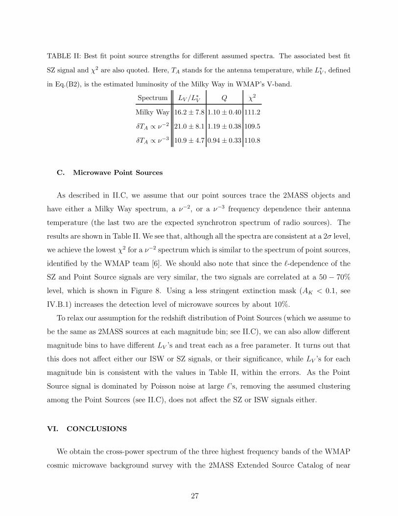
TABLE II: Best fit point source strengths for different assumed spectra. The associated best fit

SZ signal and χ2 are also quoted. Here, TA stands for the antenna temperature, while L∗

V , defined

in Eq.(B2), is the estimated luminosity of the Milky Way in WMAP’s V-band.

Spectrum LV /L∗

V Q χ2

Milky Way 16.2 ± 7.8 1.10 ± 0.40 111.2

δTA ∝ ν−2 21.0 ± 8.1 1.19 ± 0.38 109.5

δTA ∝ ν−3 10.9 ± 4.7 0.94 ± 0.33 110.8

C. Microwave Point Sources

As described in II.C, we assume that our point sources trace the 2MASS objects and

have either a Milky Way spectrum, a ν−2, or a ν−3 frequency dependence their antenna

temperature (the last two are the expected synchrotron spectrum of radio sources). The

results are shown in Table II. We see that, although all the spectra are consistent at a 2σ level,

we achieve the lowest χ2 for a ν−2 spectrum which is similar to the spectrum of point sources,

identified by the WMAP team [6]. We should also note that since the ℓ-dependence of the

SZ and Point Source signals are very similar, the two signals are correlated at a 50 − 70%

level, which is shown in Figure 8. Using a less stringent extinction mask (AK < 0.1, see

IV.B.1) increases the detection level of microwave sources by about 10%.

To relax our assumption for the redshift distribution of Point Sources (which we assume to

be the same as 2MASS sources at each magnitude bin; see II.C), we can also allow different

magnitude bins to have different LV ’s and treat each as a free parameter. It turns out that

this does not affect either our ISW or SZ signals, or their significance, while LV ’s for each

magnitude bin is consistent with the values in Table II, within the errors. As the Point

Source signal is dominated by Poisson noise at large ℓ’s, removing the assumed clustering

among the Point Sources (see II.C), does not affect the SZ or ISW signals either.

VI. CONCLUSIONS

We obtain the cross-power spectrum of the three highest frequency bands of the WMAP

cosmic microwave background survey with the 2MASS Extended Source Catalog of near

27

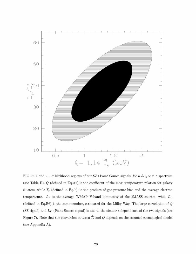
FIG. 8: 1 and 2 − σ likelihood regions of our SZ+Point Source signals, for a δTA ∝ ν−2 spectrum

(see Table II). Q (defined in Eq.A2) is the coefficient of the mass-temperature relation for galaxy

clusters, while Te (defined in Eq.7), is the product of gas pressure bias and the average electron

temperature. LV is the average WMAP V-band luminosity of the 2MASS sources, while L∗

V

(defined in Eq.B6) is the same number, estimated for the Milky Way. The large correlation of Q

(SZ signal) and LV (Point Source signal) is due to the similar ℓ-dependence of the two signals (see

Figure 7). Note that the conversion between Te and Q depends on the assumed cosmological model

(see Appendix A).

28

infrared galaxies. We detect an ISW signal at the ∼ 2.5σ level, which confirms the presence

of a dark energy, at a level consistent with the WMAP concordance cosmology. We also find

evidence for an anti-correlation at small angles (large ℓ’s), which we attribute to thermal

SZ. The amplitude is at 3.1 − 3.7σ level and is consistent with the X-ray observations of

galaxy clusters. Finally, we see a signal for microwave Point Sources at the 2.6σ level.

We’ve seen that the completeness limit of the extended source catalog is between 13.5

and 14 in K. However, matches with SDSS show that there are many unresolved sources

in the 2MASS Point Source Catalog (PSC) that are in fact galaxies. If we can select out

galaxies in the PSC, perhaps by their distinctive colors, we should be able to push the sample

at least half a magnitude fainter than we have done here, probing higher redshifts with a

substantially larger sample.

Future wide-angle surveys of galaxies should be particularly valuable for cross-correlation

with the WMAP data, especially as the latter gains signal-to-noise ratio in further data

releases. The Pan-STARRS project [27] for example, should yield a multi-color galaxy

catalog to 25th mag or even fainter over 20,000 square degrees or more of the sky well before

the end of the decade; it will more directly probe the redshift range in which the SZ and

ISW kernels peak, and therefore should be particularly valuable for cross-correlating with

WMAP and other CMB experiments.

Acknowledgments

NA wishes to thank David N. Spergel for the supervision of this project and useful dis-

cussions. We would also like to thank Eiichiro Komatsu, Andrey Kravstov and Christopher

Hirata for illuminating discussions and helpful suggestions, Doug Finkbeiner for help on the

analysis of WMAP temperature maps, and R.M. Cutri and Mike Skrutskie on the 2MASS

dataset. MAS acknowledges the support of NSF grants ASF-0071091 and AST-0307409.

[1] Abell, G.O., Corwin, H., Olwin, R., 1989, ApJS, 70, 1

[2] Afshordi, N., & Cen, R. 2002, ApJ, 564, 669

[3] Bell, E.F., et al. 2003, ApJS, 149, 289

[4] Bennett, C. et al. 1996, ApJ, 464, L1

29

[5] Bennett, C.L. et al. 2003, ApJS, 148, 1; The public data and other WMAP papers are available

at http://lambda.gsfc.nasa.gov/product/map

[6] Bennett, C.L. et al. 2003, ApJS, 148, 97

[7] Boughn, S. P., Private Communication.

[8] Boughn, S. P. & Crittenden, R. G., Phys. Rev. Lett. 88, 021302 (2002)

[9] Boughn, S. P. & Crittenden, R. G. 2003, astro-ph/0305001

[10] Condon, J. et al. 1998, Astron. J. 115, 1693

[11] Cooray, A. 2002, Phys. Rev. D, 65, 103510

[12] Corasaniti, P.S. et al. 2003, PRL, 90, 091303

[13] Crittenden, R.G., & Turok, N. 1996, PRL, 76, 575

[14] Diego. J.M., Silk J., & Sliwa 2003, MNRAS, 346, 940

[15] Efstathiou, G. 2003, astro-ph/0307515

[16] Fosalba P., & Gaztanaga E. 2003, astro-ph/0305468

[17] Fosalba P., Gaztanaga E., & Castander, F.J. 2003, ApJ, 597L, 89

[18] Gorski, K. M., Hivon, E., & Wandelt, B. D. 1998, in Evolution of Large-Scale Structure: From

Recombination to Garching

[19] Gunn, J., Gott, J. 1972, ApJ, 176, 1

[20] Hernandez-Monteagudo, C., & Rubino-Martin, J.A. 2003, astro-ph/0305606

[21] Hivon, E., Gorski, K. M., Netterfield, C. B., Crill, B. P., Prunet, S., & Hansen, F. 2002, ApJ,

567, 2

[22] Hinshaw, G., et al. 2003, ApJS, 148, 135

[23] Hu, W. & Dodelson, S. 2002, ARA&A, 40, 171

[24] Huchra, J & Mader, J (2000) at http://cfa-www.harvard.edu/∼huchra/2mass/verify.htm

[25] Ivezic, Z. et al. in IAU Colloquium 184: AGN Surveys, 18-22 June 2001, Byurakan(Armenia)

[26] Jarrett, T.H., et al. 2000, AJ, 119, 2498

[27] Kaiser et al. 2002, SPIE, 4836, 154

[28] Kesden, K., Kamionkowski, M., & Cooray, A. 2003, astro-ph/0306597

[29] Kochanek, C.S., et al. 2001, ApJ 560, 566

[30] Kogut, C.L. et al. 2003a, ApJS, 148, 161

[31] Komatsu, E., Afshordi, N., & Seljak, U. 2003, in preparation

[32] Komatsu, E., & Seljak, U. 2001, MNRAS, 327, 1353

30

[33] Limber, D.N. 1954, ApJ , 119, 655

[34] Maddox, S. J., et al. 1990, MNRAS, 242, 43

[35] Maller, A. H., et al. 2003, astro-ph/0304005

[36] Myers, A.D., Shanks, T. Outram, P.J., Wolfendale, A.W. 2003, astro-ph/0306180

[37] Nikolaev, S., et al. 2000, AJ, 120, 3340

[38] Nolta, M.R., et al. 2003, astro-ph/030597

[39] Peacock, J.A., & Dodds, S.J. 1996, MNRAS, 280L, 19

[40] Peebles, P. J. E., & Ratra, B. 2003, Rev.Mod.Phys. 75, 599

[41] Peiris, H., & Spergel, D.N. 2000, ApJ, 540, 605

[42] Refregier A., Komatsu E., Spergel D. N., Pen U., 2000, Phys. Rev. D, 61,123001

[43] Sachs, R. K. & Wolfe, A. M. 1967, ApJ, 147, 73

[44] Schechter, P. 1976, ApJ 203, 296.

[45] Schlegel, D.J., Finkbeiner, D.P. & Davis, M. 1998, ApJ 500, 525.

[46] Scranton, R. et al. 2003, astro-ph/0305337

[47] Seljak, U. & Zaldarriaga, M. 1996, ApJ, 469, 437

[48] Sheth, R. K. & Tormen, G. 1999, MNRAS, 308, 119

[49] Spergel, D.N. et al. 2003, ApJS, 148, 175

[50] Skrutskie et al. 1997, in The Impact of Large Scale Near-IR Sky Survey, ed. F. Garzon et al.

(Dordrecht: Kluwer), 187

[51] Tegmark, M. 1997, Phys. Rev. D, 56, 4514

[52] York, D.G. et al. 2000, AJ, 120, 1579

[53] Zhang, P., & Pen, U. 2001, ApJ, 549, 18

[54] Zel’dovich Y.B., & Sunyaev, R.A. 1969, ApSpSci, 4, 129.

[55] We thank Doug Finkbeiner for extracting the fluxes of Andromeda in WMAP temperature

maps.

[56] We thank Eiichiro Komatsu for pointing out this identity.

[57] This is different from RK = 0.35 used by [29] whose luminosity function parameters we use

to estimate the redshift distribution, but the median difference of extinction derived between

the two is small(< 0.002 mag).

[58] This is also the level chosen by [35] for their auto-correlation analysis of the XSC.

[59] Given that the galaxy distribution is non-linear and non-gaussian, the χ2 fit is not the optimal

31

bias estimator. However, the fact that the biases for different bins are so close implies that the

error in bias, as we see below, is much smaller than the error in our cross-correlation signal

and so is negligible.

[60] A low χ2 is to be expected if we overestimate the noise in the ISW signal. In particular, this

could be the case if the CMB power is suppressed on large angles. This would increase the

significance of an ISW detection at such scales. This effect is elaborated in [28]

APPENDIX A: SEMI-ANALYTICAL ESTIMATE OF SZ SIGNAL

In order to find Te (defined in Eq.7) we need an expression for the dependence of the

electron pressure overdensity on the matter overdensity. As the shock-heated gas in clusters

of galaxies has keV scale temperatures and constitutes about 5− 10% of the baryonic mass

of the universe, its contribution to the average pressure of the universe is significantly higher

than the photo-ionized inter-galactic medium (at temperatures of a few eV). Thus, the

average electron pressure in a large region of space with average density ρ(1 + δm) is given

by

δpe ≃ne

ρ

∫

dM · M · kB[Te(M ; ρ)∂n(M ; ρ)

∂ρ+ n(M ; ρ)

∂Te(M ; ρ)

∂ρ]ρδm

=ne

ρ

∫

dM · M · n(M ; ρ)[kBTe(M ; ρ)][b(M) +∂ log Te

∂ log ρ]δm, (A1)

where n(M ; ρ) and Te(M ; ρ) are the mass function and temperature-mass relation of galaxy

clusters respectively. Also, b(M) = ∂ log n(M ;ρ)∂ log ρ

is the bias factor for haloes of virial mass M

(= M200; mass within the sphere with the overdensity of 200 relative to the critical density).

For our analysis, we use the Sheth & Tormen analytic form [48], for n(M) and b(M), which

is optimized to fit numerical N-body simulations.

We can use theoretical works on the cluster mass-temperature relation (which assume

equipartition among thermal and kinetic energies of different components in the intra-cluster

medium) to find Te(M), (e.g. [2])

kBTe(M)

mp≃ (0.32Q)(2πGHM)2/3

⇒ Te(M) = (6.62 keV)Q

(

M

1015h−1M⊙

)2/3

,

while 1 < Q < 2 (A2)

32

for massive clusters, where H = 100h km s−1/ Mpc is the (local) Hubble constant. Although

there is controversy on the value of the normalization Q (see e.g. [32] and references there

in), [2] argue that, as long as there are no significant ongoing astrophysical feed-back or

cooling (i.e., as long the evolution is adiabatic), the dependence on H and M should be the

same. Combining this with the local comoving continuity equation

3(H + δH) = −˙ρ

ρ− δm, (A3)

yields∂ log Te

∂ log ρ=

2

3

∂ log H

∂ log ρ= −

2D

9DH, (A4)

where D is the linear growth factor.

One may think is that observations may be the most reliable way of constraining Q in

Eq.(A2). However, almost all the observational signatures of the hot gas in the intra-cluster

medium come from the X-ray observations which systematically choose the regions with

high gas density. With this in mind, we should mention that while observations prefer a

value of Q close to 1.7, numerical simulations and analytic estimates prefer values closer

to 1.2[2]. For our analysis, we treat Q as a free parameter which we constrain using our

cross-correlation data (see Sec. V.A).

Putting all the pieces together, we end up with the following expression for Te

Te = (0.32 Q)(2πGH)2/3

×∫

dνfST [ν]M2/3[bST (ν) − 2D9DH

], (A5)

ν(M) = δc

σ(M),

where σ(M) is the variance of linear mass overdensity within a sphere that contains mass M

of unperturbed density, while δc ≃ 1.68 is the spherical top-hot linear growth threshold[19].

fST and bST are defined in [48]. For the WMAP concordance cosmological model[5], this

integral can be evaluated to give

Te = bpTe = (0.88 Q) keV. (A6)

The above simple treatment of the SZ signal fails at scales comparable to the minimum

distance between clusters, where the average gas pressure does not follow the average matter

density [42, 53], which leads to a scale-dependent pressure bias. Moreover, efficient galaxy

33

formation removes the hot gas from the intra-cluster medium, which causes Eq.A1 to over-

estimate the SZ signal. As this paper mainly focuses on the observational aspects of our

detection, we delay addressing these issues into a further publication[31]. The preliminary

results seem to be consistent with the above simple treatment at the 20% level.

APPENDIX B: MICROWAVE LUMINOSITIES OF THE ANDROMEDA

GALAXY AND THE MILKY WAY

First we derive how much the flux received by a microwave source at distance dL and

observed solid angle δΩ affects the observed CMB temperature. The apparent change in the

black-body temperature is obtained by

δΩ · δ

[

4π(~/c2)ν3∆ν

exp[hν/(kBTCMB

)] − 1

]

=L

4πd2L

. (B1)

The left hand side of Eq.(B1) is the change in the Planck intensity, where ν and ∆ν are

the detector frequency and band width respectively. The right hand side is the observed

Microwave flux. Defining x as the frequency in units of kBTCMB

/h, Eq.(B1) yields

δT

T=

4π2~

3c2

(kBTCMB

)4·sinh2(x/2)

x4∆x·

L

δΩd2L

. (B2)

To obtain the microwave luminosity of Milky Way, we assume an optically and geomet-

rically thin disk, with a microwave emissivity, ǫ, which is constant across its thickness and

falls as ǫ0 exp(−r/r0) with the distance, r, from its center. The disk thickness is 2H ≪ r,

while we assume r0 ≃ 5 kpc, our distance from the Galactic center is r ≃ 8.5 kpc, and our

vertical distance from the center of the disk is z. Integrating Eq.(B2) over the disk thickness

leads to the cosecant law for the Galactic emission

δT

T(b; r) =

4π2~

3c2

(kBTCMB

)4·sinh2(x/2)

x4∆x· ǫ0e

−r/r0(H| csc b| − z csc b), (B3)

where b is Galactic latitude. Integrating ǫ(r) over the disk volume gives the total luminosity

of the Milky Way

L = 2H

∫

2πrdr ǫ0e−r/r0 = 4πHr2

0ǫ0. (B4)

Combining Eqs.B3 and B4, we can obtain the total luminosity of Milky Way from the

observed Galactic emission

L = r20e

r/r0 ·(kBT

CMB)4

2π~3c2·

x4∆x

sinh2(x/2)· | sin b|

[

δT

T(b; r) +

δT

T(−b; r)

]

. (B5)

34

Figure 7 in [6] gives the cosecant law for the Galactic emission in different WMAP bands.

Using this information in Eq.(B5) (after conversion into thermodynamic units) gives the

luminosity of the Milky Way in WMAP bands

L∗

Q = 1.7 × 1037 erg s−1,

L∗

V = 3.0 × 1037 erg s−1,

and L∗

W = 1.0 × 1038 erg s−1. (B6)

To confirm these values, we can use Eq.(B2) and the observed integrated flux of the

Andromeda (M31) galaxy in the WMAP maps to obtain its microwave luminosity

LM31,Q = 2.1 × 1037 erg s−1,

LM31,V = 5.3 × 1037 erg s−1,

and LM31,W = 1.6 × 1038 erg s−1. (B7)

We see that these values are larger, but within 50%, of the Milky Way microwave luminosi-

ties.

35