CRMW Strategic Monitoring Plan 2008

STRATEGIC MONITORING AND RESEARCH PLAN

FOR THE CEDAR RIVER MUNICIPAL WATERSHED

January, 2008

Monitoring and Research Inter-Disciplinary Team Sally Nickelson (Team Leader – Fish and Wildlife)

Todd Bohle (Hydrology) Melissa Borsting (Forest Ecology) David Chapin (Fish and Wildlife)

Mark Joselyn, Duncan Munro (Information Technology)

City of Seattle Seattle Public Utilities

Watershed Services Division Watershed Ecosystems Section

2

Table of Contents EXECUTIVE SUMMARY .........................................................................................................................................4

1.0 INTRODUCTION.........................................................................................................................................7 1.1 BACKGROUND .............................................................................................................................................7 1.2 MONITORING AND THE CEDAR RIVER WATERSHED HABITAT CONSERVATION PLAN .................................7 1.3 PURPOSE OF STRATEGIC MONITORING AND RESEARCH PLAN .....................................................................8

2.0 FRAMING STRATEGIC MONITORING.................................................................................................9 2.1 ASSET MANAGEMENT FRAMEWORK ...........................................................................................................9 2.2 RISKS, UNCERTAINTIES, AND THREATS.......................................................................................................9 2.3 ADAPTIVE MANAGEMENT .........................................................................................................................10

2.3.1 Passive versus Active Adaptive Management ......................................................................................11 2.4 RESEARCH.................................................................................................................................................12

3.0 OBJECTIVES, SCOPE, AND OVERALL APPROACH........................................................................15 3.1 MONITORING AND RESEARCH OBJECTIVES ...............................................................................................15 3.2 SCOPE AND OVERALL APPROACH .............................................................................................................16

3.2.1 Species-Specific Monitoring ................................................................................................................18 3.2.2 Threat Monitoring ...............................................................................................................................18 3.2.3 Long-term Ecological Trend Monitoring.............................................................................................19 3.2.4 Project-Specific Monitoring ................................................................................................................21

4.0 STANDARDS, GUIDELINES, AND RECOMMENDATIONS FOR MONITORING PLANS..........22 4.1 STANDARDS FOR MONITORING PLANS ......................................................................................................23 4.2 GUIDELINES FOR MONITORING PLANS ......................................................................................................23

4.2.1 Information Review..............................................................................................................................23 4.2.2 Monitoring Design and Procedures.....................................................................................................24

5.0 INTEGRATION/COORDINATION OF MONITORING EFFORTS...................................................24 5.1 INTEGRATION AND COORDINATION...........................................................................................................24 5.2 RELATIONSHIPS.........................................................................................................................................26 5.3 TRACKING MONITORING NEEDS ...............................................................................................................27 5.4 RESPONSIBILITIES .....................................................................................................................................29

6.0 PRIORITIZATION OF MONITORING EFFORTS ..............................................................................36 6.1 PRIORITIZATION OF SPECIES MONITORING................................................................................................37 6.2 PRIORITIZATION OF THREAT MONITORING................................................................................................37 6.3 PRIORITIZATION OF LONG-TERM ECOLOGICAL TREND MONITORING........................................................38 6.4 PRIORITIZATION OF PROJECT EFFECTIVENESS MONITORING .....................................................................38

7.0 FUNDING ....................................................................................................................................................40 7.1 HCP COMPLIANCE ....................................................................................................................................40 7.2 BUDGETS AND FUNDING GAPS ..................................................................................................................41 7.3 FUNDING OPTIONS ....................................................................................................................................41

8.0 ONGOING OVERSIGHT AND COORDINATION ...............................................................................42 8.1 MONITORING STRATEGY AND PLAN REVIEW ............................................................................................42 8.2 INFORMATION EXCHANGE.........................................................................................................................42 8.3 FUTURE CHANGES/ADAPTIVE MANAGEMENT...........................................................................................43

9.0 RECOMMENDATIONS AND NEXT STEPS .........................................................................................43

10.0 REFERENCES............................................................................................................................................45

3

List of Figures Figure 1. Decision process to determine the appropriate level of monitoring….……………. . 14 Figure 2. Overview of monitoring components for the CRMW……………………………… 17 Figure 3. Relationships between CRMW ID Teams and guiding documents and plans……… 27 Figure 4. Prioritization process for restoration project monitoring…………………………… 40 List of Tables Table 1. Aquatic project effectiveness monitoring, estimated needs by year and project……. 30 Table 2. Riparian forest project effectiveness monitoring, estimated needs by year and project. 31 Table 3. Upland forest project effectiveness monitoring, estimated needs by year and project.. 32 Table 4. Long-term ecological trend monitoring, estimated needs by year……………………. 33 Table 5. Estimated combined monitoring needs……………………………………………….. 34 Table 6. HCP defined monitoring categories and subcategories and the responsible team or work group…………………………………………………………………………………………… 35 Table 7. Potential monitoring needs not specifically addressed in HCP………………………. 36 Appendices Appendix A: Monitoring Overview Appendix B: Uncertainty and Adaptive Management Appendix C: Current and Planned Research Projects in the CRMW Appendix D: Long-term Ecological Trend Monitoring Appendix E: Water Quality Monitoring Appendix F: Road Surface Erosion Monitoring Study Plan

4

EXECUTIVE SUMMARY This Strategic Monitoring and Research Plan for the Cedar River Municipal Watershed (CRMW) provides a general overview of monitoring, including definitions, reasons to monitor, and key components to include in a monitoring program. It also provides a framework, approach, standards, guidelines, and recommendations for all monitoring activities within the CRMW. It includes recommendations for integration, coordination, and prioritization of monitoring activities within the CRMW. Finally, we review ongoing and planned research projects. Monitoring in the CRMW will focus on key risks, uncertainties, and threats. The Ecosystems Section, Watershed Services Division of Seattle Public Utilities, has defined risks as undesirable outcomes from a management action or technique, or from the decision to do no restoration. Uncertainties are defined as limited knowledge of ecological processes or outcomes of restoration/management techniques. Threats are defined as negative effects from tangible sources (e.g., invasive species). Monitoring must inform our future management decisions and actions in the face of these risks, uncertainties, and threats. As such, monitoring will focus on those actions or techniques that will be repeated and will utilize indicators that will provide timely information useful in the design of future restoration treatments. Adaptive management, in which learning is explicitly defined as a project goal, is an essential component of the Cedar River Watershed Habitat Conservation Plan (CRW-HCP) because of the uncertainty involved with ecosystem restoration and the experimental nature of some restoration techniques. Two types of adaptive management are discussed and are contrasted with typical natural resources management and strict ecological research.

• Passive adaptive management entails monitoring a single type of management activity or technique. The choice of technique is based on what managers believe to be the most likely model for how a prescription will affect the ecosystem. This is usually a conservative approach, involving a small risk of adverse environmental impact.

• Active adaptive management is designed to provide more information about the ecosystem being modified by using a range of treatments. However, it may involve greater risk of adverse impact and requires additional technical rigor, thus greater effort and resources. The advantage of active adaptive management is that a range of prescriptions can be evaluated for success in achieving management objectives, resulting in a greater likelihood of interpretable results.

There may also be situations where a strict research design is required to answer very specific questions. This would involve the highest level of scientific rigor, and would generally be carried out on a small scale over shorter time frames, often in conjunction with partners from institutions such as the University of Washington (UW), the National Oceanic and Atmospheric Administration (NOAA) Fisheries, or the US Geological Survey (USGS). Monitoring in the CRMW will address four main components, all of which will contribute to future management and restoration decisions: 1. Species-specific monitoring is largely outlined in the HCP, and includes bull trout, northern

spotted owl, marbled murrelet, and common loon. Additional species may also be monitored

5

in support of the HCP commitment to protect and restore biodiversity, to monitor restoration project effectiveness, and to provide validation that the anticipated species benefits are in fact occurring.

2. Threat Monitoring will identify and track key ecological threats in a timely manner, when

they can still be minimized with relatively small outlay of resources. 3. Long-term ecological trends are measured on a watershed-wide scale to document the range

of conditions and variability within the watershed in a statistically valid manner. In addition, we will monitor the processes, condition, extent, and location of specific habitat types, and responses to threats such as invasive plants. We will use a combination of remotely-sensed image data and ground-based data collected on a watershed-wide system of upland and riparian forest permanent sample plots (PSPs) and permanent monitoring reaches (PMRs) to monitor selected stream reaches.

4. Project-specific monitoring will include compliance, effectiveness, and adaptive

management components for all categories of restoration projects (upland, riparian, aquatic, and roads). Some projects may also include validation monitoring, where assumptions about cause and effect relationships are tested. It is critical that monitoring data have the widest possible area of inference. Consequently, most project monitoring designs will involve sampling that encompasses a number of different projects of similar type, rather than designing a unique monitoring program for each project.

The Monitoring and Research Inter-disciplinary (ID) Team developed a series of standards, guidelines, and recommendations for use by restoration project teams. Essential components of monitoring strategies and plans include:

• defining clear restoration objectives and desired future conditions; • focusing monitoring on key risks, uncertainties, and threats; • developing key questions and scientific hypotheses; • clearly relating the monitoring goal to the project goals; • identifying the key ecological processes; • identifying indicator variables that will respond in a short time frame, and linking them to

the ecological processes, restoration objectives, and hypotheses; • developing conceptual models that illustrate the relationship of the key processes and

indicators; • conducting literature reviews; • documenting and referencing sampling protocols; • addressing quality control; • estimating monitoring costs and delineating funding sources; • use of common protocols, documentation and centralized data storage, and • clearly linking monitoring results to future decision making.

We recommend methods to coordinate and integrate monitoring among projects, including ecological, spatial, temporal, and methodological integration. A framework for how restoration and project ID teams can prioritize among monitoring efforts is provided. Risk of adverse outcome, level of scientific uncertainty about ecological processes or management outcomes,

6

value of results to inform future management decisions, and project and monitoring costs will all be taken into account by the project teams during prioritization. There are a number of possible funding options for monitoring efforts that do not have a specific budget commitment in the HCP. They include: 1) dedicating a percentage of the project budget to baseline and immediate post-project monitoring; 2) pooling funding across several HCP budgets to address a coordinated series of projects; 3) establishing collaborative projects; 4) creating cost shares with universities, agencies, or individuals; 5) utilizing grant opportunities; 6) using volunteers and interns; and 7) utilizing revenues (if any) generated from ecological thinning. A policy decision for ongoing funding will be required if all appropriate monitoring will be conducted. Ongoing responsibilities of the Monitoring and Research ID Team will include development of broad overall monitoring strategies, support and consultation to other teams during monitoring plan development; review of monitoring strategies and plans; identification of overlapping efforts; recommendations on data collection, integration, and coordination; coordination of information exchange about ongoing and upcoming monitoring efforts; and developing and managing a centralized database that tracks the monitoring schedule for all monitoring efforts within the CRMW.

7

1.0 INTRODUCTION 1.1 Background Monitoring is essential to track ecological changes through time, document results of both management interventions and decisions not to intervene, and manage complex ecosystems that are poorly understood and characterized by uncertainty, crises, and surprises (Gunderson 2003). Monitoring can take many forms and include numerous types of data. It can be as simple as documenting contract compliance from a single project, or as complex as tracking ecological processes in an old-growth forest over the next 100 years. It can involve repeated photographs, ground-based vegetation data designed to monitor ecosystem processes, remotely sensed image data designed to track landscape-level changes in extent of vegetation types, or animal population data used to evaluate the status of a threatened species or the effect of a restoration technique on that species. The need for effective monitoring and evaluation was recognized by U.S. Forest Service (USFS) policymakers in 1993 when they stated:

“The need is even more compelling if we are to be successful in implementing ecosystem management and in managing how we deal with changing conditions and new information in an orderly manner.” (Dyrland et al. 1993)

Busch and Trexler (2003) provide an excellent summary of recent advances in ecosystem monitoring. They address the conceptual basis for ecological monitoring programs, how program elements can be prioritized and linked, the development of viable ecological monitoring programs, and the thinking of leading ecologists working on the development and implementation of comprehensive regional ecosystem monitoring programs. See Appendix A for an overview of ecosystem monitoring, including definitions of monitoring, reasons to monitor, recommended components of a monitoring program, and assumptions in measuring ecosystem variables. In the Pacific Northwest, a number of comprehensive ecological monitoring programs have been developed that may act as benchmarks for developing a monitoring program in the CRMW. These include the USFS, Washington State’s cooperative Timber, Fish and Wildlife (TFW) Program, the National Park Service, the Northwest Forest Plan, and the Pacific Anadromous Fish Strategy/Inland Fish Strategy (PACFISH/INFISH). These programs are described in the CRMW aquatic, riparian, and upland forest strategic restoration plans (Bohle et al. 2008, Chapin et al. 2008, LaBarge et al. 2008). 1.2 Monitoring and the Cedar River Watershed Habitat Conservation Plan Monitoring and adaptive management are integral components of the CRW-HCP, as stated in the introduction:

“A program of monitoring and research is essential to assess the impact of the management activities and conservation strategies included in this HCP... The monitoring and research program will allow the City to ensure compliance with the plan, to determine effectiveness of mitigation, to track trends in habitats and key species

8

populations, to test critical assumptions in the plan, and to provide for flexible, adaptive management of the conservation strategies.” (CRW-HCP 2000).

The fundamental reason for establishing a CRMW monitoring, research, and adaptive management program is to provide information to managers to aid in future management decisions. The primary goals of the monitoring data are to provide managers with information that will allow them to track the overall progress toward HCP goals and objectives, reduce the risk of undesirable outcomes, reduce uncertainty about ecological processes and the effects of restoration treatments on these processes, and track ongoing threats to natural ecosystem functioning, . Data collected will document whether the goals and objectives of the HCP are being achieved and will track the status of one of the City’s major natural assets. Two general monitoring programs are outlined in the HCP, one for aquatic (HCP Section 4.5.4) and one for terrestrial (HCP Section 4.5.5) environments in the watershed. In addition, the HCP includes objectives for which no specific monitoring is identified but for which monitoring should be developed (e.g., protect and restore biodiversity). Some watershed management activities outside the scope of the HCP may also need to be monitored. 1.3 Purpose of Strategic Monitoring and Research Plan Given the broad reach of the CRMW monitoring activities, there is a clear need to integrate and coordinate the individual components of monitoring programs. A Monitoring and Research ID Team was assembled in 2002 to provide that integration and coordination and, in the words of its mission statement, was chartered to:

“Develop a comprehensive and integrated strategic approach to ecological monitoring that is efficient and cost-effective, and that will facilitate evaluation of Seattle Public Utilities’ effectiveness in achieving both the conservation and mitigation objectives of the HCP and other non-HCP related goals and objectives.”

To that end, this Strategic Monitoring and Research Plan was written to meet the following needs: • Provide an overview of monitoring; • Provide an overall framework for all monitoring and research in the CRMW; • Define the objectives and scope of the CRMW monitoring and research program; • Establish standards, guidelines, and recommendations for monitoring plans; • Develop a framework for species-specific, threat, long-term ecological trend, and project-

specific monitoring; • Develop a system to coordinate, integrate, and track monitoring projects; • Develop a framework for prioritizing monitoring; • Identify funding needs, sources, and options, as well as gaps between monitoring needs and

available funding; and • Identify ongoing functions of the Monitoring and Research ID Team.

9

2.0 FRAMING STRATEGIC MONITORING 2.1 Asset Management Framework Seattle Public Utilities is committed to using an asset management framework throughout the utility. Asset management is a business process that is driven by data and information. As such, all the monitoring proposed in this plan dovetails neatly within it. Asset management is not only about minimizing costs and maximizing benefits, but is also specifically about understanding and reducing risks, uncertainties, and threats. This helps to ensure that when a management decision is made managers are increasingly confident that the best possible project will be implemented. Specifically as applied to monitoring and research in the CRMW, asset management includes:

• utilizing benchmarking, i.e., comparing our program with monitoring programs used by other landowners with similar goals and objectives (see the aquatic, riparian, and upland forest strategic restoration plans for examples);

• providing critical information to identify, track, manage, and reduce key risks, uncertainties, and threats;

• ensuring only essential data are collected and monitoring results have high management utility;

• tracking the extent and distribution of key species and their habitats; • providing documentation for legal commitments; and • designing all monitoring in the most cost-effective manner.

Benefits of a comprehensive monitoring program that operates at multiple spatial and temporal scales include accurate information on which to base future management decisions, data on the status of a major city asset, transparency of decision making, and evaluation of the status of ongoing threats (thereby allowing a timely response to protect critical resources). Costs of monitoring will be evaluated relative to the benefits achieved and the risks of not monitoring. 2.2 Risks, Uncertainties, and Threats Monitoring in the CRMW will focus on key risks, uncertainties, and threats. The Ecosystem Section, Watershed Services Division of Seattle Public Utilities, has developed the following working definitions:

• Risks are the potential for undesirable outcomes from a management action or technique, or from the decision to do no restoration. This can involve risks both to habitats and to particular wildlife species, such as the northern spotted owl. For example a decision to ecologically thin only a very small percentage of the watershed may involve little risk to the second-growth forest, but substantial risk to the spotted owl because insufficient future habitat would be provided. Another example is that there may be a very high risk to a downstream bridge from a particular placement of a piece of large woody debris in a stream.

• Uncertainties are defined as limited knowledge of ecosystem processes or functions, outcomes of restoration or management techniques, or results of environmental influences such as climate change, etc. An example is the significant uncertainty about the long-term effects of ecological thinning on understory development. Uncertainties about ecosystem processes will frequently be addressed by specific research projects (either within the watershed or as reported in the literature), although useful management

10

information may also be gained from strict adaptive management approaches (see section 2.3).

• Threats are negative effects to water quality, ecosystem processes or functions, or fish and wildlife habitat from tangible sources such as invasive species, fire, and climate change.

The specific risks, uncertainties, and threats to aquatic systems and riparian and riparian forests and are identified in the respective restoration strategic plans (Bohle et al. 2008, Chapin et al. 2008, LaBarge et al. 2008). Because data collection can be expensive and time consuming and SPU is committed to asset management, it is essential that monitoring and research clearly inform future management decisions and actions. Consequently, high priorities for monitoring include management actions or techniques that:

• involve a high risk of adverse environmental impact (e.g., placing large woody debris (LWD) in certain types of streams),

• have high uncertainties (e.g., success of planting species such as mistletoe, lichens, various pathogens), or

• pose a significant threat to ecosystem processes or functions (e.g., knotweed becomes a monoculture along a riparian zone).

See section 6 for a complete discussion of the elements that will be used to prioritize monitoring efforts. 2.3 Adaptive Management The CRW-HCP explicitly takes an adaptive management approach to implementing ecosystem restoration: 1. As a necessary policy for confronting the possibility of “changed and unforeseen

circumstances” (HCP section 4.5.7), such as a forest fire or climatological change; and 2. As a strategic management approach for implementing habitat restoration or enhancement

actions in an experimental context in order to learn more about ecosystem processes being “treated,” with the goal of improving our knowledge about restoration design.

This adaptive management approach enables us to implement management actions intended to benefit species or habitats when faced with some uncertainty regarding the outcome of the actions, while not requiring the statistical rigor of a traditional ecological research experiment. As such, adaptive management is intermediate between traditional natural resources management (which often uses best professional judgment to achieve land management goals and does not test assumptions or collect data used to inform future management decisions) and traditional ecosystem science research (which tests hypothesis in a strict statistical design, but may not be focused on management goals) (Holling 1978, Walters 1986, Lee 1993). Uncertainty in management is considered an adaptive management learning opportunity, and a problem-solving approach is used to resolve the uncertainty. Adaptive management is often thought of as a loop, consisting of six steps (Marmorek 2003):

1. assess the problem, 2. design the project and monitoring scheme,

11

3. implement the project, 4. collect data, 5. evaluate results, and 6. adjust future management techniques.

This then leads back to a reassessment of the problem. We anticipate that most, if not all, of our monitoring will be used to aid future management decisions, and we will design our monitoring to incorporate this adaptive management feedback loop. Essential components needed to successfully implement the adaptive management loop in watershed restoration include:

• clearly stated project objectives, • explicitly stated hypotheses concerning expected results, • a written plan for monitoring and evaluation of results, and • a discussion of how the results will be used in future management decisions.

Using adaptive management in this way should not only aid in learning about restoration techniques, but should also help improve our future performance using repeated restoration interventions.

2.3.1 Passive versus Active Adaptive Management Two specific types of adaptive management are discussed in the literature: passive and active (Walters and Holling 1990, Marmorek 2003). In this case passive does not mean there is no treatment or collection of data. Rather, in passive adaptive management available historical data are used to construct a single “best estimate”, treatment, or model for the expected ecological response. Managers assume that this single treatment or model is correct and there is little uncertainty about the outcome. As a result, this single “best” treatment is implemented and monitored, but is done with a design that tests the single explicit hypothesis and tries to learn about the accuracy of the hypothesis through post-implementation monitoring and evaluation, potentially at multiple sites. In contrast, active adaptive management assumes much more uncertainty about the ecological outcome of the treatment. As a result, a range of alternative response models is constructed and multiple treatments (including controls) are conducted at replicate sites of the same character and conditions. By implementing a range of management prescriptions, an active adaptive management approach can provide more specific answers to broader questions, i.e., there is room for much more learning. It provides faster learning, but also involves greater risk of adverse impact and frequently, greater cost. Active adaptive management requires a more scientific approach that tests multiple hypotheses and includes controls and replicates in order to provide more technically dependable information. The benefit is that key ecosystem uncertainties are explicitly addressed, and different management techniques can be evaluated for their success in achieving management objectives. This approach entails risking some degree of potential harm on relatively small areas of habitat in order to identify ways in which we may have substantial benefits to larger areas with improved restoration and management techniques.

12

In essence, passive adaptive management can verify or reject a specific hypothesis, and active adaptive management can provide information about a range of alternative hypotheses. See Appendix B for a more thorough discussion of active and passive adaptive management. 2.4 Research Targeted research projects are the next step to consider if an active adaptive management approach is insufficient to answer specific questions. The role of scientific uncertainty in implementing the HCP is a significant issue. Over the course of the 50-year life of the plan, many aspects of the landscape will change, some of which may tremendously alter the physical context of plan implementation. Also, technical understanding of ecosystem processes is dynamic. Because there is scientific uncertainty about ecological processes, uncertainty about the outcome of many restoration actions, as well as risk associated with some management decisions, there is a need for some projects to be designed and implemented as strict research experiments to give a better understanding about how management activities may affect the landscape. Several research projects are mandated and funded by the HCP. See Appendix C for further information about these research projects. Five studies focus on the influence of reservoir operations on fish populations and adjacent plant communities. These include:

1) an acoustic telemetry study designed to evaluate year-round habitat use within Chester Morse Lake by bull trout and rainbow trout (acoustic telemetry study),

2) a study to monitor movement of juvenile bull trout and rainbow trout in tributary streams of Chester Morse Lake (PIT tag study),

3) a bull trout redd inundation study that seeks to better understand the impact of lake inundation on bull trout redds in the lower reaches of the Cedar and Rex Rivers above Chester Morse Lake (redd inundation study),

4) a pygmy whitefish study to provide data on habitat use in Chester Morse Lake, spawning distribution in tributary streams, and general life history characteristics, including time of emergence from gravels (pygmy whitefish study), and

5) a study that will investigate the influence of various reservoir operations on the delta plant community (delta plant community study).

Several research projects that investigate the efficacy of forest habitat restoration techniques have also been initiated. These studies are being funded by HCP budgets or mitigation funds from expansion of the Bonneville Power Administration (BPA) right-of-way through the CRMW. The studies include:

• an experiment investigating vegetation response to various ecological thinning and gap creation trials in western hemlock-dominated upland forests in the upper watershed (UW experiment),

• a planting trial in the lower watershed to examine the effects of various sized canopy gaps on planted seedlings in Douglas-fir dominated upland forests (Lower Shed Planting Trial),

• a riparian conifer under-planting experiment in the lower watershed that is investigating various treatments for understory competition and browse protection (Webster Creek),

13

• an adaptive management restoration thin trial designed to investigate tree and understory response to various thinning treatments in young western hemlock and Pacific silver fir upland forest (Restoration Thin Adaptive Management Trials),

• the effects of gap creation on tree and understory growth in a western hemlock-dominated riparian forest, plus the decay rate and wildlife use of snags created using various techniques in this same forest (Shotgun Creek), and

• a masters thesis project that explored the spatial patterns in old-growth Pacific silver fir forests in the CRMW (A. Larson thesis).

Opportunities may arise where additional research studies are appropriate. An example of this is the recolonization study, where opening the fish ladder past the Landsburg diversion dam provided a unique opportunity to study how anadromous fish recolonize an area after being absent for almost 100 years. Future research study needs may include the effect of global climate change on key habitats. Because little specific HCP funding is provided for these types of research projects, we envision that if additional research projects are required, they will generally be conducted in collaboration with other agencies or university personnel, and may require grant funding. The decision process in Figure 1 illustrates the general evaluation process that should be initially undertaken to consider whether to monitor at all or use research, active, or passive adaptive management. The decision should be driven first and foremost by the level of uncertainty about the predicted outcome and an assessment of the risk of an undesirable outcome. The secondary considerations then are ones of the learning focus and amount of resources available for monitoring.

14

What is the acceptable risk of adverse

environmental impact?

Medium or High

What is the level of uncertainty

(ecological processes at restoration site, effects of a

restoration activity)?

Low

What is the amount of SPU resources available

for monitoring? Inadequate

Active Adaptive Management

Install multiple treatments, some of which may have adverse effects

Passive Adaptive Management

Install single treatment designed to minimize adverse effects

Delay Activity

Delay activity until more information availableConsider cost-sharing, grants

No or minimal monitoring

Low

High

Adequate

What is the chance of an adverse environmental

impact?

High

Low

Research Project

Design small targeted research project with appropriate sample size

What is the learning focus?

High Management Utility

Understanding Ecological Process

Or

Figure 1. Decision process to determine the appropriate level of monitoring or research.

15

3.0 OBJECTIVES, SCOPE, AND OVERALL APPROACH 3.1 Monitoring and Research Objectives The CRMW monitoring and research program has five primary objectives that are outlined in the HCP Section 4.5.1:

1. “To determine whether HCP programs and elements are implemented as written (compliance monitoring).” Compliance monitoring seeks to answer the question: “Did we do what we said we would do?” This is a relatively straightforward component of the monitoring program in that it primarily entails documenting the implementation and cost of the restoration or management projects conducted under the HCP. It will utilize “as builts”, which include post-project sampling to determine actual results and documentation of any deviations from the project plan. It may include contract compliance, quality control, and documentation of the use of the best available management practices. Compliance monitoring also applies to the control and eradication of noxious weeds as specified by The Washington State Noxious Weed Control Board (Chapter 17.10 RCW).

2. “To determine whether HCP programs and elements result in anticipated changes in

habitat or other conditions for the species of concern (effectiveness monitoring).” Effectiveness monitoring examines the degree to which a given restoration or management project, strategy, or technique meets its objectives. Are HCP elements or programs resulting in anticipated, positive changes in habitat value for one or more species? Effectiveness can be evaluated at various scales, from site-specific to a broad, programmatic level. For example, the effectiveness of a project in which LWD is added to a stream might be assessed by determining if a particular piece of wood changes channel hydraulics in a predicted way. Conversely, it might be assessed as part of a larger program to increase stream habitat complexity and channel dynamics over a relatively long reach. Most of the data collection undertaken in support of the HCP will likely be for effectiveness monitoring. Some project effectiveness monitoring may be designed in a strict active adaptive management framework to address uncertainty about the effectiveness of various restoration techniques.

3. “To assist the adaptive management process by providing information on the species of

concern or their habitats, by testing critical assumptions in the plan, and by providing a learning experience to refine management decisions in order to better meet plan objectives.” Adaptive management was previously discussed in Section 2.2 and is discussed in detail in Appendix B.

4. “To assess and promote the recovery and maintenance of watershed fish and wildlife

populations.” The HCP specifies that recovering and maintaining fish and wildlife populations will be pursued by monitoring long-term ecological trends along with populations of a few key species. (e.g., bull trout, common loon, northern spotted owl, marbled murrelet). Long-term trends in ecosystem function, habitat condition, and species presence or use on a watershed scale are the cumulative result of natural disturbances and other natural ecological processes, restoration actions, ongoing threats

16

such as invasive species, and external influences over which the City has no control (e.g., climate change, neighboring land-use). We need to monitor trends in habitats and species use in untreated areas of the watershed because the decision not to treat particular areas involves assumptions regarding the condition and development of habitat in those areas. In some cases, there is a risk that these assumptions could be incorrect, particularly in situations where our scientific understanding of pertinent ecosystem processes or species relationships is limited. Permanent plots or transects that can be re-sampled consistently and remotely sensed image data that can be reliably acquired and analyzed over the monitoring time period are two approaches that will be used in long-term ecological trend monitoring.

5. “To help ensure a continued supply of high quality drinking water by providing data on

management activities that could potentially affect water quality.” Municipal water quality monitoring is an ongoing function of the SPU Utility Systems Management Branch. A primary focus of this monitoring is turbidity, especially during storm events, which is a major concern relative to the water diverted at the Landsburg Diversion Dam and compliance with state and federal agency drinking water regulations. Turbidity monitoring is presently directed at detecting real time turbidity events that might result in exceeding water quality criteria and require a temporary shutdown of water diversion for the municipal water supply. Another focus of current water quality monitoring is pathogens and potential risk to human health. The effect on water quality of the passage of anadromous fish over the Landsburg Dam and the resultant increase in fish carcasses is a central concern addressed in the HCP. Currently a water quality monitoring plan that addresses this issue is being developed by SPU staff.

Restoration activities such as bank stability projects, road decommissioning, culvert replacements, changes in forest cover, and introduction of anadromous fish to the watershed are management actions expected to affect frequency and magnitude of turbidity events and levels of other water quality parameters, such as nitrogen, phosphorus, organic carbon, bacteria, and other microorganisms. Where appropriate, water quality issues will be assessed within one or more effectiveness monitoring or ecological trend monitoring projects and will not require separate treatment. If necessary, however, water quality will be an explicit monitoring objective due to the role the CRMW plays as a municipal water supply.

3.2 Scope and Overall Approach This plan divides monitoring into four primary components, all of which will contribute to future management and restoration decisions, and fit within the objectives described in section 3.1 (Figure 2). Objectives 1, 2, and 3 are addressed by project monitoring, objective 4 by species specific, long-term ecological trend, and threat monitoring, and objective 5 by threat monitoring. The Monitoring and Research ID Team recommends a comprehensive and integrated approach, establishing complementary sampling designs both within and among the four components whenever possible.

17

Figure 2. Overview of monitoring components for the CRMW.

Project-Specific Monitoring

Compliance Monitoring • Are HCP commitments

met? • Document “As-builts” • Contract administration

OK?

Effectiveness Monitoring • Project objectives

achieved? • Are treatments effective?

Adaptive Management Loop • Identify problems • Improve techniques • Reduce risk • Reduce uncertainty • Learn about ecological

processes (validation monitoring)

Species-Specific Monitoring

Upland Species

• Northern spotted owl • Marbled murrelet • Invertebrates • Cryptogams • Carnivores • Bats

Aquatic Species • Common loon • Bull trout • Chinook salmon • Amphibians • Kokanee salmon • Coho salmon • Invertebrates

CRMW Ecosystem Restoration

and Management

Decisions

Long-Term Ecological Trend Monitoring

Aquatic Habitats • Channel typing • Habitat inventory • Community composition • Aquatic processes • Invertebrates • ID threats

Forested Habitats Upland-Riparian

• Forest habitat classification and mapping

• Forest structure • Community composition • Forest processes • ID threats

Integration of Watershed Processes

• Water Quality

Roads • Configuration & condition • Rank • ID threats

Threat Monitoring

Invasive Non-Native Species • Plants • Animals • Pathogens

Climate Change • Meadows • Wetlands

Fire • Patrols

18

3.2.1 Species-Specific Monitoring The HCP requires monitoring of a limited number of fish and wildlife species (including bull trout, northern spotted owl, marbled murrelet, and common loon) and specifies both the timing and duration of sampling. It additionally provides for funding to monitor optional species, which will allow us to conduct surveys to address future federal or state listings and monitor species that may require further information. Key species or groups of species (possibly including bats, insects, and some bird or mammal individual species or guilds) that are indicators of habitat function may provide insight into whether restoration projects are successful in achieving their restoration goals. In addition, some assumptions about the relationship between habitat elements and species may need to be tested. The need for these types of studies will be identified in the three Restoration Strategic Plans. When important to particular restoration projects, they may also be pursued as part of project effectiveness monitoring. All HCP- mandated species monitoring has either been initiated or is ongoing. Seventeen years of reproductive data has been collected for common loons (1990 – 2007), along with eight years of bull trout spawning data (2000 – 2007). Prior to the opening of the fish passage facility at Landsburg in 2003, pre-project baseline data on habitat, water quality, and resident trout populations were collected. Since the facility was completed, the number of Chinook and coho salmon annually transiting the fish passage facility has been documented, and the location of all Chinook salmon redds has been mapped. In 2005, a comprehensive survey for northern spotted owls was completed in all suitable old-growth forest habitat and a three year study of marbled murrelet was initiated. Some optional species monitoring has also been initiated, including Kokanee salmon spawning, barred owl locations, and amphibian breeding surveys. Every species or species group we monitor must have a monitoring plan written by the appropriate staff.

3.2.2 Threat Monitoring A major threat to native ecosystem processes and functions in the CRMW is invasive species. Currently this consists of a number of invasive non-native plants that occur in frequently disturbed areas along roads, in gravel pits, or in riparian areas. A four-year capital improvement (CIP) project to develop a comprehensive Invasive Species Management Plan for the CRMW, Tolt Municipal Watershed, and the Lake Youngs Reserve was approved in 2007. This project has allowed staff to monitor and control selected invasive plants in the CRMW, including tansy ragwort (Senecio jacobaea), Bohemian knotweed (Polygonum bohemicum), Scots broom (Cytisus scoparius), three species of invasive hawkweeds (Hieracium caespitosum, H. laevigatum, and H. aurantiacum), and spotted knapweed (Centaurea biebersteinii). However, funding has only been allocated through 2008, with future funding uncertain. In the future, threats could also include invasive non-native animals and pathogens, which may require development of separate monitoring plans. The upland and riparian forest permanent plots established for long-term ecological trend monitoring will document invasive plants located within the forests of the CRMW. The Monitoring and Research ID team will include locations, methods, and timing of invasive species monitoring in its recommendations for integration and coordination (see section 5). Other threats to ecosystem processes and functions, such as directional climate change or catastrophic fire, are not easily predictable. However, there are certain areas within the

19

watershed that are more vulnerable to these threats than others. See the Synthesis Framework Document for a complete discussion of vulnerabilities and strategies designed to track them (Erckmann et al. 2008). The primary method we will use to track climate change will be an annual review of the literature, along with monitoring selected high-elevation meadows and wetlands. A specific monitoring plan will be developed for all climate change monitoring within the CRMW. In 2006 fire hazard in the watershed was assessed by the US Forest Service Fire Lab and the Forest Ecology work group. The work group then evaluated plans to lower the risk of catastrophic fire (e.g., reducing fuels in some high-risk areas that have been restoration thinned). They will continue to evaluate the threat and other potential responses to reduce the future risk.

3.2.3 Long-term Ecological Trend Monitoring Monitoring long-term ecological trends measured on a watershed-wide scale will document the range of conditions and variability within the watershed in a statistically valid manner, track the change in condition, extent, and location of specific habitat types, document the cumulative effects of both habitat restoration projects and natural recovery in the future, provide greater understanding of the natural processes we are influencing through management activities, and identify new and track ongoing threats to ecological processes, functions, and wildlife habitat (see Appendix D for a more complete description of long-term trend monitoring). We will use complementary sampling designs that are simple, yet will provide flexibility for incorporating studies with different levels of sampling intensity at various spatial scales both now and in the future. This is similar to the system that was recommended for monitoring forested ecosystems in national parks (Jenkins et al. 2002). Data will include ground-based sampling, which will allow us to track ecological processes and habitat condition through time, combined with remotely-sensed image data for tracking extent and location of various habitat types. The framework for long-term ecological monitoring of upland forests is a grid-based system of upland forest Permanent Sample Plots (PSPs) that samples evenly throughout the forest in the CRMW, but with a random starting point (Jenkins et al. 2002, Munro et al. 2003). Additional samples can be added to the initial grid as needed (using a previously generated “densified” grid that retains the random systematic format) to incorporate different sampling objectives and to assure adequate sample sizes for all forest communities of interest (Munro et al. 2003). Upland forest PSP locations are not based on a stratification of the upland forest because we do not have an accurate map of habitat types and basing stratification on current vegetation can create problems because stratum boundaries based on evolving habitat types will change over time (Fancy 2000, Iles 2002, Jenkins et al. 2002). In addition, biologists frequently differ over what constitutes the biologically meaningful categories for stratification (Jenkins et al. 2002). By utilizing a systematic grid, upland forest habitats may be stratified in a number of different ways based on the data (post-stratification) (Iles 2002). Riparian forests will be monitored using a system of riparian forest PSPs placed randomly within low gradient, moderately to unconfined reaches. Classification of these stream reaches is based on physical variables and consequently is not subject to the problems of stratification based on changing vegetation, as for the upland forest PSPs. Sampling was limited to this stratum of stream reach because:

20

• sampling time and resources were limited, so it was decided to focus on one stratum of stream/channel type;

• low gradient, moderately to unconfined reaches typically show the most variability in riparian conditions;

• stream – riparian interactions are greatest in low gradient, unconfined reaches; and • fish use of these reaches is generally higher than in high gradient reaches. Similar habitat variables will be measured in the upland forest and riparian forest PSPs, although a slightly different plot design is being used in the riparian forest PSPs in order to capture the sharp ecological gradients characteristic of riparian systems. Data from the upland and riparian forest PSPs will also be used to train remotely-sensed image data (e.g., Modis-Aster Simulator [MASTER] and Light Detection and Ranging [LIDAR] data). Image data will encompass the entire watershed and allow us to track location and extent of variously classified habitat types through time, as the data collection is repeated. Long-term aquatic habitat monitoring will utilize data collected from Permanent Monitoring Reaches (PMRs), using long-term aquatic monitoring protocols established by SPU staff. Since stream reaches having channel gradients less than 4% (termed response reaches) are generally both the most biologically active and most susceptible to changes in the inputs of wood, water, and sediment (Montgomery and Buffington 1997), only response reaches are included in the potential sites for sampling. In order to ensure that sites to be sampled are spatially distributed, representative, and randomly selected, a “master sample” of response reaches was generated using a geographic randomized tessellation system (GRTS) algorithm. This technique results in an ordered list of potential sampling sites. Each site on the ordered list will then be evaluated to verify that it meets the “response” reach criteria before final inclusion in the sampling frame. Additionally the benthic index of biological integrity (BIBI) and the River Invertebrate Prediction and Classification System (Moss et al. 1987) are being investigated by experts at USGS as potential tools for monitoring long-term change in aquatic systems, and may be used to supplement the PMR data. Monitoring trends in fine sediment delivery to streams and wetlands from the road network is also an important component of long-term monitoring. Estimates of road sediment production through time are based on predictions from the Washington Road Surface Erosion Model (WARSEM) (Dube et al., 2004) using a comprehensive road inventory and annual updates that capture road segments that have been decommissioned and where significant improvements have occurred. A study to validate model predictions of fine sediment (tons/year) will be implemented in 2008 in order to capture sediment running off representative roads over the next several years. This work will help SPU evaluate the accuracy of previous estimates and further consider the likely impacts of the road network to aquatic resources as well as the benefits of previous road work on sediment delivery to sensitive resources. Finally, because flowing water integrates many of the physical and biological processes occurring upstream within a watershed, long-term trends in water quality can serve as an indicator of basin and watershed-scale processes (see Appendix E). Measuring various water quality parameters is an approach to long-term monitoring of CRMW conditions and restoration that could prove particularly valuable, reflecting the overall effectiveness of restoration projects

21

on a subbasin or larger spatial scale. This will be particularly useful in areas where road projects (decommissioning, improvement, or maintenance) are in close proximity to streams and in basins where a number of different restoration projects are occurring, allowing an evaluation of the cumulative effects of restoration projects within a basin. Developing this idea further is listed as a next step in this plan (see Section 9.0).

3.2.4 Project-Specific Monitoring Project-specific monitoring is expected to encompass the majority of the monitoring effort in the CRMW and have the greatest management utility for future restoration projects. Project monitoring will incorporate compliance and effectiveness monitoring and will use the adaptive management loop to ensure future management utility for all categories of restoration projects (upland, riparian, aquatic, and roads). The project monitoring design may also include a validation monitoring component, which is directed at testing assumptions about cause and effect relationships. Any ecosystem management or restoration action is based on a set of assumptions or hypotheses about how species, habitats, and ecosystem processes are functionally interrelated. For example, in designing an ecological thinning project that includes the creation of gaps to diversify forest structure, we assume that gaps are important for recruiting particular tree or shrub species into the forest or that the resulting habitat is used by some wildlife species. In other words, we often proceed on the assumption that “if we build it, they will come.” Validation monitoring would be designed to test whether those assumptions are valid. Most project monitoring effectiveness designs will incorporate the comparison of characteristics of treated areas before and after treatment (pre- and post-treatment design). The comparison of post with pre-treatment data will help validate that the prescription was applied as designed in the project plan. The second step requires the comparison of characteristics through time of treated areas to similar areas that are left untreated (treatment/control monitoring design). The comparison of these data will demonstrate the initial similarity of pre-treatment and leave areas, and provide a measure of the effects of the treatment through time. Combining the two designs can be utilized to assess a single treatment repeated across different sites or different treatments repeated across similar sites. It is critical that project monitoring results have the widest possible area of inference (ideally all similar habitat types within the watershed), to allow the greatest future management utility. Monitoring key variables across several similar projects will allow integration of data analysis and a wider area of inference. These variables will be identified in the restoration strategic plans and tentative sites for inclusion identified in the 5-year plans (see Erckmann et al. 2008). Project effectiveness data will be nested within, and often compared to, the long-term ecological trend data. This may allow a wider area of inference, as well as resources to be leveraged, if similar sampling designs and methodologies are used for both types of monitoring. Some data from long-term ecological monitoring (e.g., data from upland forest PSPs in late-successional forests) could serve to define reference conditions for specific projects (e.g., ecological thinning), and some long-term monitoring plots may fall within project areas and can serve as additional project monitoring plots. The planning process for project monitoring should also describe the data analysis methods to be used. Teams may wish to consider using frequentist or Bayseian estimates during data analysis

22

(Anderson et al. 2000, Stauffer in press). Bayseian statistical methods may be particularly helpful in project monitoring, because of their use of prior knowledge, and sequential and cumulative information (Stauffer in press). It may also be useful for teams to develop a series of potential models encompassing the hypotheses, all available data, assumptions, and estimated parameters. The models can then be compared and ranked using an information theoretic approach by calculating Akaike information criteria (AIC), differences between AIC for different models, and Akaike weights (Burnam and Anderson 2002). Multivariate statistical techniques may be a useful method to evaluate community changes. 4.0 STANDARDS, GUIDELINES, AND RECOMMENDATIONS FOR MONITORING PLANS Mulder et al. (1999) and Noon (2003) recommend including the following components in all monitoring plans: • Clearly stated monitoring goals and objectives; • Identification of the key environmental stressors and disturbances; • Identification of the key ecological processes that will be monitored; • Identification of (potentially several) hypotheses and key questions about environmental

trends and/or the effects of environmental manipulations (restoration projects) on the key ecological processes;

• Identification of measurable indicators of the ecological processes of interest; • Development of conceptual models about the relationships, indicators, and processes that

will be monitored; • Demonstration of how monitoring is tied to the objectives, ecological processes, hypotheses,

and key questions, using the measurable indicators; • Development of a sampling design (including geographical area to be sampled, and sampling

methods, density, intensity, and schedule); and • A plan for data analysis. These same types of components are being incorporated into the Science Information Quality System (SIQS), a system currently being developed to ensure quality control in all data collected by SPU. All of the above recommendations are incorporated into the following standards and guidelines to be addressed in restoration project monitoring plans. The standards (section 4.1) are applicable to all projects, while the guidelines (section 4.2) are generally intended for more complex monitoring projects. However, if any monitoring is planned, the guidelines should be reviewed and a conscious decision made whether or not they are applicable. Not all projects will be monitored (see Section 6 on prioritizing monitoring efforts). If no monitoring is intended, the reason should be explicitly laid out in the project plan or as-built document. If monitoring is planned, then a specific monitoring plan should be written that incorporates the standards listed in section 4.1. The level of monitoring should correspond to the overall level of effort and cost of the project, as well as to the level of uncertainty present. The Monitoring and Research ID Team will be available to supply review, suggestions, and guidance during development of all monitoring plans and strategies.

23

4.1 Standards for Monitoring Plans 1. Clearly state the objectives of the restoration project. 2. Identify any uncertainties, risks, or threats that monitoring is intended to address. 3. Specify scientific hypotheses and/or key questions (there may be several) regarding

environmental processes, functions, or trends or the effects of the management actions. Where possible, show links between these hypotheses/questions and future management decisions.

4. Use existing or develop new conceptual models that describe the relationships between restoration actions, ecosystem components, processes, environmental stressors, and measured indicator variables.

5. Identify measurable indicators of change in the ecological processes, functions, or resources of interest that can be used to test the hypotheses or answer questions specified in #3 above. Indicators should have a high likelihood of detecting a change relative to background variation, and at least some of the indicators should respond in a short enough time frame for management utility. See the restoration strategic plans for key indicators for each restoration project type.

6. Develop a suitable sampling design and monitoring protocols that will adequately test stated hypotheses and answer key questions (i.e., intensity, timing, duration, and frequency of sampling; accuracy and precision of data collected) (Eagle and Droege 1999, Eagle et al 1999).

7. Thoroughly document the sampling design and methods of data collection. Follow the Ecosystem Section data documentation standards, including data acquisition and description documents, nomenclature and data dictionary, format, collection protocol, metadata needs, and accessibility.

8. Address quality control and methods of assuring data quality. 9. Provide a plan for data analysis, data management, information sharing, and use of the

data in future management decisions. 10. Develop a monitoring schedule for the life of the monitoring plan 11. Estimate monitoring costs, including labor (e.g., effort in person days) and other

materials, and an estimate of the amount and source of funding by year that will be dedicated to monitoring.

12. Enter applicable information into the Project Tracking Database and the Monitoring Tracking Database.

13. Ensure that compliance monitoring and reporting for the HCP is done in a timely manner.

14. Conform to the elements of the Science Information Quality System (once finalized). 4.2 Guidelines for Monitoring Plans

4.2.1 Information Review 1. Review results from similar or applicable monitoring projects to minimize

unintentional redundancy of efforts and to learn from previous experiences. Include a general literature review and relevant unpublished reports, as available. If effects are well known and documented for a wide range of circumstances, monitoring for those effects is likely not needed.

24

2. Review applicable historical data from CRMW to build on previous site-specific knowledge.

3. Consult agency scientists and local experts as needed on methods, sampling design, expected outcomes, species information, modeling, etc. For all projects where additional expertise is required, consultation with these local experts should be documented, including names, dates, data exchanged, site visits, and recommendations received.

4.2.2 Monitoring Design and Procedures 4. If uncertainty about the outcome of the project is high, consider using an active

adaptive management approach or a research design. Although many projects will not require these approaches, it is expected that some restoration techniques or groups of projects will incorporate these stricter experimental elements.

5. Ensure the widest possible area of inference and a clear feedback loop for future management decisions.

6. Include a description of desired future conditions, target values or distributions, and predicted changes. Demonstrate how indicator variables or combinations of response variables reflect the changes in process or function. Criteria for management action triggers (i.e., magnitude of change or thresholds for changes in prescriptions) should be included in the monitoring plans (see the restoration strategic plans for more discussion of triggers). In addition, thresholds for when goals are achieved and monitoring can be terminated should be included.

7. When appropriate, consult statisticians during the design phase, to ensure statistically valid sampling designs. If a statistically valid design is used, an estimate of the power and number of samples needed to detect change should be provided in the monitoring plan. Frequently, monitoring will not require statistically valid designs (e.g., simple species presence after a procedure may suffice to answer the questions, or multivariate methods may be used to evaluate community changes). If this is the case, the monitoring plan should document how environmental changes will be measured, described, and evaluated.

8. Reference any pilot studies that were used to estimate both the variability present in the system and the required sample size.

9. The spatial extent and scale of the sampling should be appropriate to answer the key questions, detect the predicted changes, and provide an adequate scale of inference. A variety of spatial scales such as watershed, basin, stand, and site could be considered. If possible, provide alternative project location options, which will increase flexibility in coordination among projects.

5.0 INTEGRATION/COORDINATION OF MONITORING EFFORTS 5.1 Integration and Coordination Integrating and coordinating monitoring design and data collection among projects can result in decreased cost, increased efficiency, and greater applicability and management utility of the data. Four general types of integration apply to monitoring within the CRMW (Jenkins et al. 2002):

25

• Ecological Integration involves considering the ecological linkages among components, processes, and functions of ecosystems when selecting monitoring indicators. This could involve measuring the same indicators when the same processes or functions are being monitored across different projects in various areas of the watershed (e.g., snag decay rate and wildlife use of snags for foraging and nesting in upland and riparian areas in various forest types). It could also involve monitoring processes or functions which extend across habitat types when projects are in close spatial proximity. For example, some amphibians utilize aquatic, riparian, and upland forest habitat and may be useful indicators that link several restoration projects.

• Spatial Integration involves establishing linkages of measurements made at different spatial

scales. An example is the system of PSPs that samples the entire watershed. Contained within this grid are all upland forest habitat restoration projects. Within each project, there will be a series of nested measurements (e.g., shrub plots, herb plots, and down wood transects nested within tree plots). These data can then be utilized at several spatial scales. Spatial coordination can occur when different types of projects are conducted in close proximity to each other (e.g., road decommissioning, LWD placement, and riparian conifer underplanting) allowing simultaneous measurements that may integrate the results of all of the projects (e.g., amount of sediment in the water column) or address response of the site to threats (e.g., invasive plants colonizing recently disturbed soil).

• Temporal Integration involves establishing linkages between measurements made at various

temporal scales. For example, sampling changes in forest overstory structures (e.g., tree size class distribution) may require much less frequent sampling than that required to detect changes in herbaceous understories. Temporal integration requires nesting the more frequent, and therefore more intensive, sampling within the context of less frequent sampling. Temporal coordination can occur when projects in close spatial proximity have monitoring schedules that coincide, allowing fewer data collection visits.

• Methodological Integration involves choosing sampling methods that promote sharing of

data, both among projects within the CRMW, and among neighboring and regional studies. The closer the match of methods, the greater the opportunity for developing more statistically powerful datasets. An example is using methodology developed by the Forest Service for their permanent ecoplots for PSP and upland forest restoration project monitoring (Henderson and Lescher 2002). In addition, data collection methods and units of measurement should be as uniform as possible throughout the watershed, so that data are interchangeable between projects. For example, if understory shrub cover will be measured for both riparian and upland forest restoration projects, using the same technique will allow valid comparisons between different areas of the watershed.

There are numerous advantages of integrating and coordinating monitoring among projects. If projects are spatially, temporally, ecologically, and methodologically integrated, then the same field personnel may be used to simultaneously collect data for the different projects. This could result in substantial cost savings in travel time, field personnel, and time devoted to data collection. Additionally, future monitoring can be scheduled so a site is visited the minimum number of times required to obtain essential data. For example, if both an aquatic and riparian

26

restoration project need to be monitored in years 2, 5, and 10, if they are completed at the same site in the same year, future monitoring visits and thereby costs could be minimized. 5.2 Relationships The vision for the relationship between restoration ID Teams and key documents and plans is illustrated in Figure 3. The Restoration Philosophy Document provides the overriding restoration philosophy. The Synthesis Framework Document details the landscape-level strategic approaches to restoration planning, and comprehensive data management and documentation strategies apply to all monitoring and data collection. The Monitoring and Research and Watershed Characterization strategic plans provide integrated characterization and monitoring strategies, which are then utilized by all restoration ID teams. The restoration ID teams interact with each other to various degrees, both in monitoring and generally in project planning. Finally, all teams interact with the Transportation Strategic Asset Management Plan (TSAMP), both contributing information about critical future access needs, and adjusting timing or implementation strategies for future projects based on the road decommissioning schedule developed in the TSAMP.

27

Restoration Philosophy

Synthesis Framework, Data Management

TSAMP

Aquatic Habitat ID

Team

Upland Forest ID

Team

Riparian Forest ID

Team

Watershed Character-

ization

Monitoring &

Research

Restoration ID Teams

AssessmentID Teams

Figure 3. Relationships between ID teams and guiding documents. 5.3 Tracking Monitoring Needs Monitoring must be carefully planned, coordinated, and prioritized, or monitoring commitments can quickly overwhelm budgets and staff time. The Monitoring and Research ID Team will help fulfill this need by reviewing monitoring strategies and plans developed by restoration ID teams, project teams, Ecosystem and Operations work groups, and outside entities. The Monitoring and Research ID Team will first develop a project tracking database, to ensure that all projects are documented in a central location. They will subsequently develop a Monitoring Tracking Database that will include the following variables for each project: name, description, location, and year implemented; type of data to be collected; anticipated monitoring schedule for the life of the project; estimated number of person days required per year; funding source (budget

28

number); and type of workers required (staff, contractor, intern, volunteer). In addition, the database will include the locations of the project plan, the monitoring plan, and all data associated with the project. Complementing the Monitoring Tracking Database will be a Monitoring Location GIS map layer that will show all areas within the CRMW where monitoring is ongoing or planned. The map and database will be linked using personal geodatabase technology, so simply clicking on a location on the map will bring up the relevant database information. The database and map will aid in identifying overlaps among project monitoring, especially if several potential locations are included, and the project has some flexibility in choosing the timing (both of the project implementation and monitoring schedule). All overlaps will be examined for potential coordinated monitoring efforts that would result in cost savings and labor efficiency. These can include identifying where a single field crew (if they have the appropriate expertise) could collect data for several projects, and possible modifications of some data collection methods or timing to allow them to serve the needs of more than one project. In addition, the database and map will allow potential conflicts to be identified. Once they are known, the Monitoring and Research ID Team will develop strategies to avoid them. Examples of potential conflicts include:

• Location conflicts, such as electro-fishing near electronic data recorder sites, and planting or thinning in identified control sites for another project.

• Timing conflicts, such as sampling stream profiles during spawning or incubation periods. • Access conflicts, such as decommissioning a road that will shortly be needed to provide

access to a project or critical monitoring site. In an attempt to predict future monitoring needs, an annual schedule through 2020 of anticipated monitoring by project by year was developed for aquatic, riparian, and upland restoration projects (Tables 1-3), for long-term ecological trend monitoring (Table 4), and a summary of all monitoring types (Table 5). These tables will serve as the basis for initial projections of project monitoring funding and staffing needs for the field data collection. Time required for data management and analysis are not included in these tables, but for more complicated projects may be approximately equal to the time estimated for data collection. Aquatic project monitoring is anticipated to require an average investment of 10-15 person days per year from now through 2020, with peaks of about 20 days in 2010 and 2015 (Table 1). Riparian restoration projects will require a more pulsed monitoring effort, with peaks of 18-21 person days in 2011 and 2015, and lows of 3 or 4 person days to monitor planting projects from 2016 to 2018 (Table 2). Upland forest habitat restoration project monitoring is anticipated to require a substantial investment, especially in 2008 and 2009 (Table 3). The last restoration thinning project that will be monitored was implemented in 2007, and the last ecological thinning project that is anticipated to require intensive monitoring is scheduled to start in 2010. The upland monitoring effort will be approximately 30 person days per year from 2010 through 2014, with a lower effort in subsequent years. As with the riparian planting projects, there will be an ongoing need of a few person days per year to monitor planting projects.

29

The installation and initial measurement of permanent plots for long-term ecological trend monitoring has been completed for upland and riparian forests, and is expected to be completed for streams by 2009. The resample schedule will vary and be conducted in a rotating panel design, to spread the effort over a number of years (Table 4). The effort for aquatic PRMs is estimated to be 100 person days every year, which includes ten sites sampled per year. Old-growth forest is not expected to be resampled before 2020, because little change in the forest is expected in that time frame. Second growth riparian and upland forests will be resampled after about ten years, with samples spread over four to five years to help smooth out the sampling effort. Resampling monitoring plots requires a large time investment, and the current schedule may be modified depending on the availability of future funding. In addition, annual monitoring for climate change and invasive species is not included in this table, but will need to be added as protocols are developed (see Section 9). Although the goal was to smooth out the effort by year in order to better correspond with O&M funding, this was not possible to consistently achieve because most of the plots were installed within a short time frame. So overall effort for all types of project and long-term monitoring ranges from 165 person days in 2010 and 2011 to about 230 days from 2012 through 2015 (Table 5). Effort is anticipated to be lower in subsequent years (usually 135 to 145 person days per year). 5.4 Responsibilities Detailed monitoring plans will be prepared by interdisciplinary strategic planning teams, restoration project teams, and Ecosystem work groups. The HCP defines some project types and categories that require monitoring (see Table 6 for the responsible team or work group). Road projects were not specifically identified for monitoring, but they are expensive to implement and potentially have a large environmental impact. Most roads-related monitoring will be addressed by the Aquatic Restoration Strategic Plan and aquatic project plans. See Appendix F to review the draft road surface erosion monitoring study plan. The pilot study recommended by this plan will be initiated in 2008. Finally, there are monitoring needs both for watershed management and for other watershed commitments that are not specifically addressed in the HCP. These additional monitoring needs and the responsible work groups are summarized in Table 7.

Strategic Monitoring & Research Plan 09/02/08 Page 30 of 52

Table 1. Aquatic Project Effectiveness Monitoring - Estimated Needs by Year and Project through 2020 Number person days estimated for each project. Color code: Lt Blue=1; Blue=2-4; Green=5-7; Yellow=8-10; Orange=11-14; Red=>14

Proj

ect

Typ

e

Spec

ific

Proj

ect

Yea

r Im

plem

ent

2002

2003

2004

2005

2006

2007

2008

2009

2010

2011

2012

2013

2014

2015

2016

2017

2018

2019

2020

LWD Placement Shotgun 2002 6 4 5 2 Lost 2002 6 4 3 2 Rock 2004 8 9 4 4 4 Rock2 2005 18 9 4 4 4 Rex 2008 4 4 2 2 2010 2010 3 2 4 4 2012 2012 3 2 4 2014 2014 3 2 4 2016 2016 3 2 2018 2018 3 2 2020 2020 3 Streambank Stabilization Rack 2005 11 6 2 4 4 2006 2006 2 2 2 2007 2007 2 2 2 Rex 2008 2 2 2 2 2009 2009 2 2 2 2 2010 2010 2 2 2 2 2011 2011 2 2 2 2012 2012 2 2 2 2013 2013 2 2 2 2014 2014 2 2 2 2015 2015 2 2 2 2016 2016 2 2 2017 2017 2 2 2018 2018 2 2 2019 2019 2 2020 2020 2 Planting 2007 2007 1 1 1 2008 2008 1 1 1 2009 2009 1 1 1 2010 2010 1 1 1 Totals, Aquatic 12 8 8 46 15 14 9 14 17 10 11 11 14 21 11 14 13 14 15

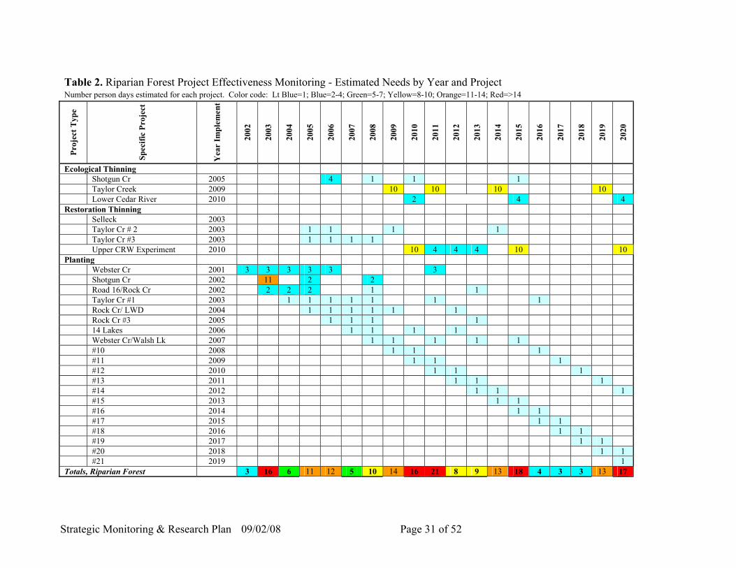
Strategic Monitoring & Research Plan 09/02/08 Page 31 of 52

Table 2. Riparian Forest Project Effectiveness Monitoring - Estimated Needs by Year and Project Number person days estimated for each project. Color code: Lt Blue=1; Blue=2-4; Green=5-7; Yellow=8-10; Orange=11-14; Red=>14

Proj

ect T

ype

Spec

ific

Proj

ect

Yea

r Im

plem

ent

2002

2003

2004

2005

2006

2007

2008

2009

2010

2011

2012

2013

2014

2015

2016

2017

2018

2019

2020

Ecological Thinning Shotgun Cr 2005 4 1 1 1 Taylor Creek 2009 10 10 10 10 Lower Cedar River 2010 2 4 4 Restoration Thinning Selleck 2003 Taylor Cr # 2 2003 1 1 1 1 Taylor Cr #3 2003 1 1 1 1 Upper CRW Experiment 2010 10 4 4 4 10 10 Planting Webster Cr 2001 3 3 3 3 3 3 Shotgun Cr 2002 11 2 2 Road 16/Rock Cr 2002 2 2 2 1 1 Taylor Cr #1 2003 1 1 1 1 1 1 1 Rock Cr/ LWD 2004 1 1 1 1 1 1 Rock Cr #3 2005 1 1 1 1 14 Lakes 2006 1 1 1 1 Webster Cr/Walsh Lk 2007 1 1 1 1 1 #10 2008 1 1 1 #11 2009 1 1 1 #12 2010 1 1 1 #13 2011 1 1 1 #14 2012 1 1 1 #15 2013 1 1 #16 2014 1 1 #17 2015 1 1 #18 2016 1 1 #19 2017 1 1 #20 2018 1 1 #21 2019 1 Totals, Riparian Forest 3 16 6 11 12 5 10 14 16 21 8 9 13 18 4 3 3 13 17

Strategic Monitoring & Research Plan 09/02/08 Page 32 of 52

Table 3. Upland Forest Project Effectiveness Monitoring - Estimated Needs by Year and Project through 2020 Number person days estimated for each project. Color code: Lt Blue=1; Blue=2-4; Green=5-7; Yellow=8-10; Orange=11-14; Red=>14

Proj

ect T

ype

Spec

ific

Proj

ect

Yea

r Im

plem

ent

2002

2003

2004

2005

2006

2007

2008

2009

2010

2011

2012

2013

2014

2015

2016

2017

2018

2019

2020

Ecological Thinning 45 Road 2003 18 15 2 1.5 15 1.5 700 Road 2006 1.5 1.5 18 12 13 9 2 16 2 2 9 16 Barneston 2009 12 12 12 12 Taylor 2010 12 12 12 12 Restoration Thinning Upper Shed 2004 5 15 31 11 5 15 11 5 15 11 Bonus Cr 2002 5 5 5 Taylor Plateau 2006 30 15 15 15 300 Road 2007 30 15 15 15 Planting 45 Road 2004 1 1 1 1 LSPT 2005 1 1 1 1 BPA 2005 1 1 Green Valley 2007 1 1 1 1 #6 2008 1 1 #7 2009 1 1 #8 2010 1 1 #9 2011 1 1 #10 2012 1 1 #11 2013 1 1 #12 2014 1 1 #13 2015 1 1 #14 2016 1 1 #15 2017 1 1 #16 2018 1 1 #17 2019 1 Totals, Upland Forest 7 35 51 33 33 24 74 62 32 34 29 32 27 14 27 17 20 14 14

Strategic Monitoring & Research Plan 09/02/08 Page 33 of 52

Table 4. Long-term Ecological Trend Monitoring Estimated Needs by Year through 2020

Number person days estimated for each project. Color code: Lt Blue=1; Blue=2-4; Green=5-7; Yellow=8-10; Orange=11-14; Red=>14 Pr

ojec

t Typ

e

Spec

ific

Proj

ect

Yea

r In

stal

l

Inst

all N

umbe

r Pl

ots

2003

2004

2005

2006

2007

2008

2009

2010

2011

2012

2013

2014

2015

2016

2017

2018

2019

2020

Upland Forest PSPs Second-growth 2003 17 43 39 4 Second-growth 2004 61 153 35 39 39 39 Old-growth 2003 19 48 Old-growth 2005 18 45 Riparian Forest PSPs Upper Shed 2003 30 75 37 38 Lower Shed 2005 30 75 37 38 Aquatic PMRs PMRs 2005 3 27 PMRs 2006 5 50 . 50 50 50 50 50 PMRs 2006 5 50 50 50 50 50 50 PMRs 2007 5 50 50 50 50 50 50 PMRs 2008 5 50 50 50 50 50 50 PMRs 2009 5 50 50 50 50 50 50 Totals 166 153 147 100 100 100 100 100 100 176 177 176 177 139 100 100 100 100

Strategic Monitoring & Research Plan 09/02/08 Page 34 of 52

Table 5. Estimated Combined Monitoring Needs, Person Days by Year through 2020

Project Type 2002

2003

2004

2005

2006

2007

2008

2009

2010

2011

2012

2013

2014

2015

2016

2017

2018

2019

2020

Upland Ecological Thinning 1.5 20 15 20 0 12 27 33 14 16 2 15 14 12 9 0 18 12 12 Upland Restoration Thinning 5 15 36 11 30 10 45 26 15 15 25 15 11 0 15 15 0 0 0 Upland Planting 0 0 0 2 3 2 2 3 3 3 2 2 2 2 3 2 2 2 2 Riparian Ecological Thinning 0 0 0 0 4 0 1 10 3 10 0 0 10 5 0 0 0 10 4 Riparian Restoration Thinning 0 0 0 2 2 1 1 1 10 4 4 4 1 10 0 0 0 0 10 Riparian Planting 3 16 6 9 6 4 8 3 3 7 4 5 2 3 4 3 3 3 3 LWD Placement 12 8 8 35 9 12 4 8 7 2 3 4 7 10 3 6 5 6 7 Streambank Stabilization 12 8 16 11 6 2 4 4 8 6 6 6 6 10 8 8 8 8 8 Planting 0 0 0 0 0 0 1 2 2 2 2 1 1 1 0 0 0 0 0 Upland Forest PSPs 0 91 153 45 0 0 0 0 0 0 39 39 39 39 39 0 0 0 0 Riparian Forest PSPs 0 75 0 75 0 0 0 0 0 0 37 38 37 38 0 0 0 0 0 Aquatic PMRs 0 0 0 27 100 100 100 100 100 100 100 100 100 100 100 100 100 100 100Total 34 233 234 237 160 143 193 190 165 165 224 229 230 230 181 134 136 141 146

Strategic Monitoring & Research Plan 09/02/08 Page 35 of 52

Table 6. HCP-defined monitoring categories and subcategories and the responsible team or work group.

Monitoring Category

Project Type Project Category Responsible ID Team or Work Group

Upland and Riparian Forests

Forest Ecology and Fish & Wildlife Work Groups

Aquatic Habitats Hydrology and Fish & Wildlife Work Groups

Long-term Ecological Trends

Integration of Watershed Processes

Water Quality All Restoration ID Teams; Hydrology, Fish & Wildlife, and Forest Ecology Work Groups

Ecological Thinning Upland Forest Restoration ID Team; Project Teams Restoration Thinning Upland Forest Restoration ID Team; Project Teams

Upland Forest Habitat Restoration

Upland Planting Upland Forest Restoration ID Team; Project Teams Conifer Underplanting Riparian Restoration ID Team; Project Teams Restoration Thinning Riparian Restoration ID Team; Project Teams

Riparian Forest Habitat Restoration

Ecological Thinning Riparian Restoration ID Team; Project Teams Streambank Stabilization Aquatic Restoration ID Team; Project Teams Streamside Re-vegetation Aquatic Restoration ID Team; Project Teams

Aquatic Habitat Restoration

LWD Placement Aquatic Restoration ID Team; Project Teams Stream Crossings Project Teams; Hydrology and Fish & Wildlife Work Groups Road Decommissioning Project Teams; Hydrology Work Group

Restoration Projects

Roads

Road Improvement, Stabilization, Repair, Maintenance

Aquatic Restoration ID Team; Hydrology Work Group

Upland Species Fish & Wildlife Work Group Aquatic Species Fish & Wildlife and Hydrology Work Groups Anadromous Fish Passage Fish Ladder Counts

Science and Technical Services Division

Anadromous Fish Passage Habitat Use & Distribution

Science and Technical Services Division; Fish & Wildlife Work Group; collaborating with UW researchers and state and federal agencies

Species Specific

Optional Species Fish &Wildlife Work Group

Strategic Monitoring & Research Plan 09/02/08 Page 36 of 52

Table 7. Monitoring needs not specifically addressed in the HCP. Monitoring Need Justification Responsible Group

Threats - Number and distribution of invasive, non-native species (plant and animal) in CRMW, and effectiveness of control methods

High risk of negative ecological consequences of invasive species, especially in wetlands. The legal (state) requirement to monitor and control certain invasive plants.

Invasive Species ID Team

Changes in populations of cutthroat trout, kokanee, or other species of fish in the CRMW

Ecological response to reintroduction of anadromous fish to CRMW.

Fish & Wildlife Work Group

Baseline information and trends in biodiversity in CRMW (could include insects, amphibians, cryptogams, etc.)

The HCP commitment to protect and restore biodiversity.

Biodiversity Project Team; All Ecosystem Work Groups

Condition and extent of special habitats (e.g., changing plant communities)

The HCP commitment to protect and restore biodiversity.

All Ecosystem Work Groups, likely collaborating with UW researchers

Changes in plant communities as a result of climate change

The need to plan for expected future change to meet the HCP commitments to accelerate late-successional forest development. The HCP commitment to protect and restore biodiversity.

All Ecosystem Work Groups, Outside agencies, UW researchers

Reproductive success of common loons in the Tolt Reservoir

Responsible management related to reservoir operation.

Fish & Wildlife Work Group

Number and distribution of invasive, non-native species (plant and animal) in the Seattle ownership in the Tolt watershed and the Lake Youngs Reservation, and effectiveness of methods for control

High risk of negative ecological consequences of invasive species, especially in wetlands. The legal (state) requirement to monitor and control certain weeds.

Invasive Species ID Team

Contaminant levels, acidification in streams in upper watershed due to atmospheric deposition

Potential ecological consequences on biodiversity (especially insects and amphibians). Potential municipal water quality issues.

Hydrology Work Group, Watershed Protection, Outside agencies, UW researchers

Size, composition of ungulate and large carnivore populations

Required for responsible ecosystem management and the Settlement Agreement with the Muckleshoot Indian Tribe

Fish & Wildlife Work Group, Outside agencies, Muckleshoot Indian Tribe, Other Tribes

6.0 PRIORITIZATION OF MONITORING EFFORTS The need for monitoring is far greater than available funding, necessitating prioritization to ensure the most essential data are collected. All four major monitoring components (species-specific, threats, long-term ecological trend, and project-specific monitoring - see Figure 2) require some level of monitoring effort. Consequently, each component will be prioritized separately. Additionally, within project monitoring, the different types of restoration projects (upland, riparian, aquatic, and roads) all require monitoring and will also be prioritized separately. The upland forest, riparian forest, and aquatic restoration ID teams will develop big-picture programmatic monitoring strategies for their program areas. The Monitoring ID team

Strategic Monitoring & Research Plan 09/02/08 Page 37 of 52

will oversee and review this process, and make recommendations as needed. Monitoring municipal water quality will continue to be conducted by the Utility Systems Management Branch, and will not be considered here. Water quality monitoring to address ecological processes will be integrated into long-term ecological and project monitoring. Prioritizing monitoring is contingent on knowing the amount of available funding. Limited directed monitoring funding is provided by the HCP (see section 7), and attempting to prioritize among projects prior to knowledge about the level of funding available will be difficult. The Monitoring and Research ID Team can assist in the prioritization effort by reviewing monitoring plans, examining budget shortfalls, and exploring the possibilities of coordination and integration of data collection among projects that could help close the shortfalls. 6.1 Prioritization of Species Monitoring The minimum amount of species-specific monitoring is clearly dictated in the HCP, with associated funding provided by year. These monitoring projects will be administered by the appropriate work groups (Table 5). Additional species monitoring will be prioritized by the appropriate work groups after evaluating the level of uncertainty, the management utility, monitoring costs, and potential funding. Some species monitoring may be conducted in conjunction with other agencies or as part of cooperative research projects. 6.2 Prioritization of Threat Monitoring There are three primary threats to ecological processes, functions, and wildlife habitat under HCP management guidelines: fire, climate change, and invasive species. Large-scale fire is a significant risk to the entire watershed and specifically to municipal water quality. Consequently, during high-risk times of the year, standard fire monitoring protocols are the highest priority and are used by all staff and contractors. Vulnerability to fire is addressed in the Synthesis Framework document (Erckmann et al. 2008) and is being evaluated and prioritized by the Forest Ecology work group. Climate change is potentially a risk to critical habitats in the future. However, it is expected to result in relatively slow changes, and thus is a lower priority. Plant responses to climate change in forests will be monitored using data from the long-term ecological trend plots. Other types of monitoring, such as invasion of trees or non-native plants into meadows, will be planned in 2008-2009. Invasive species are a primary on-going threat to watershed functioning. It is critical to ensure early detection of new invasive species when control and eradication are still possible for a relatively small outlay of resources. There will be intensive survey efforts in 2007 and 2008 to discover and document all legally-required and selected other noxious weed species in all habitats at high risk of invasion in the CRMW, the Tolt Municipal Watershed, and the Lake Youngs Reserve. This includes areas with high available light or frequent disturbance, such as wetlands, meadows, road corridors, and riparian areas. Heavily forested areas will not be surveyed because of the lower likelihood of invasives species occurring in that habitat. Monitoring for currently known and potential new invading species is a high priority and will be conducted annually starting in 2009 in key areas identified during the intensive surveys. This will likely incorporate a rotating panel design, where a percentage (e.g., 20%) of the area is surveyed each year, repeating the entire panel every five years. In addition, data from the long-

Strategic Monitoring & Research Plan 09/02/08 Page 38 of 52

term ecological trend plots (upland and riparian forest PSPs) will be used to document invasive plant species throughout the watershed. 6.3 Prioritization of Long-term Ecological Trend Monitoring Plot establishment and baseline sampling for all types of long-term ecological trend monitoring (aquatic, riparian, and upland forest) will be completed by 2009. Data from future measurements of these permanent plots may reveal numerous insights that will influence future management decisions, including unexpected developmental trajectories, areas that no longer require restoration intervention, or unanticipated threats to critical ecological processes and functions. Repeat measurements will be prioritized within each monitoring type, and will be staggered such that the highest priority plots will be sampled earliest. Priorities may change in response to future conditions or management priorities, but highest priority plots are expected to include those in areas of high natural or man-made disturbance, sites with rapid vegetation growth, and areas near ecotones. 6.4 Prioritization of Project Effectiveness Monitoring All restoration project types (aquatic, riparian, upland, and roads) must be monitored, so prioritization will primarily take place within, rather than among project types. When project teams are deciding whether and how much to monitor, they should follow the process illustrated in Figure 4. The criteria they should consider, listed in order of their relative importance, are: 1. Level of Risk of Adverse Environmental Impact. If a restoration technique has a high risk

of adverse environmental impact, but benefits of the project are judged to outweigh the risks, then monitoring must be employed to provide the opportunity to quickly mitigate if an adverse impact is detected. Highest priority will be given to projects that pose a risk to water quality, because of the primary function of the CRMW as a municipal water supply. Projects that could potentially affect water quality will usually be those that involve manipulations of in-stream or channel bank structures and road projects. Consequently, it will be aquatic, roads, and perhaps riparian restoration projects that may need to monitor water quality.

2. Level of Uncertainty About Restoration Technique or Outcome. If uncertainty about the

outcome of a restoration technique or other management action is high, then monitoring is a high priority. Generally an active adaptive management strategy should be employed when possible so that lessons learned can be applied more widely to future projects (see section 2).

3. Level of Management Utility. Asset management principles dictate that data from

monitoring funded by SPU support future management decisions. Management utility as used here includes two primary components. First, the same or similar restoration technique will be repeated several times, so information provided will directly influence whether the technique will be repeated unchanged or modified. Second, at least some of the variables measured must respond to the treatment in a short enough time frame that results can be evaluated and used in designing future projects.

4. Amount of Area Affected. Projects impacting large areas entail a higher risk of long-lasting

ecological consequences than those affecting small areas, and thus are a higher monitoring priority (e.g., restoration thinning >10,000 acres versus ecological thinning 2,000 acres).

Strategic Monitoring & Research Plan 09/02/08 Page 39 of 52

5. Project Cost. If the above factors are equivalent, projects that are expensive to plan and

implement (e.g., a road decommissioning project in an ecologically sensitive site) are more important to monitor than less expensive projects, because of the financial risk involved.

6. Monitoring Cost. Finally, if all other factors are equal, monitoring cost will drive the

decision. Priority will be given to projects that have lower data collection costs. The greatest cost efficiency will be achieved in situations that will yield high benefits, in terms of management information gained, for relatively low data collection cost. A simple example of high “bang for the buck” would be the relative survival of different species of trees planted in a riparian zone. Simply monitoring the survival rate by species has high management utility, but is low cost to achieve. Documenting seedling growth and vigor, along with key environmental variables will yield greater management and scientific benefits, but also entail greater costs.

If using the above procedure results in multiple projects at the same level of monitoring priority, then additional criteria should be considered. The Synthesis Framework Document (Erckmann et al. 2008) delineates synergy areas where restoration projects should produce the greatest environmental benefits for the largest number of species. Focusing monitoring in these areas should provide greater coordination and integration of data collection efforts, as well as information used to evaluate the synergistic effects. Finally, because contributing to scientific knowledge is a Watershed Services Division goal, if monitoring data from certain projects will further the science of restoration more than other projects, they will be a higher priority.

Strategic Monitoring & Research Plan 09/02/08 Page 40 of 52

High Risk of Adverse Environmental Impact

(including water quality)?

YesHigh

Monitoring Priority

No

High Uncertainty about Outcome?

No High Management Utility?

No MonitoringNo

Yes

Large Area Affected? No High Project Cost?

Yes

Moderate Monitoring

Priority

No

Yes

Moderate Monitoring

PriorityHigh Monitoring Cost?

Yes

No Monitoring

No

Low Monitoring

Priority

Yes

Figure 4. Prioritization process for restoration project monitoring. 7.0 FUNDING 7.1 HCP Compliance In most cases, compliance in the HCP was identified as a monetary commitment, although for many restoration projects cost per acre was estimated and approximate number of treated acres by project type was calculated. The City will be held only to the cost commitment, however, not

Strategic Monitoring & Research Plan 09/02/08 Page 41 of 52

to the estimated number of acres, with the exception of the commitment to decommission 236 miles of road. 7.2 Budgets and Funding Gaps Although compliance and effectiveness monitoring in an adaptive management context is mandated in the HCP, the budget dedicated to monitoring was extremely limited. Some Operations and Maintenance (O&M) budgets are provided to address tracking long-term habitat trends, limited species monitoring, and fish ladder counts and water quality measurements associated with anadromous fish passage at Landsburg. Plus some of the research projects described in section 2.3 are funded. In addition, other O&M budgets have been used for baseline data collection and may be available for monitoring in the future. Numerous funding gaps exist, however. A critical need that has no dedicated funding is to monitor the ecological consequences of road decommissioning and improvement. Another critical need is the HCP commitment to protect and restore biodiversity, implying a need to identify elements of biodiversity, evaluate the condition of those elements, and track their condition over time. The framework for biodiversity monitoring was established with the upland and riparian forest PSPs and PMRs. However, there is a future funding need to resample these permanent plots, as well as repeat remotely-sensed image data. Funding was not provided for monitoring habitat use and distribution of anadromous fish associated with fish passage at Landsburg. There is also a funding gap to monitor evidence of how global climate change is affecting the biodiverisity, and key ecological processes and functions in the watershed. Monitoring invasive species is a key component of this, as they are predicted to increase under probable climate change scenarios. Finally, there is a funding gap for data management and analysis. Time and resources devoted to data entry, management, and analysis can equal or exceed that involved in field collection of data (Gibbs et al. 1999). Issues of reporting, sharing, and archiving data are also critical. Because the value of monitoring data increases substantially with time, it is essential that there is adequate funding for data documentation and maintenance. 7.3 Funding Options Because effectiveness monitoring and adaptive management is mandated in the HCP and is essential for future management decisions, we recommend that the project ID teams, other project groups, and appropriate work groups explicitly dedicate a percentage of the total Capital Improvement Project (CIP) budget to collecting baseline and immediate post-project data. The percentage will vary depending on the fixed costs of the project, key questions, hypotheses, sampling design, and intensity, duration, and spatial extent of data collection required to answer the questions. The amount of project budget dedicated to monitoring should be addressed in the individual monitoring strategies and plans. Monitoring must continue long past project completion, when CIP project budgets typically are closed, however. Consequently, longer-term monitoring must be funded by other sources, such as O&M funds. However, these types of funds are typically very difficult to obtain. So a policy decision on O&M funding for effectiveness and adaptive management monitoring needs to occur. The Monitoring and Research ID Team will work with the restoration ID teams to attempt to smooth out the data collection effort over all projects over the years, to make O&M allocation more practical.

Strategic Monitoring & Research Plan 09/02/08 Page 42 of 52

Assigning a percentage of the total project budget funding may be insufficient to address all monitoring key questions. An additional option would be to pool funds across several HCP budgets to address a coordinated series of projects and other needs, which may be the most efficient solution for some adaptive management needs. Other options to supplement monitoring budgets include establishing collaborative projects or creating cost shares with universities, agencies, or individuals, utilizing grant opportunities, using interns and volunteers to help collect data, and utilizing excess revenues (if any) generated from ecological thinning. Professional grant writers may be needed to assist in obtaining adequate funding for monitoring. 8.0 ONGOING OVERSIGHT AND COORDINATION Since resources, evaluation methodologies, and budgets change with time, and restoration projects have varying start times, ongoing oversight and support by the Monitoring and Research ID Team will help to ensure coordination, integration, and cost effectiveness of monitoring efforts. Team members are expected to change over time, serving on a rotational basis to provide overlap, ensure continuity, and maintain good transition of membership. The Monitoring and Research ID Team will help to track and coordinate the monitoring efforts by the various ID teams, project teams, and work groups. They will meet at least once annually to review all monitoring completed in the previous field season and planned for the upcoming season. They will manage the overall monitoring tracking database, and can function as a reminder for scheduled monitoring to occur at the appropriate interval. They can also review associated costs and funding levels by year and identify any coordination of data collection among projects that could result in cost savings. If funding does not permit all data collection scheduled for a particular year, they will be available to make recommendations on prioritization. All project teams and work groups that are conducting monitoring activities will be responsible for communicating plans and schedules to the Monitoring and Research ID Team. 8.1 Monitoring Strategy and Plan Review The primary monitoring strategies, including identification of key risks, uncertainties, and threats, will be included in the monitoring sections of the restoration strategic plans, with detailed monitoring plans in individual restoration project plans. If needed, the Monitoring and Research ID Team will be available to provide support and consultation to other teams during monitoring strategy and plan development. It will be the Monitoring and Research ID Team’s responsibility to ensure that monitoring plans follow the recommended standards and guidelines and that other recommendations put forth in this document are considered. 8.2 Information Exchange The Monitoring and Research ID Team will act as a communication hub and liaison among other ID and project teams by providing coordination and information about ongoing and upcoming monitoring. This will be accomplished by developing and maintaining the monitoring tracking database (described in section 5.3) and coordinating periodic monitoring notices or presentations. The Monitoring and Research ID Team lead will ensure that all projects are entered into the monitoring database. Because data collected by ID and Project Teams will be collected in a manner consistent with data documentation and management guidelines, support from the Information Technology workgroup will facilitate this process. Support in problem solving and

Strategic Monitoring & Research Plan 09/02/08 Page 43 of 52

assistance in obtaining appropriate experts, statisticians, and other professionals will be provided, as needed. 8.3 Future Changes/Adaptive Management As results are generated, data may indicate that some restoration activities are not effective in achieving the stated goals and objectives. The Monitoring and Research ID Team, along with other ID and project teams, will be available to periodically review the monitoring data to determine whether recommendations for changes in prescriptions should be made. Also periodic reviews of results and new monitoring techniques from outside the watershed will be made to ensure the latest information is being included in the monitoring efforts. 9.0 RECOMMENDATIONS AND NEXT STEPS This plan will be used by Watershed Services Division staff to guide monitoring and research in the CRMW. The plan will be reviewed and potentially updated every five years (more often, if needed), to ensure it is still current and applicable, and to incorporate any new findings from the literature. Database and Monitoring Strategy Development We expect to complete the Project Tracking Database by early spring, 2008. This will then be used as the basis for developing the Monitoring Tracking Database, which is anticipated to be completed by fall, 2008. The Monitoring Location GIS map will be created subsequent to this, as time and funding allows. The ID team members will maintain and update the databases annually, as projects are planned and implemented. In addition to developing these databases, we will work with restoration ID teams in 2008 on the development of the programmatic monitoring strategies, continuing the effort started in 2007. Science Information Quality System Once the SIQS is finalized, it will be reviewed by the Monitoring and Research ID team. If any elements of the SIQS are not present in this plan, they will be incorporated at that time. The Monitoring and Research ID team will ensure that all monitoring plans will include all the elements of the SIQS. Invasive Species A CIP project to develop an Invasive Species Program for the CRMW, the Tolt Municipal Watershed, and the Lake Youngs Reserve was initiated in 2007. By the end of 2008, botanists will have surveyed all high-risk habitats for all invasive species that we are legally required to control. In addition, a large number of control efforts will have been implemented and data collected, both on legally required species and on species that cause significant ecological damage, but are not legally required to control. CIP funding is anticipated to continue only through 2008, with O&M funding for the program in 2009 and beyond uncertain. We recommend that, at a bare minimum, a program to continue control of all legally required species, and selected species of known high ecological risk (e.g., knotweed) be funded with on-going O&M funding. In addition, we recommend including an early detection/rapid response protocol in which annual surveys in a rotating panel design be conducted for new infestations.

Strategic Monitoring & Research Plan 09/02/08 Page 44 of 52

This allows a cost-effective way to monitor and treat new infestations while they are still small and easily eradicated. Water Quality as an Integrator of Ecosystem Processes We recommend that staff investigate the idea of incorporating water quality monitoring as means to integrate physical and biological processes in subbasins. These discussions should occur between the Monitoring and Research ID team and the restoration ID teams. Part of this would likely include field checking sediment model results to ensure that the models are accurately predicting sediment changes from road improvement and decommissioning projects. But there should also be consideration of whether it would make sense to monitor key water quality indicators in basins with large amounts of upland, riparian, and aquatic restoration projects. Currently a water quality monitoring plan in relation to salmon passing through the Landsburg fish ladder is being developed by non-watershed SPU staff, so will not be addressed in this plan. Long-term Trend Monitoring – Remotely Sensed Data Repeating remotely sensed data collection at intervals in the future is critical to documenting how the entire watershed is changing through time. This would potentially include aerial photographs, Master data, and Lidar data, including canopy height. These types of data would likely be collected, analyzed, and funded in coordination with other agencies such as King County and the University of Washington, and potentially utilizing grant funding. Climate Change The effects of global climate change are becoming a major issue for SPU, not only concerning future water supply, but also for habitat for federally listed species. We recommend that during 2008 staff develop a plan to monitor key habitats for response to climate change. This should include monitoring selected alpine meadows to track tree invasion, invasion by non-native plants, and change in native plant composition. It should also include monitoring some wetlands for response to climate change. Data collection could focus on changes in hydrology, native plant species composition, invasive plant species, and potentially use by key animal species such as amphibians. Funding for these types of efforts has not yet been addressed, but there may be some options during the 2009-2010 budget planning process. Funding In order for adaptive management to be effective, monitoring data must be collected and analyzed to provide information for future decisions. Consequently, it is critical to address the funding shortfalls identified in Section 7. Some funding for program and project monitoring does exist, but increased O&M funds will be required over the next 8 to10 years to adequately address the uncertainties inherent in restoration activities. The Monitoring and Research ID team will work with the restoration ID teams in early 2008 to develop a rotating panel design for all monitoring data collection to smooth out work load over the years. This should help in predicting staff work load and in obtaining new O&M funding for monitoring, because O&M funds are consistent between years. A design that involved highly pulsed data collection, with large amounts in some years and none in others, would be much more difficult to fund.

Strategic Monitoring & Research Plan 09/02/08 Page 45 of 52

In addition, ID team members will be available to work with the HCP Oversight Committee, as needed, to obtain funding from grants or other sources for anadromous fish monitoring, both below and above the Landsburg Diversion Dam. 10.0 REFERENCES Ahlstrand, G., J. Hadfield, R. Holmes, J. Kailin, P Reeberg, E. Schreiner. 2001. Long-Term

Ecological Monitoring Conceptual Plan for Terrestrial Vegetation. In: B. Freet. North Cascades National Park Service Complex Long-Term Ecological Monitoring Conceptual Plan. Available online at: http://www.nps.gov/noca/Ltem/index.htm.

Anderson, D.R., K.P. Burnham, and W.L. Thompson. 2000. Null hypothesis testing: problems,

prevalence, and an alternative. Journal of Wildlife Management 64:912-923. Aubry, K.B. 2000. Amphibians in managed, second-growth Douglas-fir forests. Journal of

Wildlife Management 64:1041-1052. Aubry, K.B., F.G. Hallett, S.D. West, M.A. O’Connell, and D.A. Manuwal. 1997. Wildlife use

of managed forests: a landscape perspective. Timber, Fish and Wildlife Publication TFW-WL4-98.

Bartels, R., J.D. Dell, R.L. Knight, and G. Schaefer. 1985. Dead and down woody material. In:

E.R. Brown (ed), Management of Wildlife and Fish Habitats in Forests of Western Oregon and Washington. USDA Forest Service R6-F&WL-192.

Beach, E.W. 2003. Regional riparian management cooperative prospectus. Unpublished

document, Center for Streamside Studies, University of Washington, Seattle. Beechie, T.J., C.N. Veldhuisen, D.E. Schuett-Hames, P. DeVries, R.H. Conrad, and E.M.

Beamer. (draft). Monitoring actions to reduce sediment from unpaved roads. Proposed book chapter, 123 pp.

Bilby, R. E. B. R. Fransen, and P. A. Bisson. 1996. Incorporation of nitrogen and carbon from

spawning coho salmon into the trophic system of small streams: evidence from stable isotopes. Canadian Journal of Fisheries and Aquatic Sciences 53: 164-173.

Black, R.W. and D.E. MacCoy. 1999. The development and evaluation of a benthic index of

biological integrity for the Cedar River watershed, Washington. U.S. Geological Survey, Water-Resources Investigations Report 99-4203.

Bohle, T., D. Beedle, H. Barnett, M. Joselyn, and A. LaBarge. 2008. Aquatic Restoration

Strategic Plan. Ecosystem Section, Watershed Services Division, Seattle Public Utilities. Burnham, K.P. and D.R. Anderson. 2002. Model selection and multimodel inference: a practical

information-theoretic approach. Springer-Verlag, New York, New York. 488 pp.

Strategic Monitoring & Research Plan 09/02/08 Page 46 of 52

Busch, D.E. and J.C. Trexler. 2003. Monitoring Ecosystems, Interdisciplinary Approaches for

Evaluating Ecoregional Initiatives. Island press. Washington DC. Carey, A.B. and S.M. Wilson. 2001. Induced spatial heterogeneity in forest canopies: responses

of small mammals. Journal of Wildlife Management 65:1014-1027. Cedar River Watershed Habitat Conservation Plan. 2000. Available for review from Seattle

Public Utilities. http://www.seattle.gov/util/About_SPU/Water_System/Habitat_Conservation_Plan--HCP/index.asp

Chapin, D., T. Bohle, M. Borsting, M. Joselyn, A. LaBarge. 2008. Riparian Restoration Strategic

Plan. Ecosystem Section, Watershed Services Division, Seattle Public Utilities. DeAngelis, D.L., L.J. Gross, E.J. Comiskey, W.M. Mooij, M.P. Nott, and S. Bellmund. 2003.

The use of models for a multiscaled ecological monitoring system. In: Monitoring Ecosystems, Interdisciplinary Approaches for Evaluating Ecoregional Initiatives. D.E. Busch and J.C. Trexler (eds). Island press. Washington DC.

Dixon, P.M., A.R. Olsen, and B.M. Kahn. 1998. Measuring trends in ecological resources.

Ecological Applications 8:225-227. Dubé, K., W. Megahan, and M. McCalmon, 2004. Washington road surface erosion model

(WARSEM). Unpublished report prepared for the State of Washington Department of Natural Resources. February 20, 2004. Available to download at: http://www.dnr.wa.gov/forestpractices/adaptivemanagement/cmer/warsem/

Dyrland, D. and others. 1993. Forest monitoring and evaluation guide, region 6. USDA Forest

Service Report. Dyrness C. T. and S.A. Acker. 1999. Reference Stands in or near the H.J. Andrews Experimental

Forest. Permanent Plots of the Pacific Northwest. Report Number 2. (http://www.fsl.orst.edu/lter/pubs/webdocs/permplot.cfm)

Dyrness, T. and S. Acker. 2000. Permanent plots in Mount Rainier National Park. Permanent

Plots in the Mount Rainier National Park. Permanent Plots of the Pacific Northwest. Report Number 4. (http://www.fsl.orst.edu/lter/pubs/webdocs/permplot.htm)

Eagle, P. and S. Droege. 1999. Power Analysis of Monitoring Programs. Patuxent Wildlife

Research Center. Available online at: http://www.mp1-pwrc.usgs.gov/powcase/index.html.

Eagle, P., J. P. Gibbs, And S. Droege. 1999. Power Analysis of Wildlife Monitoring Programs:

Exploring the Trade-Offs Between Survey Design Variables and Sample Size

Strategic Monitoring & Research Plan 09/02/08 Page 47 of 52

Requirements. Patuxent Wildlife Research Center. Available online at: http://www.pwrc.usgs.gov/resshow/droege3rs/salpower.htm.

Elzinga, C.L., D.W. Salzer, and J.W. Willoughby. 1998. Measuring and Monitoring Plant

Populations. Bureau of Land Management Technical Reference 1730-1, BLM/RS/ST-98/005+1730.

Erckmann, D. Beedle, J. T. Bohle, M. Borsting, D. Chapin, A. LaBarge,, D. Munro, S.

Nickelson, D. Paige 2008. A Synthesis Framework for the Cedar River Watershed Habitat Conservation Plan. Ecosystem Section, Watershed Services Division, Seattle Public Utilities.

Erickson, J. 1997. Managed forests in the western Cascades: the effects of seral stage and

landscape structure on bat habitat use patterns. In: Aubry, K.B., J.G. Hallett, S.D. West, M.A. O’Connell, and D.A. Manuwal, eds. Wildlife use of managed forests: a landscape perspective. Timber, Fish and Wildlife Report TFW-WL4-98-002.

Fancy, S. 2000. Guidance for the Design of Sampling Schemes for Inventory and Monitoring of

Biological Resources in National Parks. Available online at: http://www.nature.nps.gov/im/monitor/nps_sg.doc

Franklin, J.F., K. Cromack, W. Denison, A. McKee, C. Maser, J. Sedell, F. Swanson, and G.

Juday. 1981. Ecological characteristics of old-growth Douglas-fir forests. USDA Forest Service General Technical Report PNW-118.

Freet, B., 2001. North Cascades National Park Service Complex Long-Term Ecological

Monitoring Conceptual Plan. Available online at: http://www.nps.gov/noca/Ltem/index.htm.

Gates, D. M. 1993. Climate Change and its Biological Consequences. Sinauer, Sunderland, MA. Gibbs, J.P., H.L. Snell, and C.E. Causton. 1999. Effective monitoring for adaptive wildlife

management: lessons from the Galapagos Islands. Journal of Wildlife Management 63: 1055-1065.

Grant, W.E., E.K. Pederson, and S.L. Marin. 1997. Ecology and Natural Resource Management

Systems Analysis and Simulation. John Wiley & Sons. New York. Gunderson, L.H. 2003. Learning to monitor or monitoring to learn? In: Busch, D.E. and J.C.

Trexler (eds). Monitoring Ecosystems, Interdisciplinary Approaches for Evaluating Ecoregional Initiatives. Island press. Washington DC.

Hankin, D.G., and G.H. Reeves. 1988. Estimating total fish abundance and total habitat area in

small streams based on visual estimation methods. Canadian Journal of Fisheries and Aquatic Sciences 45:834-844.

Strategic Monitoring & Research Plan 09/02/08 Page 48 of 52

Hagar, J.C., W.C. McComb, and W.H. Emmingham. 1996. Bird communities in commercially

thinned and unthinned Douglas-fir stands of western Oregon. Wildlife Society Bulletin 24:353-366.

Haveri, B.A. and A.B. Carey. 2000. Forest management strategy, spatial heterogeneity, and

winter birds in Washington. Wildlife Society Bulletin 28:643-652. Hemstrom, M.; Spies, T.A.; Palmer, C.J.; Kiester, R.; Teply, J.; McDonald, P.; and Warbington,

R. 1998. Late-successional and old-growth forest effectiveness monitoring plan for the Northwest Forest Plan. Gen. Tech. Rep. PNW-GTR-438. Portland, OR: U.S. Department of Agriculture, Forest Service, Pacific Northwest Research Station. 37 p.

Henderson, J.A., D.H. Peter, R.D. Lesher, and D.C. Shaw. 1989. Forested plant associations of

the Olympic National Forest. USDA Forest Service Pacific Northwest Region. R6 Ecol Technical Paper 001-88.

Henderson, J. and R. Lesher. 2002. Survey Protocols for benchmark plots (permanent intensive

ecopolots) for western Washington, version 1.22. U.S. Forest Service Pacific Northwest Region unpublished report.

Holling, C. S. 1978. Adaptive environmental assessment and management. John Wiley, New

York, New York, USA. Humes, M.L., J.P. Hayes, and M.W. Collopy. 1999. Bat activity in thinned, unthinned, and old-

growth forests in western Oregon. Journal of Wildlife Management 63:553-561. Iles, K. 2002. Seattle Watershed Inventory. Unpublished report to Seattle Public Utilities.

Available for review from Seattle Public Utilities, Watershed Management Division. Jenkins, K. A. Woodward, and E. Schreiner. 2002. A Framework for Long-term Ecological

Monitoring in Olympic National Park: Prototype for the Coniferous Forest Biome. USGS Forest and Rangeland Ecosystem Science Center. Available online at: http://fresc.usgs.gov/olympic/research/framework.pdf

Jenny, H. 1941. Factors of Soil Formation. McGraw-Hill, New York. Johnson, B. L. 1999. The role of adaptive management as an operational approach for resource

management agencies. Conservation Ecology 3(2): 8. Johnson, D.H. and T.A. O’Neil. 2001. Wildlife-habitat relationships in Oregon and Washington.

Oregon State University Press. Corvallis, OR.

Strategic Monitoring & Research Plan 09/02/08 Page 49 of 52

Johnson, M.D. 1998. Region 6 Inventory and Monitoring System. Field procedures for the Current Vegetation Survey. USDA Forest Service, Pacific Northwest Region. Portland, OR.

Kershner, J.L., M. Coles-Ritchie, E. Cowley, R. C. Henderson, K. Kratz, C. Quimby, D. M.

Turner, L. C. Ulmer, and M. R. Vinson. 2001. A Plan to Monitor the Aquatic and Riparian Resources in the Area of PACFISH/INFISH and the Biological Opinions for Bull Trout , Salmon, and Steelhead. USDA Forest Service Effectiveness Monitoring Module- PIBO Monitoring Plan.

Kiffney, P., C. Volk, J. Hall, and C. Eberhart. 2002. Community and ecosystem attributes of the

Cedar River watershed above Landsburg Diversion before arrival of Pacific salmon. Unpublished report to Seattle Public Utilities. Available for review from Seattle Public Utilities, Watershed Management Division.

LaBarge, A, R. Gersonde, S. Nickelson, B. Richards, D. Munro, C. Antieau. 2008. Upland

Forest Habitat Restoration Strategic Plan. Ecosystem Section, Watershed Services Division, Seattle Public Utilities.

Lee, K.N. 1993. Compass and Gyroscope: Integrating Science and Politics for the Environment.

Island Press, Washington DC. Lofroth, E.C. 1998. The dead wood cycle. In: Voller, J., and S. Harrison (eds), Conservation

Biology Principles for Forested Landscapes. Vancouver, BC: University of British Columbia Press.

Manuwal, D. and S. Pearson. 1997. Bird populations in managed forests in the western Cascade

Mountains, Washington. In: Aubry, K.B., J.G. Hallett, S.D. West, M.A. O’Connell, and D.A. Manuwal, eds. Wildlife use of managed forests: a landscape perspective. Timber, Fish and Wildlife Report TFW-WL4-98-002.

Margoluis, R. and N. Salafsky. 1998. Measures of success: designing, managing and monitoring

conservation and development projects. Island Press, Washington D.C. Marmorek, D. 2003. What is adaptive management? Presented in: Making it work: strategies for

effective adaptive management workshop. City of Seattle and Washington Trout. Max, T.A., H.T. Schreuder, J.W. Hazard, D.D. Oswalk, J. Teply and J. Alegria. 1996. The

pacific northwest region vegetation and inventory monitoring system. USDA Forest Service, Pacific Northwest Research Station. PNW-RP-493.

McConnell, R.L., and D.C. Abel. 2002. Environmental issues: measuring, analyzing and

evaluating. Upper Saddle River, New Jersey: Prentice Hall. McDonald, T. L. (2003). “Review of environmental monitoring methods: survey designs,”

Environmental Monitoring and Assessment, 85, 277-292.

Strategic Monitoring & Research Plan 09/02/08 Page 50 of 52

Mollot, L. 2005. The Use of Remote Sensing, GIS, and Multivariate Vegetation Analysis to

Explain the Distribution of Riparian Plant Communities at Multiple Spatial Scales. Ph.D Dissertation. University of Washington.

Montgomery, D.R. and J.M. Buffington. (1997). “Channel Reach Morphology in Mountain

Drainage Basins,” Geological Society of America Bulletin, 109, 596-611. Moss, D., M.T. Furse, J.F. Wright, and P.D. Armitage. 1987. The prediction of the macro

invertebrate fauna of unpolluted running-water site in Great Britain using environmental data. Freshwater Biology 17:41-52.

Mulder, B.S.; Noon, B.R.; Spies, T.A.; Raphael, M.G.; Palmer, C.J.; Olsen, A.R.; Reeves, G.H.;

and Welsh, H.H (tech coor). 1999. The strategy and design of the effectiveness monitoring plan for the Northwest Forest Plan. Gen. Tech. Rep. PNW-GTR-437. Portland, OR: U.S. Department of Agriculture, Forest Service, Pacific Northwest Research Station.

Munro, D., S. Nickelson, D. Chapin, M. Joselyn, B. Lackey, D. Paige, D. Beedle, L.

Boeckstiegel, W. Sammarco, and C. Anderson. 2003. A Proposal for the Establishment of Permanent Sample Plots in the Cedar River Municipal Watershed. Cedar River Watershed unpublished report.

Murray, C.L., D.R. Marmorek and W.A. Kurz. 2000. De-mystifying Adaptive Management -

Instructor’s Manual. Revised Edition. Prepared by ESSA Technologies Ltd., Vancouver, BC for BC Forest Service, Victoria, BC, 98 pp. + appendices.

National Science and Technology Council. 1997. Integrating the nation’s environmental

monitoring and research networks and programs: a proposed framework. Office of the White House, Washington, D.C.: The Environmental Monitoring Team of the Coommittee on Environment and Natural Resources, Office of the White House, Washington, D.C.

Noon, B.R., T.A. Spies, and M.G. Raphael. 1999. Conceptual basis for designing an

effectiveness monitoring program. In: Mulder, B.S.; Noon, B.R.; Spies, T.A.; Raphael, M.G.; Palmer, C.J.; Olsen, A.R.; Reeves, G.H.; and Welsh, H.H (tech coor). 1999. The strategy and design of the effectiveness monitoring plan for the Northwest Forest Plan. Gen. Tech. Rep. PNW-GTR-437. Portland, OR: U.S. Department of Agriculture, Forest Service, Pacific Northwest Research Station.

Noon, B. 2003. Conceptual issues in monitoring ecological resources. In: Busch, D.E. and J.C.

Trexler (eds). Monitoring Ecosystems, Interdisciplinary Approaches for Evaluating Ecoregional Initiatives. Island press. Washington DC.

Strategic Monitoring & Research Plan 09/02/08 Page 51 of 52

O’Laughlin, J. and P. S. Cook. 2003. Measuring Forest Health with Forest Inventory Data. Journal of Forestry, in press.

Oosting, H.J. 1956. The study of plant communities: an introduction to plant ecology. 2nd ed.

W.H. Freeman and Company, San Francisco. Paulson, K. M. 1997. Estimating Changes in Sediment Supply Due to Forest Practices: A

Sediment Budget Approach Applied to the Skagit River Basin in Northwestern Washington. M.S. Thesis. University of Washington, Seattle.

Reeves, G.H.; Hohler, D.B.; Larsen, D.P.; Busch, D.E.; Kratz, K.; Reynolds, K.; Stein, K.F.;

Atzet, T.; Hays, P.; and Tehan, M. 2001. Aquatic and riparian effectiveness monitoring program for the Northwest Forest Plan. Pre-Publication Draft. Corvallis, OR.

Regional Riparian Monitoring Cooperative (RRMC). 2003. Protocols and site selection criteria

for establishing and measuring long-term riparian research sites. Unpublished document prepared by Regional Riparian Monitoring Cooperative, Center for Streamside Studies, University of Washington, Seattle.

Roberts-Pichette, P. and L. Gillespie. 1999. Ecological monitoring and assessment network

terrestrial vegetation monitoring protocols. EMAN Occasional Paper Series Report No.9. Ecological Monitoring Coordinating Office, Burlington, Ontario.

Sasich, J. 1998a. Monitoring effectiveness of forest practices and management systems – mass

wasting: study design guidelines, procedures, and methods. CPSS Resources for TFW Effectiveness Monitoring and Evaluation Program, Spokane, WA. (http://www.nwifc.wa.gov/TFW/documents/mws.html)

Sasich, J. 1998b. Monitoring effectiveness of forest practices and management systems -

surface erosion: study design guidelines, procedures, and methods. CPSS Resources for TFW Effectiveness Monitoring and Evaluation Program, Spokane, WA. (http://www.nwifc.wa.gov/TFW/documents/sesd11.html)

Schuett-Hames, D., N. Sturhan, K. Lautz, R. McIntosh, M. Bough, and C. Rodgers. 1996.

Proposal for a TFW Monitoring Strategy to Determine the Effectiveness of Forest Practices in Protecting Aquatic Resources. Report to the TFW Monitoring Steering Committee.

Schuett-Hames, D., K. Lautz, J. Light, R. McIntosh, C. Smith, N. Sturhan, K. Sullivan, and

G.Wilhere. 1998. TFW Effectiveness Monitoring and Evaluation Program Plan. Draft Plan submitted to TFW. Available online at: www.nwifc.wa.gov/TFW/documents/

Schumm S. A. 1977. The Fluvial System. John Wiley and Sons, New York. Scott, C.T. 1998. Sampling methods for estimating change in forest resources. Ecological

Applications 8(2):228-233.

Strategic Monitoring & Research Plan 09/02/08 Page 52 of 52

Smith, D. and D. Schuett-Hames. 1998. Washington Timber/Fish/Wildlife Effectiveness

Monitoring and Evaluation Program. Guidelines for monitoring and evaluating effectiveness forest practices and forest management systems: riparian LWD recruitment and shade. Available online at: www.nwifc.wa.gov/TFW/documents/

Smits, N.A.C., J.H.J. Schaminee, and L. van Duuren. 2002. 70 years of permanent plot research

in The Netherlands. Applied Vegetaion Science 5(1):121-126. Spellerberg, I.F., and M.W. Holdgate. 1992. Monitoring ecological change. Cambridge, U.K.:

Cambridge University Press. Stauffer, H.B. in press. A practical guide to frequentist and Bayesian statistical inference for

biological and natural resource scientists and managers: a contemporary perspective. Stream Inventory Handbook Version 1.0. 2003. Unpublished document available for review

from Seattle Public Utilities, Watershed Management Division. Suter, G.W. 1993. Ecological Risk Assessment. Chelsea, Michigan: Lewis Publishers. Suzuki, N. and J.P. Hayes. 2003. Effects of thinning on small mammals in Oregon coastal

forests. Journal of Wildlife Management 67:352-371. Walters, C. 1986. Adaptive management of renewable resources. MacMillan, New York, New

York, USA. Walters, C.J. and C.S. Holling. 1990. Large-scale experiments and learning by doing. Ecology

71:2060-2068. Washington Forest Practices Board (WFPB). 1997. Washington Watershed Analysis Riparian

Function Module. Available online at : http://www.dnr.wa.gov/forestpractices/watershedanalysis/manual/

West, S.D. 1997. Terrestrial small mammals. In: Aubry, K.B., J.G. Hallett, S.D. West, M.A.

O’Connell, and D.A. Manuwal, eds. Wildlife use of managed forests: a landscape perspective. Timber, Fish and Wildlife Report TFW-WL4-98-002.

Willson, M. F., S. M. Gende, and B. Marston. 1998. Fishes and the forest: expanding

perspectives on fish-wildlife interactions. Bioscience 48: 455-462. Wissmar, R. C., W. N. Beer, and R. K. Timm. (in review). Selection of riparian reaches for

restoration and protection within erosion-prone landscapes. Ecological Applications. Wright, J.F., 1995. Development and use of a system or predicting the macroinvertebrate fauna

in flowing waters: Australian Journal of Ecology, Vol. 20, p. 181-197

Strategic Monitoring & Research Plan 9/2/2008 Page 1 of 11

Strategic Monitoring and Research Plan for the Cedar River Municipal Watershed

Appendix A: Overview of Monitoring and Research

Table of Contents

1.0 What Is and Isn’t Monitoring?........................................................................................ 2 2.0 Why Monitor?................................................................................................................. 3 3.0 Components of a Monitoring Program ........................................................................... 4

3.1 Conceptual Models ..................................................................................................... 5 3.2 Ecosystem Indicators .................................................................................................. 8 3.3 Data Management and Interpretation.......................................................................... 9

4.0 Assumptions in Measuring Habitat or Ecosystem Variables.......................................... 9 List of Figures Figure 1. Conceptual diagram of a prospective monitoring program…………………………….3 Figure 2. Example of simple old-growth conceptual model (from Jenkins et al. 2002)…………6 Figure 3. A simplified conceptual model for monitoring effectiveness of the Northwest Forest Plan in restoring aquatic and riparian ecosystems, modified to apply to CRMW………………..7 Figure 4. Example of a distribution of indicator values based on sampling numerous sites at various locations…………………………………………………………………………………10

Strategic Monitoring & Research Plan 9/2/2008 Page 2 of 11

1.0 What Is and Isn’t Monitoring? Monitoring can be defined as “measurement of environmental characteristics over an extended period of time to determine status or trends in some aspect of environmental quality” (Suter 1993). Elzinga et al. (1998) incorporated management objectives in their definition of monitoring as “the collection and analysis of repeated observations or measurements to evaluate changes in condition and progress toward meeting a management objective.” Thus monitoring is not just the collection of data, but rather a directed activity designed to answer specific questions, often about the outcome of management or restoration actions, as well as detecting changes that might occur in the absence of those actions. Monitoring and research are closely tied, but can be differentiated as follows (Jenkins et al. 2002): • Ecological monitoring: the sequential measurement of ecological systems over time, with

the primary purpose of detecting trends in environmental components, processes, or functions.

• Ecological research: measuring ecological systems for the purpose of explaining the causes and effects of spatial or temporal patterns in resource condition.

Jenkins et al. (2002) state that monitoring is the method used to identify whether or not a change occurred and research the tool used to determine the cause of the change, with monitoring results often stimulating specific research questions and designs. Busch and Trexler (2003), however, argue that erecting barriers between monitoring and research is counterproductive and that both exist in a continuum of scientific endeavor. Differences are gradational and not absolute. They note that monitoring is frequently designed to be interdisciplinary, long-term, and geographically broad, which generates databases that offer possibilities for ecological analysis rarely achieved by more limited and focused research efforts. Monitoring entails a number of different elements that are also found in strict experimental research designs, including clear objectives; formulation of appropriate monitoring questions; formulation of hypotheses related to expected effects or trends; development of conceptual models; design and implementation of data collection; data management, interpretation, and reporting; and use in relevant decision-making. If there is prior knowledge about a cause-effect relationship, then predictive or “stress-oriented” monitoring can be conducted. The goal of this type of monitoring is usually designed to detect the known or suspected cause of an undesirable effect before the effect has had a chance to occur or to become serious (Figure 1) (Noon 2003). Stressors were described by Hemstrom et al. (1998) as major agents of change and dynamic factors that may alter the amount, distribution, structure, and composition of forests. Although stressors are often considered to be human-caused disturbances that may cause habitat degradation, they can also include natural disturbances such as fire, wind, insect outbreaks, and invasive species. The concept could be applied to restoration in the CRMW, where stressors would include such restoration actions as culvert replacement, road decommissioning, or ecological thinning, as well as large-scale influences such as climate change and invasive species. The advantage of this approach is that it allows an earlier and more focused management response to an environmental change (documented by the ecological indicator). This approach may be particularly applicable if there

Strategic Monitoring & Research Plan 9/2/2008 Page 3 of 11

is a chance that an undesirable effect may result from management actions. Simultaneously monitoring trends in both effects and stressors can improve interpretability of both trends (Dixon et al. 1998). It is important to note that measurable trends may include shifts in the mean, but may also include changes in the variance of an indicator. Leads to change in Allows inference to Figure 1. Conceptual diagram of a prospective monitoring program. Indicators are selected in the context of known or suspected stressors to the ecological system. (from Noon 2003). 2.0 Why Monitor? Ecological monitoring in general, and specifically in the CRMW, is intended to track environmental changes and ecological processes through time, to document the results of management actions, and to provide the basis for learning and understanding in an unpredictable environment (Gunderson 2003). Natural systems are inherently dynamic and spatially heterogeneous, and are subject to three types of change: stochastic variation, successional trends following natural disturbances, and cyclic variation (Noon 2003). One goal of monitoring is to develop ecosystem models that incorporate these sources of variation and predict the distribution of measured indicators under the range of natural variability. Indicators falling outside the predicted or intended range of variation may trigger management actions. By monitoring the entire CRMW (long-term ecological trend monitoring), this range of conditions and variability can be established. In addition, the initial measurements will establish a baseline with which future data can be compared and watershed-wide reference data will be provided. Project monitoring will allow us to track the effectiveness of restoration projects by comparing results with untreated leave areas associated with the projects, and with the watershed-wide data.

Cause Effect

Stressor Action

(Disturbance)

Ecological Consequences

Ecological Indicator

Strategic Monitoring & Research Plan 9/2/2008 Page 4 of 11

Detection of a change or trend through monitoring may trigger a management action, or it may generate a new line of inquiry by providing new insight into complex ecosystem processes (Fancy 2000). Monitoring plays the pivotal role in adaptive management by allowing managers to assess the effectiveness of implemented actions and determine when management objectives are achieved. Monitoring in this context is a critical component of adaptive ecosystem management and risk reduction (Holling 1978, Walters 1986).

“Ultimately the goal of ecological monitoring is to promote knowledge about and understanding of ecological dynamics, processes, and functions of the ecosystem. Such understanding is needed to help managers identify problems, make ecologically-based decisions, formulate management plans, undertake appropriate management actions, and assess effectiveness of adaptive management actions, while also promoting public understanding of these unique protected resources.”(Jenkins et al. 2002)

3.0 Components of a Monitoring Program In the past, environmental monitoring programs have had a number of problems. They were often discussed in abstract terms, had little theoretical foundation, tried to measure too many attributes, had vague objectives, had no institutionalized connections to the decision process, or suffered from insufficient or highly variable funding (Noon et al. 1999, Noon 2003). In an attempt to rectify this situation, Mulder et al. (1999) developed a number of steps required to develop a successful monitoring program: 1. Clearly specify the goals and objectives (which can be phrased in the form of key questions). 2. Characterize the environmental stressors and disturbances. 3. Develop conceptual models linking relevant ecosystem components, outlining the pathways

from stressors to ecological effects on one or more resources. 4. Identify candidate indicators most responsive to environmental stressors that can be

measured simply and cost-effectively. 5. Determine detection limits for indicators, to guide sampling design. 6. Establish “trigger points” for management intervention. 7. Link monitoring results to decision making. Recognizing the need for institutional support, Noon (2003) condensed the process into four basic steps that emphasize clear communication with decision-makers: 1. Provide a clear statement of the value of the monitoring program, the information it will

provide and how interpretation of that information will lead to more responsible management.

2. Provide the logic and rationale behind the choice of indicators to be measured. 3. Outline the sampling design and methods, including sampling and measurement protocols,

and necessary precision of indicator measurement to detect a given magnitude of change and the likelihood of detecting this change should it occur.

4. Connect the above procedures with the decision-making process (e.g., delineate the magnitude of change that will trigger a given management action).

Strategic Monitoring & Research Plan 9/2/2008 Page 5 of 11

3.1 Conceptual Models The development of good conceptual models is considered by many to be key in designing a monitoring program (Mulder et al. 1999, Fancy, 2000, Jenkins et al. 2002, Busch and Trexler 2003). One purpose of conceptual models is to promote an integrated monitoring program and facilitate coordination (Jenkins et al. 2002). Conceptual models that provide a working theory of ecosystem structure and function, along with information on ecosystem processes and environmental stressors can be used to develop targets or endpoints (Busch and Trexler 2003). They can also be used to define the framework for indicator interpretation (e.g., how indicators relate to assessment endpoints and how they will be used to assess that status) (Jenkins et al. 2002). A conceptual model is a visual or narrative summary that describes the important components of the ecosystem and the interactions among them. Conceptual model diagrams often take the form of a "boxes and arrows" diagram, but conceptual models can include tables, matrices, sentences, or paragraphs to summarize and communicate our understanding of the system. The most useful conceptual models will have a hierarchical structure, illustrating the spatial and temporal scales at which processes operate and resources respond (Noon 2003).

"A good Conceptual Model does not attempt to explain all possible relationships or contain all possible factors that influence the target condition but instead tries to simplify reality by containing only the information most relevant to the model builder. One of the difficulties in building models is to include enough information to explain what influences the target condition without containing so much information that the most critical factors or relationships are hidden. Too much information can conceal important aspects of the model, while too little information in the model leads to oversimplification which in turn leads to a higher likelihood that the portrayal is not accurate. A Conceptual Model can have multiple correct arrangements. Furthermore, the model is only a best guess - one that must be changed and revised as you get more information and develop new insights.” (Margoluis and Salafsky 1998)

Conceptual models are important representations of current scientific understanding of ecological components and processes. They must be descriptive and should clearly demonstrate linkages between the indicators and the environmental values being monitored. Grant et al. (1997) delineated the following six steps of conceptual model formation: 1. State the model objectives. 2. Bound the system of interest. 3. Categorize the components within the system of interest. 4. Identify the relationships among the components of interest. 5. Represent the conceptual model. 6. Describe the expected patterns of model behavior. A simple conceptual model that demonstrates the relationships between processes, structure and composition, and biological diversity within an old-growth forest is illustrated in Figure 2. An example of a more complex hierarchical conceptual model that includes natural and human-caused stressors in restoration of aquatic and riparian ecosystems is provided in Figure 3.

DRAFT

Strategic Monitoring Plan 09/02/08 Page 6 of 11

Processes Structure and Composition Biological Diversity

Figure 2. Example of simple old-growth conceptual model (from Jenkins et al. 2002).

Disturbance: Wind, pest, pathogen, fire, logging, roads, silviculture

Vegetation Development: Regeneration, growth, seed source, site availability

Other Ecosystem Processes: Hydrologic, nutrient cycling, carbon storage, primary productivity, site productivity, trophic relations

Large Landscape Patch size Edge density Patch shape Juxtaposition Patch diversity

Stand Tree size/distribution/density Snags Fallen trees Herb/shrub layer Tree crown/platforms Forest floor Species composition

Population/Habitat Northern spotted owl Marbled murrelet

Aquatic Habitat

Species Diversity LSOG specialists Exotics Canopy Below ground

Food Web

Regional Processes: Climate, geology, Topography, ownership

Historical Processes: Fire history, land use

DRAFT

Strategic Monitoring Plan 09/02/08 Page 7 of 11

Landscape Watershed Template Subsystems Ecosystem Processes Stressors General Key Natural Human Figure 3. A simplified conceptual model for monitoring effectiveness of the Northwest Forest Plan in restoring aquatic and riparian ecosystems, modified to apply to CRMW. Arrows indicate direction and strength of interaction among subsystems (from Busch and Trexler 2003).

Subbasin A +/- +/-

Upslope Vegetation Wood Fire, insects, etc Forest restoration Soils Sediment Erosion Roads Hydrology Runoff Flooding, drought Reservoir management

Riparian/ Hydrology Water yield Flooding, drought Reservoir management Floodplain Soils Sediment Mass wasting, erosion Roads, flooding Vegetation Structure formed Fire, insects, etc. Forest restoration Energy Heat delivery Insolation, shading Forest restoration exchange Chemical Nutrients/toxics Deposition, transport Forest restoration

Geology Climate Topography

Stream Hydrology Water delivery Flooding, drought Reservoir management Channel Energy Heat delivery Insolation, shading Forest restoration

exchange Channel Sediment/Wood Scouring, deposition Reservoir management dynamics Chemical Nutrients/toxics Organic input Forest restoration

Habitat development Population dynamics

Habitat distribution and complexity

DRAFT

Strategic Monitoring Plan 09/02/08 Page 8 of 11

3.2 Ecosystem Indicators One of the main challenges to a monitoring program is to select for measurement those attributes whose values (or trends) best reflect the status and dynamics of the larger system (Noon et al. 1999). The ultimate success of a monitoring plan will likely be contingent on 1) selecting variables that can be accurately measured and are good indicators of the functions, processes, and objectives being monitored, and 2) having a sampling intensity sufficient to detect meaningful differences over the anticipated time frame. Fancy (2000) listed the following characteristics as desirable when choosing indicators to measure. The indicators should: • have dynamics that parallel those of the ecosystem or component of interest, • be sensitive enough to provide an early warning of change, • have low natural variability, • provide continuous assessment over a wide range of stress, • have dynamics that are easily attributed to either natural cycles or anthropogenic stressors, • be distributed over a wide geographical area and/or be very numerous, • be harvested, endemic, alien, species of special interest, or have protected status, • be accurately and precisely estimated, • have costs of measurement that are not prohibitive, • have monitoring results that can be interpreted and explained, • be low impact to measure, and • have measurable results that are repeatable with different personnel. Examples of indicators recommended for monitoring the state of LSOG forest in the Pacific Northwest under the Northwest Forest Plan include amount and distribution of LSOG forest, forest structure and composition, tree canopy structure and height class by species, snag height and diameter class by species, and down wood per acre (Hemstrom et al. 1998). These indicators were derived from monitoring goals, stated in the form of questions, including: “What is the amount and distribution of forest age classes at the landscape scale?” And “What are the effects of silvicultural treatment and salvage logging on LSOG structure and composition at the stand scale?” In addition to the above characteristics, Noon (2003) recommended that: • a small set of plant or animal species most likely to respond to changed habitat conditions or

directly to changed processes should be proposed as indicators, • measurable indicators should be explored at several spatial scales, ranging from microsite to

landscape, and • two or more indicators from each of the function-based (e.g., primary productivity, water

transport, carbon sequestration), structure-based (e.g., vegetation structure, landscape topography), and species-based (e.g., at-risk, focal or functional groups of species) types of monitoring indicators should be included.

DRAFT

Strategic Monitoring Plan 09/02/08 Page 9 of 11

3.3 Data Management and Interpretation Time and resources devoted to data entry, management, and analysis can equal or exceed that involved in field collection of data (Gibbs et al. 1999). Issues of reporting, sharing, and archiving data are also critical. Because the value of monitoring data increases substantially with time, it is essential that there be explicit documentation of sampling protocols. Interpretation of monitoring data, especially those associated with restoration projects, will often consist of comparison to a specified set of expected values or trend in values. These values are typically derived from the objectives of a management or restoration action (e.g., altering the degree of canopy layering in a forest, the amount of sediment in a stream, or the species composition in a forest). Specific expected values may come from a variety of sources, including: • historical reconstruction, • reference sites representing non-impacted or “pristine” conditions, • criteria derived from the literature, • regulatory standards, • models, • a concept of “desired future conditions”, and • watershed-wide data representing the range of conditions and variability within the

watershed. Often we will be interested in the distribution of indicator values across a basin or the entire watershed. A decreased value at a single site would not be cause for concern, but a shift in the distribution of the variable towards a more degraded situation, would be a trigger for management action (Figure 4). In the CRMW, we do not anticipate habitat degradation from restoration projects, but rather differing levels of improvement, depending on the habitat type. We could see habitat degradation as a result of invasive species or global climate change, however. This same method of examining the distribution of indicator values can be used to monitor the cumulative effects of both restoration projects and climate change over a subbasin, basin, or the entire watershed, with the expectation that the distribution will shift to better habitat conditions as a result of the restoration. If this distribution shift does not occur within a reasonable time frame, that could be a trigger to change management. This is an example of how to link monitoring results to decision making, and reduce potential future risk to the environment. 4.0 Assumptions in Measuring Habitat or Ecosystem Variables Selection of monitoring indicators involves making certain assumptions about the relationships among species, habitat structure and function, and ecosystem processes. Restoration monitoring for the CRW-HCP generally avoids assessing animal population size or response, as it is difficult to separate effects of a particular management action from other natural and/or non-controllable effects (e.g., high levels of natural variability and inherent lack of accuracy in estimates). In addition, animal species monitoring is highly labor intensive and involves considerable cost. Consequently, interpretation of monitoring data often requires making inferences from habitat variables to species abundance and diversity or to other aspects of ecosystem integrity or function.

DRAFT

Strategic Monitoring Plan 09/02/08 Page 10 of 11

Figure 4. Example of a distribution of indicator values based on sampling numerous sites at various locations. Individual sites can be interpreted as representing degraded, marginal or good ecological conditions, but the overall inference is to the ecological state at the larger scale (adapted from Noon 2003). Similar to the assumed connection between habitat variables and species is the inferred link between ecosystem structure and processes. For example, density of snags or volume of down logs are indicators for many functions in forests, including providing habitat for nesting, bedding, cover, travel routes, foraging, reproduction, and breeding displays, as well as growing substrate, carbon storage, and soil enrichment (Franklin et al. 1981, Bartels et al. 1985, Lofroth 1998, Johnson and O’Neil 2001). Since measurement of the many ecosystem processes that are associated with dead wood is beyond the scope of most monitoring, we assume that these processes will accompany the presence of dead wood, and measure the amount of wood as an indicator for these processes. When we are less certain about these assumptions, however, we may use research projects to test our hypotheses about relationships between habitat and species or ecosystem structure and processes. As noted in Jenkins et al. (2002):

“Vegetation is the great integrator of biological and physical environmental factors, and is the foundation of trophic webs and animal habitat (Gates 1993) as well as having a major role in geologic, geomorphologic and soil development processes (Schumm 1977, Jenny 1941). Consequently, results from monitoring vegetation and associated ecological processes are an essential tool for detecting changes occurring in

0

2

4

6

8

10

12

5

Indicator Value

Num

ber

of M

onito

ring

Site

s

Degraded Conditions

Good Conditions

Marginal ConditionsThreshold Value at upper limit

of degraded conditionsThreshold Value at lower limit of good conditions

DRAFT

Strategic Monitoring Plan 09/02/08 Page 11 of 11

ecosystems… Finally, monitoring vegetation in a statistically representative manner offers management the opportunity to extend plot data to a larger scale such as entire watersheds…. Changes in vegetation mean changes in primary productivity and habitat quality and will be reflected throughout the ecosystem.”

Species diversity is the biological foundation on which structure and composition are built. In turn, structure and composition determine habitat conditions that support species diversity in a complex feedback process (Hemstrom et al. 1998). For monitoring in the CRMW, we assume a strong relationship between habitat structure and composition and biological diversity.

Strategic Monitoring & Research Plan 9/2/2008 Page 1 of 10

Strategic Monitoring and Research Plan for the Cedar River Municipal Watershed

Appendix B. Monitoring, Scientific Uncertainty, and Adaptive Management

Table of Contents

1.0 Background..................................................................................................................... 2 2.0 Definition of Adaptive Management .............................................................................. 2 3.0 Types of Adaptive Management..................................................................................... 5 4.0 Designing and Implementing Adaptive Management .................................................... 5 5.0 When Are Adaptive Responses Appropriate in Adaptive Management?....................... 9 6.0 Conclusions..................................................................................................................... 9

List of Figures Figure 1. Relationship between conventional management, adaptive management and basic research……………………………………………………………………………………………3 Figure 2. An illustration of the six steps of adaptive management………………………..……...4 Figure 3. Spectrum of information gained under varying management disciplines……………...6

Strategic Monitoring & Research Plan 9/2/2008 Page 2 of 10

1.0 Background Answering key questions about the effects of management prescriptions on ecosystem processes is central to the success of restoration activities under the CRW-HCP. In many cases we are confident about the outcome of a restoration technique (e.g., replacing a perched culvert with an appropriately designed bridge will reestablish habitat connectivity for resident salmonids). In some cases, however, the effects of prescriptions are far less certain. If a 50-year old second-growth western hemlock-dominated forest is thinned in a variable-density pattern by removing 35 percent of the basal area, will the growth rate of the remaining trees be accelerated? By how much? How will understory plants be affected? Will there be any adverse side effects? These are questions about which there may be some information, but not complete and definitive understanding. Traditionally, the response by ecosystem managers to this type of uncertainty is to use a conventional wisdom approach, employing an historical rule-of-thumb or best professional judgement to guide the development and implementation of a prescription. Another traditional approach uses the best available science to guide prescription development. This strategy incorporates research by academics and others, data gathered by resource managers, and an assessment of currently used techniques. With this approach, it is usually presumed (often implicitly or unconsciously) that the management intervention will result in the expected outcome. Typically no effectiveness monitoring and evaluation are conducted to verify that assumption. For example, native conifers are often replanted in riparian areas where clearcut logging has caused conversion to a hardwood forest. But traditionally the conifer seedlings are not revisited to determine their survival or evaluate whether succession to a conifer-dominated forest has occurred. When the best available science approach is taken and monitoring is added to the project prescription, the strategy evolves into a “monitor and modify” approach wherein prescriptions for future work are modified based on what is learned from monitoring. This is an adaptive, cumulative learning approach to management and is thus often characterized by current resource managers as “adaptive management” (Johnson 1999). 2.0 Definition of Adaptive Management There is, however, a fundamental distinction between this incremental learning approach, which could be called managing adaptively, and what is discussed as “adaptive management” proper in most current ecosystem policy literature (Holling 1978, Walters 1986, Lee 1993). Learning and adaptations to future prescriptions are incidental benefits that derive from generalized monitoring of a project in the incremental learning approach. But in adaptive management, learning is explicitly identified as one of the primary goals of a particular project. Therefore the process is openly envisioned as an experiment providing the opportunity to “learn by doing”, i.e., implementing experimental prescriptions intended to test hypotheses formulated prior to implementation. There is also a difference between the learning-focused discipline of adaptive management and pure ecological research. Adaptive management is a less rigorous approach to applied research, with the tandem goals of achieving applied environmental benefits while generating answers to scientific uncertainties about how an ecosystem will respond to an intervention. In this sense, adaptive management is intermediary between traditional natural

Strategic Monitoring & Research Plan 9/2/2008 Page 3 of 10

resources management (where the focus is on management goals) and traditional ecosystem science research, which focuses solely on learning (Figure 1) (Murray et al. 2000). Adaptive management implies some inherent trade-offs. Taking an action with uncertain effects carries a risk of some unforeseen harm to the ecosystem. On the other hand, waiting for greater scientific certainty about the effects of a prescription may prohibit effectively timed implementation. With an adaptive management philosophy, the cost of waiting versus the risk of acting with incomplete knowledge is evaluated more explicitly than with the more traditional approaches and the risk of negative consequences is estimated ahead of time. If the risk of environmental harm is deemed acceptable, failure of an adaptive management project only occurs if it does not provide information about how improvements could be made in the prescription or about the ecosystem processes underlying the management problem. Adaptive management has been described as containing three essential elements (Murray et al. 2000, Lee 1993):

1. Management actions are treated as “experiments”, with the experimental nature depending on the degree of scientific/statistical rigor designed into the project.

2. Critical uncertainties are explicitly addressed. To facilitate learning, managers must be specific about the unknowns and the predicted effect the management action will have on the ecosystem. This doesn’t entail describing every unknown aspect of forest or aquatic ecosystem science, but rather identifying the central unknown that will be clarified through a specific adaptive management project.

Focus on Learning Objectives

basic research

conventionalmanagement

High

High Low

Low

adaptivemanagementFocus on

Management Objectives

--Murray et al. 2000

Figure 1 Relationship between Conventional Management , Adaptive Management,, and Basic Research.

Strategic Monitoring & Research Plan 9/2/2008 Page 4 of 10

3. Monitoring and evaluation must occur to complete the adaptive management cycle. The only way to successfully determine the effects of a management activity is to monitor, evaluate the data, and assess the initial hypothesis.

This adaptive management cycle is often conceived as consisting of six basic steps, arranged as a feedback loop (Figure 2, Marmorek 2003). The management problem is first assessed, which includes defining and bounding the problem, defining management objectives, and identifying key indicators, alternatives, and uncertainties (using tools such as conceptual models, computer models, and development of alternative hypotheses). The management action is designed and implemented to include appropriate experiments and monitoring strategies to help address the uncertainty. Collecting and evaluating monitoring data leads to a better understanding of the management problem. These steps include comparing actual with predicted outcomes, diagnosing reasons for deviations from predictions, assessing alternative hypotheses, and documenting and communicating results. This process may then lead, if necessary, to an adjustment to future management decisions by amending the hypotheses and models, making new predictions, and revising management actions. Reassessing the problem and the level of uncertainty results in reinitiating the feedback loop. This feedback loop is not always followed in perfect sequence, and it is expected that variations can and should occur.

The 6 Steps of Adaptive Management

Figure 2. An illustration of the six steps of adaptive management (from Marmorek 2003).

Assess

Design

Implement

Monitor

Adjust

Evaluate

Design management experiment Identity expected outcomes

Define problem Select indicators Identify alternative management actions

Expected results? If not, why not?

Strategic Monitoring & Research Plan 9/2/2008 Page 5 of 10

3.0 Types of Adaptive Management Adaptive management can be characterized into two types: active and passive (Walters and Holling 1990, Marmorek 2003). In passive adaptive management, historical data are available and are used to construct a single “best estimate” or model for the expected ecological response. The decision on a restoration treatment assumes that this single model is correct and there is little uncertainty about the outcome. As a result, this single “best” treatment is implemented and monitored, but is done with a design that tests the single explicit hypothesis and tries to learn about the accuracy of the hypothesis through post-implementation monitoring and evaluation, potentially at multiple sites. The passive technique has often been used in management, especially if there is significant risk of adverse environmental impact if a range of treatments is used (e.g., there is a high documented risk of windthrow if more than 40% of the basal area of a forest stand is removed). In active adaptive management, much more uncertainty about the ecological outcome of the treatment is assumed. As a result, a range of alternative response models is constructed and multiple treatments (including controls) are conducted at replicate sites of the same character and conditions (e.g., the risk of windthrow is unknown, so a wide range of basal area is removed). This is also often referred to as experimental management. By implementing a range of management prescriptions, an active adaptive management approach can provide more specific answers to broader questions, i.e., there is room for much more learning. It provides faster learning, but also involves greater risk of adverse impact and frequently greater cost. This type requires a more scientific approach that tests multiple hypotheses and includes controls and replicates in order to provide more technically dependable information. The benefit is that key ecosystem uncertainties are explicitly addressed, and different management techniques can be evaluated for their success in achieving management objectives. In essence, passive adaptive management can verify or reject a specific hypothesis, and active management can provide information about a range of alternative hypotheses. There are challenges and benefits to both types of adaptive management, and these should be explicitly considered when designing restoration activities. An example can help illustrate the different approaches of passive and active adaptive management. If we don’t know what basal area removal will render a stand of even-age second growth forest susceptible to catastrophic windthrow, then we might take the active approach of cutting varying percentages of trees at different sites across the stand (e.g. 20%, 30%, 40% and 50% of the basal area). Then we would monitor the forest stand in future years to assess which level of thinning is most effective at withstanding windthrow while still meeting the restoration objectives. On the other hand, if we have confidence that the stand will become vulnerable to windthrow if we thin more than 35% of the basal area, then we could simply thin at that percentage, accepting our single hypothesis as correct. We would then monitor the passive adaptive management prescription to verify or reject our hypothesis about the viability of a 35% basal area removal. 4.0 Designing and Implementing Adaptive Management The more rigorous the scientific approach used in implementing adaptive management, the greater the increase in our understanding of ecological processes underlying management and restoration problems and the greater the reduction in uncertainty. This means incorporating

Strategic Monitoring & Research Plan 9/2/2008 Page 6 of 10

critical elements of good experimental design, including hypotheses, replicates, controls and statistical rigor. In some cases, the results of restoration treatments may take many decades to document, which should be acknowledged in the project design. Another common limitation in implementing adaptive management is the difficulty in incorporating a sufficient number of similar sites to function as replicates. If this is the case, the design may be limited to a single treatment and control site and monitoring change over time. Taking into account the limitations of the landscape and management resources, however, rigorous experimental design should be followed to the extent feasible. One aspect that differentiates adaptive management from more traditional prescriptions is the way in which project results are conceived. Unanticipated or negative results, formerly seen as signs of project failure, are now viewed as lessons and opportunities. The question is no longer just: “Did the project succeed?” Instead it also becomes: “Are we able to better predict the outcome of management actions and design them to be more successful?” As discussed above, the explicit recognition of uncertainty and the need for experimentation to answer key questions are the drivers for conceptualizing and implementing a project specifically aimed at a learning approach. As uncertainty about management effects increases, adaptive management approaches become more useful. Using adaptive management does not preclude or limit the opportunities to learn from other restoration projects. It simply prescribes more rigorous scientific effort for projects with greater uncertainty. The amount of information gained can be thought of as a continuum from conventional management, through passive and active adaptive management, to strict scientific research (Figure 3). The choice of which form of management to undertake must be based on three central questions:

1. What is the degree of uncertainty about the effects of a management activity on the ecosystem?

SCIENTIFIC/MONITORING RIGOR

trial & error

QUALITY OF INFORMATION

passive AM

active AM

research

conventionalmanagement

(Murray et al. 2000)

Figure 3. Spectrum of information gained under varying management disciplines

Strategic Monitoring & Research Plan 9/2/2008 Page 7 of 10

2. How much risk of ecological damage are we willing to bear in our attempt to learn more about the ecosystem’s response to the management activity?

3. How many monitoring resources do we wish to commit to our effort to learn?

As management moves along the continuum in Figure 3, the potential to learn is proportional to the level of rigor, and thus fiscal and staff resources. Where risk is acceptable, uncertainty high, and resources available, an active adaptive management approach is recommended. When there is lower uncertainty or the risk is unacceptable, a passive strategy can be the most appropriate. In some cases a comparison of techniques may be appropriate and an experiment advisable. Within budgetary constraints, it will be up to each CRMW restoration team to decide in conjunction with the Leadership Team how much (if any) experimental focus will be involved in a particular restoration activity. But when a project or prescription does have an experimental focus, it becomes critical that certain aspects of sound research be applied, including appropriate statistical designs to support the kinds of inferences desired. In order to gain information about prescription results, certain principles of experimentation must be followed: 1. Hypotheses A project team implementing an adaptive management prescription should first develop one or more clearly articulated hypotheses about the specific outcomes that may result from the experimental prescription(s). Conceptual and potentially other types of models should be used to develop the hypotheses and make predictions. The hypotheses should contain as much technical detail as possible, and be specified prior to project implementation. For example, a riparian thinning project meant to increase the growth rate of retained conifers might start by modeling an expected outcome using a forest growth model. The modeled expectation can then be expressed as a set of hypotheses (e.g., retained second growth western red cedar will grow at a 10 percent greater rate for the next 10 years compared to the past 20 years with no expected increase in mortality). Another example might entail hypothesizing that adding two new large woody debris key pieces (specifically defined by the project) would add two new additional pools of at least 30-inches depth within a 300-foot stream reach during a period of four years. These examples illustrate the importance of two things. First, it is necessary to clearly express the expected outcome and define its parameters. Second, it is important to ask specific, applied questions and to make quantitatively determinable predictions, rather than simply stating broad, vague goals that will likely yield little new information. If this rigor is not pursued, then it is likely (regardless of whether the project has a positive net benefit to the ecosystem) that little new understanding of how to improve prescriptions in another management phase or location will be obtained. 2. Replicates and Controls An experiment must be able to discern intended effects from background noise or environmental responses that are independent of the project. For example, unexpectedly high seedling mortality in a conifer underplanting project might be the result of a severe drought that had equally harsh effects on naturally regenerated trees in an adjacent area rather than a problem with the particular planting itself.

Strategic Monitoring & Research Plan 9/2/2008 Page 8 of 10

In order to reduce the uncertainty created by such environmental effects, it is important to utilize controls and replicates. Controls are untreated areas that encompass the same primary environmental conditions as a project site, but which are not altered by the management prescription. They allow managers to evaluate whether the project resulted in the anticipated changes. When a project is to be designed as a formal experiment, it is important to adhere to proper statistical techniques, such as random selection of control and treatment sites. If this is not done, this limitation should be noted in the project plan. In addition, it is necessary to create experimental replicates, so that the repeatability and variance of a result across different treatment areas can be assessed. It is often hard to create replicates within the context of major capital restoration projects, because of project scope and cost. Wherever circumstances do allow for replicates in a project design, however, they can help provide inference of the results to a broader area. 3. Experimental Rigor It is often challenging to design a project to include the amount of controls, replicates, and monitoring intensity required to generate statistically significant results. This does not mean, however, that it is not possible to learn from a project’s results, nor does it prohibit an adaptive management approach. The goal should be to develop a project or prescription with as much rigor as practicable to yield the most critically needed information. For example, if specific tree growth rates can be modeled for a given thinning prescription, then it will be important to develop the prescription and monitoring plan in a way that enables verification of the model projections. In other cases, certainty about best prescriptions may be far less developed, and the questions may be less complex. For example, efforts to eradicate an invasive noxious weed might involve as simple a question as: “Which treatment is most effective at reducing the return of the species: cutting its shoots repeatedly over four years, or excavating its root system from the ground and performing no follow-up maintenance?” These types of experimental prescriptions have less rigorous information needs and so can be investigated with simpler experimental design, and evaluated with more qualitative data. It is not anticipated that every project will be monitored under an adaptive management approach, although we want to learn from all projects and to manage adaptively. The decision to implement an adaptive management project or activity should be driven first and foremost by the assessment of uncertainty about the predicted outcome. A potential project with effects and outcomes that are uncertain encompasses higher risk. Because addressing that uncertainty would be valuable to future management and restoration design, a project with significant uncertainty is a strong candidate for an adaptive management approach. The secondary considerations then are ones of cost and design. Can the project be implemented in a way that allows monitoring to give clear feedback to evaluate the effects of the project in a way that is not cost prohibitive? If so, then moving forward with a learning-focused design is likely appropriate. Even where these conditions are not met, however, restoration techniques or groups of projects should have adaptive management components so activities can be modified if current techniques prove ineffective in achieving the stated goals and objectives, or if sufficient learning indicates a change in future management is warranted.

Strategic Monitoring & Research Plan 9/2/2008 Page 9 of 10

These adaptive monitoring efforts will be detailed in specific project monitoring strategies (contained within the project management plans), and with more general background and context in the Strategic Plans of the Aquatic Restoration, Riparian Restoration, and Upland Forest Restoration ID Teams. The Monitoring ID Team will be available for consultation with any ID or project team that has questions about whether, when, and how to implement adaptive management on a project or series of projects. The Monitoring ID Team will also have a review and oversight role in the implementation of specific monitoring and adaptive management plans. 5.0 When Are Adaptive Responses Appropriate in Adaptive Management? A challenging and central question often arises with adaptive management projects and is usually expressed negatively: “How do we know if a project didn’t work and changes should be made?” The problem with this way of expressing the question is that it assumes that the ecosystem benefits intended by a prescription are the singular aim of the effort, losing sight of the importance of learning as a critical objective. More helpful questions include: “Do we have enough information about the effects of the prescription to evaluate the relative benefits of changed prescriptions?” “Will there be sufficient benefit in either learning or environmental restoration by changing the prescription?” The evaluation of the amount of sufficient information needed to make such assessments will necessarily be a project or site specific decision. Each project should delineate specific “threshold conditions” that will be used as criteria to evaluate further interventions. The starting point should be a simple evaluation of the project hypothesis. That is, has the question the monitoring was designed to address been answered? Secondly, staff should evaluate whether the project appears to be helping or harming the habitat. If it seems apparent that the project is negatively affecting the ecosystem, then it may be appropriate to make adjustments even though the key questions have not been answered. These types of decisions can quickly become political because resource managers are accustomed to evaluating projects in terms of success or failure. It is essential, therefore, that the criteria for project assessment and thresholds for prescription change be developed prior to implementation. Though this may be less significant with CRW-HCP projects that have only internal primary stakeholders, it is still necessary to decide in advance what kinds or levels of change will trigger new prescriptions for particular adaptive management projects. There are likely to be two probable temptations on the part of the project team:

1. The tendency to tweak the project based on the hunch that an improvement could be made, before there are sufficient results from the existing prescription, and

2. The tendency to give a project more time to provide greater certainty about the effects of the original prescription.

Establishing preexisting thresholds for prescription change will ensure that these tendencies will be resisted. 6.0 Conclusions We can gain a great deal from incorporating adaptive management experimentation into CRMW restoration projects. It will require some evolution in the traditional resource management perspective to allow for a much greater and more explicit acknowledgment of scientific uncertainty. In situations where little technical uncertainty exists, or where small-scale traditional research can provide required information, the traditional “best available science” approach may still be most effective and efficient. Use of knowledge gained through adaptive

Strategic Monitoring & Research Plan 9/2/2008 Page 10 of 10

management prescriptions can be sufficiently valuable, however, that it should be considered in the development of all HCP restoration efforts that are repeated over the term of the HCP. Because the duration of the HCP is 50 years, it is highly likely that the ecological benefits of the restoration projects will have to be periodically documented in the political and budgetary arena. Data from adaptive management monitoring will allow resources managers to provide the best possible information for future decisions.

Strategic Monitoring & Research Plan 9/2/2008 Page 1 of 5

Strategic Monitoring and Research Plan for the Cedar River Municipal Watershed

Appendix C: Current and Planned Research Projects in the Cedar River Municipal Watershed

Strategic Monitoring & Research Plan 9/2/2008 Page 2 of 5

The role of scientific uncertainty in implementing the HCP is a significant issue, both in understanding ecosystem processes and functions and the response of the ecosystem to various restoration techniques. There is a large amount of timber production research documenting the growth response of Douglas-fir trees to thinning and the survival of planted Douglas-fir seedlings in large openings. Because forest habitat restoration is a new discipline, however, there is relatively little information about restoring late-successional habitat structure, composition, and function. In the past decade numerous wildlife research studies in western Washington and Oregon demonstrated that most wildlife species (including bats, birds, small mammals, and amphibians) benefit from standard precommercial and commercial thinning, due largely to the increase in understory plants and the more rapid growth of the overstory trees (Aubry et al. 1997, Aubry 2000, Erickson 1997, Hagar et al. 1996, Humes et al. 1999, Manuwal and Pearson 1997, Suzuki and Hayes 2003, West 1997). Early results from variable density thinning trials designed to simulate natural disturbance patterns and retain key habitat components (i.e., snags and logs) demonstrate that even greater numbers of wildlife species respond positively (Carey and Wilson 2001, Haveri and Carey 2000). Numerous unknowns remain, however. The growth response of overstory trees and understory trees, shrubs, and herbs to variable density thinning in Pacific silver fir and western hemlock dominated forests has not been explored. Plus understory response to various sizes of light gaps in Douglas-fir dominated forests is not well known. This information is critical for future management decisions. Additionally, very little is known about the effects of various reservoir management strategies on fish species (bull trout, rainbow trout, and pygmy whitefish) in Chester Morse Lake and its tributaries. Several research projects that address this issue are mandated and funded by the HCP. Following is a summary of the current and planned research projects in the CRMW (Table 1). Each of these projects has a written study plan that is available from the SPU contact person. Future research projects could address uncertainties such as the effects of global climate change on various special habitats in the CRMW (e.g., alpine meadows, wetlands), the effects of invasive species on specific habitats or wildlife species, and the efficacy of various control techniques on invasive species. These projects would likely require collaborative efforts with universities and other agencies for planning, implementation, and funding. In 2008 SPU staff will be examining possibilities for monitoring effects of climate change on alpine meadows. They will decide within the next year whether this topic requires a strict research design or if a long-term monitoring protocol is more appropriate. Staff will continue to monitor current literature, as well as communicate periodically with local universities and state and federal agencies regarding future research projects that are applicable to the HCP and management in the CRMW. In addition, SPU will cooperate whenever possible with other research projects (e.g., UW thesis and dissertation topics) as long as they are not contrary to the management of the CRMW under the HCP.

Strategic Monitoring & Research Plan 9/2/2008 Page 3 of 5

Table 1. Description of current and planned research projects in the CRMW.

Name Type Management Application Project Description Funding Year

Initiated SPU

Contact Cooperators

Acoustic Telemetry

Study

Fish Reservoir Management

Evaluate year-round habitat use within Chester Morse Lake by bull trout and rainbow trout. Data will show species-specific habitat preferences, how fish use various zones of the reservoir while it is managed for municipal water consumption, and other general life history movements such as timing of spawning migrations into tributaries of Chester Morse Lake.

HCP 2005 Heidy Barnett

R2 Resource Consultants

PIT Tag Study Fish Reservoir Management

Passive integrated transponders (PIT) tag antennas located in tributaries of Chester Morse Lake detect PIT tags implanted in fish to monitor movement of juvenile bull trout and rainbow trout throughout the year. The goals of the study include determining movement timing to the reservoir, movements occurring as a result of fluctuations in the reservoir level, and general life history growth and survival information for the two species from a range of habitats.

HCP 2005 Heidy Barnett

USGS

Strategic Monitoring & Research Plan 9/2/2008 Page 4 of 5

Redd Innundation

Study

Fish Reservoir Management

Study seeks to better understand the impact of lake inundation on bull trout redds in the lower reaches of the Cedar and Rex Rivers. As the lake level rises, a fine layer of sediment is deposited over the gravel and may affect survival of eggs or impede alevins from emerging from the gravel in the spring. Artificial egg baskets will be planted at several locations in the rivers to assess the effects of various lake levels and inundation on survival to emergence.

HCP 2005 Heidy Barnett

R2 Resource Consultants

Pygmy Whitefish

Study

Fish Reservoir Management

Study to provide data on habitat use in Chester Morse Lake, spawning distribution in tributary streams, and general life history characteristics, including time of emergence from gravels.

HCP 2006 Heidy Barnett

UW

Anadromous Fish

Reintroduction Study

Fish Fish Ladder A project to investigate the ecological effects of the reintroduction of anadromous fish to the Cedar River system above the Landsburg diversion dam. Baseline data on water chemistry, stable isotopes, and fish populations were collected prior to the opening of the fish passage facility in fall, 2003. Variables currently being examined include salmon colonization, growth and survival of salmon and trout, and whether returning salmon have measurable effects on the food web.

HCP 2000 David Chapin

UW, NOAA Fisheries

Delta Plant Community

Study

Plant Community

Reservoir Management

This study will compare the current plant community (2007) with that documented in 1998. These data will allow modeling of the plant community under different reservoir drawdown schemes.

HCP 2007 David Chapin

Herrera Environmental Consultants,

Strategic Monitoring & Research Plan 9/2/2008 Page 5 of 5

Upland Forest Experiment

Upland Forest

Forest Habitat

Restoration Techniques

An experiment investigating the response of understory vegetation to various sized canopy gaps and amount of downed wood in western hemlock-dominated upland forests in the upper elevations of the CRMW.

BPA 2006 Amy LaBarge

UW

Lower Shed Planting Trial

Upland Forest

Forest Habitat

Restoration Techniques

A study to examine the effects of various sized canopy gaps on planted seedlings in Douglas-fir dominated forests in the lower elevations of the CRMW.

HCP 2005 Melissa Borsting

Webster Creek Conifer

Underplanting Trail

Riparian Forest

Forest Habitat

Restoration Techniques

A study to examine the survival of conifer tree seedlings under various treatments for shrub competition and browse protection.

HCP David Chapin

Adaptive Management Restoration Thin Trial

Upland Forest

Forest Habitat

Restoration Techniques

A study designed to investigate tree and understory response to various thinning treatments (high and low densities, clumped or uniform distribution) in young western hemlock-Pacific silver fir forest in the higher elevations of the CRMW.

HCP 2005 Rolf Gersonde

Spatial Patterns in

Pacific Silver Fir Forests

Upland Forest

Forest Habitat

Restoration Techniques

A Masters thesis exploring the spatial patterns in old-growth Pacific silver fir forests in the CRMW, and modeling possible establishment patterns that led to the current conditions.

HCP 2003 Amy LaBarge

UW masters student

Andrew Larsen

Shotgun Creek Riparian

Ecological Thinning Project

Riparian Forest

Forest Habitat

Restoration Techniques

Study is investigating the effects of gap creation on tree and understory growth in a western hemlock-dominated riparian forest. In addition, numerous snags were created using various techniques (including inoculation) and will be monitored for decay rate and wildlife use.

HCP 2005 Rolf Gersonde

Strategic Monitoring & Research Plan 9/2/2008 Page 1 of 15

Strategic Monitoring and Research Plan for the Cedar River Municipal Watershed

Appendix D: Long-term Ecological Trend Monitoring

Table of Contents

1.0 Background and Goals.................................................................................................... 2 2.0 General Approach ........................................................................................................... 2

2.1 Models......................................................................................................................... 3 3.0 Sampling Design............................................................................................................. 4 4.0 Data Types ...................................................................................................................... 5

4.1 Permanent Plots .......................................................................................................... 5 4.2 Image and Other Remotely Sensed Data .................................................................... 6 4.3 Other Data Types ........................................................................................................ 6 4.4 Comparison of Data Types ......................................................................................... 7

5.0 Upland Forest Long-Term Ecological Trend Monitoring ............................................ 11 6.0 Riparian Forest Long-Term Ecological Trend Monitoring .......................................... 12 7.0 Aquatic Long-Term Ecological Trend Monitoring....................................................... 13 8.0 Special Habitat Long-Term Ecological Trend Monitoring........................................... 14

List of Tables Table 1. Image data sets currently available for baseline monitoring in the CRMW………….. 7 Table 2. Advantages and disadvantages of different data types for long-term ecological monitoring……………………………………………………………………………………… 9 Table 3. A comparison of primary data types and relative use in long-term trend ecological monitoring in the CRMW…………………………………………………………………….. 10

Strategic Monitoring & Research Plan 9/2/2008 Page 2 of 15

1.0 Background and Goals Although many restoration projects will occur in upland, aquatic, and riparian habitats over the 50-year term of the HCP, large areas of the watershed will not be treated. Reasons for this are numerous, including areas that have little ecological need for restoration, those that will not meet ecological project criteria, sites that present logistical concerns, and funding limitations. Because choosing restoration project sites also entails identifying areas assumed to be in less need of intervention, it is important to track the developmental trajectory of the habitat, to understand the outcome of not treating these areas and to test our assumptions about habitat development, absent intervention. There are many assumptions about how habitats develop through time as a function of natural disturbances and other processes, including events such as fire, wind storms, and insect infestations, whose timing and location are probabilistic but effectively unpredictable at a fine scale, and ordered or cyclic phenomena such as weather fluctuations. Many natural processes are poorly understood, so assumptions about their relationship with habitat variables such as structure and composition may need verification. Long-term ecological trend monitoring will contribute to the scientific understanding of these processes and help document the natural trajectory of habitats as they develop over time. This knowledge will aid in management by providing a reference to which areas undergoing restoration can be compared. Although untreated leave areas may be incorporated as a part of some restoration projects to act as controls or pseudo-controls (i.e., leave areas selected in close proximity and of similar habitat type to the project, but not randomly selected), documenting how the landscape develops through time can provide a much larger framework for comparison. A watershed-wide sample will give the range of conditions and variability to be expected, and similar habitats across the watershed can act as randomly selected controls for various projects. The watershed provides a valuable asset to the City of Seattle, and documenting what is present and understanding the ecological processes will help managers make informed decisions to protect and enhance that resource. The goals of long-term ecological trend monitoring in the CRMW are to: 1. Track changes of different habitat types through time, in both extent and ecological

condition, 2. Evaluate successional trajectories and our assumptions about these trajectories, 3. Provide watershed-wide data on the range and variability of natural conditions, 4. Document the trajectory of forest development over this range of conditions, 5. Track ongoing and new threats to ecological function and processes, and 6. Increase scientific knowledge about natural processes and functions. 2.0 General Approach Although the management goal at the CRMW is to facilitate a naturally functioning ecosystem through restoration activities, many natural processes and functions can be very difficult to measure. So, with some exceptions such as water quality and specific validation monitoring projects, elements such as habitat structure, composition, and condition will generally be used as indicators of ecosystem processes and functions (Fancy 2000, Mulder et al. 1999, Noon et al. 1999, Noon 2003). This approach of using habitat information to gain insight into natural processes will entail a complementary system of sampling schemes, designed to monitor both the

Strategic Monitoring & Research Plan 9/2/2008 Page 3 of 15

extent and condition of the basic habitat types in the CRMW, including upland forest, riparian forest, aquatic habitats, and special habitats such as meadows, wetlands, and rocky habitats. Each habitat type will require a different suite of sampling methods, intensity, and frequency, based on the monitoring objectives, the physical characteristics, the inherent variability of the system, the key ecological processes, the indicator variables, and the expected rate of change and disturbance (environmental stressors). For each habitat type there can be a range of monitoring data, from the simplest and most easily obtained information to data that are more comprehensive and difficult to obtain. For upland forest, for example, the most basic data would document the total area in the CRMW in upland forest. The next most basic information would be to monitor the change in extent of three forest cover types: conifer, deciduous, and mixed (using image data). The next level could include monitoring the age classes and the relative abundance of tree species within each forest cover type, which may involve a combination of image data and ground-based sampling. More detailed monitoring would entail characterizing the change in forest condition over time, using a ground-based sampling system, measuring such characteristics as tree species, height, diameter-at-breast height (dbh), and density, as well as snags, down wood, understory vegetation, and canopy layering. Processes such as soil development, development and diversification of the forest canopy, and development of such elements of biodiversity as epiphytes and hypogeous fungi would likely involve the greatest expertise and expense to monitor, but may reveal the most useful information about certain forest processes. Specific objectives will determine the relative amount of monitoring habitat extent, which is relatively easily obtained information, and monitoring habitat condition, which frequently entails labor-intensive, ground-based sampling. All monitoring information will be spatially linked using Geographic Information System (GIS) analysis techniques. When possible, information will also be temporally linked and data collection methods will be consistent, to allow comparisons between different habitat types and through time.

2.1 Models Information obtained from monitoring both extent and condition of habitat is expected to be critical in development of vegetation association, forest growth, and species-habitat relationship models, which will be tools used for future management decisions.

“Models provide a tool to bridge that gap between the requirements of assessment and policy analyses, and the logistical and financial constraints associated with not being able to measure everything everywhere. The information provided by monitoring must be analyzed and interpreted through the use of models. Models range in complexity from simple descriptive statistics to complex, process-based computer simulations that can be used to predict future conditions.” (National Science and Technology Council 1997)

For the CRMW, we recommend modeling extent and condition of basic forest habitat types within the watershed, assuming no intervention. These spatial models will be developed by applying forest growth models to existing forest conditions, and modeling forest development at 50 years, 100 years, etc. Comparison of actual monitoring data with the models will permit an evaluation of the degree of change created by HCP restoration projects and natural processes. A

Strategic Monitoring & Research Plan 9/2/2008 Page 4 of 15

series of potential models using various combinations of variables can be developed, compared, and ranked using an information theoretic approach (by calculating Akaike information criteria (AIC), differences between AIC for different models, and Akaike weights) (Burnam and Anderson 2002). Models can be refined and more finely tuned as future monitoring information is obtained. Bayseian statistical methods may be especially applicable in analyzing long-term ecological monitoring data, because they utilize sequential and cumulative information (Stauffer in press). In addition, multivariate approaches that examine a suite of variables simultaneously may be the most useful tools for tracking community development and change. 3.0 Sampling Design Fancy (2000) recommended keeping the following ten points in mind when developing a monitoring sampling design: 1. Some sort of probability sample should always be taken. Probability samples occur when

each unit in the target population has a known, non-zero probability of being included in the sample, and always includes a random component (such as a systematic sample with a random start). The credibility of data that are not collected using these principles is easily undermined.

2. Statistical, design based inferences can only be made to areas that have a chance of being included in the sample.

3. Judgment sampling using “representative” sites selected by experts should be avoided. “Representative” sites may come back to haunt you in the future because they are easily discredited by critics and may produce biased, unreliable information.

4. A design based on stratification by “habitats” derived from vegetation maps is not recommended because stratum boundaries will change over time, and unless you fix the stratum boundaries forever there will be problems in the future with data analysis and incorporating new information into the design.

5. Simple random sampling is not recommended because you may select a sample that is not spatially balanced, and because we are often interested in species or other resources that occur in limited areas and we want to ensure adequate samples in those areas. Samples can be spread out over the area of interest by using some sort of grid or cell design, then within this overall design, areas of special interest can be sampled with higher frequencies. The areas are then sampled disproportionate to their availability so that adequate samples are taken from each. This unequal sampling probability approach accomplishes most of the advantages of stratification, but avoids some of the problems of stratification.

6. Permanent plots that are revisited over time are recommended for monitoring, because the objective is to detect changes over time. Revisiting the same plots removes plot to plot differences from the change estimates, increasing the precision.

7. The sample size needed to meet a sampling objective is largely a function of the effect size, which is the amount of change in the resource from one point in time to the next that the manager seeks to detect, and the variability of the resource across space and time. For a statistician to be able to estimate the sample size needed for a particular program, the manager needs to be able to specify how much change they need to be able to detect, and with what certainty, to affect their management strategies and practices.

8. When repeated measurements of the same site are made to determine trend, remember that the precision will increase as the number of years of sampling increases, because the means

Strategic Monitoring & Research Plan 9/2/2008 Page 5 of 15

for each plot become less variable. There may be considerable intra-year variability in a measure because of small sample sizes, sampling errors and spatial variation, all of which increase needed sample sizes, and yet you may still be able to identify a trend as you increase the number of years of data.

9. When designing a monitoring program, remember that it is not necessary to visit all of the selected sites every year.

10. Co-location of samples is recommended to allow comparisons among components. For example, in the same stream segments you might sample water quality, aquatic macroinvertebrates, habitat variables, amphibians, and fish.

4.0 Data Types

4.1 Permanent Plots Sample plots that are permanently monumented and from which data are repeatedly collected over long periods of time have been widely recognized as invaluable for documenting natural processes and long-term changes in habitat composition and condition (Scott 1998, Dyrness and Acker 1999, 2000, Fancy 2000, Ahlstrand et al. 2001, Henderson and Lesher 2002, Smits et al. 2002). The value of permanent sample plots (PSPs) was recognized in a classic plant ecology textbook from almost 50 years ago:

"The use of permanent quadrats has been advocated by many ecologists, but few have followed their own excellent advice. Whenever there is the possibility that a sampling area may again be visited for further study, the quadrats should be marked permanently, for surprisingly worthwhile results may be obtained by restudying identical areas over a period of years. Such results are often valuable out of all proportion to the effort required, especially when compared to the initial study" (Oosting 1956).

Permanent sample plots result in precise estimates of change (Scott 1998), giving much greater statistical power to detect change than would a series of temporary sampling units in the same habitats:

"The principal advantage of using permanent instead of temporary sampling units is that for many plant species the statistical tests for detecting change from one time period to the next in permanent sampling units are much more powerful than the tests used on temporary sampling units." (Elzinga et al. 1998).

Most long-term ecological monitoring plans in the Pacific Northwest are utilizing a system of fixed-area PSPs for upland and riparian forests (Henderson et al. 1989, Max et al. 1996, Roberts-Pichette and Gillespie 1999, Freet 2001, Henderson and Lescher 2002, Jenkins et al. 2002) and permanent monitoring reaches (PMRs) for aquatic systems (Smith and Schuett-Hames 1998, Kersnher et al. 2001, Reeves et al. 2001, Beech 2003) as the framework for monitoring vegetation change. We will also base long-term ecological trend monitoring on permanently monumented plots. Periodic data from these fixed area plots will:

Strategic Monitoring & Research Plan 9/2/2008 Page 6 of 15

• Address changes in ecological processes, functions, and conditions on the more extensive spatial scale of among and within subbasins compared to site-specific changes relevant to individual projects.

• Help answer key questions of a broader spatial scale than those addressing long-term effectiveness of restoration actions.

• Provide a watershed-wide framework to relate biodiversity to structural variables. • Allow evaluation and understanding of forest processes, and how they change through time. • Capture the current and future range of variation within a diverse suite of habitat conditions

(potentially providing target distributions for restoration projects). • Document trends over time in habitat condition, species composition, complexity, and

structure. • Provide a framework of long-term watershed-wide data around which other data collection

efforts can be planned and integrated. • Provide field observations from fixed area plots needed to train and verify remotely-sensed

image data across the entire CRMW. • Contribute to the regional network of permanent plots (USFS, North Cascades National Park,

Olympic National Park) that will allow study of the response of forested landscapes to the effects of climate change, environmental contaminants, and the invasion of exotic species.

• Enable us to track threats such as invasive plants in areas not normally monitored for these species.

4.2 Image and Other Remotely Sensed Data Currently, we have nine image datasets available for baseline monitoring and LIDAR data (both ground and canopy surface) that encompass a large portion or the entire CRMW (Table 1). The field data obtained from the upland and riparian forest PSPs contributed to the dataset used to initially train the MASTER, IKONOS, and LIDAR data. All three datasets will provide some overlapping and some unique variables. The IKONOS data (1m and 4m pixels) allows accurate mapping of roads and streams, and may be able to estimate the forest structural elements of tree density, crown closure, and crown diameter. MASTER data (5m pixels) allows categorization of tree species (deciduous versus conifer, and within the conifer category, true fir versus Douglas-fir). LIDAR data can accurately map the ground topography under the canopy (allowing precise mapping of roads and streams), and tree height (allowing mapping of canopy variability and gaps). It can also potentially estimate tree density, tree dbh, and crown closure.

4.3 Other Data Types Other types of data may also be utilized for some monitoring. For example, forest inventory data often utilizes forest cruise methodology (variable radius plots that are not permanently monumented) designed to produce an average picture of a generally homogenous forest stand, and usually focuses on timber volume (board feet of merchantable timber). The primary changes this type of data collection monitors are average stand density, tree growth and mortality, and timber removal (O’Laughlin and Cook 2003). These types of inventory data are expected to be useful in the CRMW for project site selection, development of forest growth models, and potentially project-level monitoring. Because they do not have the advantages of fixed area plots their use in long-term ecological trend monitoring will be limited.

Strategic Monitoring & Research Plan 9/2/2008 Page 7 of 15

Table 1. Image data sets currently available for baseline monitoring in the CRMW. Dataset Title General Description

2003 Color Orthophotography • Imagery captured in 2003. • Aerial photography originally collected at a scale of 1:32,000. • Processed to create ortho-imagery with a 3x3 foot pixel size.

2001 Color Aerial Photography • Aerial photography collected by WA DNR on August 8-12 2001. • Scale 1:16500. • Dataset covers the entire CRMW. • Not ortho-rectified.

MASTER Image Data • 50 band dataset collected by MASTER (MODIS ASTER Simulator) from an aerial platform on August 26 2001.

• 5-meter pixel size • Geo-rectified by Duncan Munro • Useful to classify deciduous versus conifer forest

EMERGE Digital Color Data • Imagery captured in summer 1999 • EMERGE sensor is a 4-band digital camera. • Pixel size of 0.66 meter. • Data cover a portion of King County (western half); portions of lower

watershed only. IKONOS PAN Satellite Imagery • Imagery captured on March 1999 to August 2000.

• Sensor has one band (panchromatic). • Pixel size of 1 meter. • Data cover eastern King County; includes upper watershed only.

IKONOS Multispectral Satellite Imagery

• Same date and areal coverage as IKONOS Panchromatic. • IKONOS Multispectral imagery has 4 bands. • Pixel size of 4 meters.

IKONOS False Color Satellite Imagery

• Same date and areal coverage as IKONOS Panchromatic • IKONOS False Color imagery has 3 bands. • Pixel size of 4 meters.

IKONOS Natural Color Satellite Imagery

• Same date and areal coverage as IKONOS Panchromatic • IKONOS Natural Color imagery has 3 bands. • Pixel size of 4 meter.

LANDSAT Satellite Image • Images captured July 15 1999, August 27 1998. • 7-band Thematic Mapper image from Path 46 Row 27 of LANDSAT WRS

(Worldwide Reference System). • Data coverage is a 185kmx175km area of WA, encompassing all of CRMW. • Pixel size is 30 m.

1998 Black & White Ortho-photography

• Imagery captured in 1998. • Aerial photography originally collected at a scale of 1:63,360. • Processed to create ortho-imagery with a 1-meter pixel size.

LIDAR • Data obtained by King County in 2004 and 2005 • Mean sample density – 1 point return m-2 • Data on ground surface and tree height.

4.4 Comparison of Data Types The relative advantages and disadvantages of the various image and ground-based sampling systems available for long-term ecological monitoring are summarized in Table 2. A synopsis of how each of these data types might address variables or processes of interest is presented in Table 3. We will use a combination of image data, upland and riparian forest PSPs and PMRs to provide the comprehensive dataset that will be required for long-term ecological monitoring.

Strategic Monitoring & Research Plan 9/2/2008 Page 8 of 15

Examples of how these data will be used for management include: • Image and LIDAR data will provide data for defensible, scientific project site selection and

prioritization, leading to ecological risk reduction by selecting sites in most need of restoration.

• Upland forest PSPs within LSOG forest will help establish the natural range of variation within these forests in the CRMW, helping to define the range of desired future conditions and targets for upland forest restoration projects.

• Data from PSPs in appropriate forests (those similar in age, species, and structure to project sites) will serve as statistically valid watershed-wide controls for projects. Permanent sample plots represent a random sample of the entire CRMW (as opposed to pseudo-controls associated with projects that may not be randomly selected and will represent only the small area of the project site). This allows a comparison of several projects or techniques with watershed-wide control data, and may allow inference of the results to a broader area.

• Establishing the trend of forest development within second-growth forest using data from PSPs will help establish a temporal trajectory with which the outcomes of ecological thinning projects may be compared.

• Data from riparian forest PSPs will help provide insight into the ecological processes that underlie LWD recruitment from riparian areas into streams, allowing managers to design more effective riparian restoration projects.

• Data from PMRs will track the trends over time of in-channel LWD frequencies and functions, providing either potential targets (if the area is within old-growth forest), or potential restoration sites.

• Data from PMRs will determine trends over time in frequency and proportion of aquatic habitat units (e.g., plunge and mid-channel pools), providing insight into functions that will be used in designing aquatic restoration projects.

• Data from all permanent plots will help track ongoing threats such as invasive plants, allowing a timely management response.

Strategic Monitoring & Research Plan 9/2/2008 Page 9 of 15

Table 2. Advantages and disadvantages of different data types for long-term ecological monitoring.

General Advantages General Disadvantages Ground-based Data Upland & Riparian Forest PSPs

High power to detect change. Statistically valid sample of entire CRMW. Highly recommended for long-term ecological monitoring. Useful for training and verifying remote data because of fixed area plots.

Relatively small number of samples.

PMRs Permanently monumented. Highly recommended for long-term ecological monitoring.

Relatively small number of samples.

Stream Inventory (complete)

Provides data about all stream segments inventoried.

Can be expensive and time intensive.

Forest Inventory (cruise data)

Commonly used. Produces average forest attributes at stand level. Used in forest growth models.

Plot centers not monumented. Generally uses variable plot sizes for tree measurements. Measures limited number of trees. Averages measurements over a stand.

Image and Other Remotely-Sensed Data Aerial Photography

Long history of use. Likely repeated in future. Useful for mapping obvious boundaries. Useful for mapping forest stands for projects.

Interpretation for many variables within forest difficult. Interpretation time-consuming and variable.

MASTER 5 meter pixels (good resolution). Can estimate tree species categories (deciduous, conifer) on a watershed-wide scale.

New technology. Still experimental. May not be available in future. Expensive if have to purchase from vendor. Dependent on forest canopy.

LIDAR Accurate depiction of ground and canopy surface. Accurate mapping of roads and streams, including historical roadbeds. May be able to estimate tree density, tree height, tree dbh, canopy closure, and basal area on a watershed-wide basis.

New technology. Still experimental. May not be available in future. Expensive if have to purchase from vendor.

IKONOS 1 meter pixels (good resolution). Useful for mapping, especially used in conjunction with aerial photography. Accurate mapping of roads and streams. May be able to estimate tree density and canopy closure on a watershed-wide scale.

May not be available in future. Dependent on forest canopy.

LANDSAT Widely used in the past. 30m pixels give coarse resolution.

Strategic Monitoring & Research Plan 9/2/2008 Page 10 of 15

Table 3. A comparison of primary data types and relative use in long-term trend ecological monitoring in the CRMW.

All of Watershed Sampling Within Watershed (Image/Remotely Sensed Data) (Ground-based Data)

Aer

ial

Phot

os

IKO

NO

S

MA

STE

R

LID

AR

Upl

and

Fore

st P

SPs

Rip

aria

n Fo

rest

PSP

s

PMR

s

Fore

st

Inve

ntor

y 1

Wat

er Q

ualit

y

Upland-Riparian Forest Habitat Type Location and Extent X X X Forest Habitat Species composition X X X X Stem density X X X X X X Crown closure X X X X X Crown diameter X X X X X Tree height X X X X X Tree dbh X X X X Basal area X X X X Snags X X X Down Wood X X X Understory Plants X X X X Forest Processes Forest succession X X Forest structural development X X Dead wood processes X X Nutrient cycling X X Soil development X X Special Habitats X X X X Aquatic GMU Location and Extent X X X X Aquatic Habitat Plunge and mid-channel pools (frequency, depth, area) X

LWD X X Bankfull width X Substrate type X Aquatic Processes Sediment related X X X X X Wood Recruitment X X X Channel migration X X X X Geomorphology X X Channel/floodplain connectivity X X X X

Integration of Upland, Riparian, and Aquatic Processes X

1 Assumed to yield forest stand averages only, because of the non-permanent variable-radius plots

Strategic Monitoring & Research Plan 9/2/2008 Page 11 of 15

5.0 Upland Forest Long-Term Ecological Trend Monitoring The framework for monitoring long-term trends in condition of upland forests is a grid-based system of permanently monumented, georeferenced, fixed area upland forest PSPs using a random starting point. This system provides a statistically valid probabilistic sample of the entire CRMW, gives good dispersion, and enables precise estimates of change over time (Fancy 2000, Jenkins et al. 2002). Upland PSP locations are not based on a stratification of the upland forest because we do not have an accurate map of habitat types, and basing stratification on current vegetation can create problems because stratum boundaries will change over time (Fancy 2000, Iles 2002, Jenkins et al. 2002). In addition, biologists frequently differ over what constitutes the biologically meaningful categories for stratification (Jenkins et al. 2002). By utilizing a systematic grid, habitats may be stratified in a number of different ways based on the data (post-stratification) (Iles 2002). This method should provide the flexibility needed for incorporating studies with different levels of sampling intensity at various spatial scales both now and in the future (Jenkins et al. 2002). A complete discussion of upland forest PSPs, the sampling design, and their proposed implementation can be reviewed in the Proposal for Establishing PSPs in the CRMW, developed by the Watershed Characterization ID Team (Munro et al. 2003). In 2002 a random systematic grid of 300 plots that covered the entire CRMW was generated using GIS software. It was determined that sampling all 300 plots would not be cost-effective. Consequently, a subset of 103 plots that provided approximately equal spacing along the grid was derived from the original 300 points. In 2003, 97 of these PSPs were installed and sampled (the remaining 6 plots did not fall in upland forest). A densified grid of over 70,000 points was also generated, which allows all future monitoring (e.g., project monitoring) to be tied to this watershed-wide random systematic grid. In 2005 an additional 18 plots (on this densified grid) were installed in old-growth forest to more adequately characterize the range of old-growth conditions in the CRMW. Habitat variables measured include overstory trees, understory trees, shrubs and herbs, snags, and logs. These 115 upland forest plots will likely be revisited every 10-15 years, depending on the expected rate of change (e.g., old-growth forest is expected to change much more slowly than young second-growth forest). Some plots may be revisited more frequently to measure understory variables. In addition, a series of 21 permanent plots in upland forests were installed from the 1940s to 1970s to address long-term monitoring of timber growth and yield. These plots were not intended to measure ecological variables other than tree growth, and used a variety of plot sizes and methods, with various treatments and remeasurement schedules. Seventeen of these plots were determined to be possibly useful for long-term ecological monitoring and were remeasured in 2003-2005. Resample schedules for the upland forest PSPs will vary depending on forest age and variables sampled, but are expected to be every 10 to 15 years. Remotely sensed data will likely continue to be used for monitoring extent of upland forest types. The advantage of these data is that they encompass the entire CRMW, providing more accurate estimates of extent and location of habitat classifications than would extrapolations from plot data. We will continue to use aerial photographs in the near future, because of the long history of use and the expectation that they will continue to be available for a reasonable cost. The amount of information they can provide for habitat classification is limited, however. We

Strategic Monitoring & Research Plan 9/2/2008 Page 12 of 15

recommend continuing to explore newer technology (e.g., LIDAR) which potentially will provide much more detailed and useful information. Tree density, diameter, and species are three key upland forest variables that will be used to classify the upland forest, all of which may be estimated using various types of remotely sensed data. We expect that new technology will continue to evolve in the future, and recommend exploring the monitoring potential of new technologies as they become available, especially if they are compatible with former technologies. A complete discussion of key questions, processes, and indicator variables to be used in upland forest long-term ecological trend monitoring can be found in the Upland Forest Restoration Strategic Plan, Appendix H (LaBarge et al. 2008). 6.0 Riparian Forest Long-Term Ecological Trend Monitoring Long-term ecological monitoring of trends in condition of riparian forests is being addressed by installation of riparian forest PSPs. In 2003 30 riparian forest PSPs at 15 sites (each site consisted of two plots on opposite banks of the stream) were installed in the upper watershed along the North Fork and South Fork Cedar River, the Rex River, and Boulder Creek. Site selection was limited to low gradient, moderately to unconfined reaches along these streams. Classification of these stream reaches is based on physical variables and is not subject to the problems of stratification based on changing vegetation discussed in section 5. Sampling was limited to this stratum of stream reach because: • sampling time and resources were limited, so it was decided to focus on one stratum of

stream/channel type; • low gradient, moderately to unconfined reaches typically show the most variability in

riparian conditions; • stream – riparian interactions are greatest in low gradient, unconfined reaches; and • fish use of these reaches is generally higher than in high gradient reaches. Within a reach, sites were selected by measuring the entire reach length in GIS and selecting random distances within the reach length using the Microsoft Excel spreadsheet random number generator. Upon reaching the preselected location of the site by orientation, the plot baseline center was then randomly established by walking along the bank upstream a distance determined by the “watch” technique (one observer looks at his/her watch and another observer says “stop” at an arbitrary time – the location of the second hand is the number chosen). This was to reduce any possible bias in selection of the exact plot baseline center. In 2005 an additional 30 riparian forest PSPs at 15 sites were established in the lower watershed along the mainstem Cedar River, Taylor Creek, Rock Creek, Webster Creek, and Williams Creek. As with the upper watershed riparian forest PSPs, sites were selected along low gradient, moderately to unconfined reaches along these streams, and site selection was randomized within the reaches. In order to provide data for LWD recruitment models, sites in the lower watershed were stratified into four forest stand types, with at least five sites in each forest type:

• deciduous dominated (> 70 percent hardwood trees). • mixed hardwood-deciduous (< 70 percent hardwood or conifer) • conifer dominated – stem exclusion (> 70 percent conifer, with little understory

development )

Strategic Monitoring & Research Plan 9/2/2008 Page 13 of 15

• conifer dominated – differentiated (> 70 percent conifer, understory well developed).

Preferably each site consisted of two plots on opposite banks of the stream, but in order to distribute plots across the desired forest stand type strata, some plots were not paired. It was necessary to select these sites based on current vegetation because the goal was to gather data to use in LWD recruitment models, and these forest stand types were required by the model. We acknowledge that they potentially suffer from the stratification issues discussed in section 5, and anticipate that the forest stand types may change over time. However, the forest types were accurate mapped in the field, so future measurements will be useful to track how they change through time. The network of riparian forest PSPs will be tied to the grid of upland forest PSPs, and much of the data will be directly comparable to the upland forest data set. One of the basic elements needed in long-term trend monitoring is the examination of large-scale changes in the distribution and abundance of riparian vegetation types and successional stages. Large-scale changes in vegetation are best monitored via image data that can distinguish differences among vegetation types and successional changes at a fine enough resolution to capture major zonation patterns within riparian areas. Interpretation of imagery, mapping of vegetation classes, and minimum polygon size need to be consistent between monitoring intervals. Long-term trend monitoring of vegetation community types and successional stages will be monitored using image data captured at periodic intervals. A sampling interval of ten years should be sufficiently frequent to capture successional changes in forest cover, but may not be frequent enough to record effects of fluvial disturbance events that alter riparian areas soon after they occur. Mollet (2005) used the MASTER dataset to classify and map riparian cover types into four categories: hardwood dominated, conifer dominated, mixed hardwood/conifer, and young conifer. These classifications may be useful in long-term trend monitoring, to track the area and distribution of each type by subbasin, as well as transitions from one cover type to the next in selected riparian areas. A complete discussion of key questions, processes, and indicator variables used for long-term ecological trend monitoring of riparian forests can be found in the Riparian Restoration Strategic Plan, Appendix B (Chapin et al. 2008). 7.0 Aquatic Long-Term Ecological Trend Monitoring The CRW-HCP acknowledged the importance of conducting long-term monitoring of aquatic resources and identified three general objectives: 1) monitor stream health for the duration of the HCP; 2) document recovery from past water supply and land management operations; and 3) evaluate the success of stream habitat restoration projects. Objectives 1 and 2 involve long-term ecological trend monitoring and were used to identify specific questions relevant to critical subsets of aquatic areas (see Bohle et al. 2008 for a complete discussion of the key questions and strategies of aquatic long-term monitoring). While each aquatic restoration project will also include a monitoring plan to track site-specific changes (objective 3), where possible individual projects will be nested within the long-term monitoring plan in order to efficiently evaluate long-term success of habitat restoration projects. Long-term aquatic habitat monitoring will utilize data collected from Permanent Monitoring Reaches (PMRs), using long-term aquatic monitoring protocols established by SPU staff. Since

Strategic Monitoring & Research Plan 9/2/2008 Page 14 of 15

stream reaches having channel gradients less than 4% (termed response reaches) are generally both the most biologically active and most susceptible to changes in the inputs of wood, water, and sediment (Montgomery and Buffington 1997), only response reaches are included in the potential sites for sampling. In order to ensure that sites to be sampled are spatially distributed, representative, and randomly selected, a “master sample” of response reaches was generated using a geographic randomized tessellation system (GRTS) algorithm. This technique results in an ordered list of potential sampling sites. Each site on the ordered list will then be evaluated to verify that it meets the “response” reach criteria before final inclusion in the sampling frame. Using a 5 panel design with five sites per panel, two panels (or 10 sample sites) are visited each year. Sites are revisited two years in a row with three years off before the next revisit. Initiated in 2006, we established 10 monitoring sites in 2006 and 5 additional sites in 2007. Per our sampling design, in 2007 we also remeasured 5 of the 10 sites established in 2006. In addition to PMRs, several additional sampling schemes may be used to monitor long-term aquatic trends. Water quality parameters (e.g., discharge, turbidity, and dissolved oxygen) will be tracked using a combination of both event-driven (storm related) and chronic monitoring at the outflows of representative subbasins. Remote sensing information using aerial photos, maps, and infra red and satellite imagery may be used to track trends in channel position (i.e., channel migration), gravel bar formation and size, and to investigate channel/floodplain interactions. Finally, the benthic index of biological integrity (BIBI) is currently being researched by experts at USGS as a potential tool for monitoring long-term change in aquatic systems (Black et al., 1999). In addition to BIBI, a River Invertebrate Prediction and Classification System (RIVPACs) (Wright, 1995) model is available for the CRMW and will be assessed as a tool for assessing stream conditions using data gathered as part of the BIBI study. 8.0 Special Habitat Long-Term Ecological Trend Monitoring Special habitats in the CRMW are defined as lakes and ponds, meadows (three types), wetlands (five main types, including forested wetlands), rock outcrops, cliffs, talus/felsenmeer slopes, and shrub or herb dominated areas. Documentation of location, extent, type, and description of special habitats was completed during the summer of 2002. The method used interpretation of the 1998 black and white ortho-photography (Table 3) for location and extent, combined with extensive ground verification for type and description. All special habitats within the CRMW were documented and habitats within a one-mile radius of the CRMW were photo-interpreted, but not ground verified. Location and continued existence of the special habitats will be monitored through time by repeating the aerial photo interpretation in conjunction with limited ground verification, focusing on habitats that may be expected to change in response to threats such as invasive plants and climate change, i.e., wetlands and meadows. We will primarily be answering the simple question: Is the special habitat (e.g., forested wetland, wet meadow) still present in this previously mapped location? We do not expect rapid changes in most of these habitats, so recommend repeating this survey every 15-20 years. Some habitats such as meadows and shallow wetlands may change more quickly, especially given global climate change. Consequently, these will be visited more frequently, for example, every 8-10 years.

Strategic Monitoring & Research Plan 9/2/2008 Page 15 of 15

While extent of some special habitats may change over time (i.e., meadows may be encroached by forest, the hydrology of wetlands may change), monitoring extent of these small habitats using aerial photography is problematic. The apparent size of a habitat patch delineated on an aerial photograph will vary with the angle at which the picture was taken and the amount of shadowing. In addition, there is considerable variation between people when delineating habitat boundaries using aerial photography. Consequently, the Monitoring ID Team does not recommend routinely monitoring extent of special habitats using aerial photographs. For habitats such as meadows and shallow wetlands that we expect may diminish in size due to global climate change, we recommend establishing a monitoring protocol that measures the extent of a sample of each habitat in the field. These measurements should be repeated every 8-10 years. Condition in some special habitats, (e.g., wetlands, meadows) may also change over time, and there is uncertainty surrounding plant succession and dynamics in these habitats, as well as changes in response to threats such as invasive plants and climate change. Exploration of these processes, however, will not be adequately monitored using the PSP design for long-term ecological trend monitoring and would require specific research designs. Currently, there is no funding with which to monitor changing condition in these habitats. In addition, CRW-HCP restoration projects will not focus on these special habitats, although restoration of surrounding forests may be a high priority (see Erckmann et al. 2008). Monitoring changing condition of plant communities within these habitats may not be a high priority for SPU. The assumption is that the areas will be adequately protected through the HCP, and habitat conditions will not degrade over time. Some special habitats (e.g., wetlands, meadows), however, could be sensitive indicators of climate change, environmental contaminants, or invasive species, and could provide unique research opportunities. Invasive species in particular are important to monitor routinely. The Monitoring ID Team recommends that if SPU managers and policy representatives decide to monitor the condition in special habitats beyond the presence of invasive species, we work cooperatively with university and agency personnel to develop specific research designs that will address key questions and hypotheses.

Strategic Monitoring & Research Plan 9/2/2008 Page 1 of 4

Strategic Monitoring and Research Plan for the Cedar River Municipal Watershed

Appendix E: Water Quality Monitoring Table of Contents

1.0 Overview............................................................................................................. 2 2.0 Turbidity ............................................................................................................. 2 3.0 Marine-derived Nutrients.................................................................................... 2 4.0 Contaminants ...................................................................................................... 3 5.0 Ecosystem Processes........................................................................................... 3 6.0 Invasive Species.................................................................................................. 4

Strategic Monitoring & Research Plan 9/2/2008 Page 2 of 4

1.0 Overview Monitoring water quality has two major components in the CRMW: for human consumption and as a key ecological component. Municipal water quality is monitored at the Landsburg Diversion Dam (the municipal water intake) by SPU Utility Systems Management Branch staff. Two potential changes are expected in water quality as a result of the implementation of the HCP: • Turbidity events will be lessened as a result of restoration projects, including road

decommissioning and forest restoration. • There will be increased marine-derived nutrients as a result of salmon returning to the system

via the fish passage facility after an approximately 100-year absence. 2.0 Turbidity Turbidity, especially during storm events, will continue to be monitored at Landsburg using standard methods. The number, duration, and intensity of turbidity events will be documented, so the data may be compared with that collected pre-HCP. In addition, turbidity may be monitored in other areas of the watershed, in relation to restoration projects. Road decommissioning and aquatic restoration projects are expected to decrease turbidity in the stream network over the long term by decreasing both surface erosion and landslide potential. There is the potential in the short term, however, for increase in turbidity related to project implementation, in particular the streambank stabilization and culvert replacement projects. Plans should include monitoring both sediment sources and in-stream responses, using a combination of image data (for changes in landslides) and ground sampling (for suspended, surface, and subsurface fine sediment, stream cross section and longitudinal profiles, residual pool depths, and other characteristics). Sampling locations should include sites in close proximity to restoration projects and potentially at the basin outlet, which will integrate all basin processes. 3.0 Marine-derived Nutrients The Landsburg Diversion Dam blocked anadromous fish migration above Landsburg Dam for almost 100 years, and likely resulted in a significant reduction in the amount of marine-derived nutrients and organic matter delivered to the watershed (Kiffney et al. 2002). The fish passage facility, opened in the fall of 2003, allows Chinook salmon, Coho salmon, and Steelhead trout access into the watershed. Because of the potential effect that salmon carcasses could have on water quality, additional monitoring at the Landsburg Dam will be conducted by the Utility Systems Management Branch. The number of fish allowed into the system will potentially be adjusted relative to the results of this water quality monitoring. Several studies have shown that salmon carcasses provide important nutrient subsidies both to their natal streams and the surrounding terrestrial ecosystem (Bilby et al. 1996, Willson et al. 1998). Three years of baseline ecological data, including total (unfiltered sample) phosphorus and nitrogen, dissolved phosphate, dissolved nitrate + nitrite, total organic carbon, alkalinity, conductivity, turbidity, water temperature, and pH were collected from 2000-2002 (Kiffney et al. 2002). Isotopes of carbon and nitrogen were also measured. These isotopes can be a useful tool to identify differences in food web structure and food resources among and within river systems, because of their differential absorption during assimilation. The baseline data will be compared with those collected after the anadromous fish have returned to the system, with the repeat

Strategic Monitoring & Research Plan 9/2/2008 Page 3 of 4

sampling schedule based on the number of fish entering the system. Fish passing through the fish ladder will be monitored with underwater cameras, allowing the number of fish and their size to be documented. In addition, spawning surveys and carcass counts will be conducted, and there will be a telemetry project on Coho salmon to document habitat use. 4.0 Contaminants A pressing environmental issue facing the CRMW is the potential deposition of contaminants due to automobile emissions and long distance transport of atmospheric pollutants. Of critical concern are inputs of nitrogen compounds that can lead to acidification of surface waters. The Cedar River has low alkalinity and levels of dissolved ions. High levels of both of these are essential for buffering against compounds that can lower the pH of water (i.e., acidification). In addition, some sites (Rock Creek) have relatively high levels of dissolved nitrate. Based on these chemical characteristics, the CRMW may be particularly susceptible to acidification. Consequently, National Oceanic and Atmospheric Administration (NOAA) scientists have recommend long-term monitoring of precipitation and surface water chemistry, which would allow early detection of changes in surface water chemistry due to atmospheric deposition (Kiffney et al. 2002). 5.0 Ecosystem Processes Flowing water integrates watershed processes, as well as the effects of road, upland, riparian, and aquatic restoration projects. Monitoring water quality parameters such as changes in coarse and fine sediment, temperature, nitrogen, phosphorus, organic carbon, bacteria, and other microorganisms allows us to monitor processes at a level that is vital to aquatic organisms. The Monitoring ID Team recommends using a basin or subbasin level approach to monitor ecosystem processes on a broad spatial scale. If several types of restoration projects are focused within a single basin, monitoring water quality parameters will allow an assessment of the cumulative effects of all the projects, and will enable us to answer the key question “Was water quality improved as a result of restoration projects?” Some basins may require few or no restoration projects. If projects in these basins are completed early in the HCP, the basins could then serve as a reference to which more intensively treated basins can be compared. Monitoring strategies should include a pre-post-treatment and control design whenever possible. Monitoring using this basin approach will involve policy-level strategic planning for project site selection, as well as extensive coordination among restoration ID and project teams. Timing and methods of data collection will need to be closely coordinated and integrated whenever possible in order to achieve maximum cost effectiveness. The Monitoring ID Team will provide recommendations for when and how that integration can be achieved, and will work with the restoration ID teams to ensure coordination. While small to mid-scale disturbance processes are essential for habitat development, very large scale disturbances such as fire have the potential to negatively impact water quality. Consequently, the HCP mandates that all fire in the CRMW will be suppressed. Certain areas of the watershed are more vulnerable to ignition than others, including areas near development and ridge tops. These areas need to be monitored routinely during fire season to ensure that if a fire

Strategic Monitoring & Research Plan 9/2/2008 Page 4 of 4

is started, it will be detected quickly. See the Synthesis Framework document for a more complete discussion of fire and other vulnerabilities. 6.0 Invasive Species A primary threat to water quality, both municipal and especially for habitat, is invasion by non-native invasive plants and animals. In 2005 Eurasian milfoil (Myriophyllum spicatum) was detected in Walsh Lake in the lower CRMW. This invasive plant has the potential to overwhelm and supplant native species, decreasing biodiversity and disrupting normal ecosystem function. Fortunately, it was a small infestation and control has been ongoing since the discovery, with the goal of eventual eradication. Currently there is no program to monitor other water bodies in the CRMW for invasive plants, although that may become part of a newly formed Invasive Species Program for the CRMW. If further invasive species are detected in CRMW waterbodies, then a comprehensive monitoring plan will need to be developed. There are several Bohemian knotweed (Polygonum bohemicum) infestations in riparian areas within the CRMW. This highly invasive weed can destabilize streambanks, increasing sediment input into adjacent streams and decreasing water quality. SPU staff is currently controlling all known riparian infestations by covering with geotextile fabric and planting native trees and shrubs. Further surveys and control efforts will be ongoing as a part of the Invasive Species Program.

Strategic Monitoring and Research Plan for the Cedar River Municipal Watershed

Appendix F: Road Surface Erosion Monitoring Study Plan

Draft of March, 2008 Table of Contents

1.0 Introduction..................................................................................................................... 2 2.0 Goals ............................................................................................................................... 2 3.0 Previous Research........................................................................................................... 2 4.0 Critical Questions............................................................................................................ 3 5.0 Methods........................................................................................................................... 9 6.0 Estimated Project Cost.................................................................................................. 10 7.0 Proposed Pilot Project................................................................................................... 11 8.0 References..................................................................................................................... 13

List of Tables Table 1. Potential Sample Site Characteristics and Recommended Sample Size ………………. 4 Table 2. Estimated Sampling Costs……………………………………………………………. 11 Table 3. Potential Sample Site Characteristics and Recommended Sample Size for Pilot Project…………………………………………………………………………………………... 12 Table 4. Estimated Costs for Proposed Pilot Project…………………………………………... 13 List of Figures Figure 1. Total length of roads in Cedar River Municipal Watershed by traffic and road gradient………………………………………………………………………………………….. 5 Figure 2. Total length of roads in Cedar River Municipal Watershed by traffic and surfacing…6 Figure 3. Length of direct delivery and direct via gully road segments in Cedar River Municipal Watershed…………………………………………………………………………………………7

Monitoring & Research Strategic Plan 9/2/2008 Page 2 of 14

1.0 Introduction Responsible resource stewardship, particularly the protection of water quality, is of primary importance for the City of Seattle in establishing policies and guidelines to efficiently and effectively manage the land and water within the Cedar River Municipal Watershed (CRMW). As an integral part of watershed management, the City of Seattle has developed an ecosystem-based, multiple species Habitat Conservation Plan (HCP) for the CRMW under Section 10 of the Endangered Species Act (ESA). The City's HCP was developed to offset any harm caused to individual listed and selected unlisted species by promoting conservation of populations as a whole. The plan specifies conservation objectives, provides for protection and restoration of both aquatic and terrestrial ecosystems, utilizes ecological monitoring and research to support adaptive management, includes mitigation for adverse impacts, and incorporates public participation during implementation. Federal approval of the HCP occurred on April 21, 2000. The objectives for the road network relevant to the strategies for the Aquatic and Riparian Ecosystem are to improve and protect stream and riparian ecosystems. The program is designed to: 1) Reduce the road network to what is needed for watershed management under conditions of no timber harvest for commercial purposes; 2) Minimize sediment delivery to streams from roads; 3) Improve drainage patterns that have been altered by roads; 4) Reestablish fish passage, where economically and technically feasible, between significant amounts of upstream and downstream aquatic habitats, where these connections are interrupted by roads; and 5) track changes in sediment delivery to the aquatic system as a result of all road work. A great deal of effort and money is expended maintaining, improving, and decommissioning roads within the CRMW. While relying heavily on our comprehensive road inventory and predictions about sediment delivery using output from the Washington Road Surface Erosion Model (WARSEM) to prioritize road work and track improvements, the accuracy of these predictions has not been assessed, resulting in a significant source of uncertainty as to the effectiveness of our roads program at achieving one of our most fundamental objectives. Road surface erosion and delivery data collected under this Study Plan are intended to quantify the actual amount of sediment produced from roads in the watershed as well as the effectiveness of road improvements at reducing road-generated sediment delivery to streams. 2.0 Goals The goal of this study plan is to measure road surface erosion and delivery from a representative sub-set of roads in the CRMW to help calibrate the WARSEM road surface erosion production and delivery estimates to conditions in the watershed. 3.0 Previous Research Road surface erosion is controlled by the characteristics of the road itself as well as the climate, traffic use, and underlying geology. Measurements of forest road surface erosion and the influence of different road characteristics on erosion and delivery have been undertaken throughout the United States since the 1960’s (a comprehensive discussion of previous work is available in Appendices A and C of the WARSEM manual, Dubé et. al 2004). WARSEM estimates road erosion and delivery based on road length, width, age, surfacing, traffic, gradient, cutslope height and cover, rainfall, geology, and distance from a stream. The influence of several of these factors on erosion is fairly well constrained by available research (e.g., road

Monitoring & Research Strategic Plan 9/2/2008 Page 3 of 14

gradient, cutslope cover, road age). Other variables either show differing responses between studies, or have fewer measurements (e.g., traffic, geology, climate, surfacing, delivery). Based on the confidence in each of the factors, as well as specific data needs in the CRMW, critical questions were formulated for this study. 4.0 Critical Questions A number of critical questions were developed to help guide the selection and quantity of road sampling locations. A summary of samples required to support answers to these questions is included in Table 1. Where sample site characteristics allow, data collected at a single site may provide information for more than one critical question. Note that the categories listed in Table 1 (as well as data in Figures 1, 2, and 3) are based on road inventory data collected in 2005. Road improvements such as changes to surfacing and addition of drainage structures have taken place on approximately 60 miles (10%) of roads since that time. Critical Question 1: How accurate are the WARSEM estimates of road surface erosion in the CRMW?

Justification: The WARSEM model results are being used to estimate road surface erosion from the road network in the CRMW. The model is an empirical model, based on road erosion research from watersheds across the United States (Dubé et. al 2004). Road surface erosion estimates using WARSEM are suspected to overestimate actual road surface erosion. Since model predictions are an important tool for tracking progress and gauging success in reducing sediment loads from the road network, calibration of these estimates will enable SPU management to more confidently evaluate the overall benefit of this expensive work on water quality. Scope of Study: The primary road attributes that control sediment production are: traffic/grading (disturbance); surfacing/ditch condition; road area (length/width); and gradient. It is recommended to hold road area constant (study segments would be similar lengths; 200-300 feet based on the average length of direct delivery segments in the watershed) and sample erosion from roads with the following characteristics (see Table 1 and Figures 1, 2 and 3):

• Traffic – occasional, light, moderate, moderately high • Surfacing – Crushed rock, Borrow, Native blocky-coarse, Native blocky medium-

fine, Native fine • Gradient – 2-3%, 5-7%, 10-12%

Monitoring & Research Strategic Plan 9/2/2008 Page 4 of 14

Table 1. Potential Sample Site Characteristics and Recommended Sample Size (initial proposal) Traffic Surfacing Gradient Total Notes

Critical Questions 1, 4, and 6

Borrow 2-3%, 5-7% 5

Could reduce number of samples since these

are likely small producers (but 80% of

total road length in watershed)

Native blocky/coarse 2-3%, 5-7% 5

Native Medium/fine 2-3%, 5-7% 5

Occasional

Native fine 5-7%, 10-12% 5

Borrow 5-7% 5 Light Native

Medium/fine 5-7% 5

Borrow 2-3% 5 Moderate Crushed 2-3% 5 Moderately High Crushed 2-3%, 7% 5

These are likely largest producers

Critical Question 3 Either select segments from Critical Question (CQ)1 and monitor for an additional 2-3 years, or add paired BMP segments to initial study

None (or 8-10)

Critical Question 5 Select low use segments from CQ1 in areas that will have special projects in 2010-2011 None

Critical Question 7 Select 5 of highest predicted segments to monitor; these are longer lengths – would test difference in length of segment (is adding culverts to break up lengths helpful?)

10-15% 5

Total Segments: 50 (60 if additional sites are needed for QC3)

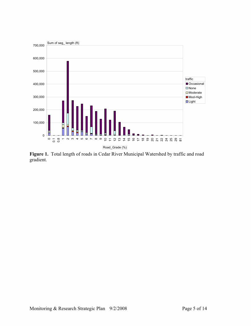
Monitoring & Research Strategic Plan 9/2/2008 Page 5 of 14

0

100,000

200,000

300,000

400,000

500,000

600,000

700,0000

0.1

0.8 1 2 3 4 5 6 7 8 9 10 11 12 13 14 15 16 17 18 19 20 21 22 24 25 29 81

OccasionalNoneModerateMod-HighLight

Sum of seg_ length (ft)

Road_Grade (%)

traffic

Figure 1. Total length of roads in Cedar River Municipal Watershed by traffic and road gradient.

Monitoring & Research Strategic Plan 9/2/2008 Page 6 of 14

0

200,000

400,000

600,000

800,000

1,000,000

1,200,000

1,400,000

Asphalt

Ballast_RockBorrow

Crushed_Rock

Native_Blocky_Coarse

Native_Blocky_Med/Fine

Native_Fines

Native_Blocky

OccasionalNoneModerateMod-HighLight

Sum of seg_ length (ft)

Road Surfac

traffic

Figure 2. Total length of roads in Cedar River Municipal Watershed by traffic and surfacing (Note: based on 2005 inventory; 100/200 roads – light native blocky – are now crushed surfacing)

Monitoring & Research Strategic Plan 9/2/2008 Page 7 of 14

0

50

100

150

200

250

0-100

100-2

00

200-3

00

300-4

00

400-5

00

500-6

00

600-1

000

1000

-2000

2000

-3000

>300

0

Length of each segment (ft)

Freq

uenc

y (#

of s

egm

ents

in e

ach

cate

gory

)

DirectVia gully

Figure 3. Length of direct delivery and direct via gully road segments in Cedar River Municipal Watershed. Critical Question 2: How accurate are the WARSEM predictions of delivery of eroded sediments in the CRMW?

Justification: The WARSEM model uses data from a road research study in Idaho to estimate the distance sediment can be transported from the outlet of a culvert (Ketcheson and Megahan 1996). The Idaho study site conditions were different than those in the CRMW (Idaho – sandy soil, Cedar – finer-grained soil, different precipitation patterns and intensities). Improving our understanding of the distances and associated site characteristics where sediment delivery across the forest floor occurs will greatly improve our confidence in sediment predictions and the implementation of future road improvements designed to reduce sediment delivery to streams. Scope of Study: The proposed study method would be to install filter fabric structures (similar to silt fences) to catch runoff at varying distances below culvert outfalls and at dispersed runoff sites. This study would require 35 sample sites monitored over 3 years (5 sites each – 10, 25, 50, 100, 200 ft from outfall and 10 and 20 ft from dispersed sites). Sites would be visually checked twice/year to determine if road sediment reaches filter structure.

Critical Question 3: What is the actual reduction of road surface erosion due to road work in the CRMW?

Justification: A great deal of effort has and will continue to be expended to reduce sediment input from roads in the watershed. A measure of the success of this effort is

Monitoring & Research Strategic Plan 9/2/2008 Page 8 of 14

important to help determine the cost effectiveness of these actions. Common expensive measures used to address this issue include surfacing (gravel), grading, ditching/cleaning, armoring ditches, addition of culverts, vegetation management, and installation of silt fencing. Scope of Study: Sampling the effectiveness of BMPs requires either a paired segment study (one segment without BMP, another similar one with the BMP) or monitoring of a single segment without the BMP for several years, adding the BMP, and monitoring the segment with the BMP for several years. Recommended BMPs to measure are:

• Adding gravel • Grading • Ditching/cleaning • Armoring ditches

If time is a critical factor (want to know the answer sooner), 8 additional monitoring stations (2 for each BMP) could be added to selected segments adjacent to those in Table 1. If time is not as critical, 8-10 of the segments from Table 1 could be chosen to monitor for 2 years under existing conditions, then BMPS could be added and monitored for 2-3 additional years.

Critical Question 4: How much sediment is produced from low traffic roads in the CRMW

Justification: One important objective of road decommissioning work in the CRMW is the reduction of sediment delivering from nonessential roads. Understanding the amount of road surface erosion produced from these roads will inform our prioritization, enabling us to more confidently identify and prioritize roads where significant sediment delivery to streams and wetlands is occurring. Scope of Study: A measure of sediment production from low use roads is included in Critical Question 1.

Critical Question 5: How much sediment is produced from road use/alterations associated with temporary, project-related effects (e.g., thinning operations)

Justification: Temporary changes in traffic patterns and road maintenance and reconstruction are associated with special projects such as thinning operations in the watershed. Disturbance associated with special projects generally last less than one year and will continue at various locations in the future. These temporary changes likely result in a temporary increase in sediment production from the affected areas. Research in other locations suggests the temporary increases from only changes in traffic use return to normal levels in a short period of time (days to weeks; Reid 1982), but increases from road reconstruction take 2-3 years to return to pre-disturbance levels (Ketcheson et. al 1999, Luce and Black 1999, Grace 1999, Swift 1984, Dryness 1975, Megahan 1974, Megahan and Kidd 1972). Scope of Study: The most cost-effective way to address this question would be to find a location where thinning/road reconstruction efforts are planned for 2010-2011 adjacent to current low traffic roads. Road segments would be monitored for 2 years under low use conditions (Critical Question 1 and 4), continue to be monitored during the thinning/reconstruction efforts, and for 2-3 years following this work (total time 5-6

Monitoring & Research Strategic Plan 9/2/2008 Page 9 of 14

years). This would provide information on low use road erosion rates, changes due to temporary disturbance, length of time to recover, and, if BMPs are planned (Critical Question 3), the effectiveness of these measures (assuming several sites are left with no BMPs). These sites could be included in Critical Question 1 and 3 estimates (segments selected from Table 1).

Critical Question 6: How much sediment is produced and delivered from high use roads adjacent to key water features?

Justification: Traffic use, particularly during wet weather, has been shown to greatly increase sediment production from road surfaces. Several high use roads are located adjacent to waterways in the CRMW with a high likelihood of delivery of the sediment to water bodies. A measure of the amount of sediment produced by these roads would provide information on the importance of controlling sediment from these roads. Scope of Study: A measure of sediment production from high use roads is included in Critical Question 1. Delivery is included in Critical Question 2.

Critical Question 7: Do the road segments WARSEM predicted to be the highest sediment producers actually produce large quantities of sediment?

Justification: The top 20 WARSEM-predicted road segments have the following characteristics: direct/direct via gully delivery, long segment lengths (500-2,500 feet), native surfacing (all but 2), high gradient (7-20%), and varying traffic rates. Scope of Study: Directly sampling the predicted high sediment producers is a great goal. However, the long lengths (most over 800 feet long) would preclude them from being part of the “constant length” pool of study segments discussed in Critical Question 1. It would be worthwhile to visit several of these in the field to determine if it would be feasible (space for sampling equipment?) to monitor 2-3 of these segments. If so, it would add 2-3 additional monitoring stations for 3 years.

5.0 Methods Different researchers have measured road surface erosion using a number of methods through the years. Two separate data collection methodologies are proposed for the current study:

• Road surface erosion sampling using a settling tank (with optional tipping bucket at select plots) based on Black and Luce (2007)

• Sediment delivery distance sampling using silt fence traps set at pre-determined distances downslope of selected road segments (Robichaud and Brown 2002).

Electronic versions of both methodologies are provided separately that include implementation details, materials lists, and sampling techniques. The two techniques are summarized below. Road Surface Erosion Sampling Road surface erosion sampling will measure the amount of sediment produced from road segments. Black and Luce (2007 Draft) have developed a cost-effective method for measuring surface erosion using a bordered road erosion plot, a settling tank, and an optional tipping bucket/flow sampling device. The advantages to this methodology are that it is comparatively

Monitoring & Research Strategic Plan 9/2/2008 Page 10 of 14

low cost, requires only periodic checking (annually if only the settling tank is used; monthly data downloads for the tipping bucket device), and collected data is comparable to other data that is being collected in the Pacific Northwest using the same equipment. Road segments to be measured are isolated from other road segments by the use of constructed wood/rubber waterbars that direct runoff from the measured road segment into the ditchline. A ditch diversion structure directs the runoff into a 6” corrugated plastic pipe that carries water under the road and flows into a steel settling tank on the downslope side of the road (alternatively, an existing culvert can be used to divert water under road). The coarse sediment (and some fraction of the fine-grained silt and clay) settle and remain in the tank. If information on fine-grained sediment is important, water that spills out of the tank can be directed into a tipping bucket flow monitor attached to a datalogger that records runoff volume and takes a sub-sample of runoff to estimate suspended sediment concentration. Estimated cost per sample to install and monitor a road segment for 3 years is $5,200 without the tipping bucket, or $12,100 with the tipping bucket option (note: costs for tipping buckets assume SPU shop fabrication. Costs with pre-made tipping bucket are $10,390.) Delivery Distance In addition to sediment production, road models estimate the percent of eroded sediment that is delivered to a stream or water body based on the distance between the road runoff point (e.g., culvert outfall) and the stream. The WARSEM model assumes that 35% of the sediment produced from a road segment located between 1-100 feet from a stream is delivered to a stream, and 10% of the sediment is delivered from segments located between 101-200 feet from a stream. These estimates are based on research in the Idaho batholith (sandy soils, sparse vegetation) and likely overestimate delivery in the CRMW, with its dense vegetation that helps trap sediment traveling across the forest floor. Installation of silt fence sediment traps on hillsides downslope of road segments is proposed to measure how far road sediment is transported from a road. Silt fence methodologies are described in Robichaud and Brown (2002). In order to measure sediment transport distances, silt fence traps would be installed 10, 25, 50, 100, 200 ft downslope from culvert outfalls, and 10 and 20 ft downslope from dispersed sites (e.g., outsloped road segments). Robichaud and Brown recommend a minimum of 5 replicates per site, resulting in 35 total sites. Silt fence locations would be visited twice/year to determine if any sediment is collecting at them. If so, sediment would be collected and weighed to determine quantity reach the silt fence. Estimated cost for installing and monitoring a silt fence location for 3 years is $1,240. 6.0 Estimated Project Cost An estimate of total project cost was made based on total number of samples to answer all critical questions listed in Table and estimated costs to install and monitor sample locations for three years (Table 2, Scenario 1). Scenario 2 (Table 2) includes all plots listed in Table 1, but only 5 tipping bucket plots (which would be used to extrapolate percent fines overflowing the settling basins in the other 45 erosion samples – would introduce some error by extrapolating).

Monitoring & Research Strategic Plan 9/2/2008 Page 11 of 14

Scenario 3 (Table 2) reduces the number of sample sites on occasional traffic roads from 20 to 12 and includes 5 tipping bucket plots. The 5 sites on WARSEM-estimated highest yield road segments (QC 7) are also dropped in scenario 3 because the reason these road segments have the highest yields is primarily due to the fact that they are very long (would get same amount by adding together several shorter segments). The reasoning behind reducing the number of sample sites on occasional traffic roads is that these likely produce very little sediment (although they account for 80% of the road length in the watershed). Table 2. Estimated Sampling Costs Scenario 1. All sample sites listed in Table 1

Sampling Method Number of plots Cost/plot Total

Road Erosion Plots, no tipping bucket 25 $5,160.45 $113,976.00Road Erosion Plots, with tipping bucket 25 $12,109.28 $302,731.88 Silt fence plots 35 $ 1,243.00 $ 43,505.00 TOTAL 50 + 35 $ 475,248.13

Scenario 2. All sample sites listed in Table 1; only 5 tipping buckets

Sampling Method Number of plots Cost/plot Total

Road Erosion Plots, no tipping bucket 45 $ 5,160.45 $ 232,220.25 Road Erosion Plots, with tipping bucket 5 $12,109.28 $ 60,546.38 Silt fence plots 35 $ 1,243.00 $ 43,505.00 TOTAL 50 + 35 $ 336,271.63

Scenario 3. Fewer occasional traffic road sites (9); does not address QC 7, 5 tipping buckets

Sampling Method Number of plots Cost/plot Total

Road Erosion Plots, no tipping bucket 32 $ 5,160.45 $ 165,134.40 Road Erosion Plots, with tipping bucket 5 $12,109.28 $ 60,546.38 Silt fence plots 35 $ 1,243.00 $ 43,505.00 TOTAL 37 + 35 $ 269,185.78

7.0 Proposed Pilot Project Given the large overall expense and difficulty predicting installation costs, an initial smaller-scale study is proposed to help refine project costs as well as provide a means to gain familiarity with the construction and installation of monitoring equipment. The pilot project would include both the road erosion plot and silt fence monitoring locations and would be aimed at calibrating the WARSEM erosion estimates (QC1, QC2) and estimating the effectiveness of the road erosion reduction strategies most commonly employed in the watershed (surfacing and installing culverts to reduce delivery, QC 4). Table 3 lists proposed pilot project sample site locations in relation to the Critical Questions. Road erosion plot sample site locations were chosen to answer Critical Questions 1, 4, and 6 across most traffic levels. The Moderately High traffic level was dropped since most of these segments are on the Kerriston Road which is not owned by SPU. Note also that Light traffic,

Monitoring & Research Strategic Plan 9/2/2008 Page 12 of 14

Native medium/fine surfacing category from Table 1 and Figure 2 have been revised to crushed surfacing in Table 3 since these segments are primarily along the 100 and 200 road systems which have been re-surfaced since the 2005 road inventory. Table 3. Potential Sample Site Characteristics and Recommended Sample Size for Pilot Project

Traffic Surfacing Gradient Total Notes Critical Questions 1, 4, and 6

Borrow 5-7% 2 Native blocky/coarse 5-7% 2

Native Medium/fine 5-7% 3 (1 w/ tipping bucket) Occasional

Native fine 5-7% or 10-12%

1 w/ tipping bucket

Effects of gradient are well documented in

literature, so concentrate most samples in 5-7%

gradient range if possible

Borrow 5-7% 3

Light Crushed 2-3% 3 (1 w/ Tipping bucket)

Would like to install one station each on the 100

and 200 road since these deliver directly to lake

Borrow 2-3% Moderate Crushed 2-3% 2

Moderately High Crushed 2-3%, 7% 0

Majority of this category is Kerriston Road – not

owned by SPU Additional silt fence monitoring sites at the 8 occasional use road sites 8 Install on road segments

adjacent to erosion plots Critical Question 3 Either select segments from Critical Question (CQ)1 and monitor for an additional 2-3 years, or add paired BMP segments to initial study

None

Critical Question 5

Select low use segments from CQ1 in areas that will have special projects in 2010-2011 None

If possible, select Occasional use roads

from QC 1 that will have higher traffic levels in

year 2 or 3 of pilot study Critical Question 7 Select 5 of highest predicted segments to monitor; these are longer lengths – would test difference in length of segment (is adding culverts to break up lengths helpful?)

None

Critical Question 2 Silt fence monitoring sites 15 Total Segments: Road Erosion Plots - 16 (3 w/tipping buckets); Silt fence plots - 15 Since the effects of gradient on erosion are fairly well documented in the literature (Dubé et al. 2004), and a check of 2-3% gradient occasional use roads in the field showed that many of these roads are on grade (not enough side slope to place settling tanks), concentrating on the 5-7%

Monitoring & Research Strategic Plan 9/2/2008 Page 13 of 14

gradient road segments for sample locations is recommended. The exception is the 100 and 200 road systems (light traffic use category). These roads are low gradient (1-3%) but many segments are located adjacent to the reservoir with adequate sideslope gradient and space to install settling basins. The 15 silt fence monitoring sites chosen to address Critical Question 2 will also provide information on the effectiveness of adding culverts to break up road segments and reduce delivery by directing road runoff to the forest floor. Occasional use roads account for the majority of roads in the CRMW (Figure 2). However, based on the WARSEM model, erosion measurements on roads in other areas, and observations of the lack of sediment in ditchlines along occasional use roads in the CRMW, it is likely that these roads produce little sediment. Half of the sediment monitoring plots with settling tanks are proposed to be installed on occasional use roads. Since installation and monitoring of the settling tanks is somewhat expensive, it is proposed that silt fence sediment traps be installed at culvert outfalls at road segments adjacent to the settling tank plots. Assuming that all else (slope, geology, traffic, surfacing) would be equal between adjacent segments, this will allow us to compare methods and test whether or not the most cost-effective silt fences could be employed to collect data along occasional use roads. The estimated 2008 installation costs for the pilot project are listed in Table 4 along with total costs for 3 years of data collection. Table 4. Estimated Costs for Proposed Pilot Project

Sampling Method Number of

plots

Cost/plot (installation

only) Cost in

2008

Total Costs (3-year data

collection and analysis)

Road Erosion Plots, no tipping bucket 13 $2,910.75 $37,840 $50,798 Road Erosion Plots, w/pre-made tipping bucket 3 $4,063.75 $12,191 $22,310

Silt fences at erosion stations 8 $494.50 $3,956 $7,148 Silt fences for delivery distance 15 $494.50 $7,418 $13,403

TOTAL 16 erosion, 23 silt fence

$61,405 $93,658

Note: placing traffic counters (SPU already owns several) along several of the higher use road segments selected for monitoring would provide site-specific information on traffic levels. It is possible that some traffic counters will be deployed in the watershed for other purposes and may be on roads being monitored for sediment. 8.0 References Black, T.A. and C.H. Luce 2007. Measuring water and sediment discharge from a bordered road

plot using a settling basin and tipping bucket. Unpublished paper dated 8.15.07

Monitoring & Research Strategic Plan 9/2/2008 Page 14 of 14

Dryness, C.T., 1975. Grass-legume mixtures for erosion control along forest roads in Western Oregon. Journal of Soil and Water Conservation, July-Aug. 1975, pp. 169-173.

Dubé, K., W. Megahan, and M. McCalmon, 2004. Washington road surface erosion model. Unpublished report prepared for the State of Washington Department of Natural Resources. February 20, 2004. Available to download at: http://www.dnr.wa.gov/forestpractices/adaptivemanagement/cmer/warsem/

Grace, J.M., III. 1999. Erosion control techniques on forest road cutslopes and fillslopes in North Alabama. In: Seventh International Conference on Low Volume Roads. Volume 2; Transportation Research Record 1652; pp. 227-234.

Ketcheson, G.L. and W.F. Megahan, 1996. Sediment production and downslope sediment transport from forest roads in granitic watersheds. USDA Forest Service, Intermountain Research Station. Research Paper INT-RP0486.

Ketcheson, G.L., W.F. Megahan, and J.G. King, 1999. “R1-R4” and “BOISED” sediment prediction model tests using forest roads in granitics. Journal of the American Water Resources Association Vol. 35, No. 1, pp. 83-98.

Luce, C.H. and T.A. Black, 1999. Spatial and temporal patterns in erosion from forest roads. In: M.S. Wigmosta and S.J. Burgess, eds. The Influence of Land Use on the Hydrologic-Geomorphic Responses of Watersheds. AGU Monographs.

Megahan, W.F., 1974, Erosion over time on severely disturbed granitic soils: a model: USDA Forest Service Intermountain Research Station General Technical Report INT-156, Boise, ID.

Megahan, W.F., and G.L. Ketcheson, 1996. Predicting downslope travel of granitic sediments from forest roads in Idaho. Water Resources Bulletin, Vol. 32, No. 2, pp. 371-382.

Megahan, W.F. and W.J. Kidd. 1972. Effects of logging and logging roads on erosion and sediment deposition for steep terrain. Journal of Forestry.

Reid, L.M, 1981. Sediment production from gravel-surfaced forest roads, Clearwater Basin, Washington. M.S. Thesis, University of Washington.

Robichaud, P.R. and R.E. Brown, 2002. Silt fences: an economical technique for measuring hillslope soil erosion. USDA Forest Service general technical report RMRS-GTR-94. August 2002.

Swift, L.W. Jr., 1984. Gravel and grass surfacing reduces soil loss from mountain roads. Forestry Science, Vol. 30, pp.657-670.