Critical exponents of the 3-D Ising model

arX

iv:c

ond-

mat

/960

1048

v1 1

5 Ja

n 19

96

LA UR-96-93

CRITICAL EXPONENTS OF THE 3-D ISING MODEL

Rajan Gupta* §

T-8, MS-B285, Los Alamos National Laboratory, Los Alamos, NM 87545

Pablo Tamayo †

T-8, MS-B285, Los Alamos National Laboratory, Los Alamos, NM 87545

and

Thinking Machines Corporation, Cambridge, MA 02143, USA

ABSTRACT

We present a status report on the ongoing analysis of the 3D Ising model with nearest-neighbor interac-tions using the Monte Carlo Renormalization Group (MCRG) and finite size scaling (FSS) methods on 643,1283, and 2563 simple cubic lattices. Our MCRG estimates are Kc

nn = 0.221655(1)(1) and ν = 0.625(1).The FSS results for Kc are consistent with those from MCRG but the value of ν is not. Our best estimateη = 0.025(6) covers the spread in the MCRG and FSS values. A surprise of our calculation is the estimateω ≈ 0.7 for the correction-to-scaling exponent. We also present results for the renormalized coupling gR

along the MCRG flow and argue that the data support the validity of hyperscaling for the 3D Ising model.

Date = 1/14/96

* Invited talk presented at the US-Japan Bilateral Seminar, Maui, August 28-31, 1995. To be published in

International Journal of Modern Physics C.

§ [email protected]

† [email protected].

1. Introduction

The 3D Ising model has, over the last 25 years, been used to test the accuracy of various analytical andnumerical methods for solving Statistical Mechanics systems. In 1992 we presented results of simulationson 643 and 1283 lattices using the Monte Carlo Renormalization Group (MCRG) method [1]. While thatwork improved on previous MCRG estimates [2] [3]), it left us with four unanswered questions. The firstand most tantalizing was −− are the exponents rational numbers, i.e. ν = 0.625 and η = 0.025. Second,a more precise determination of the corrections-to-scaling exponent is needed as it is the largest source ofsystematic errors. Third, we wanted to resolve/understand the differences between our MCRG and existingfinite size scaling/ ǫ-expansion results. Lastly, we wanted to investigate whether hyperscaling holds for thismodel. This talk is a summary of the current status of our calculations.

In order to address these issues we have extended the calculations in the following ways. We have madehigher statistics runs on 643, 1283, and 2563 lattices at K = 0.221652 and 0.221655. On these latticeswe have evaluated, in addition to correlation functions needed for MCRG studies, quantities needed forfinite size scaling (FSS) analysis and the calculation of the renormalized coupling gR. As a result we havebetter estimates of the critical coupling Kc

nn, the exponents ν and η from both MCRG and finite-size scaling(including histogram re-weighting) analysis, and can address the issue of hyperscaling violations. Our newestimate of the corrections-to-scaling exponent ω ≈ 0.7 is significantly smaller than that from other methods.

All the simulations have been done on the Thinking Machines CM-5 (at the ACL at LANL) and CM-5E(at TMC) computers. We used the Swendsen-Wang cluster update algorithm [4] and a 250-long 64-bit wideshift-register (Kirkpatrick-Stoll) random number generator in each vector unit. The new results agree withour previous calculation and those in [2] and [3]. Each of these calculations used a different random numbergenerator, so their consistency suggests that there is no obvious bias in the sequence of random numbersgenerated (see P. Coddington’s talk on random number generators at this workshop). Our most extensiveresults are at Knn = 0.221655, which is our present best estimate of Kc, and the statistical sample consistsof 600K, 500K, and 400K measurements on 643, 1283, and 2563 lattices respectively.

The details of our implementation of the MCRG method are the same as in [1]. The only change isthat we have added 3 more even couplings (for a total of 56) and one more odd couplings (total 47). Theoriginal 53 even and 46 odd couplings were contained in either a 3× 3 square or a 23 template [1]. The newcouplings are those obtained by adding a fourth spin along the cartesian axis to the 3 × 3 template.

We store the magnetization and energy for each configuration, from which we can calculate quantitieslike the specific heat, susceptibility, Binder’s cumulant U = 3 − 〈m4〉/〈m2〉2, etc.. These results are thenevaluated as a function of K, in a small neighborhood of Ksimulation, using the histogram re-weightingmethod [5]. The finite size analysis of these quantities follows the work of Ferrenberg and Landau [6], i.e.without corrections to scaling terms. To calculate gR, we also need the finite lattice correlation length ξ.This is calculated in two ways:

〈∑

x,y

s(x, y, z)∑

x,y

s(x, y, 0)〉−→

z→∞ ae−z/ξ,

1

k2

(

S(0)2

S(k)2− 1

)

= ξ2 ,

(1.1)

where S(k) =∑

x,y,z s(x, y, z)ei~k·~x. We investigate the 5 lowest momenta but present results only for thelowest, kz = 2π/L, as it has the best signal. With ξ in hand we calculate gR defined as [7]

gR(K, L) =(L

ξ

)d(

3 −〈m4〉

〈m2〉2

)

. (1.2)

This is expected to scale asgR(K, L) ∼ L−w∗

(1.3)

where w∗ = (γ + dν − 2∆)/ν is referred to as the anomalous dimension of the vacuum. If hyperscaling holdsthen g∗R → finite non-zero constant as L → ∞ and K → K∗.

For the purpose of error analysis the data have been divided into bins of size 10,000 measurements. Allerrors are then calculated by a single elimination jackknife procedure over these bins. This talk is organizedas follows. We first summarize the MCRG results, then compare them with FSS estimates, and finally givedata for gR, both at Ksim = 0.221655 and along the MCRG flow, and discuss hyperscaling.

1

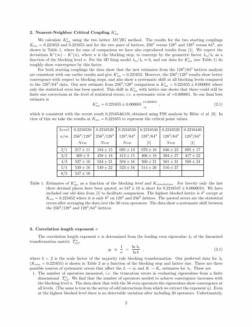
2. Nearest-Neighbor Critical Coupling Kcnn

We calculate Kcnn using the two lattice MCRG method. The results for the two starting couplings

Knn = 0.221652 and 0.221655 and for the two pairs of lattices, 2563 versus 1283 and 1283 versus 643, areshown in Table 1, where for ease of comparison we have also reproduced results from [1]. We expect thedeviations Kc(∞) − Kc(n), where n is the blocking step, to converge by the geometric factor λu/λt as afunction of the blocking level n. For the 3D Ising model λu/λt ≈ 6, and our data for Kc

nn (see Table 1) doroughly show convergence by this factor.

For both starting couplings the data show that the new estimates from the 1283/643 lattices analysisare consistent with our earlier results and give Kc

nn = 0.221652. However, the 2563/1283 results show betterconvergence with respect to blocking steps, and also show a systematic shift at all blocking levels comparedto the 1283/643 data. Our new estimate from 2563/1283 comparison is Kc

nn = 0.221655 ± 0.000001 whereonly the statistical error has been quoted. This shift in Kc

nn with lattice size shows that there could still befinite size corrections at the level of statistical errors, i.e. a systematic error of +0.000001. So our final bestestimate is

Kcnn = 0.221655± 0.000001

+0.000001

−0, (2.1)

which is consistent with the recent result 0.2216546(10) obtained using FSS analysis by Blote et al. [8]. Inview of this we take the results at Knn = 0.221655 to represent the critical point values.

Level 0.2216550 0.2216520 0.2216550 0.2216540 0.2216520 0.2216440

n/m 2563/1283 2563/1283 1283/643 1283/643 1283/643 1283/643

New New New [1] New [1]

2/1 217 ± 11 184 ± 15 095 ± 13 070 ± 16 046 ± 23 095 ± 17

3/2 469 ± 9 458 ± 18 413 ± 15 406 ± 18 394 ± 27 417 ± 22

4/3 537 ± 10 534 ± 21 504 ± 16 500 ± 21 501 ± 31 508 ± 24

5/4 549 ± 10 549 ± 22 523 ± 16 514 ± 26 516 ± 37

6/5 547 ± 10

Table 1. Estimates of Kcnn as a function of the blocking level and Ksimulation. For brevity only the last

three decimal places have been quoted, so 547 ± 10 is short for 0.2216547 ± 0.0000010. We haveincluded our old data from [1] to facilitate comparison. The highest blocked lattice is 43 except atKnn = 0.221652 where it is only 83 on 1283 and 2563 lattices. The quoted errors are the statisticalerrors after averaging the data over the 56 even operators. The data show a systematic shift betweenthe 2563/1283 and 1283/643 lattices.

3. Correlation length exponent ν

The correlation length exponent ν is determined from the leading even eigenvalue λt of the linearizedtransformation matrix T n

αβ ,

yt ≡1

ν=

lnλt

ln b, (3.1)

where b = 2 is the scale factor of the majority rule blocking transformation. Our preferred data for λt

(Ksim = 0.221655) is shown in Table 2 as a function of the blocking step and lattice size. There are threepossible sources of systematic errors that affect the L → ∞ and K → Kc estimates for λt. These are

1. The number of operators measured, i.e. the truncation errors in evaluating eigenvalues from a finitedimensional T n

αβ . We find that the number of operators needed to achieve convergence increases withthe blocking level n. The data show that with the 56 even operators the eigenvalues show convergence atall levels. (The same is true in the sector of odd interactions from which we extract the exponent η). Evenat the highest blocked level there is no detectable variation after including 30 operators. Unfortunately,

2

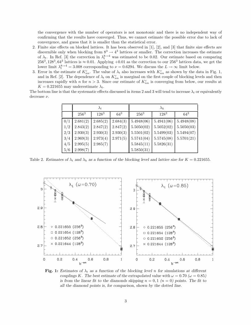
the convergence with the number of operators is not monotonic and there is no independent way ofconfirming that the results have converged. Thus, we cannot estimate the possible error due to lack ofconvergence, and guess that it is smaller than the statistical error.

2. Finite size effects on blocked lattices. It has been observed in [1], [2], and [3] that finite size effects arediscernible only when blocking from 83 → 43 lattices or smaller. The correction increases the estimateof λt. In Ref. [3] the correction in λ8→4

t was estimated to be 0.02. Our estimate based on comparing2563, 1283, 643 lattices is ≈ 0.01. Applying +0.01 as the correction to our 2563 lattices data, we get thelower limit λ8→4

t = 3.008 corresponding to ν = 0.6294. We discuss the L → ∞ limit below.3. Error in the estimate of Kc

nn. The value of λt also increases with Kcnn as shown by the data in Fig. 1,

and in Ref. [2]. The dependence of λt on Kcnn is marginal on the first couple of blocking levels and then

increases rapidly with n for n > 3. Since our estimate of Kcnn is converging from below, our results at

K = 0.221655 may underestimate λt.The bottom line is that the systematic effects discussed in items 2 and 3 will tend to increase λt or equivalentlydecrease ν.

λt λh

2563 1283 643 2563 1283 643

0/1 2.681(2) 2.685(2) 2.684(3) 5.4948(06) 5.4941(06) 5.4948(08)

1/2 2.843(2) 2.847(2) 2.847(2) 5.5050(02) 5.5052(02) 5.5050(03)

2/3 2.930(3) 2.930(3) 2.930(3) 5.5501(02) 5.5499(03) 5.5494(07)

3/4 2.969(3) 2.973(4) 2.971(5) 5.5741(04) 5.5745(08) 5.5701(21)

4/5 2.995(5) 2.985(7) 5.5845(11) 5.5826(31)

5/6 2.998(7) 5.5850(31)

Table 2. Estimates of λt and λh as a function of the blocking level and lattice size for K = 0.221655.

Fig. 1: Estimates of λt as a function of the blocking level n for simulations at differentcouplings K. The best estimate of the extrapolated value with ω = 0.70 (ω = 0.85)is from the linear fit to the diamonds skipping n = 0, 1 (n = 0) points. The fit toall the diamond points is, for comparison, shown by the dotted line.

3

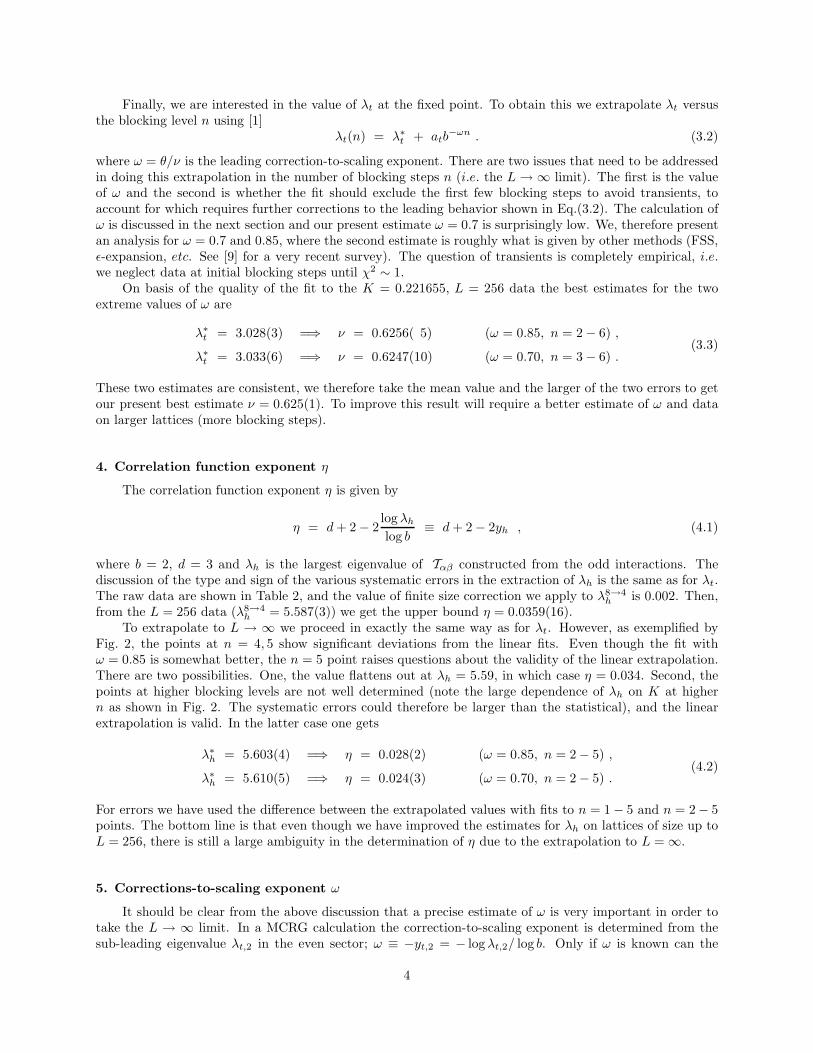
Finally, we are interested in the value of λt at the fixed point. To obtain this we extrapolate λt versusthe blocking level n using [1]

λt(n) = λ∗t + atb

−ωn . (3.2)

where ω = θ/ν is the leading correction-to-scaling exponent. There are two issues that need to be addressedin doing this extrapolation in the number of blocking steps n (i.e. the L → ∞ limit). The first is the valueof ω and the second is whether the fit should exclude the first few blocking steps to avoid transients, toaccount for which requires further corrections to the leading behavior shown in Eq.(3.2). The calculation ofω is discussed in the next section and our present estimate ω = 0.7 is surprisingly low. We, therefore presentan analysis for ω = 0.7 and 0.85, where the second estimate is roughly what is given by other methods (FSS,ǫ-expansion, etc. See [9] for a very recent survey). The question of transients is completely empirical, i.e.we neglect data at initial blocking steps until χ2 ∼ 1.

On basis of the quality of the fit to the K = 0.221655, L = 256 data the best estimates for the twoextreme values of ω are

λ∗t = 3.028(3) =⇒ ν = 0.6256( 5) (ω = 0.85, n = 2 − 6) ,

λ∗t = 3.033(6) =⇒ ν = 0.6247(10) (ω = 0.70, n = 3 − 6) .

(3.3)

These two estimates are consistent, we therefore take the mean value and the larger of the two errors to getour present best estimate ν = 0.625(1). To improve this result will require a better estimate of ω and dataon larger lattices (more blocking steps).

4. Correlation function exponent η

The correlation function exponent η is given by

η = d + 2 − 2log λh

log b≡ d + 2 − 2yh , (4.1)

where b = 2, d = 3 and λh is the largest eigenvalue of Tαβ constructed from the odd interactions. Thediscussion of the type and sign of the various systematic errors in the extraction of λh is the same as for λt.The raw data are shown in Table 2, and the value of finite size correction we apply to λ8→4

h is 0.002. Then,from the L = 256 data (λ8→4

h = 5.587(3)) we get the upper bound η = 0.0359(16).To extrapolate to L → ∞ we proceed in exactly the same way as for λt. However, as exemplified by

Fig. 2, the points at n = 4, 5 show significant deviations from the linear fits. Even though the fit withω = 0.85 is somewhat better, the n = 5 point raises questions about the validity of the linear extrapolation.There are two possibilities. One, the value flattens out at λh = 5.59, in which case η = 0.034. Second, thepoints at higher blocking levels are not well determined (note the large dependence of λh on K at highern as shown in Fig. 2. The systematic errors could therefore be larger than the statistical), and the linearextrapolation is valid. In the latter case one gets

λ∗h = 5.603(4) =⇒ η = 0.028(2) (ω = 0.85, n = 2 − 5) ,

λ∗h = 5.610(5) =⇒ η = 0.024(3) (ω = 0.70, n = 2 − 5) .

(4.2)

For errors we have used the difference between the extrapolated values with fits to n = 1 − 5 and n = 2 − 5points. The bottom line is that even though we have improved the estimates for λh on lattices of size up toL = 256, there is still a large ambiguity in the determination of η due to the extrapolation to L = ∞.

5. Corrections-to-scaling exponent ω

It should be clear from the above discussion that a precise estimate of ω is very important in order totake the L → ∞ limit. In a MCRG calculation the correction-to-scaling exponent is determined from thesub-leading eigenvalue λt,2 in the even sector; ω ≡ −yt,2 = − logλt,2/ log b. Only if ω is known can the

4

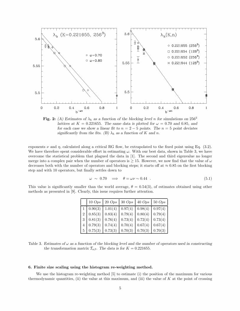
Fig. 2: (A) Estimates of λh as a function of the blocking level n for simulations on 2563

lattices at K = 0.221655. The same data is plotted for ω = 0.70 and 0.85, andfor each case we show a linear fit to n = 2 − 5 points. The n = 5 point deviatessignificantly from the fits. (B) λh as a function of K and n.

exponents ν and η, calculated along a critical RG flow, be extrapolated to the fixed point using Eq. (3.2).We have therefore spent considerable effort in estimating ω. With our best data, shown in Table 3, we haveovercome the statistical problem that plagued the data in [1]. The second and third eigenvalue no longermerge into a complex pair when the number of operators is ≥ 15. However, we now find that the value of ωdecreases both with the number of operators and blocking steps; it starts off at ≈ 0.85 on the first blockingstep and with 10 operators, but finally settles down to

ω ∼ 0.70 =⇒ θ = ων ∼ 0.44 . (5.1)

This value is significantly smaller than the world average, θ = 0.54(3), of estimates obtained using othermethods as presented in [9]. Clearly, this issue requires further attention.

10 Ops 20 Ops 30 Ops 40 Ops 50 Ops

1 0.90(3) 1.01(4) 0.97(4) 0.98(4) 0.97(4)

2 0.85(3) 0.83(4) 0.79(4) 0.80(4) 0.79(4)

3 0.81(3) 0.76(4) 0.73(4) 0.72(4) 0.73(4)

4 0.79(3) 0.74(4) 0.70(4) 0.67(4) 0.67(4)

5 0.75(3) 0.73(3) 0.70(3) 0.70(3) 0.70(3)

Table 3. Estimates of ω as a function of the blocking level and the number of operators used in constructingthe transformation matrix Tαβ . The data is for K = 0.221655.

6. Finite size scaling using the histogram re-weighting method.

We use the histogram re-weighting method [5] to estimate (i) the position of the maximum for variousthermodynamic quantities, (ii) the value at this maximum, and (iii) the value of K at the point of crossing

5

of U and gR for two different size lattices. The method consists of building a histogram H(E, m), i.e.the number of configurations with energy E and magnetization m, using an equilibrium (canonical) MonteCarlo simulation at temperature Ksim. With this histogram, the equilibrium probability distribution atother temperatures K is

PK(E, m) =H(E, m) exp[∆KE]

∑

E,m H(E, m) exp[∆KE], (6.1)

where ∆K = K − Ksim. The average value of any function of E and m, Q(E, m), at coupling K is thengiven by

〈QK(E, m)〉 =∑

E,m

Q(E, m)PK(E, m). (6.2)

The value of thermodynamic derivatives with respect to K are obtained from Monte Carlo measurements ofcorrelation functions,

d〈Q〉

dK= 〈QE〉 − 〈Q〉〈E〉. (6.3)

Again, by using the re-weighting technique these correlation functions can be evaluated at all temperatures ina certain neighborhood of Ksim. Thus, the location and magnitude of the peaks, and the points of crossingscan be obtained from simulations at a single temperature.

The propagation of errors under this re-weighting is not straightforward and has been dealt with byFerrenberg and by Swendsen in their talks at this meeting. In our current analysis the error estimates are thenaive statistical ones and ignore all correlations and uncertainty in determining H(E, m). We only presentresults for Ksim = 0.221655 as these have higher statistics and correspond to our estimate of the infinitevolume Kc. With this and the re-weighted data generated from it in hand we use the appropriate finite sizescaling relations to derive estimates of the critical exponents and temperature.

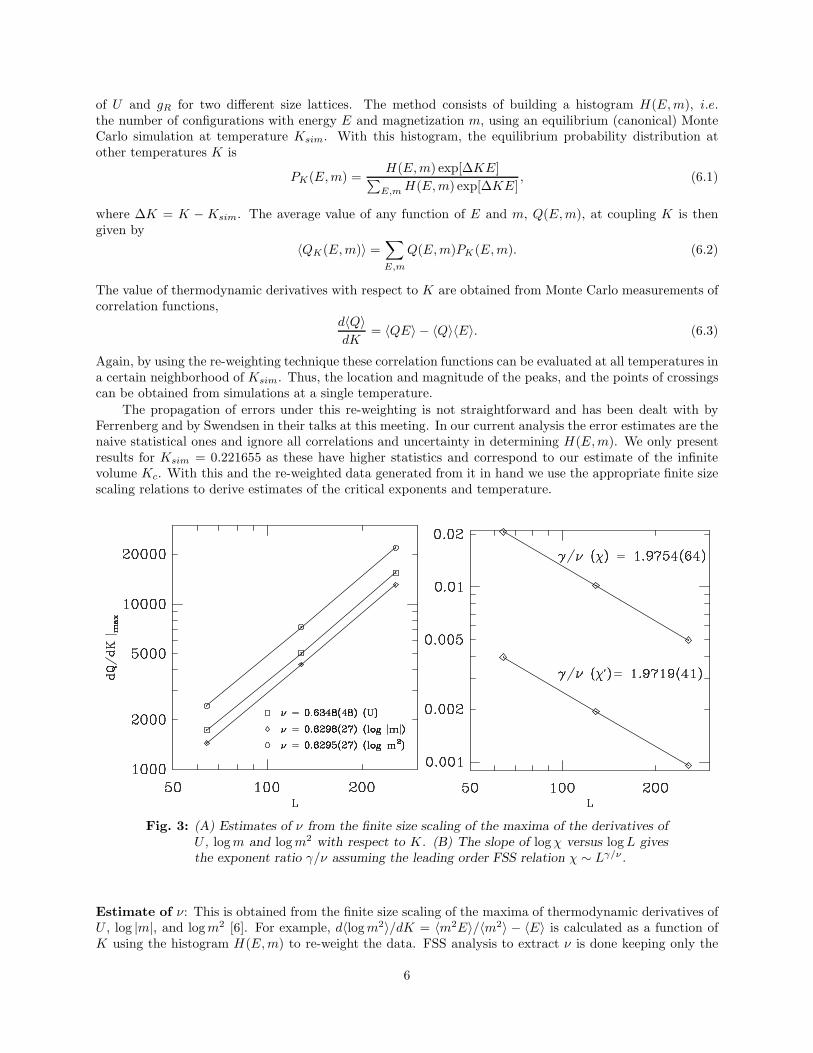
Fig. 3: (A) Estimates of ν from the finite size scaling of the maxima of the derivatives ofU , log m and log m2 with respect to K. (B) The slope of log χ versus log L givesthe exponent ratio γ/ν assuming the leading order FSS relation χ ∼ Lγ/ν .

Estimate of ν: This is obtained from the finite size scaling of the maxima of thermodynamic derivatives ofU , log |m|, and log m2 [6]. For example, d〈log m2〉/dK = 〈m2E〉/〈m2〉 − 〈E〉 is calculated as a function ofK using the histogram H(E, m) to re-weight the data. FSS analysis to extract ν is done keeping only the

6

leading term in the scaling behavior

dQ

dK

∣

∣

∣

∣

max

= aL1/ν(

1 + bL−ω + . . .)

, , (6.4)

as we cannot reliably include correction terms with data at only 3 values of L. Linear fits to the maximumvalue versus L1/ν are shown in Fig. 3. The quality of the fits is exceedingly good, and the final results are

ν = 0.6348(48) U

ν = 0.6298(27) log |m|

ν = 0.6295(27) log m2 .

(6.5)

The values obtained from the derivative of log |m| and log m2 agree, while that from U is higher by its 1σerror estimate. These estimates are higher than the MCRG value by roughly one combined σ.

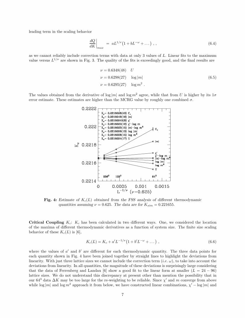
Fig. 4: Estimate of Kc(L) obtained from the FSS analysis of different thermodynamicquantities assuming ν = 0.625. The data are for Ksim = 0.221655.

Critical Coupling Kc: Kc has been calculated in two different ways. One, we considered the locationof the maxima of different thermodynamic derivatives as a function of system size. The finite size scalingbehavior of these Kc(L) is [6],

Kc(L) = Kc + a′L−1/ν(

1 + b′L−ω + . . .)

, (6.6)

where the values of a′ and b′ are different for each thermodynamic quantity. The three data points foreach quantity shown in Fig. 4 have been joined together by straight lines to highlight the deviations fromlinearity. With just three lattice sizes we cannot include the correction term (i.e. ω), to take into account thedeviations from linearity. In all quantities, the magnitude of these deviations is surprisingly large consideringthat the data of Ferrenberg and Landau [6] show a good fit to the linear form at smaller (L = 24 − 96)lattice sizes. We do not understand this discrepancy at present other than mention the possibility that inour 643 data ∆K may be too large for the re-weighting to be reliable. Since χ′ and m converge from abovewhile log |m| and log m2 approach it from below, we have constructed linear combinations, χ′ − log |m| and

7

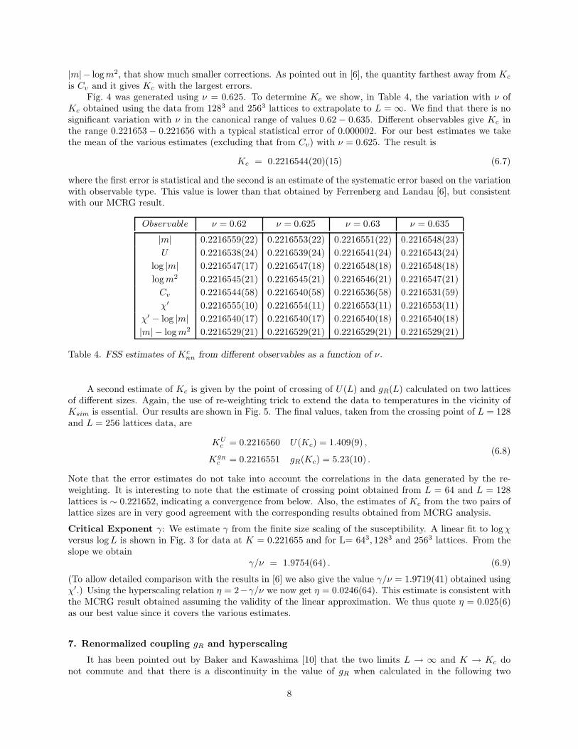
|m| − logm2, that show much smaller corrections. As pointed out in [6], the quantity farthest away from Kc

is Cv and it gives Kc with the largest errors.Fig. 4 was generated using ν = 0.625. To determine Kc we show, in Table 4, the variation with ν of

Kc obtained using the data from 1283 and 2563 lattices to extrapolate to L = ∞. We find that there is nosignificant variation with ν in the canonical range of values 0.62 − 0.635. Different observables give Kc inthe range 0.221653 − 0.221656 with a typical statistical error of 0.000002. For our best estimates we takethe mean of the various estimates (excluding that from Cv) with ν = 0.625. The result is

Kc = 0.2216544(20)(15) (6.7)

where the first error is statistical and the second is an estimate of the systematic error based on the variationwith observable type. This value is lower than that obtained by Ferrenberg and Landau [6], but consistentwith our MCRG result.

Observable ν = 0.62 ν = 0.625 ν = 0.63 ν = 0.635

|m| 0.2216559(22) 0.2216553(22) 0.2216551(22) 0.2216548(23)

U 0.2216538(24) 0.2216539(24) 0.2216541(24) 0.2216543(24)

log |m| 0.2216547(17) 0.2216547(18) 0.2216548(18) 0.2216548(18)

log m2 0.2216545(21) 0.2216545(21) 0.2216546(21) 0.2216547(21)

Cv 0.2216544(58) 0.2216540(58) 0.2216536(58) 0.2216531(59)

χ′ 0.2216555(10) 0.2216554(11) 0.2216553(11) 0.2216553(11)

χ′ − log |m| 0.2216540(17) 0.2216540(17) 0.2216540(18) 0.2216540(18)

|m| − log m2 0.2216529(21) 0.2216529(21) 0.2216529(21) 0.2216529(21)

Table 4. FSS estimates of Kcnn from different observables as a function of ν.

A second estimate of Kc is given by the point of crossing of U(L) and gR(L) calculated on two latticesof different sizes. Again, the use of re-weighting trick to extend the data to temperatures in the vicinity ofKsim is essential. Our results are shown in Fig. 5. The final values, taken from the crossing point of L = 128and L = 256 lattices data, are

KUc = 0.2216560 U(Kc) = 1.409(9) ,

KgR

c = 0.2216551 gR(Kc) = 5.23(10) .(6.8)

Note that the error estimates do not take into account the correlations in the data generated by the re-weighting. It is interesting to note that the estimate of crossing point obtained from L = 64 and L = 128lattices is ∼ 0.221652, indicating a convergence from below. Also, the estimates of Kc from the two pairs oflattice sizes are in very good agreement with the corresponding results obtained from MCRG analysis.

Critical Exponent γ: We estimate γ from the finite size scaling of the susceptibility. A linear fit to log χversus log L is shown in Fig. 3 for data at K = 0.221655 and for L= 643, 1283 and 2563 lattices. From theslope we obtain

γ/ν = 1.9754(64) . (6.9)

(To allow detailed comparison with the results in [6] we also give the value γ/ν = 1.9719(41) obtained usingχ′.) Using the hyperscaling relation η = 2−γ/ν we now get η = 0.0246(64). This estimate is consistent withthe MCRG result obtained assuming the validity of the linear approximation. We thus quote η = 0.025(6)as our best value since it covers the various estimates.

7. Renormalized coupling gR and hyperscaling

It has been pointed out by Baker and Kawashima [10] that the two limits L → ∞ and K → Kc donot commute and that there is a discontinuity in the value of gR when calculated in the following two

8

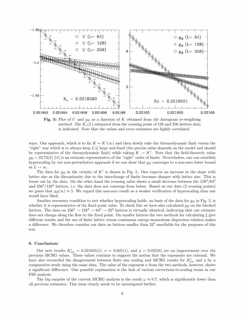
Fig. 5: Plot of U and gR as a function of K obtained from the histogram re-weightingmethod. The Kc(L) estimated from the crossing point of 128 and 256 lattices datais indicated. Note that the values and error estimates are highly correlated.

ways. Our approach, which is to fix K = Kc(∞) and then slowly take the thermodynamic limit versus the“right” way which is to always keep L/ξ large and fixed (the precise value depends on the model and shouldbe representative of the thermodynamic limit) while taking K → Kc. Note that the field-theoretic valuegR = 23.73(2) [11] is an estimate representative of the “right” order of limits. Nevertheless, one can establishhyperscaling by our non-perturbative approach if we can show that gR converges to a non-zero lower boundas L → ∞.

The data for gR in the vicinity of Kc is shown in Fig. 5. One expects an increase in the slope withlattice size as the discontinuity due to the interchange of limits becomes sharper with lattice size. This isborne out by the data. On the other hand the crossing value shows a small decrease between the 1283/643

and 2563/1283 lattices, i.e. the data does not converge from below. Based on our data (2 crossing points)we guess that gR(∞) ≈ 5. We regard this non-zero result as a weaker verification of hyperscaling than onewould have liked.

Another necessary condition to test whether hyperscaling holds, on basis of the data for gR in Fig. 5, iswhether it is representative of the fixed point value. To check this we have also calculated gR on the blockedlattices. The data on 2563 → 1283 → 643 → 323 lattices is virtually identical, indicating that our estimatedoes not change along the flow to the fixed point. On smaller lattices the two methods for calculating ξ givedifferent results and the use of finite lattice versus continuum energy-momentum dispersion relation makesa difference. We therefore consider our data on lattices smaller than 323 unreliable for the purposes of thistest.

8. Conclusions

Our new results Kcnn = 0.221655(1), ν = 0.625(1), and η = 0.025(6) are an improvement over the

previous MCRG values. These values continue to support the notion that the exponents are rational. Wehave also reconciled the disagreement between finite size scaling and MCRG results for Kc

nn and η by acomparative study using the same data. The value of the exponent ν from the two methods, however, showsa significant difference. One possible explanation is the lack of various corrections-to-scaling terms in ourFSS analysis.

The big surprise of the current MCRG analysis is the result ω ≈ 0.7, which is significantly lower thanall previous estimates. This issue clearly needs to be investigated further.

9

The convergence of g∗R, defined to be the crossing point value in the limit L → ∞, seems to be fromabove. Thus, our data does not provide the desired lower bound to validate hyperscaling. We estimateg∗R(L = ∞) from data at the two crossing points to be ∼ 5. If this non-zero value withstands furtherscrutiny, then we will have established that hyperscaling holds for the 3D Ising model.

Acknowledgements

It is a pleasure to thank David Landau and Masuo Suzuki for organizing a very informative workshopin such idyllic surroundings. We thank George Baker and Robert Swendsen for informative discussions. Weare also grateful to the tremendous support provided by the Advanced Computing Laboratory and ThinkingMachines Corporation for this project.

References

[1] C. Baillie, R. Gupta, K. Hawick, and S. Pawley, Phys. Rev. B45 (1992) 10438[2] G. S. Pawley, R. H. Swendsen, D. J. Wallace and K. G. Wilson, Phys. Rev. B29 (1984) 4030.[3] H. W. J. Blote, A. Compagner, J. H. Croockewit, Y. T. J. C. Fonk, J. R. Heringa, A. Hoogland, T. S.

Smit and A. L. van Willigen, Physica A161 (1989) 1.[4] R. Swendsen and J. S. Wang, Phys. Rev. Lett. 58 (1987) 86.[5] A. M. Ferrenberg and R. H. Swendsen, Phys. Rev. Lett. 61 (1988) 2635.[6] A. Ferrenberg, and D. Landau, Phys. Rev. B44 (1991) 5081.[7] B. Freedman and G. Baker, J. Phys. A: Math. Gen. 15 (1982) L715.[8] H. Blote, E. Luijten, and J. Heringa, cond-mat/9509016.[9] S. Zinn and M. Fisher, Maryland Preprint, Nov 1995.

[10] G. Baker and N. Kawashima, Phys. Rev. Lett. 75 (1995) 994.[11] G. Baker, Quantitative Theory of Critical Phenomena, Academic Press, 1990.

10