Crises and Recoveries in an Empirical Model of Consumption Disasters

Crises and Recoveries in an Empirical Model of

Consumption Disasters

Robert Barro

Harvard University

Emi Nakamura

Columbia University

Jon Steinsson

Columbia University

Jose Ursua∗

Harvard University

July 5, 2009

Abstract

We estimate an empirical model of consumption disasters using a new panel data set on

consumption for 24 countries and more than 100 years. The model allows for permanent and

transitory effects of disasters that unfold over multiple years. It also allows the timing of

disasters to be correlated across countries. We estimate the model using Bayesian methods.

Our estimates imply that the average length of disasters is roughly 6 years and that more than

half of the short run impact of disasters on consumption are reversed in the long run on average.

We investigate the asset pricing implications of these rare disasters. In a model with power utility

and standard values for risk aversion, stocks surge at the onset of a disaster due to agents’ strong

desire to save. This counterfactual predition causes a low equity premium, especially in normal

times. In contrast, a model with Epstein-Zin-Weil preferences and an intertemporal elasticity

of substitution equal to 2 yields a sizeable equity premium in normal times for modest values of

risk aversion.

Keywords: Rare disasters, Equity premium puzzle, Bayesian estimation.

JEL Classification: E21, G12∗We would like to thank Xavier Gabaix, Martin Lettau, Frank Schorfheide, Alwyn Young, Tau Zha and seminar

participants at various institutions for helpful comments and conversations. Barro would like to thank the NationalScience Foundation for financial support.

1 Introduction

The average return on stocks is roughly 7% higher than the average return on bills across a large

cross-section of countries in the twentieth century (Barro and Ursua, 2008). Mehra and Prescott

(1985) argue that this large equity premium is difficult to explain in simple consumption based

asset pricing models. A large subsequent literature in finance and macroeconomics has sought to

explain this “equity premium puzzle”. One strand of this literature has investigated whether the

equity premium may be compensation for the risk of rare but disastrous events. This hypothesis

was first put forward by Rietz (1988).1 A drawback of Rietz’s paper is that it does not provide

empirical evidence regarding the plausibility of the parameter values needed to generate a large

equity premium based on rare disasters.

Barro (2006) uses data on GDP for 35 countries over the 20th century from Maddison (2003)

to empirically evaluate Rietz’s hypothesis. His main conclusion is that a simple model calibrated

to the empirical frequency and size distribution of large economic contractions in the Maddison

data can match the observed equity premium. In subsequent work, Barro and Ursua (2008) have

gathered a long term data set for consumption in over 20 countries and shown that the same

conclusions hold using this data.

Barro (2006) and Barro and Ursua (2008) analyze the effects of rare disasters on asset prices

in a model in which consumption follows a random walk, disasters are modeled as instantaneous,

permanent drops in consumption and the timing of disasters are uncorrelated across countries.

They show that it is straightforward to calculate asset prices in this case. However, the tractability

of their model comes at the cost of empirical realism in certain respects.

First, their model does not allow for recoveries after disasters. Gourio (2008) argues that

disasters are often followed by periods of rapid growth. A world in which all disasters are permanent

is far riskier than one in which recoveries often follow disasters. Assuming that all disasters are

permanent therefore potentially overstates the asset pricing implications of disasters. Second, their

model assumes that the entire drop in consumption due to the disaster occurs over a single time

period, as opposed to unfolding over several years as in the data. This assumption is criticized in

Constantinides (2008). Third, their model assumes that output and consumption follow a random1Other prominent explanations for the equity premium include models with habits (Campbell and Cochrane,

1999), heterogeneous agents (Constantinides and Duffie, 1996) and long run risk (Bansal and Yaron, 2004).

1

walks in normal times as well as times of disaster. A large literature in macroeconomics has debated

the empirical plausibility of this assumption (Cochrane, 1988; Cogley, 1990). Fourth, Barro (2006)

and Barro and Ursua (2008) fit their model to the data using an informal estimation procedure based

on the average frequency of large economic contractions and the distribution of peak-to-trough drops

in consumption during such contraction. Formal estimation could yield different results.2 Finally,

their model does not allow for correlation in the timing of disasters across countries. Relaxing this

assumption is important in assessing the statistical uncertainty associated with estimates of the

model’s key parameters.3

In this paper, we consider a richer model of disasters than that considered in Barro (2006)

and Barro and Ursua (2008). Our aim is to improve on this earlier work along the dimensions

discussed above. Our model allows for permanent and transitory effects of disasters that unfold

over multiple years. It allows for transitory shocks to growth in normal times. The model also

allows for correlation in the timing of disasters across countries. We formally estimate our model.

We, however, maintain the assumption that the frequency, size and persistence of disasters is

time invariant and the same for all countries. This is a strong assumption. The rare nature of

disasters makes it difficult to accurately estimate a model of disasters with much variation in their

characteristics over time and space.

The model is challenging to estimate using maximum likelihood methods, because it has a

large number of unobserved state variables. It is, however, relatively straightforward to estimate

the model using Bayesian Markov Chain Monte Carlo (MCMC) methods. We estimate the model

using a Metropolized Gibbs sampler.4 We use the Barro-Ursua consumption data in our analysis.

Our model identifies only very severe contractions as disasters. The probability of entering a

disaster is 1.4% per year. A majority of these disasters occur during World War I and World War II.

Other disasters identified by the model include the Spanish Civil War, the collapse of the Chilean

economy starting around the time of the Pinochet coup and the effects of the Asian financial crisis

on Korea. On average, disasters last roughly six years. Consumption drops sharply during disasters.2Julliard and Ghosh (2008) develop a novel estimation approach for analyzing the plausibility of rare disasters for

the equity premium using data on both consumer expenditures and returns for the United States over the twentiethcentury. They argue that rare disasters are not a likely explanation for the observed equity premium.

3If the timing of disasters is assumed to be uncorrelated across countries, the model with interpret the occurrenceof, e.g., World War II in a number of countries as many independent observations.

4A Metropolized Gibbs Sampler is a Gibbs Sampler with a small number of Metropolis steps. See e.g. Gelfand(2000) and Smith and Gelfand (1992) for particularly lucid short descriptions of Bayesian estimation methods. Seee.g. Gelman, Carlin, Stern, and Rubin (2004) and Geweke (2005) for a comprehensive treatment of these methods.

2

In the disaster episodes we identify in our data, consumption drops on average by 33% in the short

run. A large part of this drop in consumption is reversed in the long run. The long run effect

of disaster episodes on consumption in our data is a drop of 15% on average. Uncertainty about

future consumption growth is massive in the disaster state. The standard deviation of consumption

growth in this state is roughly 16%.

We adopt the representative agent endowment economy approach to asset pricing, following

Lucas (1978) and Mehra and Prescott (1985). Within this framework, we assess the asset pricing

implications of our model of consumption under alternative specifications of the utility function for

the representative consumer. We begin by analyzing the power utility case considered in Mehra and

Prescott (1985), Rietz (1988), and Barro (2006). Unlike in the simple disaster model considered in

earlier work, the consumption process we estimate generates highly counterfactual implications for

the behavior of asset prices during disasters for agents with power utility. For standard parameter

values, the onset of a disaster counterfactually generates a stock market boom, leading to a negative

equity premium in normal times.

The key reason for the difference versus earlier models of disasters is that the disaster we

estimate unfold over multiple periods rather than occurring instantaneously. Entering the disaster

state in our model therefore causes agents to expect steep future declines in consumption. This

generates a strong desire to save. When the intertemporal elasticity of substitution is substantially

below one, this savings effect dominates the expectations of lower dividends from stocks due to

the disaster and therefore raises the price of equity. The large movements in consumption growth

associated with disasters provide a strong test of consumers’ willingness to substitute consumption

over time. The strong desire of consumers with low intertemporal elasticities of substitution to

smooth consumption over time yields highly counterfactual implications for asset pricing. The

sharp drop in stock prices that typically accompanies the onset of a major disaster suggests that

consumers have a relatively high willingness to substitute consumption over time (at least at these

times).

These results suggest that we should consider a utility specification with both a coefficient of

relative risk aversion above one and an intertemporal elasticity of substitution above one. We

therefore consider Epstein-Zin-Weil preferences. We find that this model generates asset prices

that are much more in line with data. For an intertemporal elasticity of substitution of 2 and

3

a coefficient of relative risk aversion of 7, we find that the model generates an unlevered equity

premium of 4.8% with a risk free rate of 1%. The asset pricing implications of the model depend

importantly on permanence of the disasters in our estimated model. If the disasters we estimate

were completely permanent, the equity premium would be more than twice as large for the same

coefficient of relative risk aversion.

Another way of stating our results is to consider what parameters are appropriate to calibrate a

simple model of permanent disasters such as the one considered in Barro and Ursua (2008). As we

discuss in section 6, the appropriate parameterization of a model of permanent disasters based on

our results is that the probability of such disasters is p = 0.0138 with a constant size of b = 0.30. In

contrast, the baseline calibration in Barro and Ursua (2008) assumes substantially more frequent—

p = 0.0363—and slightly larger disasters—their results on the equity premium can be roughly

replicated with a constant size of disasters of b = 0.35. The difference in the two calibrations

reflects the fact that we are accounting explicitly for partial recoveries following disasters.

A limitation of some existing models that have been proposed as resolutions of asset pricing

puzzles is that it is difficult to find direct evidence for the underlying mechanism these models

rely on. This has meant that the literature has sought to distinguish between these alternative

models by assessing whether they resolved not only the equity premium puzzle but also a number

of other asset pricing puzzles. In contrast, we focus primarily on documenting the existence of rare

disasters in long-term consumption data. A number of recent papers study whether the presence

of rare disasters may also help to explain other anomalous features of asset returns, such as the

predictability and volatility of stock returns. These papers include Farhi and Gabaix (2008), Gabaix

(2008), Gourio (2008), and Wachter (2008). Martin (2008) presents a tractable framework for asset

pricing in models of rare disasters.

The paper proceeds as follows. Section 2 discusses the Barro-Ursua data on long-term consump-

tion. Section 3 presents the empirical model. Section 4 discusses our estimation strategy. Section

5 presents our empirical estimates. Section 6 studies the asset pricing implications of our model.

Section 7 concludes.

4

2 Data

Since rare disasters occur infrequently, by definition, short time series provide little information

about the appropriate parameter values for a model of rare disasters. A short sample is likely to

contain no disasters even if the true probability is in the range considered by Barro (2006) of 1-2%.

Furthermore, sample selection issues are an important problem in disaster studies because data

tend to be missing precisely when disasters occur. It is therefore crucial to analyze data covering

long time spans, where the starting and ending points are relatively unaffected by the occurrence

of disasters.

Barro (2006) uses output data from Maddison (2003) for 35 countries for 1900-2000 to estimate

the distribution of disasters. However, economic models of asset pricing require consumption rather

than output data. Barro and Ursua (2008) have since undertaken a major data collection project to

develop a long-term panel dataset on consumption similar to Maddison’s dataset on output. They

also expand and improve Maddison’s original output data. Maddison’s series are in some cases

imputed using smooth trends or data from other countries. These imputations tend to occur at the

time of major upheavals in the countries in question. Barro and Ursua (2008) have removed such

imputed observations. In some cases they have been able to locate more comprehensive original

sources and fill in these gaps.

We use Barro and Ursua’s (2008) dataset on consumption. Our sample selection rules follow

theirs. We include a country only if uninterrupted data are available back at least before World

War I. This procedure yields a sample of 17 OECD countries (4 are dropped because of missing

data) and 7 non-OECD countries (11 are dropped due to missing data).5 To avoid sample selection

bias problems associated with the starting dates of the series, we include only data after 1890.6 The

resulting dataset is an unbalanced panel from 24 countries, with data from each country starting

between 1890 and 1914. This yields a total of 2685 observations.

One limitation of the Barro-Ursua consumption data set is that it does not allow us to distin-

guish between expenditures on non-durables and services versus durables. Consumer expenditures5The OECD countries are: Australia, Belgium, Canada, Denmark, Finland, France, Germany, Italy, Japan,

Netherlands, Norway, Portugal , Spain, Sweden, Switzerland, U.K. and U.S. The non-OECD countries are Argentina,Brazil, Chile, Mexico, Peru, South Korea, and Taiwan. See Barro and Ursua (2008) for a detailed description of theavailable data and the countries dropped due to missing data. In cases where there is a change in borders, as in thecase of the unification of East and West Germany, Barro and Ursua (2008) smoothly paste together the initial percapita series for one country with that for the unified country.

6Barro and Ursua (2008) use data back to 1870.

5

generate a flow of consumption services. It is this flow of consumption services that we would

like to analyze for asset pricing purposes. Equating consumption with consumer expenditures may

overstate the severity of consumption disasters because consumer expenditures on durables fall

more than durable consumption flows. Unfortunately, separate data on durable and non-durable

consumption are simply not available for most of the countries and time periods we study. Barro

and Ursua (2008) document the behavior of consumer expenditures on durables and non-durables

during consumption disasters for the subset of cases for which data are available. Their analysis

shows that declines in consumer expenditures on durables are indeed much larger than declines

in consumer expenditures on non-durables during disasters. Nevertheless, declines in consumer

expenditures on non-durables are on average only 3 percentage points smaller than for overall

consumer expenditures during disasters because durables represent only a small fraction of overall

consumption. Barro and Ursua (2008) argue that the difference between the decline in overall

consumer expenditures versus only non-durable expenditures is even smaller for the case of large

disasters. Since durables represent only a small fraction of total expenditures, the decline in durable

expenditures during a disaster can only be so large (durable expenditures are bounded below by

zero).

We also make use of data on the total returns on stocks, bills and bonds. We use the same

asset return dataset as Barro and Ursua (2009). This data is largely based on data from Global

Financial Data (GFD) but augmented with data from Dimson, Marsh, and Staunton (2002). To our

knowledge, these are the most comprehensive datasets on total returns available. Unfortunately,

the resulting asset return data is less comprehensive than the Barro-Ursua consumption and output

data. For some countries the data start later than the consumption and output data because earlier

data is unavailable. And for some countries there are gaps in the data, often during disaster periods.

It may, in principle, be possible to construct a more comprehensive data set from original sources,

but such an effort has not been undertaken as far as we know.

3 An Empirical Model of Consumption Disasters

We model log consumption as the sum of three unobserved components:

ci,t = xi,t + zi,t + εi,t, (1)

6

where ci,t denotes log consumption in country i at time t, xi,t denotes “potential” consumption

in country i at time t, zi,t denotes the “disaster gap” of country i at time t—i.e., the amount by

which consumption differs from potential due to current and past disasters—and εi,t denotes an

i.i.d. normal component with a country specific variance σ2ε,i,t that potentially varies with time.

The occurrence of disasters in each country is governed by a Markov process Ii,t. Let Ii,t = 0

denote “normal times” and Ii,t = 1 denote times of disaster. The probability that a country that is

not in the midst of a disaster will enter the disaster state is made up of two components: a world

component and an idiosyncratic component. Let IW,t be an i.i.d. indicator variables that takes the

value IW,t = 1 with probability pW . We will refer to periods in which IW,t = 1 as periods in which

“world disasters” begin. The probability that a country not in a disaster in period t−1 will enter the

disaster state in period t is given by pCbW IW,t + pCbI(1− IW,t), where pCbW is the probability that

a particular country will enter a disaster when a world disaster begins and pCbI is the probability

that a particular country will enter a disaster “on its own”. Allowing for correlation in the timing

of disasters through IW,t is important for accurately assessing the statistical uncertainty associated

with the probability of entering the disaster state. Once a country is in a disaster, the probability

that it will exit the disaster state each period is pCe.

We model disasters as affecting consumption in two ways. First, disasters cause a large short

run drop in consumption. Second, disasters may affect the level of potential consumption to which

the level of actual consumption will return. We model these two effects separately. First, let θi,t

denote a one-off permanent shift in the level of potential consumption due to a disaster in country

i at time t. Second, let φi,t denote a shock that causes a temporary drop in consumption due

to the disaster in country i at time t. For simplicity, we assume that θi,t does not affect actual

consumption on impact, while φi,t does not affect consumption in the long run. In this case, θi,t

may represent a permanent loss of time spent on R&D and other activities that increase potential

consumption or a change in institutions that the disaster induces. On the other hand, φi,t could

represent destruction of structures, crowding out of consumption by government spending and

temporary weakness of the financial system during the disaster. The disaster shocks θi,t and φi,t

are i.i.d. and their distributions are θi,t ∼ N(θ, σ2θ) and φi,t ∼ N(φ, σ2

φ).

Potential consumption evolves according to

∆xi,t = µi,t + ηi,t + Ii,tθi,t, (2)

7

where ∆ denotes a first difference, µi,t is a country specific average growth rate of trend consumption

that may vary over time, ηi,t is an i.i.d. normal shock to the growth rate of trend consumption with

a country specific variance σ2η,i,t that may vary with time. This process for potential consumption

is similar to the process assumed by Barro (2006) for actual consumption. Notice that consumption

in our model is trend stationary if the variance of ηi,t and θi,t are zero.

The disaster gap follows an AR(1) process:

zi,t = ρzzi,t−1 − Ii,tθi,t + Ii,tφi,t + νi,t, (3)

where 0 ≤ ρz < 1 denotes the first order autoregressive coefficient, φi,t is the short run disaster

shock and νi,t is an i.i.d. normal shock with a country specific variance σ2ν,i. Since θi,t is assumed to

affect potential consumption but to leave actual consumption unaffected on impact, it gets added

to the disaster gap when the disaster occurs.

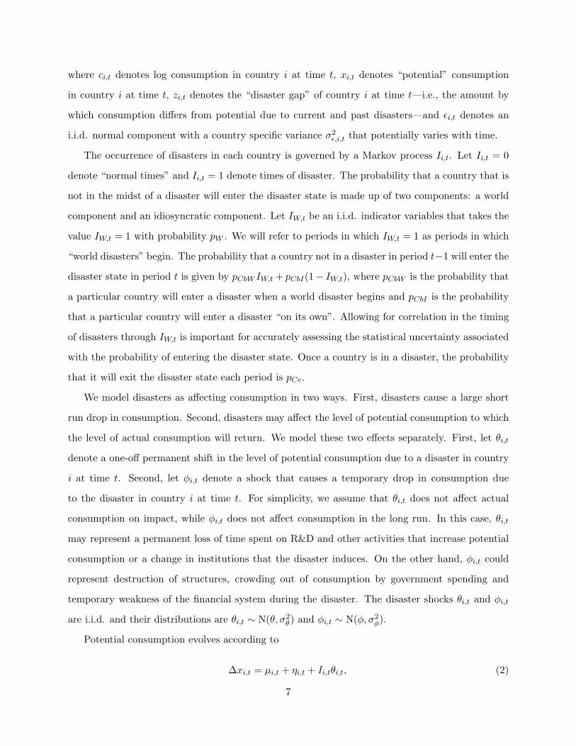
Figure 1 provides an illustration of a the type of disaster our model can generate. For simplicity,

we abstract from trend growth and set all other shocks than φi,t and θi,t to zero. The figure depicts

a disaster that lasts six periods and in which φi,t = −0.15 and θi,t = −0.05 in each period of the

disaster. Cumulatively, log consumption drops by roughly 0.67 from peak to trough. Consumption

then recovers substantially. In the long run, consumption is 0.30 lower than it was before the

disaster. This disaster is therefore partially permanent. The negative θi,t shocks during the disaster

permanently lower potential consumption. The fact that the shocks to φi,t are more negative than

the shocks to θi,t mean that consumption falls below potential consumption during the disaster.

The difference between potential consumption and actual consumption is the disaster gap in our

model. In the long run, the disaster gap closes—i.e., consumption recovers—so that only the drop

in potential consumption has a long run effect on consumption. Our model can generate a wide

range of disasters. If θi,t = 0 throughout the disaster, the entire disaster is transitory. If on the

other hand φi,t = θi,t throughout the disaster, the entire disaster is permanent.

A striking feature of the consumption data is the dramatic drop in volatility in many countries

following WWII. Part of this drop in consumption volatility likely reflects changes in the procedures

for constructing national accounts that were implemented at this time (Romer, 1986; Balke and

Gordon, 1989). We allow for this break by assumption that σ2ε,i,t and σ2

η,i,t each take two values

for each country: one before 1946 and one after. Another striking feature is that many countries

experienced very rapid growth for roughly 25 years after WWII. We allow for this by assuming that

8

µi,t takes three values for each country: one before 1946, one for the period 1946-1972 and one for

the period since 1973. The added flexibility that these assumptions yield dramatically improves

the fit of the model do the data. A drawback of modeling these features and one-time events is

that whatever generated these features of the data is not part of the process that will generate

future consumption in our model. While we have not investigated this issue formally, Bansal and

Yaron’s (2004) long-run risk model suggests that persistent movements in the average growth rate

of consumption could further raise the equity premium implied by our model.

One can show that the model is formally identified except for a few special cases in which

multiple shocks have zero variance. Nevertheless, the main challenge in estimating the model is the

relatively small number of disaster episodes observed in the data. Due to this scarcity of data on

disasters, we assume that all the disaster parameters—pW , pCbW , pCbI , pCe, ρz, θ, σ2θ , φ, σ2

φ—are

common across countries and time periods. This strong assumption allows us to pool information

about the disasters that have occurred in different countries and at different times. In contrast, we

allow that the non-disaster parameters—µi,t, σ2ε,i,t, σ

2η,i,t, σ

2ν,i—to vary across countries.

4 Estimation

The model presented in section 3 decomposes consumption into three unobserved components:

potential consumption, the disaster gap and a transitory shock. One way of viewing the model is,

thus, as disaster filter. Just as business cycle filters isolate movements in output attributable to

the business cycle, our model isolates movements in consumption that we attribute to disasters.

Maximum likelihood estimation of this model is difficult since it involves carrying out numerical

optimization over a high dimensional space of states and parameters. We instead use Bayesian

MCMC methods to estimate the model.7

7We sample from the posterior distributions of the parameters and states using a Gibbs sampler augmented withMetropolis steps when needed. This algorithm is described in greater detail in appendix A. The estimates discussedin section 5 are based on four independent Markov chains each with 1 million draws. The first 150,000 draws fromeach chain is dropped as burn-in. These chains are started from 2 different starting values, 2 chains from each startingvalue. We choose starting values that are far apart in the following way: The first set of starting values has Ii,t = 0for all i and all t and sets ci,t = xi,t and zi,t = 0 for all i and all t. The second set of starting values has Ii,t = 1 forall i and all t and sets xi,t equal to a smooth trend (with breaks in 1946 and 1973) and zi,t equal to consumptionminus this smooth trend. The first set of starting values thus attributes all the variation in the data to xi,t, whilethe second attributes all the variation in the data to zi,t. We use a number of techniques to assess convergence.First, we employ Gelman and Rubin’s (1992) approach to monitoring convergence based on parallel chains with“overdispersed starting points” (see also Gelman, et al. 2004, ch 11). Second, we calculate the “effective” samplesize (corrected for autocorrelation) for the parameters of the model. Finally, we visually evaluate “time series” plotsfrom our simulated Markow chains.

9

To carry out our Bayesian estimation we need to specify a set of priors on the parameters of the

model. To minimize the influence of the priors on our results, we specify relatively uninformative

priors for the majority of the parameters of the model. For a few parameters, however, we specify

informative priors. Our most important deviation from uninformative priors is that we assume that

disasters are rare and large. Specifically, we assume that pW ∼ Beta(1, 49), pCbI ∼ Beta(1, 49) and

φ ∼ N(−0.15, 0.007). One way to think of this assumption is that we are just defining disasters

to be events that are rare and give rise to large contractions in consumption in the short run.

Rietz (1988) and Barro (2006) show that large disasters are disproportionately important for asset

pricing. We are therefore disproportionately interested in accurately measuring disasters. Were we

not to define disasters to be rare and large but instead allow the model to use the zi,t process any

way it saw fit, it would tend to use zi,t to match high frequency features of the data that are not

particularly important for asset pricing. To avoid this, we force the model—through our choice of

informative priors—to use the zi,t process to capture only rare and large events.8

It is important to note that imposing informative priors on pW , pCbI and φ in no way ensures

that we will estimate disasters: the prior puts substantial weight on the model without disasters,

i.e. a model with pW = 0 and pCbI = 0. In fact, if we estimate our model on an artificial data set of

the same size as our data set simulated from a version of our model without disasters, the posterior

estimates of pW and pCbI are very close to zero (close enough that the model generates asset pricing

implications in line with Mehra and Prescott, 1985). Another point worth emphasizing is that we

do not assume an informative prior for θ—the mean of the long run disaster shock. We assume

that θ ∼ N(0, 0.22). Our prior on θ is agnostic about whether disasters have any long run effect at

all. Our estimated long run effect thus comes entirely from the data.

In addition, we restrict ρz to lie in the interval [0, 0.9]. Within this interval we assume that

ρz is uniformly distributed. These assumptions ensure that the half-life of the disaster gap is less

than 6.5 years. Again, we make these assumptions to ensure that the disasters generated by our

algorithm correspond to our intuitive notion of disasters. This assumptions on ρz rules out the

possibility that consumption growth in a given period can be explained by disasters that occurred

decades earlier.8An alternative prior that serves the same purpose is pW ∼ U(0, 0.05), pCbI ∼ U(0, 0.05). We have estimated

our model using this alternative prior for robustness. The results are quite similar. The main difference is that theposterior estimate of pW is somewhat higher and the equity premium is thus also somewhat higher. This is a naturalconsequence of the fact that this alternative prior has a higher mean for pW (0.025 rather than 0.02).

10

Finally, we restrict νi,t to be small. Specifically, we assume that σ2ν,i ∼ U(0, 0.0001). The

only reason we introduce νi,t at all to the disaster gap equation is to help our sampling algorithm

converge. We therefore restrict its magnitude such that it has a negligible effect on the predictions

of the model.9

The specific distributional assumptions we make for the remaining priors are in most cases

guided by a desire to have as many “conjugate” priors as possible since this improves the speed of

the numerical algorithm. Our choices for the remaining priors are:

σ2ε,i,t ∼ U(0, 0.152), σ2

η,i.t ∼ U(0, 0.152),

σ2ν,i.t ∼ U(0, 0.0001), µi,t ∼ N(0.02, 1),

pCbI ∼ U(0, 1), pCe ∼ U(0, 1),

1/σ2θ ∼ Gamma(10/3, 0.1/3), 1/σ2

φ ∼ Gamma(10/3, 0.1/3).

(4)

Given these assumptions we have a fully specified probability model for the evolution of consump-

tion.

5 Empirical Results

Table 1 presents our estimates of the disaster parameters, while tables 2–4 present our estimates

of µi,t, σε,i,t and ση,i,t, respectively. For each parameter, we present the assumed prior mean, prior

standard deviation and prior distribution, as well as the posterior mean and posterior standard

deviation. We refer to the posterior mean of each parameter as our point estimate of that parameter.

Consider first our estimates of the disaster parameters in table 1. We estimate the probability of

a world disaster to be 0.0194 per year. The probability that a world disaster will trigger a disaster in

a particular country is 0.5193. When the world is not in a disaster, the probability that a country

will enter a disaster “on its own” is 0.0043. The overall probability that a country will enter a

disaster is pW pCbW + (1− pW )pCbI . Since the three parameters involved are correlated, we cannot

simply multiply together the posterior mean estimates we have for them to get a posterior mean

of the overall probability of entering a disaster. Instead, we use the joint posterior distribution9MCMC algorithms have trouble converging when the objects one is estimating are highly correlated. In our case,

zt and zt+j for small j are highly correlated when there are no disturbances in the disaster gap equation betweentime t and time t+ j. This would be the case in the “no disaster” periods in our model if it did not include the νi,t

shock. In fact, zt and zt+j would be perfectly correlated in this case. It was in order to avoid this extremely highcorrelation that we introduced small disturbances to the disaster gap equation.

11

of these three parameters to calculate a posterior mean estimate of the overall probability that a

country enters a disaster. This yields and estimate for the overall probability of 0.0138. A centered

90% probability interval for this overall probability is [0.0064, 0.0231]. In contrast, a country that is

already in a disaster will continue to be in the disaster in the following year with a 0.833 probability.

This estimate implies that disasters last on average roughly six years.

Our estimate of ρz is 0.540. This implies that without further shocks about half of the disaster

gap dissipates each period. Our estimates of φ and σφ—the mean and standard deviation of φi,t—

are -0.134 and 0.110, respectively. The large negative estimate of φ is largely determined by the

informative prior we impose on this parameter. The large estimated value of σφ, however, gives us a

quantitative sense of the huge uncertainty associated with the short term evolution of consumption

during disasters.

Our estimates of θ and σθ—the mean and standard deviation of θi,t—are -0.025 and 0.105

respectively. This estimate of θ implies that disasters do on average have negative long run effects

on consumption. The fact that θ is estimated to be much smaller than φ, however, implies that

a large part of the effect of disasters on consumption in the short run is reversed in the long run.

The large estimate of σθ reveals that there is a huge amount of uncertainty during disasters about

the long run effect of the disaster on consumption as well as the short run effect of the disaster

on consumption. Taken together, these estimates put a substantial weight on the possibility of

extremely large negative shocks.

To get a better sense for what these parameters imply about the nature of consumption disasters,

figures 2 and 3 provide two different visual representations of the size of disasters and the extent

of recovery from disasters. Figure 2 plots the impulse response of an “typical disaster”. This is a

disaster than lasts for 6 years and the size of the short run effect and the long run effect are set

equal to the posterior mean of these parameters for each of the six disaster years (i.e. φi,t = φ and

θi,t = θ). It shows that the maximum short run effect of this typical disaster is approximately a

32% fall in consumption (a 0.38 fall in log consumption), while the long run negative effect of the

disaster is approximately 14%.

Figure 3 provides a slightly different view of disasters. Imagine an agent at time 1 who knows

that a disaster will begin at time 2 but knows nothing about the character of this disaster beyond the

unconditional distribution of disasters. The solid line in figure 3 plots the mean of the distribution

12

of beliefs of such an agent about the change in log consumption going forward upon receiving news

of the disaster. The dashed lines in the figure plot the median and 5% and 95% quantiles of this

same distribution. This figure therefore gives an ex ante view of disasters, while figure 2 gives an

ex post view of a particular disaster.

The shape of the solid line in figure 3 is quite different from the shape of the “typical” disaster

depicted in figure 2. In figure 3, the long run drop in the solid line is roughly 65% of the maximum

drop, while in figure 2 this ratio is only roughly 45%. This difference between the two figures arises

because, from the perspective of the agent standing at time 1, the distribution of the change in

consumption looking forward 10 or 15 years is highly skewed. On the one hand, most disasters

end within 6 years. On the other hand, if a disaster lasts beyond this, it is likely to be extremely

severe.10

Table 5 reports summary statistics for the main disaster episodes our model identifies. Our

Bayesian estimation procedure does not deliver a definitive judgement on whether a disaster oc-

curred at certain times and places but rather provides a posterior probability of whether a disaster

occurred. We must therefore define disaster episodes in some way. We define a disaster episode as

a set of consecutive years for a particular country such that: 1) The probability of a disaster in each

of these years is larger than 10%, and 2) The sum of the probability of disaster for each year over

the whole set of years is larger than one.11 Using this definition we identify 34 disaster episodes.

These episodes vary greatly in size and shape. On average, the maximum drop in consumption

due to the disasters is 33%. The permanent effect of disasters on consumption is on average 15%.

However, the largest short run effect of a disaster is a 60% drop in consumption in Japan during

WWII. Quite a few of the disaster episodes have huge long run effects. For example, we estimate

the long run effect of the disaster episode in Chile in the 1970’s and early 1980’s to be a 51% drop

in consumption relative to what would have occurred without the disaster, while the long run effect

of the Spanish Civil War and the subsequent turmoil was a 47% drop in consumption relative to

what would have occurred without the disaster.

The bulk of the disaster episodes we identify occur during World War I and World War II.10One way in which our model may understate the severity of disasters is that we assume that both φi,t and θi,t

have normal distributions. The fact that large negative events are much more frequent than large positive eventssuggests that perhaps a distribution with a fatter left tail than right tail may be more appropriate.

11More formally: A disaster episode is a set of consecutive years for a particular country, Ti, such that for all t ∈ Ti

P (Ii,t = 1) > 0.1 and∑

t∈TtP (Ii,t = 1) > 1.

13

Figure 4 plots our estimates of the probability that a “world disaster” began in each year.12 Our

model clearly identifies 1914 and 1940 as years in which world disasters began. In both of these

world wars, the model identifies a second year (1916 and 1943) in which these disasters seem to have

“intensified” and/or spread. In the case of WWII, 1943 marks a dramatic escalation of hostilities

in the Pacific theater. Apart from WWI and WWII, the model places a roughly 25% probability on

the Great Depression counting as a world disaster. The model identifies six disaster episodes that

are not associated with WWI and WWII. These include two of the most serious disaster episodes:

Spain during and after the Civil War and Chile during the early period of the reign of General

Pinochet. The U.S. Great Depression is identified as a disaster according to our model and so is

the Asian Financial Crisis in Korea.

Figure 5 provides more detail about how our model interprets the evolution of consumption

for France, Korea, Chile and the United States.13 The two lines in each panel plot consumption

and our estimate of potential consumption. The bars give our posterior probability estimate that

a country was in a disaster in each year. The left axis gives values of the probability of disaster,

while the right axis gives values for log consumption and potential consumption.

For France, the model picks up WWI and WWII as disasters. The model views WWII as largely

a transitory event for French consumption. The permanent effect of WWII on French consumption

is estimated to be only about 6%. The French experience in WWII is typical for many European

countries. For Korea, our model interprets the entire period from 1940 to 1954 as single long

disaster. This long disaster spans both WWII and the Korean War. In contrast to the experience

of many European countries, our estimates suggest that the crisis in the 1940’s and 1950’s had a

large permanent effect on Korean consumption (41%). This is typical of the experience of Asian

countries in our sample during WWII. For Korea, we also identify the Asian Financial Crisis as a

disaster.

Chile is one of the most volatile countries in our sample. Our model identifies two disaster

episodes for Chile. The first begins in WWI and spans the early years of the Great Depression.

The second disaster in Chile began in 1972 during the tenure of Salvator Allende but intensified

greatly in the early years of General Pinochet’s rule. The late 1970’s and early 1980’s are a period12This is the posterior mean of IW,t for each year. In other words, with the hindsight of all the data up until 2006,

what is our estimate of whether a world disaster began in say 1940?13More detailed figures for all the countries in our study are reported in a web appendix.

14

of recovery. But another period of huge declines in consumption starts in 1982 and lasts until

1987. This long disaster period is the most severe disaster we identify outside of periods of major

world wars. The last panel in figure 5 plots results for the United States. Relative to most other

countries in our sample, the United States was a tranquil place during our sample period. The Great

Depression is identified as a disaster. But it is a marginal disaster with the posterior probability

that a disaster occurred peaking at only about 30%.

According to our model, there have been no world disasters since the end of WWII. It is natural

to ask whether this provides evidence against the model. In fact, the rare nature of world disasters

implies that the posterior probability of experiencing no world disasters over a 62 year stretch

is roughly 30%. One could also ask whether the relative tranquility of the U.S. experience since

1890 provides evidence that the U.S. is fundamentally different than other countries in our sample.

However, the posterior probability for a single country experiencing no world disasters over a 117

year stretch is 19% according to our model. The posterior probability of at least one out of 24

countries experiencing no world disasters over a 117 year stretch is 88%. The tranquility of the

U.S. experience therefore does not provide evidence against our model.

Tables 2–4 present the remaining parameter estimates for our empirical model. Table 2 presents

country-specific estimates of the mean growth rate of potential consumption for the countries in our

sample. Recall that our model allows for breaks in the mean growth rate of potential consumption

in 1946 and 1973. We estimate sizable breaks of this kind both in 1946 and in 1973 for many

countries, especially those for which WWII was most disastrous. For example, we estimate that

the growth rate of potential consumption rose in Japan from 0.6% per year before 1946 to 7.5%

per year during 1946-1973 and then fell back to 2.2% per year after 1973. Similar, if somewhat

less extreme, changes in growth rates are estimated for Germany, France, Italy and many other

countries.14

Table 3 and 4 present country-specific estimates of the variance of both permanent and tran-

sitory shocks to consumption. We find a great deal of evidence that the stochastic properties of

consumption were different pre-1946 than they have been post-1946. For many countries, our esti-14If we do not allow for breaks in the mean growth rate, the model yields quite different results and a substantially

worse overall fit to the data. In this case, WWII is interpreted as having had a very large positive long run effectfor Japan, France and Italy (but a negative short run effect). The model interprets the rapid growth from 1946 to1973 as slow convergence to a much higher level of potential consumption. While this may be considered a plausiblealternative interpretation of the high growth between 1946-1973 in these countries, this specification of the modelyields less reasonable results for other countries and other periods contributing to its worse overall fit.

15

mates of the variance of both the permanent shocks to potential consumption and the transitory

shocks to consumption fell dramatically from the earlier period to the later period. This general

pattern is true for most of the original OECD members. A notable exception is the U.K. This

pattern of volatility reduction is also not as pronounced for the Latin American countries in our

sample.

6 Asset Pricing

We follow Mehra and Prescott (1985) in analyzing the asset pricing implications of the consumption

process we estimate above within the context of a representative consumer endowment economy.

We assume that the representative consumer in our model has preferences of the type developed by

Epstein and Zin (1989) and Weil (1990). For this preference specification, Epstein and Zin (1989)

show that the return on an arbitrary cash flow is given by the solution to the following equation:

Et

βξ (Ci,t+1

Ci,t

)(−ξ/ψ)

R−(1−ξ)w,t,t+1Ri,t,t+1

= 1, (5)

where Ri,t,t+1 denotes the gross return on an arbitrary asset in country i from period t to period

t + 1, Rw,t,t+1 denotes the gross return on the agent’s wealth, which in our model is equal to the

endowment stream. The parameter β represents the subjective discount factor of the representative

consumer. The parameter ξ = 1−γ1−1/ψ , where γ is the coefficient of relative risk aversion and ψ is

the intertemporal elasticity of substitution.15

Much work on asset pricing—including Mehra and Prescott (1985), Rietz (1988) and Barro

(2006)—considers the special case of power utility. In this case, γ = 1/ψ. A single parameter,

therefore governs both consumers’ willingness to bear risk, and their willingness to substitute

consumption over time. Bansal and Yaron (2004) and Barro (2009) among others have emphasized

the importance of delinking these two features of consumer preferences. Our results below provide

additional evidence in support of the more flexible model.

The asset pricing implications of our model with Epstein-Zin-Weil (EZW) preferences cannot be

derived analytically. We therefore use standard numerical methods. Initially, we calculate returns15The representative consumer approach we adopt abstracts from heterogeneity across consumers. Wilson (1968)

and Constantinides (1982) show that a heterogeneous consumer economy is isomorphic to a representative consumereconomy if markets are complete. See also Rubinstein (1974) and Caselli and Ventura (2000). Constantinides andDuffie (1996) argue that highly persistent, heteroscedastic uninsurable income shocks can resolve the equity premiumpuzzle.

16

for two assets: a one period risk-free bill and an unlevered claim on the consumption process. In

section 6.3, we calculate asset prices for a long term bond and allow for partial default on bills and

bonds during disasters.

Variation in the discount factor has only minimal effects on the equity premium in our model.16

It does however, affect the risk free rate. Given a calibration of γ and ψ, we can pick β to match

the risk free rate generated by the model to the risk free rate observed in the data. We set

β = exp(−0.035) to match the risk-free rate for our baseline specification. Mehra and Prescott

(1985) suggest that values for the coefficient of relative risk aversion below 10 are “reasonable”.

We consider a range of values in this reasonable range.

There is some debate in the macroeconomics and finance literature about the appropriate pa-

rameter value for the intertemporal elasticity of substitution (IES). Hall (1988) estimates the IES

to be close to zero. His estimates of the IES are obtained by analyzing the response of consumption

growth to movements in the interest rate over time. Yet, as noted by Bansal and Yaron (2004) and

Gruber (2006), such estimates are potentially subject to important endogeneity concerns. Both

the interest rate and consumption growth are the product of capital market equilibrium, making it

difficult to estimate the causal effect of one on the other. These concerns are sometimes addressed

by using lagged interest rates as instruments for movements in the current interest rate. However,

this instrumentation strategy is only successful if there are no slowly moving technology or prefer-

ence parameters that affect both interest rates and consumption growth. Alternative procedures

for identifying exogenous variation in the interest rate sometimes generate much larger estimates

of the IES. Gruber (2006) makes use of tax-based instruments for interest rates and estimates a

values close to 2 for the IES. As a consequence of this dispersion in empirical estimates, a wide

variety of parameter values for the IES are used in the asset pricing literature. On the one hand,

Campbell (2003) and Guvenen (2008) advocate values for the IES well below one, while Bansal

and Yaron (2004) use a value of the IES of 1.5 and Barro (2009) uses a value of 2. We argue below

that low values of the IES are starkly inconsistent with the observed behavior of asset prices during

consumption disasters. We will therefore focus on parameterizations with ψ = 2 as our baseline

case.

Barro and Ursua (2008) present data on rates of return for stocks and bonds for 17 countries16In the continuous time limit of our discrete time model, the equity premium is unaffected by β.

17

over a long sample period. The average arithmetic real rate of return on stocks in their data is

8.1% per year. The average arithmetic real rate of return on short term bills is 0.9% per year.

The average equity premium in their data is therefore roughly 7.2%. If we view stock returns as a

leveraged claim on the consumption stream, the target equity premium for an unlevered claim on

the consumption stream is lower than that for stocks. According to the Federal Reserve’s Flow-of-

Funds Accounts, the debt-equity ratio for U.S. non-financial corporations is roughly one-half. This

suggests that the target equity premium for our model should be 4.8% (7.2/1.5).17 We take this to

be our target.

The asset pricing results for our model are presented in table 6. We present results for both

the power utility case with γ = 1/ψ = 4 and also for EZW utility with ψ = 2 and a range of

values for γ. Our benchmark model based on the parameter values estimated in section 5 has

partially temporary disasters that unfold over multiple periods. To build intuition regarding which

features of the model are most important for generating a high equity premium, we also consider

two alternative specifications. First, we consider a version of our model in which the entire disaster

occurs in one period. In this case, we scale up the size of the disasters to make them roughly

comparable to the baseline case.18 Second, we consider a version of the model in which the disasters

are permanent on average.19 The statistics we report are the logarithm of the arithmetic average

gross return on each asset (logE[Ri,t,t+1]).

We present results on the one hand for a long sample with a representative set of disasters and

on the other hand for a long sample for which agents expect disasters to occur with their normal

frequency but no disasters actually occur. This latter case is meant to capture asset returns in

normal time such as the post-WWII period in OECD countries. Finally, we present results for a

version of the model in which we turn off the disasters completely. Without disasters, the model

generates an equity premium that is too small by a factor between 10 and 20. This is in line with

the results of Mehra and Prescott (1985).

In our analysis, we use the actual consumption data for the countries we study. These data17Dividing the equity premium for levered equity by one plus the dept-equity ratio to get a target for unlevered

equity is exactly appropriate in the simple disaster model of Barro (2006). Abel (1999) argues for approximatinglevered equity by a scaled consumption claim. Bansal and Yaron (2004) and others have adopted this approach. Forour model, these two approaches yield virtually indistinguishable results.

18The average duration of disasters in our baseline model is 5.98 years. When we consider single period disasters,we scale up φi,t by a factor of 1 + ρ+ ρ2 + ρ3 + ρ4 + 0.98ρ5, while we scale up θi,t by a factor of 5.98.

19Specifically, we raise the mean and standard deviation of θi,t to equal those of φi,t.

18

presumably reflect any international risk sharing that agents may have engaged in. The asset pricing

equations we use are standard Euler equations involving domestic consumption and domestic asset

returns. We could also investigate the asset pricing implications of Euler equations that link

domestic consumption, foreign consumption and the exchange rate (see, e.g., Backus and Smith,

1993). A large literature in international finance explores how the form that these Euler equations

take depends crucially on the structure of international financial markets. Analyzing these issues

is beyond the scope of this paper. However, recent work suggests that a time-varying probability

of rare disasters can help to explain anomalies in the behavior of the real exchange rate (Farhi and

Gabaix, 2008).

6.1 The Equity Premium with Power Utility

We begin by discussing the asset pricing implications of the simple power utility model with γ =

1/ψ = 4.20 For the baseline model with partially temporary multi-period disasters, the equity

premium is 1.4%. This is substantially less than the equity premium of 3.6% in Barro (2006).

However, a much more serious concern is that conditional on no disasters, the equity premium is

-0.3%, i.e., it is lower than in a model in which no disasters can happen. The overall equity premium

is, therefore, entirely coming from superior equity returns during disasters. This contrasts with the

results in Barro (2006) in which the equity premium arises in normal times and stocks do poorly

during disasters.

Why does our model with power utility yield such different results from earlier work by Barro

(2006)? The important difference is that disasters unfold over multiple periods in our model. A

version of our model with power utility and one period partially temporary disasters yields an equity

premium of 2.5% overall and 2.8% in normal times. To provide intuition about what generates these

results, figure 6 presents a time series plot of the behavior of equity and bond returns over the course

of a “typical” disaster, for our baseline model with power utility. Notice that there is a huge positive

return on equity at the start of the disaster (when the news arrives that a disaster has struck).

The reason for this large positive return is that entering the disaster state causes agents in

the model to expect further drops in consumption going forward. Since the agents in the model

have an IES equal to only 1/4 they have a tremendous desire to smooth consumption over time.20In this case, it is possible to solve for the return on the assets we consider analytically using an extension of the

calculations in Barro (2006).

19

This implies that they have a tremendous desire to save when they receive news that they are in a

disaster. This desire to save is so strong that it dominates the fact that entering a disaster is bad

news about the dividends of stocks. The disaster therefore causes a sharp rise in stock prices. In

contrast to stocks, the one period risk-free bond delivers a “normal” return in the first period of

the disaster. Together, these two facts imply that agents do not demand a high return for holding

stocks in normal times as a compensation for disaster risk. In contrast, stockholders demand a

large equity premium during disasters partly because they are scared that the disaster might end,

lowering the demand for assets and causing a sharp drop in stock prices.

Figure 7 presents a set of analogous results for the case of single period disasters with power

utility. The results for this case are much more intuitive. In this case, disasters occur instanta-

neously with no change in expected consumption growth going forward. As a consequence, there is

no increased desire to save pushing up stock prices. Equity, thus, fares extremely poorly relative to

bonds at the time of disasters and this generates a large equity premium in normal times. Needless

to say, the prediction of our multi-period disaster model with power utility that stocks yield hugely

positive returns at the onset of disasters is highly counterfactual. We take this as strong evidence

against low values of the IES at least during times of disaster.

6.2 The Equity Premium with Epstein-Zin-Weil Preferences

Given these counterfactual implications of the power utility model, we focus on asset pricing with

EZW preferences and an IES equal to 2. The asset pricing results from this specification are

presented in the lower half of table 6.21 Consider first the results for the baseline model with

partially temporary multi-period disasters. For γ = 7, the baseline model generates an equity

premium of 4.8%. Importantly, this case also generates a large equity premium in normal times.

The equity premium in the sample conditional on no disasters is also 4.8%. Furthermore, the mean

return on the risk-free bond is 1.0%, which is close to its value in the data. This specification

therefore generates both a large equity premium and a low risk-free rate with reasonable preference

parameters.21In this case, analytical computation of asset returns are not possible. We therefore employ a standard

numerical algorithm to solve the integral in equation (5) on a grid. Specifically, we rewrite equation (5) asPDRt = Et[f(∆Ct+1, PDRt+1)], where PDRt denotes the price dividend ratio of the asset in question, and solvenumerically for a fixed point for PDRt as a function of the state of the economy on a grid. This is a similar approachto the approach used by Campbell and Cochrane (1999) and Wachter (2008).

20

The results for the IES=2 case are much less sensitive to whether the disaster unfolds over

multiple periods or occurs in one period. This is a direct implication of the more moderate con-

sumption smoothing desire of agents with an IES of 2 than agents with an IES of 1/4. However, the

permanence of the disaster has a substantial effect on the size of the equity premium in the IES=2

case. The case with permanent disasters we consider in table 6 yields a very large equity premium

for modest values of risk aversion. The fact that we need to raise the value of risk aversion to seven

while Barro and Ursua (2008) can match the equity premium with a value of 3.5 is thus largely

due to the partially temporary nature of disasters in our model.

Figure 8 depicts equity and bond returns over the course of a “typical” disaster for the IES=2

case. The figure shows that the behavior of asset prices during a disaster is far more intuitive in this

case than in the case of power utility discussed above. Equity performs poorly relative to bonds at

the onset of the disaster, leading to an equity premium in normal times.

In a multi-period disaster in our model, much of the bad news associated with the disaster is

revealed at the start of the disaster—for example, at the start of a war. Stock market returns are

particularly low when this information is revealed. However, the low-point in consumption does not

occur until several years later. The low returns on equity during the disaster occur at a time when

consumption has just started to fall. In contrast, in the Barro-Rietz model, equity returns crash

precisely in the period when consumption has bottomed out and marginal utility is highest. This

feature of single-period disasters also contributes to a higher equity premium in the Barro-Rietz

model.

The asset pricing exercises discussed above are based on the posterior mean of the parameters

of our model. Given the limited amount of data we have to estimate the frequency, size and shape

of rare disasters, the posterior standard deviation of the parameters governing disasters are in

some cases substantial. Using the posterior distribution of the parameters of our model, we can

calculate a posterior distribution for the equity premium. This distribution is plotted in figure 9.

In calculating this distribution, we assume that agents have β = exp(−0.035), γ = 7 and ψ = 2.

Figure 9 shows that our estimates place a large weight on parameter combinations that generate a

significant equity premium. Parameter combinations that generate an equity premium of less than

2% get only roughly 5% weight. The centered 90% probability interval for the equity premium is

[0.020, 0.094].

21

To assess the degree to which our results on the equity premium are driven by the data as

opposed to our priors, we simulate an artificial dataset of the same size are our data (24 countries and

a total of 2685 observations) that contains no disasters. Specifically, we assume that consumption

follows a random walk with a mean growth rate of 2% per year and is hit by shocks that are

normally distributed with a standard deviation of 0.03. We then estimate our model on this data

and calculate the posterior distribution of the equity premium. This distribution is plotted in figure

10. For this alternative data set, our model places overwhelming probability (roughly 75%) on the

equity premium being below 1%. Clearly, our results would be very different if there in fact where

no disasters in the data. The distribution has a long right tail reflecting the fact that even a data

set the size of ours with no disasters would not entirely rule out the possibility that such events

could occur.

Figure 8 shows that the average return on bills are lower during disasters than they are during

normal times. Furthermore, returns on bills are temporarily high during the recovery periods after

disasters. These features of asset prices in our model line up well with the data. Barro (2006)

reports low returns on bills during many disasters. He also presents evidence that real returns

on U.S. Treasury bills have been unusually low during wars. This regularity is inconsistent with

many macroeconomic models (Barro, 1997, Ch. 12). There is furthermore some evidence that real

returns on bills is temporarily high after wars. This occurred in the U.S. after the Civil War and

after WWI.

One way to think about the importance of the features we have added relative to earlier work

on disasters is to ask how we could recalibrate the simpler model used in Barro and Ursua (2008)

to generate an equity premium of the same size as the equity premium our model yields. Recall

that in their model, all disasters are completely permanent. The appropriate parameters for the

model may, therefore, differ from the observed probability of (partially transient) disasters in the

data. The equity premium in Barro and Ursua (2008) is given by

logERe − logRf = γσ2 + pE{b[(1− b)−γ − 1]},

where p denotes the probability of disasters, b denotes the permanent instantaneous fraction by

which consumption drops at the time of disasters, σ2 denotes the variance of consumption growth in

normal times and γ denotes the coefficient of relative risk aversion. For simplicity, consider a version

of this model in which b is a constant. Barro and Ursua’s (2008) results can be roughly replicated

22

with p = 0.0363 and a constant size of disasters of b = 0.35. In contrast, the parameters of the

simple model with constant sized permanent disasters that match our results are p = 0.0138 and

b = 0.30. The substantially lower probability of disasters in our calibration—and the corresponding

lower equity premium for any given value of risk aversion—arises mainly from the fact that our

estimated model includes partial recoveries after many disasters.

6.3 Long Term Bonds, Inflation Risk and Partial Default

Our model generates variation in expected growth of consumption. This implies that the model

gives rise to a non-trivial term structure of interest rates. While one period bonds are risk-free,

the same is not true of longer term bonds. The return on long term bonds will reflect their risk

properties. Most long term government bonds promise a fixed set of payments in nominal terms.

Inflation risk will therefore affect the prices of these securities. Barro and Ursua (2008) present

data on long term bonds for 15 countries over a long sample period. These are nominal government

bonds usually of ten year maturity. The average arithmetic real rate of return in their data is

2.7% per year. The real return on bills for the same sample is 1.5% per year. The average real

term premium in their data is therefore 1.2% per year. To approximate such long bonds in our

model, we consider a perpetuity with coupon payments that decline over time. We denote the gross

annual growth rate of the coupon payments by Gp. We report results for Gp = 0.9 as this implies

a duration for our perpetuity that is similar to real-world ten year coupon bonds.22

The returns on such long term bonds are reported in table 7. The average return is -1.6% per

year. This implies a term premium of -2.6% per year. In contrast, the term premium in a version

of our model without disasters is virtually zero. The reason the long bond has such a low average

return in the presence of disasters is that it is an excellent hedge against disaster risk. To understand

why the long bond is a valuable hedge against disasters, it is useful to compare it to stocks. When

a disaster occurs, stocks are affected in two ways. First, the disaster is a negative shock to future

expected dividends. This effect tends to depress stock prices. Second, the representative consumer

has an increased desire to save. This tends to raise stock prices. With an IES=2, the first effect

dominates the second one and stocks decline at the beginning of a disaster. The difference between

a long term bond and stocks is that the coupon payments on the long term bonds are not affected22The duration of 10 year bonds with yields to maturity and coupon rates between 5% and 10% range from 6.5

years to 8 years. Our perpetuity has a duration of 7 years when it’s yield os 5%.

23

by the disaster. The only effect that the disaster has on the long term bond is therefore to raise

its price because of consumers’ increased desire the save. Since the price of long term bonds rises

at the onset of a disaster, long term bonds earn a lower rate of return than bills in normal times.

Barro and Ursua (2009) consider peak to trough drops in stock prices over time periods that

roughly correspond to consumption disasters. They note that in many cases large negative stock

returns occur slightly prior to or coincident with the consumption disasters. In some cases, however,

the timing of negative stock returns differs relative to the timing of the consumption disaster. They

argue that measurement issues can help explain this variation in timing and advocate a flexible

timing methodology.

Extending the asset price calculations of Barro and Ursua (2009) to bills, we find that in 73% of

the largest consumption disasters—22 cases out of 30—stock returns are lower than bill returns.23

The average stock return in these 22 cases is -38%, while the average bill return is -2%. In the

remaining 8 cases, the real return on stocks and bonds are similar. In these cases, the low real

returns on bills (and bonds) are caused by huge amounts of inflation. These cases also tend to be

ones in which the measurement of returns is most suspect because of market closure and controls

on goods and asset prices.

We follow Barro (2006) in calculating asset prices under the assumption that bills and bonds

experience partial default with certain probability during disasters due to large amounts of inflation.

Specifically, we assume that with some probability the return on bills and bonds is equal to the

return on equity. The calculations discussed above suggest that an appropriate calibration of the

probability of partial default is 27%. An earlier calculation by Barro (2006) based on somewhat less

extensive data suggests a probability of 40% for partial default. To be conservative, we consider

a case in which the probability of partial default is 40%. The last two columns of table 7 reports

results for this calibration. The partial default lowers the equity premium from 4.8% to 3.3%.

Raising the coefficient of risk aversion from 7 to 8 restores the equity premium to 4.7%. The

second column in table 7 reports results for a case in which the probability of partial default on

the perpetuity is 40%. This raises the average return on the perpetuity to -0.2% implying a term

premium of -1.1%. The third column considers a case in which the probability of partial default23We consider the subset of events in which the peak to trough drop in consumption is larger than 20%. This

yields a similar set of events to the disaster episodes in our model. For the subset of countries we use to estimate ourmodel, we get 35 events as compared to 34 disaster episodes identified by our model. There are 30 events for whichwe have data on both stock and bill returns.

24

is 70%. In this case, the return on the perpetuity is 2% and the term premium is 1.1%. In other

words, to match the term premium in the data, the perpetuity we consider need only provide

insurance against three of every 10 disasters.

7 Conclusion

In this paper, we estimate an empirical model of disasters building on the work of Rietz (1988),

Barro (2006) and Barro and Ursua (2008). The key innovations of our model are that we allow

disasters to be partly transitory, to unfold over multiple periods and for the timing of disasters

to be correlated across countries. Furthermore, we use a formal Bayesian estimation procedure

to match the data to the model. We find that it is possible to get into the right ballpark for

the observed equity premium using the estimated model, given “reasonable” values for the risk

aversion of the representative consumer. The degree of risk aversion we need to assume to match

the empirical equity premium is higher than in Barro (2006) and Barro and Ursua (2008) mainly

because we estimate substantial recoveries after disasters. Our asset pricing results depend crucially

on the assumption that the coefficient of relative risk aversion and the intertemporal elasticity of

substitution may be disentangled from the as in the Epstein-Zin-Weil specification of preferences

so that both of these parameters can take values above one. With an interpemporal elasticity

of substitution substantially below one, our asset pricing model counterfactually generates stock

market booms at the onset of disasters.

25

A Model Estimation

We employ a Bayesian MCMC algorithm to estimate our model. More specifically, we employ

a Metropolized Gibbs sampling algorithm to sample from the joint posterior distribution of the

unknown parameters and variables conditional on the data. This algorithm takes the following

form in the case of our model.

The full probability model we employ may be denoted by

f(Y,X,Θ) = f(Y,X|Θ)f(Θ),

where Y ∈ {Ci,t} is the set of observable variables for which we have data,

X ∈ {xi,t, zi,t, IW,t, Ii,t, φi,t, θi,t}

is the set of unobservable variables,

Θ ∈ {pW , pCbW , pCbI , pCe, ρz, θ, σ2θ , φ, σ

2φ, µi, σ

2ε,i, σ

2η,i, σ

2ν,i}

is the set of parameters. From a Bayesian perspective, there is no real importance to the distinction

between X and Θ. The only important distinction is between variables that are observed and

those that are not. The function f(Y,X|Θ) is often referred to as the likelihood function of the

model, while f(Θ) is often referred to as the prior distribution. Both f(Y,X|Θ) and f(Θ) are

fully specified in sections 3 and 4 of the paper. The likelihood function may be constructed by

combining equations (1)-(3), the distributional assumptions for the shocks in these equations and

the distributional assumptions made about Ii,t and IW,t in section 3. The prior distribution is

described in detail in section 4.

The object of interest in our study is the distribution f(X,Θ|Y ), i.e., the joint distribution of

the unobservables conditional on the observed values of the observables. For expositional simplicity,

let Φ = (X,Θ). Using this notation, the object of interest is f(Φ|Y ). The Gibbs sampler algorithm

produces a sample from the joint distribution by breaking the vector of unknown variables into

subsets and sampling each subvector sequentially conditional on the value of all the other unknown

variables (see, e.g., Gelman et al., 2004, and Geweke, 2005). In our case we implement the Gibbs

sampler as follows.

1. We derive the conditional distribution of each element of Φ conditional on all the other

elements and conditional on the observables. For the ith element of Φ, we can denote this

26

conditional distribution as f(Φi|Φ−i, Y ), where Φi denotes the ith element of Φ and Φ−i

denotes all but the ith element of Φ. In most cases, f(Φi|Φ−i, Y ) are common distributions

such as normal distributions or gamma distributions for which samples can be drawn in a

computationally efficient manner. For example, the distribution of potential consumption for

a particular country in a particular year, xi,t, conditional on all other variables is normal.

This makes using the Gibbs sampler particularly efficient in our application. Only in a few

cases (ρz, σ2ε,i, σ

2η,i, σ

2ν,i) are the conditional distributions not readily recognizable. In these

cases, we use the Metropolis algorithm to sample values of f(Φi|Φ−i, Y ).24

2. We propose initial values for all the unknown variables Φ. Let Φ0 denote these initial values.

3. We cycle through Φ sampling Φti from the distribution f(Φi|Φt−1

−i , Y ) where

Φt−1−i = (Φt

1, ...,Φti−1,Φ

t−1i+1, ...,Φ

t−1d )

and d denotes the number of elements in Φ. At the end of each cycle, we have a new draw

Φt. We repeat this step N times to get a sample of N draws for Φ.

4. It has been shown that samples drawn in this way converge to the distribution f(Φ|Y ) under

very general conditions (see, e.g., Geweke, 2005). We assess convergence and throw away an

appropriate burn-in sample.

In practice, we run four such “chains” starting two from one set of initial values and two from

another set of initial values. We run each chain for 1 million draws and throw away the first 150,000

draws for each chain. Given a sample from the joint distribution f(Φ|Y ) of the unobserved variables

conditional on the observed data, we can calculate any statistic of interest that involves Φ. For

example, we can calculate the mean of any element of Φ by calculating the sample analogue of the

integral ∫Φif(Φi|Φt−1

−i , Y )dΦi.

24The Metropolis algorithm samples a proposal Φ∗i from a proposal distribution Jt(Φ∗i |Φt−1

i ). This proposal dis-tribution must by symmetric, i.e., Jt(xa|xb) = Jt(xb|xa). The proposal is accepted with probability min(r, 1) wherer = f(Φ∗i |Φ−i, Y )/f(Φt−1

i |Φ−i, Y ). If the proposal is accepted, Φti = Φ∗i . Otherwise Φt

i = Φt−1i . Using the Metropolis

algorithm to sample from f(Φi|Φ−i, Y ) is much less efficient than the standard algorithms used to sample from knowndistributions such as the normal distribution in most software packages. Intuitively, this is because it is difficult tocome up with an efficient proposal distribution. The proposal distribution we use is a normal distribution centeredat Φt−1

i .

27

References

Abel, A. B. (1999): “Risk Premia and Term premia in General Equilibrium,” Journal of MonetaryEconomics, 43, 3–33.

Backus, D. K., and G. W. Smith (1993): “Consumption and Real Exchange Rates in DynamicEconomcies with Non-Traded Goods,” Journal of International Economics, 35(3-4), 297–316.

Balke, N. S., and R. J. Gordon (1989): “The Estimation of Prewar Gross National Product:Methodology and New Evidence,” Journal of Political Economics, 97, 38–92.

Bansal, R., and A. Yaron (2004): “Risks for the Long Run: A Potential Resolution of AssetPricing Puzzles,” Journal of Finance, 59(4), 1481–1509.

Barro, R. (1997): Macroeconomics. MIT Press, Cambridge, MA.

(2006): “Rare Disasters and Asset Markets in the Twentieth Century,” Quarterly Journalof Economics, 121(3), 832–866.

(2009): “Rare Disasters, Asset Prices, and Welfare Costs,” American Economic Review,99(1), 243–264.

Barro, R. J., and J. F. Ursua (2008): “Macroeconomic Crises since 1870,” Brookings Paperson Economic Activity, 2008, 255–350.

(2009): “Stock-Market Crashes and Depressions,” NBER Working Paper No. 14760.

Campbell, J. Y. (2003): “Consumption-Based Asset Pricing,” in Handbook of the Economics ofFinance, ed. by G. Constantinides, M. Harris, and R. Stulz, pp. 804–887, Amsterdam. Elsevier.

Campbell, J. Y., and J. H. Cochrane (1999): “By force of habit: A consumption-basedexplanation of aggregate stock market behavior,” Journal of Political Economics, Journal ofPolitical Economics(107), 205–251.

Caselli, F., and J. Ventura (2000): “A Representative Consumer Theory of Distribution,”American Economic Review, 90, 909–926.

Cochrane, J. H. (1988): “How Big Is the Random Walk in GNP?,” Journal of Political Eco-nomics, 96(5), 893–920.

Cogley, T. (1990): “International Evidence on the Size of the Random Walk in Output,” Journalof Political Economics, 98(3), 501–518.

Constantinides, G. (1982): “Intertemporal Asset Pricing with Heterogeneous Consumers andwithout Demand Aggregation,” Journal of Business, 55(2), 253–267.

(2008): “Consumption Crises since 1870,” Brookings Conference Discussion of “Macroe-conomic Crises since 1870” by Robert J. Barro and Jose F. Ursua.

Constantinides, G., and D. Duffie (1996): “Asset Pricing with heterogeneous consumers,”Journal of Political Economics, 104(2), 219–240.

28

Dimson, E., P. Marsh, and M. Staunton (2002): Triumph of the Optimists. Princeton Uni-versity Press, Princeton, New Jersey.

Epstein, L. G., and S. E. Zin (1989): “Substitution, Risk Aversion and the Temporal Behaviorof Consumption and Asset Returns,” Econometrica, 57, 937–969.

Farhi, E., and X. Gabaix (2008): “Rare Disasters and Exchange Rates,” Working Paper.

Gabaix, X. (2008): “Variable Rare Disasters: A Tractable Theory of Ten Puzzles in Macro-Finance,” American Economic Review, 98(2), 64–67.

Gelfand, A. (2000): “Gibbs Sampling,” Journal of the American Statistical Association, 95(452),1300–1304.

Gelman, A., J. B. Carlin, H. S. Stern, and D. B. Rubin (2004): Bayesian Data Analysis.John Wiley and Sons, Hoboken, New Jersey.

Gelman, A., and D. B. Rubin (1992): “Inference from Iterative Simulation Using MultipleSequences,” Statistical Science, 7, 457–511.

Geweke, J. (2005): Contemporary Bayesian Econometrics and Statistics. Chapman & Hall/CRC,Boca Raton, Florida.

Gourio, F. (2008): “Disasters and Recoveries,” American Economic Review, 98(2), 68–73.

Gruber, J. (2006): “A Tax-Based Estimate of the Elasticity of Intertemporal Substitution,”NBER Working Paper No. 11945.

Guvenen, F. (2008): “A Parsimonious Macroeconomic Model for Asset Pricing,” Working Paper.

Hall, R. E. (1988): “Intertemporal Substitution in Consumption,” Journal of Political Economics,96(2), 339–357.

Julliard, C., and A. Ghosh (2008): “Can Rare Events Explain the Equity Premium Puzzle?,”Working Paper.

Lucas, R. E. (1978): “Asset Prices in an Exchange Economy,” Econometrica, 46(6), 1429–1445.

Maddison, A. (2003): The World Economy: Historical Statistics. OECD, Paris.

Martin, I. (2008): “Disasters and the Welfare Cost of Uncertainty,” American Economic Review,98(2), 74–78.

Mehra, R., and E. C. Prescott (1985): “The Equity Premium: A Puzzle,” Journal of MonetaryEconomics, 15, 145–161.

Rietz, T. A. (1988): “The Equity Risk Premium: A Solution,” Journal of Monetary Economics,22, 117–131.

Romer, C. D. (1986): “Is the Stabilization of the Postwar Economy a Figment of the Data,”American Economic Review, 1986(76), 314–334.

Rubinstein, M. (1974): “An Aggregation Theorem for Securities Markets,” Journal of FinancialEconomics, 1, 225–244.

29

Smith, A., and A. Gelfand (1992): “Bayesian Statistics without Tears: A Sampling-ResamplingPerspective,” The American Statistician, 46(2), 84–88.

Wachter, J. A. (2008): “Can time-varying risk of rare disasters explain aggregate stock marketvolatility,” Working Paper.

Weil, P. (1990): “Nonexpected Utility in Macroeconomics,” Quarterly Journal of Economics,105(1), 29–42.

Wilson, R. B. (1968): “The Theory of Syndicates,” Econometrica, 36, 119–132.

30

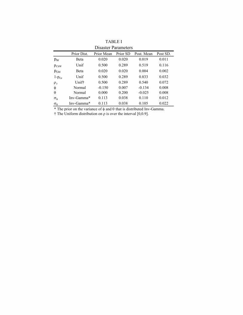
Prior Dist. Prior Mean Prior SD Post. Mean Post SD.pW Beta 0.020 0.020 0.019 0.011pCbW Unif 0.500 0.289 0.519 0.116pCbI Beta 0.020 0.020 0.004 0.0021-pCe Unif 0.500 0.289 0.833 0.032ρz Unif† 0.500 0.289 0.540 0.072φ Normal -0.150 0.007 -0.134 0.008θ Normal 0.000 0.200 -0.025 0.008σφ Inv-Gamma* 0.113 0.038 0.110 0.012σθ Inv-Gamma* 0.113 0.038 0.105 0.022

TABLE IDisaster Parameters

* The prior on the variance of φ and θ that is distributed Inv-Gamma.† The Uniform distribution on ρ is over the interval [0,0.9].

Prior Dist. Prior Mean Prior SD Post. Mean Post SD. Post. Mean Post SD. Post. Mean Post SD.Argentina Normal 0.02 1.00 0.013 0.009 0.018 0.011 0.007 0.010Australia Normal 0.02 1.00 0.008 0.010 0.021 0.005 0.020 0.003Belgium Normal 0.02 1.00 0.007 0.008 0.027 0.005 0.019 0.003Brazil Normal 0.02 1.00 0.022 0.010 0.038 0.010 0.017 0.008Canada Normal 0.02 1.00 0.020 0.009 0.025 0.004 0.018 0.004Chile Normal 0.02 1.00 0.017 0.010 0.024 0.009 0.037 0.011Denmark Normal 0.02 1.00 0.018 0.003 0.021 0.005 0.012 0.004Finland Normal 0.02 1.00 0.021 0.008 0.042 0.007 0.023 0.006France Normal 0.02 1.00 0.004 0.004 0.037 0.003 0.019 0.002Germany Normal 0.02 1.00 0.011 0.005 0.050 0.004 0.018 0.003Italy Normal 0.02 1.00 0.008 0.003 0.046 0.004 0.021 0.003Japan Normal 0.02 1.00 0.006 0.005 0.075 0.005 0.022 0.003Korea Normal 0.02 1.00 0.016 0.005 0.033 0.008 0.050 0.006Mexico Normal 0.02 1.00 0.006 0.010 0.025 0.007 0.015 0.006Netherlands Normal 0.02 1.00 0.011 0.005 0.034 0.007 0.015 0.004Norway Normal 0.02 1.00 0.013 0.004 0.028 0.004 0.025 0.004Peru Normal 0.02 1.00 0.019 0.006 0.031 0.007 0.008 0.008Portugal Normal 0.02 1.00 0.012 0.010 0.042 0.007 0.030 0.006Spain Normal 0.02 1.00 0.009 0.007 0.054 0.008 0.021 0.004Sweden Normal 0.02 1.00 0.026 0.004 0.025 0.005 0.013 0.003Switzerland Normal 0.02 1.00 0.013 0.005 0.027 0.003 0.009 0.002Taiwan Normal 0.02 1.00 0.004 0.010 0.056 0.008 0.055 0.006U.K. Normal 0.02 1.00 0.010 0.002 0.020 0.004 0.024 0.004U.S. Normal 0.02 1.00 0.013 0.006 0.025 0.003 0.022 0.003

Median 0.012 0.006 0.029 0.005 0.019 0.004Simple Average 0.013 0.007 0.034 0.006 0.022 0.005

Post-1973

Mean Growth Rate of Potential ConsumptionTABLE II

Prior Pre-1946 1946-1972

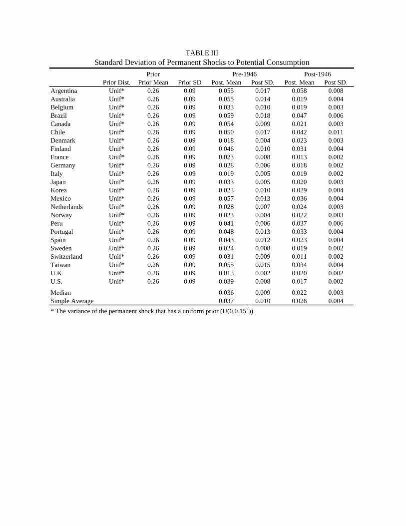
Prior Dist. Prior Mean Prior SD Post. Mean Post SD. Post. Mean Post SD.Argentina Unif* 0.26 0.09 0.055 0.017 0.058 0.008Australia Unif* 0.26 0.09 0.055 0.014 0.019 0.004Belgium Unif* 0.26 0.09 0.033 0.010 0.019 0.003Brazil Unif* 0.26 0.09 0.059 0.018 0.047 0.006Canada Unif* 0.26 0.09 0.054 0.009 0.021 0.003Chile Unif* 0.26 0.09 0.050 0.017 0.042 0.011Denmark Unif* 0.26 0.09 0.018 0.004 0.023 0.003Finland Unif* 0.26 0.09 0.046 0.010 0.031 0.004France Unif* 0.26 0.09 0.023 0.008 0.013 0.002Germany Unif* 0.26 0.09 0.028 0.006 0.018 0.002Italy Unif* 0.26 0.09 0.019 0.005 0.019 0.002Japan Unif* 0.26 0.09 0.033 0.005 0.020 0.003Korea Unif* 0.26 0.09 0.023 0.010 0.029 0.004Mexico Unif* 0.26 0.09 0.057 0.013 0.036 0.004Netherlands Unif* 0.26 0.09 0.028 0.007 0.024 0.003Norway Unif* 0.26 0.09 0.023 0.004 0.022 0.003Peru Unif* 0.26 0.09 0.041 0.006 0.037 0.006Portugal Unif* 0.26 0.09 0.048 0.013 0.033 0.004Spain Unif* 0.26 0.09 0.043 0.012 0.023 0.004Sweden Unif* 0.26 0.09 0.024 0.008 0.019 0.002Switzerland Unif* 0.26 0.09 0.031 0.009 0.011 0.002Taiwan Unif* 0.26 0.09 0.055 0.015 0.034 0.004U.K. Unif* 0.26 0.09 0.013 0.002 0.020 0.002U.S. Unif* 0.26 0.09 0.039 0.008 0.017 0.002

Median 0.036 0.009 0.022 0.003Simple Average 0.037 0.010 0.026 0.004* The variance of the permanent shock that has a uniform prior (U(0,0.152)).

Prior Pre-1946 Post-1946

TABLE IIIStandard Deviation of Permanent Shocks to Potential Consumption

Prior Dist. Prior Mean Prior SD Post. Mean Post SD. Post. Mean Post SD.Argentina Unif* 0.26 0.09 0.039 0.019 0.017 0.008Australia Unif* 0.26 0.09 0.023 0.010 0.005 0.003Belgium Unif* 0.26 0.09 0.012 0.007 0.005 0.002Brazil Unif* 0.26 0.09 0.059 0.014 0.015 0.007Canada Unif* 0.26 0.09 0.018 0.008 0.005 0.002Chile Unif* 0.26 0.09 0.038 0.017 0.022 0.009Denmark Unif* 0.26 0.09 0.009 0.004 0.007 0.003Finland Unif* 0.26 0.09 0.016 0.008 0.006 0.004France Unif* 0.26 0.09 0.029 0.005 0.003 0.001Germany Unif* 0.26 0.09 0.011 0.006 0.003 0.002Italy Unif* 0.26 0.09 0.012 0.004 0.004 0.002Japan Unif* 0.26 0.09 0.012 0.005 0.005 0.003Korea Unif* 0.26 0.09 0.029 0.007 0.006 0.003Mexico Unif* 0.26 0.09 0.027 0.011 0.008 0.004Netherlands Unif* 0.26 0.09 0.016 0.007 0.004 0.002Norway Unif* 0.26 0.09 0.006 0.003 0.006 0.003Peru Unif* 0.26 0.09 0.011 0.006 0.007 0.004Portugal Unif* 0.26 0.09 0.020 0.010 0.007 0.004Spain Unif* 0.26 0.09 0.040 0.009 0.005 0.003Sweden Unif* 0.26 0.09 0.018 0.007 0.004 0.002Switzerland Unif* 0.26 0.09 0.033 0.007 0.002 0.001Taiwan Unif* 0.26 0.09 0.033 0.015 0.006 0.003U.K. Unif* 0.26 0.09 0.005 0.002 0.004 0.002U.S. Unif* 0.26 0.09 0.019 0.006 0.004 0.002

Median 0.018 0.007 0.005 0.003Simple Average 0.022 0.008 0.007 0.003* The variance of the permanent shock that has a uniform prior (U(0,0.152)).

TABLE IV

Prior Pre-1946 Post-1946

Standard Deviation of Temporary Shock to Consumption

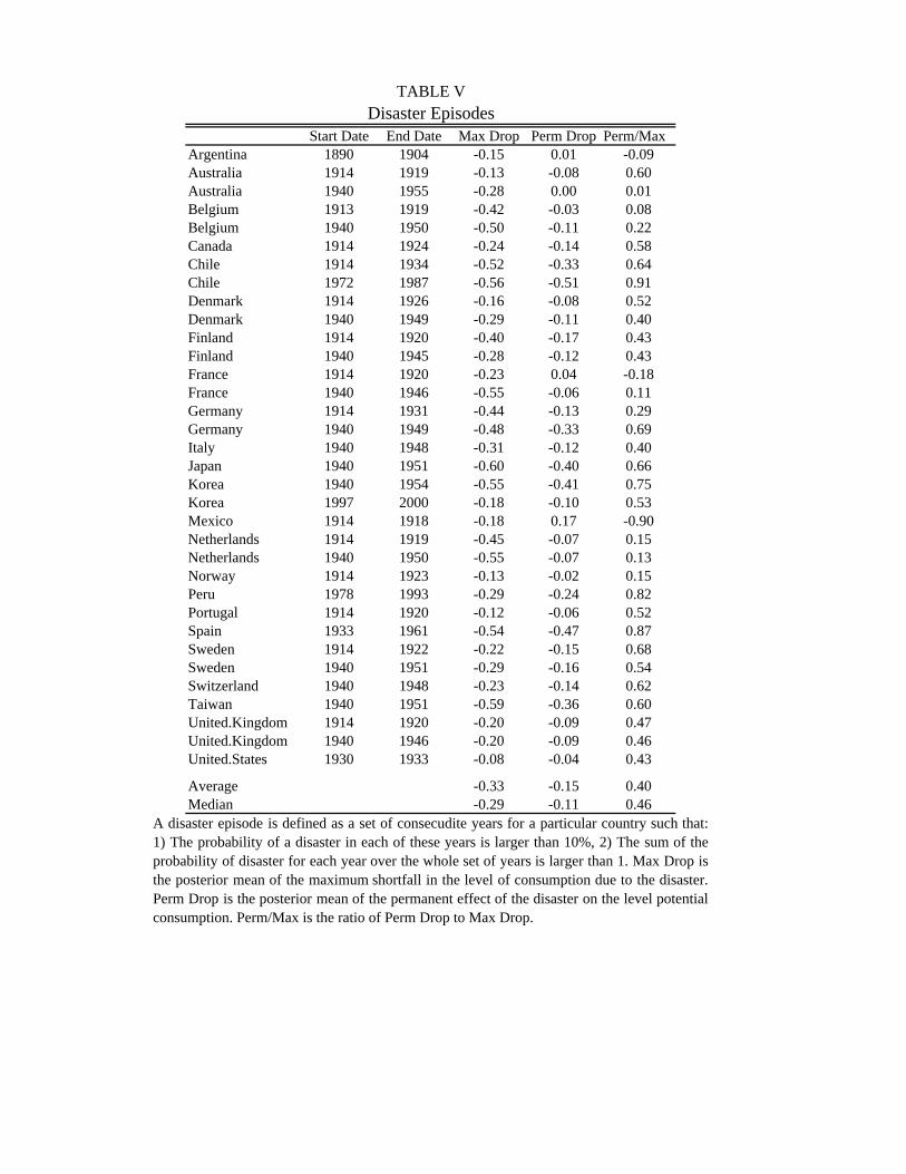
Start Date End Date Max Drop Perm Drop Perm/MaxArgentina 1890 1904 -0.15 0.01 -0.09Australia 1914 1919 -0.13 -0.08 0.60Australia 1940 1955 -0.28 0.00 0.01Belgium 1913 1919 -0.42 -0.03 0.08Belgium 1940 1950 -0.50 -0.11 0.22Canada 1914 1924 -0.24 -0.14 0.58Chile 1914 1934 -0.52 -0.33 0.64Chile 1972 1987 -0.56 -0.51 0.91Denmark 1914 1926 -0.16 -0.08 0.52Denmark 1940 1949 -0.29 -0.11 0.40Finland 1914 1920 -0.40 -0.17 0.43Finland 1940 1945 -0.28 -0.12 0.43France 1914 1920 -0.23 0.04 -0.18France 1940 1946 -0.55 -0.06 0.11Germany 1914 1931 -0.44 -0.13 0.29Germany 1940 1949 -0.48 -0.33 0.69Italy 1940 1948 -0.31 -0.12 0.40Japan 1940 1951 -0.60 -0.40 0.66Korea 1940 1954 -0.55 -0.41 0.75Korea 1997 2000 -0.18 -0.10 0.53Mexico 1914 1918 -0.18 0.17 -0.90Netherlands 1914 1919 -0.45 -0.07 0.15Netherlands 1940 1950 -0.55 -0.07 0.13Norway 1914 1923 -0.13 -0.02 0.15Peru 1978 1993 -0.29 -0.24 0.82Portugal 1914 1920 -0.12 -0.06 0.52Spain 1933 1961 -0.54 -0.47 0.87Sweden 1914 1922 -0.22 -0.15 0.68Sweden 1940 1951 -0.29 -0.16 0.54Switzerland 1940 1948 -0.23 -0.14 0.62Taiwan 1940 1951 -0.59 -0.36 0.60United.Kingdom 1914 1920 -0.20 -0.09 0.47United.Kingdom 1940 1946 -0.20 -0.09 0.46United.States 1930 1933 -0.08 -0.04 0.43

Average -0.33 -0.15 0.40Median -0.29 -0.11 0.46

Disaster EpisodesTABLE V

A disaster episode is defined as a set of consecudite years for a particular country such that:1) The probability of a disaster in each of these years is larger than 10%, 2) The sum of theprobability of disaster for each year over the whole set of years is larger than 1. Max Drop isthe posterior mean of the maximum shortfall in the level of consumption due to the disaster.Perm Drop is the posterior mean of the permanent effect of the disaster on the level potentialconsumption. Perm/Max is the ratio of Perm Drop to Max Drop.

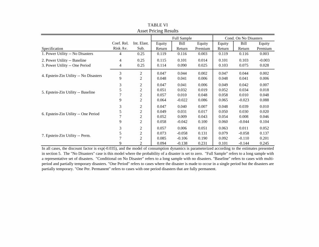
SpecificationEquity Return

Bill Return

Equity Premium

Equity Return

Bill Return

Equity Premium

1. Power Utility -- No Disasters 4 0.25 0.119 0.116 0.003 0.119 0.116 0.0032. Power Utility -- Baseline 4 0.25 0.115 0.101 0.014 0.101 0.103 -0.0033. Power Utility -- One Period 4 0.25 0.114 0.090 0.025 0.103 0.075 0.028

3 2 0.047 0.044 0.002 0.047 0.044 0.0029 2 0.048 0.041 0.006 0.048 0.041 0.0063 2 0.047 0.041 0.006 0.049 0.042 0.0075 2 0.051 0.032 0.019 0.052 0.034 0.0187 2 0.057 0.010 0.048 0.058 0.010 0.0489 2 0.064 -0.022 0.086 0.065 -0.023 0.0883 2 0.047 0.040 0.007 0.048 0.039 0.0105 2 0.049 0.031 0.017 0.050 0.030 0.0207 2 0.052 0.009 0.043 0.054 0.008 0.0469 2 0.058 -0.042 0.100 0.060 -0.044 0.1043 2 0.057 0.006 0.051 0.063 0.011 0.0525 2 0.073 -0.058 0.131 0.079 -0.058 0.1377 2 0.085 -0.106 0.190 0.092 -0.110 0.2019 2 0.094 -0.138 0.231 0.101 -0.144 0.245

TABLE VIAsset Pricing Results

4. Epstein-Zin Utility -- No Disasters

5. Epstein-Zin Utility -- Baseline

Coef. Rel. Risk Av.

Int. Elast. Sub.

6. Epstein-Zin Utility -- One Period

7. Epstein-Zin Utility -- Perm.

Full Sample Cond. On No Disasters

In all cases, the discount factor is exp(-0.035), and the model of consumption dynamics is parameterized according to the estimates presentedin section 5. The "No Disasters" case is this model where the probability of a disaster is set to zero. "Full Sample" refers to a long sample witha representative set of disasters. "Conditional on No Disaster" refers to a long sample with no disasters. "Baseline" refers to cases with multi-period and partially temporary disasters. "One Period" refers to cases where the disaster is made to occur in a single period but the disasters arepartially temporary. "One Per. Permanent" refers to cases with one period disasters that are fully permanent.

(1) (2) (3) (4) (5)Coefficient of relative risk aversion 7 7 7 7 8Intertemporal elasticity of substitution 2 2 2 2 2Rate of time preference 0.035 0.035 0.035 0.035 0.035

Dividend growth for perpetuity 0.9 0.9 0.9 0.9 0.9Probability of partial default on perpetuity 0.0 0.4 0.7 0.4 0.4Probability of partial default on one period bond 0.0 0.0 0.0 0.4 0.4

Log expected return on equity 0.057 0.057 0.057 0.057 0.061Log expected return on one period bond 0.010 0.010 0.010 0.024 0.014Log expected return on perpetuity -0.016 -0.002 0.020 -0.002 -0.017

Equity premium 0.048 0.048 0.048 0.033 0.047Term premium -0.026 -0.011 0.011 -0.026 -0.031

Average duration of perpetuity in normal times 10.6 9.2 7.7 9.2 10.7

TABLE VIILong Term Bonds and Parial Default

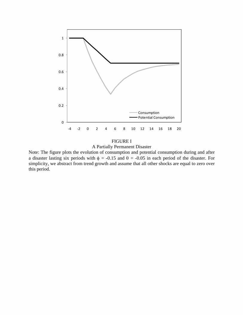
FIGURE I

A Partially Permanent Disaster Note: The figure plots the evolution of consumption and potential consumption during and after a disaster lasting six periods with φ = -0.15 and θ = -0.05 in each period of the disaster. For simplicity, we abstract from trend growth and assume that all other shocks are equal to zero over this period.

0

0.2

0.4

0.6

0.8

1

‐4 ‐2 0 2 4 6 8 10 12 14 16 18 20

ConsumptionPotential Consumption

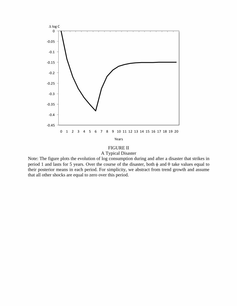
FIGURE II

A Typical Disaster Note: The figure plots the evolution of log consumption during and after a disaster that strikes in period 1 and lasts for 5 years. Over the course of the disaster, both φ and θ take values equal to their posterior means in each period. For simplicity, we abstract from trend growth and assume that all other shocks are equal to zero over this period.

‐0.45

‐0.4

‐0.35

‐0.3

‐0.25

‐0.2

‐0.15

‐0.1

‐0.05

0

0 1 2 3 4 5 6 7 8 9 10 11 12 13 14 15 16 17 18 19 20

Δ log C

Years

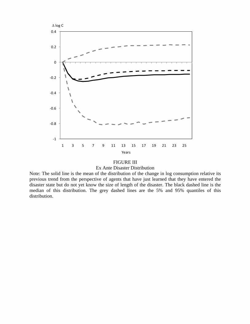
FIGURE III Ex Ante Disaster Distribution

Note: The solid line is the mean of the distribution of the change in log consumption relative its previous trend from the perspective of agents that have just learned that they have entered the disaster state but do not yet know the size of length of the disaster. The black dashed line is the median of this distribution. The grey dashed lines are the 5% and 95% quantiles of this distribution.

‐1

‐0.8

‐0.6

‐0.4

‐0.2

0

0.2

0.4

1 3 5 7 9 11 13 15 17 19 21 23 25

Δ log C

Years

FIGURE IV World Disaster Probability

Note: The figure plots the posterior mean of IW,t, i.e., the probability that the world entered a disaster in each year evaluated using data up to 2006.

0

0.1

0.2

0.3

0.4

0.5

0.6

0.7

0.8

0.9

1

1890 1900 1910 1920 1930 1940 1950 1960 1970 1980 1990 2000

1900 1920 1940 1960 1980 2000

0.0

0.4

0.8

France

Year

2.5

3.5

4.5

1920 1940 1960 1980 2000

0.0

0.4

0.8

Korea

Year

2.0

3.0

4.0

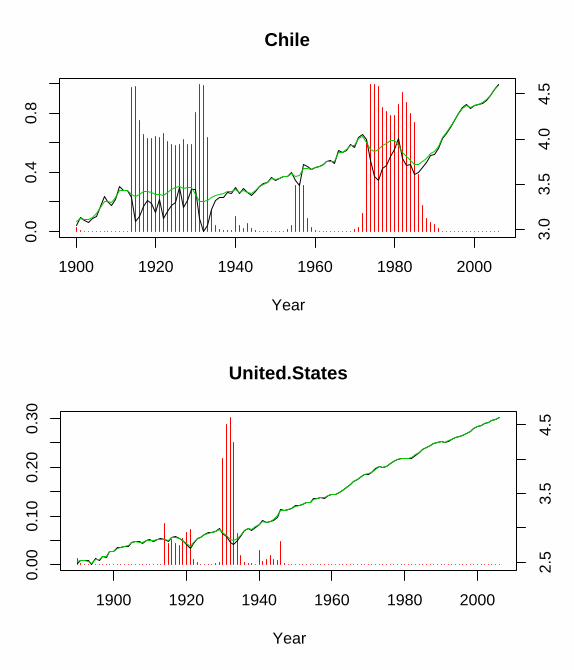
1900 1920 1940 1960 1980 2000

0.00

0.10

0.20

0.30

United.States

Year

2.5

3.5

4.5

1900 1920 1940 1960 1980 2000

0.0

0.4

0.8

Chile

Year

3.0

3.5

4.0

4.5

0 5 10 15 20 25 30 35

−0.

50.

00.

51.

0

0 5 10 15 20 25

−0.

50.

00.

51.

0

0 5 10 15 20 25 30 35

−0.

50.

00.

51.

0

Equity Premium

Den

sity

0.00 0.05 0.10 0.15

05

1015

20

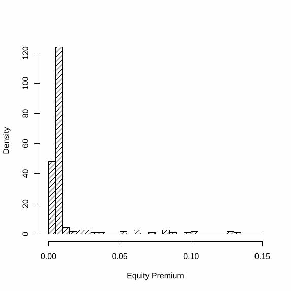
Equity Premium

Den

sity

0.00 0.05 0.10 0.15

020

4060

8010

012

0