Crime in Europe and the United States: dissecting the ‘reversal of misfortunes

SUMMARY

Contrary to common perceptions, today both property and violent crimes (with

the exception of homicides) are more widespread in Europe than in the United

States, while the opposite was true thirty years ago. We label this fact as the

‘reversal of misfortunes’. We investigate what accounts for the reversal by

studying the causal impact of demographic changes, incarceration, abortion,

unemployment and immigration on crime. For this we use time series data

(1970–2008) from seven European countries and the United States. We find

that the demographic structure of the population and the incarceration rate are

important determinants of crime. Our results suggest that a tougher incarceration

policy may be an effective way to contrast crime in Europe. Our analysis does

not provide information on how incarceration policy should be made tougher nor

does it provide an answer to the question whether such a policy would also be

efficient from a cost-benefit point of view. We leave this to future research.

— Paolo Buonanno, Francesco Drago, Roberto Galbiati and Giulio Zanella

Crime

Economic Policy July 2011 Printed in Great Britain� CEPR, CES, MSH, 2011.

Crime in Europe and the UnitedStates: dissecting the ‘reversalof misfortunes’

Paolo Buonanno, Francesco Drago, Roberto Galbiati andGiulio Zanella

University of Bergamo; University of Naples Parthenope and CSEF; CNRS-EconomiX andDepartment of Economics Sciences-Po; University of Bologna

1. INTRODUCTION

Despite the interest of policymakers in crime and the long tradition of economic

analysis of delinquent behaviour, there is a surprising lack of quantitative research

on the determinants of crime and on the effects of crime control policies outside

the United States, particularly in Europe. Much of what we know is based on anal-

yses of American data,1 and is summarized by Levitt (2004) and Levitt and Miles

(2007).2 The primary goal of this paper is to fill this gap: we employ data on crime

in Europe as well, and perform a cross-country empirical investigation of crime

trends during the last 40 years. Here and in what follows, by Europe we mean

Austria, France, Germany, Italy, the Netherlands, Spain and the United Kingdom.

The paper was prepared for the October 2010 Panel Meeting of Economic Policy in Rome. We wish to thank Horst Entorf,

Denis Fougere, Annie Kensey, David Paton, Giovanni Peri, and Ben Vollaard for sharing data, as well three anonymous ref-

erees, our discussants at the 52nd EP Panel Meeting (Jerome Adda and Bas Jacobs), the Panel Meeting participants, and

Roger Bowles, Philip Cook, Francesco Fasani, Tommaso Frattini, Rene Levy, Olivier Marie, Inigo Ortiz, Aurelie Ouss,

Arnaud Philippe, Rodrigo Soares, Christian Traxler and Pablo Velasquez for useful suggestions.

The managing editor in charge of this paper was Jan van Ours.1 An exception is Cook and Khmilevska (2005), who compare crime rates across countries.2 Other important contributions in criminology and economics to the understanding of crime trends in the US include Blum-

stein and Wallman (2000), Cook and Laub (2002), and Zimring (2006).

CRIME 349

Economic Policy July 2011 pp. 347–385 Printed in Great Britain� CEPR, CES, MSH, 2011.

Although this choice is primarily driven by data availability, these seven countries

account for more than 80% of the pre-2004 population of the current European

Union, with an aggregate population above 300 million – a figure comparable to

the US population.

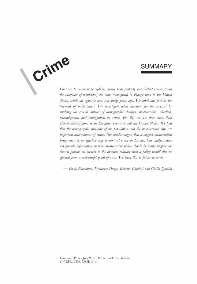
It is well known that the United States experienced an unexpected drop in

crime rates after 1990. In Europe, on the contrary, crime rates have been on the

rise since at least 1970. Contrary to common perceptions, crime is today more

widespread in Europe than in the United States, while the opposite was true 30

years ago. This fact, which we label the ‘reversal of misfortunes’, is documented in

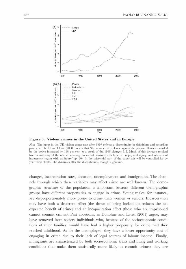
Figures 1–3. Figure 1 shows the dynamics of the total crime rate (crimes of any

kind reported to the police per 1,000 inhabitants) in the United States and in

Europe. In 1970 the aggregate crime rate in the seven European countries we con-

sider was 63% of the corresponding US figure, but by 2007 it was 85% higher

than in the United States. This striking reversal results from a steady increase in

the total crime rate in Europe during the last 40 years, and the decline in the US

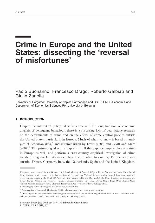
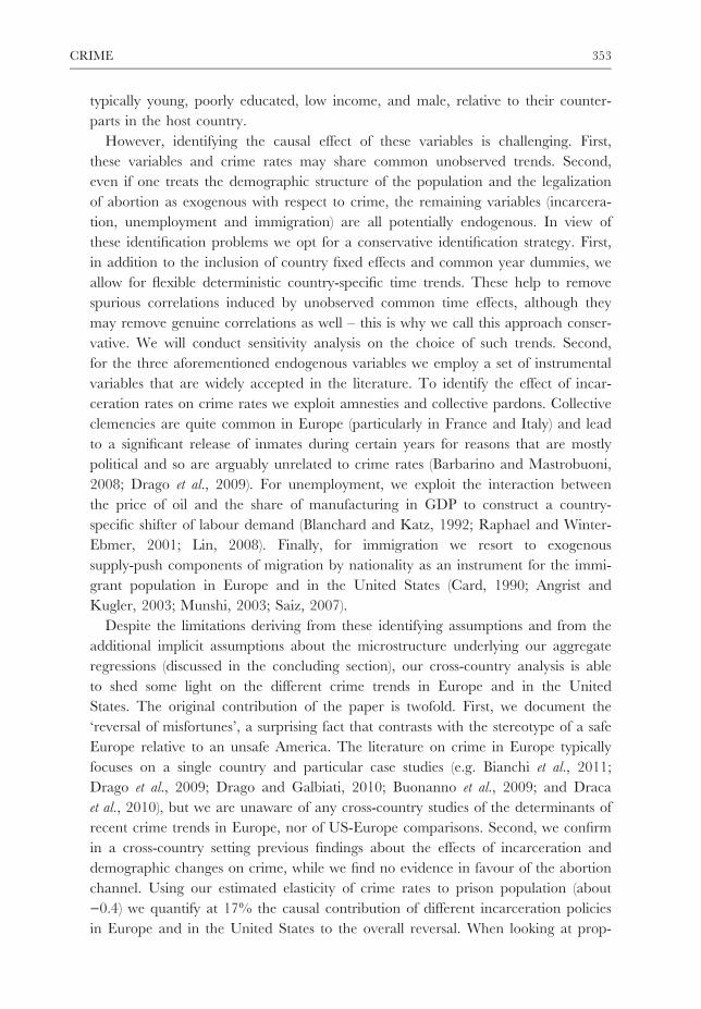
rate after 1990. The reversal of misfortunes is also observed for property and

violent crimes. Figure 2 documents the trends in the property crime rate. Although

in this case Europe and the United States have been moving along a common

(a)

(b)

Figure 1. Total crime in the United States and in Europe

350 PAOLO BUONANNO ET AL.

trend since the early 1990s, the European rate in 2007 was still 20% above the

US rate, while in 1970 the Europe/US ratio was below 30%. The same pattern is

found when looking at individual countries, with the exceptions of France and

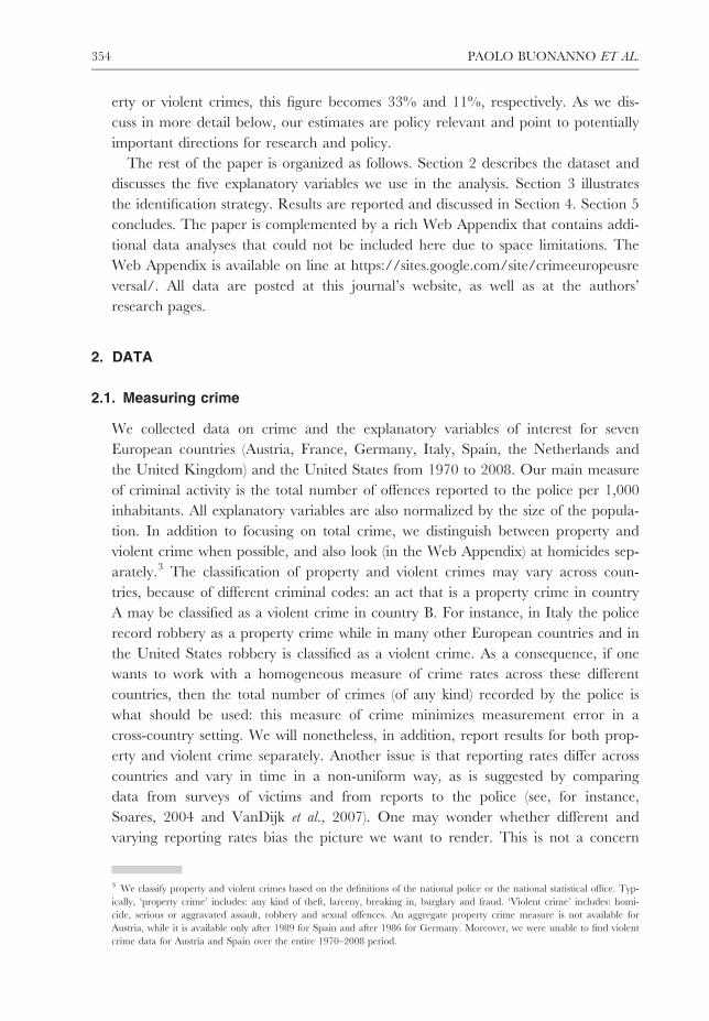
Italy. Figure 3 shows the reversal for violent crimes: in 1970 the violent crime rate

in Europe was 62% of the corresponding rate in the United States. By 2008 it was

more than twice the US figure. We discuss later how varying reporting rates may

alter these patterns.

These pictures reveal a substantial divergence between crime trends in Europe

and the United States. Apparently, the American experience is a story of success in

crime control when compared to what happened on the other side of the Atlantic.

This makes a cross-country investigation of the determinants of crime rates an

interesting research question: although the United States and Europe have different

social and economic structures, it is natural to ask whether the different dynamics

of the crime rates in the two areas can be explained by the different dynamics of

the factors emphasized by the economics of crime.

We address this question by using a subset of such explanatory variables, for

which we have been able to collect long-term cross-country series: demographic

(b)

(a)

Figure 2. Property crimes in the United States and in Europe

CRIME 351

changes, incarceration rates, abortion, unemployment and immigration. The chan-

nels through which these variables may affect crime are well known. The demo-

graphic structure of the population is important because different demographic

groups have different propensities to engage in crime. Young males, for instance,

are disproportionately more prone to crime than women or seniors. Incarceration

may have both a deterrent effect (the threat of being locked up reduces the net

expected benefit of crime) and an incapacitation effect (those who are imprisoned

cannot commit crimes). Past abortions, as Donohue and Levitt (2001) argue, may

have removed from society individuals who, because of the socioeconomic condi-

tions of their families, would have had a higher propensity for crime had they

reached adulthood. As for the unemployed, they have a lower opportunity cost of

engaging in crime due to their lack of legal sources of labour income. Finally,

immigrants are characterized by both socioeconomic traits and living and working

conditions that make them statistically more likely to commit crimes: they are

(a)

(b)

Figure 3. Violent crimes in the United States and in Europe

Note: The jump in the UK violent crime rate after 1997 reflects a discontinuity in definitions and recordingpractices. The Home Office (2008) notices that ‘the number of violence against the person offences recordedby the police increased by 118 per cent as a result of the 1998 changes [...]. Much of this increase resultedfrom a widening of the offence coverage to include assaults with little or no physical injury, and offences ofharassment (again with no injury)’ (p. 60). In the inferential part of the paper this will be controlled for byyear fixed effects. The dynamics after the discontinuity, though is genuine.


typically young, poorly educated, low income, and male, relative to their counter-

parts in the host country.

However, identifying the causal effect of these variables is challenging. First,

these variables and crime rates may share common unobserved trends. Second,

even if one treats the demographic structure of the population and the legalization

of abortion as exogenous with respect to crime, the remaining variables (incarcera-

tion, unemployment and immigration) are all potentially endogenous. In view of

these identification problems we opt for a conservative identification strategy. First,

in addition to the inclusion of country fixed effects and common year dummies, we

allow for flexible deterministic country-specific time trends. These help to remove

spurious correlations induced by unobserved common time effects, although they

may remove genuine correlations as well – this is why we call this approach conser-

vative. We will conduct sensitivity analysis on the choice of such trends. Second,

for the three aforementioned endogenous variables we employ a set of instrumental

variables that are widely accepted in the literature. To identify the effect of incar-

ceration rates on crime rates we exploit amnesties and collective pardons. Collective

clemencies are quite common in Europe (particularly in France and Italy) and lead

to a significant release of inmates during certain years for reasons that are mostly

political and so are arguably unrelated to crime rates (Barbarino and Mastrobuoni,

2008; Drago et al., 2009). For unemployment, we exploit the interaction between

the price of oil and the share of manufacturing in GDP to construct a country-

specific shifter of labour demand (Blanchard and Katz, 1992; Raphael and Winter-

Ebmer, 2001; Lin, 2008). Finally, for immigration we resort to exogenous

supply-push components of migration by nationality as an instrument for the immi-

grant population in Europe and in the United States (Card, 1990; Angrist and

Kugler, 2003; Munshi, 2003; Saiz, 2007).

Despite the limitations deriving from these identifying assumptions and from the

additional implicit assumptions about the microstructure underlying our aggregate

regressions (discussed in the concluding section), our cross-country analysis is able

to shed some light on the different crime trends in Europe and in the United

States. The original contribution of the paper is twofold. First, we document the

‘reversal of misfortunes’, a surprising fact that contrasts with the stereotype of a safe

Europe relative to an unsafe America. The literature on crime in Europe typically

focuses on a single country and particular case studies (e.g. Bianchi et al., 2011;

Drago et al., 2009; Drago and Galbiati, 2010; Buonanno et al., 2009; and Draca

et al., 2010), but we are unaware of any cross-country studies of the determinants of

recent crime trends in Europe, nor of US-Europe comparisons. Second, we confirm

in a cross-country setting previous findings about the effects of incarceration and

demographic changes on crime, while we find no evidence in favour of the abortion

channel. Using our estimated elasticity of crime rates to prison population (about

)0.4) we quantify at 17% the causal contribution of different incarceration policies

in Europe and in the United States to the overall reversal. When looking at prop-

CRIME 353

erty or violent crimes, this figure becomes 33% and 11%, respectively. As we dis-

cuss in more detail below, our estimates are policy relevant and point to potentially

important directions for research and policy.

The rest of the paper is organized as follows. Section 2 describes the dataset and

discusses the five explanatory variables we use in the analysis. Section 3 illustrates

the identification strategy. Results are reported and discussed in Section 4. Section 5

concludes. The paper is complemented by a rich Web Appendix that contains addi-

tional data analyses that could not be included here due to space limitations. The

Web Appendix is available on line at https://sites.google.com/site/crimeeuropeusre

versal/. All data are posted at this journal’s website, as well as at the authors’

research pages.

2. DATA

2.1. Measuring crime

We collected data on crime and the explanatory variables of interest for seven

European countries (Austria, France, Germany, Italy, Spain, the Netherlands and

the United Kingdom) and the United States from 1970 to 2008. Our main measure

of criminal activity is the total number of offences reported to the police per 1,000

inhabitants. All explanatory variables are also normalized by the size of the popula-

tion. In addition to focusing on total crime, we distinguish between property and

violent crime when possible, and also look (in the Web Appendix) at homicides sep-

arately.3 The classification of property and violent crimes may vary across coun-

tries, because of different criminal codes: an act that is a property crime in country

A may be classified as a violent crime in country B. For instance, in Italy the police

record robbery as a property crime while in many other European countries and in

the United States robbery is classified as a violent crime. As a consequence, if one

wants to work with a homogeneous measure of crime rates across these different

countries, then the total number of crimes (of any kind) recorded by the police is

what should be used: this measure of crime minimizes measurement error in a

cross-country setting. We will nonetheless, in addition, report results for both prop-

erty and violent crime separately. Another issue is that reporting rates differ across

countries and vary in time in a non-uniform way, as is suggested by comparing

data from surveys of victims and from reports to the police (see, for instance,

Soares, 2004 and VanDijk et al., 2007). One may wonder whether different and

varying reporting rates bias the picture we want to render. This is not a concern

3 We classify property and violent crimes based on the definitions of the national police or the national statistical office. Typ-

ically, ‘property crime’ includes: any kind of theft, larceny, breaking in, burglary and fraud. ‘Violent crime’ includes: homi-

cide, serious or aggravated assault, robbery and sexual offences. An aggregate property crime measure is not available for

Austria, while it is available only after 1989 for Spain and after 1986 for Germany. Moreover, we were unable to find violent

crime data for Austria and Spain over the entire 1970–2008 period.


when doing inference (employing country fixed effects, year fixed effects, and coun-

try-specific trends absorbs the resulting variation), but a bias could be present when

looking at plain sample statistics.

The Web Appendix expands on these measurement issues. First, we take a sepa-

rate look at voluntary homicides, which have the same definition everywhere and

whose reporting rate is virtually 100% (very few voluntary homicides are not known

to the police or misclassified as, for instance, suicides). Second, we correct crime

rates using reporting rates from victimization surveys when possible. In both cases

we produce evidence consistent with the reversal of misfortunes: this does not seem

an artefact of measurement errors.

2.2. Crime in Europe and in the United States: stylized facts

Figures 1–3 reveal four important facts:

• Crime rates in Europe tend to move in parallel;

• Crime rates in Europe increased sharply from 1970 to 1990; the total crime rate

stabilized afterwards, with property crimes decreasing since the early 2000s and

violent crimes increasing steadily (with a few exceptions);

• Crime rates in the United States increased from 1970 to 1980, have no obvious

trend in the 1980s and decline sharply in the 1990s. The rate of decline is less

sharp from 2000 onward;

• Crime rates in the United States were above the corresponding rates in Europe

in 1970, but they have been below European levels in recent years (with a few

exceptions for property crime).

The decline in the US crime rates that began in the 1990s is discussed extensively

in the literature. Given the trend in the 1970s and 1980s, this decline was a sur-

prise and puzzled many analysts. According to Levitt (2004), increased incarcera-

tion, more police, the decline of crack and the legalization of abortion played an

important role in this process. Imrohoroglu et al. (2004) offer additional explana-

tions for the decline in property crimes: a higher probability of apprehension, the

stronger economy, and a change in the demographic structure – most notably a

decline in the demographic weight of young men. The further decline during the

last ten years is consistent with these findings. First, the number of police officers in

the United States has grown further since the early 2000s. Second, in the United

States a substantial fraction of the criminally active population at the end of the

1990s was born prior to the legalization of abortion. The fact that cohorts born

after the legalization of abortion reach adulthood is consistent with the decreasing

trend if the Donohue and Levitt (2001) explanation is correct. Third, the demo-

graphic weight of young Americans has further declined. Fourth, consistently with

the slowdown in the US crime trend during the 2000s, crack-related crimes and

prison population apparently reached a steady state after the end of the 1990s.

CRIME 355

2.3. Five factors that may explain crime trends

As discussed in Section 1, the economics of crime suggests taking into account at

least two groups of variables that can explain crime rates. The first group includes

factors that directly influence the possibility of committing a crime and its opportu-

nity cost: police numbers, incarceration and unemployment. In particular, police

numbers and the prison population affect deterrence and incapacitation, and are

under the direct control of policymakers. Unfortunately, we are unable to include

police numbers in our analysis for two reasons. First, there is a lack of reliable

annual data on police forces in Europe before the mid-1990s. Second, we lack a

credible instrumental variable for which adequate data can be put together. The

second group includes sociodemographic variables, namely the age structure of

the population, and the abortion and immigration rates. The explanatory vari-

ables we use are the following: the share of males aged 15–34, the stock of

immigrants relative to the population, the abortion rate (defined as the propor-

tion of unborn children who would have been at least 18 years old in a given

year over the total population), the unemployment rate and the incarceration

rate. In the remainder of this section we discuss in detail what is known about

the relation between these variables and crime, and we document their dynamics

in our sample.

2.3.1. Demographics. It is well known in criminology that young males are statisti-

cally more likely to be offenders than any other demographic group. Levitt and

Lochner (2001) note that 18-year-old individuals are five times more likely to be

arrested for a property crime in the United States than their 35-year-old counter-

parts. For violent crime this ratio is 2:1. The same authors document that in 1997

those between 15 and 19 years old constituted 7% of the population but accounted

for over 20% of arrests for violent offences. In the light of these facts, the profound

demographic change caused in the United States by the ageing of the baby boom-

ers has been considered a potentially important driver in the decline in crime rates

in the United States during the 1990s. Levitt (2004) notes that people over 65 have

per-capita arrest rates approximately 2% the level of 15- to 19-year-olds, but claims

that the change in the age structure of the population played little role in explain-

ing the drop in crime. Imrohoroglu et al. (2004) observe that the share of the popu-

lation between 15 and 25 years old declined from 20.5% to 15.1% in the same

period, and claim that this accounts for 11% of the total drop in property crime

(the rate per 100 inhabitants in the United States dropped from 5.60 in 1980 to

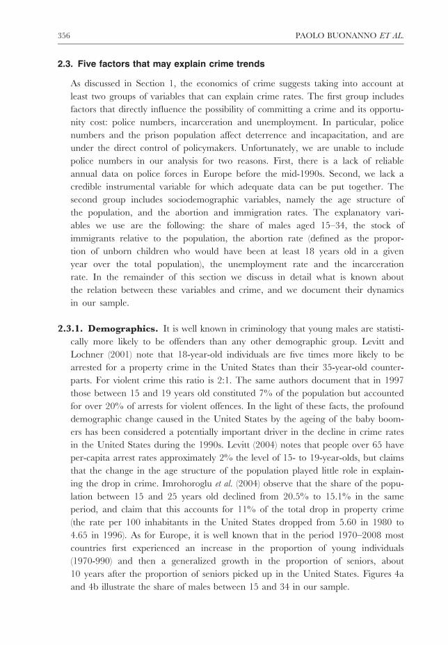
4.65 in 1996). As for Europe, it is well known that in the period 1970–2008 most

countries first experienced an increase in the proportion of young individuals

(1970-990) and then a generalized growth in the proportion of seniors, about

10 years after the proportion of seniors picked up in the United States. Figures 4a

and 4b illustrate the share of males between 15 and 34 in our sample.


2.3.2. Immigration. There are several reasons why immigrants and natives may

have different propensities to engage in crime. Part of this difference reflects the

migration process. Immigrants from less developed to more developed countries are

typically young, poorly educated and male. This makes them statistically more

likely to engage in crime. Thus, if we draw random samples of immigrants and

natives in a given country after conditioning on certain socioeconomic characteris-

tics, the two groups would probably have very similar criminal attitudes. In this

sense immigration may mechanically affect delinquency rates in receiving countries.

Furthermore, natives and immigrants may have a different opportunity cost of

crime. For instance, they may face different labour market prospects of working

legally, and they may face different probabilities of being convicted and different

costs of conviction, for instance because of the possibility of being deported.

Few empirical papers have investigated the relationship between immigration

and crime. Using individual data, Butcher and Piehl (1998b, 2005) find that current

immigrants in the United States have lower incarceration rates than natives, while

the pattern is reversed for the early 1900s (Moehling and Piehl, 2007). Using aggre-

gate data from US metropolitan areas in the 1980s, Butcher and Piehl (1998a)

conclude that the inflow of immigrants had no significant impact on crime rates.

Finally, Borjas et al. (2010) argue that recent immigrants have contributed to the

(a)

(b)

Figure 4. Share of young males (15–34) in the United States and in Europe

CRIME 357

criminal activity of native black males by displacing them from the labour market.

Evidence for European countries is even scarcer. Bianchi et al. (2011) examine the

empirical relationship between immigration and crime across Italian provinces dur-

ing the period 1990–2003. Drawing on police administrative records, they first

document that the size of the immigrant population is positively correlated with the

incidence of property crimes and with the overall crime rate. Then, using instru-

mental variables based on immigration toward destination countries other than

Italy, they find no evidence of a causal effect of immigration on crime in Italy.

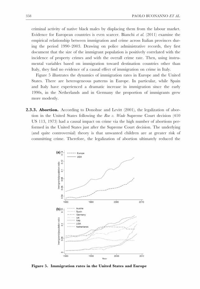
Figure 5 illustrates the dynamics of immigration rates in Europe and the United

States. There are heterogeneous patterns in Europe. In particular, while Spain

and Italy have experienced a dramatic increase in immigration since the early

1990s, in the Netherlands and in Germany the proportion of immigrants grew

more modestly.

2.3.3. Abortion. According to Donohue and Levitt (2001), the legalization of abor-

tion in the United States following the Roe v. Wade Supreme Court decision (410

US 113, 1973) had a causal impact on crime via the high number of abortions per-

formed in the United States just after the Supreme Court decision. The underlying

(and quite controversial) theory is that unwanted children are at greater risk of

committing crime. Therefore, the legalization of abortion ultimately reduced the

(a)

(b)

Figure 5. Immigration rates in the United States and Europe


birth of children who, had they been born, would have been at greater risk of com-

mitting crimes when they reached their teenage years. Levitt (2004) refers to various

studies supporting this hypothesis and showing that children born because their

mothers were denied abortion were substantially more likely to be involved in

crime, even when controlling for the income, age, education and health of the

mother. Further recent evidence supports this idea by showing that the legalization

of abortion reduced out-of-wedlock teen childbearing (Donohue et al., 2009). A

lively debate followed the article by Donohue and Levitt (2001),4 but the key find-

ings of the original article have so far proved robust. A discussion of the abortion

hypothesis is beyond the scope of this paper but the extension of the analysis to our

panel of European countries is important to provide further evidence along this line

of research.

In Europe the legalization of abortion did not follow a uniform pattern. Some

countries in our dataset legalized abortion in the 1970s, as did the United States,

others later.5 To date, to the best of our knowledge, the only papers studying the

relationship between abortion and crime in European countries are Pop-Eleches

(2006) and Kahane et al. (2007), who focus on Romania and on England and

Wales, respectively. The evidence from these studies is mixed. Pop-Eleches (2006)

exploits abortion bans during the Ceausescu era in Romania as a source of identifi-

cation and finds results in line with Donohue and Levitt (2001), while Kahane et al.

(2007) employ panel data and show that Donohue and Levitt’s result does not hold

in England and Wales when one uses a different abortion index.

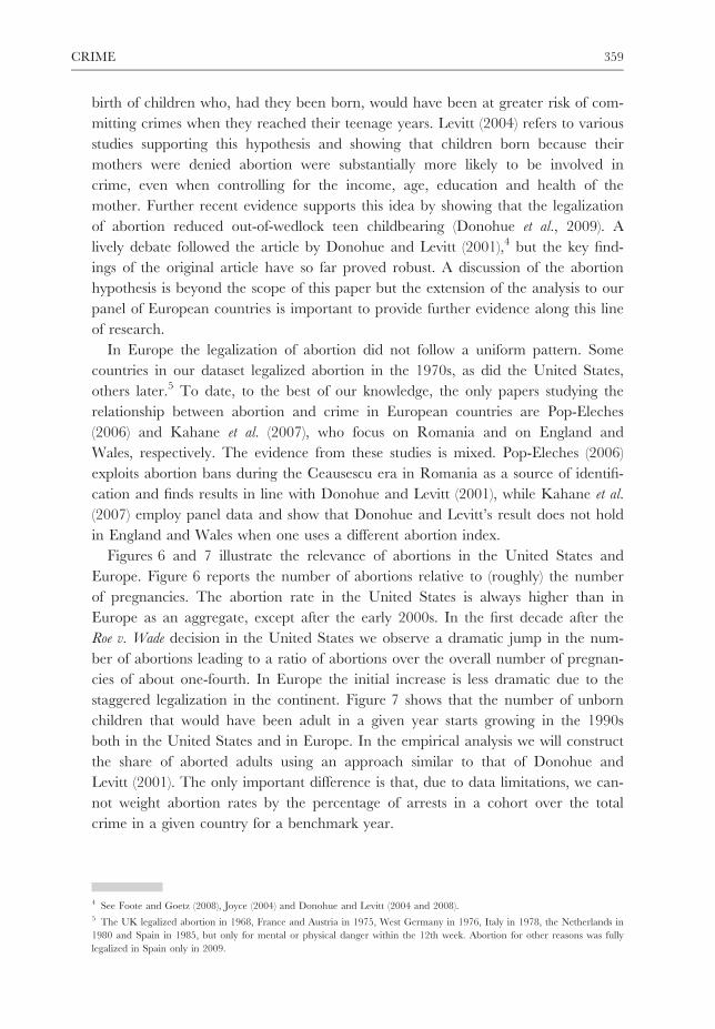
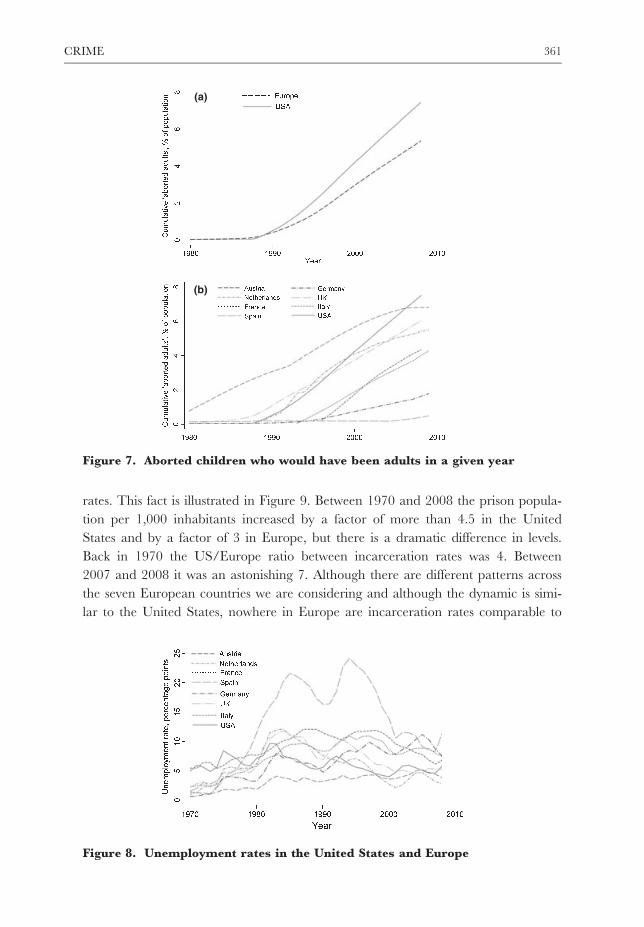
Figures 6 and 7 illustrate the relevance of abortions in the United States and

Europe. Figure 6 reports the number of abortions relative to (roughly) the number

of pregnancies. The abortion rate in the United States is always higher than in

Europe as an aggregate, except after the early 2000s. In the first decade after the

Roe v. Wade decision in the United States we observe a dramatic jump in the num-

ber of abortions leading to a ratio of abortions over the overall number of pregnan-

cies of about one-fourth. In Europe the initial increase is less dramatic due to the

staggered legalization in the continent. Figure 7 shows that the number of unborn

children that would have been adult in a given year starts growing in the 1990s

both in the United States and in Europe. In the empirical analysis we will construct

the share of aborted adults using an approach similar to that of Donohue and

Levitt (2001). The only important difference is that, due to data limitations, we can-

not weight abortion rates by the percentage of arrests in a cohort over the total

crime in a given country for a benchmark year.

4 See Foote and Goetz (2008), Joyce (2004) and Donohue and Levitt (2004 and 2008).5 The UK legalized abortion in 1968, France and Austria in 1975, West Germany in 1976, Italy in 1978, the Netherlands in

1980 and Spain in 1985, but only for mental or physical danger within the 12th week. Abortion for other reasons was fully

legalized in Spain only in 2009.

CRIME 359

2.3.4. Unemployment. According to the benchmark economic model of crime

(Becker, 1968; Ehrlich, 1973), labour market opportunities may affect a rational

individual’s decision to engage in crime: if legal income opportunities are less lucra-

tive than the expected gains from crime, individuals will opt for the latter. There-

fore, unemployment may lead to an increase in crime through two channels. First,

the expected returns from legal work decrease if the probability of being unem-

ployed is higher. Second, given a downward sloping labour demand curve, more

unemployment is associated with a lower wage rate. These two effects contribute to

reducing the opportunity cost of crime. Hence, we can expect unemployment to

have a positive effect on the crime rate. Recent empirical studies employing panel

data at the state or regional level (Raphael and Winter-Ebmer, 2001; Gould et al.,

2002; Lin, 2008; Oster and Agell, 2007; Fougere et al., 2009) reach a consensus that

increasing unemployment contributes to an increase in property crimes (although

the magnitude is not large) and does not significantly affect violent crimes. Imro-

horoglu et al. (2004), on the contrary, conclude that the effect of unemployment on

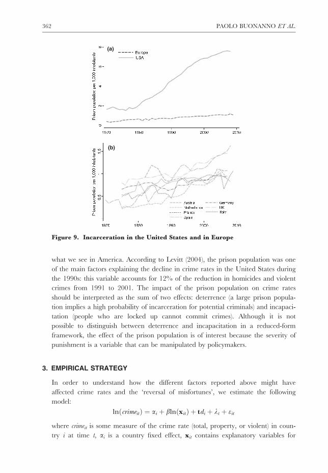
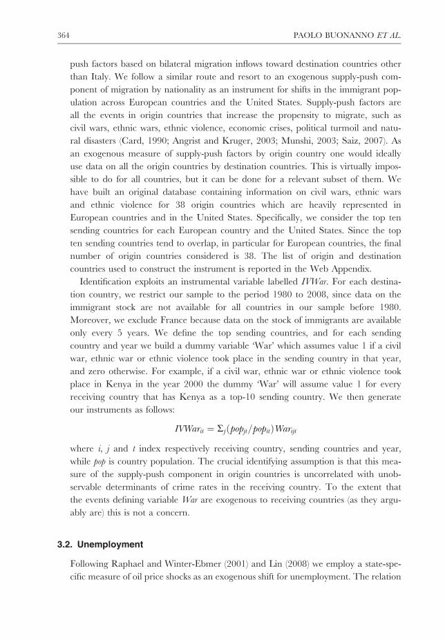
crime is negligible. Figure 8 reports the dynamics of the unemployment rates for

the eight countries under investigation.

2.3.5. Incarceration. Of all the explanatory variables we are considering, the most

striking difference between Europe and the United States pertains to incarceration

(a)

(b)

Figure 6. Abortion rates in the United States and Europe


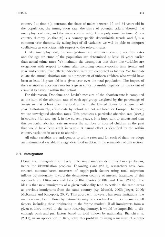
rates. This fact is illustrated in Figure 9. Between 1970 and 2008 the prison popula-

tion per 1,000 inhabitants increased by a factor of more than 4.5 in the United

States and by a factor of 3 in Europe, but there is a dramatic difference in levels.

Back in 1970 the US/Europe ratio between incarceration rates was 4. Between

2007 and 2008 it was an astonishing 7. Although there are different patterns across

the seven European countries we are considering and although the dynamic is simi-

lar to the United States, nowhere in Europe are incarceration rates comparable to

(b)

(a)

Figure 7. Aborted children who would have been adults in a given year

Figure 8. Unemployment rates in the United States and Europe

CRIME 361

what we see in America. According to Levitt (2004), the prison population was one

of the main factors explaining the decline in crime rates in the United States during

the 1990s: this variable accounts for 12% of the reduction in homicides and violent

crimes from 1991 to 2001. The impact of the prison population on crime rates

should be interpreted as the sum of two effects: deterrence (a large prison popula-

tion implies a high probability of incarceration for potential criminals) and incapaci-

tation (people who are locked up cannot commit crimes). Although it is not

possible to distinguish between deterrence and incapacitation in a reduced-form

framework, the effect of the prison population is of interest because the severity of

punishment is a variable that can be manipulated by policymakers.

3. EMPIRICAL STRATEGY

In order to understand how the different factors reported above might have

affected crime rates and the ‘reversal of misfortunes’, we estimate the following

model:

lnðcrimeitÞ ¼ ai þ blnðxitÞ þ tdi þ kt þ eit

where crimeit is some measure of the crime rate (total, property, or violent) in coun-

try i at time t, ai is a country fixed effect, xit contains explanatory variables for

(a)

(b)

Figure 9. Incarceration in the United States and in Europe


country i at time t (a constant, the share of males between 15 and 34 years old in

the population, the immigration rate, the share of potential adults aborted, the

unemployment rate, and the incarceration rate), t is a polynomial in time, di is a

country dummy (so that tdi is a country-specific deterministic trend), and kt is a

common year dummy. By taking logs of all variables we will be able to interpret

coefficients as elasticities with respect to the relevant rates.

Unlike unemployment, the immigration rate and incarceration, abortion rates

and the age structure of the population are determined at least 15 years earlier

than actual crime rates. We maintain the assumption that these two variables are

exogenous with respect to crime after including country-specific time trends and

year and country fixed effects. Abortion rates are computed as follows. We first cal-

culate the annual abortion rate as a proportion of unborn children who would have

been at least 18 years old in a given year over the total population. The impact of

the variation in abortion rates for a given cohort plausibly depends on the extent of

criminal behaviour within that cohort.

For this reason, Donohue and Levitt’s measure of the abortion rate is computed

as the sum of the abortion rate of each age group weighted by the percentage of

arrests in that cohort over the total crime in the United States for a benchmark

year. Unfortunately, crime data by cohort are not available for Europe. Therefore,

we use unweighted abortion rates. This produces a particular abortion rate (abortikt)

in country i for any age k, in the current year, t. It is important to understand that

this particular abortion rate measures the number of aborted children in the past

that would have been adult in year t. A causal effect is identified by the within

country variation in access to abortion.

All other variables are endogenous to crime rates and for each of them we adopt

an instrumental variable strategy, described in detail in the remainder of this section.

3.1. Immigration

Crime and immigration are likely to be simultaneously determined in equilibrium,

hence the identification problem. Following Card (2001), researchers have con-

structed outcome-based measures of supply-push factors using total migration

inflows by nationality toward the destination country of interest. Examples of this

approach are Ottaviano and Peri (2006), Cortes (2008), and Card (2009). The

idea is that new immigrants of a given nationality tend to settle in the same areas

as previous immigrants from the same country (e.g. Munshi, 2003; Jaeger, 2006;

McKenzie and Rapoport, 2007). This approach, however, has some limitations. To

mention one, total inflows by nationality may be correlated with local demand-pull

factors, including those originating in the ‘crime market’. If all immigrants from a

given country moved to the same receiving country, it would be impossible to dis-

entangle push and pull factors based on total inflows by nationality. Bianchi et al.

(2011), in an application to Italy, solve this problem by using a measure of supply-

CRIME 363

push factors based on bilateral migration inflows toward destination countries other

than Italy. We follow a similar route and resort to an exogenous supply-push com-

ponent of migration by nationality as an instrument for shifts in the immigrant pop-

ulation across European countries and the United States. Supply-push factors are

all the events in origin countries that increase the propensity to migrate, such as

civil wars, ethnic wars, ethnic violence, economic crises, political turmoil and natu-

ral disasters (Card, 1990; Angrist and Kruger, 2003; Munshi, 2003; Saiz, 2007). As

an exogenous measure of supply-push factors by origin country one would ideally

use data on all the origin countries by destination countries. This is virtually impos-

sible to do for all countries, but it can be done for a relevant subset of them. We

have built an original database containing information on civil wars, ethnic wars

and ethnic violence for 38 origin countries which are heavily represented in

European countries and in the United States. Specifically, we consider the top ten

sending countries for each European country and the United States. Since the top

ten sending countries tend to overlap, in particular for European countries, the final

number of origin countries considered is 38. The list of origin and destination

countries used to construct the instrument is reported in the Web Appendix.

Identification exploits an instrumental variable labelled IVWar. For each destina-

tion country, we restrict our sample to the period 1980 to 2008, since data on the

immigrant stock are not available for all countries in our sample before 1980.

Moreover, we exclude France because data on the stock of immigrants are available

only every 5 years. We define the top sending countries, and for each sending

country and year we build a dummy variable ‘War’ which assumes value 1 if a civil

war, ethnic war or ethnic violence took place in the sending country in that year,

and zero otherwise. For example, if a civil war, ethnic war or ethnic violence took

place in Kenya in the year 2000 the dummy ‘War’ will assume value 1 for every

receiving country that has Kenya as a top-10 sending country. We then generate

our instruments as follows:

IVWarit ¼ Rjðpopjt=popitÞWarijt

where i, j and t index respectively receiving country, sending countries and year,

while pop is country population. The crucial identifying assumption is that this mea-

sure of the supply-push component in origin countries is uncorrelated with unob-

servable determinants of crime rates in the receiving country. To the extent that

the events defining variable War are exogenous to receiving countries (as they argu-

ably are) this is not a concern.

3.2. Unemployment

Following Raphael and Winter-Ebmer (2001) and Lin (2008) we employ a state-spe-

cific measure of oil price shocks as an exogenous shift for unemployment. The relation


between the unemployment rate and the price of oil has been discussed and analysed

by Blanchard and Katz (1992), among others. This approach allows us to isolate the

exogenous (with respect to crime) component of variations in unemployment in the

data and so to identify a causal effect of unemployment on crime. The instrument is

constructed as follows. For each country and each year, we define the proportion of

employment in the manufacturing sector. This allows us to roughly measure the rele-

vance of energy-intensive industries. Next, by using the world price of crude oil (spot

price, West Texas Intermediate), we construct a measure of state-specific exposure to

oil shocks by interacting the proportion of employment in manufacturing and the

price of oil. The idea behind this instrument is simple. Since there are no short-run

substitutes for energy in manufacturing and since the price of oil is presumably unaf-

fected by the economic activity of the eight countries in our panel, any variation in

the price of oil generates an exogenous variation in unemployment – manufacturers

must reduce their consumption of energy by reducing output and employment. The

identifying assumption is that such shocks do not affect crime directly.

3.3. Incarceration

The incarceration rate is endogenous because it may simply reflect the extent of

crime: the more people engage in crime the larger the prison population. Ideally,

one would like to exploit quasi-experiments that exogenously alter the imprison-

ment rate. This is what Levitt (1996), Drago et al. (2009) and Barbarino and

Mastrobuoni (2008) do for the United States and Italy, respectively. Levitt uses

prison overcrowding litigation: court decisions in the United States may limit the

growth rates of inmates in state prisons for reasons that have nothing to do with

the incidence of crime. This generates an exogenous source of variation in the

prison population relative to control states. Drago et al. (2009) use a collective par-

don implemented in Italy in 2006 to reduce the population in overcrowded prisons

to identify the deterrent effect of an increase in expected prison sentences.6 Barbari-

no and Mastrobuoni (2008) exploit a series of prison amnesties in Italy to estimate

the incapacitation effect of prison. These studies have the advantage of exploiting

credible sources of exogenous variation in the prison population or expected prison

sentences. However, they refer to single countries.

We follow this line of research and exploit amnesties across different countries

to construct an instrument for prison population. Specifically, we first consider

prison population lagged by one year – the number of inmates in prison statistics

refers to the stock at the end of a given year. Therefore, our aim is to identify the

effect of the prison population at time t–1 on crime rates at time t. The prison

6 The collective pardon bill commuted actual sentences into expected sentences for those with less than three years of resid-

ual sentence. Thus, by exploiting the plausible exogeneity of residual sentences, Drago et al. (2009) can provide an estimate of

the deterrent effect of prison sentences.

CRIME 365

population at time t–1 in a given country is instrumented with a dummy that is

equal to one if in the same year (t–1) an amnesty was passed in that country. The

identifying assumption is that an amnesty affects crime rates only via the induced

variation in prison population. We believe this assumption is credible. Many of the

collective pardons and amnesties implemented by European countries between

1970 and 2008 were officially motivated by either political or humanitarian rea-

sons. In many cases this is unquestionably so, as with the three consecutive amnes-

ties approved in Spain after the end of the Franco dictatorship. However, one

might suspect that in some cases such official motivations mask attempts to quickly

reduce prison overcrowding. If this were the case, then amnesties would be pre-

dictable by looking at the past evolution of crime rates. Below we present evidence

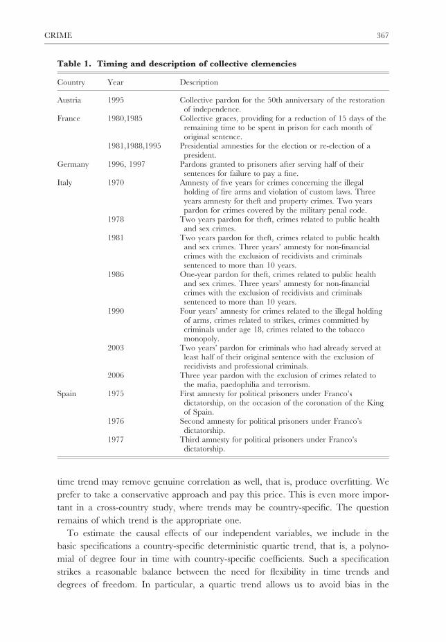
that this is not the case. We first report in Table 1 the timing and description of

the amnesties used in our dataset. The official motivations seem to be unrelated to

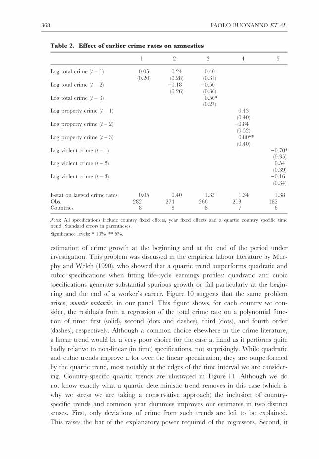
crime rates. As supporting evidence of this exclusion restriction, we report in

Table 2 the results a regression of amnesties at time t on crime rates in earlier

years. A significant relationship between past crime rates and amnesties would cast

doubts on the validity of the identification strategy: it would suggest that amnesties

are determined by or correlated to past trends in criminal activity. Table 2, how-

ever, shows that crime rates in earlier years do not systematically predict amnes-

ties. This is also true when we include crime rates with three lags. Given that in

some countries amnesties have occasionally been passed every other year, it is reas-

suring that crime rates one year, and two and three years earlier together do not

predict amnesties.

As in all instrumental variable estimates, the elasticity of crime rates to prison

population should be interpreted as a local average treatment effect (LATE). This

raises the question of whether our results can be generalized to countries (such as

the Netherlands, the United Kingdom and the United States) where no amnesty

was passed during the 40 years on which we focus. An additional issue is that the

only logically possible effect of amnesties is a reduction in the prison population,

while the interpretation of the elasticity we estimate is two-sided (it includes a deter-

rence and an incapacitation effect). While these problems arise commonly when

employing instrumental variables, it is important to keep them in mind when

attempting out-of-sample policy exercises.

3.4. Country specific time trends

It is common in longitudinal analyses to include a time trend to account for the

possible exogenous dynamics of the dependent variable of interest. Without doing

so, such dynamics could be wrongly interpreted as caused by some explanatory var-

iable that moves along a trend correlated (because of other underlying forces) with

the trend of the dependent variable. In other words, a time trend removes possible

spurious correlations. This comes at a price, though: superimposing an exogenous


time trend may remove genuine correlation as well, that is, produce overfitting. We

prefer to take a conservative approach and pay this price. This is even more impor-

tant in a cross-country study, where trends may be country-specific. The question

remains of which trend is the appropriate one.

To estimate the causal effects of our independent variables, we include in the

basic specifications a country-specific deterministic quartic trend, that is, a polyno-

mial of degree four in time with country-specific coefficients. Such a specification

strikes a reasonable balance between the need for flexibility in time trends and

degrees of freedom. In particular, a quartic trend allows us to avoid bias in the

Table 1. Timing and description of collective clemencies

Country Year Description

Austria 1995 Collective pardon for the 50th anniversary of the restorationof independence.

France 1980,1985 Collective graces, providing for a reduction of 15 days of theremaining time to be spent in prison for each month oforiginal sentence.

1981,1988,1995 Presidential amnesties for the election or re-election of apresident.

Germany 1996, 1997 Pardons granted to prisoners after serving half of theirsentences for failure to pay a fine.

Italy 1970 Amnesty of five years for crimes concerning the illegalholding of fire arms and violation of custom laws. Threeyears amnesty for theft and property crimes. Two yearspardon for crimes covered by the military penal code.

1978 Two years pardon for theft, crimes related to public healthand sex crimes.

1981 Two years pardon for theft, crimes related to public healthand sex crimes. Three years’ amnesty for non-financialcrimes with the exclusion of recidivists and criminalssentenced to more than 10 years.

1986 One-year pardon for theft, crimes related to public healthand sex crimes. Three years’ amnesty for non-financialcrimes with the exclusion of recidivists and criminalssentenced to more than 10 years.

1990 Four years’ amnesty for crimes related to the illegal holdingof arms, crimes related to strikes, crimes committed bycriminals under age 18, crimes related to the tobaccomonopoly.

2003 Two years’ pardon for criminals who had already served atleast half of their original sentence with the exclusion ofrecidivists and professional criminals.

2006 Three year pardon with the exclusion of crimes related tothe mafia, paedophilia and terrorism.

Spain 1975 First amnesty for political prisoners under Franco’sdictatorship, on the occasion of the coronation of the Kingof Spain.

1976 Second amnesty for political prisoners under Franco’sdictatorship.

1977 Third amnesty for political prisoners under Franco’sdictatorship.

CRIME 367

estimation of crime growth at the beginning and at the end of the period under

investigation. This problem was discussed in the empirical labour literature by Mur-

phy and Welch (1990), who showed that a quartic trend outperforms quadratic and

cubic specifications when fitting life-cycle earnings profiles: quadratic and cubic

specifications generate substantial spurious growth or fall particularly at the begin-

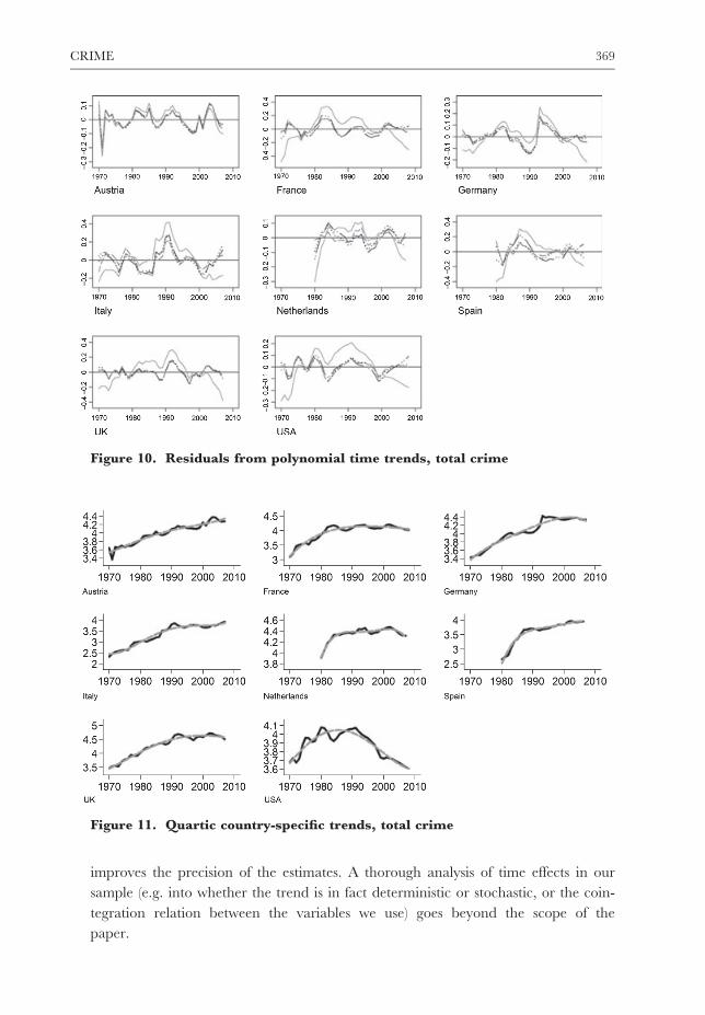
ning and the end of a worker’s career. Figure 10 suggests that the same problem

arises, mutatis mutandis, in our panel. This figure shows, for each country we con-

sider, the residuals from a regression of the total crime rate on a polynomial func-

tion of time: first (solid), second (dots and dashes), third (dots), and fourth order

(dashes), respectively. Although a common choice elsewhere in the crime literature,

a linear trend would be a very poor choice for the case at hand as it performs quite

badly relative to non-linear (in time) specifications, not surprisingly. While quadratic

and cubic trends improve a lot over the linear specification, they are outperformed

by the quartic trend, most notably at the edges of the time interval we are consider-

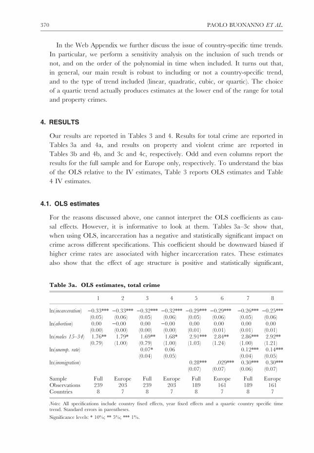
ing. Country-specific quartic trends are illustrated in Figure 11. Although we do

not know exactly what a quartic deterministic trend removes in this case (which is

why we stress we are taking a conservative approach) the inclusion of country-

specific trends and common year dummies improves our estimates in two distinct

senses. First, only deviations of crime from such trends are left to be explained.

This raises the bar of the explanatory power required of the regressors. Second, it

Table 2. Effect of earlier crime rates on amnesties

1 2 3 4 5

Log total crime (t – 1) 0.05 0.24 0.40(0.20) (0.28) (0.31)

Log total crime (t – 2) )0.18 )0.50(0.26) (0.36)

Log total crime (t – 3) 0.50*(0.27)

Log property crime (t – 1) 0.43(0.40)

Log property crime (t – 2) )0.84(0.52)

Log property crime (t – 3) 0.80**(0.40)

Log violent crime (t – 1) )0.70*(0.35)

Log violent crime (t – 2) 0.54(0.39)

Log violent crime (t – 3) )0.16(0.34)

F-stat on lagged crime rates 0.05 0.40 1.33 1.34 1.38Obs. 282 274 266 213 182Countries 8 8 8 7 6

Notes: All specifications include country fixed effects, year fixed effects and a quartic country specific timetrend. Standard errors in parentheses.

Significance levels: * 10%; ** 5%.


improves the precision of the estimates. A thorough analysis of time effects in our

sample (e.g. into whether the trend is in fact deterministic or stochastic, or the coin-

tegration relation between the variables we use) goes beyond the scope of the

paper.

Figure 10. Residuals from polynomial time trends, total crime

Figure 11. Quartic country-specific trends, total crime

CRIME 369

In the Web Appendix we further discuss the issue of country-specific time trends.

In particular, we perform a sensitivity analysis on the inclusion of such trends or

not, and on the order of the polynomial in time when included. It turns out that,

in general, our main result is robust to including or not a country-specific trend,

and to the type of trend included (linear, quadratic, cubic, or quartic). The choice

of a quartic trend actually produces estimates at the lower end of the range for total

and property crimes.

4. RESULTS

Our results are reported in Tables 3 and 4. Results for total crime are reported in

Tables 3a and 4a, and results on property and violent crime are reported in

Tables 3b and 4b, and 3c and 4c, respectively. Odd and even columns report the

results for the full sample and for Europe only, respectively. To understand the bias

of the OLS relative to the IV estimates, Table 3 reports OLS estimates and Table

4 IV estimates.

4.1. OLS estimates

For the reasons discussed above, one cannot interpret the OLS coefficients as cau-

sal effects. However, it is informative to look at them. Tables 3a–3c show that,

when using OLS, incarceration has a negative and statistically significant impact on

crime across different specifications. This coefficient should be downward biased if

higher crime rates are associated with higher incarceration rates. These estimates

also show that the effect of age structure is positive and statistically significant,

Table 3a. OLS estimates, total crime

1 2 3 4 5 6 7 8

ln(incarceration) )0.33*** )0.33*** )0.32*** )0.32*** )0.29*** )0.29*** )0.26*** )0.25***(0.05) (0.06) (0.05) (0.06) (0.05) (0.06) (0.05) (0.06)

ln(abortion) 0.00 )0.00 0.00 )0.00 0.00 0.00 0.00 0.00(0.00) (0.00) (0.00) (0.00) (0.01) (0.01) (0.01) (0.01)

ln(males 15–34) 1.76** 1.79* 1.69** 1.68* 2.91*** 2.84** 2.86*** 2.92**(0.79) (1.00) (0.79) (1.00) (1.03) (1.24) (1.00) (1.21)

ln(unemp. rate) 0.07* 0.06 0.12*** 0.14***(0.04) (0.05) (0.04) (0.05)

ln(immigration) 0.28*** .029*** 0.30*** 0.30***(0.07) (0.07) (0.06) (0.07)

Sample Full Europe Full Europe Full Europe Full EuropeObservations 239 203 239 203 189 161 189 161Countries 8 7 8 7 8 7 8 7


Significance levels: * 10%; ** 5%; *** 1%.


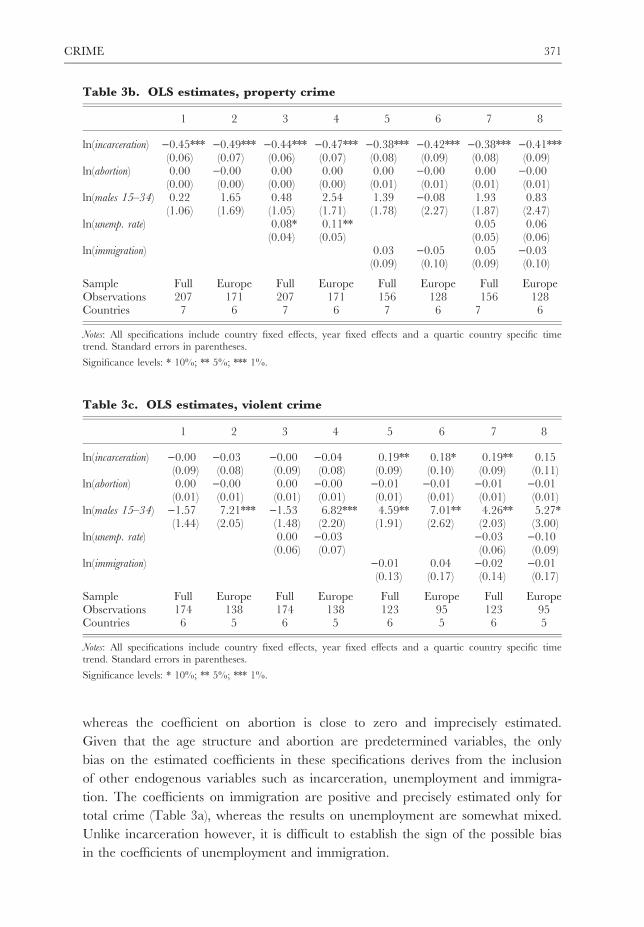
whereas the coefficient on abortion is close to zero and imprecisely estimated.

Given that the age structure and abortion are predetermined variables, the only

bias on the estimated coefficients in these specifications derives from the inclusion

of other endogenous variables such as incarceration, unemployment and immigra-

tion. The coefficients on immigration are positive and precisely estimated only for

total crime (Table 3a), whereas the results on unemployment are somewhat mixed.

Unlike incarceration however, it is difficult to establish the sign of the possible bias

in the coefficients of unemployment and immigration.

Table 3b. OLS estimates, property crime

1 2 3 4 5 6 7 8

ln(incarceration) )0.45*** )0.49*** )0.44*** )0.47*** )0.38*** )0.42*** )0.38*** )0.41***(0.06) (0.07) (0.06) (0.07) (0.08) (0.09) (0.08) (0.09)

ln(abortion) 0.00 )0.00 0.00 0.00 0.00 )0.00 0.00 )0.00(0.00) (0.00) (0.00) (0.00) (0.01) (0.01) (0.01) (0.01)

ln(males 15–34) 0.22 1.65 0.48 2.54 1.39 )0.08 1.93 0.83(1.06) (1.69) (1.05) (1.71) (1.78) (2.27) (1.87) (2.47)

ln(unemp. rate) 0.08* 0.11** 0.05 0.06(0.04) (0.05) (0.05) (0.06)

ln(immigration) 0.03 )0.05 0.05 )0.03(0.09) (0.10) (0.09) (0.10)




Table 3c. OLS estimates, violent crime

1 2 3 4 5 6 7 8

ln(incarceration) )0.00 )0.03 )0.00 )0.04 0.19** 0.18* 0.19** 0.15(0.09) (0.08) (0.09) (0.08) (0.09) (0.10) (0.09) (0.11)

ln(abortion) 0.00 )0.00 0.00 )0.00 )0.01 )0.01 )0.01 )0.01(0.01) (0.01) (0.01) (0.01) (0.01) (0.01) (0.01) (0.01)

ln(males 15–34) )1.57 7.21*** )1.53 6.82*** 4.59** 7.01** 4.26** 5.27*(1.44) (2.05) (1.48) (2.20) (1.91) (2.62) (2.03) (3.00)

ln(unemp. rate) 0.00 )0.03 )0.03 )0.10(0.06) (0.07) (0.06) (0.09)

ln(immigration) )0.01 0.04 )0.02 )0.01(0.13) (0.17) (0.14) (0.17)




CRIME 371

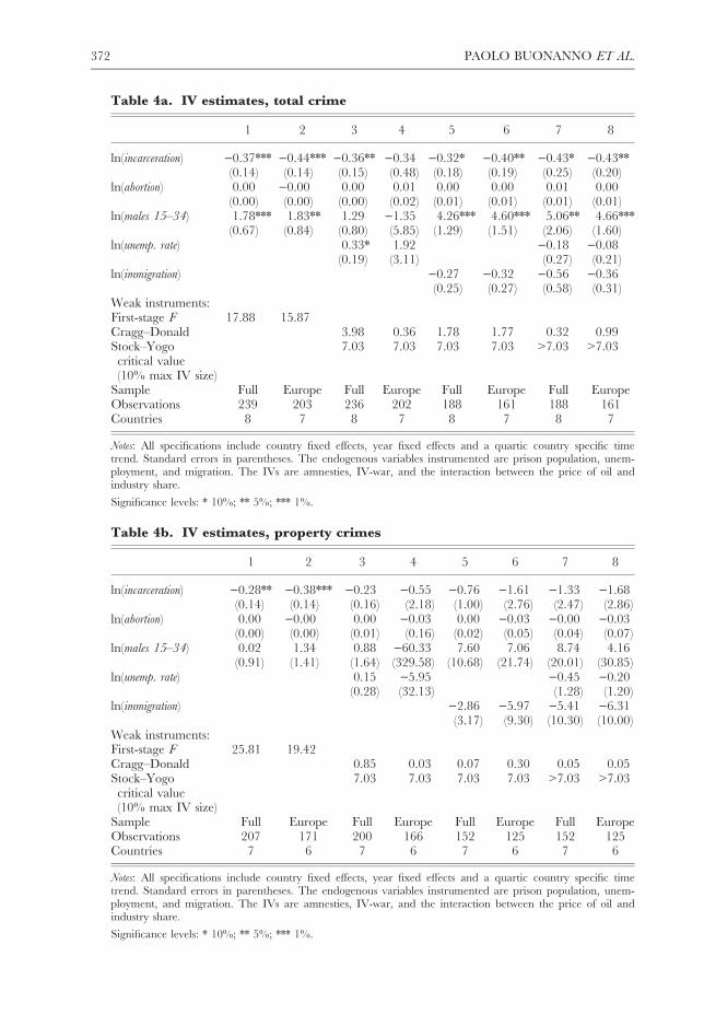
Table 4a. IV estimates, total crime

1 2 3 4 5 6 7 8

ln(incarceration) )0.37*** )0.44*** )0.36** )0.34 )0.32* )0.40** )0.43* )0.43**(0.14) (0.14) (0.15) (0.48) (0.18) (0.19) (0.25) (0.20)

ln(abortion) 0.00 )0.00 0.00 0.01 0.00 0.00 0.01 0.00(0.00) (0.00) (0.00) (0.02) (0.01) (0.01) (0.01) (0.01)

ln(males 15–34) 1.78*** 1.83** 1.29 )1.35 4.26*** 4.60*** 5.06** 4.66***(0.67) (0.84) (0.80) (5.85) (1.29) (1.51) (2.06) (1.60)

ln(unemp. rate) 0.33* 1.92 )0.18 )0.08(0.19) (3.11) (0.27) (0.21)

ln(immigration) )0.27 )0.32 )0.56 )0.36(0.25) (0.27) (0.58) (0.31)

Weak instruments:First-stage F 17.88 15.87Cragg–Donald 3.98 0.36 1.78 1.77 0.32 0.99Stock–Yogocritical value(10% max IV size)

7.03 7.03 7.03 7.03 >7.03 >7.03


Notes: All specifications include country fixed effects, year fixed effects and a quartic country specific timetrend. Standard errors in parentheses. The endogenous variables instrumented are prison population, unem-ployment, and migration. The IVs are amnesties, IV-war, and the interaction between the price of oil andindustry share.


Table 4b. IV estimates, property crimes

1 2 3 4 5 6 7 8

ln(incarceration) )0.28** )0.38*** )0.23 )0.55 )0.76 )1.61 )1.33 )1.68(0.14) (0.14) (0.16) (2.18) (1.00) (2.76) (2.47) (2.86)

ln(abortion) 0.00 )0.00 0.00 )0.03 0.00 )0.03 )0.00 )0.03(0.00) (0.00) (0.01) (0.16) (0.02) (0.05) (0.04) (0.07)

ln(males 15–34) 0.02 1.34 0.88 )60.33 7.60 7.06 8.74 4.16(0.91) (1.41) (1.64) (329.58) (10.68) (21.74) (20.01) (30.85)

ln(unemp. rate) 0.15 )5.95 )0.45 )0.20(0.28) (32.13) (1.28) (1.20)

ln(immigration) )2.86 )5.97 )5.41 )6.31(3.17) (9.30) (10.30) (10.00)


7.03 7.03 7.03 7.03 >7.03 >7.03





4.2. IV estimates

Tables 4a–4c report IV (2SLS) estimates, paralleling the OLS estimates reported in

Tables 3a–3c. Checking the strength of the instruments is crucial, because a weak

instrument may induce a bias similar to the OLS bias and reduce efficiency at the

same time. In the case of a single endogenous variable (i.e. columns 1 and 2), the

appropriate test is the standard first-stage F test on excluded instruments. The test

shows that amnesties, with an F well above 10, are a remarkably strong instrument.

First-stage estimates (not reported) indicate that the average effect of an amnesty in

our sample is to reduce the incarceration rate by about 13% in the year the

amnesty is passed. However, with n > 1 endogenous variables and n instruments

we have n first-stage regressions. In this case the rule of thumb formalized by Stai-

ger and Stock (1997) – that is, F >10 – can no longer be applied, and the appropri-

ate test is the one developed by Stock and Yogo (2002). This is a generalization of

the univariate F test on excluded instruments to the multivariate case, based on the

Cragg–Donald statistics. As a benchmark to interpret the magnitude of the

Cragg–Donald statistics, notice that this is approximately equal to the first-stage

F statistic on excluded instruments in the case of a single endogenous variable. The

Stock–Yogo test immediately reveals that the instrument for unemployment and

(even more) the instrument for immigration are very weak: we can never reject the

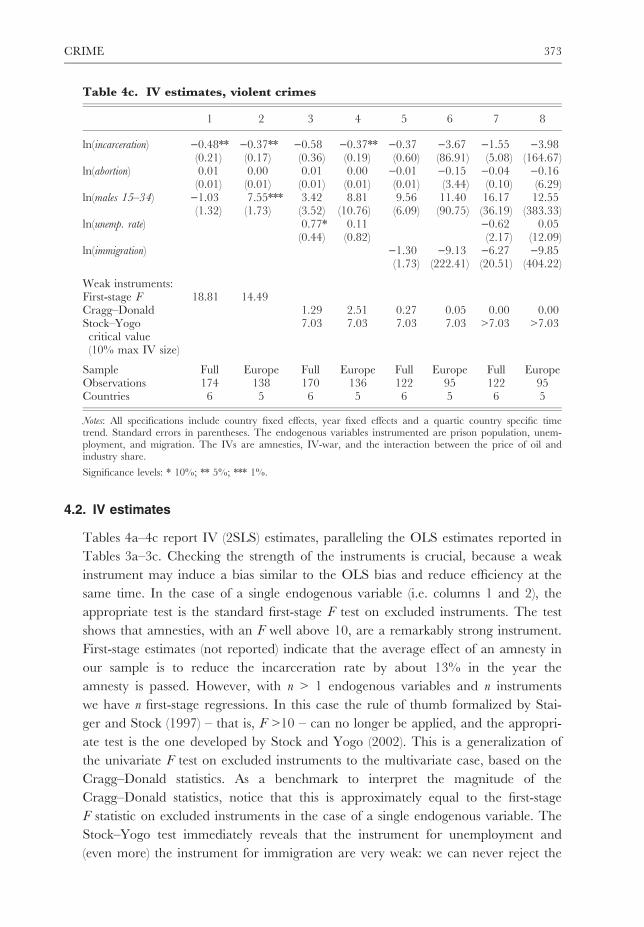
Table 4c. IV estimates, violent crimes

1 2 3 4 5 6 7 8

ln(incarceration) )0.48** )0.37** )0.58 )0.37** )0.37 )3.67 )1.55 )3.98(0.21) (0.17) (0.36) (0.19) (0.60) (86.91) (5.08) (164.67)

ln(abortion) 0.01 0.00 0.01 0.00 )0.01 )0.15 )0.04 )0.16(0.01) (0.01) (0.01) (0.01) (0.01) (3.44) (0.10) (6.29)

ln(males 15–34) )1.03 7.55*** 3.42 8.81 9.56 11.40 16.17 12.55(1.32) (1.73) (3.52) (10.76) (6.09) (90.75) (36.19) (383.33)

ln(unemp. rate) 0.77* 0.11 )0.62 0.05(0.44) (0.82) (2.17) (12.09)

ln(immigration) )1.30 )9.13 )6.27 )9.85(1.73) (222.41) (20.51) (404.22)


7.03 7.03 7.03 7.03 >7.03 >7.03




CRIME 373

null hypothesis of weak instruments when including either of these two variables.

The coefficients (and all coefficients) from specifications including these two vari-

ables are therefore unreliable as estimates of causal effects: even if the exclusion

restrictions hold the point estimates are not credible because the model is very

weakly identified. This also leads to very imprecise point estimates. An additional

reason for this imprecision is that data on immigration are available only from

1980 onwards: when using them, we lose about 30% of the observations. Similar

specifications (not reported) with a single endogenous regressor (either immigration

or unemployment) confirm the weakness of these two instruments: the first-stage

F statistic in this case is equal to 1.5 (immigration) and 5 (unemployment). The only

specification that provides credible causal effects is, therefore, the one in columns

1–2 of Tables 4a–4c, where in addition to identifying the elasticity of crime to

incarceration we identify the causal effect of abortion and age structure. This is our

preferred specification both because it avoids weak instruments issues and because

it considers the three factors (incarceration, abortion and age structure) that accord-

ing to Levitt (2004) and Imrohoroglu et al. (2004) are among the main factors

behind the drop in crime rates in the United States in the 1990s.

We deliberately choose to include in the regression only plausibly exogenous

variables (or instrumented endogenous variables). For example, despite the fact the

real GDP per-capita is strongly correlated to all economic fundamentals that,

according to the standard economic model of crime, potentially affect crime (e.g.

poverty, business cycle, property rights, human development, and even happiness),

this is not included in our regressions because it is potentially endogenous to crime

rates. It is worth noting, however, that our results are essentially unchanged when

we include GDP as a control. This is illustrated in the Web Appendix.

In the remainder of this section we discuss the estimates from our preferred spec-

ification in more detail.

4.2.1. Incarceration. As mentioned above, first-stage estimates (not reported) indi-

cate that the effect of amnesties on the prison population is large and significant.

Passing one amnesty in one year leads to a reduction in the prison population

rate of about 13% in our preferred specification. Comparing the estimates on incar-

ceration in Tables 3 and 4, most of the OLS coefficients are generally lower than

the corresponding IV, suggesting that OLS underestimate the effect of the prison

population on crime, as expected. The exception is the elasticity of property crime

to incarceration, which turns out to be upward biased when using OLS. Table-

s 4a–4c show that the elasticity of total crime per capita to the incarceration rate,

using IV in our preferred specification, is )0.37 for the full sample and )0.44 for

Europe only. A similar pattern is found for property crime ()0.28 for the full sample

and )0.38 for Europe only) and for violent crime ()0.48 for the full sample and

)0.37 for Europe only). As discussed above, superimposing a quartic country-specific

trend is a conservative approach: in fact, had we not employed such trends the coef-


ficients on incarceration rates would have been larger, except for violent crimes (see

Web Appendix). Furthermore, our estimate of the effect of incarceration is robust to

excluding abortion and demographics from the regression (results not reported). This

robustness confirms the presumption that amnesties do provide a source of exoge-

nous variation for incarceration rates. Overall, our results on incarceration are in

line with previous estimates by Levitt (1996), who exploits overcrowding litigation

across US states as an instrument and finds an elasticity in the range )0.3 to )0.4.

We perform a simple back-of-the-envelope calculation to quantify the contribu-

tion of the prison population to the ‘reversal of misfortunes’. The calculation works

as follows. Start with the crime rates in Europe and in the United States in 1970,

and simulate the dynamics of crime using incarceration as the only explanatory var-

iable, with the elasticities reported in the first column of Table 4a, 4b, 4c. Then

compare the simulated difference between crime rates in 2008 and in 1970 with

the actual difference. The ratio of the two is the contribution of the different

dynamics of prison population to the reversal. This calculation reveals that incar-

ceration explains 17% of the reversal for total crime, 33% for property crimes

alone, and 11% for violent crimes alone.

4.2.2. Abortion rates. As Tables 3 and 4 show, we do not find evidence supporting

the hypothesis that abortion rates decrease crime rates as Donohue and Levitt

(2001) find for the United States. Most of the point estimates have a positive sign

(which is the ‘wrong sign’) and are not precisely estimated. It is likely that the quar-

tic time trend absorbs all the variation in abortion rates, a slow-moving variable like

the demographic structure of the population. In fact when we remove the time

trend or use a linear trend we obtain a negative and significant point estimate (see

Web Appendix). However, even in this case the effect of abortion on crime rates

disappears when we consider European countries only (not reported). A word of

caution, however, is in order when comparing our findings with those of Donohue

and Levitt. As mentioned above, their measure of abortion rates is computed as the

sum of the abortion rate of each age group weighted by the percentage of arrests

in a cohort over the total crime in the United States in a given year. This measure

captures what they call the effective abortion rate, that is, the measure that is rele-

vant to crime in a given year. For European countries, data on arrests for each

cohort are not readily available every year so that we can only use the unweight-

ed abortion rates in our analysis. It is interesting, though, that the significant point

estimate obtained when removing time trends or using linear trends is completely

driven by the United States. A possible explanation is that in Europe a strong

welfare state, easy access to good education and strong family ties work as risk-

reducing factors that weaken the link between unwanted childbearing and crime.

Overall, one of the key elements explaining the drop in crime rates in the United

States seems to be ineffective in Europe. This result certainly deserves further

research.

CRIME 375

4.2.3. Age structure. The elasticity of crime to the weight of young males in the

population is about 1.5 (IV estimates, preferred specification) and it is slightly larger

for European countries. Keeping constant the population, an increase of 1% in the

share of males between 15 and 34 years of age leads to a 1.5% increase in the total

crime rate. This effect is imprecisely estimated when we use property crimes as a

dependent variable. As for violent crimes, we obtain a very large estimate for the

European group in isolation. While a large coefficient for violent crime is not sur-

prising, a point estimate of 7 seems quite large. The same back-of-the-envelope cal-

culation made for incarceration rates suggests that the different dynamics in the age

structure between European countries and the United States cannot explain the

reversal of misfortune, a fact that was already made clear by Figure 4.

5. CONCLUDING REMARKS

In this paper we have explored the evolution of crime rates in Europe and in the Uni-

ted States since 1970. We have documented a ‘reversal of misfortunes’ and have

attempted the identification of the causes of this reversal. We have estimated the

impact of demographic structure, incarceration and abortion on crime rates. Unfortu-

nately, due to weak instruments, we cannot provide reliable evidence on the causal

effects of migration and unemployment rates. The OLS estimates for these two vari-

ables suggest that migration and unemployment increase crime rates, but it is not pos-

sible to assess the OLS bias. We uncovered two significant causal channels, though:

both the demographic structure of the population and the incarceration rate have a

non-negligible influence on crime rates. Back-of-the-envelope calculations based on

our estimates indicates that the different dynamics of the prison populations in Eur-

ope and the United States explain 17% of the reversal of misfortunes for total crime,

33% for property crimes, and 11% for violent crimes. We do not find evidence that

abortion rates reduce crime rates in Europe as much as previously found for the Uni-

ted States. Understanding why is beyond the scope of this paper, but future research

should investigate this different response of crime rates to abortion in Europe.

On the methodological side, we are well aware of the limitations of our analysis.

We acknowledge them here to emphasize that we regard our empirical exercise as

a starting point for further research rather than a conclusive word on an admittedly

complicated question. First, as Durlauf et al. (2008, 2010) show, aggregate crime

regressions like those used in this paper are consistent with a benchmark micro-

structure only under strong assumptions about the distribution of unobserved indi-

vidual heterogeneity. This points to a second limitation, namely the use of a

reduced-form approach that mimics experimental variations via instrumental vari-

ables to uncover causal effects. There is much controversy about what policymakers

can learn from such exercises (see, for instance, the Journal of Economic Perspectives,

Spring 2010, symposium on ‘Con out of economics’). We regard such controversy

as a constructive step towards a better empirical economics. In the meanwhile we


warn readers that our results are to be taken with caution, because the reduced

form approach we adopt is not able to pin down the channel through which the

factors that we analyse influence crime rates. Furthermore, reduced-form parame-

ters are likely not policy-invariant. As a consequence, it is difficult to make reliable

out-of-sample predictions. Third, there is no consensus on the use of time trends in

policy evaluation exercises (see, for instance, the discussions in Wolfers, 2006, and

Durlauf et al., 2008). We have shown that a quartic trend is a reasonable choice for

the problem at hand. However, this remains a matter of judgment. Finally, we con-

sider a selected set of explanatory variables. While the five factors we consider are

those emphasized in the economics literature on crime, we have no framework dic-

tating that these and only these should be considered.

What are the policy implications of our analysis? The first main finding – that is,

the existence of a reversal – should make policymakers in Europe aware of the fact

that crime (and violent crime in particular) is a very relevant issue, more than we

are accustomed to thinking when making casual comparisons with the United

States. The fact that the homicide rate is much higher in the United States than

in Europe (as documented in the Web Appendix) seems to generate the wrong

perception that Europe is a safer place. But homicides are only a small fraction

(although very important for their consequences) of violent crimes. The second main

finding – an elasticity of crime to incarceration of )0.4 – implies that incarceration

works. Therefore, a tougher incarceration policy may be an effective way of reduc-

ing crime in Europe. While this causal effect is informative, it raises two issues. First,

without knowing why incarceration works, it is hard to decide in what sense incar-

ceration policy should be tougher. If it works because of incapacitation, then con-

victing more criminals to longer sentences is the sense in which the policy should be

tougher. But if incarceration works because of deterrence, then inflicting long sen-

tences and placing criminals on parole, for instance, would be better policy. It is

impossible to resolve this first issue in a reduced-form framework like the one we

have employed: more research is needed on the channels that make incarceration

work. Second, our finding that incarceration is crime-effective does not imply that it

is a cost-effective policy. To conclude that more incarceration or longer sentences

are needed in Europe, we should understand how, at the current incarceration rates,

the marginal cost of a prison inmate to society compares to the marginal cost of

crime to victims in Europe. If the cost (to society) of incarcerating an additional

individual is below the cost (to victims) of additional crimes that this individual

would commit if left free, then more incarceration is efficient. For this type of cost-

benefit analysis, one needs two parameters: the elasticity of crime to incarceration

and the marginal costs of both crime and incarceration. In this paper we estimate

the first parameter. Calculating the marginal cost of crime and of incarceration is

hard because it involves things that are difficult to estimate. For instance, recent

research shows that incarceration may have a criminogenic effect on recidivism in

the long run (e.g. Chen and Shapiro, 2007; Bayer et al., 2009; Nagin et al., 2009;

CRIME 377

Drago et al., 2011). Such dynamic, general equilibrium effects are not captured by

our estimates (which are based on a static panel data model) and may crucially alter

cost-benefit calculations. In particular, they may increase the marginal cost of incar-

ceration. Moreover, the ‘cost of an inmate to society’ includes not only the direct cost

of incarceration, but also the indirect costs in terms of additional general equilibrium

effects, from the distortionary effects of taxation needed to finance the judiciary and

prison systems to the effects on labour market equilibrium. This does not mean that

the cross-country evidence we have produced is of little use: while these two outstand-

ing issues prevent us from drawing strong policy conclusions, our estimates are quite

relevant for crime policy because they provide the basis to understand if more incar-

ceration in Europe would be efficient. But more research on this point is needed.

Discussion

Jerome AddaUniversity College London

This is a careful and interesting analysis that brings for the first time comparable

data across Europe and the US on various types of crime and its determinants.

The authors have made great effort to investigate the causal effect of many deter-

minants of crime. However, I even found the descriptive statistic of great interest.

The authors concentrate on five determinants of crime, which the previous

literature has identified as important. These include demographics, immigration,

unemployment, incarceration rates and abortion rates. The study leaves out other

determinants such as the role of education and the differential timing of drug waves

(such as crack-cocaine). The role of education in shaping crime has been investi-

gated by Lochner and Moretti (2004) among others. Presumably, the authors have

left out this variable for lack of reliable data across countries for the period of ana-

lysis. The authors control for GDP per capita as a measure of income. However,

what may be important are changes in the unskilled wage or minimum wage

(Machin and Meghir 2004). Another determinants of crime, or at least of its cycli-

cality, could be selective fertility induced by business cycles (as described by Dehejia

and Lleras-Muney 2004). As with selective abortion, it could change the composi-

tion of the young population. The strength of the paper is in its use of instrumental

variables to deal with the endogeneity of some of the explanatory variables. The

validity of this procedure relies on the quality of these instruments. While I have lit-

tle problem with the supply-push factors to explain migration, other instruments

requires stronger assumptions. For instance, amnesties are used to instrument incar-

cerations. The authors do a great job to show that amnesties are not correlated

with past crime. However, is it politically feasible to pass an amnesty when current

crime is high or its growth rate is high? Moreover, during amnesty, the most dan-


gerous criminals are usually not pardoned. What this exercise estimates is the effect

of releasing low-level criminals, not a random selection of offenders. Finally, as

usual in this literature, the incarceration variable is measuring both a deterrence

effect and a lock-in effect. Distinguishing between both channels would be an inter-

esting exercise, although beyond the scope of this paper.

Bas JacobsErasmus University Rotterdam

This is an interesting paper on a policy-relevant and under-researched topic. The

paper is well structured and the analysis is straightforward, transparent and clear.

The authors document that crime rates in Europe have become much higher than

in the US since 1990. In the US, crime rates substantially dropped during the last

20 years. The authors present a well-executed empirical analysis on the determi-

nants of crime in Europe so as to explain this divergent EU-US crime pattern.

Their main finding is that crime rates can be causally explained by incarceration

rates and the fraction of the male population aged 15-34. They find that the elasti-

city of crime with respect to incarceration rates for EU-countries is about the same

size as estimates obtained for the US. The authors use quite a convincing identifica-

tion strategy by resorting to prison amnesties to generate exogenous variation in

incarceration rates. Similarly, the authors assume quite reasonably that demo-

graphic variation is exogenous. Moreover, the authors demonstrate that unemploy-

ment (instrumented with oil-prices) and migration flows (instrumented with civil

and ethnic wars or ethnic violence) have little explanatory power to explain crime

rates. A number of comments can be made regarding the paper. Although appar-

ently often suggested in the crime literature, it is not so obvious that immigration

should have an impact on crime. One may suspect that there is a large amount of

heterogeneity in the immigrant population, ranging from asylum seekers, family

reunification, to labor migrants. Heterogeneity among immigrants is also caused by

country of origin, income levels and skill levels. Moreover, within the EU there is

free migration accounting for 27 percent of total immigration in the OECD and 44

percent of immigration in the EU-area (OECD, 2010). Probably, illegal immigrants

are overrepresented in crime statistics, but the latter group is not captured by the

official migration statistics, which are employed in the current paper. Similarly, it

would be surprising that labor immigration (including migration of spouses) – which

covers about 17 percent of total OECD-immigration – would be strongly associated

with crime, since migrants obtain a visa only conditional upon having work. Simi-

larly, family reunification – accounting for 18 percent of total OECD-immigration –

is possible only when certain age and income requirements are met. The figures

are drawn from OECD (2010). Hence, one should be careful in presuming that

immigration and crime are intimately linked. In addition, definitions of migration

stocks can vary across countries due to differences in the definition of who is

CRIME 379

considered to be an immigrant. The paper and the web appendix do not provide

details on the way migration stocks are measured and whether the data are com-

parable across countries and over time. For all these reasons, a weak correlation

between crime and immigration might not be surprising in the first place. Using

weak instruments for migration tends to weaken this correlation even further. The

authors are aware of potential shortcomings of their empirical strategy. In particu-

lar, they are very clear about the strength of the instruments they employ to obtain

exogenous variation in the explanatory variables. I would have liked them having

tried improving this part of the paper and to obtain more reliable instruments for

the unemployment and migration variables. As regards unemployment, the authors

follow Blanchard and Katz (1992) by using oil-prices to generate exogenous varia-

tion in unemployment rates. The instrument does not seem to work very well, per-

haps because there is no cross-country variation in oil-prices and little time-

variation in sectoral structure across countries. As an alternative instrument, one

could possibly look at how changes in world trade affect employment in European

countries. Most EU-countries are small-open economies that have a limited (if not

negligible) impact on world-trade. If one believes that world-trade is exogenous to

small-open economies, then this could be a reasonable variable to instrument

unemployment rates. Cross-country variation can be introduced by interacting

world-trade with the openness of a country. Similarly, numerous European coun-

tries have implemented structural labor market reforms in recent decades. Argu-

ably, these reforms were not implemented to reduce crime rates, but to reduce

structural unemployment. Therefore, dummy variables indicating whether there

have been structural reforms in labor markets could be suitable instruments for

unemployment as well. As regards immigration, the authors should be applauded

for compiling their own data set with variables based on civil war, ethnic war or

ethnic violence. Unfortunately, these instruments also appear weak in explaining

migration patterns, as also indicated by the authors. I wonder whether this is due

to the fact that migration flows predicted by these variables presumably mainly

reflect asylum seekers. Asylum seekers are not representative for migrant popula-

tions in many countries. Asylum migration accounts for only 5 percent of total

OECD-migration (OECD, 2010). Immigration flows are also determined by, for

example, free movement of individuals in the EU, labor migration, marriage and

family reunification. These immigration flows are not so much caused by war or

violence, but by, among others, colonial and guest-worker histories and the Schen-

gen Treaty. Hence, the instrument cannot capture a lot of the variation in migra-

tion flows. A suggestion is then to seek for instruments that relate to e.g.

colonization patterns decades or even hundreds of years ago to predict current

migration flows. Similarly, many countries have adopted guest-worker policies in

the 1950s and 1960s when large numbers of guest workers were recruited. Vari-

ables related to guest-worker migration decades ago could therefore be reasonable

instruments for current migration flows, since current crime rates are arguably not


caused by colonial and guest-worker histories. Finally, the introduction of the

Schengen Treaty could be exploited as a natural experiment to generate exogenous

variation in migration flows. The paper documents a very intriguing pattern in the

crime rates in Europe and the US; Europe has overtaken the US in crime since the

1990’s. The authors take a first step in explaining this pattern using a number of

explanatory variables suggested by the literature: demographics, incarceration rates,

abortion rates, migration rates and unemployment rates. However, only the demo-

graphic and incarceration variables appear to be causally explaining crime. For

future research, one should probably explore other variables to explain crime as

well, such as income (growth), drug-related activities, family and social problems,

psychological traits, etc. However, one should be careful not to replicate research

that is already done in, for example, criminology, psychology or sociology. As it

seems, the time-series pattern in crime in the US and Europe discussed in the cur-

rent paper appears to be well-known in criminology, see, for example, PEW Center

on the States (2008). Finally, the policy conclusion is reached that higher incarcera-

tion rates are beneficial in reducing crime. I would like to raise a word of caution

against policies explicitly aiming to raise the total incarceration rate. Police officers

often say that prison provides the best education for a career in crime. In the

short-run, higher incarceration rates could indeed reduce crime, either through

deterrence or through incapacitation. However, the long-run effect could be that

the stock of ‘criminal human capital’ grows and an ever increasing number of indi-

viduals need to be incapacitated to prevent them from committing new crimes.

The US seems to have had exactly this experience, as the current US-incarceration

rate is about five times bigger than 40 years ago, about 7.2 million individuals were

under some form of correctional supervision (probation, prison, jail, parole), and

more than half of released offenders went back to prison within three years (Bureau

of Justice Statistics, 2011).

Panel discussion

Volker Nocke wondered whether there was any change in the composition of the

prisoner cohort in countries over time. He speculated that in East European coun-

tries there is a high level of organized crime and many of these people facilitated

by European Union accession may now operate in other European countries. Dalia

Marin referred the authors to previous research which argued that an important

determinant of crime among young males was their marriage status. Findings in a

Quarterly Journal of Economics paper suggest that the introduction of the contraceptive

pill led to a decline in shotgun weddings which reduced the number of young men

with familial responsibilities and their need to commit crime in order to provide for

their family. Eric Hanushek noted that in the United States the average level of

CRIME 381

educational attainment has remained more or less constant while it has increased

across European countries. This would appear to contradict the claim that higher

levels of education reduce the crime rate.

Many of the panellists focused on specific aspects of the empirical strategy pur-

sued by the authors in the paper. Marco Pagano believed that the oil shocks vari-

able was not a good instrument for unemployment as it was likely to explain only a

small percentage of its variation and urged them to search for alternative instru-

ments. Michael Kiley advised the authors to continue with their instrumenting

strategy. Even though their instruments are found to be weak they may still

uncover robust findings. Andrea Ichino believed their approach is useful for under-

standing the differences in the crime rates between the United States and Europe;

however analysis of individual country amnesty events could provide specific

insights into the effect of incarceration on crime which would better inform policy.

Some of the panellists believed that many of the country-level determinants of

crime such as abortion rates to be relatively stable over the time period analysed.

The inclusion of fixed effects eliminated much of the variation in these variables

and therefore the likelihood of identifying their effect on crime. Fabrizio Perri

believed unemployment and immigration are more important determinants of

crime than the analysis suggests. He suggested the authors should estimate country-

specific regressions and also estimate their pooled regressions without time trends to

see if the effects of unemployment and immigration become more meaningful. Re-

fet Gurkaynak focused on the role of the large downward trend in the US crime

rate in the data. He suggested that a US specific regression was likely to yield insig-

nificant results. He wondered how much of the current variation in the main model

was explained by the inclusion of the United States.

Richard Portes wondered if there is any research on the link between the age at

which alcohol can be legally consumed and violent crime. He also made the point

that the large proposed budget cuts in the United Kingdom include a substantial

cut to the prison budget and is likely to lead to a reduction in the incarceration

rates which would provide an interesting experiment on the link with crime rates.

Given there are higher crimes rates in cities, Daniele Terlizzese wondered if the

authors had considered the structure of cities as an explanation for the larger crime

rate in Europe compared to the United States.

In response to comments by Fabrizio Perri and other panellists, Giulio Zanella

remarked that they adopted a conservative approach to ensure the robustness of the

identified effect of incarceration on crime. In model estimations without quadratic

time trends they find that a number of the demographic variables become significant,

the effect of abortion on crime remains insignificant while the incarceration coeffi-

cient is higher. In reply to Eric Hanushek’s comment, Giulio Zanella agreed it was

important to control for education attainment; however, the variable is likely to be

endogenous with crime rates and they would need to find another instrument.


Web appendix

Available at http://www.economic-policy.org.

REFERENCES (INCLUDING REFERENCES FOR THE WEB APPENDIX)

Angrist, J. and A. Kugler (2003). ‘Protective or counter-productive? Labour market institu-tions and the effect of immigration on EU natives’, Economic Journal, 113(488), 302–31.

Barbarino, A. and G. Mastrobuoni (2008). ‘The incapacitation effect of incarceration: Evi-dence from several Italian collective pardons’, mimeo, Collegio Carlo Alberto Torino.

Bayer, P., R. Hjalmarsson and D. Pozen (2009). ‘Building criminal capital behind bars’,Quarterly Journal of Economics, 124(1), 105–47.

Becker, G. (1968). ‘Crime and punishment: An economic approach’, Journal of Political Econ-omy, 76, 169–217.

Bianchi, M., P. Buonanno and P. Pinotti (2011). ‘Do immigrants cause crime?’ Journal of theEuropean Economic Association, forthcoming.

Blanchard, O. and L. Katz (1992). ‘Regional evolutions’, Brookings Papers on Economic Activity,1, 1–75.

Blumstein, A. and J. Wallman (2000). The Crime Drop in America. Cambridge University Press,Cambridge.

Borjas, G., J. Grogger and G. Hanson (2010). ‘Immigration and the economic status of Afri-can-American men’, Economica, 77, 255–82.

Buonanno, P., D. Montolio and P. Vanin (2009). ‘Does social capital reduce crime?‘ Journalof Law and Economics, 52(1), 145–70.

Bureau of Justice Statistics (2011), http://bjs.ojp.usdoj.gov/.Butcher, K. and A. Piehl (1998a). ‘Cross-city evidence on the relationship between immigra-

tion and crime’, Journal of Policy Analysis and Management, 17(3), 457–93.—— (1998b). ‘Recent immigrants: Unexpected implications for crime and incarceration’,

Industrial and Labor Relations Review, 51(4), 654–79.—— (2005). ‘Why are immigrants’ incarceration rates so low? Evidence on selective immi-

gration, deterrence, and deportation’, Federal Reserve Bank of Chicago Working PaperWP-05-19.

Card, D. (1990). ‘The impact of the Mariel boatlift on the Miami labor market’, Industrialand Labor Relations Review, 43(2), 245–57.

—— (2001). ‘Immigrant inflows, native outflows, and the local labor market impacts ofhigher immigration’, Journal of Labor Econonomics, 19(1), 22–64.

—— (2009). ‘Immigration and inequality’, American Economic Review, 99(2), 1–21.Chen, K. and J. Shapiro (2007). ‘Do harsher prison conditions reduce recidivism? A discon-

tinuity-based approach’, American Law and Economic Review, 9, 1–29.Cook, P. and N. Khmilevska (2005). ‘Cross-national patterns in crime rates’, Crime and Jus-

tice, 33, 331–46.Cook, P. and J. Laub (2002). ‘After the epidemic: Recent trends in youth violence in the

United States’, in M. Tonry (ed.), Crime and Justice: A Review of Research, University of Chi-cago Press, Chicago, 117–53.

Cortes, P. (2008). ‘The effect of low-skilled immigration on U.S. prices: Evidence from CPIdata’, Journal of Political Economy, 116(3), 381–422.

Dehejia, Rajeev and Adriana Lleras-Muney (2004). ‘Booms, busts, and babies’ health’, Quar-terly Journal of Economics, 119(3), 1091–1130.

Donohue, J. and S. Levitt (2001). ‘The impact of legalized abortion on crime’, Quarterly Jour-nal of Economics, 116(2), 379–420.

—— (2004). ‘Further evidence that legalized abortion lowered crime: A reply to Joyce’, Jour-nal of Human Resources, 39(1), 29–49.

—— (2008). ‘Measurement error, legalized abortion, and the decline in crime: A response toFoote and Goetz’, Politics & the Life Sciences, 123(1), 425–40.

CRIME 383

Donohue, J., J. Grogger and S. Levitt (2009). ‘The impact of legalized abortion on teenchildbearing’, American Law and Economics Review, 11(1), 24–46.

Draca, M., S. Machin and R. Witt (2010). ‘Panic on the streets of London: Police, crimeand the July 2005 terror attacks’, American Economic Review, forthcoming.

Drago, F. and R. Galbiati (2010). ‘Indirect effects of a policy altering criminal behaviour:Evidence from the Italian prison experiment’, IZA Discussion Paper No. 5414.

Drago, F., R. Galbiati and P. Vertova (2009). ‘The deterrent effects of prison: Evidencefrom a natural experiment’, Journal of Political Economy, 117(2), 257–80.

—— (2011). ‘Prison conditions and recidivism’, American Law and Economics Review, forthcom-ing.

Durlauf, S., S. Navaro and D. Rivers (2008). ‘On the use of aggregate crime regressions inpolicy evaluation’, in Understanding Crime Trends: Workshop Report, The National Academy ofScience.

—— (2010). ‘Understanding aggregate crime regressions’, Journal of Econometrics, 158,306–17.

Ehrlich, I. (1973). ‘Participation in illegitimate activities: A theoretical and empirical investi-gation’, Journal of Political Economy, 81(3), 521–65.

Foote, C. and F. Goetz (2008). ‘The impact of legalized abortion on crime: Comment’,Quarterly Journal of Economics, 123, 1.

Fougere, D., F. Kramarz and J. Pouget (2009). ‘Youth unemployment and crime in France’,Journal of the European Economic Association, 7(5), 909–38.

Gould, E., B. Weinberg and D. Mustard (2002). ‘Crime and local labor market opportuni-ties in the United States: 1979–1997’, The Review of Economics and Statistics, 87(3), 411–22.

Home Office (2008). ‘Crime in England and Wales 2007/08. Findings from the BritishCrime Survey and police recorded crime’, Home Office Statistical Bulletin, July.

Imrohoroglu, A., A. Merlo and P. Rupert (2004). ‘What accounts for the decline in crime?‘International Economic Review, 3(8), 707–29.

Jaeger, D. (2006). ‘Green cards and the location choices of immigrants in the United States,1971–2000’, IZA Discussion Paper No. 2145

Joyce, T. (2004). ‘Did legalized abortion lower crime?‘ Journal of Human Resources, 39(1),1–28.

Kahane, L., D. Paton and R. Simmons (2007). ‘The abortion-crime link: Evidence fromEngland and Wales’, Economica, 75(297), 1–21.

Levitt, S. (1996). ‘The effect of prison population size on crime rates: Evidence from prisonovercrowding litigation’, Quarterly Journal of Economics, 111 (May), 319–51.

—— (2004). ‘Understanding why crime fell in the 1990s: Four factors that explain the de-cline and six that do not’, Journal of Economic Perspectives, 18(1), 163–90.

Levitt, S. and L. Lochner (2001). ‘The determinants of juvenile crime’, in Risky Behavioramong Youths: An Economic Analysis, National Bureau of Economic Research, 327–74.

Levitt, S. and T. Miles (2007). ‘Empirical study of criminal punishment’, in A. M. Polinsky an-d S. Shavell (eds.), Handbook of Law and Economics, vol. 1, North-Holland, Amsterdam.

Lin, M. (2008). ‘Does unemployment increase crime? Evidence from U.S. data 1974–2000’,Journal of Human Resources, 43(2), 413–36.

MacDonald, Z. (2002). ‘Official crime statistics: Their use and interpretation’, Economic Jour-nal, 112(477), F85–F106.

Machin, Stephen, Meghir and Costas (2004) ‘‘Crime and Economic Incentives’’, Journal ofHuman Resources 2004 XXXIX: 958–979.

McKenzie, D. and H. Rapoport (2007). ‘Self-selection patterns in Mexico-U.S. migration:The role of migration networks’, CReAM Discussion Paper No. 0701.

Moehling, C. and A. Piehl (2007). ‘Immigration and crime in early 20th century America’,NBER Working Paper No. 13576.

Moretti E. and L. Lochner (2004) ‘‘The Effect of Education on Criminal Activity: Evidencefrom Prison Inmates, Arrests and Self-Reports’’ American Economic Review 94(1).

Munshi, K. (2003). ‘Networks in the modern economy: Mexican migrants in the U.S. labormarket’, Quarterly Journal of Economics, 118(2), 549–99.

Murphy, K. and F. Welch (1990). ‘Empirical age-earnings profiles’, Journal of Labor Economics,8(2), 202–29.


Nagin, D., F. Cullen and C. Lero Johnson (2009). ‘Imprisonment and reoffending’, Crimeand Justice, 38, 115–200.

OECD (2010), ‘‘International Migration Outlook’’, Paris: OECD.Oster, A. and J. Agell (2007). ‘Crime and unemployment in turbulent times’, Journal of the

European Economic Association, 5(4), 752–75.Ottaviano, G. and G. Peri (2006). ‘The economic value of cultural diversity: Evidence from

US cities’, Journal of Economic Geography, 6(1), 9–44.PEW Center on the States (2008), ‘‘The Impact of Incarceration on Crime’’, Expert Q&A

No. 5, 2008.Pop-Eleches, C. (2006). ‘The impact of a change in abortion regime on socio-economic out-

comes of children: Evidence from Romania’, Journal of Political Economy, 114(4), 744–73.Raphael, S. and R. Winter-Ebmer (2001). ‘Identifying the effect of unemployment on

crime’, Journal of Law & Economics, 44(1), 259–83.Saiz, A. (2007). ‘Immigration and housing rents in American cities’, Journal of Urban Econom-

ics, 61(2), 345–71.Soares, R. (2004). ‘Development, crime and punishment: Accounting for the international

differences in crime rates’, Journal of Development Economics, 73, 155–84.Staiger, D. and J. Stock (1997). ‘Instrumental variables regression with weak instruments’,

Econometrica, 65, 557–86.Stock, J. and M. Yogo (2002). ‘Testing for weak instruments in linear IV regression’, NBER

Technical Working Papers 0284.Van Dijk, J., J. Van Kesteren and P. Smit (2007). Criminal Victimisation in International Perspec-

tive, Wetenschappelijk Onderzoeken Documentatiecentrum.Wolfers, J. (2006). ‘Did unilateral divorce raise divorce rates? A reconciliation and new

results’, American Economic Review, 96(5), 1802–20.Zimring, F. (2006). The Great American Crime Decline, Oxford University Press, New York.

CRIME 385

Crime in Europe and the United States: dissecting the ‘reversal of misfortunes

Documents