Crime as Tourism Externality

CRIME AS TOURISM EXTERNALITY

Bianca Biagi Claudio Detotto

WORKING PAPERS

2 0 1 0 / 1 5

C O N T R I B U T I D I R I C E R C A C R E N O S

CUEC  

C E N T R O R I C E R C H E E C O N O M I C H E N O R D S U D

( C R E N O S ) U N I V E R S I T À D I C A G L I A R I U N I V E R S I T À D I S A S S A R I

I l C R E N o S è u n c e n t r o d i r i c e r c a i s t i t u i t o n e l 1 9 9 3 c h e f a c a p o a l l e U n i v e r s i t à d i C a g l i a r i e S a s s a r i e d è a t t u a l m e n t e d i r e t t o d a S t e f a n o U s a i . I l C R E N o S s i p r o p o n e d i c o n t r i b u i r e a m i g l i o r a r e l e c o n o s c e n z e s u l d i v a r i o e c o n o m i c o t r a a r e e i n t e g r a t e e d i f o r n i r e u t i l i i n d i c a z i o n i d i i n t e r v e n t o . P a r t i c o l a r e a t t e n z i o n e è d e d i c a t a a l r u o l o s v o l t o d a l l e i s t i t u z i o n i , d a l p r o g r e s s o t e c n o l o g i c o e d a l l a d i f f u s i o n e d e l l ’ i n n o v a z i o n e n e l p r o c e s s o d i c o n v e r g e n z a o d i v e r g e n z a t r a a r e e e c o n o m i c h e . I l C R E N o S s i p r o p o n e i n o l t r e d i s t u d i a r e l a c o m p a t i b i l i t à f r a t a l i p r o c e s s i e l a s a l v a g u a r d i a d e l l e r i s o r s e a m b i e n t a l i , s i a g l o b a l i s i a l o c a l i . P e r s v o l g e r e l a s u a a t t i v i t à d i r i c e r c a , i l C R E N o S c o l l a b o r a c o n c e n t r i d i r i c e r c a e u n i v e r s i t à n a z i o n a l i e d i n t e r n a z i o n a l i ; è a t t i v o n e l l ’ o r g a n i z z a r e c o n f e r e n z e a d a l t o c o n t e n u t o s c i e n t i f i c o , s e m i n a r i e a l t r e a t t i v i t à d i n a t u r a f o r m a t i v a ; t i e n e a g g i o r n a t e u n a s e r i e d i b a n c h e d a t i e h a u n a s u a c o l l a n a d i p u b b l i c a z i o n i . w w w . c r e n o s . i t i n f o @ c r e n o s . i t

C R E N O S – C A G L I A R I V I A S A N G I O R G I O 1 2 , I - 0 9 1 0 0 C A G L I A R I , I T A L I A

T E L . + 3 9 - 0 7 0 - 6 7 5 6 4 0 6 ; F A X + 3 9 - 0 7 0 - 6 7 5 6 4 0 2

C R E N O S - S A S S A R I V I A T O R R E T O N D A 3 4 , I - 0 7 1 0 0 S A S S A R I , I T A L I A

T E L . + 3 9 - 0 7 9 - 2 0 1 7 3 0 1 ; F A X + 3 9 - 0 7 9 - 2 0 1 7 3 1 2 T i t o l o : CR IME AS TOURISM EXTERNAL ITY I SBN: 978 88 84 67 596 5 P r ima Ed i z i one : Lug l i o 2010 © CUEC 2010 V i a I s M i r r i o n i s , 1 09123 C a g l i a r i T e l . / F a x 070 291201 w w w . c u e c . i t

1

Crime as tourism externality

Bianca Biagi Claudio Detotto

DEIR and CRENoS, University of Sassari

Abstract

This paper analyses the linkage between tourism and crime with particular focus on the distortions generated onto criminal activities by the presence of visitors. Controlling for socio-demographic and economic variables, we empirically investigate the contribution of tourist arrivals to different types of crimes for 103 Italian provinces and for the year 2005. Possible spill-over effects of crime are taken into account by testing two spatial models (one spatial lag model and one spatial error model). We also test the hypothesis according to which the different geography of tourist destinations - i.e. urban, mountain, marine etc- alters the impact of tourism on crime. Finally, we measure the social cost of crime associated with tourist arrivals. Keywords: Crime, tourism, spill-over effect, negative externality. JEL: L83; K0; R0.

2

1. Introduction In a tourist town in Italy, a professor of economics, his Belgian wife and their two

children are walking. A motorbike with two local boys slowly approaches them; suddenly the guy sitting behind the driver tries to snatch the bag from the wife. The professor shouts - in Italian - to leave the wife's bag. The two boys surprised by his perfect pronunciation ask the professor where he comes from, the professor replies that he is Italian and lives in the town. The two thieves then return the bag to the professor apologising to him and his wife, saying that they mistook them for tourists.1 In the last decades, tourism-led development has become one of the main goals in the agenda of several countries, mostly small regions, islands and developing countries with high level of tourism-based resources. The reason for this success is that tourism is one of the most dynamic industries in the world: in 1950 international tourist arrivals were about 25 million, in 1980 the number rises to 277 million, to 438 million in 1990, to 684 million in 2000, and to 922 million in 2008 (UNWTO, 2009). In 2008, tourism represented 6% of the world’s overall export of goods and services (about 30% of commercial services), and as “export” it ranks fourth after fuels, chemicals and automotive products (UNWTO, 2009, p.2). The academic literature finds exogenous and endogenous connections between tourism and GDP growth. Scholars following the export-led growth approach find empirical confirmation of the long term relationship between the two variables (Balaguer and Cantavella-Jordà, 2002 for Spain; Gunduz and Hatemi-J., 2005 for Turkey; Dritsakis, 2004 and Katircioglu, 2009 for Greece; Ivanov and Webster, 2007 for Spain and Greece; Eugenio-Martin, 2004 for Latin American countries; Lee and Chang, 2008 for OECD e NON-OECD countries, de Mello-Sampayo and de Sousa-Vale, 2010 for European countries). The linkage between tourism and GDP growth is found also by the application of endogenous models (Lanza and Pigliaru 2000; Brau, Lanza and Pigliaru, 2007, both studies applied to a panel of countries; Soukiazis and Proença, 2008 for Portugal). While on one side tourism literature finds evidences on the positive role of tourism for economic growth, on the other side, it stresses the potential negative effects of a possible overproduction: in attractive locations, tourists and residents compete for the use of natural amenities

1 We thank the Italian Professor who, by telling us this real-life episode that occurred to him a couple of years ago, has inspired the topic of this paper.

3

along with a long list of public and private services, as a result, an unbalanced number of visitors may generate a switch of the virtuous economic cycle into a vicious one via the generation of many types of negative externalities. Shubert (2009, pp.3-4) lists the possible negative externalities that may arise from the presence of tourists “…crowding and congestion of roads, public transportation and cities, and thus conflicts between tourists and residents in using infrastructure, noise, litter, property destruction, pollution, increased water consumption per head, CO2 emissions, changes in community appearance, overbuilding, changes in the landscape and views, degradation of nature, e. g. caused by saturation of construction and development projects, depletion of wildlife, damage to cultural resources, land use loss, increased urbanization, and increased crime rate.”. Despite this long list, the majority of studies analyses the externalities looking at resources and environmental degradation (Budowski, 1976; Liu, Sheldon and Var, 1987; Dwyer and Forsyth, 1993; Chao, Hazari and Sgro, 2004; Cushman et al. 2004; Aguilò et al., 2005; Cerina, 2007) or at the change in the residents attitude towards tourism (Akis et al., 1996; Faulkner and Tideswell, 1997; Lindberg and Johnson, 1997, 1999; Haralambopoulos and Pizam, 1996; Figini et al., 2007). Little attention is given to the possible negative externalities arising from the increase of crime in tourist destinations. Ryan (1990) classifies five types of relationship between tourism and crime in destinations: type one, tourists are incidental victims and tourist presence is not the specific factor attracting crime; type two, crime activity is attracted by the nature of tourist location but the victims are both tourists and residents; type three, crime activity is attracted by the presence of tourists because they are easier victims than residents (the example quoted at the beginning of the section); type four, crime becomes organised to meet certain types of tourist demand, such as, for instance, the demand for illegal goods and services (drugs, prostitution, etc.); and finally, type five, tourists and tourist facilities are the specific targets of local terrorist action for political or religious reasons. Rather than investigating what type of relationship exists between tourism and crime, the present paper aims to determine the presence of any sort of connection between the two activities. Furthermore, it is essential to know which type of crime is mainly encouraged by the presence of tourists and also the social cost attached to this type of negative externality. Moreover, we analyse whether the incentive to criminal activity changes according to the geography of destinations (coastal location, mountain, or city art). The presence of local spillovers

4

is controlled by using spatial econometric tools. The empirical model is applied to a cross-section of Italian provinces (NUTS-III) for the year 2005. This paper is structured as follows. Section 2 presents the literature review; section 3 provides the data description; section 4 illustrates the empirical models; section 5 shows: the overall results (5.1), the results related to the geography of places and the calculation of the social costs associated to a marginal increase of tourists (5.2), and a sub-section dedicated to the robustness check of the models (5.3). Finally, section 6 gives some concluding remarks. 2. Literature review

The relationship between tourism and crime has been studied from two opposite perspectives: 1. the negative impact of crime on tourist demand and on the economy of destinations; 2. the impact of tourism on crime. The former is included in the literature on the determinants of tourism demand (see Crouch, 1994). In this context, Bloom (1996) studies the impact of local crime on tourism in South Africa; Levantis and Gani (2000) test the role played by crime on tourism demand of eight developing countries; Crotts (2003) analyses the trend of crime against tourists in Florida and explains how communities may contribute to the exposure of tourists to criminal activities. The attention on the role of crime as determinant of tourist demand has increased even more with the emergent phenomenon of political and religious instability that, in some extreme cases, has produced assaults against tourists and against tourist industries (Sonmez and Gaefe; 1998). The latter, on the contrary, is more related to the empirical literature on crime that, in turn, has as theoretical reference point the rational choice of crime à la Becker (1968). Few studies investigate how the tourist presence interferes with the incentive to committing criminal activity. For the case of Miami, McPheters and Stronge (1974) conclude that certain short term trends of crime are strictly connected to the cycle of the tourism industry. Jud (1975) investigating 32 Mexican States, finds that tourism affects many types of crime, such as, for instance: assaults, murders, frauds, rapes, larcenies, robberies, abductions, kidnappings. Using data on the State of Hawaii, Fujii and Mak (1980) observe a positive relation between tourism and the rise of crimes against persons and properties. The case of the Caribbean Islands has been investigated

5

by De Albuquerque and McElroy (1999); their findings suggest that tourists rather than residents are more likely to be the victims of property crimes and robberies. On a similar line, Van Tran and Bridges (2009) using data from 46 European nations find that stronger tourism is linked to lower levels of crime against persons and higher rates of crimes against property. Studying the effects of tourist expenditure on crime activity in 50 US states, Pizam (1982) arrives to the opposite conclusion: tourism cannot be considered a significant determinant of crime when data are aggregated at a National level (p.10). This finding is consistent with the characteristic of tourism, more related to regional and sub-regional rather than national contexts. 3. Data

From an administrative point of view, Italy is divided into regions, provinces and municipalities. The Italian provinces correspond to the EU classification of NUTS 3. The number of provinces and municipalities has changed overtime; this work focuses on the classification used from 1992 until 20062 for which Italy is divided into 103 provinces. As response variable, we test a number of crime offences: street crimes (pick-pocketing, bag-snatching and car thefts), extortion, fraud, murder, organized crime, prostitution, robbery, and theft in dwellings and shops. Data refer to the year 2005 and come from the Italian Ministry of the Interior. These figures have been further elaborated by adding to the recorded offences an estimation of the number of unreported crimes. In order to do so, we use the estimates of unreported crime rate elaborated for the year 2002 by the National Institute of Statistics (from now on ISTAT) for each macro-area (North; Centre; South). The information has been used to calculate the propensity “not to report” (α) and “to report” (β) crime for each macro-area: Total crime = Reported crime + Unreported crime (1) Total crime = α Reported crime (2) Reported crime / Total crime = β (3)

2 The number of the provinces changed in 1971 (94); 1974 (95); 1992 (103); 2006 (107).

6

As a consequence: α = 1/ β (4) Where α is propensity not to report and β is the propensity to report. [TABLE 1 HERE] Table 1 highlights the propensity to report pick-pocketing, bag-snatching, car thefts, robbery and theft in dwellings according to the location of the crime. Unfortunately, no data is available on extortion, fraud, organized crime, prostitution and theft in shops. For murder offences, 100% propensity to report is assumed. Contrary to expectations, Northern provinces do no exhibite a stronger attitude towards reporting. In a second stage, those results have been used to compute, when possible, the estimations of the real number of crime offences in each province. The explanatory variables are predetermined and divided into six main categories: 1. Economic; 2. Demographic; 3. Human Capital; 4. Deterrence; 5. Tourism, 6. Dummies. The Economic category includes value added per inhabitants (ValueAdded) and unemployment rate (Unemployment); the Demographic variables are the percentage of foreign residents (Foreigners) and population density per square kilometres (Density); the Human Capital is represented by the number of residents holding an Italian diploma per 10,000 inhabitants (Diploma); Unknown is the ratio of crime events with unknown offenders over all recorded offences. Tourists variables are the total tourist arrivals per square kilometres (Tourists) and four multiplicative dummies to account for the type of tourism location: tourist arrivals per square kilometre in coastal provinces with small-medium size cities3 (zero otherwise; Tourists_coast); tourist arrivals per square kilometre in mountain provinces with small-medium size cities (zero otherwise; Tourists_mount); tourist arrivals per kilometre in small- medium size city arts (zero otherwise; Tourists_cityart); tourist arrivals per square kilometre in provinces with big municipalities (zero otherwise; Tourist_bigmun); the dummies are two, South (value 1 if the province is

3 Small-medium size cities are provinces without any big municipality. As is specified in Table 2, for ISTAT big municipalities have more than 250,000 inhabitants. Italy has 13 big municipalities: Turin, Genoa, Milan, Verona, Venice, Bulogne, Florence, Rome, Naples, Bari, Palermo, Messina, Catania.

7

located in the South of Italy) and Big municipalities (value 1 if the province contains a big municipality). Table 2 provides detailed information of the variables, while Table 3A and 3B illustrate some main descriptive statistics of dependent and explanatory variables, respectively. [TABLE 2 HERE] [TABLE 3A HERE] [TABLE 3B HERE] 4. Empirical models 4.1. The basic model

Following the recent literature on empirical crime models, the paper proposes a cross-section analysis based on the Italian provinces. The purpose is to explore the determinants of crime including tourism and spatial spillovers of crime rates; hence, the first step starts with a cross-sectional model (5) without spatial effect: Ci = β0 + β1 ValueAddedi + β2 Unemploymenti + β3 Foreignersi + β4 Densityi +

β5 Diplomai + β6 Unkonwni + β7 Touristsi + β8 Southi + β9 BigMuni + εi (5) where Ci indicates the number of crime offences per 100 thousand inhabitants in the i-th province. Model (5) comprises a set of explanatory variables that are likely to be correlated with crime rates. Value added per capita is considered as an indicator of illegal income opportunities, we expect a positive link between the economic performance and the illegal activity. In the economic literature, the existence of a positive relationship between unemployment and crime is well known by now (Marselli and Vannini, 2000; Detotto and Pulina, 2009). As Savona and Di Nicola (1996) highlight, the probability of illegal foreigners committing crime is much higher than that of the natives and regular migrants. Using a cross-sectional analysis on Italian provinces, Cracolici and Uberti (2009) find that the presence of foreigners is positively correlated with murder, theft and fraud. The number of legal foreigners is used here as a proxy of the number of illegal migration. In this sense, we expect that the higher the

8

presence of regulars foreigners in the province, the higher the presence of illegal migrants. Density refers to the population per square kilometre; it is used as an indicator of urbanisation. As Jud (1975), the variable controls for the effect of density on crime (Jud uses the number of persons living in cities with a population of more than 2,500). We expect that the higher the level of population density, the higher the crime opportunities and, accordingly, crime rates. The level of human capital (Diploma) affects crime rates in several ways, for example, a higher level of education could indicate a higher level of social cohesion that leads to lower crime rates (Buonanno et al. 2009). The variable Unknown (as explained before, this is the ratio of the number of recorded offences committed by unknown offenders over the total crime recorded) is a proxy of the deterrence effect “stemming from the efficiency of criminal investigation of the local police and from their knowledge of the local environment” (Marselli and Vannini, 1997; p.96); the expected sign is positive, therefore, an increase in the share of unknown offenders, due to a lack of deterrence, leads to a crime rise. Tourists represents the novelty of the model (5); the variable is total tourist arrivals (nationals and foreigners) in the year 2005 per square kilometre. There are several reasons why a higher level of tourism might be related to a higher crime incidence; tourists generally take large amount of cash and personal valuables that could be easily sold off. Besides, they tend to be more careless and less suspicious when are on vacation. Finally, they tend not to report to the police. All these elements contribute to tourists being easier victims (Fujii and Mak, 1980). There are two different measurements of tourism flows in the literature: tourist arrivals and nights of stay. The former measures the number of persons arriving in a destination at a given time; the latter is the total number of tourists staying overnights at a given time. Tourist arrivals are an indicator of attractiveness of a given destination, while the nights of stays measure the economic relevance of the local tourist industry. The use of tourist arrivals, in spite of nights of stay, is not a novelty in the tourism-on-crime literature (Jud, 1975; Van Tran and Bridges, 2009). The hypothesis here is the higher the level of tourist arrivals per kilometre, the higher the crime rates. In order to explore whether different types of tourism destinations such as art cities, mountain and coastal, produce different impacts on crime rates, a set of interaction variables are included in the basic model. Such variables are obtained by multiplying the explanatory variable Tourists with a set of geographic dummies (coast, mount and city art). In this

9

way, three new variables are obtained, namely Tourists_coast, Tourists_mount and Tourists_cityart. Somehow, the presence of big municipalities can drive the effects of these interaction variables giving spurious estimates; to avoid this problem, Tourists_coast, Tourists_mount and Tourists_cityart equal zero when a province contains a big municipality. In order to further control for agglomeration and urbanisation we add also a mulitiplicative dummy for tourists in big municipalities (Tourist_bigmun). With the dummy variable South we control for the structural differences between the South and the rest of Italy. With BigMun (i.e. municipality with population exceeding 250,000 inhabitants) we expect big size towns to exhibit higher level of crime rate. Except for the binary variables South and BigMun, all variables are expressed in log-level terms, so that the coefficients can be interpreted as elasticities. 4.2 The spatial model

Model (5) does not take into account spatial spillovers among the observations. In last decades this issue has become very relevant in regional economics, and many empirical works have shown the existence of this type of dependence among observations. Moreover, the presence of spatial dependence leads to unbiased but inefficient OLS coefficients (Anselin, 1988) due to the non diagonal structure of the disturbance term. To take into account spatial autocorrelation, a new model has to be implemented. The general spatial process is the following: y = ρW1y + Xβ + ε ε = λW2ε + µ (6) with µ ~ N(0, Ω). Wi are the spatial weighted matrices. For ρ = λ = 0, the model (6) represents the classical linear regression model with no spatial effects. For ρ = 0 and λ ≠ 0, we obtain the spatial error model. Imposing ρ ≠ 0 and λ = 0, the model (6) reduces to the spatial lag model. Finally, for ρ ≠ 0 and λ ≠ 0, we have the spatial lag model with a spatial autoregressive disturbance. The OLS estimator is biased and inconsistent for the parameters of the spatial model (6), hence the econometric literature suggests the maximum likelihood approach.

10

In general, the spatial models have many similarities to the time-series ones. The main difference between the two approaches is due to the nature (two-dimensional and multidirectional) of the dependence in spatial models. However, as in time series analysis, it is possible to express the spatial error model in terms of the spatial lag model using the Spatial Common Factor Approach: y = Xβ + (I – λW)-1µ (7) After pre-multiplying both sides of the equation (7) by (I – λW), this can be expressed as in the Spatial Durbin approach: y = λWy + Xβ + WXγ + µ (8) To be equivalent, the two specifications need to have γ = -λβ. The Common Factor Hypothesis (CFH) is based on the equivalence between the model with a spatially autoregressive error term and the spatial Durbin approach, and it corresponds to the test on the coefficient constraints of γ in the specification (8). The rejection of CFH is evidence in favour of the unrestricted model; conversely, its acceptance is evidence in favour of the spatial error model. In general, the test checks the robustness of the spatial error model (Anselin, 2003). Before the estimation of the spatial model, a spatial weighted matrix has to be designed. Unfortunately, there are a variety of approaches in spatial econometrics and it is not clear which of them should be used according to the different contexts. Moreover, the spatial weighted matrix not only has to reflect the scheme of the spatial effects between the units but also the magnitude of these effects according to Tobler’s (1970)4 first law of geography. In this study, a row-standardized contiguity matrix is used, where each element takes value wij=cij/∑cij if the provinces i and j share a border and zero otherwise. In the following section, the results of the basic model and the spatial models are presented.

4 “Everything is related to everything else, but near things are more related than distant things” (Tobler, 1970, p.3).

11

5. Results 5.1 Overall results

The analysis is performed in three steps. Firstly, the OLS model (5) is estimated and tested also for spatial autocorrelation and heteroskedasticity. In a second stage, the spatial lag model and the spatial error model are run and tested for goodness of fit. Finally, new controls are added to models (5) and (6) to check whether different crime incidence is observed in different types of destinations (such as coastal, mountain, and city art). This procedure is implemented for each crime type.

[TABLE 4 HERE]

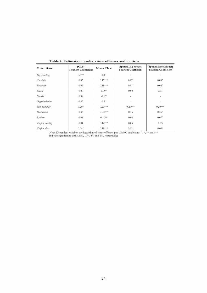
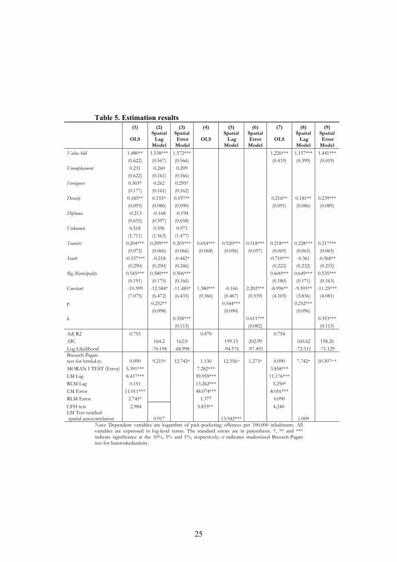
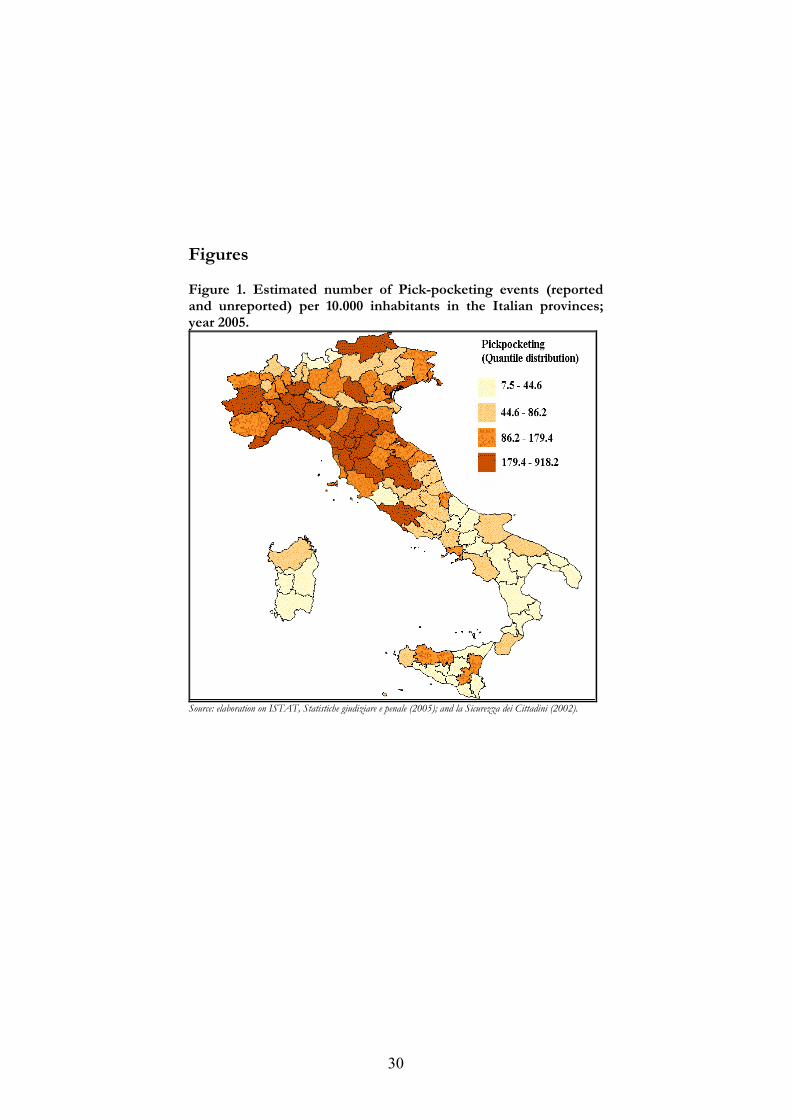
Table 4 compares the results of tourism coefficients among the crime offences under study. The first column displays the OLS coefficients. All coefficients are positive, but only one is statistically significant, although at 10% level. For all models with a significant Moran I test, both the spatial lag and spatial error model are estimated. As indicated in columns 3 and 4, pick-pocketing is the only type of crime that exhibits an evident tourism effect. As a consequence, from now on we focus only on this type of crime (see Figure 1 for a map of pick-pocketing in Italy). [FIGURE 1 HERE] The first column of Table 5 shows the results of the OLS estimation of model (5). All parameters have the expected signs, although Unemployment, Diploma and Unknown are not statistically significant. Value added, Tourists and Density are significant and positive. Therefore, a 1% increase in tourist arrivals leads to an increase of 0.2% in pick-pocketing. [TABLE 5 HERE] The adjusted R2 indicates a good overall fit (adj. R2 = 0.755). The diagnostic tests detect spatial autocorrelation (the Moran I test is high significant with a p-value of 5.895*10-4) and no heteroskedasticity (the Breusch-Pagan test is 0.09 with a p-value of 0.735). The performance of the heteroskedasticity test can be seriously affected by the presence of serial autocorrelation. As Anselin points out (1988), the serial autocorrelation in the residuals determines the upward bias of the test of heteroskedasticity, causing an over-rejection of the null hypothesis of

12

homoskedasticity. In our case, the Breusch-Pagan statistic test is sufficiently low and we do not need to implement a specific test for heteroskedasticity corrected for the presence of spatial autocorrelation. When the Moran I test is significant, the spatial econometric literature proposes the Langrage Multiplier (LM) test in order to find out which spatial model best fits the data. There are two variants of the LM test: the LM-lag and the LM-error test. The former tests the null hypothesis of no spatial autocorrelation in the dependent variable. The latter tests the null hypothesis of no significant spatial error autocorrelation. In our case, both tests can be rejected with extremely low probability of having incurred in type I error. Then, the Robust Langrage Multiplier (RLM) tests are performed. The RLM-error test corrects for the presence of local spatial lag dependence, assuming the absence of this kind of autocorrelation, i.e. the null hypothesis is λ = 0. Similarly, the RLM-lag statistic tests the null hypothesis that ρ is zero, correcting for the presence of local spatial error dependence. Both RLM statistic are distributed as χ2(1). The RLM lag and the RLM error statistics are respectively 0.15 (i.e. p-value = 0.697) and 2.74 (i.e. p-value = 0.097). In order to test the robustness of the spatial error model, the Common Factor Hypothesis test is performed (CFH). The CFH statistic yields 2.984; the corresponding p-value is 0.965. All results are coherent and show that the spatial error model performs better than the spatial lag model. The results of the spatial error model are presented in column (3) of Table 5. The λ coefficient is highly significant (value equal to 0.35). The Breusch-Pagan tests reported in the Table show that the problem of heteroskedasticity is not present either in the spatial lag model (p-value = 0.17) or the spatial error model (p-value = 0.19). As before, Value added, Tourists, South and Density are significant (spatial error model, column 3). The values of the spatial model coefficients are similar in magnitude to the ones of the OLS coefficients. Foreigners is weakly significant; a one percent increase in the share of foreigners would induce an increase in pick-pocketing of about 0.29%. Again, Tourists is positive and, on average, a 1% increase in tourist arrivals raises the level of pick-pocketing by 0.2% approximately. An increase in Density and Value added brings higher levels of street crime. The dummy variable South is negative: it catches the structural difference between the South and the rest of Italy. The descriptive analysis of pick-pocketing highlights how crime is a matter for which, on average, Central-Northern provinces

13

suffer the most (see again Figure 1). As expected, the dummy variable BigMun is positive as the big size cities experience a higher level of crime. Unemployment and Diploma variables are not significant, even if they have the expected signs. Those results are not a novelty in the economic literature on the determinants of crime in Italy (see, for an instance, Buonanno et al., 2009). From column 4 to column 9 two reduced form models are run in order to check the robustness of the estimates. In particular, in columns 7-8-9 the model is limited only to the significant variable of solutions (1) - (3). The tourism variable is still highly significant, along with the other variables and controls, and positive in both spatial models. 5.2 The geography of destinations and the social cost of tourism

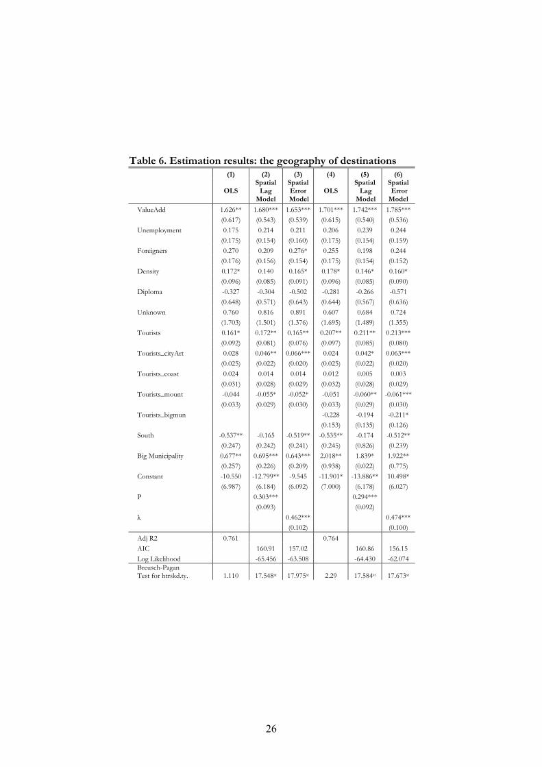
In order to control whether the geography of tourist destinations alters the impact of tourism on crime, we add three multiplicative dummies to the base model: Tourists_coast, Tourists_mount, and Tourists_cityart, the findings are presented in the first column of Table 6. The heteroskedasticity test is not significant and the p-value of the Moran I test is less than the one percent level. The two LM tests for spatial model are significant; in this case, RLM tests indicate that the spatial error model is the best, while the CFH test suggests the spatial lag model. However, the outputs of the two models are quite similar (see columns 2 and 3). Tourists_mount and Tourists_cityart are significant (although the former only at 10% level), while Tourists_coast is not. Notably, Tourists_mount and Tourists_cityart have an opposite impact on crime: the former is negative, while the latter is positive.

[TABLE 6 HERE]

In columns 4-6, a new interaction variable (Tourists_bigmun) is included to capture the tourism effect in big size towns. The diagnostic tests suggest considering the spatial error model as the most robust. Surprisingly, Tourists_bigmun is significant (at the 10% level) and negative. However, by summing the coefficients of Tourists_bigmun and Tourists, we find that the effect of tourism in provinces with big size cities is insignificant. Hence, the marginal effect of tourism on crime rate seems to decrease with the size of destinations: in overcrowded large cities the negative effect of tourism is almost negligible. In general, the results suggest that tourist presence generates a relatively lower impact on crime in mountain

14

destinations and a higher impact in art cities: a 1% increase in mountain tourism causes pick-pocketing offences to increase by 0.152% with respect to the other locations [= 0.213% + (-0.061%)]; the same variation in the arrivals determines an increase of offences by 0.276% in art city [= 0.213 + 0.063]. A possible explanation of these results might depend on the geographical characteristics of different destinations. Mountain locations tend to be set in isolated clusters and, except for few “hot” spots, tourists are scattered along the territory, but even in the “hot” spots, the specific type of clothes worn in the mountains may reduce the likelihood to be victims of pick-pocketing. Furthermore, the physical conformation of mountain locations makes the escape harder for offenders. On the contrary, art city destinations are characterised by high density of tourists and residents, and for several periods of the year they are overcrowded. As a consequence, the high concentration of tourists fosters opportunities for crime and, accordingly, higher crime rates. Surprisingly, we observe that the marginal effect of tourism on crime rate is decreasing with respect to the size of the cities; hence, in big cities no tourism effect is found on the pick-pocketing rate. We now turn to calculating the social costs of pick-pocketing linked to an increase of the presence of tourists. The starting point is a recent study of Detotto and Vannini (2010) in which the authors measure the social costs of crime offences for a sub-set of crime types in Italy for 2006. They find that the social costs exceed the Italian GDP by 2.6%. In the quoted work the social burden of pick-pocketing is calculated to be equal to € 124 million. Using the same estimates, we can calculate the marginal cost associated with an increase of pick-pocketing as a result of the rise of tourism arrivals: on average, at a national level, an increase in tourism arrivals by 1% should produce an increase in pick-pocketing in all provinces of 0.213%5 per year, which is equal to a social cost of 264,120 euros (4.47 euros per 1,000 inhabitants). In art city destinations the effect is higher by 0.063%, (an average marginal cost of € 5.80 per 1,000 inhabitants); while in mountain destination it is lower by 0.151% (an average marginal cost by € 3.17 per 1,000 inhabitants).

5 Here we are referring to tourism coefficient of the spatial error model.

15

5.3 A robustness check Finally, in order to check the robustness of the previous results, we

re-estimate the model (5) adding an interaction variable at a time. The results are presented in Table 7. Given the LRM tests and CFH tests, in all specifications the spatial error model is to be preferred. The λ coefficients are still positive and extremely significant. As before, Tourists_cityart is positive and highly significant at the 1% level (see column 3). Tourists_mount and Tourists_bigmun show a negative crime effect (in column 9 and 12, respectively), while Tourists_coast is not statistically different from zero (see column 6).

[TABLE 7 HERE]

An important issue to check is the exogeneity between tourism and crime rate. If tourism is not exogenous, we might expect that a shock in crime rate would impact tourism arrivals. In this case, our findings and the Langrage Multiplier tests for spatial error and lag dependence would be biased (Anselin, Varga and Acs, 2000; p. 506). In order to test the potential exogeneity of the tourism variable, the Durbin-Wu-Hausman test is used (Davidson and MacKinnon, 1993; pp. 237-242). In practice two OLS regressions are run. In the first regression, the variable suspected to be endogenous, namely tourism arrivals, is regressed on all exogenous variables and the instrument, and the residuals are retrieved; then in the second regression, the original (linear) model is re-estimated including the residuals from the first regression as additional regressors. Our goal is to identify an instrumental variable that is correlated with tourism variable but not with crime rate. Then, the following set of instrumental variables for tourism arrivals is considered: number of museums per province, proportion of the total sea area per province, and maximum altitude per province. Hence, the Durbin-Wu-Hausman test is implemented. In the first stage, the identifying instrumental variables perform reasonably well, while in the second step, the coefficient on the first stage residuals is not significantly different from zero6. This result indicates that we could not reject the null hypothesis of exogeneity of tourism variable.

6 The results of Durbin-Wu-Hausman procedure are available from the authors upon request.

16

6. Conclusions The presence of tourists fosters criminal activities, but not all types of crimes are affected in the same way. Like previous research on this topic, our findings suggest the existence of tourism effects on street crime, particularly, on pick-pocketing offences. More precise estimations have been obtained using spatial econometric tools. When we discriminate for the types of destination, we find that the impact of tourist arrivals on criminal activity is lower in mountain locations than in art cities. These results can be explained by geography: the different conformation of the territory may act as incentive or disincentive to commit crime, for instance, in mountain destinations the probability to escape is likely to be low while in cities is expected to be relatively higher. Further explanations are, for instance, the different “technology” of crime in different type of destinations, in art cities the concentration of “easier” locations for pick-pocketing is higher (buses, metro, etc) so that the “accumulated technology” of pick-pocketing industry might be higher as well. Probably, also the different types of clothing in mountain and in city may affect the likelihood to be the victim of pick-pocketing. In the final part of the work we calculate the social cost of tourism in terms of pick-pocketing. Of course, this measure is indicative of one type of negative externalities, in order to target proper policy interventions it is essential to measure also the cost of other negative externalities, along with the sources of positive externalities. Such cost-benefit analysis is a necessary step to implement sustainable regional policies. However, this was beyond the scope of this paper, where the novelty was rather to investigate whether and how the positive impact of tourism can be reduced by the cost of additional crimes that it generates.

17

References Aguilò, E., Riera, A., and Rossellò, J. (2005) “The short-term price effect

of a tourist tax through a dynamic demand model. the case of the balearic islands” Tourism Management, 26: 359-365.

Akis, S., Peristianis, N., and Warner, J. (1996) “Residents' Attitudes to Tourism Development: The Case of Cyprus” Tourism Management, 17: 481-494.

Anselin, L. (1988) Spatial econometrics: methods and models, Kluwer Academic Publishers, Dordrecht.

Anselin, L., Varga, A., and Acs, Z. (2000) “Geographical spillovers and university research: A spatial econometric perspective” Growth and Change, 31: 501-515.

Budowski, G. (1976) “Tourism and environmental conservation: Conflict, coexistence, or symbiosis?” Environmental Conservation, 3:27-31.

Balaguer, J., and Cantavella-Jordà, M. (2002), “Tourism as a long-run economic growth factor: the Spanish case” Applied Economics, 34: 877-884.

Buonanno, P., Montolio, D., and Vanin, P. (2009) “Does social capital reduce crime?” The Journal of Law and Economics, 52: 145-170.

Becker, G. (1968) “Crime and punishment: an economic approach” Journal of political Economy, 76: 169-217.

Bloom, J. (1996) “A South African perspective of the effects of crime and violence on the tourism industry”, in Pizam, A. and Mansfield, Y. (Eds), Tourism, Crime and International Security Issues, John Wiley & Sons Ltd, Chichester.

Brau, R., Lanza, A., and Pigliaru, F. (2007) “How fast are small tourism countries growing? Evidence from the data for 1980-2003”, Tourism Economics, 13: 603-613.

Cerina, F. (2007) “Tourism specialization and environmental sustainability in a dynamic economy” Tourism Economics, 13: 553-582.

Chao, C.C., Hazari, B. R., and Sgro, P. M. (2004) “Tourism, globalization, social externalities, and domestic welfare” Research in International Business and Finance, 18:141-149.

Cracolici, M.F., and Uberti, T.E. (2009) “Geographical distribution of crime in Italian provinces: a spatial econometric analysis” Jahrbuch für Regionalwissenschaft, 29: 1-28.

Crotts, J. (2003) “Theoretical perspectives on tourist criminal victimization” Journal of Tourism Studies, 14: 92-98.

18

Crouch, G.I. (1994) “The Study of International Tourism Demand” Journal of Travel Research, 32: 41-55.

Cushman, C. A., Field, B. C., Lass, D. A., and Stevens, T. H. (2004) “External costs from increased island visitation: Results from the southern thai islands” Tourism Economics, 10: 207-219.

Davidson, R., and MacKinnon J.G. (1993) Estimation and inference in econometrics. Oxford: University Press.

De Albuquerque, K., and McElroy J. (1999) “Tourism and Crime in the Caribbean” Annals of Tourism Research, 26: 968-984.

De Mello-Sampayo, F., and De Sousa-Vale, S. (2010) “Tourism and Growth in European Countries: An Application of Likelihood-Based Panel Cointegration” ISCTE, Lisbon University Institute, Working Paper - 05/10.

Detotto, C., and Pulina, M. (2009) “Does more crime mean fewer jobs? An ARDL model” Working Paper CRENoS, 2009/05: 1-25.

Detotto, C., and Vannini, M. (2010) “Counting the cost of crime in Italy” Working Paper CRENoS, 2010/13: 1-20.

Dritsakis, N. (2004) “Tourism as a long-run economic growth factor: an empirical investigation for Greece using causality analysis” Tourism Economics, 10: 305-316.

Dwyer, L., and Forsyth, P. (1993) “Assessing the Benefits and Costs of Inbound Tourism” Annals of Tourism Research, 20: 751-768.

Eugenio-Martin, J. (2004) “Tourism and economic growth in latin-american countries: A panel data approach” Fondazione Enrico Mattei, Nota di lavoro 26.2004.

Faulkner, H.W., and Tideswell, C. (1997) “A Framework for Monitoring Community Impacts of Tourism” Journal of Sustainable Tourism, 5: 3-28.

Figini, P., Castellani, M., and Vici, L. (2007) “Estimating Tourist Externalities on Residents: A Choice Modeling Approach to the Case of Rimini” Fondazione Enrico Mattei, Nota di lavoro 76.2007.

Fujii, E. T., and Mak J. (1980) “Tourism and Crime: Implications for Regional Development Policy” Regional Studies, 14: 27-36.

Gunduz, L., and Hatemi-J., A. (2005) “Is the tourism-led growth hypothesis valid for Turkey?” Applied Economics Letters, 12: 499-504.

Ivanov, S., and Webster, C. (2007) “Measuring the impact of tourism on economic growth” Tourism Economics, 13: 379-388.

19

Haralambopoulos, N., and Pizam, A. (1996) “Perceived Impacts of Tourism: The Case of Samos” Annals of Tourism Research, 23: 503-526.

Jud, D. G. (1975) “Tourism and Crime in Mexico” Social Sciences Quarterly, 56: 324-330.

Lanza A., and Pigliaru, F. (2000) “Why are tourism countries small and fast-growing?”, in: A. Fossati and G. Panella (eds), Tourism and Sustainable Economic Development, Dordrecht: Kluwer Academic Publisher, 57-69.

Levantis, T., and Gani, A. (2000) “Tourism demand and the nuisance of crime” International Journal of Social Economics, 27: 959-967.

Lindberg, K., and Johnson, R.L. (1997) “Modelling Resident Attitudes toward Tourism” Annals of Tourism Research, 24: 402-424.

Lindberg, K., Dellaert, B.G.C., and Rassing, C.R. (1999) “Resident trade-offs. A choice modelling approach” Annals of Tourism Research, 26: 554-69.

Liu, J. C., Sheldon, P. J., and Var, T. (1987) “Resident perception of the environmental impacts of tourism” Annals of Tourism Research, 14:17-37.

Katircioglu, S. T. (2009) “Tourism, trade, and growth: the case of Cyprus” Applied Economics, 41: 2741-2750.

Lee, C., and Chang, C. (2008) “Tourism development and economic growth: A closer look at Panels” Tourism Management, 29: 180-192.

Lin, V. L., and Loeb, P. (1977) “Tourism and crime in Mexico: Some comments” Social Science Quarterly, 58: 164-167.

Marselli, R., Vannini, M. (1997) “Estimating a crime equation in the presence of organized crime: evidence from Italy” International Review of Law and Economics, 17: 89-113.

Marselli, R., Vannini, M. (2000) “Quanto incide la disoccupazione sui tassi di criminalità?” Rivista di politica economica, Ottobre 2000: 273-299.

McPheters, L. R., and Stronge, W. B. (1974) “Crime as an Environmental Externality of Tourism: Florida” Land Economics, 50: 288-292.

Pizam, A. (1982) “Tourism and Crime: Is There a Relationship?” Journal of Travel Research, 20: 7-10.

Ryan, C. (1993) “Crime, Violence, Terrorism and Tourism” Tourism Management, 14: 173 - 183.

20

Savona, E., and Di Nicola, A. (1996) “Dynamics of migration and crime in Europe: new patterns of an old nexus” Working Paper Transcrime, 8: 1-34.

Schubert, S.F. (2009) “Coping with Externalities in Tourism - A Dynamic Optimal Taxation Approach” Competence Centre in Tourism Management and Tourism Economics (TOMTE), Free University of Bozen-Bolzano.

Sonmez, S.F., and Graefe A.R. (1998) “Determining future travel behavior from past travel experience and perceptions of risk and safety” Journal of Travel Research, 37: 171-177.

Soukiazis, E., and Proença, S. (2008) “Tourism as an alternative source of regional growth in Portugal: a panel data analysis at NUTS II and III levels” Portuguese Economic Journal, Springer, 7: 43-61.

Tobler, W.R. (1970) “A computer movie simulating urban growth in the Detroit region.” Economic Geography, 46: 234-240.

UNWTO (2009), Historical perspective of world tourism, UNWTO. Van Tran, X., and Bridges, F.S. (2009) “Tourism and Crime in European

Nations” e-Review of Tourism Research (eRTR), Vol. 7, No.3.

21

Tables Table 1. The propensity to report and NOT to report by type of robbery in the Italian for macro-areas. Year 2002.

Street crimes Thefts in dwelling

Pick-pocketing Bag-snatching Car thefts

PROPENSITY TO REPORT

North 53.6 61.0 54.7 61.0

Centre 58.4 67.0 56.4 63.5

South 67.8 61.6 57.4 55.2

PROPENSITY NOT TO REPORT

North 46.4 39.0 45.3 39.0

Centre 41.6 33.0 43.6 36.5

South 32.2 38.4 42.6 44.8 Source: our elaboration on data from ISTAT, La Sicurezza dei Cittadini, 2002.

22

Table 2. List of explanatory variables

Name Definition Type of variable Source

ValueAdded Value added per capita at a base prices - Year 2000 Economic ISTAT, Conti provinciali 1995-2003

Unemployment People looking for a job /labor force * 100 - Year 2001 Economic ISTAT, Sistema di Indicatori Territoriali

Foreigner Percentage of foreign people residing in the province- Year 2004 Demographic ISTAT, Atlante Statistico dei Comuni

Density Density of population per square kilometre - Year 2001 Demographic ISTAT, Atlante Statistico dei Comuni

Diploma People with Italian diploma per 10.000 inhabitants - Year 2001 Human Capital

ISTAT, Atlante Statistico dei Comuni

Unknown Ratio of incidents with unknown offenders over the total recorded per crime typology Year -2002

Deterrence ISTAT, Statistiche Giudiziare Penali

Tourists Tourists official arrivals per square kilometre (Tourists choosing official accommodations) - Year 2005

Tourism ISTAT, Statistiche del Turismo

Tourists_coast Tourist arrivals per square kilometre in coastal provinces with small-medium size cities (zero otherwise)

Tourism Elaborations on ISTAT, Statistiche del Turismo

Tourists_mount Tourist arrivals per square kilometre in mountain provinces with small-medium size cities (zero otherwise)

Tourism Elaborations on ISTAT, Statistiche del Turismo

Tourists_cityart Tourist arrivals per square kilometre in small- medium size art cities (zero otherwise)

Tourism Elaborations on ISTAT, Statistiche del Turismo

Tourists_bigmun Tourist arrivals per square kilometre in provinces with big municipalities (zero otherwise)

Tourism Elaborations on ISTAT, Statistiche del Turismo

South Dummy variable: 1 if the province is located in the South of Italy; zero otherwise.

Dummy

Bigmun Dummy variable: 1 if the province contains a big municipality (i.e. a town with more than 250,000 inhabitants); zero otherwise.

Dummy

Table 3A. Descriptive statistic of dependent variables

Name Mean Median SD Min Max

Pick-pocketing 251.91 156.74 294.74 11.50 1712.90

Bag-snatching 31.07 18.02 39.14 0 279.57

Car thefts 374.57 368.61 172.68 69.86 822.58

Extortion 9.02 7.86 4.91 2.50 26.81

Fraud 161.17 148.4 50.68 80.26 384.14

Murder 1.01 0.74 1.10 0 6.92

Organized crime 2.19 1.63 2.15 0 13.73

Prostitution 3.00 2.68 1.94 0 8.44

Robbery 44.68 30.93 51.61 8.32 407.76

Theft in dwelling 346.96 348.88 148.79 72.64 737.62

Theft in shop 103.42 101.10 47.31 19.21 258.78

23

Table 3B. Descriptive statistic of explanatory variables

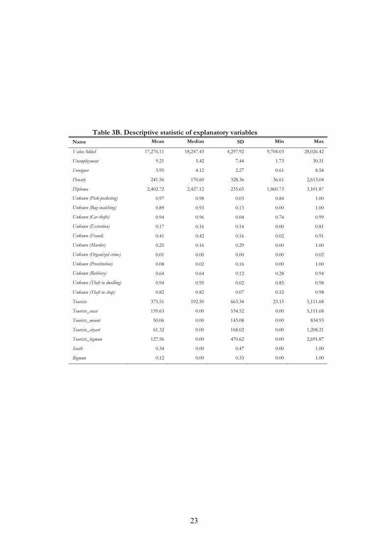
Name Mean Median SD Min Max

ValueAdded 17,276.11 18,247.43 4,297.92 9,704.03 28,026.42

Unemployment 9.21 5.42 7.44 1.73 30.31

Foreigner 3.95 4.12 2.27 0.61 8.58

Density 241.56 170.60 328.36 36.61 2,613.04

Diploma 2,402.72 2,427.12 235.65 1,860.73 3,101.87

Unkown (Pick-pocketing) 0.97 0.98 0.03 0.84 1.00

Unkown (Bag-snatching) 0.89 0.93 0.13 0.00 1.00

Unkown (Car thefts) 0.94 0.96 0.04 0.74 0.99

Unkown (Extortion) 0.17 0.16 0.14 0.00 0.81

Unkown (Fraud) 0.41 0.42 0.16 0.02 0.91

Unkown (Murder) 0.25 0.16 0.29 0.00 1.00

Unkown (Organized crime) 0.01 0.00 0.00 0.00 0.02

Unkown (Prostitution) 0.08 0.02 0.16 0.00 1.00

Unkown (Robbery) 0.64 0.64 0.12 0.28 0.94

Unkown (Theft in dwelling) 0.94 0.95 0.02 0.85 0.98

Unkown (Theft in shop) 0.82 0.82 0.07 0.52 0.98

Tourists 375.51 192.50 663.34 23.15 5,111.68

Tourists_coast 159.63 0.00 534.52 0.00 5,111.68

Tourists_mount 50.06 0.00 143.08 0.00 834.93

Tourists_cityart 61.32 0.00 168.02 0.00 1,208.21

Tourists_bigmun 127.56 0.00 470.62 0.00 2,691.87

South 0.34 0.00 0.47 0.00 1.00

Bigmun 0.12 0.00 0.33 0.00 1.00

24

Table 4. Estimation results: crime offenses and tourism

Crime offense (OLS) Tourism Coefficient Moran I Test (Spatial Lag Model)

Tourism Coefficient (Spatial Error Model) Tourism Coefficient

Bag-snatching 0.39^ -0.11 - -

Car thefts 0.05 0.17*** 0.06^ 0.06^

Extortion 0.06 0.18*** 0.00^ 0.06^

Fraud 0.00 0.09* 0.00 0.01

Murder 0.39 -0.07 - -

Organized crime 0.43 -0.11 - -

Pick-pocketing 0.20* 0.23*** 0.20*** 0.20***

Prostitution 0.36 -0.20** 0.35 0.35^

Robbery 0.04 0.10** 0.04 0.07^

Theft in dwelling 0.04 0.14*** 0.05 0.05

Theft in shop 0.06^ 0.19*** 0.06* 0.06*

Notes: Dependent variables are logarithm of crime offences per 100,000 inhabitants. ^, *, ** and *** indicate significance at the 20%, 10%, 5% and 1%, respectively;

25

Table 5. Estimation results (1) (2) (3) (4) (5) (6) (7) (8) (9)

OLS Spatial

Lag Model

Spatial Error Model

OLS Spatial Lag

Model

Spatial Error Model

OLS Spatial Lag

Model

Spatial Error Model

ValueAdd 1.480** 1.538*** 1.572*** 1.226*** 1.157*** 1.441*** (0.622) (0.567) (0.566) (0.419) (0.399) (0.419) Unemployment 0.231 0.260 0.209 (0.622) (0.161) (0.166) Foreigners 0.303* 0.262 0.295* (0.177) (0.161) (0.162) Density 0.185** 0.155* 0.197** 0.216** 0.181** 0.239*** (0.093) (0.086) (0.090) (0.091) (0.086) (0.089) Diploma -0.213 -0.168 -0.194 (0.655) (0.597) (0.658) Unknown 0.518 0.596 0.973 (1.711) (1.563) (1.477) Tourists 0.204*** 0.209*** 0.205*** 0.654*** 0.520*** 0.518*** 0.218*** 0.228*** 0.217*** (0.072) (0.066) (0.066) (0.068) (0.056) (0.057) (0.069) (0.065) (0.065) South -0.537*** -0.218 -0.442* -0.710*** -0.361 -0.568** (0.250) (0.250) (0.246) (0.222) (0.232) (0.233) Big Municipality 0.545*** 0.580*** 0.506*** 0.600*** 0.649*** 0.535*** (0.191) (0.175) (0.166) (0.180) (0.171) (0.163) Constant -10.399 -12.584* -11.485* 1.580*** -0.166 2.202*** -8.996** -9.595** -11.25*** (7.075) (6.472) (6.433) (0.366) (0.467) (0.339) (4.103) (3.836) (4.081) p 0.252** 0.544*** 0.252*** (0.098) (0.090) (0.096) λ 0.358*** 0.611*** 0.353*** (0.113) (0.082) (0.113)

Adj R2 0.755 0.470 0.754 AIC 164.2 162.0 199.15 202.99 160.62 158.26 Log Likelihood -70.198 -68.998 -94.576 -97.493 -72.311 -71.129 Breusch-Pagan test for htrskd.ty. 0.090 9.215st 12.742st 1.130 12.356st 1.273st 0.090 7.742st 10.307st * MORAN I TEST (Error) 5.391*** 7.282*** 3.858*** LM Lag 8.417*** 59.959*** 11.176*** RLM Lag 0.151 13.262*** 3.250* LM Error 11.011*** 48.074*** 8.016*** RLM Error 2.745* 1.377 0.090 CFH test 2.984 5.833** 4.240 LM Test residual spatial autocorrelation 0.917 13.542*** 1.009

Notes: Dependent variables are logarithm of pick-pocketing offences per 100,000 inhabitants. All variables are expressed in log-level terms. The standard errors are in parenthesis. *, ** and *** indicate significance at the 10%, 5% and 1%, respectively; st indicates studentized Breusch-Pagan test for heteroskedasticity.

26

Table 6. Estimation results: the geography of destinations (1) (2) (3) (4) (5) (6)

OLS Spatial

Lag Model

Spatial Error

Model OLS

Spatial Lag

Model

Spatial Error Model

ValueAdd 1.626** 1.680*** 1.653*** 1.701*** 1.742*** 1.785*** (0.617) (0.543) (0.539) (0.615) (0.540) (0.536) Unemployment 0.175 0.214 0.211 0.206 0.239 0.244 (0.175) (0.154) (0.160) (0.175) (0.154) (0.159) Foreigners 0.270 0.209 0.276* 0.255 0.198 0.244 (0.176) (0.156) (0.154) (0.175) (0.154) (0.152) Density 0.172* 0.140 0.165* 0.178* 0.146* 0.160* (0.096) (0.085) (0.091) (0.096) (0.085) (0.090) Diploma -0.327 -0.304 -0.502 -0.281 -0.266 -0.571 (0.648) (0.571) (0.643) (0.644) (0.567) (0.636) Unknown 0.760 0.816 0.891 0.607 0.684 0.724 (1.703) (1.501) (1.376) (1.695) (1.489) (1.355) Tourists 0.161* 0.172** 0.165** 0.207** 0.211** 0.213*** (0.092) (0.081) (0.076) (0.097) (0.085) (0.080) Tourists_cityArt 0.028 0.046** 0.066*** 0.024 0.042* 0.063*** (0.025) (0.022) (0.020) (0.025) (0.022) (0.020) Tourists_coast 0.024 0.014 0.014 0.012 0.005 0.003 (0.031) (0.028) (0.029) (0.032) (0.028) (0.029) Tourists_mount -0.044 -0.055* -0.052* -0.051 -0.060** -0.061*** (0.033) (0.029) (0.030) (0.033) (0.029) (0.030) Tourists_bigmun -0.228 -0.194 -0.211* (0.153) (0.135) (0.126) South -0.537** -0.165 -0.519** -0.535** -0.174 -0.512** (0.247) (0.242) (0.241) (0.245) (0.826) (0.239) Big Municipality 0.677** 0.695*** 0.643*** 2.018** 1.839* 1.922** (0.257) (0.226) (0.209) (0.938) (0.022) (0.775) Constant -10.550 -12.799** -9.545 -11.901* -13.886** 10.498* (6.987) (6.184) (6.092) (7.000) (6.178) (6.027) P 0.303*** 0.294*** (0.093) (0.092) λ 0.462*** 0.474*** (0.102) (0.100)

Adj R2 0.761 0.764 AIC 160.91 157.02 160.86 156.15 Log Likelihood -65.456 -63.508 -64.430 -62.074 Breusch-Pagan Test for htrskd.ty. 1.110 17.548st 17.975st 2.29 17.584st 17.673st

27

Table 6. ( cont inued)

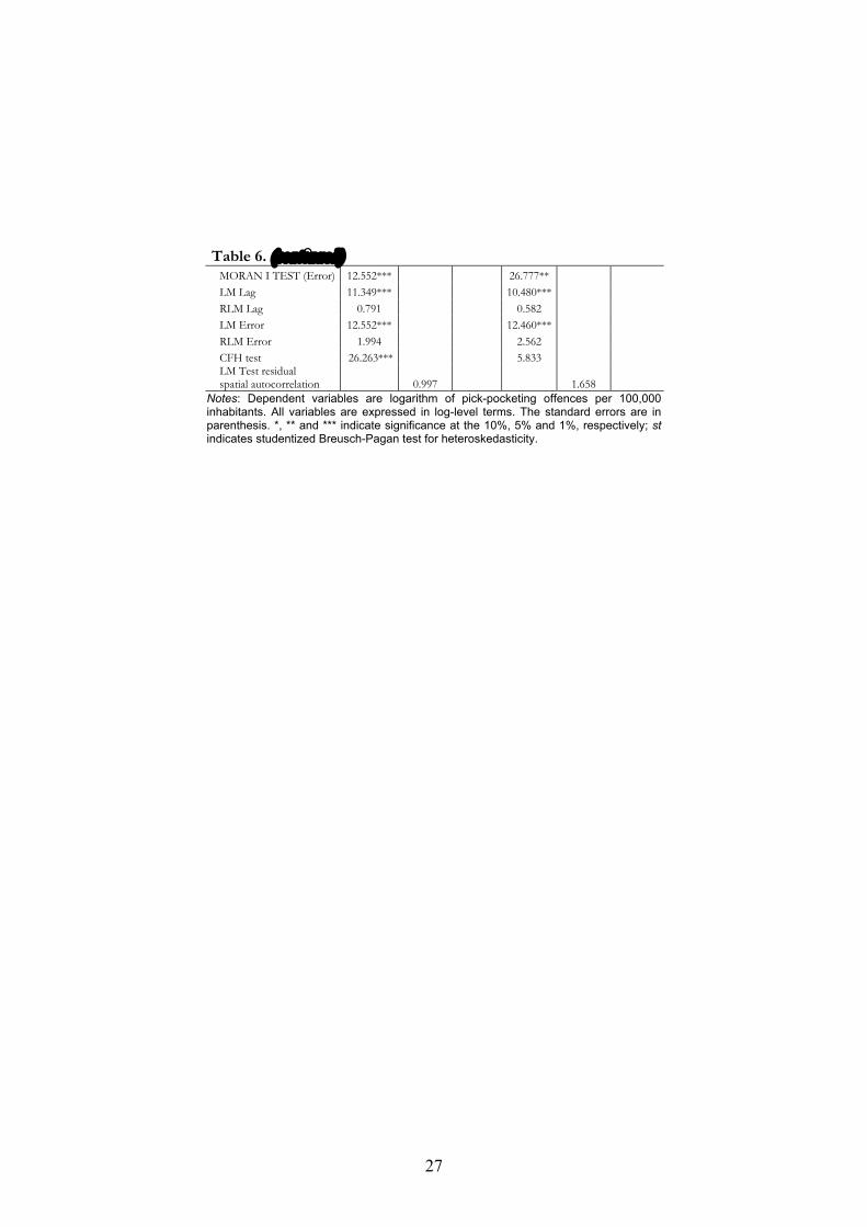
MORAN I TEST (Error) 12.552*** 26.777** LM Lag 11.349*** 10.480*** RLM Lag 0.791 0.582 LM Error 12.552*** 12.460*** RLM Error 1.994 2.562 CFH test 26.263*** 5.833 LM Test residual spatial autocorrelation 0.997 1.658

Notes: Dependent variables are logarithm of pick-pocketing offences per 100,000 inhabitants. All variables are expressed in log-level terms. The standard errors are in parenthesis. *, ** and *** indicate significance at the 10%, 5% and 1%, respectively; st indicates studentized Breusch-Pagan test for heteroskedasticity.

28

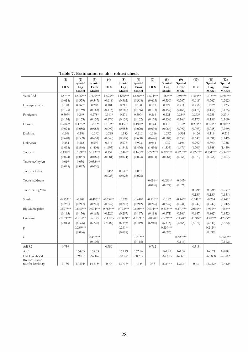
Table 7. Estimation results: robust check (1) (2) (3) (4) (5) (6) (7) (8) (9) (10) (11) (12)

OLS Spatial

Lag Model

Spatial Error Model

OLS Spatial

Lag Model

Spatial Error Model

OLS Spatial

Lag Model

Spatial Error Model

OLS Spatial

Lag Model

Spatial Error Model

ValueAdd 1.574** 1.506*** 1.476*** 1.593** 1.636*** 1.658*** 1.624*** 1.687*** 1.694*** 1.569** 1.615*** 1.696*** (0.618) (0.559) (0.547) (0.618) (0.562) (0.568) (0.615) (0.556) (0.567) (0.618) (0.562) (0.562) Unemployment 0.178 0.265* 0.202 0.181 0.215 0.190 0.193 0.222 0.211 0.256 0.282* 0.233 (0.175) (0.159) (0.163) (0.175) (0.160) (0.166) (0.173) (0.157) (0.164) (0.174) (0.159) (0.165) Foreigners 0.307* 0.249 0.278* 0.311* 0.271 0.309* 0.264 0.221 0.284* 0.293* 0.255 0.271* (0.174) (0.159) (0.157) (0.174) (0.159) (0.162) (0.174) (0.158) (0.160) (0.175) (0.159) (0.160) Density 0.204** 0.175** 0.221** 0.187** 0.159* 0.190** 0.144 0.113 0.152* 0.201** 0.171** 0.203** (0.094) (0.086) (0.088) (0.092) (0.085) (0.090) (0.094) (0.086) (0.092) (0.093) (0.085) (0.089) Diploma -0.249 -0.189 -0.292 -0.228 -0.183 -0.213 -0.316 -0.272 -0.324 -0.156 0.119 -0.215 (0.648) (0.589) (0.651) (0.648) (0.589) (0.650) (0.646) (0.584) (0.650) (0.649) (0.591) (0.649) Unknown 0.484 0.412 0.697 0.614 0.678 0.973 0.941 1.032 1.196 0.292 0.390 0.738 (1.698) (1.546) (1.408) (1.693) (1.542) (1.476) (1.696) (1.533) (1.476) (1.700) (1.548) (1.459) Tourists 0.190** 0.189*** 0.173*** 0.134 0.146** 0.163** 0.222*** 0.227*** 0.220*** 0.229*** 0.231*** 0.234*** (0.074) (0.067) (0.065) (0.081) (0.074) (0.074) (0.071) (0.064) (0.066) (0.073) (0.066) (0.067) Tourists_CityArt 0.019 0.036 0.053*** (0.025) (0.022) (0.020) Tourists_Coast 0.045* 0.040* 0.031 (0.025) (0.023) (0.025) Tourists_Mount -0.054** -0.056** -0.043* (0.026) (0.024) (0.026) Tourists_BigMun -0.221* -0.224* -0.233* (0.130) (0.130) (0.131) South -0.553** -0.202 -0.496** -0.534** -0.229 -0.448* -0.510** -0.182 -0.446* -0.541** -0.234 -0.443* (0.251) (0.247) (0.247) (0.247) (0.247) (0.242) (0.246) (0.247) (0.241) (0.247) (0.247) (0.242) Big Municipalità 0.577*** 0.645*** 0.604*** 0.763*** 0.773*** 0.640*** 0.504*** 0.538*** 0.470*** 2.096** 1.966** 1.958** (0.195) (0.176) (0.163) (0.226) (0.207) (0.197) (0.188) (0.171) (0.166) (0.947) (0.862) (0.832) Constant -10.71*** -12.31** -9.775 -11.073 -13.089** -11.995* -10.708 -12.96** -11.44* -11.960* -13.89** -12.73** (7.015) (6.396) (6.227) (7.007) (6.393) (6.419) (6.960) (6.315) (6.365) (7.070) (6.449) (6.372) p 0.289*** 0.241** 0.259*** 0.242** (0.096) (0.098) (0.096) (0.096) λ 0.457*** 0.331*** 0.328*** 0.364*** (0.102) (0.115) (0.116) (0.112) Adj R2 0.759 0.759 0.762 0.515 AIC 164.03 158.33 163.49 162.56 161.23 161.32 163.74 160.88 Log Likelihood -69.015 -66.167 -68.746 -68.279 -67.613 -67.661 -68.868 -67.442 Breusch-Pagan test for htrskd.ty. 1.130 13.594st 14.615st 0.70 13.718st 14.14st 0.43 16.24* st 1.273st 0.73 12.722st 12.442st

29

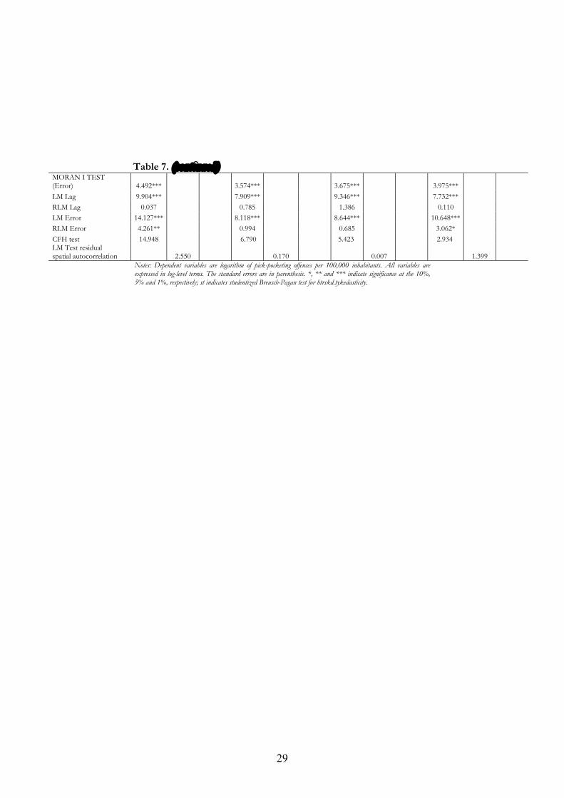
Table 7. ( cont inued) MORAN I TEST (Error) 4.492*** 3.574*** 3.675*** 3.975*** LM Lag 9.904*** 7.909*** 9.346*** 7.732*** RLM Lag 0.037 0.785 1.386 0.110 LM Error 14.127*** 8.118*** 8.644*** 10.648*** RLM Error 4.261** 0.994 0.685 3.062* CFH test 14.948 6.790 5.423 2.934 LM Test residual spatial autocorrelation 2.550 0.170 0.007 1.399

Notes: Dependent variables are logarithm of pick-pocketing offences per 100,000 inhabitants. All variables are expressed in log-level terms. The standard errors are in parenthesis. *, ** and *** indicate significance at the 10%, 5% and 1%, respectively; st indicates studentized Breusch-Pagan test for htrskd.tykedasticity.

30

Figures Figure 1. Estimated number of Pick-pocketing events (reported and unreported) per 10.000 inhabitants in the Italian provinces; year 2005.

Source: elaboration on ISTAT, Statistiche giudiziare e penale (2005); and la Sicurezza dei Cittadini (2002).

Ultimi Contributi di Ricerca CRENoS I Paper sono disponibili in: Uhttp://www.crenos.itU

10/14 Axel Gaut i e r , Dimi t r i Pao l in i , “Universa l serv ice f inanc ing in compet i t ive posta l markets : one s ize does not f i t a l l”

10/13 Claud io De to t t o , Mar co Vann in i , “Count ing the cost of cr ime in I ta ly”

10/12 Fabr iz i o Adr ian i , Luca G. De idda , “Compet i t ion and the s igna l ing ro le of pr ices”

10/11 Adr iana Di Lib e r t o “High sk i l l s , h igh growth: i s tour i sm an except ion?”

10/10 Vit t o r i o Pe l l i g ra , Andr ea I s on i , Robe r ta Fadda , I o s e t t o Doneddu , “Socia l Preferences and Perce ived Intent ions . An exper iment wi th Normal ly Deve loping and Aut is t ic Spectrum Disorders Subjects”

10/09 Luig i Gui s o , Lu i g i P i s ta f e r r i , Fab iano S ch i va rd i , “Credi t wi th in the f i rm”

10/08 Luca De idda , Bas sam Fat t ouh , “Rela t ionship Finance , Market F inance and Endogenous Bus iness Cyc les”

10/07 Alba Campus , Mar iano Por cu , “Recons ider ing the wel l -be ing : the Happy Planet Index and the i ssue of miss ing data”

10/06 Valen t ina Car ta , Mar iano Por cu , “Measures of wea l th and wel l -be ing . A compar ison between GDP and ISEW”

10/05 David For r e s t , Migu e l Ja ra , Dimi t r i Pao l in i , Juan d e Dio s Tena , “Inst i tut iona l Complex i ty and Manager ia l Eff ic iency : A Theoret ica l Model and an Empir ica l Appl ica t ion”

10/04 Manue la De idda , “Financ ia l Deve lopment and Se lect ion into Entrepreneursh ip : Evidence f rom I ta ly and US”

10/03 Giorg ia Casa l on e , Dan i e l a Sonedda , “Evaluat ing the Dis t r ibut iona l Effects of the I ta l i an F isca l Pol ic ies us ing Quant i le Regress ions”

10/02 Claud io De to t t o , Edoardo Otran to , “A Time Vary ing Parameter Approach to Analyze the Macroeconomic Consequences of Cr ime”

10/01 Manue la De idda , “Precaut ionary sav ing , f inanc ia l r i sk and port fo l io choice”

09/18 Manue la De idda , “Precaut ionary sav ings under l iqu id i ty constra ints : ev idence f rom Ita ly”

09/17 Edoardo Ot ran to , “Improving the Forecas t ing of Dynamic Condi t iona l Corre la t ion : a Vola t i l i ty Dependent Approach”

09/16 Emanue la Marro cu , Ra f fa e l e Pa c i , Mar co Pon t i s , “Intang ib le cap i ta l and f i rms product iv i ty”

09/15 Hel ena Marque s , Gabr i e l P ino , Juan d e Dio s Tena , “Regiona l inf la t ion dynamics us ing space- t ime models”

09/14 Ja ime Alvar ez , Dav id For r e s t , I smae l Sanz , Juan d e Dio s Tena , “Impact of Import ing Fore ign Ta lent on Performance Leve ls of Loca l Co-Workers”

09/13 Fab io Cer ina , Fran c e s c o Mureddu , “Is Agglomerat ion rea l ly good for Growth? Globa l Eff ic iency and Interreg iona l Equi ty”

09/12 Fede r i c o Crudu , “GMM, Genera l ized Empir ica l L ike l ihood, and Time Ser ies”

09/11 Franc e s ca Mame l i , Gera rdo Mar l e t t o , “Can nat iona l survey data be used to se lect a core se t of ind ica tors for moni tor ing the susta inabi l i ty of urban mobi l i ty pol ic ies?”

Finito di stampare nel mese di Agosto 2010 Presso studiografico&stampadigitale Copy Right

Via Torre Tonda 8 – Tel. 079.200395 – Fax 079.4360444 07100 Sassari

www.crenos.it