Tongji University Shanghai • Politecnico di Torino • Politecnico di Milano ‘’ POLITONG ‘’ Sino-Italian Double Degree Project Faculty of Information Technology Engineering Electronic Engineering Degree CRF POWERTRAIN TECHNOLOGIES METHODOLOGIES FOR THE ANALYSIS OF RELIABILITY OF ELECTRONIC DEVICES INTERNSHIP REPORT Student: Vinella Paolo Company Tutor: Ing. Massimo Abrate Academic Tutor: Prof. Alessio Carullo

Welcome message from author
This document is posted to help you gain knowledge. Please leave a comment to let me know what you think about it! Share it to your friends and learn new things together.
Transcript

Tongji University Shanghai • Politecnico di Torino • Politecnico di Milano
‘’ POLITONG ‘’ Sino-Italian Double Degree Project
Faculty of Information Technology Engineering
Electronic Engineering Degree
CRF
POWERTRAIN
TECHNOLOGIES
METHODOLOGIES FOR THE ANALYSIS OF
RELIABILITY OF ELECTRONIC DEVICES
INTERNSHIP REPORT
Student: Vinella Paolo
Company Tutor: Ing. Massimo Abrate
Academic Tutor: Prof. Alessio Carullo


Acknowledgements
First of all, I would like to thank the Politecnico di Torino for giving me the opportunity
to be engaged in a challenging degree course like Electronic Engineering. The unique
combination of such a skilling experience with an international double degree project
promoted by Politecnico di Torino, Politecnico di Milano and Tongji University of
Shanghai (China) like Politong, joint with the opportunity of an Internship in a valuable
Company like FIAT has enabled me to gain a set of effective engineering knowledge
mixed with an international challenging and wider academic context and a concrete
application into a state of the art Company environment.
An huge thank to Ing. Massimo Abrate, the Company tutor that has followed me during
the entire path of the internship with patience, responsibility, skilled suggestions and
polite willingness. Through him I have been able to be introduced toward the world of
R&D of FIAT Group, a comfortable and challenging environment.
Last but not the least, a thank must be addressed to my Academic tutor Professor
Alessio Carullo of Politecnico di Torino that has given me, with constant willingness and
through meetings, several inputs in terms of suggestions regarding the general
formulation and improvements concerning this report, and will have the forbearance to
read and evaluate it.


INDEX 1 Summary .......................................................................................................................................................................... 1
1.1 Introducing CRF FIAT Powertrain ............................................................................................................... 1
1.2 POLITONG Project ...................................................................................................................................... 1
1.3 Internship: brief introduction to the main goals ....................................................................................... 2
2 Introduction to the Analysis .......................................................................................................................................... 3
2.1 Electronic devices reliability in automotive field ....................................................................................... 3
2.2 Accelerated lifetime testing as measure of Reliability .............................................................................. 3
2.3 Life testing analysis: some Software solutions .......................................................................................... 4
2.4 From Product Prototype to Selling: Quality Requirements match .......................................................... 4
2.5 Mission Profile and product lifetime .......................................................................................................... 5
2.6 The “Intelligent Testing” approach ............................................................................................................ 5
2.7 Ingredients for an engineered Lifetime Analysis....................................................................................... 6
3 Theory Recalls .................................................................................................................................................................. 7
3.1 Distribution functions, Confidence and Confidence Interval ................................................................... 7
3.2 Contextualization ........................................................................................................................................ 8
3.3 Cumulative and Reliability (meaningful) functions .................................................................................... 8
4 Weibull model development ........................................................................................................................................ 9
4.1 Weibull distribution: main features ............................................................................................................ 9
4.2 Meaning of Scale Parameter .................................................................................................................. 9
4.3 Applied Stresses and : General Log-Linear Relationship ..................................................................... 10
4.4 Derivation of Weibull multi-stresses model equation ............................................................................ 12
4.5 Time-Varying Stresses .............................................................................................................................. 12
5 Maximum Likelihood Estimation (MLE) .................................................................................................................... 13
5.1 Easy case: Time-Independent Stresses .................................................................................................... 13
5.2 The realistic situation: Time-Varying Stresses ......................................................................................... 14
6 Fisher Matrix ................................................................................................................................................................... 16
6.1 Introduction to Fisher Matrix .................................................................................................................... 16
6.2 Expression of (local) Fisher Matrix terms ................................................................................................. 16
6.3 Variance estimation of -dependent distribution functions ................................. 17
7 Confidence boundaries ............................................................................................................................................... 18
7.1 The generic expression of confidence intervals ...................................................................................... 18
7.2 Confidence bounds for the Reliability function....................................................................................... 19
7.3 Confidence bounds for the Cumulative function ................................................................................... 20
7.4 Confidence bounds for the Failure Rate function................................................................................... 21
8 Other important estimated Parameters ................................................................................................................... 22

8.1 Shape Parameter and its boundaries ...................................................................................................... 22
8.2 Scale Parameter and its boundaries ........................................................................................................ 22
8.3 Life Time .................................................................................................................................................... 23
8.4 Reliability Value and its boundaries ......................................................................................................... 23
8.5 Mean Time To Failure (MTTF) .................................................................................................................. 23
9 FIAT LTA software environment ................................................................................................................................. 24
9.1 Introduction to FIAT LTA .......................................................................................................................... 24
9.2 Main ideas of the algorithm used in LTA for computation of confidence boundaries ........................ 25
9.2.1 Fisher Matrix computation ............................................................................................................... 25
9.2.2 Confidence Boundaries computation .............................................................................................. 26
9.3 Some examples of confidence boundaries computation: FIAT LTA vs Reliasoft ALTA........................ 27
9.3.1 FIRST TEST: 1 Profile with 2 ad-hoc built Stresses .......................................................................... 27
9.3.2 Second test: 1 Profile with 1 Stress taken from Weibull.com website ........................................... 34
9.3.3 Third test: 1 Profile with 2 Stresses with different shapes .............................................................. 36
9.4 Computation performance and limitations of confidence boundaries: previous method versus new
method .................................................................................................................................................................. 38
10 Conclusions .................................................................................................................................................................... 39
11 APPENDIX A – Developed source code for confidence boundaries.................................................................. 40
11.1 ComputeInverseLocalFisherMatrix function source code ...................................................................... 40
11.2 ComputeVarianceReliabilityAndFailureRate function source code ....................................................... 41
11.3 TVCalcolafitnessProfilo function source code ......................................................................................... 43
11.4 TVCalcolaStatisticheArray function source code .................................................................................... 45
11.5 WorkOutIntegralStep function source code ........................................................................................... 48
12 APPENDIX B - Derivation steps of each term of Fisher Matrix ............................................................................ 51
12.1 Computation of .......................................................................................................................... 51
12.2 Computation of ...................................................................................................................... 52
12.3 Computation of ........................................................................................................................ 52
12.4 Computation of ...................................................................................... 55
12.5 Computation of .................................................................................. 55
13 APPENDIX C – Computation steps of Reliability function derivatives ................................................................ 59
13.1 Derivative in respect to parameter ...................................................................................................... 59
13.2 Derivative in respect to each parameters .......................................................................................... 59
14 APPENDIX D - Computation steps of Failure Rate function derivatives ............................................................ 60
14.1 Derivative in respect to parameter ...................................................................................................... 60
14.2 Derivative in respect to each parameters .......................................................................................... 60
15 References ...................................................................................................................................................................... 62

Pag. 1
1 Summary
1.1 Introducing CRF FIAT Powertrain
Centro Ricerche Fiat (CRF for short), founded in 1978, has the mission to develop and transfer
innovative products, processes and methodologies through research and innovation in order to
improve the competitiveness of the products of the Fiat Group. Also through the cooperation with a
pan-European and increasingly global network of more than 1700 partners from Industry and
academia, CRF conducts collaborative research initiatives concerned with Sustainable Mobility,
targeting specifically the industrial exploitation of research. With a workforce of approximately 1000
full-time professionals, CRF develops research and innovation along the three principal axes:
Environmental Sustainability, Social Sustainability, Economically sustainable competitiveness.
The CRF research activities imply strategic competences not only in the field of automotive
engineering, but also in the fields of manufacturing, advanced materials, ICT and electronics, as well
as a wide range of state-of-the-art laboratories and extensive test facilities.
By December 2011, the Intellectual Property of CRF included 2860 patents both granted and
pending. Over recent years, the CRF has enabled the industrialization and commercialization of a
significant number of distinctive and highly innovative products for Fiat including, in the Powertrains
and vehicles area: Diesel Common Rail system (UNIJET and MultiJet); MULTIAIR and the new TwinAir
engine; energy saving air-conditioning systems, the Blue&Me connectivity product, Driving Advisor
and Magic Parking driver-assistance systems and the ECODrive eco-navigation solution.
CRF HQ in Orbassano (TO)
[Source: CRF website]
1.2 POLITONG Project
POLITONG Project is an international academic project issued by the Minister of Education of the
People's Republic of China and the Minister of Education, University and Research of the Republic of
Italy in Beijing, China on July 4th, 2005.
The two sides decided to develop a joint project in institutions of higher learning of the two
Countries. Tongji University from China and Politecnico di Milano and Politecnico di Torino from

Pag. 2
Italy developed a joint bachelor program in Engineering. Accordingly, the Sino-Italian Campus of
Tongji University was established.
The mission of POLITONG includes promotion of the development in higher education of China and
Italy; join training of internationalized talents familiar with the cultures of both Countries; enhance
the level of scientific R&D; support cooperation in education and industry of the two Countries.
Tongji University – Jiading Campus (Shanghai, China)
The training model is organized as follows:
First year in Italy: the first academic year entails basic courses taught in Italian.
Second year in Shanghai: Italian students attend the second year at Tongji University of
Shanghai with the Chinese students participating in the project. The courses are taught in
English by Italian lecturers from the two Italian universities and Chinese lecturers from Tongji.
Third year in Italy: having obtained 180 ECTS credits, also including a final project, Italian
students will obtain a joint Bachelor of Science degree (Laurea di primo livello) from
Politecnico di Torino and Politecnico di Milano.
Optional fourth year — 6 months in Shanghai: an additional 6-month period of study in
Shanghai is required in order to obtain a Chinese Bachelor of Science degree from Tongji
University. During this period students will primarily focus on research.
[Source: POLITONG website]
1.3 Internship: brief introduction to the main goals
The internship has been oriented in regard to the development of methodologies and software to
analyze the expectation of reliability of hardware devices. This process has required four stages:
analysis of the current techniques and development concerning those methodologies and software;
expansion with new methods including the design of optimized solutions; software development (on
National Instruments CVI environment) – that is, in order to bring the FIAT LTA software to its next
stage; validation testing based on real data.
The internship has been carried out in CRF headquarter in Orbassano, TO.

Pag. 3
2 Introduction to the Analysis
2.1 Electronic devices reliability in automotive field
The internship has been focused on electronic devices which are used in automotive application.
They are seen as “black boxes” samples – that is, they are not necessarily just “elementary parts” but
can also be complex circuit boards that may join more than one basic component on the same PCB.
A classic example is the microcontroller system for engine management. These devices are subject
to stress tests and, basing on test results under several kind of time-varying stresses and profiles, a
reliability analysis and model can be developed.
By developing a mathematical model based on probability theory, it is possible to obtain interesting
results concerning the reliability life expectation.
Inside a datasheet, a device is usually characterized by its producer with a reliability parameter that
is usually given in certain stress condition. The reliability information usually given by the producer of
the component regards a parameter in fixed stress condition (for example, the temperature range
for a diode).
We would like to develop a tool that allows to estimate the reliability also when stresses are different
from the nominal ones. Sometimes the producer does not give any kind of information regarding
this aspect.
Nowadays, about the 70% of vehicles a is based on electronics (both analog and digital) which starts
playing a more pressing role in the overall development of automotive products.
2.2 Accelerated lifetime testing as measure of Reliability
The goal of the analysis which follows this brief introduction is to find a mathematical and statistical
model, also translated as software, which is robust and representative enough to estimate the
reliability of electronic devices especially in terms of confidence boundaries. At the same time, it
should be taken into account the possibility to build a model which can fit on different scenarios and
be suitable in different applications.
The importance of producing reliable electronic systems is nowadays one of the main goals during
design stage. Reliability is a measure of “trustworthiness” that guarantees a specific device to
operate properly before the first failure occurs. A possible way to “compute” reliability passes
through the use of accelerated life time testing using a set of samples.
A well designed and tested hardware device allows it to work without failures for a known time
interval and let to reduce economic and time costs, as well as the producer will be able to establish
more realistic and optimized thresholds concerning warranty, maintenance through the product’s
lifetime, repair and stocks.

Pag. 4
Accelerated lifetime testing means testing a set of hardware sample devices under a series of
stresses which levels are much higher than those regarding its real use scenario. This allows to
obtain useful information in terms of expected lifetime and damages (that is, reliability) in an
“accelerated” way. Furthermore, the method allows to determine reliability boundaries after
developing a reliability statistical model that is also valid for real usage stresses scenario (“mission
profiles”).
A set of n samples is set under accelerated tests. Each sample is associated to one of m Profiles, with
n≥m, each of which is composed of several stresses (temperature, voltage,… and so on).
After acquiring experimental data from accelerated lifetime tests and choosing a suitable statistical
distribution as function of applied stresses, it is possible to develop a model that allows to compute
the characteristic parameters of the statistical distribution and, with further computation, determine
the confidence boundaries of those reliability functions.
In the following chapters each of those aspects will be covered, assuming that experimental data has
already been provided (that is, someone has already executed lifetime accelerated stresses for us).
After briefly recalling some concepts regarding the statistical model itself, a theoretical analysis
concerning a way to compute confidence boundaries has been devised and implemented as ANSI
C-like software to obtain charts of reliability functions as function of time completed with their
confidence boundaries.
2.3 Life testing analysis: some Software solutions
Reliasoft® currently offers a software called ALTA (Accelerated Life Testing Data Analysis Software
Tool), to carry out this kind of reliability analysis.
By the way, FIAT has recently set the goal of developing an own software, called LTA, which
provides similar functionality to ALTA in terms of reliability analysis.
At the moment, the product is almost complete but still does not include confidence intervals for the
reliability analysis in a time-varying stresses scenario: this is the final goal of this internship.
2.4 From Product Prototype to Selling: Quality Requirements match
The design of a product does not simply ends up with the check of meeting requirements. Every
time a product is designed, it must pass through two crucial phases:
STEP 1 : VALIDATION. It consists of a set of tests which are directly performed on the
designed prototype and are required to show possible malfunctions, in order to establish
whether the prototype requires or not further adjustments;
STEP 2 : QUALIFICATION. The product is now in its final stage and production engineering
tools help to make a final certification on it, in order to ensure a fully working device ready to
be put on the market. Usually certification is made by the Company itself, while in some

Pag. 5
scenarios, especially when standard protocol certifications are required to be complied, the
product sample might be checked from external Commissions/Consortiums too.
Even when present, European rules regarding products’ homologation are currently not so strict, but
final users’ requirements usually are. With a more and more pressing market competitors, the goal
of achieving better quality should become an aspect on which to focus much better than in past.
FIAT is currently working to improve the qualification and quality levels of its products, in order to
provide a global product quality that is much higher than both the standards set by homologation
and the ones that the final customer would like to see in a datasheet.
2.5 Mission Profile and product lifetime
The mission profile is a specific set of real stress cycles that are applied to a product during its entire
lifetime. For instance, a simple example of mission profile is the one that requires the use of the
product in a very cold environment for 10 years.
It would be nice for a Company to ensure that the expected lifetime of its product is strong enough
to match a particular mission profile that the customer would require for its application. Obviously it
is much better for the designer of the product to answer about the product lifetime if applied in
different scenarios and, thus, under more than one mission profile.
A statistic-mathematical model with a certain degree of complexity can be used to make a statistical
analysis regarding reliability of damage models of hardware devices: a software that implements
such kind of algorithms can be built to match this goal.
Usually a not enough complex model is developed to ensure test feasibilities under several scenarios
(that is, under several mission profiles). Current methodology used by several Companies is just able
to estimate the lifetime expectation under a particular mission profile but not for more than one.
2.6 The “Intelligent Testing” approach
A possible solution to the limits just illustrated is called robust validation, which can show the
margins on mission profiles. The so called “intelligent testing” methodology is used for this goal, and
it basically consists of let a sufficiently large number of sample devices reach their breaking (or
failure) point. A reliability model as function of mission profiles is thus developed - that is, what
actually happens to the component in terms of reliability while used during their lifetime.
At the moment, this approach also comes with disadvantages. The first one refers to the higher
degree of complexity in respect to the traditional ways of testing. Furthermore, a few people is
skilled and/or motivated to handle this topic. And, last but not the least, the costs of robust
validation are much higher than the traditional ways to perform tests.

Pag. 6
2.7 Ingredients for an engineered Lifetime Analysis
A complete lifetime analysis information, which should always be present inside the datasheet of any
hardware component must include:
Most probable value – the average (mean) expectation time;
Result confidence – an established percentage, over the total samples, that expresses the
degree of reliability of our range;
Confidence interval – it accompanies the most probable value by providing the range of
credible values for that parameter’s expectation.
As already stated, a mathematical model based on physics and statistic tools must be used.

Pag. 7
3 Theory Recalls
3.1 Distribution functions, Confidence and Confidence Interval
If one measures several times a particular quantitative characteristic of an object, under certain
conditions (such as a sufficiently large number of measures each of which is an independent event)
a Gaussian distribution will result. We will assume the Gaussian function as the starting point of our
analysis, to briefly introduce some concepts that will be used very frequently for our final goal.
The Normal (or Gaussian) probability density function is:
√
Equation
3.1-1
With the average value and the standard deviation (the square root of the variance ).
Let us recall some definitions that we have already briefly introduced so far. We will take into
account the Gaussian distribution. However, the same concepts can be applied without any change
in their intrinsic definition to other probability functions as well.
Confidence: is a fraction (expressed as percentage %) of the integral in the open domain ( , )
of the Gaussian distribution (which equals to 1, that is 100%). For example, a confidence degree of
95% means to consider the 95% of the area under the Gaussian function:
Confidence interval: the interval in which the measures fall in respect to the confidence previously
specified:
𝜇 𝜇 𝜎 𝜇 𝜎
𝜎
𝑓 𝑥
𝑥
0,95
CONFIDENCE INTERVAL

Pag. 8
It should be simple and immediate to guess that the standard deviation for the Gaussian distribution
is a particular value of confidence interval once a 68,26% confidence is set.
The complete expression of a measure (a reliability measure in our case) is thus:
AVG VALUE CONFIDENCE_INTERVAL @ CONFIDENCE OF [ ]% Equation
3.1-2
3.2 Contextualization
In the analysis that follows, the x-axis is the time axis and is denoted as t and measured in seconds
or its multiples. The y-axis represents instead the fraction of sample devices that reach that particular
time value before breaking. From now on, let us forget about x variable and replace it with t variable.
3.3 Cumulative and Reliability (meaningful) functions
It seems convenient to introduce right now the definition of two functions. Basing on a chosen
probability density function f (t), we define F (t) and R (t) as follows:
CUMULATIVE FUNCTION. It is expression of the
percentage of broken devices, for every considered
time value:
∫
Equation
3.3-1
RELIABILITY FUNCTION: the dual function of the
cumulative function, it represents the percentage of
devices that still survive until the considered time value:
∫
Equation
3.3-2
In our study we will consider as lower bound of the
integration interval not less than 0: in fact, it is
completely pointless to let the time assume negative
values. The time zero equals to the instant of time when
tests start to be performed on the samples.
𝒇 𝒕
𝑭 𝒕
𝑹 𝒕
𝒕
𝒕
𝒕
𝜇
𝜇
𝜇
5
5

Pag. 9
4 Weibull model development
4.1 Weibull distribution: main features
The probability density function that we take into account is the Weibull distribution, because it is
meaningful and suitable to represent reliability of components, both mechanical and electronic ones.
The analytic expression of Weibull distribution is:
(
)
(
)
Equation
4.1-1
With >0 shape parameter (expression of the slope of the function) and >0 scale parameter
(which meaning will be clear in a few paragraphs).
A generic plot of Weibull function:
The mean (or expected) value of Weibull distribution is:
(
) ∫
Equation
4.1-2
The standard deviation is instead:
√ (
) (
)
Equation
4.1-3
The Cumulative and Reliability functions, which play a major role in the analysis that follows, are:
∫
(
)
Equation
4.1-4
(
)
Equation
4.1-5
4.2 Meaning of Scale Parameter
The scale parameter represents, in an intuitive and qualitative way, the constant time, usually noted
with the letter . A recall of this concept can be found for example in microelectronic devices theory
(as “relaxation time”) or while studying a simple RC circuit (“charge/discharge time”). For the
cumulative and reliability functions of Weibull distribution the meaning is almost the same. The scale
𝒇 𝒕
𝒕

Pag. 10
parameter is, in fact, the bond of the dependence of Weibull distribution function on stress profiles
that are applied to the sample device. is measured in seconds.
4.3 Applied Stresses and : General Log-Linear Relationship
Let us take into account a generic stress s(x). It will be defined as a particular equation in the stress
variable x, but we will try to “manipulate” it in order to make it appear as an exponential function in
the following form:
Equation
4.3-1
The reason of expressing each stress equation into this form is given by the general log-linear
relationship (GLL) that is needed in order to link each stress expressed as exponential form to the
scale parameter of Weibull function.
Let each represent one of the n stresses applied, while coefficients are the model parameters
to determine. While introducing the expression that follows, it is useful to remind that “equation
manipulation” means variable/constants changes; these operations are themselves a function that
we call :
∑
Equation
4.3-2
.
TIME-VARYING STRESSES. The further steps ahead in our analysis regards considering stresses as
time-varying (T.V.) functions and their influence on the model under development. We have to work
on and applying it another function, that is ( ), which represents the complete form
of a stress expression, which becomes function of a stress variable (transformed to be suitable in the
GLL form), function in turn of time. From now on, we use this representation:
∑ ( )
Equation
4.3-3
At this point, the most common stresses are defined as follows:
𝒇 𝒕 𝜼
𝒕
𝜼 𝟓𝟎
𝜼 𝟏𝟎𝟎
𝜼 𝟐𝟎𝟎

Pag. 11
ARRHENIUS RELATIONSHIP. It shows the dependence on temperature:
( )
Equation
4.3-4
Where: R is the reaction speed ; T the temperature which is time t dependent ; the activation
energy ; k the Boltzmann constant ; A constant to be determined.
How to get the form required from the GLL relationship? First of all, we make an important
assumption: we assume that the component’s life is inversely proportional to the stress’ strength
R(T(t)); we can subsequently lead us back to the GLL relation (Equation 4.3-2):
( )
⇔
{
⁄
⁄
⁄
Equation
4.3-5
The same assumption can be applied to other kind of stresses. Some of them are reported in the
following paragraphs, and it is possible again to manipulate their equations in the useful way
requested by the GLL relationship.
The stresses’ equations show below are just listed as matter of example. Obviously, the concepts
shown so far can be also applied to other equations describing other kind of stresses.
EYRING RELATIONSHIP. It shows the dependence on humidity:
( )
Equation
4.3-6
Where: D is the deterioration ; H the humidity which is time t dependent ; A and B constants to be
determined.
IPL – INVERSE POWER LAW RELATIONSHIP. It shows the dependence on mechanical vibrations and
fluctuations of power supply voltage:
Equation
4.3-7
Where: V is the stress level ; K and n constants to be determined.
COFFIN-MANSON RELATIONSHIP. It is another way to express the IPL relation, where V replaces V
variable. This is a way to simplify the analysis of a time-varying stress test by using a model based on
a constant stress. The expression is given by:
Equation
4.3-8
Where: V is the cycle range; C and are constants to be determined.

Pag. 12
4.4 Derivation of Weibull multi-stresses model equation
The GLL model can be “injected” into Weibull function with a simple substitution. We start by
considering the simplest expression of (that is, time invariant – see Equation 4.3-2) and we mix it with
the Weibull Equation 4.1-1; the passages and the final result are both shown below:
{
∑
(
)
(
)
Equation
4.4-1
∑ ∑ ( )
Equation
4.4-2
The unknown variables to be determined, in order to define the model, are: .
4.5 Time-Varying Stresses
If the applied stresses are also time-varying, it is necessary to reformulate the Weibull equation f(t)
and, thus, F(t) and R(t) as well. The modification will take into account the fact that a sample can be
subjected to a sequence of several tests, each of which executed with different stress levels
(intensities) that varies according to the time.
From an analytical point of view, it is sufficient to replace the term
each time it appears in our
probability functions with the following integral function:
∫
∑
Equation
4.5-1
STRESS PARAMETER (for instance, the humidity)
after applying the substitution function
Effect of that particular stress on 𝜼

Pag. 13
5 Maximum Likelihood Estimation (MLE)
The Maximum Likelihood Estimation (MLE) is a method of estimating the parameters of a statistical
model. When applied to a data set (which, in our case, come from previously made stress tests) and
given a statistical model (the Weibull distribution), maximum likelihood estimation provides
estimates for the model's parameters . Once this function is set up, the mean
value of the parameters can be found by computing the absolute maximum
point of the function.
The likelihood function is made up of two parts. The first one refers to the Fe failures (that is, devices
under stress tests that result broken at a given time), while the second term indicates the amount of
samples still alive S. This is the reason why Weibull function and reliability function are taken into
account. Each sample device under test is extracted during the tests phase at a particular value of
time, that we assume to be different for each sample which can be either broken (and thus be one
of the terms of the first summation) or still alive:
∏ ( )
∏
Equation
4-1
We usually work on the logarithmic version of the MLE function (sometimes indicated as ). The
reason is due to the intrinsic exponential behavior of Weibull function and its reliability function:
taking the logarithmic version of both them is much easier for computation:
∑ ( )
∑
Equation
4-2
Both terms are nothing new. Let us try to make them appear in an explicit form, remembering the
definition of functions f and R , and treating two situations.
5.1 Easy case: Time-Independent Stresses
In this case, the expression of to take into account for Weibull and reliability functions’ equations is
the one shown in Equation 4.3-2.
We obtain the following results:
∑ ( )
∑
∑ [
(
)
(
)
]
∑ [ (
)
]
Pag. 14
∑{ [
(
)
] (
)
}
∑ (
)
∑{ [
∑
(
∑
)
] (
∑
)
}
∑ (
∑
)
Equation
5.1-1
It is important to highlight that is only function of the parameters . The
function does not depends on time; “i" is the index of the applied stresses that, for this first case, does
not depends on time too. Finally, and represent, for each sample, its extraction time.
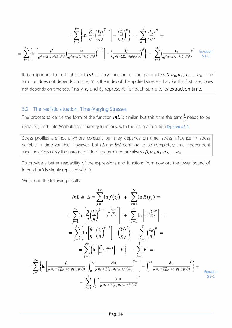
5.2 The realistic situation: Time-Varying Stresses
The process to derive the form of the function is similar, but this time the term
needs to be
replaced, both into Weibull and reliability functions, with the integral function Equation 4.5-1.
Stress profiles are not anymore constant but they depends on time: stress influence → stress
variable → time variable. However, both and continue to be completely time-independent
functions. Obviously the parameters to be determined are always .
To provide a better readability of the expressions and functions from now on, the lower bound of
integral t=0 is simply replaced with 0.
We obtain the following results:
∑ ( )
∑
∑ [
(
)
(
)
]
∑ [ (
)
]
∑{ [
(
)
] (
)
}
∑ (
)
∑{ [
] }
∑
∑{ [
∑
∫
∑
] ∫
∑
}
∑ ∫
∑
Equation
5.2-1

Pag. 15
The last expression of , Equation 5.2-1, is the one that we will take care of from now on. We have
finally derived an expression in the form:
Equation
5.2-2
Finally, through the application of a very specific genetic-like algorithm, the solution of the equation
can be found. This algorithm has already been previously devised by CRF, thus we already have a
solution, which a vector containing the mean value of its n+2 parameters:
{ } Equation
5.2-3

Pag. 16
6 Fisher Matrix
6.1 Introduction to Fisher Matrix
The Fisher matrix is part an important of the theory needed to provide helpful information related to
the mean and variance of a probability function; for example, the reliability function R(t).
Given the MLE function in its logarithmic form and its solutions { } ,
it is possible to build an (n+2) x (n+2) – size matrix based on second order derivatives (including
mixed ones) of function. The name of this structure is the Fisher matrix which is also known as
matrix. We will use the local version of the Fisher matrix, which is simpler to handle and more useful
for our analysis. It is defined as follows:
[
]
Equation
6.1-1
It can be shown that each of the parameters can be represented as a normal
distribution; the absolute maximum of the MLE function provides us their mean value. To compute
their standard deviation, one more step is needed, and the Fisher matrix is what we need.
In fact, the inverse matrix of is really meaningful because it contains the variance and the
covariance among the parameters and it can be interpreted as follow:
[
]
Equation
6.1-2
6.2 Expression of (local) Fisher Matrix terms
The derivatives of the logarithmic version of the Likelihood function in respect to each parameter
are the elements that, after a sign change, constitute the local Fisher matrix.
Each of their expressions need to be manually and analytically derived: while the final results are
shown below, all the single-step passages that drive to those results are stated in 12 APPENDIX B -
Derivation steps of each term of Fisher Matrix.

Pag. 17
∑{
}
∑
Equation
6.2-1
∑[ { } ∫
∑
]
∑[{ }∫
∑
]
Equation
6.2-2
∑[ ( )∫
∑
∫
∑
{ ( ) }∫
∑
]
∑ [ ∫
∑
∫
∑
∫
∑
]
Equation
6.2-3
6.3 Variance estimation of -dependent distribution functions
First of all, the terms which belong to the principal diagonal of matrix ( Equation 6.1-2 ) can be
used to characterize the standard deviation of each parameter: in fact, the Gaussian is now
complete, because we have all the required information: both the mean value and the standard
deviation (for example, for they are and √ .
The variance estimation of a generic function ( ) that depends on time
and parameters can be derived applying the following expression:
(
)
∑ (
)(
)
∑∑(
) (
) ( )
Equation
6.3-1
The variance is a time-dependent function: it means that, for each time value, a different variance
will accompany the function to which it relates. In fact, while the element taken from the inverse
local Fisher matrix are constant (that is, they express the variability of “fixed” real values: the
parameters), each derivative of the function in respect to each parameters is a time-dependent
function. Actually, all the expressions contain time-dependent integral functions.
Pag. 18
7 Confidence boundaries
The final goal of this entire analysis is to find the confidence boundaries of the functions that
depends on these parameters. A probabilistic function without boundaries is quite meaningless.
Boundaries should be seen as “delimiting borders” in worst case scenario.
The variance expresses itself a measure data dispersion and it represents the starting point to
compute the confidence interval (that is, boundaries), given a confidence degree which will be
noted hereafter with the real number .
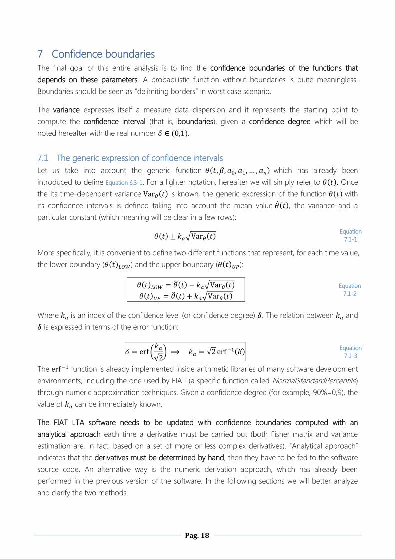
7.1 The generic expression of confidence intervals
Let us take into account the generic function which has already been
introduced to define Equation 6.3-1. For a lighter notation, hereafter we will simply refer to . Once
the its time-dependent variance is known, the generic expression of the function with
its confidence intervals is defined taking into account the mean value , the variance and a
particular constant (which meaning will be clear in a few rows):
√ Equation
7.1-1
More specifically, it is convenient to define two different functions that represent, for each time value,
the lower boundary ( ) and the upper boundary ( ):
√
√
Equation
7.1-2
Where is an index of the confidence level (or confidence degree) . The relation between and
is expressed in terms of the error function:
(
√ ) √
Equation
7.1-3
The function is already implemented inside arithmetic libraries of many software development
environments, including the one used by FIAT (a specific function called NormalStandardPercentile)
through numeric approximation techniques. Given a confidence degree (for example, 90%=0,9), the
value of can be immediately known.
The FIAT LTA software needs to be updated with confidence boundaries computed with an
analytical approach each time a derivative must be carried out (both Fisher matrix and variance
estimation are, in fact, based on a set of more or less complex derivatives). “Analytical approach”
indicates that the derivatives must be determined by hand, then they have to be fed to the software
source code. An alternative way is the numeric derivation approach, which has already been
performed in the previous version of the software. In the following sections we will better analyze
and clarify the two methods.

Pag. 19
Coming back to the main topic of this section, confidence boundaries must be computed for the
following functions:
Reliability Function R(t), which form for the Weibull distribution has already been stated in
Equation 3.3-2 ;
Cumulative Distribution Function F(t), defined in Equation 3.3-1 ;
Failure Rate Function FR(t), to be introduced and defined in the following sub-section 7.4
Confidence bounds for the Failure Rate function.
It is important to keep in mind that:
Each of those function depends both on time and on parameters (not only but also
which is, in turn, function of );
The variance of parameters-depending functions involves the use of the terms of the inverse
local Fisher Matrix, as clearly stated in Equation 6.3-1;
The function in respect to which to compute the variance must be derived in respect to the
parameters. Actually, as stated below, this task is much less complex (from a calculation point
of view) than the derivation of each term of the local Fisher matrix;
The final expression of the variance is time-varying and can be used, for each considered
time value, to determine the confidence boundaries for each value of the functions.
7.2 Confidence bounds for the Reliability function
The explicit form of the Reliability function is presented below, starting from Equation 4.1-5 and
keeping in mind that a time-variant (T.V.) stresses scenario (Equation 4.5-1) must be considered:
(
)
→
(∫
∑
)
Equation
7.2-1
From now on it is important to keep in mind what means (Equation 4.5-1) because it will be
frequently used instead of its explicit integral-function form for a more compact and lighter notation.
To determine the confidence boundaries one can simply consider and then compute
each derivative in respect to as stated in Equation 6.3-1, however this approach,
even if theoretically correct, is not the best one from the point of view of a software algorithm
implementation. Due to numeric approximation, in fact, the results that leads may result not
optimal. In other words:
The variance (that is, the confidence interval) can result more abundant than the real one;
Confidence boundaries may come with negative values – a physical nonsense.
The solution consists of an alternative method, which is more effective because it makes heavy
usage of the logarithm function mixed with its inverse function (the exponential), that will avoid
negative results.

Pag. 20
The starting point is the Reliability function written in another way, that is by applying in sequence a
function and its inverse one:
Equation
7.2-2
Now let us define a function u(t) as:
( ) ( ∫
∑
)
Equation
7.2-3
It is obvious to note that . At this point, the derivation of confidence boundaries
means finding those intervals for the u(t) function, that is:
√
√
Equation
7.2-4
Finally, the confidence boundaries for the Reliability Function can be found keeping in mind the
relation :
[ ]
[ √ ]
[ ] [ √ ]
Equation
7.2-5
The final step requires the explicit computation of the term that requires the derivatives of
u(t) in respect to each parameter. As done for the local Fisher matrix elements, the final expressions
are directly shown below, while single passages can be found in 13 APPENDIX C – Computation steps of
Reliability function derivatives.
Equation
7.2-6
∫
∑
Equation
7.2-7
7.3 Confidence bounds for the Cumulative function
The dual relationship that holds between the Reliability and the Cumulative functions (that is, they
are complementary and their sum, for each time value, is equal to 1 – see Equation 3.3-2) simplifies a
lot the computation of the confidence bounds for . In fact, for the boundaries this dual
relationship holds as well and it drives immediately to the final result:
Equation
7.3-1

Pag. 21
7.4 Confidence bounds for the Failure Rate function
As promised in the introduction of this section, we start by introducing the Failure Rate function:
given a particular distribution, it is defined as the ratio, for each time value, between the probability
density function f(t) and its Reliability function R(t):
Equation
7.4-1
Considering Weibull density and Reliability functions (Equation 4.1-1 and Equation 4.1-5), it can be derived
as follows keeping in mind the usual time-variant scenario:
(
)
(
)
(
)
⇒
∑
(∫
∑
)
Equation
7.4-2
The Failure Rate function expresses the units of failure for unit of time in respect to the ones that
survive (for example, “1 failure per month”).
The derivation of the confidence boundaries for the Failure Rate function can be done directly, using
the analytic approach without the use, in sequence, of the logarithm and exponential functions. This
means that we directly set and thus we work on FR(t) without any substitution, that
ends up with:
√
√
Equation
7.4-3
The same Equation 6.3-1 applies for the Failure Rate function as well, and again the final step requires
the explicit computation of the term that needs the derivatives of in respect to each
parameter. Once again, the final expressions of these derivatives are directly shown below, while the
single passages can be found in 14 APPENDIX D - Computation steps of Failure Rate function derivatives.
∑
Equation
7.4-4
∑
{ ∫
∑
} Equation
7.4-5

Pag. 22
8 Other important estimated Parameters
The estimation of confidence bounds for the Reliability, Cumulative and Failure Rate functions can
be completed with the computation of other parameters that strictly regard the estimation of those
functions. Some of them have already been presented in the previous paragraphs, some others will
be instead introduced as follow.
8.1 Shape Parameter and its boundaries
For the Weibull probability distribution, the shape parameter represents, with the scale parameter
, the way to identify a particular temporal evolution of the distribution itself. In fact, once and
are fixed, for each value of time it is possible to define the Weibull function.
So far we have considered the estimated value of , computed with the help of a genetic-like
algorithm. However, to be more precise, this value should be interpreted as the mean value for the
shape parameter: that is, .
Another look to the inverse of the local Fisher matrix (Equation 5.2-2) suggests that this matrix already
contains an important and useful piece of information to determine the confidence boundaries for
the shape parameter of Weibull distribution: in fact, we already have its variance, . If we recall
the Equation 7.1-2, we can immediately derive, for a given confidence degree, the confidence
boundaries for the shape parameter:
√
√
Equation
8.1-1
is obviously time-independent as well as its boundaries.
8.2 Scale Parameter and its boundaries
A similar analysis can be done for the scale parameter . Generically speaking, one gets:
√
√
Equation
8.2-1
However, for time-varying scenario, the scale parameter is also time-dependent because it is
expressed as an exponential linear combination of the applied stresses, which are time-varying (see
4.3 Applied Stresses and : General Log-Linear Relationship). It seems thus meaningless to compute both its
mean value and its confidence boundaries. In time-invariant situations, the scale parameter can
instead be computed as a single constant value, just like the shape parameter.
However, if from a purely mathematical point of view it is possible to derive the scale parameter and
its boundaries (for each time value!) applying the usual Equation 6.3-1. That means, once again, the

Pag. 23
inverse local Fisher matrix needs to be taken into account and the scale parameter must be derived
in respect to each parameter.
8.3 Life Time
The Life Time is defined as the time value to which corresponds a specific value of the failure
percentage. The failure percentage can be seen as one of the possible values of the y-axis of the
Cumulative function. To be more formal, for each time value, the Life Time can be seen as the
inverse function of the Cumulative function.
Even if from a purely mathematical point of view we have to think about an inverse function,
practice suggests a more direct approach to compute the Life Time value: once the failure
percentage is known, it is at first divided by 100. Once we get a value between 0 and 1, while the
Cumulative function is computed if , for a certain time value , this function is equal to the failure
percentage, then this temporal value is the Life Time we are looking for.
8.4 Reliability Value and its boundaries
Once the Life Time is known, it is possible to get immediately a reliability index of the devices under
test. Just to keep the same notation used in the previous paragraph, let be the Life Time. Thus,
the Reliability Value for this time value with its confidence boundaries is simply something we
already know very well: the Reliability function, of course. Since the function is known as well as its
boundaries:
Equation
8.4-1
8.5 Mean Time To Failure (MTTF)
The Mean Time To Failure is a synthetic estimation of the average (mean) time until a component
has its first failure. It can be seen as something related to the expected operating life before
something goes wrong and the device itself stops working properly.
For the Weibull distribution, the MTTF is defined as follows:
(
)
Equation
8.5-1
Where is the gamma function.
The MTTF depends on scale parameter: in this analysis we are always considering a time-varying
scenario, thus the same considerations already done for the scale parameter boundaries still hold: it
is not meaningful to compute to MTTF in this case because it depends on , which is in turn
function of the time and will make the Mean Time To Failure a function of time as well.
The Reliability function is instead an optimal estimation index for this purpose: in fact, it is convenient
to remember at this point that it indicated the probability that the device under test does not
encounter any failure until a predefined time value.
Pag. 24
9 FIAT LTA software environment
In the following section we will focus on FIAT LTA software. First of all we will briefly analyze its main
user interfaces and commands related to the analysis and implementation of the confidence
boundaries.
Then we will show some outputs that the software is able to provide once fed with input data (that is,
stress profiles and devices under test).
Finally, a comparison in terms of performance (computational time) between:
Confidence boundaries computation with the “old” method (numeric derivatives);
Confidence boundaries computation with this “new” method (the one developed in this
internship report).
We will see in the section 9.4 Computation performance and limitations of confidence boundaries: previous method
versus new method in what the main difference between those methods consists of.
9.1 Introduction to FIAT LTA
This paragraph contains a brief introduction to FIAT LTA software environment, with a brief recall of
the main functions that the tool is able to offer and which are strictly related to this report: Weibull
analysis in time-variant stresses scenario with confidence boundaries computation for Weibull
probability function and Reliability / Cumulative / Failure Rate functions.
Main interface and menu: through the software’s main interface it is possible to launch all its
subsections that will follow as next elements of this dotted list. First of all, it is possible both to
Pag. 25
Save Failure Table and Load Failure Table, a file with *.lta extension that contains everything
regarding the accelerated test: both inputs and the software’s outputs.
Failure Table: specifies, for each Sample under test, if it can be classified as Success or Failure
with its specific Time Value when this event happens. Furthermore, it is possible to associate
each failure with a specific Failure Code and its description, while on the other hand
components can be also defined with a Sample Code.
Profile Table (and Stress Profiles): allows to associate each sample with a specific (and single)
Stress Profile. Each Stress Profile is composed of several Stresses, each of which can be different
in terms of time evolution. However, the number of time-varying stresses for all the profiles is
fixed and always the same: for example, three different stress profiles can include voltage and
temperature stresses.
Profile Definition: the window through which the user can specify the time evolution of each
stress, defined as functions made of a set of joint segments.
Parameter Estimator: through the Genetic Algorithm, it is able to compute the maximum of the
Likelihood function and provide an estimation of the Parameters .
Statistical Analysis: the parameters previously estimated are finally fed as input of this section,
that is able to determine the plots of Weibull probability function and Reliability / Cumulative /
Failure Rate functions – now with confidence boundaries (the goal of this Internship itself!).
9.2 Main ideas of the algorithm used in LTA for computation of confidence boundaries
In the following paragraph the main ideas used to implement inside FIAT LTA the confidence
boundaries for Reliability function, Cumulative function and Failure Rate function will be discussed.
The entire analysis process starts once the user, after calculating with the genetic algorithm the
parameters , chooses the Statistical Analysis panel by clicking on Work Setting
Statistical Analysis Weibull and finally presses the button “Calculate”. Time-variant (T.V.) profiles
stresses have been previously entered inside LTA, thus the software already recognizes and knows
that a T.V. analysis must be performed in order to determine the confidence boundaries.
9.2.1 Fisher Matrix computation
First of all, it is necessary to calculate the local inverse Fisher matrix: in fact, it represents the starting
point for computing the variance of each function. We start by computing the local Fisher matrix;
finally a simple matrix inversion will provide its inverse form.
After zero-filling a matrix structure (n+2)x(n+2) big (where n is the number of active stresses that
constitutes each profile), for each element inside the matrix computation starts. We can observe that
not every element needs to be computed (about the 50% of the overall matrix): in fact, for example,
the second order mixed derivatives are equal.

Pag. 26
After an initial check that determines for each considered element if it really needs to be computed,
its value is actually calculated/updated gradually by scanning each profile.
For each profile, it is now necessary to consider all stresses and its associated samples. That is, it is
necessary to compute, according to the kind of element of the matrix (first row, principal diagonal or
upper triangular part) the its partial value due to the influence of the profiles and samples under test
currently considered.
If we look at each the analytical expression of elements of Fisher matrix, we will observe that their
structure is quite similar to the Likelihood function (they both have sums with the same indexes and
integral functions). This is why a template similar to the one already used to compute the lnL
function has been used.
In particular, each sample assigned to the profile currently considered is found and its event time
(failure or success) is recorded. All the required integral functions are thus computed from 0 up to
the currently considered time value. Obviously, not every integral function needs to be computed: it
depends on the specific element of the Fisher matrix we are considering. Once the integral functions
are computed, we analyze if the current event is a Success or a Failure and, according to its kind, we
can update one of the two sum terms exploiting the integral functions determined so far.
This process continues over and over again for each local Fisher matrix term that needs to be
computed. Once the process ends, the remaining terms inside the Fisher matrix (as stated before,
about the 50% of the total elements), previously not computed, are immediately determined:
1) Elements of the first column (except the first element) equals to the ones of the first row
(expect the first element);
2) Some elements in the upper triangular equal to the correspondent ones belonging to the
lower triangular.
Finally, it is necessary to change the sign of each element inside the Fisher matrix (in fact, it is
defined as a set of the NEGATIVE derivatives of the Likelihood function in respect to the parameters)
and compute its inverse form. The local inverse Fisher matrix is now ready to be used.
9.2.2 Confidence Boundaries computation
Once the inverse local Fisher matrix is determined, confidence boundaries need to be computed as
well. Obviously, for each considered function parameters-dependent, everything relies on the
computation of the variance. We recall, as already stated several times in the previous sections, that
the variance is time-dependent: for each time value of both Reliability and Cumulative and Failure
Rate functions, the variance needs to be computed. While LTA computes the value of those
functions for each time value, it is possible to carry out, in the meantime, the computation of the
variance for that particular time value and, thus, its boundaries.
For each function, each time the variance needs to be computed it is necessary to determine the
derivative of that function in respect to each parameter. Because they all depend, in turn, on integral

Pag. 27
functions, it is necessary for each applied stress to compute each integral function until the
considered time value (starting from the origin t=0, of course). The integrals are finally used and
mixed all together in order to compute the derivatives, which are in turn all considered with the
Fisher matrix elements in order to finally compute the numeric value of the variance.
The procedure needs to be applied for each function (thus, Reliability and Failure Rate functions –
we have seen before that boundaries for the Cumulative functions can be immediately derived from
the Reliability one).
The variance, together with the user-desired inputted index of confidence level, are finally combined
with the value of the function for each time value in order to derive the value of the upper and
lower boundary of that function for that specific value of time.
9.3 Some examples of confidence boundaries computation: FIAT LTA vs Reliasoft ALTA
In order to validate the written code for confidence boundaries, several tests have been used as
input to the FIAT LTA software. The aim of this subsection is to show the obtained results for three
among the most relevant validation tests, with a very brief illustration of what they consist of and
comparing these results with the ones provided by Reliasoft ALTA suite.
Both software can be tested in terms of provided output by feeding them with a set of predefined
inputs.
9.3.1 FIRST TEST: 1 Profile with 2 ad-hoc built Stresses
The first test is quite “special”, because it includes a set of inputs that have been computed by hand
following a specific procedure starting from a generic Weibull distribution.
We start with a Weibull function with fixed values for and . For example, we choose and
. We also assume a “time window” from 0 to 1000 hours.
After defining the distribution function, we identify the time values in respect to which the
cumulative area under the curve (in other words, the Cumulative function) reaches values 0.25 (25%),
0.50 (50%) and 0.75 (75). We call these values , and .
We assume to apply to some samples under test two stresses, and (for example voltage and
temperature stresses) that evolve as step functions with discontinuities at , and .
Furthermore, stresses have predefined magnitude values (that is, “stress levels”) multiplied by known
multiplying factors, marked on the stress curves in the following picture.
We choose 1, 1.2 and 1.5 as multiplying factors and magnitude values of 10V and 15V (for the
voltage profile), 300K and 360K (for the temperature profile).

Pag. 28
The influence of those stresses on the Weibull function will be an increasing of the cumulative areas,
each of which will be multiplied by the product, for each time interval, of the stresses’ multiplying
factors. After these new percentages are known, we normalize them such that their sum is 100%.
Let now be the number of total samples under test; we choose . These “new” percentages
just obtained will express how many sample, over their total amount, will reach their breaking point
(at time ) inside each time interval. We choose the breaking times for each sample in a very
specific way: we place the samples such that their failure times are x-values (horizontal coordinates)
of y-values (vertical coordinates) of the Weibull function more present in the neighborhood of which
the function has a greater slope, and less present everywhere else.
Now that each has been determined, we choose a subset of m samples, with , that
represents the number of samples that we decide not to make them fail: that is, still alive. We
assume in our case , one for each subset. We finally modify for those still surviving samples,
such that their new is smaller than the previous one (in fact, a success happens before a failure
time!).
This entire procedure is only apparently tangled: the scheme reported in the next page should
clarify the entire process required to develop this set of input to be fed into ALTA and LTA.
Matlab has been used to obtain Weibull distribution (and its cumulative function) by mean of the
following very simple script:
However, for a better clarity, those plots have not directly used inside this report - they have been
utilized in order to realize the following ones which use a richer formatting both for text and
graphics.
On the left side of the following charts, a brief explanation recalls the passages that have just
reported so far in order to build the final set of input data for FIAT LTA and Reliasoft® ALTA.
figure(1); hold on; grid on;
t = [0 : .1 : 1000];
wbl_pdf = wblpdf(t,700,4);
plot(t,wbl_pdf,'b');
title('Weibull f(t) - b=4 ; n=700');
figure(2); hold on; grid on;
wbl_cdf = wblcdf(t,700,4);
plot(t,wbl_cdf,'r');
title('Weibull F(t) - b=4 ; n=700');

Pag. 29
1
0.8
0.6
0.4
0.2
200 400 600 800 1000
2.5x10⁻³
2x10⁻³
1.5x10⁻³
1x10⁻³
0.5x10⁻³
200 400 600 800 1000
𝐭𝟐𝟓 ≅ 𝟓𝟏𝟑 𝐭𝟕𝟓 ≅ 𝟔𝟑𝟗
2.5x10⁻³
2x10⁻³
1.5x10⁻³
1x10⁻³
0.5x10⁻³
200 400 600 800 1000
1
1.5 1.5
1
1 1
1.2 1.2
𝐭𝟓𝟎 ≅ 𝟔𝟑𝟗
𝒕
𝒕
𝒕
𝒕
𝒕
𝒕
𝒇 𝒕
𝑭 𝒕
𝑺𝒕𝒓𝒆𝒔𝒔𝟏
𝑺𝒕𝒓𝒆𝒔𝒔𝟐
The Weibull distribution
plot f(t) for =4 and
=700.
The associated
cumulative function F(t),
useful to determine time
values when the
cumulative integral of
f (t) reaches 0.25, 0.5
and 0.75 values.
The time x-axis; t25% ,
t50% and t75% are now
known.
Two stresses are
applied: we assume
Stress1 as voltage…
…and Stress2 as
temperature.
The influence of the
stresses over the
Weibull distribution. The
plot f’(t) is qualitative,
but percentages are
computed. For example,
for the second sector:
25% * 1,5*1 = 37,5%
𝒇′ 𝒕
total:137,5%

Pag. 30
The latter percentages are normalized in respect to 100% (that is, a scaling down is made in respect
to the previous grand total equal to 137,5%). We thus obtain:
FIRST SECTOR (range to ): 25% 18,18%
SECOND SECTOR (range to ): 37,5% 27,27%
THIRD SECTOR (range to ): 45% 32,73%
FOURTH SECTOR (range to ): 30% 21,82%
Having previously assumed the total number of samples is equal to , we can relate the
previous normalized percentages to the number of samples for each sector:
FIRST SECTOR (range to ): 4 SAMPLES
SECOND SECTOR (range to ): 6 SAMPLES
THIRD SECTOR (range to ): 6 SAMPLES
FOURTH SECTOR (range to ): 4 SAMPLES
Finally, we have to pick up some values, each of which will be related to a device under test. If it
refers to a failure (Fe) no further adjustment needs to be done, while every time a success (S) is
considered (that is, we “transform” a failure into success), a “still alive” time must be taken into
account (less than the failure time previously assumed):
Everything is ready: both failure/surviving times have been determined, as well as stress profiles. We
can move on by feeding those inputs in both ALTA and LTA and see what they output.
Fe
Fe
Fe
Fe
Fe
Fe
S
Fe
Fe
S
S
Fe Fe Fe
Fe Fe
Fe
S
Fe
Fe
2.5x10⁻³
2x10⁻³
1.5x10⁻³
1x10⁻³
0.5x10⁻³
200 400 600 800 1000
𝒕
𝒇 𝒕
𝒕𝟐𝟓 𝒕𝟓𝟎
𝒕𝟕𝟓
t1=300
t2=380
t3=430
t4=484
t5=530
t6=545 t7=560
t8=575 t9=595
t10=625 t11=655 t12=686
t13=705 t14=718
5 t15=735
t16=748
t17=792
t18=816
t19=850
t20=900
t3=420
t8=568
t15=730
t19=840
Pag. 31
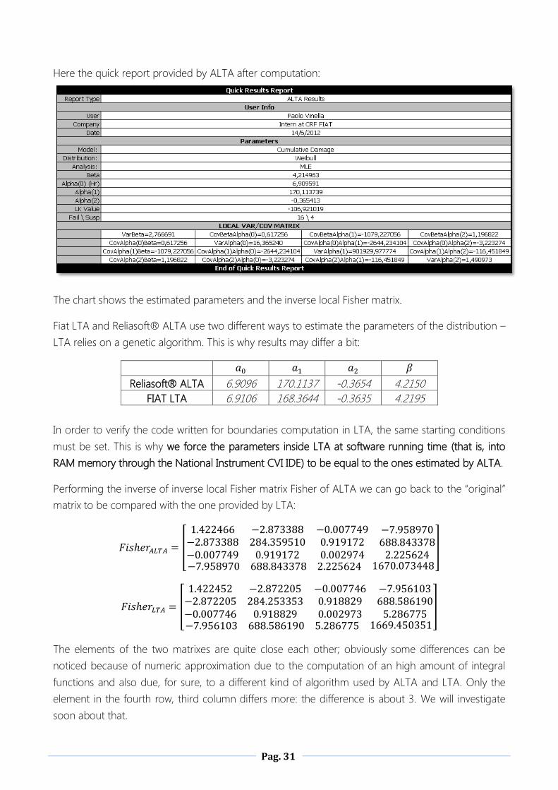
Here the quick report provided by ALTA after computation:
The chart shows the estimated parameters and the inverse local Fisher matrix.
Fiat LTA and Reliasoft® ALTA use two different ways to estimate the parameters of the distribution –
LTA relies on a genetic algorithm. This is why results may differ a bit:
Reliasoft® ALTA 6.9096 170.1137 -0.3654 4.2150
FIAT LTA 6.9106 168.3644 -0.3635 4.2195
In order to verify the code written for boundaries computation in LTA, the same starting conditions
must be set. This is why we force the parameters inside LTA at software running time (that is, into
RAM memory through the National Instrument CVI IDE) to be equal to the ones estimated by ALTA.
Performing the inverse of inverse local Fisher matrix Fisher of ALTA we can go back to the “original”
matrix to be compared with the one provided by LTA:
[
5 5
5 5
5 5
]
[
5 5 5 5 5
5 5 5 5
5 5 5 5 5 5
]
The elements of the two matrixes are quite close each other; obviously some differences can be
noticed because of numeric approximation due to the computation of an high amount of integral
functions and also due, for sure, to a different kind of algorithm used by ALTA and LTA. Only the
element in the fourth row, third column differs more: the difference is about 3. We will investigate
soon about that.

Pag. 32
The following are the plots of Weibull, Cumulative, Reliability and Failure Rate functions by ALTA:

Pag. 33
This is instead the output of the statistical analysis carried out by FIAT LTA. The red functions plots
are essentially, from a purely visual point of view, what the internship’s goal consists of.
Looking at the shapes and the values of the corresponding function plots in ALTA and LTA
(especially regarding the confidence boundaries, the red curves) it is possible to observe that they
essentially match.
So what about the difference of one element inside the Fisher matrix? I wanted to go deeper and try
to discover what the answer is or, at least, could be. At the beginning, I assumed that Fiat LTA had a
bug in computing correctly every element of the matrix: I tried to brutally overwrite in memory the
element that differs the most (5 5) with the one proposed and computed by ALTA ( 5 ).
The result on output function plots was immediate: Fiat LTA plots were not anymore correct, they
differed a lot in terms of confidence boundaries!
One can conclude that Reliasoft ALTA, when applied stresses are more than one, computes that
matrix element with applying a slightly different formula, and then a slightly different formula for the
variance (Equation 6.3-1) as well. In brief, both software they ensure almost the same matching output
results for boundaries computation, but after each software goes through some slightly different
intermediate steps and computations.
Two more tests will follow. This time a more synthetic output report will accompany them.

Pag. 34
9.3.2 Second test: 1 Profile with 1 Stress taken from Weibull.com website
The website Weibull.com has been extensively used to explore and expand some theoretical aspects
regarding Weibull distribution analysis in time variant scenario. Furthermore, it includes some
examples that can be used as inputs to fed Reliasoft® Alta. We now consider one of those and, as
already done in the previous test, we feed these inputs to both ALTA and LTA and we analyze the
outputs in terms of Fisher matrixes and boundaries plots.
The input set is made of 11 samples under test, all classified as Failures. They are all associated to a
single Profile made of one stress. The stress is an applied voltage that continually increases as multi-
step function over time, ranging from 2V to 7V.
We start again with the quick report provided by ALTA after computation:
Again, we compare the parameters computed by ALTA and LTA.
Reliasoft® ALTA 9.8421 -3.9985 2.6783
FIAT LTA 9.8442 -4.0006 2.6750
Once again, to verify the code written for boundaries computation in LTA, the same starting
conditions must be set - we force the parameters inside LTA at software running time to be equal to
the ones estimated by ALTA.
Performing the inverse of inverse local Fisher matrix Fisher of ALTA we can go back to the “original”
matrix to be compared with the one provided by LTA:
[
5 5 5
]
[ 5
5 55 5 5 55
]
The matrixes are very close each other.

Pag. 35
The following are the plots of Weibull, Cumulative, Reliability and Failure Rate functions by ALTA:

Pag. 36
This is instead the output of the statistical analysis carried out by FIAT LTA:
The output functions comes with boundaries which are estimated almost in the same way both from
Reliasoft® ALTA and FIAT LTA.
9.3.3 Third test: 1 Profile with 2 Stresses with different shapes
The input set is made of 6 samples under test, all classified as Failures. They are all associated to a
single Profile made of two stress. The first stress is an applied voltage that varies over time as a
triangular function with values between 4.5V and 5.5V, while the second stress represents an
increase of temperature over time as multi-step function in an overall range between 273K and
320K.
This time, Reliasoft® ALTA is not capable to carry out the statistical analysis: a pop-up window
informs the user that: <<An error occurred while conducting calculations. Unable to find an accurate
solution. Select another model or distribution and recalculate>>.
FIAT LTA is instead able to perform calculations and output both a set of estimated parameters and
statistical functions with their confidence boundaries. In particular:
Reliasoft® ALTA N/A N/A N/A N/A
FIAT LTA 13.1260 11.2494 -4.6391 32.2174

Pag. 37
FIAT LTA has computed the following local Fisher matrix:
[
5 5 5 5 5 5 5 5 5 5
5 5
5 5 5 5 5
]
Finally, this is instead the output of the statistical analysis carried out by FIAT LTA:
This third example is to show that both ALTA and LTA sometimes may both fail during parameters
estimation and/or during confidence boundaries computation, as well as it may happen, sometimes,
that due to numeric approximation the variance for some points of the Reliability / Failure Rate
functions becomes negative. This is meaningless, thus a pop-up window will inform the user that he
might want to execute again the genetic algorithm, change the confidence level, choose another
integration method or increase the number of integration steps in order to put the software in
better conditions to avoid errors, or at least reduce them in a smaller time-domain subset.
Finally, we take into account the Reliability function plot of this example to give an interpretation of
the results that those plots can provide. Once a selected stress profile is applied, at a confidence
level of 90%, we set a failure percentage of 20%. The software is able to tell us that 80% of samples
will be still alive (that is, 20% dead) after 270 hours of running time. However, in the worst case, they
will fail after 245 hours, while in the best case the amount of time before failure reaches 280 hours.

Pag. 38
9.4 Computation performance and limitations of confidence boundaries: previous
method versus new method
As already stated several times, the final goal of the Internship regards, after analyzing the
theoretical aspects behind the robust validation through accelerated life-time tests, the derivation of
confidence boundaries for the statistical analysis. We have previously seen how this can be carried
out: through the use of the inverse local Fisher matrix and the application of the equation that allows
to compute the variance of a generic function that depends on the parameters .
The previous version of LTA software (what we have previously defined as “old version”) was already
capable of computing the confidence boundaries, but the entire procedure made use of numeric
derivatives each time a derivate needs to be computed (thus, to determine the Fisher matrix and the
variance).
This internship makes LTA software possible to reach a new stage (“new version”): the difference in
respect to the previous methodology consists in the way all the possible derivatives are computed.
Not anymore numeric derivation techniques but a calculation by-hand of the explicit expression of
each derivative function, then fed in the source code. This approach is completely different in
respect to the “old” one: in fact, the developed source code is completely different from the one
previously devised for the “old” version of LTA that made use of numeric derivatives.
The previous algorithm based on numeric derivation suffers of high latency-to-output: the execution
time needed to compute the Fisher matrix but mostly the confidence boundaries grows
proportionally to the complexity of the shape of the time-varying stresses over time, their number
and the number of the total stress profiles to which they refer and, sometimes, it crashes without
providing any output. On the other hand, the time spent with the “new” method is practically the
same and it lasts less than one second.

Pag. 39
10 Conclusions
The overall internship experience has been an extremely useful opportunity. It allowed me to exploit
insight, personal and academic-gained know-how to work on a concrete project inside a real
workplace environment like R&D department of FIAT.
The final goal of this activity has been achieved after going through several stages mutually
complementary. In fact, after having a taste of research into statistical and mathematical models,
several time and efforts have been put into understanding and examination of the state-of-the-art
software technology created and implemented with FIAT LTA. Finally, an algorithm has been devised
to carry out the final goal of the internship taking into account not only the possible ways to
optimize it, but also the best approach to make it possible to fit inside the software developed so far
by FIAT, without creating any kind of unnecessary “software overhead”.
FIAT LTA works out quite nicely – and it is now capable of a very fast confidence boundaries
computation in time-varying scenario. Its skills makes it able to be comparable, at least regarding
this statistical analysis, with some competitors’ solutions such as Reliasoft® ALTA.
The advantage over the previous version of LTA includes a more efficient and more reliable way to
determine confidence boundaries. The required time to carry out this procedure now becomes
essentially independent from the number of devices under test, the applied stresses and the number
of profiles. In other words, it requires a lot less CPU clock cycles and results are outputted without
any noticeable delay.
The previous version of LTA made massive usage of derivatives computed with numeric
approximation, that could be available for following operations only after a quite long and very
varying time needed before convergence criteria was complied.
The new method, instead, can answer to the problem of computing the Fisher matrix and then
confidence boundaries in a snap.

Pag. 40
11 APPENDIX A – Developed source code for confidence boundaries
This section contains all the developed source code.
11.1 ComputeInverseLocalFisherMatrix function source code /*
**********************************************************************
* AUTHOR: Paolo Vinella (Intern PoliTO Student)
*
* GOAL: Algorithmic implementation of mathematical expressions
* for computation of confidence boundaries of:
* - Probability function f(t);
* - Probability Density function F(t);
* - Reliability function R(t);
* - Cumulative Failure function C(t)=?=p(t)/f(t)
* Fisher matrix will be used, and its derivative will be
* computed using the MATEMATICAL DERIVATION properties.
**********************************************************************
*/
/* COMPUTATION OF THE INVERSE OF FISHER LOCAL MATRIX: MAIN FUNCTION
* This function is called by TVCalcolaStatisticheArray() in order to have a ready
* Fisher Matrix (its local inverse form) useful to compute confidence boundaries
* The following function has required a partial rewrite of already pre-existing
* functions inside this software: they have been partially changed, updated and
* filled with more code in order to perform more kind of computations.
* Modified functions include:
* * TVCalcolafitnessProfilo
* * WorkOutIntegralStep
* Most of the changes performed with this release of the LTA software come with
* a comment in english language for better understanding of new code statements.
*/
int ComputeInverseLocalFisherMatrix(double FisherMatrix[MAX_STRESS_NUMBER+2][MAX_STRESS_NUMBER+2], int
StepNumber, int IntegralMethod){
int i, j, cnt;
int profile_index;
struct IntegralIndex IntegralIndex;
int test=0;
double vectorializedFisherMatrix[(MAX_STRESS_NUMBER+2)*(MAX_STRESS_NUMBER+2)];
IntegralIndex.StepNumber=StepNumber;
IntegralIndex.IntegralMethod=IntegralMethod;
//[F] initialization: '0-fill'
for(i=0; i<MAX_STRESS_NUMBER+2; i++){
for(j=0; j<MAX_STRESS_NUMBER+2; j++){
FisherMatrix[i][j]=0;
}
}
//For each element inside the matrix...
for(i=0; i<database.failure_record.StressNumber+2; i++){
for(j=0; j<database.failure_record.StressNumber+2; j++){
//Check if the element really needs to be computed. CODE OPTIMIZATION!
if((i==0) || (j<=i && j>0)){
//...compute its value by scanning the user-selected profile...
for(profile_index=0; profile_index<database.failure_record.ProfileNumber; profile_index++){
//...for each of which considering all stresses and samples
IntegralIndex.Profilo=profile_index;
test=TVCalcolafitnessProfilo(1, &IntegralIndex,
database.ParameterEstimation.GLLWeibullParam, &FisherMatrix[i][j], i, j);
if(test==-1){
return -1;
}
}
}
}
}
//Fill up the remaining items, previously not directly computed because equal to others:

Pag. 41
// 1. Elements of the first column (exept the first element) equals to the ones of first row (exept the
first element)
for(j=1; j<database.failure_record.StressNumber+2; j++){
FisherMatrix[j][0]=FisherMatrix[0][j];
}
// 2. Some elements in the upper triangolar equal to the correspondent ones on the lower triangolar!
for(j=1; j<database.failure_record.StressNumber+2; j++){
for(i=j+1; i<database.failure_record.StressNumber+2; i++){
FisherMatrix[j][i]=FisherMatrix[i][j];
}
}
//Now change the sign of each element inside the local Fisher matrix
for(i=0; i<database.failure_record.StressNumber+2; i++){
for(j=0; j<database.failure_record.StressNumber+2; j++){
FisherMatrix[i][j]=-FisherMatrix[i][j];
}
}
//Finally, perform the computation of the inverse local Fisher matrix by mean of the InvMatrix()
function.
// 1. InvMatrix() requires a vector as input: let us "vectorialize" the matrix
cnt=0;
for(i=0; i<database.failure_record.StressNumber+2; i++){
for(j=0; j<database.failure_record.StressNumber+2; j++){
vectorializedFisherMatrix[cnt]=FisherMatrix[i][j];
cnt++;
}
}
//2. Call InvMatrix() function
InvMatrix (vectorializedFisherMatrix, database.failure_record.StressNumber+2,
vectorializedFisherMatrix);
//3. Restore the matrix from the vectorialized to its original form
cnt=0;
for(i=0; i<database.failure_record.StressNumber+2; i++){
for(j=0; j<database.failure_record.StressNumber+2; j++){
FisherMatrix[i][j]=vectorializedFisherMatrix[cnt];
cnt++;
}
}
for(i=0; i<database.failure_record.StressNumber+2; i++){
for(j=0; j<database.failure_record.StressNumber+2; j++){
}
}
return 0;
}
11.2 ComputeVarianceReliabilityAndFailureRate function source code
/* COMPUTATION OF THE VARIANCE OF RELIABILITY AND FAILURE RATE FUNCTIONS
* This function is called by TVCalcolaStatisticheArray() in order to
* compute, for EACH value of the time array, the variance of both the
* Reliability function R(t) and the Failure Rate function FR(t).
* It includes an usage of the function WorkOutIntegralStep which has
* already been modified and extended to match the needs of
* ComputeInverseLocalFisherMatrix.
*/
int ComputeVarianceReliabilityAndFailureRate(double* Var_u, double* Var_FR, struct IntegralIndex *
IntegralIndex, double IntegralValues[MAX_STRESS_NUMBER+1][2], double
FisherMatrix[MAX_STRESS_NUMBER+2][MAX_STRESS_NUMBER+2], double nu, double * parameters, int panel){
//REMEMBER: function called for EACH time_array value!!
double Deriv_u [MAX_STRESS_NUMBER+2];
double Deriv_FR[MAX_STRESS_NUMBER+2];
double StepIntegralResult12;
int i, j, test;
*Var_u=0;

Pag. 42
*Var_FR=0;
test=0;
/*
1. For each APPLIED stress, it is necessary to compute each integral function
and store it into IntegralValues[0][j]. At the same time, IntegralValues[1][j]
can be directly filled as well.
*/
//ATTENTION! IntegralValues is filled (=>elements computed, thus different from zero) for a number of
//contiguous elements whose number is equal to [the number of ACTUALLY APPLIED to the samples]+1 !!
for(j=0; j<database.failure_record.StressNumber+1; j++){
test=WorkOutIntegralStep(12, -1, j+1, IntegralIndex, &StepIntegralResult12, &IntegralValues[1][j],
panel, parameters);
IntegralValues[0][j]=IntegralValues[0][j]+StepIntegralResult12;
}
/*
2. Computation of the derivatives of Reliability and FailureRate functions.
*/
Deriv_u[0]=log(IntegralIndex->ActualIntegralValue);
for(j=1; j<database.failure_record.StressNumber+2; j++){
Deriv_u[j]=-(parameters[database.failure_record.StressNumber+1]/IntegralIndex-
>ActualIntegralValue)*IntegralValues[0][j-1];
}
Deriv_FR[0]=(pow(IntegralIndex->ActualIntegralValue,parameters[database.failure_record.StressNumber+1]-
1)*(1+parameters[database.failure_record.StressNumber+1]*log(IntegralIndex->ActualIntegralValue)))/nu;
for(j=1; j<database.failure_record.StressNumber+2; j++){
Deriv_FR[j]=-(parameters[database.failure_record.StressNumber+1]/nu)*( IntegralValues[1][j-
1]*pow(IntegralIndex->ActualIntegralValue,parameters[database.failure_record.StressNumber+1]-1)
+(parameters[database.failure_record.StressNumber+1]-1)*pow(IntegralIndex-
>ActualIntegralValue,parameters[database.failure_record.StressNumber+1]-2)*IntegralValues[0][j-1]);
}
/*
3. Computation of Var_u
*/
*Var_u=pow(Deriv_u[0],2)*FisherMatrix[0][0];
for(i=1; i<database.failure_record.StressNumber+2; i++){
*Var_u = *Var_u + 2*Deriv_u[0]*Deriv_u[i]*FisherMatrix[0][i];
}
for(i=1; i<database.failure_record.StressNumber+2; i++){
for(j=1; j<database.failure_record.StressNumber+2; j++){
*Var_u = *Var_u + Deriv_u[i]*Deriv_u[j]*FisherMatrix[i][j];
}
}
/*
4. Computation of Var_FR
*/
*Var_FR=pow(Deriv_FR[0],2)*FisherMatrix[0][0];
for(i=1; i<database.failure_record.StressNumber+2; i++){
*Var_FR = *Var_FR + 2*Deriv_FR[0]*Deriv_FR[i]*FisherMatrix[0][i];
}
for(i=1; i<database.failure_record.StressNumber+2; i++){
for(j=1; j<database.failure_record.StressNumber+2; j++){
*Var_FR = *Var_FR + Deriv_FR[i]*Deriv_FR[j]*FisherMatrix[i][j];
}
}
return test;
}
Each of the functions that follow this Appendix were already present in the LTA source code, but
they have been heavily modified, changed and updated introducing further code to handle the
implementation of time-varying confidence boundaries.

Pag. 43
11.3 TVCalcolafitnessProfilo function source code
int TVCalcolafitnessProfilo(int panel, struct IntegralIndex * IntegralIndex, double * parameters, double *
Value, int i, int j){
int test,test1,test2,test3,test4;
double DeltaTime,ActualTime;
int NextIndexMove [MAX_STRESS_NUMBER];
int indice,Profilo;
int NextEventIndex;
double StepIntegralResult, StepIntegralResult11, StepIntegralResult12, StepIntegralResult2, ftValue;
double temp,temp1;
double Base,Esponente;
//Estabilish the first event (=>sample) to be considered for the current Profile.
test=NextProfileEvent(0,-1);
//Reset every loop index which may be present in each cycle (set Value[6]=Value[3])
ResetloopIndex();
for (indice=0;indice<MAX_STRESS_NUMBER;indice++)
{
IntegralIndex->TimeStartSegment[indice]=0;
IntegralIndex->Index[indice]=0;
}
IntegralIndex->ActualTime=0;
IntegralIndex->Delta=0;
IntegralIndex->ActualEventIndex=-1;
IntegralIndex->ActualIntegralValue=0;
IntegralIndex->ActualIntegralValue11=0;
IntegralIndex->ActualIntegralValue12=0;
IntegralIndex->ActualIntegralValue2=0;
StepIntegralResult11=0;
StepIntegralResult12=0;
StepIntegralResult2=0;
test1=0;
while (test!=7)
{
NextTempo(IntegralIndex, NextIndexMove);
//Compute index of next event (=>sample) to be considered for the current profile. It represents
each term of the sum of ln(L)
test=IntegralIndex->NextEventIndex=NextProfileEvent(IntegralIndex->Profilo, IntegralIndex-
>ActualEventIndex);
//if event found (that is, if there are still events not computed which belong to the current
profile)...
if (test!=-1)
{
test=CheckNextTime (IntegralIndex, NextIndexMove, database.failure_table_array[IntegralIndex-
>NextEventIndex].EventTime);
test1=0;
test2=0;
test3=0;
test4=0;
//Always compute I integral
test1=WorkOutIntegralStep(0, i, j, IntegralIndex, &StepIntegralResult, &ftValue, panel,
parameters);
if(i==0 && j>0){
/*I am in first row! also compute piece of integral with:
- "12" : gsfs(u) --> s is (column-1)
*/
test2=WorkOutIntegralStep(12, i, j, IntegralIndex, &StepIntegralResult12, &ftValue, panel,
parameters);
}else if(i>0 && j>0){
/*I am in lower triangular! also compute piece of integral with:
- "11" : grfr(u) --> r is (row-1)
- "12" : gsfs(u) --> s is (column-1)
- "2" : grfr(u)*gsfs(u) --> r is (row-1), s is (column-1)
*/

Pag. 44
test3=WorkOutIntegralStep(11, i, j, IntegralIndex, &StepIntegralResult11, &ftValue, panel,
parameters);
test2=WorkOutIntegralStep(12, i, j, IntegralIndex, &StepIntegralResult12, &ftValue, panel,
parameters);
test4=WorkOutIntegralStep(2, i, j, IntegralIndex, &StepIntegralResult2, &ftValue, panel,
parameters);
}
if (test1==-1 || test2==-1 || test3==-1 || test4==-1)
{
test=7;//valori dei parametri da scartare
}
else
{
IntegralIndex->ActualIntegralValue=IntegralIndex->ActualIntegralValue+StepIntegralResult;
IntegralIndex->ActualIntegralValue11=IntegralIndex->ActualIntegralValue11+StepIntegralResult11;
IntegralIndex->ActualIntegralValue12=IntegralIndex->ActualIntegralValue12+StepIntegralResult12;
IntegralIndex->ActualIntegralValue2=IntegralIndex->ActualIntegralValue2+StepIntegralResult2;
if (test==1)
{ //l'integrale si è fermato ad un punto del profilo
if (IntegralIndex->ActualIntegralValue>0)
Base=IntegralIndex->ActualIntegralValue;
else
Base=-IntegralIndex->ActualIntegralValue;
if ((parameters[database.failure_record.StressNumber+1]-1)>0)
Esponente=(parameters[database.failure_record.StressNumber+1]-1);
else
Esponente=-(parameters[database.failure_record.StressNumber+1]-1);
temp1=680/log(Base);
if (IntegralIndex->ActualIntegralValue<0)
temp1=Esponente-1;
// IF SUCCESS...
if (database.failure_table_array[IntegralIndex->NextEventIndex].EventType==1){
if(i==-1 && j==-1){
//lnL computation
if ((temp1>Esponente)||((Base>0)&&(Base<1))){
*Value=*Value-pow((IntegralIndex-
>ActualIntegralValue),parameters[database.failure_record.StressNumber+1]);
}
else{
test=7;
test1=-1;
//valori da scartare pow non calcolabile
}
}else{
//It is a Fisher matrix element!
if(i==0 && j==0){
*Value=(*Value)-pow(log(IntegralIndex->ActualIntegralValue),2)*pow(IntegralIndex-
>ActualIntegralValue,parameters[database.failure_record.StressNumber+1]);
}else if(i==0 && j>0){
*Value=(*Value)+(pow((IntegralIndex-
>ActualIntegralValue),parameters[database.failure_record.StressNumber+1]-
1)+parameters[database.failure_record.StressNumber+1]*pow(IntegralIndex-
>ActualIntegralValue,parameters[database.failure_record.StressNumber+1]-1)*log(IntegralIndex-
>ActualIntegralValue))*IntegralIndex->ActualIntegralValue12;
}else {
*Value=(*Value)+parameters[database.failure_record.StressNumber+1]*((1-
parameters[database.failure_record.StressNumber+1])*pow(IntegralIndex-
>ActualIntegralValue,parameters[database.failure_record.StressNumber+1]-2)*IntegralIndex-
>ActualIntegralValue11*IntegralIndex->ActualIntegralValue12-pow(IntegralIndex-
>ActualIntegralValue,parameters[database.failure_record.StressNumber+1]-1)*IntegralIndex-
>ActualIntegralValue2);
}
}
}
// IF FAILURE...
else{
if(i==-1 && j==-1){
//lnL computation
if (((temp1>Esponente)||((Base>0)&&(Base<1)))&&(ftValue<680)){
/*modifica in formula*/

Pag. 45
temp=parameters[database.failure_record.StressNumber+1]*pow((IntegralIndex-
>ActualIntegralValue),(parameters[database.failure_record.StressNumber+1]-1))/(exp(ftValue));
if (temp>0)
*Value=*Value+log(temp)-pow((IntegralIndex-
>ActualIntegralValue),(parameters[database.failure_record.StressNumber+1]));
else{
test=7;
test1=-1;
//valori da scartare log negativo
}
}
else{
test=7;
test1=-1;
//valori da scartare pow non calcolabile
}
}else{
//It is a Fisher matrix element!
if(i==0 && j==0){
*Value=(*Value)-(1/pow(parameters[database.failure_record.StressNumber+1],2))-
pow(log(IntegralIndex->ActualIntegralValue),2)*pow(IntegralIndex-
>ActualIntegralValue,parameters[database.failure_record.StressNumber+1]);
}else if(i==0 && j>0){
*Value=(*Value)+(1/IntegralIndex->ActualIntegralValue)*(pow(IntegralIndex-
>ActualIntegralValue,parameters[database.failure_record.StressNumber+1])-
1+parameters[database.failure_record.StressNumber+1]*pow(IntegralIndex-
>ActualIntegralValue,parameters[database.failure_record.StressNumber+1])*log(IntegralIndex-
>ActualIntegralValue))*IntegralIndex->ActualIntegralValue12;
}else {
*Value=(*Value)+(1-
parameters[database.failure_record.StressNumber+1])*(1/pow(IntegralIndex-
>ActualIntegralValue,2))*(1+parameters[database.failure_record.StressNumber+1]*pow(IntegralIndex-
>ActualIntegralValue,parameters[database.failure_record.StressNumber+1]))*IntegralIndex-
>ActualIntegralValue11*IntegralIndex->ActualIntegralValue12+(1/IntegralIndex-
>ActualIntegralValue)*(parameters[database.failure_record.StressNumber+1]*(1-pow(IntegralIndex-
>ActualIntegralValue,parameters[database.failure_record.StressNumber+1]))-1)*IntegralIndex-
>ActualIntegralValue2;
}
}
}
}
GoToNextTime(IntegralIndex, NextIndexMove);
}
}
else
{ //-1=punti del profilo finiti
test=7;
}
}
if (*Value>1000000000)
{
test1=-1;
}
if (test1==-1)
return -1;
else
return 0;
}
11.4 TVCalcolaStatisticheArray function source code
int TVCalcolaStatisticheArray(int panel, struct IntegralIndex * IntegralIndex, double * parameters, double
* Value)
{
int test,test1,test2,i,j;
double DeltaTime,ActualTime;
int NextIndexMove [MAX_STRESS_NUMBER];
int indice,Profilo;
int NextEventIndex;
double StepIntegralResult, ftValue;
double temp,temp1;
double Base,Esponente;
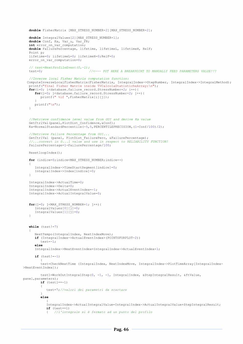
Pag. 46
double FisherMatrix [MAX_STRESS_NUMBER+2][MAX_STRESS_NUMBER+2];
double IntegralValues[2][MAX_STRESS_NUMBER+1];
double Conf, Ka, Var_u, Var_FR;
int error_on_var_computation;
double FailurePercentage, lifetime, lifetimeL, lifetimeH, RelF;
Point p;
lifetime=0; lifetimeL=0; lifetimeH=0;RelF=0;
error_on_var_computation=0;
// test=NextProfileEvent(0,-1);
test=0; //<--- PUT HERE A BREAKPOINT TO MANUALLY FEED PARAMETERS VALUE!!!
//Inverse local Fisher Matrix computation function:
ComputeInverseLocalFisherMatrix(FisherMatrix, IntegralIndex->StepNumber, IntegralIndex->IntegralMethod);
printf("final Fisher Matrix inside TVCalcolaStatisticheArray:\n");
for(i=0; i<database.failure_record.StressNumber+2; i++){
for(j=0; j<database.failure_record.StressNumber+2; j++){
printf(" %lf ",FisherMatrix[i][j]);
}
printf("\n");
}
//Retrieve confidence level value from GUI and derive Ka value
GetCtrlVal(panel,PlotDist_Confidence,&Conf);
Ka=NormalStandardPercentile(-5,5,PERCENTILEPRECISION,(1-Conf/100)/2);
//Retrieve Failure Percentage from GUI...
GetCtrlVal (panel, PlotDist_FailurePerc, &FailurePercentage);
//...convert in 0...1 value and use in respect to RELIABILITY FUNCTION!
FailurePercentage=1-FailurePercentage/100;
ResetloopIndex();
for (indice=0;indice<MAX_STRESS_NUMBER;indice++)
{
IntegralIndex->TimeStartSegment[indice]=0;
IntegralIndex->Index[indice]=0;
}
IntegralIndex->ActualTime=0;
IntegralIndex->Delta=0;
IntegralIndex->ActualEventIndex=-1;
IntegralIndex->ActualIntegralValue=0;
for(j=0; j<MAX_STRESS_NUMBER+1; j++){
IntegralValues[0][j]=0;
IntegralValues[1][j]=0;
}
while (test!=7)
{
NextTempo(IntegralIndex, NextIndexMove);
if (IntegralIndex->ActualEventIndex>(POINTSFORPLOT-2))
test=-1;
else
IntegralIndex->NextEventIndex=IntegralIndex->ActualEventIndex+1;
if (test!=-1)
{
test=CheckNextTime (IntegralIndex, NextIndexMove, IntegralIndex->PlotTimeArray[IntegralIndex-
>NextEventIndex]);
test1=WorkOutIntegralStep(0, -1, -1, IntegralIndex, &StepIntegralResult, &ftValue,
panel,parameters);
if (test1==-1)
{
test=7;//valori dei parametri da scartare
}
else
{
IntegralIndex->ActualIntegralValue=IntegralIndex->ActualIntegralValue+StepIntegralResult;
if (test==1)
{ //l'integrale si è fermato ad un punto del profilo

Pag. 47
//R(t):
IntegralIndex->PlotFRArray[IntegralIndex->ActualEventIndex]=exp(-pow((IntegralIndex-
>ActualIntegralValue),parameters[database.failure_record.StressNumber+1]));
//f(t):
IntegralIndex->PlotFDArray[IntegralIndex->ActualEventIndex]=IntegralIndex-
>PlotFRArray[IntegralIndex->ActualEventIndex]*pow((IntegralIndex-
>ActualIntegralValue),(parameters[database.failure_record.StressNumber+1]-
1))*parameters[database.failure_record.StressNumber+1]/(exp(ftValue));
//FR(t):
IntegralIndex->PlotFIArray[IntegralIndex->ActualEventIndex]=(IntegralIndex-
>PlotFDArray[IntegralIndex->ActualEventIndex])/(IntegralIndex->PlotFRArray[IntegralIndex-
>ActualEventIndex]);
IntegralIndex->PlotFItArray[IntegralIndex->ActualEventIndex]=IntegralIndex-
>ActualIntegralValue;
IntegralIndex->PlotFftArray[IntegralIndex->ActualEventIndex]=ftValue;
//F(t)
IntegralIndex->PlotFCArray[IntegralIndex->ActualEventIndex]=1-IntegralIndex-
>PlotFRArray[IntegralIndex->ActualEventIndex];
test2 = ComputeVarianceReliabilityAndFailureRate(&Var_u, &Var_FR, IntegralIndex,
IntegralValues, FisherMatrix, exp(ftValue), parameters, panel);
if(test2==-1)
MessagePopup("Statistical Analysis Panel Error","Error in the confidence bounds
computation!\nTry to change convergence parameters");
//If the Variance of u function is negative, something is wrong. The cause is the value of
elements of Fisher matrix, which
//depends on the parameters' values computed with the genetic algorithm. The user should,
in this case, execute again the
//genetic algorithm to obtain new values for the parameters!
if((Var_u<0||Var_FR<0) && error_on_var_computation==0){
//test=7;
//If you choose to put test=7, the output will break with succes due to error, but
remember that
//some elements inside arrays will remain not defined => random values from RAM =>
everything can appear on screen
error_on_var_computation=1;
if(Var_u<0 && Var_FR<0){
MessagePopup("Statistical Analysis Panel Error","Due to numeric approximation, for
some points of the plot happens Var(Reliabiity function)<0 and Var(Failure Rate function)<0.\n Confidence
bounds for a few discrete plot points may thus result incorrect.\nYou might try to execute again the
Genetic Algorithm.");
}else{
if(Var_u<0)
MessagePopup("Statistical Analysis Panel Error","Due to numeric approximation, for
some points of the plot happens Var(Reliabiity function)<0.\n Confidence bounds for a few discrete plot
points may thus result incorrect.\nYou might try to execute again the Genetic Algorithm.");
if(Var_FR<0)
MessagePopup("Statistical Analysis Panel Error","Due to numeric approximation, for
some points of the plot happens Var(Failure Rate function)<0.\n Confidence bounds for a few discrete plot
points may thus result incorrect.\nYou might try to execute again the Genetic Algorithm.");
}
}
if(Var_u<0){
printf("TimeElement=%d,TimeArray=%lf->Var=%lf - ",IntegralIndex-
>ActualEventIndex,IntegralIndex->PlotTimeArray[IntegralIndex->ActualEventIndex],Var_u);
}
IntegralIndex->PlotFRArrayLOW[IntegralIndex->ActualEventIndex]=pow(e,-
pow(e,log(pow(IntegralIndex->ActualIntegralValue,parameters[database.failure_record.StressNumber+1]))-Ka*
pow(Var_u,0.5)));
IntegralIndex->PlotFRArrayUP[IntegralIndex->ActualEventIndex]=pow(e,-
pow(e,log(pow(IntegralIndex-
>ActualIntegralValue,parameters[database.failure_record.StressNumber+1]))+Ka*pow(Var_u,0.5)));
IntegralIndex->PlotFCArrayLOW[IntegralIndex->ActualEventIndex]=1-IntegralIndex-
>PlotFRArrayLOW[IntegralIndex->ActualEventIndex];
IntegralIndex->PlotFCArrayUP [IntegralIndex->ActualEventIndex]=1-IntegralIndex-
>PlotFRArrayUP[IntegralIndex->ActualEventIndex];
IntegralIndex->PlotFIArrayLOW[IntegralIndex->ActualEventIndex]=IntegralIndex-
>PlotFIArray[IntegralIndex->ActualEventIndex]-Ka*pow(Var_FR,0.5);
IntegralIndex->PlotFIArrayUP [IntegralIndex->ActualEventIndex]=IntegralIndex-
>PlotFIArray[IntegralIndex->ActualEventIndex]+Ka*pow(Var_FR,0.5);

Pag. 48
//Due to numerical approximations, some PlotFIArrayLOW (lower boundary of Failure Rate
function) might
//be less than zero. Thus a control is needed: if this situation happens, then we force the
value to be zero.
if(IntegralIndex->PlotFIArrayLOW[IntegralIndex->ActualEventIndex]<0){
IntegralIndex->PlotFIArrayLOW[IntegralIndex->ActualEventIndex]=0;
}
//LIFETIME value check
if(IntegralIndex->PlotFRArray[IntegralIndex->ActualEventIndex]>FailurePercentage){
lifetime=IntegralIndex->PlotTimeArray[IntegralIndex->ActualEventIndex];
RelF=IntegralIndex->PlotFRArray[IntegralIndex->ActualEventIndex];
}
if(IntegralIndex->PlotFRArrayLOW[IntegralIndex->ActualEventIndex]>FailurePercentage){
lifetimeL=IntegralIndex->PlotTimeArray[IntegralIndex->ActualEventIndex];
}
if(IntegralIndex->PlotFRArrayUP[IntegralIndex->ActualEventIndex]>FailurePercentage){
lifetimeH=IntegralIndex->PlotTimeArray[IntegralIndex->ActualEventIndex];
}
}
GoToNextTime(IntegralIndex, NextIndexMove);
}
}
else
{ //-1=punti del profilo finiti
test=7;
}
}
if (test1==-1)
return -1;
else
//Write on GUI Lifetime, LifetimeH and LifetimeL values
SetCtrlVal (panel, PlotDist_LifeTime, lifetime);
if(lifetimeL!=0){
SetCtrlVal (panel, PlotDist_LifeTimeL, lifetimeH);
}else{
SetCtrlAttribute (panel, PlotDist_LifeTimeL, ATTR_TEXT_COLOR, VAL_GRAY);
}
if(lifetimeH!=0){
SetCtrlVal (panel, PlotDist_LifeTimeH, lifetimeL);
}else{
SetCtrlAttribute (panel, PlotDist_LifeTimeH, ATTR_TEXT_COLOR, VAL_GRAY);
}
//Write on GUI the Shape parameter beta
SetCtrlVal (panel, PlotDist_scale,
database.ParameterEstimation.GLLWeibullParam[database.failure_record.StressNumber+1]);
//Write on GUI the Reliabilty value
SetCtrlVal (panel, PlotDist_RelF, RelF);
//Set other elements as GREY '0.0000' because not computable:
SetCtrlAttribute (panel, PlotDist_shapeInf, ATTR_TEXT_COLOR, VAL_GRAY);
SetCtrlAttribute (panel, PlotDist_shapeSup, ATTR_TEXT_COLOR, VAL_GRAY);
SetCtrlAttribute (panel, PlotDist_RelFL, ATTR_TEXT_COLOR, VAL_GRAY);
SetCtrlAttribute (panel, PlotDist_RelFH, ATTR_TEXT_COLOR, VAL_GRAY);
SetCtrlAttribute (panel, PlotDist_scaleSup, ATTR_TEXT_COLOR, VAL_GRAY);
SetCtrlAttribute (panel, PlotDist_shape, ATTR_TEXT_COLOR, VAL_GRAY);
SetCtrlAttribute (panel, PlotDist_scaleInf, ATTR_TEXT_COLOR, VAL_GRAY);
SetCtrlAttribute (panel, PlotDist_MTBF, ATTR_TEXT_COLOR, VAL_GRAY);
return 0;
}
11.5 WorkOutIntegralStep function source code
int WorkOutIntegralStep(int integraltype, int i, int j, struct IntegralIndex * IntegralIndex,double *
StepIntegralResult, double * ftValue, int panel, double * parameters)
{
double Delta;
double ArrayTime [50];
double ArrayValue [50];
double NextStep;
double ft;
int indice, indice1;
int StepNumber;
int IntegralMethod;

Pag. 49
int test,test1,r,s,stress, stress_index;
double Stress1, Delta1, Stress2, Delta2;
//GetCtrlVal(panel,AGcalc_AGIntStepPoints,&StepNumber);
//GetCtrlVal(panel,AGcalc_AGSelMet,&IntegralMethod);
Delta=IntegralIndex->Delta/(IntegralIndex->StepNumber-1);
NextStep=0;
for (indice1=0;indice1<IntegralIndex->StepNumber;indice1++)
{
ArrayTime[indice1]=IntegralIndex->ActualTime+NextStep;
test1=WorkOutft(IntegralIndex, ArrayTime[indice1], &ft,parameters);
if ((-ft)<700)
{
switch(integraltype){
case 0: ArrayValue[indice1]=exp(-ft);
break;//ft
case 11: r=(i-1)-1;
if(r>=0){
//it is a real stress, let us find which one!
stress=-1;
for(stress_index=0; stress_index<MAX_STRESS_NUMBER; stress_index++){
if(database.failure_record.stress[stress_index]==1){
stress=stress+1;
}
if(stress==r){
//stress is the index of stress to be considered (pointed into stress vector)
Stress1=(ArrayTime[indice1]-IntegralIndex-
>TimeStartSegment[stress_index])*database.TVProfileTableArray[IntegralIndex-
>Profilo].TVProfile[stress_index].Value[2][IntegralIndex-
>Index[stress_index]]+database.TVProfileTableArray[IntegralIndex-
>Profilo].TVProfile[stress_index].Value[1][IntegralIndex->Index[stress_index]];
Delta1=X_switch(Stress1, stress_index);
//interrupt loop execution!
stress_index=MAX_STRESS_NUMBER;
}
}
}else{
Delta1=1;
}
ArrayValue[indice1]=Delta1*exp(-ft);
break;
case 12: s=(j-1)-1;
if(s>=0){
//it is a real stress, let us find which one!
stress=-1;
for(stress_index=0; stress_index<MAX_STRESS_NUMBER; stress_index++){
if(database.failure_record.stress[stress_index]==1){
stress=stress+1;
}
if(stress==s){
//stress is the index of stress to be considered (pointed into stress vector)
Stress1=(ArrayTime[indice1]-IntegralIndex-
>TimeStartSegment[stress_index])*database.TVProfileTableArray[IntegralIndex-
>Profilo].TVProfile[stress_index].Value[2][IntegralIndex-
>Index[stress_index]]+database.TVProfileTableArray[IntegralIndex-
>Profilo].TVProfile[stress_index].Value[1][IntegralIndex->Index[stress_index]];
Delta1=X_switch(Stress1, stress_index);
//interrupt loop execution!
stress_index=MAX_STRESS_NUMBER;
}
}
}else{
Delta1=1;
}
ArrayValue[indice1]=Delta1*exp(-ft);
/* when WorkOutIntegralStep is called by ComputeVarianceReliabilityAndFailureRate, it is
necessary to return Delta1 value as well! It is required into this higher-level
function in order to perform further needed computations...
The "return" uses *ftValue that is not used in WorkOutIntegralStep CASE 12.
*/
break;
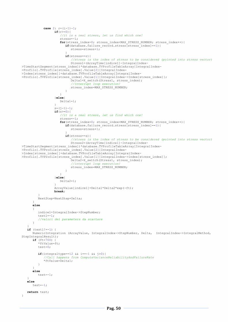
Pag. 50
case 2: r=(i-1)-1;
if(r>=0){
//it is a real stress, let us find which one!
stress=-1;
for(stress_index=0; stress_index<MAX_STRESS_NUMBER; stress_index++){
if(database.failure_record.stress[stress_index]==1){
stress=stress+1;
}
if(stress==r){
//stress is the index of stress to be considered (pointed into stress vector)
Stress1=(ArrayTime[indice1]-IntegralIndex-
>TimeStartSegment[stress_index])*database.TVProfileTableArray[IntegralIndex-
>Profilo].TVProfile[stress_index].Value[2][IntegralIndex-
>Index[stress_index]]+database.TVProfileTableArray[IntegralIndex-
>Profilo].TVProfile[stress_index].Value[1][IntegralIndex->Index[stress_index]];
Delta1=X_switch(Stress1, stress_index);
//interrupt loop execution!
stress_index=MAX_STRESS_NUMBER;
}
}
}else{
Delta1=1;
}
s=(j-1)-1;
if(s>=0){
//it is a real stress, let us find which one!
stress=-1;
for(stress_index=0; stress_index<MAX_STRESS_NUMBER; stress_index++){
if(database.failure_record.stress[stress_index]==1){
stress=stress+1;
}
if(stress==s){
//stress is the index of stress to be considered (pointed into stress vector)
Stress2=(ArrayTime[indice1]-IntegralIndex-
>TimeStartSegment[stress_index])*database.TVProfileTableArray[IntegralIndex-
>Profilo].TVProfile[stress_index].Value[2][IntegralIndex-
>Index[stress_index]]+database.TVProfileTableArray[IntegralIndex-
>Profilo].TVProfile[stress_index].Value[1][IntegralIndex->Index[stress_index]];
Delta2=X_switch(Stress1, stress_index);
//interrupt loop execution!
stress_index=MAX_STRESS_NUMBER;
}
}
}else{
Delta2=1;
}
ArrayValue[indice1]=Delta1*Delta2*exp(-ft);
break;
}
NextStep=NextStep+Delta;
}
else
{
indice1=IntegralIndex->StepNumber;
test1=-1;
//valori dei parameters da scartare
}
}
if (test1!=-1) {
NumericIntegration (ArrayValue, IntegralIndex->StepNumber, Delta, IntegralIndex->IntegralMethod,
StepIntegralResult);
if (ft<700) {
*ftValue=ft;
test=0;
if(integraltype==12 && i==-1 && j>0){
//Call happens from ComputeVarianceReliabilityAndFailureRate
*ftValue=Delta1;
}
}
else
test=-1;
}
else
test=-1;
return test;
}

Pag. 51
12 APPENDIX B - Derivation steps of each term of Fisher Matrix
The goal of this Appendix is to show the passages to perform in order to compute each element of
the Fisher matrix. We will see that the derivation of MLE function introduces some simplifications to
take into account in order to obtain a compact expression of it.
Regarding derivation, some mathematical proprieties need to be applied:
Swapping of the operators of derivation and sum;
Swapping of the operators of derivation and integration. We assume this is always possible
in our analysis because we deal with integrand functions that meets the hypothesis of some
theorems: the integration domain is a subdomain of R; all hypothesis of theorem of passage
to the limit under the classic derivative hold; the integrand function is limited inside the
integration interval;
Derivation of product functions and exponential ones, also remembering the sign of the
exponential when moved from denominator to numerator of a fraction (and vice versa).
We start with the recall of function in the form of Equation 5.2-1 , taking into account Equation 4.5-1
and in the form of Equation 4.3-3.
12.1 Computation of
We start by applying the derivative operator to the function:
∑{ [
] }
∑
Equation
12.1-1
The operators of derivation and sum are thus swapped:
∑
{ [
] }
∑
Equation
12.1-2
It is now sufficient to compute the first order derivative of a logarithmic function and of an
exponential one. The term , when derived in respect to , must be thought in the form of ,
with real number and the variable in respect to which we perform the derivation operation:
∑{
}
∑
Equation
12.1-3
The common terms are thus collected together, in order to obtain a more compact form of the
expression:
∑{
}
∑
Equation
12.1-4
We finally lead to the result:

Pag. 52
∑{
}
∑
Equation
12.1-5
12.2 Computation of
The derivation of the MLE-log function in respect, again, to the same variable is just a matter of
reconsidering the previously derived expression ( Equation 12.1-5 ) and applying again the same rules
of derivation:
(
) ∑{
(
)
}
∑
Equation
12.2-1
The final result comes immediately:
∑{
}
∑
Equation
12.2-2
From now on, we will start to derive the MLE function in respect to coefficients. In order to
generalize those derivatives and not to distinguish between and , we can write:
∑ ∑
|
Equation
12.2-3
12.3 Computation of
The derivative operator is applied to the MLE function. This time, we should not forget that the
derivation is done in respect to the generic parameter. It appears more times than in the
expression of , thus a longer and a slightly more complex derivation process will result:
∑{ [
] }
∑
Equation
12.3-1
For a better readability of the sequence of the operations, it appears appropriate to split the first
sum in two terms:
∑ [
]
∑
∑
Equation
12.3-2
After splitting the algebraic sum, the derivation process can start and, for each term, the derivative
operator can be swapped with the sum one:

Pag. 53
∑
[
]
∑
∑
Equation
12.3-3
At least at the beginning of the derivation process, we deal with similar operations already
performed in Equation 12.1-3. However, this time the variable in respect to which to derivate is also
present inside the function , thus the derivation of the logarithm must be a careful task:
∑
[
]
∑
∑
Equation
12.3-4
Start writing the explicit form of terms and is a good idea, to recognize when and how to derive
the argument of the logarithm:
∑ ∑
∫ (
∑
)
[ ∑
∫ (
∑
)
]
∑
∫ (
∑
)
∑
∫ (
∑
)
Equation
12.3-5
It is convenient to split the two exponential terms in two part: the one which is independent on
coefficient, ∑ , and another one which only contains the term: . In
the function of the first sum term to be derived, the independent part ∑ can thus
be moved outside the operator of derivation:
∑ ∑
∫ (
∑
)
∑
[ ∫ (
∑
)
]
∑
∫ (
∑
)
∑
∫ (
∑
)
Equation
12.3-6
The two exponential terms, constant in respect to and with opposite sign, can be simplified. In
the meantime, the derivative of the product of two functions, which are present in the first
summation term, can be carried out:
∑
[ ∫
(
∑
)
]
∑∫
(
∑
)
∑ ∫
(
∑
)
Equation
12.3-7
The terms and can be again simplified, while the last derivative is
performed. This time it regards . The difference in respect to Equation 12.1-3 is that now is

Pag. 54
function of the derivation variable and not anymore a constant. The constant is now . While
performing the derivative, we remember that the derivation and integration operators can be
swapped, thus it is just a matter of deriving
∑
. While applying the usual rules of
derivation, it is convenient to split again the exponential term in the usual two parts and
remembering which of them is constant. The same approach is applied to
∑
term:
∑
[ ∫
∑
(
)
]
∑ ∫
∑
(
)
∑ ∫
∑
(
)
Equation
12.3-8
The final derivations are now performed:
∑
[ ∫
∑
]
∑ ∫
∑
∑ ∫
∑
Equation
12.3-9
Further simplifications can be done in the first sum term, in respect to the exponential terms
and :
∑[ ∫
∑
]
∑ ∫
∑
∑ ∫
∑
Equation
12.3-10
The first two sum terms can be joint back:

Pag. 55
∑[ { } ∫
∑
]
∑ ∫
∑
Equation
12.3-11
The latter operation leads to the final expression of this derivative:
∑[ { ( ) } ∫
∑
]
∑ ∫
∑
Equation
12.3-12
12.4 Computation of
The expression in Equation 12.3-12 can be taken into account in order to perform the second mixed
derivative in respect, now, to :
(
) ∑
[
{ ( ) } ∫
∑
]
∑
( ∫
∑
)
Equation
12.4-1
After applying trivial derivation properties to the terms which depends on parameter, the final
expression can be found:
∑[ { } ∫
∑
]
∑[{ }∫
∑
]
Equation
12.4-2
12.5 Computation of
The final goal of this analytical analysis is to compute the second order partial derivative of the MLE-
log function in respect to two different parameters and , remembering that they both lie in the
range . Starting from the result obtained in Equation 12.3-12, it is possible to derive the function

Pag. 56
in respect to . Let us make things a bit faster now, starting from swapping the operators of
derivation and summation:
(
) ∑
[ { ( ) } ∫
∑
]
∑
( ∫
∑
)
Equation
12.5-1
Before going on, it is convenient again to make explicit the integral function , like in Equation 12.3-5:
∑
[ ∫ (
∑
)
∫
∑
{ (∫ (
∑
)
)}]
∑
( ∫ (
∑
)
∫
∑
)
Equation
12.5-2
Inside the graph parenthesis, is now multiplied by the two inner terms:
∑
[ ∫ (
∑
)
∫
∑
{ ∫ (
∑
)
}]
∑
( ∫ (
∑
)
∫
∑
)
Equation
12.5-3
Further work can be done on the graph parenthesis, by multiplying its content by the two integral
functions. Consider this work as preparative for the application of derivation in respect to :
∑
[∫ (
∑
)
∫
∑
∫ (
∑
)
∫
∑
∫ (
∑
)
∫
∑
]
∑
( ∫ (
∑
)
∫
∑
)
Equation
12.5-4
The common terms are collected and the sums are split into three terms for a better management
during the derivation process that will follow:
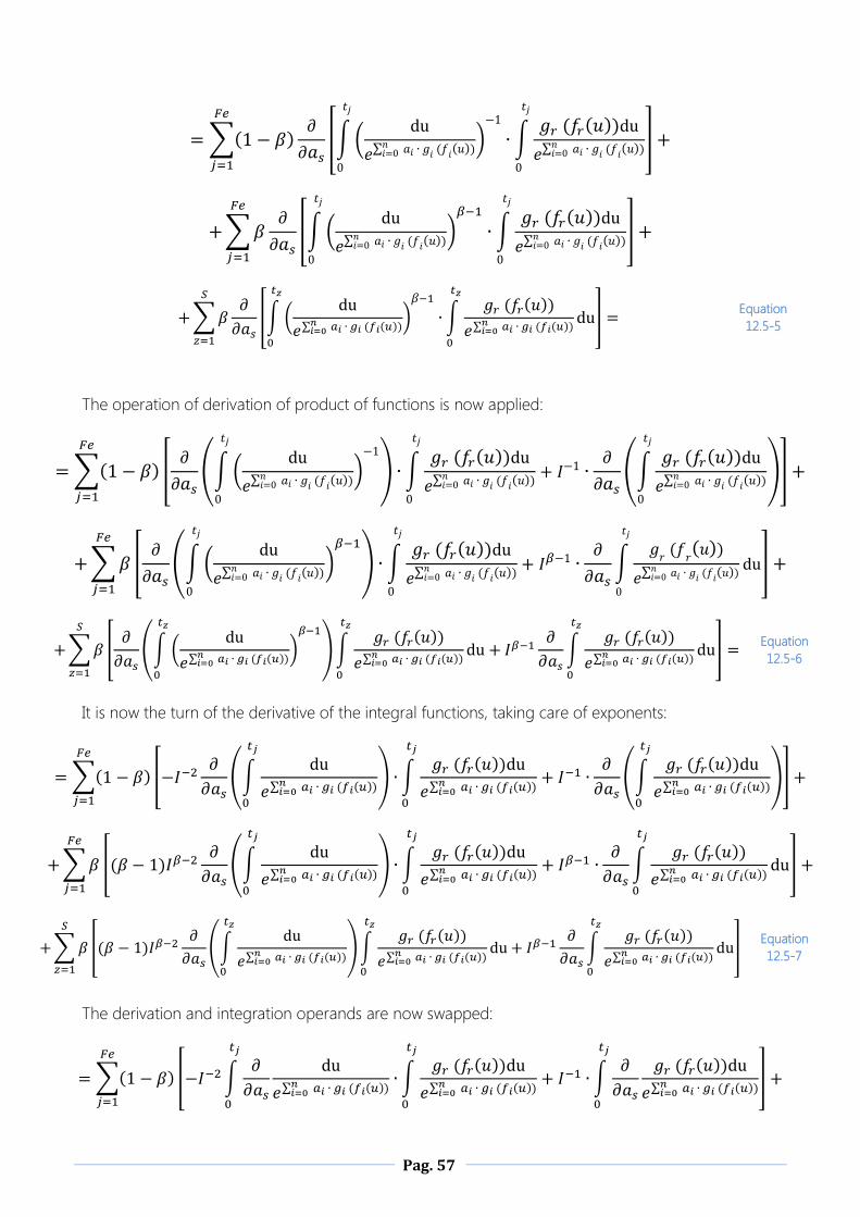
Pag. 57
∑
[∫ (
∑
)
∫
∑
]
∑
[∫ (
∑
)
∫
∑
]
∑
[∫ (
∑
)
∫
∑
]
Equation
12.5-5
The operation of derivation of product of functions is now applied:
∑ [
(∫ (
∑
)
) ∫
∑
(∫
∑
)]
∑ [
(∫ (
∑
)
) ∫
∑
∫
∑
]
∑ [
(∫ (
∑
)
)∫
∑
∫
∑
]
Equation
12.5-6
It is now the turn of the derivative of the integral functions, taking care of exponents:
∑ [
(∫
∑
) ∫
∑
(∫
∑
)]
∑ [
(∫
∑
) ∫
∑
∫
∑
]
∑ [
(∫
∑
)∫
∑
∫
∑
]
Equation
12.5-7
The derivation and integration operands are now swapped:
∑ [ ∫
∑
∫
∑
∫
∑
]
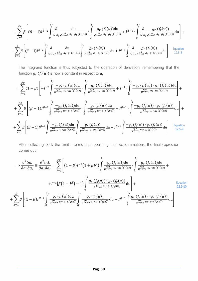
Pag. 58
∑ [ ∫
∑
∫
∑
∫
∑
]
∑ [ ∫
∑
∫
∑
∫
∑
]
Equation
12.5-8
The integrand function is thus subjected to the operation of derivation, remembering that the
function is now a constant in respect to :
∑ [ ∫
∑
∫
∑
∫
∑
]
∑ [ ∫
∑
∫
∑
∫
∑
]
∑ [ ∫
∑
∫
∑
∫
∑
]
Equation
12.5-9
After collecting back the similar terms and rebuilding the two summations, the final expression
comes out:
∑[ ( )∫
∑
∫
∑
{ ( ) }∫
∑
]
∑ [ ∫
∑
∫
∑
∫
∑
]
Equation
12.5-10

Pag. 59
13 APPENDIX C – Computation steps of Reliability function derivatives
The same general derivation rules already seen in the previous Appendix applies to both for the
Reliability function derivatives and the Failure Rate function derivatives.
13.1 Derivative in respect to parameter
This derivative is quite trivial to get since the integral function does not depend on :
Equation
13.1-1
Equation
13.1-2
13.2 Derivative in respect to each parameters
The integral function depends instead on each parameter , with , thus it is convenient
to write into its explicit form:
[(∫
∑
)
] Equation
13.2-1
First of all, the derivative of the logarithm must be computed:
(∫
∑
) Equation
13.2-2
Then, we proceed to compute the derivative of the logarithm’s argument (that is, the integral
function); the derivation operator can be moved as usual inside the integral:
∫
∑
Equation
13.2-3
The integrand function can be split in two parts: the one that depends on parameter and the
one that is constant in respect to it:
∫
∑
Equation
13.2-4
Finally the inner derivative of the fraction with the exponential can be performed:
∫
∑
Equation
13.2-5
Final simplifications lead to the final expression:
∫
∑
Equation
13.2-6

Pag. 60
14 APPENDIX D - Computation steps of Failure Rate function derivatives
The form of the Failure Rate derivatives are a little more complex than the ones of the derived
in the previous Appendix. Each parameter appears more than once; derivatives of products and
ratios must be performed.
14.1 Derivative in respect to parameter
The Equation 7.4-2 represents the form of the Failure Rate function and thus it is the starting point for
the computation of each derivative. Once again, since the integral function does not depend on ,
it is convenient to keep into its implicit form:
(
∑
) Equation
14.1-1
The term ∑ is constant in respect to and can be moved outside the derivation
operator:
∑
( )
Equation
14.1-2
The derivative to compute is now a simple derivative of the product of two functions:
∑
[ ] Equation
14.1-3
The final expression is:
∑
Equation
14.1-4
14.2 Derivative in respect to each parameters
Inside the expression of the Failure Rate function there is an heavy presence of the parameters ,
with . This implies to handle with the most explicit possible form of the function while
derivation operations are performed.
[
∑
(∫
∑
)
] Equation
14.2-1
We start with the derivative of the product among two functions:
{
[
∑
]
∑
[(∫
∑
)
]}
Equation
14.2-2

Pag. 61
Focusing on the first derivative, it is, as usual, convenient to split the exponential sum term for the
first derivative; in the meanwhile the first (“outer”) part of the second derivative can be performed:
{
(
∑
)
∑
(∫
∑
)}
Equation
14.2-3
While completing the calculus of the first derivative, regarding the second derivative we can move
the derivation operator inside the integral close to the integrand function:
{
∑
∑
∫
∑
}
Equation
14.2-4
The same “split” operation can be applied again to the integrand function:
{
∑
∑
∫
∑
}
Equation
14.2-5
The last derivative can be performed to obtain the final result:
{
∑
∑
∫
∑
}
Equation
14.2-6
The final expression is:
∑
{ ∫
∑
} Equation
14.2-7

Pag. 62
15 References
www.Weibull.com website
“Life Data Analysis Reference” - ReliaSoft Publishing, Rev. 2005
“Accelerated Life Testing Reference” - ReliaSoft Publishing, Rev. 2007
“Accelerated Testing statistical model, test plans and Data Analyses” - Wayne Nelson,
published by John Wiley & Sons Inc. 1990
“Applied life Data Analysis” - Wayne Nelson, published by John Wiley & Sons Inc. 1982
"Reliability Confidence Limits with the Weibull Distribution" - Copyright © 1999 by
Engineered Software, Inc.
"Analisi affidabilistica delle centraline elettroniche per il controllo di motori per trazione civile",
section “Intervalli di confidenza”, subsections from 4.1 to 4.3 - Master degree Thesis at
Politecnico di Torino
"Progettazione e realizzazione del sistema elettronico di controllo per le batterie di trazione
nei veicoli ibridi", section "Analisi affidabilistica dei componenti elettronici", Master Degree
Thesis of Marco Elia at Politecnico di Torino.